| Issue |
A&A
Volume 653, September 2021
|
|
|---|---|---|
| Article Number | A19 | |
| Number of page(s) | 17 | |
| Section | Cosmology (including clusters of galaxies) | |
| DOI | https://doi.org/10.1051/0004-6361/202140795 | |
| Published online | 02 September 2021 | |
AMICO galaxy clusters in KiDS-DR3
Cosmological constraints from large-scale stacked weak lensing profiles
1
INAF – Osservatorio di Astrofisica e Scienza dello Spazio di Bologna, Via Gobetti 93/3, 40129 Bologna, Italy
e-mail: carlo.giocoli@inaf.it
2
Dipartimento di Fisica e Astronomia “Augusto Righi”, Alma Mater Studiorum Università di Bologna, Via Gobetti 93/2, 40129 Bologna, Italy
3
INFN – Sezione di Bologna, Viale Berti Pichat 6/2, 40127 Bologna, Italy
4
Dipartimento di Fisica, Università degli Studi Roma Tre, Via della Vasca Navale 84, 00146 Rome, Italy
5
INFN – Sezione di Roma Tre, Via della Vasca Navale 84, 00146 Rome, Italy
6
Zentrum für Astronomie, Universität Heidelberg, Philosophenweg 12, 69120 Heidelberg, Germany
7
ITP, Universität Heidelberg, Philosophenweg 16, 69120 Heidelberg, Germany
8
INAF – Osservatorio Astronomico di Padova, Vicolo dell’Osservatorio 5, 35122 Padova, Italy
9
Dipartimento di Fisica “E. Pancini”, Universitá di Napoli Federico II, C.U. di Monte Sant’Angelo, Via Cintia, 80126 Napoli, Italy
10
INAF – Osservatorio Astronomico di Capodimonte, Salita Moiariello 16, 80131 Napoli, Italy
11
INFN – Sezione di Napoli, Via Cintia, 80126 Napoli, Italy
12
Astrophysics Research Institute, Liverpool John Moores University, 146 Brownlow Hill, Liverpool L3 5RF, UK
13
School of Mathematics, Statistics and Physics, Newcastle University, Herschel Building, NE1 7RU Newcastle-upon-Tyne, UK
14
Institute of Cosmology & Gravitation, University of Portsmouth, Dennis Sciama Building, Portsmouth PO1 3FX, UK
Received:
12
March
2021
Accepted:
27
May
2021
Context. The large-scale mass distribution around dark matter haloes hosting galaxy clusters provides sensitive cosmological information.
Aims. In this work we make use of a large photometric galaxy cluster sample, constructed from the public Third Data Release of the Kilo-Degree Survey, and the corresponding shear signal, to assess cluster masses and test the concordance Λ-cold dark matter (ΛCDM) model. In particular, we study the weak gravitational lensing effects on scales beyond the cluster virial radius, where the signal is dominated by correlated and uncorrelated matter density distributions along the line of sight. The analysed catalogue consists of 6962 galaxy clusters, in the redshift range 0.1 ≤ z ≤ 0.6 and with signal-to-noise ratios higher than 3.5.
Methods. We perform a full Bayesian analysis to model the stacked shear profiles of these clusters. The adopted likelihood function considers both the small-scale one-halo term, used primarily to constrain the cluster structural properties, and the two-halo term, that can be used to constrain cosmological parameters.
Results. We find that the adopted modelling is successful in assessing both the cluster masses and the total matter density parameter, ΩM, when fitting shear profiles up to the largest available scales of 35 Mpc h−1. Moreover, our results provide a strong observational evidence of the two-halo signal in the stacked gravitational lensing of galaxy clusters, further demonstrating the reliability of this probe for cosmological studies. The main result of this work is a robust constraint on ΩM, assuming a flat ΛCDM cosmology. We get ΩM = 0.29 ± 0.02, estimated from the full posterior probability distribution, consistent with the estimates from cosmic microwave background experiments.
Key words: cosmological parameters / large-scale structure of Universe / gravitational lensing: weak / surveys / dark matter / galaxies: clusters: general
© ESO 2021
1. Introduction
The standard Λ-cold dark matter (ΛCDM) cosmological model provides the most convenient and simplest parametrisation of the Concordance Model. Recent wide-field observational surveys have provided stringent constraints on the two most significant energy-density constituents of our Universe: dark energy and dark matter. While the first contributes to about ∼68% of the total mass-energy, the second constitutes about ∼27% (Bennett et al. 2013; Planck Collaboration I 2014; Planck Collaboration XIII 2016; Planck Collaboration VI 2020). The current consensus is that this dark matter component is mainly cold, being composed of particles moving at non-relativistic speeds. Only ∼5% of the Universe is made up of ordinary matter (baryons), and even less is made up of radiation (∼10−5).
The ΛCDM model is not based on any particular assumption about the nature and physical origin of the dark components. Nevertheless, it is currently the best cosmological model available to describe the large-scale structure of the Universe and its evolution. Moreover, different observations (Hikage et al. 2019; Hamana et al. 2020; Bautista et al. 2021) show that the geometry of our Universe is flat on large scales, so that the Concordance Model is often also called the flat ΛCDM model.
In this scenario clusters of galaxies play an important role both in constraining cosmological parameters (Sheth & Tormen 1999; Tormen 1998; Borgani & Kravtsov 2011) and in the study of the formation and evolution of the galaxies in their environment (Springel et al. 2001; Borgani et al. 2004; Andreon 2010; Angulo et al. 2012; Zhang et al. 2016; Zenteno et al. 2016). Galaxy clusters are hosted by the most massive virialised CDM haloes, and their redshift evolution (number density and spatial distribution) is highly sensitive to different cosmological parameters (see e.g. Planck Collaboration XXIV 2016; Vikhlinin et al. 2009; Veropalumbo et al. 2014, 2016; Sereno et al. 2015; Pacaud et al. 2018; Marulli et al. 2018, 2020; Costanzi et al. 2019; Moresco et al. 2020; Lesci et al. 2020; Nanni et al., in prep.).
By exploiting the optical and near-infrared bands it is possible to identify clusters by searching for the cluster-scale overdensities in the 3D galaxy distribution of wide field observations. This technique allows us to cover large and deep areas of the sky through photometric surveys, providing the possibility to collect a sufficiently large number of clusters and use them as a cosmological tool. Ongoing and planned photometric surveys will allow us to increase the present census of galaxy clusters by orders of magnitude, expanding their detection towards lower masses and higher redshifts (LSST Science Collaboration 2009; Laureijs et al. 2011; Spergel et al. 2013; Sartoris et al. 2016).
However, in order to use galaxy clusters as probes to infer cosmological parameters it is crucial to derive precise and reliable cluster mass estimates (Meneghetti et al. 2010; Giocoli et al. 2014). In particular, the measured number of galaxy cluster members, accessible in photometric or spectroscopic observations, are typically used as mass-proxy, to be linked to the total mass of the cluster (Simet et al. 2017; Murata et al. 2019). Calibrating the relationship between mass-proxy and the true 3D mass is often challenging, and is sometimes hidden in complex and not yet well understood astrophysical processes (Rasia et al. 2012, 2013; Angelinelli et al. 2020).
The most reliable approach for estimating cluster masses is currently provided by the gravitational lensing signal on background galaxies (Bartelmann & Schneider 2001; Umetsu 2020). The robustness of this method relies on the fact that it does not require any assumption on the dynamical state of the luminous and dark matter, being sensitive only to the total projected matter density distribution between the sources and the observer. In particular, the weak lensing effect consists of slight distortions of the source shapes (called shear) and the intensification of their apparent brightness (magnification) caused by the deflection and the convergence of light rays travelling from the sources to the observer. The weak lensing comes into play when the source is at large angular distances from the geometric centre of the lens. Hence it is also very useful to probe the lensing cluster profiles up to large radii. All of these properties made the weak lensing extremely powerful to probe the mass density distributions in clusters on different scales (Sereno et al. 2018).
A small number of background galaxies limits the study of individual cluster masses down to few times 1014 M⊙ for typical current optical surveys. In order to reach a high signal-to-noise ratio (S/N) in the weak lensing mass estimate it is a common practice to stack the weak lensing signals of systems in the same redshift and observable bins by averaging the number of slightly distorted galaxy images in radial bins to increase the shear estimate and reduce the noise; the resultant signal is that of the mass-weighted ensemble. Specifically, the stacked gravitational lensing represents the cross-correlation between foreground deflector positions and background galaxy shears. Given a shallow but broad survey, stacking the signal around a large number of lenses is an efficient way to compensate for the low number density of lensed sources. For example, this approach was applied with great success to the Sloan Digital Sky Survey (SDSS) data to measure the ensemble averaged lensing signal around groups and clusters (Mandelbaum et al. 2006; Sheldon et al. 2009). By splitting the sample of clusters into subsets based on an observable property, such as amplitude or optical richness, it is possible to determine the scaling relations between the observable and the mean mass of the sample (see e.g. Bellagamba et al. 2019).
In this work we exploit the dataset from the Kilo Degree Survey (KiDS; de Jong et al. 2013). The principal scientific goal of KiDS is to exploit the weak lensing and photometric redshift measurements to map the large-scale distribution of matter in the Universe.
Appropriate algorithms have to be used to identify galaxy clusters in photometric surveys. In this work we exploit the Adaptive Matched Identifier of Clustered Objects (AMICO) algorithm, presented and tested in Bellagamba et al. (2018), and used to extract the cluster sample from KiDS-DR3 by Maturi et al. (2019). AMICO is an algorithm for the detection of galaxy clusters in photometric surveys where the dataset is affected by a noisy background. It is built upon a linear optimal matched filter method (Maturi et al. 2005, 2007; Viola et al. 2010; Bellagamba et al. 2011), which maximises the S/N taking advantage of the statistical properties of the field and cluster galaxies.
We build the shear profile of our lens samples following the conservative approach detailed in Bellagamba et al. (2019), then stack the profile signal to increase the S/N. We determine the weighted ellipticity of the background sources in radial bins, that is the tangential and cross components of the shear. In our subsequent analyses we use only the tangential component, hence effectively measuring the shear-cluster correlation function.
For most of the clusters in the sample the S/N in the shear data is too low to constrain the density profile and, consequently, to measure a reliable mass. Thus, we can only measure the mean mass for ensembles of objects chosen according to their observables and redshift. In short, we exploit the shear-cluster correlation (or stacked lensing). The main goal of this work is to assess both the cluster masses and the total matter density parameter, ΩM, modelling the shear-cluster correlation up to the largest available scales.
The statistical numerical code was built with the CosmoBolognaLib (V5.3), a set of free software C++/Python libraries (Marulli et al. 2016) that provide all the functions used for the estimation of the various cosmological components of our fitting model.
This work is organised as follows. In Sect. 2 we present the observational dataset: shear and cluster catalogues. In Sect. 3 we introduce our theoretical model, used to describe the stacked tangential shear profile of the cluster sample. In Sect. 4 we display our results, then summarise and conclude in Sect. 5.
In all the analyses presented in this work we assume a flat ΛCDM model with baryon density Ωb = 0.0486 and scaled Hubble parameter h = 0.7. The matter density parameter is left free except in the first analysis stage where, to infer reference cluster masses while modelling the one-halo term, it is fixed to ΩM = 0.3. When inferring ΩM from the two-halo modelling, we assume a flat ΛCDM, hence ΩΛ = 1 − ΩM is a derived parameter. The symbol log, if not specified otherwise, refers to the logarithm base 10 of the quantity.
2. Data
KiDS (de Jong et al. 2013) is an optical wide-field imaging survey aiming at mapping 1350 square degrees of extra-galactic sky in two stripes (one equatorial, KiDS-N, and one centred around the South Galactic Pole, KiDS-S) in four broad-band filters (u, g, r, i). The observations are performed with the 268 Megapixels OmegaCAM wide-field imager (Kuijken 2011), owning a mosaic of 32 science CCDs and positioned on the Very Large Telescope (VLT) Survey Telescope (VST). This is an ESO telescope of 2.6 m in diameter, located at the Paranal Observatory (for further technical information about VST see Capaccioli & Schipani 2011). The principal scientific goal of KiDS is to exploit weak lensing and photometric redshift measurements to map the large-scale matter distribution in the Universe. The VST-OmegaCAM is the optimal choice for such a survey, as it was expressly created to give excellent and uniform image quality over a large (1 deg2) field of view with a resolution of 0.21 arcsec pixel−1; a field of view 1 deg wide corresponds to ∼12.5 Mpc h−1 at the median redshift of our lens sample, z ∼ 0.35.
The DR3-KiDS catalogue is composed of about 100 000 sources per square degree, for a total of almost 50 million sources over the full survey area. These data are attentively and uniformly calibrated and made usable in an easily accessible dedicated archive.
We exploit the Third Data Release survey (KiDS-DR3, de Jong et al. 2017), which has been obtained with the same instrumental settings of the other two previous releases (de Jong et al. 2015) that were made public in 2013 (DR1) and 2015 (DR2). KiDS-DR3 extends the total released dataset coverage to approximately 447 deg2 with 440 survey tiles. Therefore, with respect to the other previous releases, it provided a considerable survey area extension. This release also includes photometric redshifts with the corresponding probability distribution functions, a global improved photometric calibration, weak lensing shear catalogues and lensing-optimised image data. Source detection, positions and shape parameters used for weak lensing measurements are all derived from the stacked r-band images, while magnitudes are measured in all filters using forced photometry.
One of the main improvements of KiDS-DR3, compared to DR1 and DR2, is the enhanced photometric calibration and the inclusion of photometric redshift distribution probabilities (see e.g. Kuijken et al. 2015; de Jong et al. 2017). The combined set of the 440 survey tiles of DR3 mostly comprises a small number of large contiguous areas (see Fig. 1). This enables a refinement of the photometric calibration that exploits both the overlap between observations within a filter as well as the stellar colours across filters (de Jong et al. 2017)1.
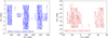 |
Fig. 1. Distribution of cluster centres in angular coordinates of the 6962 detections by AMICO divided into the KiDS-N (left) and KiDS-S (right) areas. Systems with 0.1 ≤ z ≤ 0.6 and with S/N > 3.5 are displayed. |
2.1. Galaxy catalogue
The KiDS galaxy catalogue provides the spatial coordinates, the 2 arcsec aperture photometry in four bands (u, g, r, i) and photometric redshifts for all galaxies down to the 5σ limiting magnitudes of 24.3, 25.1, 24.9, and 23.8, respectively. We chose to avoid the use of galaxy colours to detect clusters in order to minimise the dependence of the selection function on the presence (or absence) of the red-sequence of cluster galaxies (Maturi et al. 2019). For more information about the shear and redshift properties of the entire galaxy catalogue see de Jong et al. (2017) and Hildebrandt et al. (2017).
2.1.1. Galaxy shape measurements
The original shear analysis of the KiDS-DR3 data is described in Kuijken et al. (2015) and Hildebrandt et al. (2017). The shape measurements were performed with lensfit (Miller et al. 2007, 2013) and were successfully calibrated for the KiDS-DR3 data by Fenech Conti et al. (2017).
In this work the data used for shape measurements are those in the r band, being the ones with the best seeing properties and with highest source density. The error on the multiplicative shear calibration, estimated from simulations with lensfit and benefiting from a self-calibration, is of the order of 1% (Hildebrandt et al. 2017). The final catalogue KiDS-DR3 gives shear measurements for ∼15 million galaxies, with an effective number density of neff = 8.53 galaxies arcmin−2 (as defined in Heymans et al. 2012), over a total effective area of 360 deg2.
2.1.2. Galaxy photometric redshifts
The original properties of photometric redshifts (photo-z) of KiDS galaxies are described in Kuijken et al. (2015) and de Jong et al. (2017). The photo-z values were extracted with BPZ (Benítez 2000; Hildebrandt et al. 2012), a Bayesian photo-z estimator based upon template fitting, from the four bands (u, g, r, i). Furthermore, BPZ returns a photo-z posterior probability distribution function which AMICO fully exploits. When compared with spectroscopic redshifts from the Galaxy And Mass Assembly (GAMA, Liske et al. 2015) spectroscopic survey of low redshift galaxies, the resultant accuracy is σz ∼ 0.04(1 + z), as shown in de Jong et al. (2017).
2.2. Cluster catalogue
As already mentioned, the galaxy cluster catalogue we use in this work was extracted from KiDS-DR3 using the AMICO algorithm. In particular, we analysed the same cluster catalogue adopted by Bellagamba et al. (2019). Its full description and validation can be found in Maturi et al. (2019). Here, we present the main properties of this cluster catalogue. It should be noted that the cluster detection through AMICO on KiDS-DR3 is an enhancement of the work by Radovich et al. (2017) on DR2, both in terms of total covered area (438 deg2 against 114 deg2) and of detection algorithm with respect to the previous matched filter method (Bellagamba et al. 2011). From the initial covered 438 deg2, all clusters belonging to those regions heavily affected by satellite tracks, haloes created by bright stars, and image artefacts were rejected (Maturi et al. 2019). Furthermore, we selected only detections with S/N > 3.52. Finally, we narrowed the redshift range to 0.1 ≤ z ≤ 0.6, for a final sample of 6962 galaxy clusters. Objects at z < 0.1 were discarded because of their low lensing power, while those at z > 0.6 were excluded because the background galaxies density in KiDS data is too small to allow a robust weak lensing analysis. Furthermore, collecting clusters with 0.1 ≤ z ≤ 0.6 we can robustly separate the clustered objects from the population of background galaxies. For each cluster we select a galaxy population, excluding the galaxies whose most likely redshift zs is not significantly higher than the lens value zl,
where zs, min is the lower bound of the region including the 2σ of the probability density distribution and Δz is set to 0.05, similar to the typical uncertainty on photometric redshifts in the galaxy catalogue and far larger than the uncertainty on the cluster redshifts.
The criterion based on the photometric redshift distribution aims at keeping only galaxies that have a well-behaved redshift probability distribution and have a negligible probability of being at a redshift equal to or lower than that of the cluster. In addition we consider ≤zs ≤ 1 and the flag ODDS in BPZ to be larger than 0.8: the ODDS parameter indicates the quality of the BPZ photometric redshifts (see Kuijken et al. 2015 for details in the case of KiDS DR3 data).
The left and right panels of Fig. 1 display the angular distribution of galaxy clusters detected by AMICO in the (RA, Dec) coordinate system respectively in the KiDS-N and KiDS-S sky area covered by the DR3 data. We use the masks from the two sky areas to generate random samples of positions, which are needed to construct tangential shear profiles around random points (see the discussion on systematics in Sect. 4).
AMICO searches for cluster candidates by convolving the 3D galaxy distribution with a redshift-dependent filter, defined as the ratio of a cluster signal to a noise model. Such a convolution is able to create a 3D amplitude map, where every peak constitutes a possible detection. Then, for each cluster candidate, AMICO returns angular positions, redshift, S/N, and the signal amplitude A, which is a measure of the cluster galaxy abundance. Bellagamba et al. (2018) demonstrates using simulations that the amplitude is a well-behaved mass-proxy, provided that the model calibration is accurate enough. The signal amplitude is defined as
where θc are the cluster sky coordinates; Mc is the cluster model (i.e. the expected density of galaxies per unit magnitude and solid angle) at the cluster redshift zc; N is the noise distribution; pi(z), θi, and mi indicate the photometric redshift distribution, the sky coordinates and the magnitude of the ith galaxy, respectively; and the parameters α and B are redshift dependent functions providing the normalisation and the background subtraction, respectively.
The cluster model Mc is described by a luminosity function and a radial density profile, obeying the formalism presented in Bellagamba et al. (2018) and derived from the observed galaxy population of clusters detected through the SZ-effect (Hennig et al. 2017), as described in detail in Maturi et al. (2019). Furthermore, AMICO assigns to each galaxy in a sky region a probability to be part of a given detection, defined as
where Aj, θj, and zj are the amplitude, the sky coordinates, and the redshift of the jth detection, respectively, and Pf, i is the field probability of the ith galaxy before the jth detection is defined. In this application to KiDS-DR3 data the adopted filter includes galaxy coordinates, r-band magnitudes, and the full photometric redshift distribution p(z).
The distributions in redshift and amplitude of this sample are shown in Bellagamba et al. (2019). In the following analysis we divide the sample into three redshift bins:
-
0.1 ≤ z < 0.3,
-
0.3 ≤ z < 0.45,
-
0.45 ≤ z ≤ 0.6.
These bins were chosen so that approximately the same number of clusters were included in each bin, and so there were enough clusters to study the amplitude trends.
2.3. Measuring the tangential shear profile
Using the tangential component of the shear signal γt we can write the excess surface mass density as

where Σ(r) represents the mass surface density of the lens at distance r and  its mean within r, and Σcrit indicates the critical surface density (Bartelmann & Schneider 2001) that can be read as
with Dl, Ds, and Dls the angular diameter distances observer-lens, observer-source, and source-lens, respectively; c represents the speed of light and G the universal gravitational constant.
Selecting all background sources of each cluster-lens, as noted above, we can compute the tangential component of the shear with respect to the cluster centre γt. This allows us to construct the excess surface mass density profile at distance rj from the following relation:
Here wi indicates the weight assigned to the measurement of the source ellipticity and K(rj) the average correction due to the multiplicative noise bias in the shear estimate, as in Eq. (7) of Bellagamba et al. (2019). To compute the critical surface density for the ith galaxy we use the most probable source redshift, as given by BPZ.
When stacking the excess surface mass density profile of clusters in equal amplitude and redshift bin we refer to the relation
where N represents the bin in which we perform the stacking and Wn, j indicates the weight for the jth radial bin of the nth cluster:
3. Models
We model the stacked lensing signal with the projected halo model formalism. The total density profile is constructed considering the signal coming from the central part of the cluster, called the one-halo term, and the one caused by correlated large-scale structures, called the two-halo term.
3.1. The one-halo lens model
The radial density profile of the cluster main halo is modelled considering a smoothly truncated Navarro-Frenk-White (NFW; Navarro et al. 1997) density profile (Baltz et al. 2009)
where ρs represents the typical matter density within the scale radius rs; and rt indicates the truncation radius, typically expressed in terms of the halo radius R200, the radius enclosing 200 times the critical density of the Universe at the considered redshift ρc(z): rt = t R200 with t the truncation factor. The scale radius is commonly parametrised as rs = R200/c200, where c200 represents the concentration parameter, which is correlated with the halo mass and redshift depending on the halo mass accretion history (Macciò et al. 2007, 2008; Neto et al. 2007; Zhao et al. 2009; Giocoli et al. 2012a). The total mass enclosed within the radius R200, M200, can be seen as the normalisation of the model and a mass-proxy of the true enclosed mass of the dark matter halo hosting the cluster (Giocoli et al. 2012b).
This truncated version of the NFW model was deeply tested in simulations by Oguri & Hamana (2011), demonstrating that it describes the cluster profiles more accurately than the original NFW profile model, up to about 10 times the radius enclosing 200 times the critical density of the Universe. One of the main advantages of the truncation radius is that it removes the non-physical divergence of the total mass at large radii. Moreover, the Baltz et al. (2009) model describes accurately the transition between the cluster main halo and the two-halo contributions (Cacciato et al. 2009, 2012; Giocoli et al. 2010), providing less biased estimates of mass and concentration from shear profiles (Sereno et al. 2017). Neglecting the truncation the mass would be underestimated and the concentration overestimated. As we are considering only stacked shear profiles, the NFW model provides a reliable description even though it is based on the assumption of spherical symmetry. When stacking several shear profiles the intrinsic halo triaxiality tends to assume a spherical radial symmetry on the stacked profile, for statistical reasons. This is the reason why the weak lensing cross-correlation provides a direct estimate of the mean mass for clusters in a given range of observable properties. As reference model, we set rt = 3 for every amplitude and redshift bin, as was done by Bellagamba et al. (2019), among others, following the results by Oguri & Hamana (2011). However, we discuss how the mass and concentration estimates change when assuming different values of the truncation radius.
When analysing the weak lensing by clusters, an important source of bias is the inaccurate identification of the lens centre. In this study we assume those determined by AMICO in the detection procedure. However, the detection is performed through a grid that induces an intrinsic uncertainty due to the pixel size that is < 0.1 Mpc h−1 (Bellagamba et al. 2018). Furthermore, it must be taken into account that the galaxy distribution centre may appreciably deviate from the mass centre of the system, or from the location of the minimum potential, especially for unrelaxed systems with ongoing merging events. For example, in Johnston et al. (2007) it was found that the Brightest Central Galaxy (BCG), which defines the cluster centre, might be misidentified, and in that case the value of ΔΣ on small scales is underestimated, biasing low the measurement of the concentration by ∼15% and consequently underestimating the mass by ∼10%. Moreover, George et al. (2012) found that the halo mass estimates from stacked weak lensing can be biased low by 5%−30% if inaccurate centres are considered and the issue of off-centring is not addressed.
In our procedure we account for this effect by considering a second additional component in our model, which is the one produced by haloes whose observed centres have a non-negligible deviation with respect to the centres assumed by the stacking procedure, as provided by the AMICO cluster finder. In doing so we follow the method adopted by Johnston et al. (2007) and Viola et al. (2015). First, we define the rms of the misplacement of the haloes, σoff, assuming an azimuthally symmetric Gaussian distribution. The probability of a lens being at distance Rs from the assumed centre, or briefly the probability distribution of the offsets, can thus be defined as
![$$ \begin{aligned} P(R_{\rm s}) = \frac{R_{\rm s}}{\sigma _{\rm off}} \exp \left[-\frac{1}{2}\left(\frac{R_{\rm s}}{\sigma _{\rm off}}\right)^2\right], \end{aligned} $$](/articles/aa/full_html/2021/09/aa40795-21/aa40795-21-eq11.gif)
where σoff represents the scale length, whose typical values found by the SDSS Collaboration can be of the order of σoff ∼ 0.4 Mpc h−1 (Johnston et al. 2007). While modelling the halo profile, we assume that a fraction foff of the lenses are miscentred. We can now introduce the azimuthally averaged profile of a population misplaced by a distance Rs in the lens plane (Yang et al. 2006)
where Σcen(R) refers to the centred surface brightness distribution (also called the centred profile) derived by integrating ρ(r) along the line of sight. Finally, integrating Eq. (11) along Rs and weighting each offset distance according to Eq. (10), we can obtain the mean surface density distribution of a miscentred halo population:
Our final model for the one-halo term can be written as the sum of a centred and an off-centred population:

Generally, this one-halo model depends on nine parameters, but when analysing the one-halo radial range dataset where the large-scale contribution is almost negligible, we fix the cosmology to a flat ΛCDM with h = 0.7, ΩM = 0.3, and ΩΛ = 0.7; the truncation factor to the reference value rt = 3; and the effective redshift estimated by the weight of the stacked samples in each bin. Therefore, our analysis of the one-halo radial range uses a model that depends on four free parameters: M200, c200, σoff, and foff. We note that by analysing the dataset up to large scales to constrain the total matter density parameter, we accordingly re-scale both the data and the models to the new cosmology.
In our analysis we neglect the measurements below 0.2 Mpc h−1 for three reasons. Firstly, from an observational point of view, the uncertainties on the measure of photo-zs and shear close to the cluster centre are large because of the contamination due to the higher concentration of cluster galaxies. Secondly, the shear signal analysis in close proximity to the cluster centre is sensitive to the BCG contribution to the matter distribution, and to deviations from the weak lensing approximation used in the profile model. Lastly, this choice mitigates the miscentring effects. Thus, neglecting small-scale measurements minimises the systematics possibly affecting the estimation of the concentration c200, which would otherwise be overestimated being degenerate with the σoff and foff parameters.
3.2. The two-halo lens model
Here we introduce the two-halo model used to describe the surface density profiles beyond the cluster radius. The data for r > R200 can be used to constrain the cosmological parameters. In particular, we focus on the total matter density, ΩM.
On scales larger than the radius R200 the shear signal is caused by the correlated matter distribution around the galaxy clusters, and it manifests as an increase in the mass density profiles. In practice, the two-halo term characterises the cumulative effects of the large-scale structures in which galaxy clusters are located. The uncorrelated matter distribution along the line of sight produces only a modest contribution to the stacked shear signal. We model the two-halo term following the recipe by Oguri & Takada (2011).
It is worth noting that the two-halo term contribution at small radii is expected to be negligible, becoming statistically significant only on scales ≳5 Mpc h−1. The total excess surface mass density profile will be the sum of the halo profile described by Eq. (13) with the contribution due to the matter in correlated haloes, which we can write as (Oguri & Takada 2011; Oguri & Hamana 2011; Sereno et al. 2017)

where z represents the cluster redshift, estimated using photometric data, as provided by AMICO. The other terms in Eq. (14) are summarised as follows:
– θ is the angular scale. It is computed as the ratio of the projected radius, at which the shear signal is measured, to the corresponding lens angular diameter distance Dl(z) [Mpc h−1], evaluated at the cluster redshift and assuming a flat ΛCDM cosmology;
– J2 is the Bessel function of second type, which is the solution of the Bessel differential equation, with a singularity at the origin. This is a function of lθ, where l is the integration variable and the momentum of the wave vector kl for the linear power spectrum of matter fluctuations Plin, m;
– kl = l/((1 + z)Dl(z)) indicates the wave vector module;
–  represents the mean cosmic background density at the lens redshift, in units of M⊙ Mpc−3h2;
– Plin, m(kl; z) is the linear power spectrum of matter computed according to the Eisenstein & Hu (1999) transfer function. For our reference case, when computing the linear matter power spectrum we adopt the Planck18 (Planck Collaboration VI 2020) cosmological parameters by fixing ΩM = 0, 3; ΩΛ = 0.7; and h = 0.7. The adopted Eisenstein & Hu (1999) transfer function model is accurate enough given our current measurement uncertainties. We tested the method using the CAMB model (Lewis et al. 2000), and found negligible differences;
– bh(M; z) indicates the halo bias, for which we adopt the Tinker et al. (2010) model that was successfully tested and calibrated using a large dataset of numerical simulations. In our work we also test the robustness, and eventual biases, of our results using the bias models by Sheth & Tormen (1999) and Sheth et al. (2001). The halo bias is expected to be constant on large scales and to evolve weakly with redshift. It is expressed as the square root of the ratio of the halo to the linear dark matter power spectra. At fixed redshift the bias amplitude increases with halo mass. However, it is typically parametrised in terms of the peak height of the matter density field. The highest peaks, which represent the seeds from which galaxy clusters form, tend to be more biased than the smallest ones (Mo & White 1996).
3.3. The full lens model
The full model of the projected excess of surface mass density adopted in this work can be read as

where ΔΣ1h and ΔΣ2h are computed with Eqs. (13) and (14), respectively.
Figure 2 (upper panel) shows the different components of the adopted lens model given by Eq. (15) for the reference case of a halo with mass M200 = 1014 M⊙ h−1, c200 = 3 at redshift zl = 0.3, with σoff = 0.3 and foff = 0.3. The effect of the truncation radius is shown in the second panel, where we report the relative differences, with respect to the reference model, of the cases with rt = 1, 2, and 4. In projection we note that the impact of the truncation radius not only modifies the matter density distribution on scales larger than 1 Mpc h−1, but also reshapes the matter density distribution on small scales to preserve the matter enclosed within R200. The impact of assuming a different cosmological model when computing the linear matter power spectrum is displayed in the third panel. Particularly, the yellow dotted curve displays the ratio of the prediction assuming the WMAP9 cosmological model to those adopting ΩM = 0.3 and h = 0.7, fixing the other parameters to the flat WMAP9 case. The green and magenta curves display the relative difference of the Planck18, WMAP9, and WMAP9 with ΩM = 0.3 and h = 0.7 with respect to our reference model (we assume Planck18 cosmological parameters, but setting ΩM = 0.3 and h = 0.7). Finally, in the bottom panel we show the relative difference between the reference model, where we assume the Tinker et al. (2010) halo bias, and two alternative models constructed assuming either the Sheth & Tormen (1999) biasing model or the Sheth et al. (2001) one. The halo bias model mainly affects the ΔΣ profile towards large scales. We also note, for this cluster mass and redshift, that the Sheth et al. (2001) model is slightly above our reference model, while the Sheth & Tormen (1999) case starts to decrease already at 1 Mpc h−1 reaching almost 10% difference on scales larger than 10 Mpc h−1. In Appendix B we test the impact of different bias model assumptions in the estimate of the total matter density parameter.
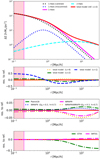 |
Fig. 2. Differencial surface density profile model as a function of radius. Upper panel: model of the projected excess of surface mass density as a function of the comoving radial distance from the centre for a cluster with M200 = 1014 M⊙ h−1, c200 = 3 at redshift z = 0.3, with σoff = 0.3 and foff = 0.3. The radius enclosing 200 times the critical density corresponds to R200 = 1.47 Mpc h−1. The four one-halo and two-halo terms are shown with different colours and styles, as labelled. Second panel: relative differences, with respect to the reference, of the models with rt = 1, 2, and 4. Third panel: relative differences, with respect to the reference, of the models with the linear power spectrum estimated assuming different cosmological model parameters, as labelled. Shown for comparison (yellow dotted curve) is the relative difference between the prediction adopting WMAP9 cosmology and WMAP9, but fixing ΩM = 0.3 and h = 0.7. Bottom panel: relative differences, with respect to the reference, of two models constructed with either the Sheth & Tormen (1999) or the Sheth et al. (2001) biasing model. |
4. Results
In this section we present the main results of our analysis. Firstly, we model the small-scale stacked surface mass density profiles, assessing the structural properties of the hosting halo population. Then we model the full lensing signal up to the largest available scales, constraining the total matter density parameter, ΩM.
In the first part of our analysis, when modelling the small-scale signal coming from the central part of the clusters only, we limit the analysis to scales between 0.2 and 3.16 Mpc h−1. We refer to this as the ∼1h case since most of the contribution to the measured signal comes from the main dark matter haloes hosting the galaxy clusters. As the upper panel of Fig. 2 shows, the two-halo term affects, to a small degree, only the last few radial bins available. This makes our inference on the cluster halo structural properties, expressed in terms of the four one-halo (NFW) model parameters (M200, c200, foff, and σoff), much less dependent on the uncertain details of the halo biasing model. To test this assumption, we repeated the following analysis including only the one-halo contribution, finding that the mass is slightly overestimated by a few percentage points (see Table 1 for more details). For each corresponding case, in parentheses we report the χ2 divided by the number of degrees of freedom (d.o.f.). We recall that the highest S/N comes from small-scale lensing in this kind of measurements, but it may be affected by both theoretical and observational systematic uncertainties (Mandelbaum et al. 2013).
Subsequently, we model the total stacked density profiles up to 35 Mpc h−1. In this case we consider Gaussian priors on the four parameters of the one-halo term, with the mean and the standard deviation corresponding to the posterior distribution results. The main goal here is to derive constraints on ΩM marginalised over the parameters of the one-halo term. We refer to this cosmological analysis as the 1h + 2h case.
4.1. Constraining the cluster structural properties
In this section we model the stacked shear profiles collected in the 0.2 < R < 3.16 Mpc h−1 radial range, while in the next section we exploit the profiles measured up to 35 Mpc h−1, where the two-halo term contribution dominates. In both cases we bin the dataset adopting a logarithmic binning along the radial directions, choosing dlog(r) ≈ 0.1 we have 14 and 30 radial bins for the two cases, ∼1h and 1h + 2h, respectively. In both cases the analyses are based on a set of 14 stacked excess surface density profiles of clusters, obtained by dividing the whole AMICO-KiDS-DR3 cluster catalogue in redshift and amplitude, as reported in the first four columns of Table 1.
In order to properly model the large-scale weak lensing signal we need to take into account most of the systematics and uncertainties that could emerge in the very weak regime where the excess surface mass density becomes low. We perform this by constructing stacked profiles around random positions in different redshift bins, which we subtract from the stacked cluster profiles (Sereno et al. 2018; Bellagamba et al. 2019). We generate 10 000 realisations of a sample of 6962 random positions properly accounting for the KiDS-DR3 survey masks (Fig. 1) and the cluster redshift distribution. The number of random realisations was selected as a good compromise between the computational cost needed for the analyses and the number of AMICO clusters used in this work. In Fig. 3 we display the excess surface mass density profiles around the random centres for the three different redshift ranges considered, and for the average profile (for simplicity we exhibit only the dataset for the 1h + 2h case). The error bars are the square root of the diagonal terms of the corresponding covariances CRandoms(r, r′) computed by constructing the excess surface mass density around random centres,

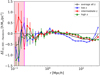 |
Fig. 3. Excess of surface mass density profile around random centres for the three redshift bins into which the AMICO clusters have been divided: low (0.1 ≤ z < 0.3), intermediate (0.3 ≤ z < 0.45), and high (0.45 ≤ z ≤ 0.6) redshift. We created 10 000 realisations of the sample using random centres. The blue crosses, red diamonds, and green triangles show the average measurements in the three redshift intervals, extending the profiles up to 35 Mpc h−1 as in the 1h + 2h case. The black line displays the average over all redshifts. The error bars show square root of the diagonal terms of the corresponding covariances CRandoms(r, r′). The vertical pink area on the left gives the data points below 0.2 Mpc h−1, which we do not consider in our analysis. |
where  indicates the average profile over the considered random dataset. All the average profiles are consistent with zero, showing only a mild deviation at large distances, due to the survey masks.
For the cluster stacked surface mass density profile we compute the covariance matrix C(r, r′) for each of the amplitude and redshift bins using 10 000 bootstrap realisations. As an illustrative case, in the left panel of Fig. 4 we display the normalised covariance matrix for one of the bins, specifically the bin with 0.1 ≤ z < 0.3 and 2.05 ≤ A < 2.75, that contains 96 clusters. The central panel of Fig. 4 shows the normalised ΔΣ covariance computed generating 10 000 times the AMICO-KiDS-DR3 cluster sample, but assigning random positions in the KiDS-DR3 field of view. We note that the off-diagonal term contributions in this case are almost negligible, which allows us to compute the final covariance CC(r, r′) for the stacked excess surface mass density profiles, in each redshift and amplitude bin by summing in quadrature only the diagonal terms
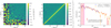 |
Fig. 4. Example of covariances and differencial surface density profiles. Left panel: normalised covariance of the dataset corresponding to the bin with 0.1 ≤ z < 0.3 and 2.05 ≤ A < 2.75, stacking 96 detected clusters, computed with 10 000 bootstrap realisations of the stacked profile. Central panel: normalised covariance of the 10 000 realisations of the whole AMICO sample, randomly distributed in the survey footprints. Right panel: stacked excess surface mass density profile of the 1h case (blue crosses) and 1h + 2h case (orange circles). In both cases we subtract to the data points the stacked profiles around random centre. The error bars refer to the square root of the diagonal elements of the final covariance (Eq. (17)). The red arrows indicate the variation of the stacked profile when, for the corresponding redshift bin, the random contributions are subtracted from the data. The blue crosses and orange filled circles refer to two different binning schemes, giving the possibility to constrain the cluster-halo structural properties and the large-scale matter density distribution in which the clusters are located, respectively. |
with nRandoms = 10 000 and δ(r, r′) the 2D delta Dirac function, which is equal to one for r = r′ and zero otherwise. The right panel of Fig. 4 shows the stacked ΔΣ profile around the 96 clusters considered sample. The blue crosses (orange circles) display the ∼1h case (1h + 2h case), where the profiles are constructed adopting 14 (30) radial bins up to 3.16 Mpc h−1 (30 Mpc h−1) minus the corresponding profiles around 10 000 random centre. The error bars represent the square root of the diagonal term of the final covariance CC(r, r′). As an example, the red arrows, corresponding to each orange circle point, indicate the variation of the ΔΣ profile. In our analysis, performed adopting the CosmoBolognaLig (Marulli et al. 2016), we numerically invert the covariance matrix using the GSL3 library.
Figure 4 shows that the random contribution on small scales is negligible, while it becomes relatively important on large scales when ΔΣ is smaller than 10 h M⊙ pc−2. This justifies the choice by Bellagamba et al. (2019) not to correct for this effect in their small-scale analysis.
Figure 5 shows stacked excess surface mass density profiles of the AMICO-KiDS-DR3 clusters, divided into different amplitude and redshift ranges. The blue and orange data points refer to the ∼1h and 1h + 2h dataset cases, respectively. From both cases we subtract the contributions around random centres. The matching error bars display the square root of the diagonal terms in the covariance matrix. The blue and red solid curves show the best-fit models, the median values of the posterior distributions assessed with the MCMC, corresponding to the ∼1h and 1h + 2h cases, respectively. In running our MCMC on the ∼1h case dataset, we adopt uniform priors for the four structural properties parameters:
-
log(M200/h−1 M⊙): [12.5−15.5];
-
c200: [1−20];
-
foff: [0−0.5];
-
σoff/h−1 Mpc: [0−0.5].
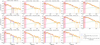 |
Fig. 5. Stacked excess surface mass density profiles of the clusters divided in different amplitude bins (from left to right) and redshift bins (from top to bottom). The blue and orange data points refer to the ∼1h and 1h + 2h cases, respectively. The corresponding error bars represent the square root of the diagonal terms in the corresponding covariance matrix. The blue and red solid curves show the best-fit models, which are the median values of the posterior distributions assessed with the MCMC, corresponding to the ∼1h and 1h + 2h cases, respectively. The blue and red curves are respectively dotted and dashed outside the corresponding dataset, especially the blue line below 0.2 and above 3.16 Mpc h−1, and the red line only below 0.2 Mpc h−1. The green curves show the two-halo term contribution. |
4.2. Scaling relations
In Fig. 6 we show the weak lensing mass-amplitude relation obtained in this work from the small-scale analysis (∼1h case), compared to previous analysis performed on the same dataset. Moreover, we model the trend using a linear relation between the photometric observable and the recovered mass, as also discussed by Sereno & Ettori (2015) and Bellagamba et al. (2019),
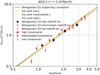 |
Fig. 6. Mass-amplitude relation obtained in the ∼1h case, accounting for the full covariance in each amplitude and redshift interval. We compare our results (red data points) with those by Bellagamba et al. (2019) (black data points). The error bars show the 18th and 82nd percentiles of the posterior distributions. The blue solid line shows the scaling relation recovered by Bellagamba et al. (2019); the orange solid line exhibits our best-fit result. |
where we set Apiv = 2, zpiv = 0.35, as in Bellagamba et al. (2019), and E(z) = H(z)/H0. We recall that, differently from Bellagamba et al. (2019), we subtract the redshift stacked profiles around random centres and account for the full covariance matrix in our MCMC analysis. The red data points display the median results of our analysis, while the error bars show the 18th and 82nd percentiles of the posterior distributions. The black data points exhibit the original results from Bellagamba et al. (2019), which show a reasonable agreement with our results, within the error bars. It should be noted in Fig. 6 that by accounting for the full covariance in our MCMC analysis we obtain slightly smaller masses, and thus the slope of our linear relations (orange lines) is slightly shallower than the one derived by Bellagamba et al. (2019) (blue lines); we display the relation neglecting the redshift evolution in order to avoid overcrowding the figure. We performed our analysis accounting only for the 1h term in the modelling function and adopting different cases for the truncation radius. In particular, we discuss in Appendix A the results adopting different truncation radii.
In Fig. 7 we display the posterior distributions of the mass-amplitude model parameters (Eq. (18)), obtained by modelling the red data points, and their corresponding error bars, shown in Fig. 6.
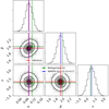 |
Fig. 7. Posterior distributions of the parameters of the mass-amplitude relation in Eq. (18). The contours show the 68th and 95th percentiles of the distributions. For comparison, also shown are the results for α, β, and γ obtained by Bellagamba et al. (2019) (green squares) and when assuming a flat WMAP9 cosmology, fixing ΩM = 0.3 and h = 0.7. |
We follow the same fitting procedure adopted in Bellagamba et al. (2019), where the amplitude is computed through a lensing-weighted average. Moreover, we account for the systematic errors in the covariance by summing in quadrature the uncertainties for background selection, photo-zs, and shear measurements (Bellagamba et al. 2019; Sereno et al. 2020). We assume uniform priors in the ranges −1 < α < 1, 0.1 < β < 5, and −5 < γ < 54. The obtained median values of the posterior distributions of the mass-amplitude relation parameters, and the 18th and 82nd percentiles around them, are summarised in Table 2. In the second line of the table we also report the scaling relation parameters for the masses estimated on the ∼1h case dataset, but adopting in the modelling function only the 1h term. In this case we note that the slight overestimate of the masses drives the scaling relation towards a steeper value. We recall Table 1, where we display the median mass (expressed in term of the logarithm in base 10) of the posterior distributions for the various cases considered; the values reported in parentheses show the χ2 divided by the number of d.o.f.
Scaling relation parameters of the mass-amplitude relation.
The contours in Fig. 7 display the 68th and 95th percentiles of the posterior distributions. For comparison, we show also the best-fit results obtained adopting a different parametrisation of the matter power spectrum in the two-halo term (flat-WMAP9 parameters, but with ΩM = 0.3 and h = 0.7), and the results by Bellagamba et al. (2019). All results shown in Fig. 7 appear statistically consistent. We also note that the adoption of a flat Planck18 or WMAP9 cosmology, fixing ΩM = 0.3 and h = 0.7, impacts mainly the modelling of the 2h term, which is negligible when analysing the ∼1h case data up to 3.16 Mpc h−1.
As explained in Sect. 3.1, the one-halo model used in this analysis has four free parameters: foff and σoff parametrise the uncertainty relative to the cluster centre definition, and M200 and c200 are related to the halo structural properties. Theoretical models (Eke et al. 2001; Zhao et al. 2009; Ludlow et al. 2012) and numerical simulations (Dolag et al. 2004; Neto et al. 2007; Macciò et al. 2008; Duffy et al. 2008; Klypin et al. 2016) predict that, at fixed redshift, the halo concentration is a decreasing function of the halo mass. Less massive haloes forming at higher redshifts tend to be more concentrated than the more massive ones (van den Bosch 2002; Wechsler et al. 2002); cluster-sized haloes are still in their formation phase.
In Fig. 8 we display the concentration-mass relation for our stacked cluster sample in the three redshift bins considered, compared to the theoretical predictions for our reference cosmological model adopting the Zhao et al. (2009) recipe, where the concentration is related to the time at which haloes assemble 4% of their mass. To follow the mass accretion histories of the haloes back in time, we use the model by Giocoli et al. (2012a). We perform a log-log linear regression modelling the 14 data points5, though the small number of data points does not allow us to constrain the redshift dependence of this relation.
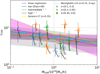 |
Fig. 8. Concentration-mass relation obtained from our stacked weak lensing analysis of the AMICO-KiDS-DR3 clusters. Data points and error bars show the median and the 18th−82th percentiles of the posteriors distributions. Blue, orange and green colours refer to the low, intermediate and high redshift cluster sub-samples. The solid curves represent the predictions by Zhao et al. (2009) in three redshift intervals. For each data point, the numbers show the results for the c − M relation obtained adopting the truncation radius rt equal to 1, 2 and 4 – in unit of R200, respectively. The grey and light-grey shaded regions indicate 1 and 2-σln c = 0.25 scatter as measured in numerical simulations (Dolag et al. 2004; Giocoli et al. 2012a). The magenta line show the linear regression in the c − m relation computed using our reference results as dataset, while the shaded light-magenta region encloses the 1-σ uncertainties in both the slope and the intercept of the relation. In this case, we use the ODR routine in python considering the uncertainties in both mass and concentration. Dashed gold and dash-dotted cyan display the results by Sereno et al. (2017) – based on observational data – and Meneghetti et al. (2014) – on hydrodynamical simulations, respectively. |
The log−log linear relation obtained from the fitting analysis is

with B = −0.22 ± 0.21 and C = 0.74 ± 0.08, which is in good agreement with the results from numerical simulations (Duffy et al. 2008; Prada et al. 2012; Ludlow et al. 2014; Meneghetti et al. 2014) and from observational data in the corresponding mass ranges (Mandelbaum et al. 2008; Merten 2016; Sereno et al. 2017). The shaded light magenta region in Fig. 8 encloses the 1σ uncertainties in both the slope and the intercept of the relation. For comparison and for each data point, the numbers exhibit the results for the c200 − M200 relation obtained adopting the truncation radius rt equal to 1, 2, and 4 in units of R200. In the figure we also display the finding by Sereno et al. (2017), who modelled the relation of the PSZ2LenS clusters, and the results by Meneghetti et al. (2014), who fit the results of hydrodynamical simulations for the 2D fit of the X-ray selected cluster sample. Both relations refer to an intermediate redshift of our cluster sample corresponding to z = 0.35.
4.3. Constraining the total matter density parameter
In this section we present the results when modelling the large-scale ΔΣ profiles up to 35 Mpc h−1, 1h + 2h case. The large-scale signal is sensitive to the linear power spectrum normalisation and to the host halo bias (Sereno et al. 2015, 2017, 2018). In this work we follow the approach of fixing the halo bias–cluster mass relation, and its redshift dependence, to the results obtained from the analyses of various numerical simulations (Sheth & Tormen 1999; Sheth et al. 2001; Tinker et al. 2010), while leaving the matter density parameter ΩM as a free quantity to vary in our analysis. The σ8 parameter, measuring the power spectrum fluctuations smoothed with a top-hat window function of aperture 8 Mpc h−1, are obtained as a derived quantity from our MCMC and the corresponding cosmological model.
We employ the same Bayesian approach and the 1h + 2h modelling function used in the previous section, introducing an extra d.o.f., that is the total matter density parameter ΩM, assuming a flat Universe (i.e. ΩΛ = 1 − ΩM). In doing so, we consistently account for the cosmology dependence of the conversion from angular to comoving and physical coordinate in our dataset (i.e. the radial profiles of ΔΣ). The stacked weak lensing profiles shown above were computed assuming a reference flat cosmology with ΩM = 0.3 and h = 0.7. In the Bayesian analysis, when varying the matter density parameter, we take into account the dependence on ΩM not only on r, but also on ΔΣ (see Eq. (5)).
The red curves shown in Fig. 5 display the best-fit models computed from the MCMC Bayesian analysis, corresponding to the median values of the posterior distributions. As described in Sect. 3.2 and above, the considered model has five free parameters: M200, c200, foff, σoff, and ΩM. In modelling the 1h + 2h case dataset we assume Gaussian priors for the four one-halo model parameters with mean and standard deviation corresponding to the 1h case modelling posteriors, while we let ΩM vary between 0.06 and 0.6, uniformly (see Table 3). The corresponding two-halo term contribution are also shown.
Priors considered in the various redshift and amplitude bins.
In our analyses there were two reasons for performing this twofold approach (first performing the fit of the halo structural property parameters, and then, while limiting them to a smaller Gaussian interval, constraining the total matter density parameter). The first reason is related to the wide range of scales probed by our stacked weak lensing profiles, and the second is connected to the number of parameters that we vary, four for the one-halo term and one for the two-halo. Our procedure allows the weights of the small and large scale contributions to be separated in a self-consistent way.
Figure 9 displays the relation between the recovered weak lensing mass and total matter density parameter ΩM. From the figure we note that there is no particular correlation. The data points display the medians and the error bars give the 18th and 82nd percentiles of the posterior distributions. The different coloured data points refer to the three redshift ranges considered. Shown are the weighted average of the various ΩM estimates and its associated uncertainty. The last line of Table 2 displays the mass-amplitude relation parameters (see Eq. (18)) obtained modelling the 1h + 2h case dataset.
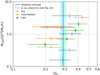 |
Fig. 9. Correlation between the recovered cluster mass and total matter density parameter from our stacked weak lensing analysis. The different coloured data points refer to three redshift ranges considered (see legend, top left corner). The blue solid line displays the weighted average of the various estimated ΩM for the different amplitude and redshift bins; the cyan shaded region encloses the 1σ uncertainty. The dashed red line gives the weighted average of the posterior distributions, as in Fig. 10. |
As discussed in Sect. 3 we assumed Planck18 as the reference cosmological model, but fixing ΩM = 0.3 and h = 0.7, since the distances and the stacked weak lensing data were computed assuming those parameters (Bellagamba et al. 2019). In Fig. 10 we show the posterior distributions for the measured ΩM parameter in the three redshift bins considered, as well as the result obtained by combining all redshifts together. In this case we fixed all the cosmological parameters to the flat Planck18 values, varying only ΩM uniformly in the range [0.06−0.6]. The one-halo term parameters are varied in the same range as was used for the ∼1h case dataset, but assuming a Gaussian distribution for the priors with mean and standard deviation as for the ∼1h case posteriors. The posterior distribution of ΩM from the analysis of the CMB data performed by the Planck Collaboration VI (2020) is shown. In the figure we note a small shift towards lower values of ΩM for the intermediate redshift bin; however, it is consistent with the other redshift intervals within the measured uncertainties. As noted by Maturi et al. (2019), this interval may suffer from slightly larger photometric errors that could impact the modelling of the estimated tangential shear profile; we expect to investigate this further in the next AMICO-KiDS data release.
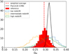 |
Fig. 10. Posterior distributions of the total matter density parameter ΩM. The blue, orange, and green histograms show the results for the low, intermediate, and high redshift cluster samples, respectively. The red-filled histogram exhibits the posterior distribution combining all redshifts together; the dashed red line indicates the median of the distribution. The black curve displays the posterior distribution obtained from the analysis of the CMB data by Planck Collaboration VI (2020). |
Table 4 reports the ΩM constraints obtained from the stacked weak lensing analyses for the three redshift ranges considered, and the combined redshifts.
Constraints on ΩM obtained from the stacked weak lensing analyses at the three redshift ranges considered, and the combined redshifts.
In our cosmological analysis, we are in good agreement with Lesci et al. (2020) and Nanni et al. (in prep.) who analysed the same AMICO-KiDS-DR3 dataset. This is remarkable since our analysis is independent from cluster-clustering and cluster-counts, but we still find a consistent value of ΩM.
We discuss the model systematics of our results in greater detail in the two appendices. In Appendix A we examine the impact of the truncation radius in modelling the ∼1h case, while in Appendix B we discuss the impact of recovering the total matter density parameter (modelling the 1h + 2h case dataset) and of using a different reference linear power spectra and various halo bias models.
5. Summary and conclusions
In this work we presented new cosmological results from the analysis of weak lensing signal produced by a galaxy cluster sample detected from the KiDS-DR3 survey (de Jong et al. 2017; Hildebrandt et al. 2017). Specifically, we exploited photometric redshifts with relative probability distribution functions (Kuijken et al. 2015; de Jong et al. 2017), a global improved photometric calibration, weak lensing shear catalogues (Kuijken et al. 2015; Hildebrandt et al. 2017), and lensing-optimised image data. Our cluster sample, used to build the stacked shear profiles for the cosmological analysis, was obtained using the AMICO algorithm (Bellagamba et al. 2018) in Maturi et al. (2019). The redshift-amplitude binning of the cluster sample was constructed as in Bellagamba et al. (2019).
Our studies support the use of the stacking method in weak lensing to calibrate galaxy cluster scaling relations, in agreement with previous results. The robustness of the AMICO-KiDS-DR3 dataset enabled us to infer cosmological parameters from the stacked shear measurements. Modelling the shear profiles of these clusters up to large scales, we inferred robust cosmological constraints on ΩM, assuming a reference recipe for the halo bias parameter (Tinker et al. 2010).
We constructed two datasets from the same cluster and galaxy shear catalogues. The first dataset was used for the ∼1h case analysis in which we binned the stacked radial excess surface mass density profiles in 14 intervals from 0.1 to 3.16 Mpc h−1, as in Bellagamba et al. (2019), while the second dataset was considered for the 1h + 2h case where the analyses were performed in 30 bins up to 35 Mpc h−1. In order to keep all the observational systematic uncertainties of the survey under control, we subtracted the signal around random centres from the measurements, randomising 10 000 times the positions of the 6962 AMICO clusters. We also accounted for the full covariances on the final ΔΣ profiles. We split our datasets into 14 stacked measures in redshift and amplitude. We used a halo model approach developed in our MCMC routines in the CosmoBolognaLib (Marulli et al. 2016). Modelling the ∼1h case dataset, we recovered with good accuracy the cluster halo structural model parameters (M200, c200, foff, σoff) and the mass-amplitude relation parameters. We also studied the impact of adopting only the 1h term in our modelling function, finding a small positive bias in mass of the order of a few percent. In addition, we modelled the recovered concentration and mass relation of the 14 samples finding very good agreement with other observational studies and numerical simulation results: more massive haloes tend to be less concentrated than the smaller ones. However, the small dataset and the mild expected redshift dependence of the relation does not allow us to model the redshift evolution of the c200 − M200 relation.
We employed the 1h + 2h case dataset to simultaneously constrain the cluster structural properties and the ΩM parameter. Our results are fully consistent with the theoretical predictions of the ΛCDM model. Marginalising over the cluster model parameters, we obtained ΩM = 0.29 ± 0.02 from the combined posterior distribution, assuming a flat geometry. This value is fully consistent with the independent results on the same cluster sample performed by Lesci et al. (2020) and Nanni et al. (in prep.), and also in agreement with the findings from recent CMB experiments (Bennett et al. 2013; Planck Collaboration VI 2020): higher than the low value of the total matter density parameter estimated from counts and weak lensing signal of redMaPPer clusters from the Dark Energy Survey (DES) Year 1 (Abbott et al. 2020), and slightly lower than the value computed by Planck Collaboration VI (2020) analysing CMB data.
We expect to reduce the uncertainties on our finding by enhancing the number of clusters to stack, looking forward to the new cluster catalogues from the future KiDS data releases, and afterwards from the data coming from future wide field surveys like the ESA-Euclid mission (Laureijs et al. 2011). Upcoming deeper galaxy surveys will allow us to detect and stack lensing clusters in small redshift bins and to extend the analysis up to higher redshifts, enabling us to break parameter degeneracies and limit systematic uncertainties (Oguri & Takada 2011). The accuracy in the estimate of cosmological parameters will significantly benefit from the advancements planned for KiDS when it will reach its final coverage of 1350 deg2 of sky, with a median redshift of ∼0.8.
The lensing signal can be incremented by considering a larger number of clusters (which can be attained with either deeper or wider surveys) and background sources (deeper surveys), and a wider survey area, in order to collect the two-halo term lensing signal up to 50 Mpc h−1. These aspects will be reached by the ESA-Euclid mission, which will provide a significantly improved dataset compared to the one used in this work. The Euclid Wide Survey is expected to cover an area of ∼15 000 deg2 and it will detect approximately ng ∼ 30 galaxies per square arcminute, with a median redshift larger than 0.9.
We conclude by noting that our methodology of finding clusters, and our cosmological statistical analyses in modelling the weak lensing shear profiles around them, will represent a reference starting point and a milestone for cluster cosmology in near future experiments.
The data products that constitute the main DR3 release (stacked images, weight and flag maps, and single-band source lists for 292 survey tiles, as well as a multi-band catalogue for the combined DR1, DR2, and DR3 survey area of 440 survey tiles) are released via the ESO Science Archive, and they are also accessible via the Astro-WISE system (http://kids.strw.leidenuniv.nl/DR1/access_aw.php) and the KiDS website http://kids.strw.leidenuniv.nl/DR3.
The method used to assess the quality of the detections exploits realistic mock catalogues constructed from the real data themselves, as described in Sect. 6.1 of Maturi et al. (2019). These mock catalogues are used to estimate the uncertainties on the quantities characterising the detections, as well as the purity and completeness of the entire sample.
We use emcee for this fitting analysis, https://emcee.readthedocs.io/en/stable
The fitting analysis is done with the Orthogonal Distance Regression routine https://docs.scipy.org/doc/scipy/reference/odr.html, accounting for the uncertainties on both mass and concentration.
Acknowledgments
Based on data products from observations made with ESO Telescopes at the La Silla Paranal Observatory under programme IDs 177.A-3016, 177.A-3017 and 177.A-3018, and on data products produced by Target/OmegaCEN, INAF-OACN, INAF-OAPD and the KiDS production team, on behalf of the KiDS consortium. OmegaCEN and the KiDS production team acknowledge support by NOVA and NWO-M grants. Members of INAF-OAPD and INAF-OACN also acknowledge the support from the Department of Physics and Astronomy of the University of Padova, and of the Department of Physics of Univ. Federico II (Naples). We acknowledge the KiDS Collaboration for the public data realises and the various scientists working within it for the fruitful and helpful discussions. We acknowledge the grants ASI n.I/023/12/0, ASI-INAF n. 2018-23-HH.0 and PRIN MIUR 2015 “Cosmology and Fundamental Physics: illuminating the Dark Universe with Euclid”. CG and LM are also supported by PRIN-MIUR 2017 WSCC32 “Zooming into dark matter and proto-galaxies with massive lensing clusters”. CG acknowledges support from the Italian Ministry of Foreign Affairs and International Cooperation, Directorate General for Country Promotion. MS acknowledges financial contribution from contract ASI-INAF n.2017-14-H.0 and contract INAF mainstream project 1.05.01.86.10. JHD acknowledges support from an STFC Ernest Rutherford Fellowship (project reference ST/S004858/1). We thank the reviewer for her/his useful comments that helped us to improve the presentation of our results. All authors have contributed to the scientific preparation of this work. Particularly: CG leads the paper preparing the dataset, performing the computational analyses, and organising the manuscript; FM, LM, MS, AV, and LG helped with the development of some codes and the scientific interpretation of the results; MM, MR, FB, and MR implemented the code for cluster detection and lead the first lensing analyses of the same dataset; SB, SC, GC, JHD, LI, GL, LN, and EP participated in the discussion and interpretation of the results. The authors acknowledge the use of computational resources from the parallel computing cluster of the Open Physics Hub (https://site.unibo.it/openphysicshub/en) at the Physics and Astronomy Department in Bologna.
References
- Abbott, T. M. C., Aguena, M., Alarcon, A., et al. 2020, Phys. Rev. D, 102, 023509 [CrossRef] [Google Scholar]
- Andreon, S. 2010, MNRAS, 407, 263 [NASA ADS] [CrossRef] [Google Scholar]
- Angelinelli, M., Vazza, F., Giocoli, C., et al. 2020, MNRAS, 495, 864 [CrossRef] [Google Scholar]
- Angulo, R. E., Springel, V., White, S. D. M., et al. 2012, MNRAS, 426, 2046 [CrossRef] [Google Scholar]
- Baltz, E. A., Marshall, P., & Oguri, M. 2009, JCAP, 2009, 015 [Google Scholar]
- Bartelmann, M., & Schneider, P. 2001, Phys. Rep., 340, 291 [NASA ADS] [CrossRef] [Google Scholar]
- Bautista, J. E., Paviot, R., Vargas Magaña, M., et al. 2021, MNRAS, 500, 736 [Google Scholar]
- Bellagamba, F., Maturi, M., Hamana, T., et al. 2011, MNRAS, 413, 1145 [NASA ADS] [CrossRef] [Google Scholar]
- Bellagamba, F., Roncarelli, M., Maturi, M., & Moscardini, L. 2018, MNRAS, 473, 5221 [NASA ADS] [CrossRef] [Google Scholar]
- Bellagamba, F., Sereno, M., Roncarelli, M., et al. 2019, MNRAS, 484, 1598 [NASA ADS] [CrossRef] [Google Scholar]
- Benítez, N. 2000, ApJ, 536, 571 [Google Scholar]
- Bennett, C. L., Larson, D., Weiland, J. L., et al. 2013, ApJS, 208, 20 [Google Scholar]
- Borgani, S., & Kravtsov, A. 2011, Adv. Sci. Lett., 4, 204 [CrossRef] [Google Scholar]
- Borgani, S., Murante, G., Springel, V., et al. 2004, MNRAS, 348, 1078 [Google Scholar]
- Cacciato, M., van den Bosch, F. C., More, S., et al. 2009, MNRAS, 394, 929 [NASA ADS] [CrossRef] [Google Scholar]
- Cacciato, M., Lahav, O., van den Bosch, F. C., Hoekstra, H., & Dekel, A. 2012, MNRAS, 426, 566 [NASA ADS] [CrossRef] [Google Scholar]
- Capaccioli, M., & Schipani, P. 2011, The Messenger, 146, 2 [NASA ADS] [Google Scholar]
- Costanzi, M., Rozo, E., Simet, M., et al. 2019, MNRAS, 488, 4779 [NASA ADS] [CrossRef] [Google Scholar]
- de Jong, J. T. A., Verdoes Kleijn, G. A., Kuijken, K. H., & Valentijn, E. A. 2013, Exp. Astron., 35, 25 [Google Scholar]
- de Jong, J. T. A., Verdoes Kleijn, G. A., Boxhoorn, D. R., et al. 2015, A&A, 582, A62 [NASA ADS] [CrossRef] [EDP Sciences] [Google Scholar]
- de Jong, J. T. A., Verdoes Kleijn, G. A., Erben, T., et al. 2017, A&A, 604, A134 [NASA ADS] [CrossRef] [EDP Sciences] [Google Scholar]
- Dolag, K., Bartelmann, M., Perrotta, F., et al. 2004, A&A, 416, 853 [NASA ADS] [CrossRef] [EDP Sciences] [Google Scholar]
- Duffy, A. R., Schaye, J., Kay, S. T., & Dalla Vecchia, C. 2008, MNRAS, 390, L64 [NASA ADS] [CrossRef] [Google Scholar]
- Eisenstein, D. J., & Hu, W. 1999, ApJ, 511, 5 [NASA ADS] [CrossRef] [Google Scholar]
- Eke, V. R., Navarro, J. F., & Steinmetz, M. 2001, ApJ, 554, 114 [NASA ADS] [CrossRef] [Google Scholar]
- Fenech Conti, I., Herbonnet, R., Hoekstra, H., et al. 2017, MNRAS, 467, 1627 [NASA ADS] [Google Scholar]
- George, M. R., Leauthaud, A., Bundy, K., et al. 2012, ApJ, 757, 2 [NASA ADS] [CrossRef] [Google Scholar]
- Giocoli, C., Bartelmann, M., Sheth, R. K., & Cacciato, M. 2010, MNRAS, 408, 300 [NASA ADS] [CrossRef] [Google Scholar]
- Giocoli, C., Tormen, G., & Sheth, R. K. 2012a, MNRAS, 422, 185 [NASA ADS] [CrossRef] [Google Scholar]
- Giocoli, C., Meneghetti, M., Bartelmann, M., Moscardini, L., & Boldrin, M. 2012b, MNRAS, 421, 3343 [Google Scholar]
- Giocoli, C., Meneghetti, M., Metcalf, R. B., Ettori, S., & Moscardini, L. 2014, MNRAS, 440, 1899 [NASA ADS] [CrossRef] [Google Scholar]
- Hamana, T., Shirasaki, M., Miyazaki, S., et al. 2020, PASJ, 72, 16 [CrossRef] [Google Scholar]
- Hennig, C., Mohr, J. J., Zenteno, A., et al. 2017, MNRAS, 467, 4015 [NASA ADS] [Google Scholar]
- Heymans, C., Van Waerbeke, L., Miller, L., et al. 2012, MNRAS, 427, 146 [NASA ADS] [CrossRef] [Google Scholar]
- Hikage, C., Oguri, M., Hamana, T., et al. 2019, PASJ, 71, 43 [NASA ADS] [CrossRef] [Google Scholar]
- Hildebrandt, H., Erben, T., Kuijken, K., et al. 2012, MNRAS, 421, 2355 [Google Scholar]
- Hildebrandt, H., Viola, M., Heymans, C., et al. 2017, MNRAS, 465, 1454 [Google Scholar]
- Johnston, D. E., Sheldon, E. S., Wechsler, R. H., et al. 2007, ArXiv e-prints [arXiv:0709.1159] [Google Scholar]
- Klypin, A., Yepes, G., Gottlober, S., Prada, F., & Hess, S. 2016, MNRAS, 457, 4340 [NASA ADS] [CrossRef] [Google Scholar]
- Kuijken, K. 2011, The Messenger, 146, 8 [NASA ADS] [Google Scholar]
- Kuijken, K., Heymans, C., Hildebrandt, H., et al. 2015, MNRAS, 454, 3500 [Google Scholar]
- Laureijs, R., Amiaux, J., Arduini, S., et al. 2011, ArXiv e-prints [arXiv:1110.3193] [Google Scholar]
- Lesci, G. F., Marulli, F., Moscardini, L., et al. 2020, A&A, submitted [arXiv:2012.12273] [Google Scholar]
- Lewis, A., Challinor, A., & Lasenby, A. 2000, ApJ, 538, 473 [Google Scholar]
- Liske, J., Baldry, I. K., Driver, S. P., et al. 2015, MNRAS, 452, 2087 [NASA ADS] [CrossRef] [Google Scholar]
- LSST Science Collaboration (Abell, P. A., et al.) 2009, ArXiv e-prints [arXiv:0912.0201] [Google Scholar]
- Ludlow, A. D., Navarro, J. F., Li, M., et al. 2012, MNRAS, 427, 1322 [NASA ADS] [CrossRef] [Google Scholar]
- Ludlow, A. D., Navarro, J. F., Angulo, R. E., et al. 2014, MNRAS, 441, 378 [NASA ADS] [CrossRef] [Google Scholar]
- Macciò, A. V., Dutton, A. A., van den Bosch, F. C., et al. 2007, MNRAS, 378, 55 [NASA ADS] [CrossRef] [Google Scholar]
- Macciò, A. V., Dutton, A. A., & van den Bosch, F. C. 2008, MNRAS, 391, 1940 [NASA ADS] [CrossRef] [Google Scholar]
- Mandelbaum, R., Hirata, C. M., Ishak, M., Seljak, U., & Brinkmann, J. 2006, MNRAS, 367, 611 [NASA ADS] [CrossRef] [Google Scholar]
- Mandelbaum, R., Seljak, U., & Hirata, C. M. 2008, JCAP, 2008, 006 [NASA ADS] [CrossRef] [Google Scholar]
- Mandelbaum, R., Slosar, A., Baldauf, T., et al. 2013, MNRAS, 432, 1544 [NASA ADS] [CrossRef] [Google Scholar]
- Marulli, F., Veropalumbo, A., & Moresco, M. 2016, Astron. Comput., 14, 35 [Google Scholar]
- Marulli, F., Veropalumbo, A., Sereno, M., et al. 2018, A&A, 620, A1 [NASA ADS] [CrossRef] [EDP Sciences] [Google Scholar]
- Marulli, F., Veropalumbo, A., García-Farieta, J. E., et al. 2020, ApJ, submitted [arXiv:2010.11206] [Google Scholar]
- Maturi, M., Meneghetti, M., Bartelmann, M., Dolag, K., & Moscardini, L. 2005, A&A, 442, 851 [NASA ADS] [CrossRef] [EDP Sciences] [Google Scholar]
- Maturi, M., Schirmer, M., Meneghetti, M., Bartelmann, M., & Moscardini, L. 2007, A&A, 462, 473 [NASA ADS] [CrossRef] [EDP Sciences] [Google Scholar]
- Maturi, M., Bellagamba, F., Radovich, M., et al. 2019, MNRAS, 485, 498 [Google Scholar]
- Meneghetti, M., Rasia, E., Merten, J., et al. 2010, A&A, 514, A93 [NASA ADS] [CrossRef] [EDP Sciences] [Google Scholar]
- Meneghetti, M., Rasia, E., Vega, J., et al. 2014, ApJ, 797, 34 [Google Scholar]
- Merten, J. 2016, MNRAS, 461, 2328 [NASA ADS] [CrossRef] [Google Scholar]
- Miller, L., Kitching, T. D., Heymans, C., Heavens, A. F., & van Waerbeke, L. 2007, MNRAS, 382, 315 [Google Scholar]
- Miller, L., Heymans, C., Kitching, T. D., et al. 2013, MNRAS, 429, 2858 [Google Scholar]
- Mo, H. J., & White, S. D. M. 1996, MNRAS, 282, 347 [Google Scholar]
- Moresco, M., Veropalumbo, A., Marulli, F., Moscardini, L., & Cimatti, A. 2020, ApJ, submitted [arXiv:2011.04665] [Google Scholar]
- Murata, R., Oguri, M., Nishimichi, T., et al. 2019, PASJ, 71, 107 [CrossRef] [Google Scholar]
- Navarro, J. F., Frenk, C. S., & White, S. D. M. 1997, ApJ, 490, 493 [NASA ADS] [CrossRef] [Google Scholar]
- Neto, A. F., Gao, L., Bett, P., et al. 2007, MNRAS, 381, 1450 [NASA ADS] [CrossRef] [Google Scholar]
- Oguri, M., & Hamana, T. 2011, MNRAS, 414, 1851 [NASA ADS] [CrossRef] [Google Scholar]
- Oguri, M., & Takada, M. 2011, Phys. Rev. D, 83, 023008 [NASA ADS] [CrossRef] [Google Scholar]
- Pacaud, F., Pierre, M., Melin, J. B., et al. 2018, A&A, 620, A10 [NASA ADS] [CrossRef] [EDP Sciences] [Google Scholar]
- Planck Collaboration I. 2014, A&A, 571, A1 [NASA ADS] [CrossRef] [EDP Sciences] [Google Scholar]
- Planck Collaboration XIII. 2016, A&A, 594, A13 [NASA ADS] [CrossRef] [EDP Sciences] [Google Scholar]
- Planck Collaboration XXIV. 2016, A&A, 594, A24 [NASA ADS] [CrossRef] [EDP Sciences] [Google Scholar]
- Planck Collaboration VI. 2020, A&A, 641, A6 [NASA ADS] [CrossRef] [EDP Sciences] [Google Scholar]
- Prada, F., Klypin, A. A., Cuesta, A. J., Betancort-Rijo, J. E., & Primack, J. 2012, MNRAS, 423, 3018 [NASA ADS] [CrossRef] [Google Scholar]
- Radovich, M., Puddu, E., Bellagamba, F., et al. 2017, A&A, 598, A107 [NASA ADS] [CrossRef] [EDP Sciences] [Google Scholar]
- Rasia, E., Meneghetti, M., Martino, R., et al. 2012, New J. Phys., 14, 055018 [Google Scholar]
- Rasia, E., Borgani, S., Ettori, S., Mazzotta, P., & Meneghetti, M. 2013, ApJ, 776, 39 [NASA ADS] [CrossRef] [Google Scholar]
- Sartoris, B., Biviano, A., Fedeli, C., et al. 2016, MNRAS, 459, 1764 [Google Scholar]
- Sereno, M., & Ettori, S. 2015, MNRAS, 450, 3675 [NASA ADS] [CrossRef] [Google Scholar]
- Sereno, M., Veropalumbo, A., Marulli, F., et al. 2015, MNRAS, 449, 4147 [NASA ADS] [CrossRef] [Google Scholar]
- Sereno, M., Covone, G., Izzo, L., et al. 2017, MNRAS, 472, 1946 [NASA ADS] [CrossRef] [Google Scholar]
- Sereno, M., Giocoli, C., Izzo, L., et al. 2018, Nat. Astron., 2, 744 [CrossRef] [Google Scholar]
- Sereno, M., Ettori, S., Lesci, G. F., et al. 2020, MNRAS, 497, 894 [NASA ADS] [CrossRef] [Google Scholar]
- Sheldon, E. S., Johnston, D. E., Scranton, R., et al. 2009, ApJ, 703, 2217 [NASA ADS] [CrossRef] [Google Scholar]
- Sheth, R. K., & Tormen, G. 1999, MNRAS, 308, 119 [NASA ADS] [CrossRef] [Google Scholar]
- Sheth, R. K., Mo, H. J., & Tormen, G. 2001, MNRAS, 323, 1 [NASA ADS] [CrossRef] [Google Scholar]
- Simet, M., McClintock, T., Mandelbaum, R., et al. 2017, MNRAS, 466, 3103 [NASA ADS] [CrossRef] [Google Scholar]
- Spergel, D., Gehrels, N., Breckinridge, J., et al. 2013, ArXiv e-prints [arXiv:1305.5422] [Google Scholar]
- Springel, V., White, S. D. M., Tormen, G., & Kauffmann, G. 2001, MNRAS, 328, 726 [Google Scholar]
- Tinker, J. L., Robertson, B. E., Kravtsov, A. V., et al. 2010, ApJ, 724, 878 [NASA ADS] [CrossRef] [Google Scholar]
- Tormen, G. 1998, MNRAS, 297, 648 [NASA ADS] [CrossRef] [Google Scholar]
- Umetsu, K. 2020, A&ARv, 28, 7 [Google Scholar]
- van den Bosch, F. C. 2002, MNRAS, 331, 98 [CrossRef] [Google Scholar]
- Veropalumbo, A., Marulli, F., Moscardini, L., Moresco, M., & Cimatti, A. 2014, MNRAS, 442, 3275 [NASA ADS] [CrossRef] [Google Scholar]
- Veropalumbo, A., Marulli, F., Moscardini, L., Moresco, M., & Cimatti, A. 2016, MNRAS, 458, 1909 [NASA ADS] [CrossRef] [Google Scholar]
- Vikhlinin, A., Kravtsov, A. V., Burenin, R. A., et al. 2009, ApJ, 692, 1060 [NASA ADS] [CrossRef] [Google Scholar]
- Viola, M., Maturi, M., & Bartelmann, M. 2010, MNRAS, 403, 859 [NASA ADS] [CrossRef] [Google Scholar]
- Viola, M., Cacciato, M., Brouwer, M., et al. 2015, MNRAS, 452, 3529 [CrossRef] [Google Scholar]
- Wechsler, R. H., Bullock, J. S., Primack, J. R., Kravtsov, A. V., & Dekel, A. 2002, ApJ, 568, 52 [NASA ADS] [CrossRef] [Google Scholar]
- Yang, X., Mo, H. J., van den Bosch, F. C., et al. 2006, MNRAS, 373, 1159 [NASA ADS] [CrossRef] [Google Scholar]
- Zenteno, A., Mohr, J. J., Desai, S., et al. 2016, MNRAS, 462, 830 [NASA ADS] [CrossRef] [Google Scholar]
- Zhang, Y., Miller, C., McKay, T., et al. 2016, ApJ, 816, 98 [NASA ADS] [CrossRef] [Google Scholar]
- Zhao, D. H., Jing, Y. P., Mo, H. J., & Bnörner, G. 2009, ApJ, 707, 354 [NASA ADS] [CrossRef] [Google Scholar]
Appendix A: Model systematics: 1h term
In this section we discuss the impact of different assumptions for the truncation radius in the 1h term modelling function of the projected density profile (see Eq. (9)). As a first point, we examine the results modelling the ∼1h case dataset up to 3.16 Mpc h−1, and then discuss how the different assumptions impact the total matter density parameter.
In Fig. A.1 we exhibit the mass-amplitude relation obtained using different values of the truncation radius: rt = 1, 2, and 4, with respect to our reference case rt = 3 (red data points). The orange lines display the best-fit results for our reference case, as in Table 2. In our modelling function we include the effect of the 2h term for our reference cosmology (Planck18 with ΩM = 0.3 and h = 0.7) and assuming the Tinker et al. (2010) halo bias relation. At the fixed redshift and amplitude bins the data points and the error bars show the median and the 18th and 82nd percentiles of the corresponding posterior M200 distributions. From the figure we note a small trend (totally consistent within the uncertainties, and not always in the same direction) with the truncation radius: on average lower truncation radius slightly overestimate the mass. In Table A.1 we report the results of the mass-amplitude relations parameters (Eq. (18)) for the different assumption on the rt parameter. We note that a lower truncation radius in the 1h term model tends to produce a marginally steeper mass-amplitude relation. When the truncation radius varies from rt = 1 to rt = 4 α (in Eq. (18)) it changes from 0.138 to 0.090.
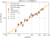 |
Fig. A.1. Mass-amplitude relation obtained using different modelling of the truncation radius; orange, green, and blue refer to the cases with rt = 4, rt = 2, and rt = 1, respectively. The red data points show the results for our reference model with rt = 3. We slightly displace the data points along the x-direction, computed with different truncation radius definitions, to make the results more visible. The orange lines exhibit the best-fit results for our reference case for the ∼1h case dataset, as in the first line of Table 2. |
Scaling relation parameters of the mass-amplitude relation.
Appendix B: Model systematics: 2h term
In this section we investigate how different model assumptions might also affect the recovered total matter density parameter. In Fig. B.1 we exhibit the combined posterior distributions, in redshift, of ΩM obtained assuming different values of the truncation radius. We find a degeneracy between the effects of ΩM and the truncation radius, with a small value of the truncation radius being compensated by an increase in the total matter density parameter. Specifically, we find a systematic deviation of the total matter density parameter of the order of 5.6%, 2.1%, and −2.5% for rt = 1, 2, and 4 with respect to our reference case rt = 3, respectively. In the same figure we also show the result obtained from the stacked profiles estimated without accounting for the signal around random centres. In this case there is an underestimate ΩM of approximately 13%.
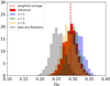 |
Fig. B.1. Combined posteriors, in redshift, for the recovered total matter density parameter assuming different values of the truncation radius. The red-filled histogram shows the posterior of our reference model with rt = 3. The gold, green, and blue histograms show the distributions of ΩM assuming rt = 4, 2, and 1, respectively. The grey histogram shows the result obtained from the stacked profiles estimated without accounting for the signal around random centres. The vertical red dashed line indicates the weighted average of the reference posterior distribution. |
In Fig. B.2 we show the posterior distribution of the total matter density parameter assuming a linear power spectrum for the 2h term adopting WMAP9 (Bennett et al. 2013) cosmological parameters with h = 0.7. The blue-filled histogram shows the results combing all redshifts together, while the red, orange, and green histograms display the results for the low, intermediate, and high redshift samples, respectively. We note full consistence in our posterior distributions, particularly when adopting a Planck18 or a WMAP9 cosmological parameters (and fixing h = 0.7) for the linear power spectrum when recovering ΩM. Using WMAP9 we slightly underestimate (by 2%) the total matter density parameter with respect to our reference case based on Planck18.
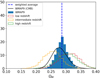 |
Fig. B.2. Posterior distributions of the total matter density parameter ΩM. The red, orange and green histograms show the results for the low, intermediate, and high redshift cluster samples, respectively. The blue histogram shows the posterior distribution combining all redshifts together; the dashed blue line indicates the median of the distribution. The black curve displays the posterior distribution obtained from the analysis of the CMB data by Bennett et al. (2013). |
Considering that the normalisation of the two-halo model depends on the halo bias parameter, we expect our results to also be dependent on the assumed bias model. Figure B.3 shows the impact of different bias model assumptions on the ΩM posterior distributions. Assuming the Sheth & Tormen (1999) and Sheth et al. (2001) biasing models we obtain a weighted average of the combined posteriors for ΩM that is respectively 3.5% and −3.2% different to the value obtained with our reference model, based on the Tinker et al. (2010) halo bias recipe.
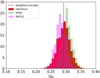 |
Fig. B.3. Combined posterior distributions obtained for different halo bias model. The red, green and magenta histograms show the cases obtained with the halo biases respectively from Tinker et al. (2010) (our reference case), Sheth & Tormen (1999), and Sheth et al. (2001). |
The deviations observed when changing the cosmology, the bias model, and the truncation radius are all comparable, but smaller than the statistical error of our measurement. These values place some perspective on the systematics requirements for future data.
All Tables
Constraints on ΩM obtained from the stacked weak lensing analyses at the three redshift ranges considered, and the combined redshifts.
All Figures
|
Fig. 1. Distribution of cluster centres in angular coordinates of the 6962 detections by AMICO divided into the KiDS-N (left) and KiDS-S (right) areas. Systems with 0.1 ≤ z ≤ 0.6 and with S/N > 3.5 are displayed. |
| In the text | |
|
Fig. 2. Differencial surface density profile model as a function of radius. Upper panel: model of the projected excess of surface mass density as a function of the comoving radial distance from the centre for a cluster with M200 = 1014 M⊙ h−1, c200 = 3 at redshift z = 0.3, with σoff = 0.3 and foff = 0.3. The radius enclosing 200 times the critical density corresponds to R200 = 1.47 Mpc h−1. The four one-halo and two-halo terms are shown with different colours and styles, as labelled. Second panel: relative differences, with respect to the reference, of the models with rt = 1, 2, and 4. Third panel: relative differences, with respect to the reference, of the models with the linear power spectrum estimated assuming different cosmological model parameters, as labelled. Shown for comparison (yellow dotted curve) is the relative difference between the prediction adopting WMAP9 cosmology and WMAP9, but fixing ΩM = 0.3 and h = 0.7. Bottom panel: relative differences, with respect to the reference, of two models constructed with either the Sheth & Tormen (1999) or the Sheth et al. (2001) biasing model. |
| In the text | |
|
Fig. 3. Excess of surface mass density profile around random centres for the three redshift bins into which the AMICO clusters have been divided: low (0.1 ≤ z < 0.3), intermediate (0.3 ≤ z < 0.45), and high (0.45 ≤ z ≤ 0.6) redshift. We created 10 000 realisations of the sample using random centres. The blue crosses, red diamonds, and green triangles show the average measurements in the three redshift intervals, extending the profiles up to 35 Mpc h−1 as in the 1h + 2h case. The black line displays the average over all redshifts. The error bars show square root of the diagonal terms of the corresponding covariances CRandoms(r, r′). The vertical pink area on the left gives the data points below 0.2 Mpc h−1, which we do not consider in our analysis. |
| In the text | |
|
Fig. 4. Example of covariances and differencial surface density profiles. Left panel: normalised covariance of the dataset corresponding to the bin with 0.1 ≤ z < 0.3 and 2.05 ≤ A < 2.75, stacking 96 detected clusters, computed with 10 000 bootstrap realisations of the stacked profile. Central panel: normalised covariance of the 10 000 realisations of the whole AMICO sample, randomly distributed in the survey footprints. Right panel: stacked excess surface mass density profile of the 1h case (blue crosses) and 1h + 2h case (orange circles). In both cases we subtract to the data points the stacked profiles around random centre. The error bars refer to the square root of the diagonal elements of the final covariance (Eq. (17)). The red arrows indicate the variation of the stacked profile when, for the corresponding redshift bin, the random contributions are subtracted from the data. The blue crosses and orange filled circles refer to two different binning schemes, giving the possibility to constrain the cluster-halo structural properties and the large-scale matter density distribution in which the clusters are located, respectively. |
| In the text | |
|
Fig. 5. Stacked excess surface mass density profiles of the clusters divided in different amplitude bins (from left to right) and redshift bins (from top to bottom). The blue and orange data points refer to the ∼1h and 1h + 2h cases, respectively. The corresponding error bars represent the square root of the diagonal terms in the corresponding covariance matrix. The blue and red solid curves show the best-fit models, which are the median values of the posterior distributions assessed with the MCMC, corresponding to the ∼1h and 1h + 2h cases, respectively. The blue and red curves are respectively dotted and dashed outside the corresponding dataset, especially the blue line below 0.2 and above 3.16 Mpc h−1, and the red line only below 0.2 Mpc h−1. The green curves show the two-halo term contribution. |
| In the text | |
|
Fig. 6. Mass-amplitude relation obtained in the ∼1h case, accounting for the full covariance in each amplitude and redshift interval. We compare our results (red data points) with those by Bellagamba et al. (2019) (black data points). The error bars show the 18th and 82nd percentiles of the posterior distributions. The blue solid line shows the scaling relation recovered by Bellagamba et al. (2019); the orange solid line exhibits our best-fit result. |
| In the text | |
|
Fig. 7. Posterior distributions of the parameters of the mass-amplitude relation in Eq. (18). The contours show the 68th and 95th percentiles of the distributions. For comparison, also shown are the results for α, β, and γ obtained by Bellagamba et al. (2019) (green squares) and when assuming a flat WMAP9 cosmology, fixing ΩM = 0.3 and h = 0.7. |
| In the text | |
|
Fig. 8. Concentration-mass relation obtained from our stacked weak lensing analysis of the AMICO-KiDS-DR3 clusters. Data points and error bars show the median and the 18th−82th percentiles of the posteriors distributions. Blue, orange and green colours refer to the low, intermediate and high redshift cluster sub-samples. The solid curves represent the predictions by Zhao et al. (2009) in three redshift intervals. For each data point, the numbers show the results for the c − M relation obtained adopting the truncation radius rt equal to 1, 2 and 4 – in unit of R200, respectively. The grey and light-grey shaded regions indicate 1 and 2-σln c = 0.25 scatter as measured in numerical simulations (Dolag et al. 2004; Giocoli et al. 2012a). The magenta line show the linear regression in the c − m relation computed using our reference results as dataset, while the shaded light-magenta region encloses the 1-σ uncertainties in both the slope and the intercept of the relation. In this case, we use the ODR routine in python considering the uncertainties in both mass and concentration. Dashed gold and dash-dotted cyan display the results by Sereno et al. (2017) – based on observational data – and Meneghetti et al. (2014) – on hydrodynamical simulations, respectively. |
| In the text | |
|
Fig. 9. Correlation between the recovered cluster mass and total matter density parameter from our stacked weak lensing analysis. The different coloured data points refer to three redshift ranges considered (see legend, top left corner). The blue solid line displays the weighted average of the various estimated ΩM for the different amplitude and redshift bins; the cyan shaded region encloses the 1σ uncertainty. The dashed red line gives the weighted average of the posterior distributions, as in Fig. 10. |
| In the text | |
|
Fig. 10. Posterior distributions of the total matter density parameter ΩM. The blue, orange, and green histograms show the results for the low, intermediate, and high redshift cluster samples, respectively. The red-filled histogram exhibits the posterior distribution combining all redshifts together; the dashed red line indicates the median of the distribution. The black curve displays the posterior distribution obtained from the analysis of the CMB data by Planck Collaboration VI (2020). |
| In the text | |
|
Fig. A.1. Mass-amplitude relation obtained using different modelling of the truncation radius; orange, green, and blue refer to the cases with rt = 4, rt = 2, and rt = 1, respectively. The red data points show the results for our reference model with rt = 3. We slightly displace the data points along the x-direction, computed with different truncation radius definitions, to make the results more visible. The orange lines exhibit the best-fit results for our reference case for the ∼1h case dataset, as in the first line of Table 2. |
| In the text | |
|
Fig. B.1. Combined posteriors, in redshift, for the recovered total matter density parameter assuming different values of the truncation radius. The red-filled histogram shows the posterior of our reference model with rt = 3. The gold, green, and blue histograms show the distributions of ΩM assuming rt = 4, 2, and 1, respectively. The grey histogram shows the result obtained from the stacked profiles estimated without accounting for the signal around random centres. The vertical red dashed line indicates the weighted average of the reference posterior distribution. |
| In the text | |
|
Fig. B.2. Posterior distributions of the total matter density parameter ΩM. The red, orange and green histograms show the results for the low, intermediate, and high redshift cluster samples, respectively. The blue histogram shows the posterior distribution combining all redshifts together; the dashed blue line indicates the median of the distribution. The black curve displays the posterior distribution obtained from the analysis of the CMB data by Bennett et al. (2013). |
| In the text | |
|
Fig. B.3. Combined posterior distributions obtained for different halo bias model. The red, green and magenta histograms show the cases obtained with the halo biases respectively from Tinker et al. (2010) (our reference case), Sheth & Tormen (1999), and Sheth et al. (2001). |
| In the text | |
Current usage metrics show cumulative count of Article Views (full-text article views including HTML views, PDF and ePub downloads, according to the available data) and Abstracts Views on Vision4Press platform.
Data correspond to usage on the plateform after 2015. The current usage metrics is available 48-96 hours after online publication and is updated daily on week days.
Initial download of the metrics may take a while.