| Issue |
A&A
Volume 649, May 2021
|
|
|---|---|---|
| Article Number | A89 | |
| Number of page(s) | 37 | |
| Section | Numerical methods and codes | |
| DOI | https://doi.org/10.1051/0004-6361/202039913 | |
| Published online | 21 May 2021 | |
Multiscale, multiwavelength extraction of sources and filaments using separation of the structural components: getsf
AIM, IRFU, CEA, CNRS, Université Paris-Saclay, Université Paris Diderot, Sorbonne Paris Cité, 91191 Gif-sur-Yvette, France
e-mail: This email address is being protected from spambots. You need JavaScript enabled to view it.
Received:
14
November
2020
Accepted:
22
February
2021
Abstract
High-quality astronomical images delivered by modern ground-based and space observatories demand adequate, reliable software for their analysis and accurate extraction of sources, filaments, and other structures, containing massive amounts of detailed information about the complex physical processes in space. The multiwavelength observations with highly variable angular resolutions across wavebands require extraction tools that preserve and use the invaluable high-resolution information. Complex fluctuating backgrounds and filamentary structures appear differently on various scales, calling for multiscale approaches for complete and reliable extraction of sources and filaments. The availability of many extraction tools with varying qualities highlights the need to use standard model benchmarks for choosing the most reliable and accurate method for astrophysical research. This paper presents getsf, a new method for extracting sources and filaments in astronomical images using separation of their structural components, designed to handle multiwavelength sets of images and very complex filamentary backgrounds. The method spatially decomposes the original images and separates the structural components of sources and filaments from each other and from their backgrounds, flattening their resulting images. It spatially decomposes the flattened components, combines them over wavelengths, detects the positions of sources and skeletons of filaments, and measures the detected sources and filaments, creating the output catalogs and images. The fully automated method has a single user-defined parameter (per image), the maximum size of the structures of interest to be extracted, that must be specified by users. This paper presents a realistic multiwavelength set of simulated benchmark images that can serve as the standard benchmark problem to evaluate qualities of source- and filament-extraction methods. This paper describes hires, an improved algorithm for the derivation of high-resolution surface densities from multiwavelength far-infrared Herschel images. The algorithm allows creating the surface densities with angular resolutions that reach 5.6″ when the 70 μm image is used. If the shortest-wavelength image is too noisy or cannot be used for other reasons, slightly lower resolutions of 6.8−11.3″ are available from the 100 or 160 μm images. These high resolutions are useful for detailed studies of the structural diversity in molecular clouds. The codes getsf and hires are illustrated by their applications to a variety of images obtained with ground-based and space telescopes from the X-ray domain to the millimeter wavelengths.
Key words: stars: formation / infrared: ISM / submillimeter: ISM / methods: data analysis / techniques: image processing / techniques: photometric
© A. Men’shchikov 2021
 Open Access article, published by EDP Sciences, under the terms of the Creative Commons Attribution License (https://creativecommons.org/licenses/by/4.0), which permits unrestricted use, distribution, and reproduction in any medium, provided the original work is properly cited.
1. Introduction
Multiwavelength far-infrared and submillimeter dust continuum observations with the large space telescopes Spitzer, Herschel, and Planck in the past decades greatly increased the amount and improved the quality of the available data in various areas of astrophysical research. Observed images with diffraction-limited angular resolutions and high sensitivity reveal an impressive diversity of the enormously complex structures, covering orders of magnitude in intensities and spatial scales. The images feature foremost the bright fluctuating backgrounds, omnipresent filaments, and huge numbers of sources of different physical nature, all blended with each other, whose appearance and resolution are often markedly different at short and long wavelengths. The massive amount of information that is coded in the fine structure of the observed images must contain clues to the complex physical processes taking place in space, but these clues are extremely difficult to decipher. It is quite clear that the era of these high-quality data from space telescopes and large ground-based interferometers, such as the Atacama Large Millimeter/submillimeter Array (ALMA), requires more sophisticated tools for their accurate analysis and correct interpretation than those developed for the lower-quality images of the past. Adequate extraction methods must be explicitly designed for the multiwavelength imaging observations with highly dissimilar angular resolutions across wavebands. They must also be able to handle the bright filamentary backgrounds that vary on all spatial scales, whose fluctuation levels differ by several orders of magnitude across the observed images.
The source- and filament-extraction methods are growing in numbers. In the area of star formation, a new method was published every year or two within the seven-year period after the launch of Herschel. Rosolowsky et al. (2008) devised dendrograms to describe the hierarchical structure of clumps observed in the data cubes from molecular line observations. The method carries out topological analysis of image structures by isophotal contours at varying intensity levels and represents them graphically as a tree. Molinari et al. (2011) created cutex to extract sources in star-forming regions observed with Herschel. The method analyzes multidirectional second derivatives of the observed image to detect sources, and it measures them by fitting elliptical Gaussians on a planar background to their peaks. Men’shchikov et al. (2012) developed getsources, the multiwavelength source extraction method for the Herschel observations of star-forming regions. The method spatially decomposes images, combines them into wavelength-independent detection images, subtracts the backgrounds of detected sources, and measures the sources, deblending them when they overlap. Kirk et al. (2013) presented csar for the Herschel images. The method analyzes areas of connected pixels that are bound by closed isophotal contours, descending to a predefined background level and partitioning peaks at their lowest isolated contours into sources. Berry (2015) created fellwalker to identify clumps in submillimeter data cubes. The method finds image peaks by tracing the line of the steepest ascent and identifies sources as the hill with the highest value found for all pixels in its neighborhood. Sousbie (2011) produced disperse to identify structures in the large-scale distribution of matter in the Universe. The method applies the computational topology to trace filaments and other structures. Men’shchikov (2013) developed getfilaments to improve the source extraction with getsources on the filamentary backgrounds observed with Herschel. The method separates filaments from sources in spatially decomposed images and subtracts them from the detection images, thereby reducing the rate of spurious sources. Schisano et al. (2014) devised a Hessian matrix-based approach to extract filaments in Herschel observations of the Galactic plane. The method analyzes multidimensional second derivatives to identify filaments and determine their properties. Clark et al. (2014) presented rht to characterize fibers in the interstellar H I medium. The method has been applied to various observations of diffuse H I, revealing alignment of the fibers along magnetic fields. Koch & Rosolowsky (2015) published filfinder to identify filaments in the Herschel images of star-forming regions. the method applies a mathematical morphology approach to isolating filaments in observed images. Juvela (2016) presented tm to trace filaments in observed images. The method matches a predefined template (stencil) of an elongated structure at each pixel of an image by shifting and rotating the template and analyzing the parameters of the matches.
These extraction methods all have several important issues. Sources and filaments are handled completely independently by these methods, although numerous Herschel observations have demonstrated that there is a tight physical relation between them. Most sources are found in filamentary structures, and the corresponding starless, prestellar, and protostellar cores are thought to form inside the structures that are created by dynamical processes, magnetic fields, and gravity within a molecular cloud. All major structural components of the observed images, that is, the background cloud, filamentary structures, and sources, are heavily blended with each other; curved filaments are even blended with themselves. The degree of their blending increases at longer wavelengths with lower angular resolutions, which increases the inaccuracies in their detections, measurements, and interpretations.
Most of the extraction methods focus on detecting structures, whereas the most important and difficult problem is measuring them accurately. Numerous algorithms only partition the image between sources and do not allow them to overlap, although deblending of the mixed emission of the structural components is an indispensable property of an accurate extraction method. For best detection and measurement results, source-extraction methods must be able to separate underlying filamentary structures and filament-extraction methods must be able to separate sources. The existing source- and filament-extraction methods use completely different approaches, and the quality of their results is expected to be very dissimilar.
It seems unlikely that methods that are based on very different approaches would give consistent results in terms of detection completeness, number of false-positive detections, and measurement accuracy. In practice, various methods do perform very differently, as can be shown quantitatively on simulated benchmarks for which the properties of all components are known. This highlights the need of systematic comparisons of different methods in order to understand their qualities, inaccuracies, and biases. The danger is real that numerous uncalibrated methods are applied for the same type of star formation studies, which would give inconsistent, contradictory results and incorrect conclusions. This would create serious, lasting problems for the science.
Source- and filament-extraction methods are the critically important tools that must be calibrated and validated using a standard set of benchmark images with fully known properties of all components before they are applied in astrophysical contexts. It would be desirable to use the same extraction tool to exclude any biases or dissimilarities that are caused by different methods. If a new extraction method is to be used, it must be tested on standard benchmarks to ensure that its detection and measurement qualities are consistent or better. This approach is usually practiced within research consortia, but this does not solve the global problem that the results obtained from the same data by different consortia or research groups using different tools may still be affected by the uncalibrated (or suboptimal) tools that were used.
This paper presents getsf, a new multiwavelength method for extracting sources and filaments. It also describes a realistic simulated benchmark, resembling the Herschel images of star-forming regions, which is used below to illustrate the method and in a separate paper (Men’shchikov 2021) to quantitatively evaluate its performance. The multiwavelength benchmark simulates the images of a dense cloud with strong nonuniform fluctuations, a wide dense filament with a power-law intensity profile, and hundreds of radiative transfer models of starless and protostellar cores with wide ranges of sizes, masses, and profiles. The simulated benchmark with fully known parameters allows quantitative analyses of extraction results and conclusive comparisons of different methods by evaluating their extraction completeness, reliability, and goodness, along with the detection and measurement accuracies. The multiwavelength images can serve as the standard benchmark problem for other source- and filament-extraction methods, allowing researchers to perform their own tests and choose the most reliable and accurate extraction method for their studies. Instead of publishing benchmarking results for some of the existing methods, it seems a better idea to provide researchers with the benchmark1 and a quality evaluation system (Men’shchikov 2021) to enable comparisons of the methods of their choice. In practice, this approach of having own experience is much more convincing and it allows a consistent evaluation of newly developed methods.
The new source and filament extraction method getsf represents a major improvement over the previous algorithms getsources, getfilaments, and getimages (Men’shchikov et al. 2012; Men’shchikov 2013, 2017, hereafter referred to as Papers I, II, and III); throughout this paper, the three predecessors are collectively referred to as getold. The new method (Fig. 1) consistently handles two types of structures, sources and filaments, that are important for studies of star formation, separating the structural components from each other and from their backgrounds. All major processing steps of getsf employ spatial decomposition of images into a number of finely spaced single-scale images to better isolate the contributions of structures with various widths. The method produces accurately flattened detection images with uniform levels of the residual background and noise fluctuations. To detect sources and filaments, getsf combines independent information contained in the multiwaveband single-scale images of the structural components, preserving the higher angular resolutions. Then getsf measures and catalogs the detected sources and filaments in their background-subtracted images. The fully automated method needs only one user-defined parameter, the maximum size of the structures of interest to extract, constrained by users from the input images on the basis of their research interests.
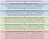 |
Fig. 1. Flowchart of the image processing steps in getsf. The colored blocks represent preparation (purple), background subtraction (blue), image flattening (green), and extraction of sources and filaments (red). |
This work follows Papers I–III in advocating a clear distinction between the words source and object, unlike many publications in which it is implicitly assumed that the two are completely equivalent. “Source” is used in the context of the source extractions and statistical analysis of their results, and “object” is only used in the context of the physical interpretation of the extracted sources. In this paper, the sources are defined as the emission peaks (mostly unresolved) that are significantly stronger than the local surrounding fluctuations, indicating the presence of the physical objects in space that produced the observed emission. The implicit assumption that an unresolved far-infrared source on a complex fluctuating background contains emission of just one single object is invalid in general. Too often, an emission peak is actually a blend of many components, produced by different physical entities. This is illustrated by the recent images of the massive star-forming cloud W43-MM1 (Motte et al. 2018), obtained with the ALMA interferometer. This object appears as a single source in the Herschel images, even with the 5.6 and 11.3″ resolutions at 70 and 160 μm. However, the ALMA image (Sect. 4.8) displays a rich cluster of much smaller sources that are unresolved or just slightly resolved even at the 0.44″ resolution.
Section 2 describes the new multiwavelength benchmark for source- and filament-extraction methods, resembling the Herschel observations of star-forming regions. Section 3 presents getsf, the new source- and filament-extraction method, employing separation of the structural components. Section 4 illustrates the performance of getsf on a large variety of images that were obtained with different telescopes in a wide spectral range, from X-rays to millimeter wavelengths. Section 5 describes all strengths and limitations of getsf. Section 6 presents a summary of this work. Appendix A discusses inaccuracies of the surface densities and temperatures, derived by spectral fitting of the images. Appendix B describes the single-scale spatial decomposition that is used by getsf in its processing steps. Appendix C gives details on the software.
In this paper, images are represented by capital calligraphic characters (e.g., 𝒜, ℬ, 𝒞) and software names and numerical methods are typeset slanted (e.g., getsf) to distinguish them from other emphasized words. The curly brackets are used to collectively refer to either of the characters, separated by vertical lines. For example, {a|b} refers to a or b and {A|B}{a|b}c expands to A{a|b}c or B{a|b}c, as well as to Aac, Abc, Bac, or Bbc.
2. Benchmark for source and filament extractions
Realistic multiwavelength, multicomponent images of a simulated star-forming region were computed to present getsf in this paper and to compare its performance with the previous benchmark that was used in Papers I and III. The benchmark images were created for all Herschel wavebands (at λ of 70, 100, 160, 250, 350, and 500 μm). They consist of independent structural components: a background cloud ℬλ, a long filament ℱλ, round sources 𝒮λ, and small-scale instrumental noise 𝒩λ:
 (1)
(1)
where 𝒞λ = ℬλ + ℱλ is the emission intensity of the filamentary background. All simulated images were computed on a 2″ pixel grid with 2690 × 2690 pixels, covering 1.5° ×1.5° or 3.7 pc at a distance D = 140 pc of the nearest star-forming regions (e.g., those in Taurus or Ophiuchus).
2.1. Simulated filamentary background
An image of the background surface density was computed from a purely synthetic scale-free background 𝒟A (cf. Paper I), with NH2 ∼ 2.7 × 10²⁰ to 5 × 1022 cm−2 that had uniform fluctuations across the entire image. To simulate complex astrophysical backgrounds with strongly nonuniform fluctuations (e.g., Könyves et al. 2015), 𝒟A was multiplied by a circular shape 𝒫 with a radial profile defined by Eq. (2) below (with Θ = 1500″ and ζ = 2), normalized to unity and centered on the image; finally, a constant value of 1.5 × 1021 cm−2 was added to increase the minimum value. The surface densities of the resulting background cloud image 𝒟B (Fig. 2) are 1.5 × 10²¹ to 4.8 × 1022 cm−2 and the fluctuations differ by approximately two orders of magnitude. The total mass of the cloud is MB = 1.78 × 10³ M⊙.
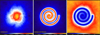 |
Fig. 2. Background surface densities (𝒟B, 𝒟C) and average line-of-sight dust temperatures (𝒯C) used to compute the simulated Herschel images 𝒞λ of the filamentary cloud from Eq. (4). Square-root color mapping. |
To simulate filamentary backgrounds, a long spiral filament was added to the background cloud 𝒟B. The spiral shape was chosen so that the filament occupied various areas of the cloud with very different surface densities and to cause the filament to be blended (with itself) to some extent. The spiral filament image 𝒟F has a crest value of N0 = 1023 cm−2, a full width at half-maximum (FWHM) W = 0.1 pc, and a radial profile similar to those observed with Herschel in star-forming regions (e.g., Arzoumanian et al. 2011, 2019),
 (2)
(2)
where θ is the angular distance, Θ is the structure half-width at half-maximum, and ζ is a power-law exponent. With Θ = 75″ (or 0.05 pc at D = 140 pc) and ζ = 1.5, this Moffat (Plummer) function approximates a Gaussian of 0.1 pc (FWHM) in its core and it transforms into a power-law profile NH2(θ) ∝ θ−3 for θ ≫ Θ. The filament mass MF = 3.04 × 10³ M⊙ and length LF = 10.5 pc correspond to the linear density ΛF = 290 M⊙ pc−1. The resulting surface densities 𝒟C = 𝒟B + 𝒟F of the filamentary cloud are in the range of 1.7 × 10²¹ to 1.4 × 1023 cm−2 (Fig. 2), and its total mass is MC = 4.82 × 10³ M⊙.
To approximate the nonuniform line-of-sight dust temperatures of the star-forming clouds observed with Herschel (e.g., Men’shchikov et al. 2010; Arzoumanian et al. 2019), an image of average line-of-sight temperatures was improvised as
 (3)
(3)
The pixel values of the resulting temperature image 𝒯C range between 15 K in the innermost areas of the filamentary cloud and 20 K in its outermost parts (Fig. 2). The temperatures from Eq. (3) were used to simulate the cloud images 𝒞λ in all Herschel wavebands, assuming optically thin dust emission:
 (4)
(4)
where Bν is the blackbody intensity, κν is the dust opacity, η = 0.01 is the dust-to-gas mass ratio, μ = 2.8 is the mean molecular weight per H2 molecule, and mH is the hydrogen mass. The dust opacity was parameterized as a power law κν = κ0(ν/ν0)β with κ0 = 9.31 cm2 g−1 (per gram of dust), λ0 = 300 μm, and β = 2.
2.2. Simulated starless and protostellar cores
To populate the filamentary cloud with realistic sources, 156 radiative transfer models were computed by a numerical solution of the dust continuum radiative transfer problem in spherical geometry (using modust, Bouwman 2001). The models adopted tabulated absorption opacities κabs for dust grains with thin ice mantles (Ossenkopf & Henning 1994), corresponding to a density nH = 106 cm−3 and coagulation time t = 105 yr. The opacity values at λ > 160 μm were replaced with a power law κλ ∝ λ−2, consistent with the parameterization used in Eq. (4).
The models of three populations of starless cores and one population of protostellar cores cover wide ranges of masses (from 0.05 to 2 M⊙) and half-maximum sizes (from ∼0.001 to 0.1 pc). Density profiles of the critical Bonnor–Ebert spheres were adopted for starless cores, whereas the protostellar cores have power-law densities ρ(r) ∝ r−2. Starless cores consist of low-, medium-, and high-density subpopulations, following the M ∝ R relation for the isothermal Bonnor–Ebert spheres (with TBE = 7, 14, 28 K) in the area of the mass–radius diagram occupied by prestellar cores observed in the Ophiuchus and Orion star-forming regions (Motte et al. 1998, 2001).
Both types of cores were embedded in background spherical clouds with a uniform surface density of 3 × 1021 cm−2 and outer radius of 1.4 × 10⁵ AU (1000″ or 0.68 pc). In an isotropic interstellar radiation field (Black 1994) with the strength parameter G0 = 10 (e.g., Parravano et al. 2003), the embedding clouds acquired temperatures of T ≈ 22 K at their edges, consistent with the highest values of 𝒯C from Eq. (3). The embedding clouds lowered T(r) toward the interiors of both starless and protostellar cores. Accreting protostars in the centers of the protostellar cores, however, produced luminosity LA ∝ M and thus sharply peaked temperature distributions deeper in their central parts.
2.3. Complete simulated images
Individual surface density images of the models of 828 starless and 91 protostellar cores were distributed in the dense areas (NH2 ≥ 5 × 1021 cm−2) of the filamentary cloud 𝒟C. They were added quasi-randomly, without overlapping, to the 𝒟C image at positions, where their peak surface density exceeded that of the cloud NH2 value. An initial mass function (IMF)-like power-law mass function with a slope dN/dM of −1.7 was used to determine the numbers of models per mass bin δ log10M ≈ 0.1 in each of the four populations. This resulted in the surface densities 𝒟S, the intensities 𝒮λ of sources (Fig. 3), and in the complete simulated images 𝒞λ + 𝒮λ.
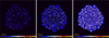 |
Fig. 3. Component of sources 𝒮λ that is composed of the images of radiative transfer models of 828 starless and 91 protostellar cores and convolved to the Herschel resolutions Oλ (cf. Sect. 1), shown at three selected wavelengths. Only the bright unresolved emission peaks of the protostellar cores, clearly visible at 100 μm, appear in the 70 μm image (not shown). Square-root color mapping. |
The final simulated Herschel images ℋλ from Eq. (1) of the modeled star-forming region were obtained by adding different realizations of the random Gaussian noise 𝒩λ at 70, 100, 160, 250, 350, and 500 μm and convolving the resulting images to the angular resolutions Oλ of 8.4, 9.4, 13.5, 18.2, 24.9, and 36.3″, respectively (Fig. 4). The resulting images ℋλ have σ noise levels of 6, 6, 5.5, 2.5, 1.2, and 0.5 MJy sr−1, resembling the actual noise measured in the Herschel images of the Rosette molecular complex (Motte et al. 2010).
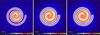 |
Fig. 4. Images ℋλ of the simulated star-forming region, defined by Eq. (1)), shown at three selected wavelengths. The benchmark images are a superposition of four structural components: the background ℬλ, the filament ℱλ, the sources 𝒮λ, and the noise 𝒩λ. Two simpler variants of this benchmark are also available: without the filament and without the background. Square-root color mapping. |
3. Source- and filament-extraction method
The main processing steps of getsf are outlined in Fig. 1, where several major blocks of the algorithm are highlighted. The method may be summarized as follows: (1) preparation of a complete set of images for an extraction, (2) separation of the structural components of sources and filaments from their backgrounds, (3) flattening of the residual noise and background fluctuations in the images of sources and filaments, (4) combination of the flattened components of sources and filaments over selected wavebands, (5) detection of sources and filaments in the combined images of the components, and (6) measurements of the properties of the detected sources and filaments.
Like its predecessors, getsf has just a single, user-definable parameter: the maximum size (width) of the structures of interest to extract. Internal parameters of getsf have been carefully calibrated and verified in numerous tests using large numbers of diverse images (both simulated and real-life observed images) to ensure that getsf works in all cases. This approach rests on the conviction that high-quality extraction methods for scientific applications must not depend on the human factor. It is the responsibility of the creator of a numerical method to make it as general as possible and to minimize the number of free parameters as much as possible. An internal multidimensional parameter space of complex numerical tools must never be delegated to the end user to explore if the aim is to obtain consistent and reliable scientific results.
3.1. Preparation of images for extraction
The multiwavelength extraction methods must be able to use all available information contained in the observed images across various wavebands with different angular resolutions. It is usually beneficial to collect all available images for a specific region of the sky under study.
3.1.1. Original observed set of images
To prepare multiwavelength ℋλ for processing with getsf, it is necessary to convert them into the images ℐλ, all on the same grid of pixels. To this end, getsf resamples all images (using swarp, Bertin et al. 2002) on a pixel size, chosen to be optimal for the highest-resolution images available. It is very important to carefully verify alignment of the resampled ℐλ and correct it (if necessary) to ensure that all unresolved intensity peaks remain on the same pixel across all wavebands. To reveal possible misalignments, it is sufficient to open each pair of prepared images in ds9 (Joye & Mandel 2003) and blink the two frames, going from the highest-resolution to the lowest-resolution images.
Most astronomical images have irregularly shaped coverage and limited usable areas that differ between wavebands. To include only the “good” parts of the ℐλ coverage in the image processing, it is necessary to create masks ℳλ (with pixel values 1 or 0). With these masks, getsf can process only the good areas of ℐλ that have a mask value of 1. To facilitate the image preparation, getsf always creates default masks ℳλ = 1. However, for most real observations, the masks must be prepared very carefully and independently for each image. To manually create the masks, one can use imagej (Abràmoff et al. 2004) or gimp2 that allows users to create a polygon over an image, convert the polygon into a mask, and save it in the FITS format.
3.1.2. Derived high-resolution images
The multiwavelength far-infrared Herschel images open the possibility of computing maps of surface density and dust temperature by fitting the spectral shapes Πλ of the image pixels. The standard procedure assumes that (1) the original images represent optically thin thermal emission of dust grains with a power-law opacity κλ ∝ λ−β and a constant β value, (2) the dust temperature is constant along the lines of sight passing through each pixel of the images, and (3) the lines of sight are not contaminated by unrelated radiation at either end, in front of the observed structures and behind them. Unfortunately, one or more of the assumptions are likely to be invalid, especially the stipulation of the opacity law and the constant line-of-sight temperatures (e.g., Men’shchikov 2016). The values of the derived surface densities and temperatures therefore must be considered as fairly unreliable and implying large error bars.
When we assume that the observations include the Herschel images, the spectral shapes Πλ of each pixel can be fit at several wavelengths (160−500 μm) and resolutions (18.2−36.3″), which results in three sets of surface densities and dust temperatures. The highest-resolution derived images are the least reliable because they are obtained from fitting only two images (at 160 and 250 μm), whereas the lowest-resolution maps are the most accurate because they come from fitting four independent images (at 160, 250, 350, and 500 μm).
In an attempt to combine the higher accuracy of the lower-resolution images with the higher angular resolutions of the less accurate images, Palmeirim et al. (2013) published a simple algorithm that uses complementary spatial information contained in the observed images to create a surface density image with the resolution OP = 18.2″ of the 250 μm image. When this approach is extended to temperatures, the sharper images can be computed by adding the higher-resolution information to the low-resolution images as differential terms,
 (5)
(5)
where the base surface density and temperature {𝒟|𝒯}4 are derived by fitting the 160, 250, 350, and 500 μm images at the lowest resolution O500 = 36.3″. The additional terms, containing the higher-resolution contributions, are produced by unsharp masking,
 (6)
(6)
where {𝒟|𝒯}3 are computed by fitting the three images at 160, 250, and 350 μm at the resolution O350 = 24.9″, and {𝒟|𝒯}2 are obtained by fitting the two images at 160 and 250 μm at the resolution O250 = 18.2″; the Gaussian kernels 𝒢{3|4} convolve the images to the next lower resolutions O{350|500}.
The following generalization of the above algorithm allows deriving surface densities and temperatures with any (arbitrarily high) angular resolution existing among the observed ℐλ. The three independently derived maps of temperatures 𝒯{2|3|4} with the resolutions of 18.2−36.3″ and six observed Herschel images with their native resolutions Oλ of 8.4−36.3″ define 18 surface densities,
 (7)
(7)
with the assumptions and parameterizations of Eq. (4). It is required that the resolution of temperatures must not be higher than Oλ, which excludes 𝒟O3502 and 𝒟O500{2|3} from the algorithm and provides 15 independently computed variants of the surface densities of the observed region, with different resolutions. The high-resolution surface density image is computed as
 (8)
(8)
where λH denotes the wavelength of the image ℐλH with the desired angular resolution OH ≡ OλH and the differential terms with higher-resolution information are obtained by the same unsharp masking,
 (9)
(9)
where 𝒢Oλ+ is the Gaussian kernel (regarded as the delta function at 500 μm), convolving 𝒟Oλ{2|3|4} to a lower resolution of the next longer wavelength. For images at λ < 250 μm, only the positive values of δ𝒟Oλ{2|3|4} are used in Eq. (8) to circumvent the problem of creating artificial depressions and negative pixels around strong peaks due to the resolution mismatch (Oλ < O250) between ℐλ and the lower-resolution 𝒯{2|3|4} in Eq. (7).
The problem is caused by the sharp radial temperature gradients toward the unresolved centers of protostellar cores (cf. Men’shchikov 2016). They are smeared out by the low resolutions of 18.2−36.3″, hence the fitting of Πλ leads to underestimated temperatures 𝒯{2|3|4} and overestimated values (within an order of magnitude) of peak surface densities at higher resolutions Oλ < O250. This means that unsharp masking of the overestimated peaks could create negative annuli in δ𝒟Oλ{2|3|4} and negative pixels in 𝒟OH. Fortunately, the surface densities are quite accurate outside the unresolved peaks (Appendix A).
A slight modification of Eq. (8) allows deriving the high-resolution surface densities with an enhanced contrast of all unresolved or slightly resolved structures,
 (10)
(10)
where the positive parts of the differential high-resolution terms from Eq. (9) are added to 𝒟OH. These high-contrast images may be useful for detection of unresolved structures because the latter are usually diluted by the observations with insufficient angular resolution; a higher contrast improves their visibility.
A high-resolution temperature 𝒯OH, consistent with the high-resolution surface density 𝒟OH, is computed by numerically inverting the Planck function,
 (11)
(11)
with  , where c is the speed of light. The high-resolution images {𝒟|𝒯}13″ are shown in Fig. 5 along with the true simulated 𝒟C + 𝒟S (Sect. 2.3). A comparison demonstrates that the pixel-fitting procedure reduces visibility of many unresolved or slightly resolved starless cores, which is the manifestation of the invalid assumption of the uniform line-of-sight temperatures. Starless (prestellar) cores have lower temperatures in their centers, and their smearing by an insufficient resolution leads to overestimated temperatures that suppress the surface density peaks (cf. Fig. A.1).
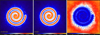 |
Fig. 5. Derived surface densities and temperatures (Sect. 3.1.2). The true model image 𝒟C + 𝒟S and the hires surface density 𝒟13″ and temperature 𝒯13″ derived from Eq. (8) with λH = 160 μm (OH = 13.5″) are shown. Many of the sources, clearly visible in the true image (left), are not discernible in the derived surface density (middle) because of the inaccuracies in the temperatures from fitting spectral shapes Πλ. Square-root color mapping, except the right panel with linear mapping. |
The new hires algorithm, outlined by Eqs. (7)–(11), brings the benefits of a resolution OH ≈ 8″, twice better than OP and four times better than O500, if the image quality at the shortest wavelengths permits this. Moreover, the angular resolutions of the Herschel images at 70, 100, and 160 μm, obtained with a slow scanning speed of 20″ s−1, are even higher: 6, 7, and 11″, respectively. These observations, illustrated in Fig. 6, allow deriving the surface densities and temperatures with OH ≈ 6″, a three times better resolution than when using Eq. (5). If the 70 μm image is too noisy or there is evidence of its strong contamination by emission unrelated to that of the adopted dust grains (e.g., polycyclic aromatic hydrocarbons or transiently heated very small dust grains), then the derived images may still have the 7−13″ resolution of the 100 or 160 μm wavebands. In addition to the high resolution, the images from Eq. (8) also have a better quality than those from Eq. (5) because they accumulate all available high-resolution information from the (up to 15) independently computed images 𝒟Oλ{2|3|4} that use all three temperatures 𝒯{2|3|4} with each original ℐλ.
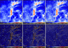 |
Fig. 6. High-resolution surface densities obtained for the Herschel images of Cygnus X (HOBYS project, Motte et al. 2010; Hennemann et al. 2012; Bontemps et al., in prep.). The top row shows the hires surface densities 𝒟OH from Eq. (8) with OH = 18.2″ and 5.9″ resolutions, and the high-contrast |

The hires algorithm works with any number 2 ≤ N ≤ 6 of Herschel wavebands. If the 160 μm image is unavailable or disabled, then the temperature 𝒯2 at the resolution O250 is removed from Eq. (7) and 𝒯{3|4} at the resolutions O{350|500} are obtained from fitting of only the 250, 350, and 500 μm images. If the 250 μm image is also unavailable or disabled, then only the single temperature 𝒯4 at the lowest resolution O500 remains in Eq. (7), obtained from the 350 and 500 μm images. Although the algorithm is unaffected by the changes, the reduction in the number of independently derived temperatures would lower the angular resolution and accuracy of the resulting surface density image. The improved algorithm can use the realistic, non-Gaussian point-spread functions (PSF) published by Aniano et al. (2011). However, the surface densities are largely determined by the SPIRE bands with nearly Gaussian PSFs, whereas only the PACS 160 μm band is used in the pixel fitting. The benchmark tests have shown that effects of the realistic PSFs on surface densities are very small, at percent levels, much smaller than the general uncertainties of the pixel-fitting methods (Appendix A). It is therefore sufficient to use the Gaussian PSFs when surface densities are derived.
For some studies, it might be useful to have all images at the same wavelength-independent angular resolution. With the high-resolution surface densities and temperatures from Eqs. (8) and (11), it is straightforward to obtain such images:
 (12)
(12)
with the assumptions and parameterizations of Eq. (4). For example, the intensities 𝒥λ13″ at 250, 350, and 500 μm would be sharper than ℐλ by the factors 1.3, 1.8, and 2.7, respectively.
When the available original set of images ℐλ allows creation of 𝒟OH, it is advantageous to have it complement the original data set, handling it as an image ℐƛ “observed” in a fictitious waveband ƛ. In the multiwavelength extractions with getsf, it may be recommended to use 𝒟OH for better detections and deblending of dense structures. The surface densities are not accurate enough for source measurements, as demonstrated in Appendix A and Men’shchikov (2016).
The following presentation and discussion of getsf implicitly assumes that the additional detection images are contained in the set of images ℐλ. In other words, all supplementary wavebands are included in the set of λ prepared for extraction. The latter was done for a multiwavelength data set that included all images in the Herschel wavebands (Fig. 4) and the high-resolution surface density ℐƛ ≡ 𝒟13″ (Fig. 5), a total of NW = 7 wavelengths.
3.1.3. Practical definition of maximum size
Before starting any extraction with getsf, it is necessary to formulate the aim of the study and determine what structures of interest are to be extracted. The method knows and is able to separate three types of structures: sources, filaments, and backgrounds. To separate the structural components with getsf, the maximum size {X|Y}λ of the sources (Xλ) and filaments (Yλ) of interest needs to be manually (visually) estimated from the prepared ℐλ independently for each waveband, which can be accomplished by opening an image in ds9 and placing a circular region fully covering the width of the largest structure. The maximum size of structures is the single physical parameter that the method needs to know for each observed image. Being a function of the type of structures (sources, filaments) and the waveband λ, it is split into Xλ and Yλ in this paper for convenience.
The maximum size {X|Y}λ is defined as the footprint radius (in arcsec) of the largest source and the widest filament to be extracted. A footprint size has the meaning of a full width at zero (background) level: the largest two-sided extent from a source peak or filament crest at which this structure is still visible in ℐλ against its background. For a Gaussian intensity distribution, the footprint radius is slightly larger than the half-maximum width Hλ of a structure. For a power-law intensity profile, the footprint radius may become much larger than Hλ. If the widest filaments of interest are blended (overlapping each other with their footprints), Yλ must be increased accordingly to approximate the full extent of the blend. In contrast, it is not necessary to adjust Xλ for blended sources because their final background will be determined from their footprints at the measurement step (Sect. 3.4.6).
It is not necessary (also not possible) to evaluate the maximum size parameter {X|Y}λ very precisely, a 50% accuracy is quite sufficient. Its purpose is to set a reasonable limit to the spatial scales when separating the structural components, and to the size of the structures to be measured and cataloged. The method works with spatially decomposed images, and it needs to know the maximum scale. It makes no sense to perform the decomposition up to a very large scale if the extraction is aimed at much smaller sources or narrower filaments. The method has no limitations with respect to the sizes (widths) of the structures to extract. However, it is important to avoid detecting, measuring, and cataloging the peaks that are unnecessarily too wide because they would likely overlap with other sources of interest, which potentially would make their measurements less accurate.
To extract all structures in the benchmark images presented in Sect. 2, the estimated Xλ values for sources are 16, 25, 30, 150, 150, and 150″, whereas the estimated Yλ values for the filament are 350″ in all six Herschel wavebands (Fig. 4); in the additional surface density image ℐƛ ≡ 𝒟13″ (Fig. 5), the {X|Y}ƛ values are the same as those for the 250−500 μm images.
3.2. Backgrounds of the structural components
Complex observed images may be radically simplified by subtracting backgrounds on spatial scales much larger than the maximum size {X|Y}λ. The independent largest sizes for sources and filaments effectively define two different backgrounds for the two scales. The Xλ-scale background ℬλX is derived to separate the component of sources 𝒮λ, whereas the Yλ-scale background ℬλY is obtained to separate the component of filaments ℱλ. The backgrounds are collectively referred to as ℬλ{X|Y}.
The true background under the observed structures is fundamentally unknown, and it is a major source of large uncertainties and measurement inaccuracies, especially for the faintest structures. In practice, the backgrounds ℬλ{X|Y} are defined in getsf as the smooth intensity distributions on spatial scales Sj larger than 4{X|Y}λ that remain in ℐλ after a complete removal of all sources or filaments with the maximum size of {X|Y}λ. In contrast to the background derivation by median filtering (getimages, Paper III), which may become extremely slow for very large images and wide structures, getsf employs a more direct, precise, and effective clipping algorithm to separate the structures.
3.2.1. Decomposition of the original images
In general, observed images are very complex blends of various structural components on different spatial scales, and great advantages are obtained when a spatial decomposition is used to simplify the images (cf. Papers I and II). Following the getold approach, getsf employs successive unsharp masking (Appendix B) to decompose the original images ℐλ into a set of single-scale images ℐλj (Fig. 7). It also uses an iterative algorithm (Appendix B) to determine a single-scale standard deviation σλj, as well as its total value σλ, which are used to separate the structural components present in ℐλ.
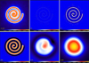 |
Fig. 7. Spatial decomposition (Sect. 3.2.1, Appendix B) for ℐƛ ≡ 𝒟13″ from Eq. (8) in single scales between 4 and 1400″. The original hires surface density (top left) and decomposed ℐƛj on selected scales Sj that differ by a factor of 4 are plotted. The remaining largest scales 𝒢NS∗ℐƛ (bottom right) are outside the decomposition range. Linear color mapping. |
3.2.2. Separation of the structural components
The backgrounds ℬλ{X|Y} are computed by cutting small round peaks and elongated structures off the decomposed images ℐλj and recovering the full images using Eq. (B.4). It is important to note that the appearance of the structures in the decomposed images depends on both the spatial scale and intensity level.
To remove the structural components, getsf slices ℐλj by a number NL of intensity levels Iλjl, spaced by δlnIλj = 0.05 from the image maximum down to σλj for sources and to 0.3σλj for filaments. Each slice l cuts through all the structures present in ℐλj on that intensity level, producing various shapes of connected pixels,
 (13)
(13)
Relatively round source-like peaks in ℐλj may be effectively distinguished from elongated structures by the number of connected pixels Nλjl that their shapes occupy in the slice ℐλjl (cf. Papers I and II). The single-scale images indeed most clearly show the structures with matching sizes (Hλ ≈ Sj), whereas the signals from much narrower and much wider structures are suppressed. As a consequence, the source-like shapes occupy relatively small areas of connected pixels in ℐλjl that are comparable to the area  of the convolution kernel 𝒢j. In contrast to the round peaks, elongated shapes in ℐλjl have greater lengths Lλ than widths Wλ ≈ Sj, which means that the filamentary shapes in slices ℐλjl extend over much larger areas than
  .
.
In addition to Nλjl, getsf uses two more quantities to discriminate between sources and filaments: elongation Eλjl and sparsity Sλjl. They are defined by the major and minor sizes (aλjl and bλjl) of each cluster of connected pixels, obtained from intensity moments (cf. Appendix F in Paper I),
 (14)
(14)
where Δ is the pixel size. Only simple and relatively straight filamentary shapes can be identified in ℐλjl by their elongation. Most of the actually observed filaments in space are shaped quite irregularly on different scales and intensity levels. The elongation Eλjl alone cannot be used to quantify strongly curved, not very dense clusters of connected pixels that meander around (e.g., a spiral structure). Although Eλjl may well be close to unity for sparse shapes, high values of Sλjl for these structures would indicate that they do not belong to sources.
The structural components are separated in single scales ℐλj using the three quantities described above. The shapes produced by sources in a slice ℐλjl are not very elongated, not very sparse, and not very large. In contrast, the shapes produced by filaments in a slice ℐλjl are elongated or sparse. Hence, these definitions for the source-like and filament-like shapes are written as
 (15)
(15)
where the limiting values of elongation and sparsity were determined empirically from numerous benchmark extractions. The ξλj factor accounts for the fact that the area of a decomposed unresolved peak increases nonlinearly toward the smallest spatial scales Sj ≲ Oλ. The factor may be determined empirically by decomposing an unresolved peak 𝒫 in single scales 𝒫j (Fig. B.1) and finding the distances θ, where the one-dimensional profile Pj(θ) through the peak has dPj/dθ = 0 for Pj < 0,
 (16)
(16)
The ξλj factor ensures that Nλjl has appropriate values and that single-scale peaks are clipped cleanly on all spatial scales.
Various shapes formed by connected pixels are identified and analyzed in each single-scale slice using the tintfill algorithm (Smith 1979)3, previously employed by getold to detect sources and filaments (Papers I and II). Deriving the background ℬλX of sources, getsf decomposes ℐλ and removes all source-like shapes from ℐλjl, according to their definition in Eq. (15), in an iterative procedure (Sect. 3.2.3). Deriving the background ℬλY of filaments, getsf decomposes ℬλX and removes all filament-like shapes from ℬλXjl, according to their definitions in Eq. (15), in the same iterative procedure. The shapes are erased from each slice l by setting all their pixels to zero.
3.2.3. Reconstruction of the backgrounds
When we denote with ℬλ{X|Y}jlC either of the single-scale background slices ℬλXjlC or ℬλYjlC after the shape removal, the backgrounds on scale j are reassembled from the clipped slices as
 (17)
(17)
To properly reconstruct the complete backgrounds ℬλ{X|Y} from ℬλ{X|Y}jC, it is not sufficient to just sum them over scales. The single-scale processing scheme requires that it must be done indirectly in several steps by reconstructing the complete images of sources and filaments.
In the first step, getsf recomputes the single-scale sources and filaments that have been clipped, removing all negative values from the reassembled single-scale backgrounds,
 (18)
(18)
In the second step, getsf computes the full images of the sources and filaments over all scales, recursively summing the clipped structures from the largest to the smallest scales and removing all negative values from each partial sum,
 (19)
(19)
where Jλ{X|Y} is the number of the largest spatial scales 4{X|Y}λ for the backgrounds ℬλ{X|Y} and the initial value of the recursive sum is set to zero. The complete backgrounds are obtained by subtracting the structures from the original images,
 (20)
(20)
The initial backgrounds in Eq. (20) are only the first approximations because they contain substantial residual contributions from the original structures. It is straightforward to define iterations to improve the backgrounds by decomposing them and clipping the residual shapes from each single scale. The algorithm described by Eqs. (17)–(20) remains the same, with two substitutions,
 (21)
(21)
where NI is the number of iterations. Each successive iteration reduces contributions of the residual structures and improves the backgrounds until corrections in all pixels become small compared to the originals,
 (22)
(22)
where the additional term helps avoid unnecessary iterations in rare cases when the images contain extremely faint pixels.
The final background-subtracted structural components are computed as
 (23)
(23)
The original images can be recovered by summing the three separated components: ℐλ = 𝒮λ + ℱλ + ℬλY. The positive parts of the small-scale background fluctuations and instrumental noise are contained in the component 𝒮λ, hence the component ℱλ appears fairly smooth (Fig. 8).
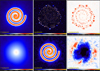 |
Fig. 8. Background derivation (Sect. 3.2) for ℐƛ ≡ 𝒟13″ from Eq. (8). The left panels show the backgrounds ℬƛX and ℬƛY, obtained using the procedure described by Eqs. (20)–(22). The middle panels show the corresponding background-subtracted 𝒮ƛ and ℱƛ from Eq. (23). The right panels show the relative errors of ℬƛX and ℬƛY with respect to the true model backgrounds 𝒟C and 𝒟B (Fig. 2), convolved to the same resolution. The filament is heavily blended with itself in the central area, therefore its background is systematically underestimated there (lower right). Square-root color mapping, except in the right panels, which show linear mapping. |
3.3. Flattening of the structural components
Observations demonstrate that the levels of the large-scale backgrounds and their smaller-scale fluctuations often differ by orders of magnitude in various parts of large images. Although the subtraction of the smooth backgrounds ℬλ{X|Y} greatly simplifies the original images, it does not reduce the strong variations of the smaller-scale fluctuation levels across {𝒮|ℱ}λ. As a consequence, many structures detected with global thresholds in the areas of stronger fluctuations may actually be spurious and unrelated to any real physical objects. On the other hand, faint real structures in the image areas with the lower levels of fluctuations may escape detection because the global threshold value is likely to be overestimated for those areas. To produce complete and reliable extractions using constant thresholds, it is necessary to make small-scale fluctuations uniform over the entire background-subtracted images.
The fluctuation levels are equalized using flattening images 𝒬λ and ℛλ that are derived by getsf from the images 𝒰λ and 𝒱λ of the standard deviations computed in the structural components with a circular sliding window of a radius Oλ,
 (24)
(24)
where 𝒮λR and ℱλR are the regularized images 𝒮λ and ℱλ, obtained using a smoother version of their backgrounds that is median-filtered using a sliding window of a radius 2Oλ and convolved with a Gaussian kernel of a half-maximum size Oλ,
 (25)
(25)
This is done to improve the quality of {𝒰|𝒱}λ for further processing because the structural components from by Eq. (23) are positively defined and have large areas of zero pixels. The regularized components in Eq. (25) acquire small-scale fluctuations resembling the background and noise fluctuations of the original images.
3.3.1. Decomposition of the standard deviations
The advantages of the spatial decomposition (Appendix B) apply also to the standard deviations {𝒰|𝒱}λ. The getsf method produces the single-scales {𝒰|𝒱}λj and employs the same iterative algorithm (Appendix B) to determine the single-scale standard deviation σλj and its total value σλ. This is done using the same procedure as was applied to ℐλ in Sect. 3.2.1.
3.3.2. Removal of the structural features
The {𝒰|𝒱}λ images sample local fluctuations and intensity gradients, revealing all sources and filaments present in ℐλ (Figs. 9 and 10). To produce the corresponding flattening images, it is necessary to remove all such features from {𝒰|𝒱}λ, hence to determine their {X|Y}λ-scale backgrounds. Deriving the latter, getsf creates single-scale slices {𝒰|𝒱}λjl, in a complete analogy with Iλjl in Sect. 3.2.2, and clips from them all source- and filament-like shapes according to their definitions in Eq. (15). The reconstructed backgrounds 𝒬λX and ℛλY are computed using the iterative algorithm described in Sect. 3.2.3, with the largest spatial scale set to 2.5{X|Y}λ.
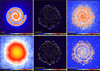 |
Fig. 9. Flattening for the component 𝒮ƛ (Sect. 3.3) for ℐƛ ≡ 𝒟13″ from Eq. (8). The top row shows the original ℐƛ, the background-subtracted 𝒮ƛ from Eq. (23), and the standard deviations 𝒰ƛ from Eq. (24). The bottom row shows the flattening 𝒬ƛ, the flat sources 𝒮ƛD from Eq. (27), and its standard deviations |

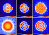 |
Fig. 10. Flattening for the component ℱƛ (Sect. 3.3) for ℐƛ ≡ 𝒟13″ from Eq. (8). The top row shows the original ℐƛ, the background-subtracted ℱƛ from Eq. (23), and the standard deviations 𝒱ƛ from Eq. (24). The bottom row shows the flattening image ℛƛ, the flat filaments ℱƛD from Eq. (27) and its standard deviations |
When the background iterations converge, numerous sharp craters remain in the derived backgrounds {𝒬|ℛ}λ{X|Y} that could create spurious structures if the images were used to flatten the structural components. To avoid this, the final flattening images 𝒬λ and ℛλ (Figs. 9 and 10) are obtained by median filtering the background in circular sliding windows of radii 2Oλ and 5Oλ, respectively,
 (26)
(26)
This important step ensures that flattening would never produce spurious structures in the detection images.
3.3.3. Flattening of the detection images
The detection images of the separated structural components are used to identify peaks of the sources and skeletons of the filaments, respectively (Sect. 3.4). Both source- and filament-detection images are flattened, that is, divided by the flattening images,
 (27)
(27)
The standard deviations  in the regularized flattened components demonstrate that the detection images are remarkably flat outside the structures, as shown in Figs. 9 and 10. This ensures an accurate separation of significant structures from the fainter background and noise fluctuations during the subsequent extraction of sources and filaments.
3.4. Extraction of the structural components
To extract sources and filaments means to detect them and measure their properties. The background subtraction and flattening algorithms presented in Sects. 3.2 and 3.3 radically simplify the originals ℐλ, separating two distinct structural components and creating the independent flat detection images {𝒮|ℱ}λD. In contrast to the originals, the flat images are suitable for the detection techniques that apply a threshold value for the entire image.
3.4.1. Decomposition of the detection images
In order to accurately extract various structures that widely range in brightness and size, it is essential to use the benefits offered by the single-scale spatial decomposition (Appendix B). Following its general approach (Fig. 1, Sects. 3.2.1 and 3.3.1), getsf decomposes the detection images 𝒮λD and ℱλD into single scales {𝒮|ℱ}λDj and estimates the corresponding standard deviations σλSj and σλFj (Appendix B) that are necessary for separating significant structures from all other fluctuations. The decomposed components 𝒮λDj and ℱλDj are shown in Figs. 11 and 12 after they were cleaned and combined over wavebands.
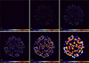 |
Fig. 11. Combination of the detection images 𝒮λDjC (Sect. 3.4.2) for the set of images ℐλ containing all Herschel wavebands and ℐƛ ≡ 𝒟13″ from Eq. (8). The clean 𝒮DjC thresholded above ϖλSj = 5σλSj and combined over all wavebands are shown. Several faint spurious peaks visible on large scales near edges in the bottom row are the background and noise fluctuations that happened to be stronger than the threshold. They may be discarded during the subsequent detection and measurement steps. Logarithmic color mapping. |
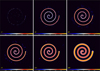 |
Fig. 12. Combination of the detection images ℱƛDjC (Sect. 3.4.2) for the set of images ℐλ containing all Herschel wavebands and ℐƛ ≡ 𝒟13″ from Eq. (8). The clean ℱDjC thresholded above ϖλFj = 2σλFj and combined over five wavebands are shown (excluding the noisier 70 and 100 μm images). The faint ring-like structures that are visible on some scales are the source residuals originating from the derived surface densities that have substantial inaccuracies over the sources (cf. Figs. 5 and 8; Appendix A). Square-root color mapping. |
3.4.2. Cleaning of the single-scale detection images
Cleaning is the removal of insignificant background and noise fluctuations from detection images that needs to be done before combining them over wavebands (Sect. 3.4.3). The clean images of the structures are obtained by preserving only the pixels with values above the cleaning thresholds ϖλ{S|F}j and by setting all fainter pixels to zero,
 (28)
(28)
where ϖλSj = 5σλSj and ϖλFj = 2σλFj. The filament threshold is significantly lower than that for sources because getsf additionally cleans ℱλDjC of the residual source-like clusters of connected pixels according to their definition in Eq. (15).
The resulting clean images {𝒮|ℱ}λDjC (Figs. 11 and 12) are deemed to have signals only from the sources and filaments, respectively. In practice, some of them may have several faint spurious peaks and other structures that are discarded during the subsequent detection and measurement steps.
3.4.3. Combination of the clean single scales over λ
All previous image processing was done independently for each wavelength. It is recommended to always process the input images in parallel, independent getsf runs to reduce the total extraction time approximately by a factor NW, the number of wavelengths. Now, getsf accumulates the clean single-scale images 𝒮λDjC and ℱλDjC over the wavebands in order to use the independent information from all images and enhance the signal of the significant structures. This procedure follows the getold approach (Paper I), with the important improvement that filaments are handled in the same way as sources. When decomposed images on each scale are combined, differences in the angular resolutions between the wavebands are much less important because the single-scale images select and enhance the structures with widths similar to the scale size Sj, not the resolution Oλ.
The clean detection images are normalized before their accumulation over wavelengths to make all cleaning thresholds equal to unity in all bands. The combination process is described by the following expression:
 (29)
(29)
where N{S|F} ≤ NW is the number of the wavebands chosen to be used in the combination, 𝒵λ{S|F}j is the threshold image (equal to ϖλ{S|F}jŌ in all pixels), and fλj is a factor that gradually turns the smallest scales on,
 (30)
(30)
This factor ensures that the small-scale noise or artifacts appearing on top of the resolved structures do not produce spurious detections in the combined images on scales Sj < Oλ. Sufficiently bright unresolved structures still contribute to {𝒮|ℱ}DjC on the smallest scales below Oλ. This super-resolution is useful to detect blended unresolved peaks. Selected combined images of the two structural components are shown in Figs. 11 and 12.
The normalization to a common threshold in Eq. (29) is a natural way of maximizing sensitivity of the combined images. This procedure modifies the original dependence of the source brightness on spatial scales, however, which is analyzed by the detection algorithm (Sect. 3.4.4) to determine the characteristic size for each source. Therefore a second set of combined images is defined for the component of sources, normalized to the smallest scale in each waveband,
 (31)
(31)
where wλ is the weight that enhances the contribution of the images with higher angular resolutions,
 (32)
(32)
where Ō is the average resolution, and the power of 7 ensures complete separation of the contributions of different wavebands in Eq. (31). After the weighting, the summation of 𝒮λDjC preserves the individual dependence of the peak intensity of each source on spatial scales, which provides an initial estimate of its size during detection before the actual measurements.
3.4.4. Detection of sources in the combined images
Sources are detected in 𝒮DjC with almost the same algorithm that was used by getold (Sect. 2.5 of Paper I), which is briefly summarized here for completeness. An inspection of the entire set of single-scale images 𝒮DjC shows that sources appear on relatively small scales become the brightest on scales roughly equal to their size and vanish on significantly larger scales (cf. Fig. B.1). All detectable sources appear isolated on small scales and become blended with other nearby sources on larger scales. The getsf source detection scheme identifies the sources in 𝒮DjC and tracks their evolution from small to large scales, until they disappear or merge with a nearby brighter source.
To detect sources, getsf slices 𝒮DjC by a number NL of intensity levels Ijl, spaced by δlnIj = 0.01, from the image maximum down to the lowest non-zero value. Each slice l cuts through all peaks brighter than Ijl, producing a set of partial images,
 (33)
(33)
The source detection algorithm works on the sequence of partial images, creating and updating source segmentation masks (for each j and l). This is done with the same tintfill algorithm that was applied in Sect. 3.2.2 to remove the source- and filament-like shapes. The resulting single-scale segmentation images of sources set all pixels belonging to a source to its number.
The scale jF on which a source n becomes the brightest is referred to as the footprinting scale. It provides an initial estimate for its half-maximum size Hn = SjF (cf. Appendix B), which defines the initial footprint, that is, the entire area of all pixels making non-negligible contributions to the total flux of the source. From a practical point of view, getsf defines the initial footprint diameter of a circular source as ϕnHn, where the footprint factor ϕn = 3. For the Gaussian sources (e.g., Fig. B.1), these footprints lead to the total fluxes that are underestimated by only 1.6%, well within the usual measurement uncertainties. Having detected the sources, getsf creates their initial footprints with the diameters {A, B}Fn = ϕnHn. The footprints become elliptically shaped in the wavelength-dependent measurements, reflecting the elongation of sources that is obtained from intensity moments. During the measurement iterations (Sect. 3.4.6), getsf changes ϕn to expand or shrink the footprints for those sources that are bright enough and whose intensity distributions indicate that their initial footprints are not optimal.
3.4.5. Detection of filaments in the combined images
Filaments are detected in ℱDjC with a completely new approach. In the getold algorithm (Sect. 2.4.4 of Paper II), intensity profiles at each pixel of the component of filaments are measured in four directions, and the pixel is deemed to belong to the crest (marks a skeleton point) if it has the highest value for each of the profiles. In practice, this simple approach sometimes creates artifacts at the filament end points, where the skeletons sometimes appear forked like a snake tongue. An important limitation of the getold skeletons is that they trace crests of the images of filaments without any dependence on the spatial scales.
The Herschel observations of nearby star-forming molecular clouds demonstrated that filaments are very complex, multiscale structures (e.g., Men’shchikov et al. 2010), unlike the simple case of the relatively round sources, whose intensities rapidly decrease in all directions from their peaks. Resolved sources are produced by the emission of dense, compact objects and may be reasonably well characterized by a single value of their half-maximum size (or spatial scale). In contrast to the sources, detection of filaments is fundamentally a scale-dependent problem, and a single skeleton that may be appropriate for a certain spatial scale cannot fully describe the complexity of the observed multiscale, profoundly substructured filaments. Resolved filaments often appear to be composed of thinner filaments on smaller scales, down to the angular resolution, and their widths, profiles, and crest intensities are quite variable along their skeletons.
The strong dependence of the observed filaments on spatial scales is illustrated in Fig. 13, which shows the surface densities of the filaments in three well-studied star-forming regions: Taurus, Aquila, and IC 5146. The observed images of the regions were downloaded from the Herschel Gould Belt Survey (André et al. 2010) archive4, and the hires surface densities 𝒟13″ of the regions were computed from Eq. (8). Figure 13 shows the images of the spatially decomposed filaments on three selected scales: small, intermediate, and large. The images demonstrate that the observed filaments are highly substructured in the regions, and their shapes as traced by the skeletons are very different on various spatial scales. The skeletons, obtained on the small scales, are completely incompatible with the shapes and crests of the filaments on larger scales. The detected small-scale skeletons are often very curved, meandering back and forth even at the right angles, which implies a high degree of self-blending and leads to significant inaccuracies in the measured profiles and other derived properties of filaments. Therefore it is necessary to detect their skeletons on the scales that correspond to the widths of the structures being studied. Moreover, the small-scale substructures of the larger-scale filaments may even be the key to understanding the filament properties, the physical processes taking place inside them, and the formation of stars.
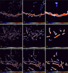 |
Fig. 13. Filaments extracted by getsf on selected spatial scales in three star-forming regions: Taurus (top), Aquila (middle), and IC 5146 (bottom). The flattened components ℱƛD derived from the hires surface densities 𝒟13″ obtained from Eq. (8) using the Herschel 160, 250, 350, and 500 μm images are shown. The minimum scales of 36″ (left column) correspond to 2.8 times the angular resolution, whereas the maximum scales (right column) correspond to 0.3 pc at the adopted distances of the regions (140, 260, and 460 pc, respectively). Intermediate scales between the two extremes are displayed in the middle column. The images were cleaned using the default threshold ϖƛFj = 2σƛFj. Overlaid on the filaments are their skeletons obtained from the images using the Hilditch algorithm (Sect. 3.4.5). The observed filaments are heavily substructured, and their appearance, detected skeletons, and measured properties depend strongly on spatial scales. Logarithmic color mapping. |
Instead of tracing the original image intensity profiles, getsf employs the Hilditch algorithm (Hilditch 1969), which skeletonizes two-dimensional shapes by erasing their outer pixels until the thinnest representation of the shapes is found. The original Hilditch algorithm has a deficiency in that the shapes oriented along the two main diagonals become completely erased during the iterations. To enable its application in getsf, the algorithm has been improved to preserve the diagonal skeletons.
Through the multiscale decomposition, getsf allows finding crests without any explicit analysis of the filament intensities. The single-scale images ℱDjC not only enhance the structures of the widths W ≈ Sj, but also cause these filtered intensity distributions to become well centered on their zero-level footprints. The crests of the isolated decomposed filaments always approximate the medial axes of their footprints (cf. Figs. 12 and 13). If a single-scale filament blends with other filaments (or with itself), there is always a smaller scale on which it is isolated. This allows determining the scale-dependent skeletons as the medial axes of the zero-level filament masks.
The single-scale skeletons 𝒦j are created using the Hilditch algorithm, with a width of three pixels to tolerate one-pixel displacements in the skeleton coordinates between scales. They are further accumulated over a limited range of scales to produce a set of NK skeletons tracing the filamentary structures of various widths,
 (34)
(34)
where J− and J+ are the numbers of the smallest and the largest scales, SJ− = 2−1/2Sk and SJ+ = 2+1/2Sk, in the accumulated skeleton 𝒦k. The scale-dependent skeletons 𝒦k sample the following scales:
 (35)
(35)
where the scale S1 = Ō is defined by Eq. (32) as the average angular resolution over the wavebands combined in ℱDjC (Sect. 3.4.3), and SNK = 4maxλ(Yλ) is the largest spatial scale for the filament detection.
Each pixel of the accumulated skeleton 𝒦k in Eq. (34) contains information on the filament detection significance ξ, defined as the number of scales between J− and J+, on which the single-scale skeleton 𝒦j contributes to 𝒦k in that pixel. Depending on the filament intensity at the skeleton pixel, the significance range is 1 ≤ ξ ≲ ln2 (lnf)−1 (≈14, assuming f ≈ 1.05, Appendix B). The algorithm automatically creates the final one-pixel-wide skeletons by thresholding: 𝒦kξ = max(𝒦k,ξ) with a default ξ = 2, and applying the Hilditch algorithm to the resulting shapes. Segmentation images of the skeletons 𝒦kξ are computed using the tintfill algorithm, which sets all pixels belonging to a filament to its number.
3.4.6. Measurement of the sources
The source-measurement algorithm is an improved version of the one employed by getold (Sect. 2.6 of Paper I). Sources cannot be measured in their component 𝒮λX (Sect. 3.2.3) because the subtracted background ℬλX contains substantial source residuals at low intensity levels (Fig. 8). The background ℬλX is derived specifically for the most complete and reliable source detection, not for accurate measurements. The sources are measured by getsf in the original ℐλ after subtracting their backgrounds and deblending them from overlapping sources, which entails iterations. The background determination and deblending are more accurate for the sources with relatively small footprints. However, in crowded regions with larger areas of overlapping footprints and strongly fluctuating backgrounds, they may become very inaccurate.
The background ℬFλ of each source is determined by a linear interpolation of ℐλ across its footprint. The interpolation along two image axes and two diagonals is based on the adjacent pixels (not belonging to any source) outside the footprint, as was done by getold. To improve the background estimate in the presence of overlapping footprints, getsf evaluates the background only along those of the four directions for which the distances between the outside points being interpolated are within a factor of two of the smallest distance. For each pixel of the source footprint area, the background value is averaged between the directions used in the interpolation. The background ℬFλ is median filtered using a sliding window with a radius Oλ, and the background-subtracted image of a source is then obtained as ℐSλ = ℐλ − ℬFλ.
In the measurements, the source coordinates xn, yn are known from the detection step and are kept unchanged. For the first measurement iteration, it uses the initial characteristic size Hn = SjF, provided by the detection algorithm (Sect. 3.4.4). The corresponding initial footprint {A, B}Fn = ϕnHn is a good approximation for only Gaussian sources, when Hn is close to the actual widths {A, B}λn. However, the initial factor ϕn = 3 may strongly underestimate the footprints of the resolved power-law sources and overestimate those of the resolved flat-topped sources (see below). In the subsequent measurement iterations, the sizes and orientation {A, B, ω}λn from the previous iteration are used.
The size derivation algorithm in getsf has become more accurate, hence it requires some clarifications. The half-maximum sizes were computed by getold using intensity moments (cf. Appendix F in Paper I) that give accurate sizes only for the sources with Gaussian shapes. In real-life observations, however, some sources are markedly non-Gaussian and their intensity moments give either over- or underestimated sizes, corresponding to the levels well below or above the half-maximum intensity.
The inaccuracies of the moment sizes become very large for the resolved sources with power-law intensity distributions. The simulated image of such a source shown in Fig. 14 has a half-maximum size of 10″. However, according to the intensity moments (over the entire image), the model source has a diameter of 76″. It is easy to see that this value corresponds to a level that is lower by an order of magnitude than the half-maximum intensity. The source size depends on the adopted footprint. Within the two footprints shown in the middle and right panels of Fig. 14, the moment sizes are 10.2 and 22.5″. The source flux is also underestimated by correspondingly large factors of 5.2 and 1.8.
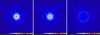 |
Fig. 14. Footprint expansion, illustrated in an image with 3″ resolution of a source with a peak intensity of 100, half-maximum size of 10″, and S/N of 100 (left). The source has an intensity profile defined by Eq. (2) with Θ = 5″ and ζ = 1, transforming into a power law I ∝ θ−2 for θ ≫ Θ and filling up the entire image, its faint outer areas (I ∼ 0.2) are largely lost within the noise. The initial footprint factor ϕn = 3 (Sect. 3.4.4) is too small for these power-law sources, hence background subtraction leaves a relatively bright pedestal containing a large amount of the source emission (middle). The footprint expansion algorithm (Sect. 3.4.6) enlarges ϕn by a factor of 2.2 (right), which lowers the source background by a factor of 5, and as a result, increases the source flux by a factor of 2.7. The improved flux is still below the true value by a factor of 1.9 because the actual footprint is about three times larger. Square-root color mapping. |
Large inaccuracies of the half-maximum sizes also occur for the resolved starless cores that tend to have flat-topped shapes at short wavelengths (λ ≲ 250 μm, cf. Fig. 3), where the emission of their low-temperature interiors fades away. A simulated image of such a source is shown in Fig. 15, with the model half-maximum size of 49″. However, the intensity moments (over the entire image) indicate that its diameter is 31″, which corresponds to a level by a factor of 2 above the half-maximum intensity. In the simple example in Fig. 15, the source size and flux do not depend on the footprint size because the intensity profile in its outer parts is steep and the background is flat (zero).
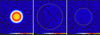 |
Fig. 15. Footprint shrinkage, illustrated in an image with 3″ resolution of a flat-topped source with a peak intensity of 100, half-maximum size of 49″, and S/N of 100 (left), modeled as a 50″ cylinder convolved with a 10″ Gaussian kernel. The initial footprint factor ϕn = 3 (Sect. 3.4.4) is too large for the flat-topped source (middle), whose actual footprint relates to the FWHM value by a factor ϕn = 1.5. The footprint shrinkage algorithm (Sect. 3.4.6) reduces ϕn by a factor of 1.5 (right), which shrinks the footprint and confines it to the pixels belonging to the source alone. This footprint adjustment improves the accuracy of background interpolation and flux measurement on complex backgrounds. Square-root color mapping. |
The above examples demonstrate that the intensity moments do not provide accurate estimates of the half-maximum source sizes in the general case of arbitrary non-Gaussian intensity profiles. Therefore getsf determines accurate half-maximum sizes by the direct Gaussian interpolation of the source intensity distribution at its half-maximum and averaging the resulting distances from the source peak, thereby estimating an average radius hλn. The source elongation EMλn = AMλn/BMλn and position angle ωMλn are computed independently from the intensity moments above the 10% level of the peak, excluding the low-intensity pixels that may be affected by the noise and background fluctuations. The major and minor half-maximum axes of the source are then computed from
 (36)
(36)
where the (empirical) exponential factor converts the average radius hλn into the equivalent-area radius (AλnBλn)1/2 of an ellipse. The FWHM ellipse {A, B, ω}λn from Eq. (36) is guaranteed to correspond to the source half-maximum intensity, in contrast to the ellipse estimated from the intensity moments. The moment sizes {A, B, ω}Mλn are also computed by getsf because they contain independent information that can be useful for the analysis of the extracted sources.
During the measurement iterations (Sect. 2.6 of Paper I), getsf employs a footprint expansion and shrinkage algorithm to correct the footprint areas of those sources that need such adjustments. It is based on a simple observation that when a footprint area is too small, the source background contains a pedestal of the residual intensity distribution of the source (Fig. 14); when the source pedestal does not exist or is negative (Fig. 15), the footprint may be accurate or too large. The analysis is made in the regularized component 𝒮λR from Eq. (25) without contribution from the complex background and filaments.
The presence of the background pedestal is indicated by the positive difference between the background values below the source and those in an external annulus just outside the source,
 (37)
(37)
where BΦλn is the median value within the footprint and BΨλn and DΨλn are the mean and the standard deviation inside the annulus. When the condition of Eq. (37) is fulfilled and the source is not too elongated (Aλn < 1.3Bλn) and bright enough (Ξλn > 50 and Ωλn > 15, see Eq. (41)), getsf increases the factor ϕn by 5% before proceeding to the next measurement iteration. The footprint expansion terminates when the residual background pedestals (Fig. 14) are reduced as much as possible and the condition in Eq. (37) becomes false. As a final adjustment, the footprint is expanded once more by the factor 0.9 + 0.1(ϕn/3) to reduce the residual pedestal.
The footprints of the sources that do not need any expansion are attempted to be reduced in size. It is important to confine the footprints to the most local area occupied by the sources because oversized footprints may strongly decrease the accuracy of background subtraction and flux measurement for sources on complex (filamentary) backgrounds and in crowded areas. The need to shrink a source footprint is indicated by a negative difference between the background values below the source and in an external annulus just outside the source,
 (38)
(38)
where the quantities are the same as in Eq. (37). When the condition of Eq. (38) is fulfilled, getsf decreases the factor ϕn by 2% before proceeding to the subsequent measurement iterations. The footprint shrinkage is completed when the condition in Eq. (38) becomes false, that is, when the reduced footprint causes a small residual background pedestal. In a final adjustment, the footprint is expanded by a factor of 1.1 to eliminate the pedestal created in the process (Fig. 15).
Extensive testing has shown that the simple footprint expansion and shrinkage algorithm performs well for most sources in complicated environments and backgrounds in both benchmarks and real-life observations. Despite the footprint expansion, total fluxes of the power-law sources may still remain underestimated by large factors because the faint outer areas of these sources, with an unknown full extent, vanish into the fluctuating backgrounds and noise.
After computing the background-subtracted images ℐSλ, getsf deblends overlapping sources, calculating the peak intensities FPλn and the total fluxes FTλn for each source n. The iterative deblending algorithm employs the Gaussian shapes Gλn(x, y) defined by the source ellipse {A, B, ω}λn and peak intensity FPλn. The intensity ISλ(x, y) is split between the source n and all overlapping sources n′ according to a fraction of the shape intensities,
 (39)
(39)
where the summation is done over all surrounding sources whose footprints cover the pixel (x, y). The iterative deblending of the peak intensities starts with the original image values ISλ(xn, yn) of each source and proceeds with the splitting of the pixel values until Iλn(xn, yn) converges to the deblended peak intensity FPλn. After obtaining FPλn for all sources, getsf computes the deblended intensities Iλn(x, y) of all pixels within their footprints, estimates the ellipses {A, B, ω}λn and {A, B, ω}Mλn, and integrates the total fluxes FTλn. It also computes an independent flux estimate FGλn by integrating Gλn(x, y), which may only be accurate when a source shape resembles the two-dimensional Gaussian.
Uncertainties of the peak intensities FPλn are estimated by getsf as the standard deviations σPλn, evaluated in the original image ℐλ, in an elliptical annulus around each source n just outside its footprint. In heavily crowded fields, no local source-free annulus can be found near the sources, in which case the uncertainties are estimated from the more distant source-free pixels. The uncertainties σTλn of the total fluxes FTλn are computed with the same assumptions as in getold (Sect. 2.6 of Paper I),
 (40)
(40)
where AFλn and BFλn are the major and minor axes of the source footprints.
It is convenient to define the detection significance Ξλn and the signal-to-noise (S/N) Ωλn and Ψλn, describing the detection and measurement properties of each extracted source,
 (41)
(41)
where jF is the footprinting scale (Sect. 3.4.4) and SλDjFn is the intensity at the source position in 𝒮λDjF (Sect. 3.4.1). The above quantities can be combined together to characterize the overall “goodness” of a source,
 (42)
(42)
normalized such that all acceptable sources in the extraction catalogs have Γλn ≳ 1. The sources with Γλn ≲ 1 may have quite unreliable measurements in waveband λ. The corresponding global quantities Ξn and Γn describe the source detection significance and goodness, respectively, in all wavebands,
 (43)
(43)
The getsf source extraction catalogs contain detailed headers, documenting the extraction parameters and explaining the tabulated quantities. Each data line presents the source number n, coordinates xn, yn (in pixels), world coordinates αn, δn (computed with the xy2sky utility, Mink et al. 2002), global flag fn, significance Ξn, and goodness Γn,
 (44)
(44)
followed (in the same line) by the measured quantities in each of the NW wavebands,
 (45)
(45)
where fλn is a wavelength-dependent flag. In addition to this information, an expanded version of the catalog adds (to the same line) the Gaussian flux FGλn, characteristic size SjF, footprint factor ϕn, and footprint axes AFλn, BFλn. For surface density images, the FGλn column is replaced with source mass Mƛn.
It is necessary to emphasize that sources from extraction catalogs must always be carefully selected (for each waveband separately) to ensure that only sufficiently good and accurately measurable sources are used in further analysis. This is especially important for the multiwavelength extraction catalogs, where sources can be prominent in one waveband and completely undetectable or not measurable in another. The getsf catalogs provide various quantities to enable the evaluation and selection of only acceptable sources and recommended the following selection criteria:
 (46)
(46)
These empirical conditions, based on numerous test results obtained in various benchmarks (Pouteau et al., in prep.; Men’shchikov 2021), and verified in applications to a variety of observed images (e.g., Sect. 4), ensure that the selected subset of sources is reliable (not contaminated by significant numbers of spurious sources) and that selected sources have acceptably accurate measurements.
3.4.7. Measurements of the filaments
Filaments are measured in their background-subtracted ℱλY, derived in Sect. 3.2.3. When the maximum size Yλ of the filaments of interest is estimated sufficiently accurately (Sect. 3.1.3), their background ℬλY does not reveal any filamentary residuals. Nevertheless, the background may well have substantial inaccuracies, especially when the filaments are wide and blended (Fig. 8). Observed filaments are the two-dimensional projections of the complex three-dimensional structures, which are much more difficult to disentangle, deblend, measure, and analyze than sources with their well-defined round shapes and compact footprints.
Sources can be represented by their peak intensity and half-maximum size, but filaments are extremely complicated in their shapes and widths, often interconnected with each other and with various nearby branches, and have variable intensity along their crests. It is quite clear that blending of the structures is a major source of large inaccuracies in the measured quantities of general interest (widths, fluxes, masses, profiles) and in other properties, derived from the measurements.
Another difficulty in understanding filaments (distinct physical structures) is that the filament length cannot be determined objectively. In most cases, it is quite unclear where a physical filament starts, where it ends, and which branches of the three-dimensional filamentary network belong to that filament. Fortunately, the global properties of the entire filaments (even if the latter could be clearly defined) are not as important for studying star formation as the local properties of their relatively short segments that develop appropriate physical conditions for the formation of prestellar cores.
The approach that is adopted in getsf is to simplify the very complex problem by separating all branches of the skeleton network, converting the latter into the simple, non-branching skeletons. The set of non-branching skeletons is derived during the segmentation of the skeletons 𝒦kξ, the last step of the filament detection process (Sect. 3.4.5). The simplified skeletons enable an easy selection and better measurements of only the well-behaving, preferably isolated (not blended), and relatively straight parts of the filaments. No attempt is made by getsf to deblend filaments because a general algorithm for accurately deblending them is not available.
The segmentation image of all skeletons is scanned to trace each skeleton n and find coordinates of all its pixels; to smooth the skeletons, the integer coordinates of their pixels are averaged within a seven-pixel window. The resulting high-resolution coordinates xn(i),yn(i) of each skeleton point i are cataloged, together with the local position angles ϑn(i) of the skeleton direction and αn(i),βn(i) of the left and right normals. A normal is called left (α) or right (β) depending on which side it is located from the first skeleton point to the last. With an adopted distance to the observed region, getsf converts the angular units of the pixels into parsecs and measures each filament as a function of the length l along its skeleton and the distance r along its normals. If the distance is unknown or unspecified, a default distance of 100 pc is used; the measurements can be scaled to another distance after the extraction.
The observed filaments usually meander, hence their skeleton normals diverge from each other on one side and intersect with each other on the other side. In the absence of deblending, more accurate measurements for them are usually obtained from the one-sided quantities that correspond to the side on which the filament is the least affected by blending with itself and with other nearby structures. The filament surface density (or intensity) profiles and their full half-maximum widths are cataloged as the one-sided quantities D{α|β}n(l, r) and W{α|β}n(l) and as the average quantities Dn(l, r) and Wn(l) between the two sides. Also cataloged are the corresponding average profiles D{α|β}n(r) and Dn(r) along the skeleton with their standard deviations ς{α|β}n(r) and ςn(r), as well as the median widths Wn and the slopes γ(r) of the filament profiles.
Although the total length Ln of a skeleton and mass Mn of a filament may not always be objective and physically meaningful quantities (see the discussion above), getsf derives the mass by direct integration of ℱλY within a filament footprint, assuming that the image is obtained from surface densities,
 (47)
(47)
where M{α|β}n are the one-sided mass estimates, from which the average mass Mn between the two sides is obtained. The one-sided footprints Υ{α|β}n used in Eq. (47) are defined as the areas between the skeleton and the maximum extent of the filament on either side. In practice, a filament footprint Υn is the set of all pixels whose shortest distances from the skeleton are smaller than the filament normals.
When the filament mass M{α|β}n and length Ln are known, the one-sided estimates of the average linear density5 of the entire filament are readily obtained,
 (48)
(48)
together with the average linear density  between the two sides. The linear density of filaments is also computed by getsf as a function of the coordinate l along their skeletons,
 (49)
(49)
where the integration limits R{α|β}n(l) along the left and right normals are chosen at zero surface density values or at a radial distance of the profile minimum at which the filament becomes blended with another structure. The median one-sided linear densities Λ{α|β}n for the entire length Ln of the filament and its average linear density Λn are also computed and cataloged. The linear density values from Eqs. (48) and (49) are expected to be similar to each other for the well-behaved filaments.
4. Applications to observed regions
The multiscale, multiwavelength source- and filament-extraction method presented in Sect. 3 was very extensively tested using ∼40 images that were observed with different instruments and both ground-based and orbital telescopes during the past two decades. Multiwaveband observations of star-forming regions obtained in the Herschel Gould Belt Survey (André et al. 2010) and HOBYS (Motte et al. 2010) key projects, as well as the most recent interferometric images observed in the ALMA-IMF program (Motte et al., in prep.), played an important role in validating getsf.
The new extraction method has demonstrated very good results in ALMA benchmarks (Pouteau et al., in prep.) on images, created from a magnetohydrodynamic (MHD) simulation of a star-forming region (Ntormousi & Hennebelle 2019) that was populated with model cores and processed by the casa task simobs (McMullin et al. 2007) to resemble the real ALMA observations (Louvet et al., in prep.). Furthermore, getsf has been applied to source extraction in 15 regions of the ALMA-IMF program and 12 infrared dark clouds of the ASHES survey (Sanhueza et al. 2019; Li et al. 2020). However, the most significant and definitive testing and validation of extraction tools is achieved with simulated benchmarks for which everything is fully known about their components. The second paper (Men’shchikov 2021) presents a quantitative analysis of getsf extractions using several variants of the new benchmark (Sect. 2) and old benchmark (Papers I and III).
Sections 4.1–4.8 illustrate the performance of getsf on nine images obtained with different telescopes: XMM-Newton, the Galaxy Evolution Explorer (GALEX), Hubble, Spitzer, Herschel, the Atacama Pathfinder Experiment (APEX), the James Clerk Maxwell Telescope (JCMT), and ALMA from the X-ray domain to the millimeter wavelengths. These examples are presented to demonstrate that the method is applicable to a wide variety of observed images, visualizing the effects of the separation of structural components and flattening of detection images. Scientific analyses and discussions of these results, as well as their comparisons with previous studies, are beyond the scope of this paper. This can be accomplished using the corresponding extraction catalogs that are available on the getsf website6.
4.1. Supernova remnant RXJ 1713.7−3946
RXJ 1713.7−3946 was observed with XMM-Newton (EPIC camera) in the X-ray waveband (0.6−6 keV) centered at 0.0024 μm. The 0.5° ×0.5° image in Fig. 16 is a mosaic of multiple observations7, first presented in Acero et al. (2017). With an average angular resolution of 7″, it reveals the southeast segment of the supernova remnant shell that may have been created by the explosion of the historical supernova SN 393, whose center of explosion is located beyond the upper right image corner. For this source and filament extraction with getsf, maximum sizes {X|Y}λ = {15, 25}″ were adopted (Sect. 3.1.3).
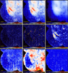 |
Fig. 16. Application of getsf to the XMM-Newtonλ ≈ 0.0024 μm image (7″ resolution) of the supernova remnant RX J1713.7−3946, adopting {X|Y}λ = {15, 25}″. The top row shows the original image ℐλ and the backgrounds ℬλ{X|Y} of sources and filaments. The middle row shows the component 𝒮λ, the footprint ellipses of 41 acceptably good sources on 𝒮λD (red squares mark the spurious peaks), and the component ℱλD with 13 non-branching skeletons 𝒦k2 corresponding to the scales Sk ≈ 40″. The bottom row shows the standard deviations 𝒰λ in the regularized component 𝒮λR, the flattening image 𝒬λ, and the standard deviations in the flattened component |

The observed X-ray image (Fig. 16) has relatively low counts of the detected photons per pixel and high levels of Poisson noise. The image is contaminated by linear artifacts and several spurious single-pixel spikes. The latter may appear in these images when just one or several photons are detected at an edge of the mapped area.
The image features several elongated shock fronts created by the expanding supernova shell, and a number of faint and bright point sources, all of them well isolated. The getsf extraction greatly simplified the image by separating the components of sources 𝒮λ, filaments ℱλ, and their backgrounds ℬλ{X|Y}. The small-scale fluctuation levels across the observed image are only within a factor of two, therefore the improvement caused by the flattening is not clearly discernible in 𝒮λ. However, the images of standard deviations show that the flat source detection image 𝒮λD has uniform fluctuations over the entire image, which is beneficial for source detection.
The extraction catalog contains measurements of 41 sources, all of them selected as acceptably good by Eq. (46). Although the spurious one-pixel spikes were not removed before the extraction, getsf identified them as such (red squares in Fig. 16) and eliminated them from the catalog. Despite the faintness of the observed X-ray image and the Poisson noise, the three prominent shocks of the supernova shell become clearly visible and are extracted in the filament component.
4.2. Star-forming galaxy NGC 6744
NGC 6744 was observed with GALEX in a far-ultraviolet (FUV) waveband (1350−1750 Å) centered at 0.15 μm (Lee et al. 2011). The 0.4° × 0.4° image8 in Fig. 17 with an angular resolution of 4″ shows the spiral galaxy, which is considered to be similar to our own Galaxy. Despite noisiness of the FUV image, it displays the spiral arms with many hundreds of unresolved emission sources. These are the regions of ongoing star formation, heated by the embedded young massive stars. For this source and filament extraction, maximum sizes {X|Y}λ = 20″ were adopted (Sect. 3.1.3).
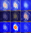 |
Fig. 17. Application of getsf to the GALEX λ = 0.15 μm image (4″ resolution) of the spiral galaxy NGC 6744, adopting {X|Y}λ = 20″. The top row shows the original image ℐλ and the backgrounds ℬλ{X|Y} of sources and filaments. The middle row shows the component 𝒮λ, the footprint ellipses of 1130 acceptably good sources on 𝒮λD, and the component ℱλD with 147 skeletons 𝒦k2 corresponding to the scales Sk ≈ 30″. The bottom row shows the standard deviations 𝒰λ in the regularized component 𝒮λR, the flattening image 𝒬λ, and the standard deviations in the flattened component |

Separation of the structural components by getsf provided independent images of sources 𝒮λ, filaments ℱλ, and their backgrounds ℬλ{X|Y} (Fig. 17). Fluctuation levels in the observed image vary within a factor of two, largely in the central, brighter part of the galaxy. Flattening of the 𝒮λ component effectively equalized the fluctuations across the detection image 𝒮λD, improving the extraction results.
The source catalog contains measurements of 1169 sources, 1130 of which are selected as acceptably good by Eq. (46). Most of the sources likely correspond to the star-forming regions along the galactic spiral arms; many of them overlap with each other, hence they required deblending for accurate measurements of their fluxes. The filaments extracted in the ℱλ component represent the spiral arms and their branches. The 147 skeletons trace the simple, non-branching segments of the filamentary network (Sect. 3.4.5).
4.3. Supernova remnant NGC 6960
NGC 6960 was observed with Hubble in five UVIS wavebands (0.5−0.8 nm) centered at 0.6 μm, within the frame of the Hubble Heritage project (Mack et al. 2015, PI: Z. Levay). The small 73″ × 73″ image9 in Fig. 18 with an angular resolution of 0.2″ represents a small fragment of the Veil Nebula, which is a segment of the Cygnus Loop, the large expanding shell of a supernova remnant (Fesen et al. 2018). For this source and filament extraction with getsf, maximum sizes {X|Y}λ = {0.5, 2}″ were adopted (Sect. 3.1.3).
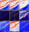 |
Fig. 18. Application of getsf to the Hubbleλ = 0.6 μm image (0.2″ resolution) of the supernova remnant NGC 6960, adopting {X|Y}λ = {0.5, 2}″. The top row shows the original image ℐλ and the backgrounds ℬλ{X|Y} of sources and filaments. The middle row shows the component 𝒮λ, the footprint ellipses of 690 acceptably good sources on 𝒮λD, and the component ℱλD with 100 skeletons 𝒦k2 corresponding to the scales Sk ≈ 1″. The bottom row shows the standard deviations 𝒰λ in the regularized component 𝒮λR, the flattening image 𝒬λ, and the standard deviations in the flattened component |

The observed image (Fig. 18) is dominated by impressive fine filamentary structure of the nebula, seen in emission of a number of atomic lines. Many unresolved intensity peaks of sources are less prominent on this bright backdrop. The structural components were separated by getsf in the independent images of sources 𝒮λ, filaments ℱλ, and backgrounds ℬλ{X|Y}; together with the flattening of detection images, this greatly facilitates their extraction and analysis.
The source catalog contains measurements of 786 sources, 690 of which are selected as acceptably good by Eq. (46). The strings of sources that run up through the middle of the image are the spurious peaks created by the linear artifacts. The spurious spikes were not cut out of the image before this extraction to illustrate that they need to be removed to avoid contamination of the source catalogs. The finely structured filamentary network of the nebula that is extracted by getsf in the ℱλ component comprises 100 skeletons representing its simple, non-branching segments (Sect. 3.4.5).
4.4. Star-forming cloud L 1688
L 1688 was observed with Spitzer in the IRAC 8 μm waveband (Evans et al. 2009). The 1° × 1° image10 in Fig. 19 with an angular resolution of 6″ shows a complex intensity distribution in this well-known star-forming region, with the background varying by almost two orders of magnitude and many sources situated in both faint and bright background areas. For this source and filament extraction with getsf, maximum sizes {X|Y}λ = 30″ were adopted (Sect. 3.1.3).
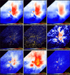 |
Fig. 19. Application of getsf to the Spitzerλ = 8 μm image (6″ resolution) of the L 1688 star-forming cloud, adopting {X|Y}λ = 30″. The top row shows the original image ℐλ and the backgrounds ℬλ{X|Y} of sources and filaments. The middle row shows the component 𝒮λ, the footprint ellipses of 1162 acceptably good sources on 𝒮λD, and the component ℱλD with 286 skeletons 𝒦k2 corresponding to the scales Sk ≈ 30″. The bottom row shows the standard deviations 𝒰λ in the regularized component 𝒮λR, the flattening image 𝒬λ, and the standard deviations in the flattened component |

The clean separation of the components of sources 𝒮λ and filaments ℱλ from their backgrounds ℬλ{X|Y} provided by getsf (Fig. 19) represents an obvious improvement over the results obtained with getimages (Fig. 6 in Paper III). The old method of background derivation was indiscriminate with respect to the shapes of the components, hence the background-subtracted image also contained some filamentary structures on small scales. In contrast to getimages, which produced a single background, getsf derived and subtracted individual backgrounds for 𝒮λ and ℱλ. The component 𝒮λ of sources (Fig. 19) is completely free of the elongated structures. The standard deviations 𝒰λ reveal that the small-scale background fluctuation levels vary by roughly three orders of magnitude across the image. If not equalized, the fluctuations would be extracted as numerous spurious sources and contaminate the source catalog. The very effective flattening of the detection image 𝒮λD leads to a much more reliable extraction.
Several bright unresolved sources in the lower part of the observed image have very wide power-law wings and cross-like artifacts that are induced by the complex PSF of the Spitzer IRAC camera at 8 μm. Their intensity profiles are markedly non-Gaussian, and for a proper measurement of their integrated fluxes, getsf expanded their footprints by factors ∼4–15 using the footprint expansion algorithm (Fig. 14). The cross-like artifacts from the PSF were interpreted by getsf as filaments and were moved to the filament component, thereby improving 𝒮λD for source detection. In addition to the cross shape, the complex PSF has ∼20 faint peaks that surround the main beam. They were extracted as several spurious sources, surrounding the brightest peaks; they must be eliminated in a post-extraction analysis.
The source catalog gives measurements of 1474 sources, 1162 of which are selected as acceptably good using Eq. (46). The filament component produced by getimages (Fig. 7 in Paper III) contains only the brightest parts of the filaments, their fainter intensities are missing. In contrast, getsf determines the intensity distributions down to very low intensity levels, with 286 skeletons tracing the simple, non-branching segments of the filaments (Sect. 3.4.5).
4.5. Embedded starless core L 1689B
L 1689B, one of the nearest well-resolved starless cores (a distance of 140 pc) embedded in a resolved filament, was observed with Herschel in five PACS and SPIRE wavebands (Ladjelate et al. 2020). The 160−500 μm images11 and Eq. (8) were used to compute a 1.1° × 1.1° surface density image 𝒟13″ in Fig. 20 with a resolution of 13.5″ to illustrate the new extraction method on a single image. In addition to the reduction of the number of images, the use of surface densities allows getsf to catalog physical parameters of the core and filament. For this extraction, maximum sizes {X|Y}ƛ = {90,180}″ were adopted (Sect. 3.1.3).
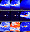 |
Fig. 20. Application of getsf to the Herschel surface density (13.5″ resolution) of the starless core L 1689B, embedded in a filament, adopting {X|Y}λ = {90, 180}″. The top row shows the original hires image 𝒟13″ obtained from Eq. (8) and the backgrounds ℬλ{X|Y} of sources and filaments. The middle row shows the component 𝒮λ, the footprint ellipses of 12 acceptably good sources on 𝒮λD, and the component ℱλD with one skeleton 𝒦k2 corresponding to the scales Sk ≈ 200″. The bottom row shows the standard deviations 𝒰λ in the regularized component 𝒮λR, the flattening image 𝒬λ, and the standard deviations in the flattened component |

The 𝒟13″ image in Fig. 20 presents L 1689B in the wide filamentary structure near the edge of a diffuse cloud, all components are blended. The filament surface density is a factor of ∼5 below the peak surface density NH2 = 3.7 × 1022 cm−2, whereas at the values, lower by just a factor of 2, a round shape of the source becomes distorted by its complex environment. Separation of the components by getsf greatly simplifies the image, isolating the structures in their individual images 𝒮ƛ, ℱƛ, and ℬƛ{X|Y} (Fig. 20). Subsequent flattening of the small-scale fluctuation levels allowed a reliable identification of the filament and sources in both low- and high-background areas of the observed image. The extraction catalog contains measurements of 20 sources, 12 of which are selected as acceptably good by Eq. (46). The single skeleton was obtained on spatial scales of ∼200″, corresponding to the maximum width Yƛ.
The main physical parameters of the starless core L 1689B, M = 0.6 M⊙ and NH2 = 1022 cm−2, are underestimated because of the inaccuracies (Appendix A) of the standard surface density derivation approach (Sect. 3.1.2). The errors and correction factors can be found using the benchmark models from Sect. 2.2. A model of the critical Bonnor–Ebert sphere with TBE = 14 K, M = 1 M⊙, and NH2 = 2.5 × 1022 cm−2 has an FWHM size of 57″, almost the same as the size A = 58″ of L 1689B, measured by getsf. However, in the derived 𝒟13″ image, the same model has M = 0.66 M⊙ and NH2 = 1022 cm−2, implying correction factors of 1.5 and 2.5 for the mass and peak surface density, correspondingly. After correction, the measured mass of L 1689B becomes M ≈ 0.9 M⊙; masses of the other sources in the image are lower by (at least) a factor of ∼10 . The filament measurements (Sect. 3.4.7) give its median value N0 = 3.8 × 1021 cm−2, length L = 0.8 pc, half-maximum width W = 0.14 pc (205″), mass M = 15 M⊙, and linear density Λ = 14 M⊙ pc−1; the values are little affected by the fitting inaccuracies.
4.6. Star-forming cloud NGC 6334
NGC 6334 was observed with APEX at 350 μm, equipped with the ArTéMiS camera (André et al. 2016). The 0.5° ×0.5° image12 in Fig. 21 with an angular resolution of 8″ represents an improvement by a factor of 3 with respect to the Herschel images at 350 μm. Subtraction of the correlated sky noise resulted in an image without signals on spatial scales above 120″ (André et al. 2016). Therefore the large-scale background and the zero level of the image are not known, and the structures in the image are smaller than the largest scale. Fortunately, these observational problems are entirely unimportant for getsf. For this source and filament extraction, maximum sizes {X|Y}λ = 30″ were adopted (Sect. 3.1.3).
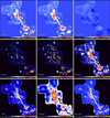 |
Fig. 21. Application of getsf to the APEX λ = 350 μm image (8″ resolution) of the NGC 6334 star-forming cloud, adopting {X|Y}λ = 30″. The top row shows the original image ℐλ and the backgrounds ℬλ{X|Y} of sources and filaments. The middle row shows the component 𝒮λ, the footprint ellipses of 91 acceptably good sources on 𝒮λD, and the component ℱλD with 26 skeletons 𝒦k2 corresponding to the scales Sk ≈ 30″. The bottom row shows the standard deviations 𝒰λ in the regularized component 𝒮λR, the flattening image 𝒬λ, and the standard deviations in the flattened component |

The observed image of NGC 6334 displays complex blended structures of various shapes and intensities (Fig. 21), including substantial numbers of negative areas and artifacts from the data reduction and map-making algorithms. The separated 𝒮λ component shows all source-like peaks very clearly, even those that are hardly visible in the original image, because getsf is able to distinguish sources from the elongated filamentary shapes. Many of the sources overlap each other, therefore they require deblending for accurate measurements. The background ℬλY of filaments is fairly low, hence its subtraction enhanced the visibility of filaments in ℱλ only little. Nonuniform small-scale fluctuations in 𝒮λ were effectively equalized in the detection image 𝒮λD by the flattening algorithm.
The source catalog contains measurements of 124 sources, 91 of which are selected as acceptably good by Eq. (46). In the component of filaments, getsf identified 26 skeletons, tracing the simple, non-branching segments of the filaments (Sect. 3.4.5) on spatial scales of ∼30″, corresponding to the maximum width Yλ.
4.7. Star-forming cloud Orion A
Orion A was observed with JCMT at 450 and 850 μm with the SCUBA-2 camera (Lane et al. 2016) with angular resolutions of 9.8 and 14.6″, respectively. The 0.86° ×0.86° image13 at 850 μm in Fig. 22 displays the northern part of the integral-shaped filament (ISF). Like with other ground-based submillimeter observations that must subtract sky background, large-scale emission in the images has been filtered out (Kirk et al. 2018). A visual estimate suggests that the image contains substantial signal on spatial scales of up to ∼100″. For the two-wavelength getsf extraction, employing both 450 and 850 μm images, maximum sizes {X|Y}{450|850} = {20, 30, 30, 45}″ were adopted (Sect. 3.1.3).
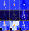 |
Fig. 22. Application of getsf to the JCMT λ = 850 μm image (14.6″ resolution) of the Orion A star-forming cloud, adopting {X|Y}λ = 30″. The top row shows the original image ℐλ and the backgrounds ℬλ{X|Y} of sources and filaments. The middle row shows the component 𝒮λ, the footprint ellipses of 212 acceptably good sources on 𝒮λD, and the component ℱλD with 199 skeletons 𝒦k2 corresponding to the scales Sk ≈ 39″. The bottom row shows the standard deviations 𝒰λ in the regularized component 𝒮λR, the flattening image 𝒬λ, and the standard deviations in the flattened component |

The 850 μm image of the ISF in Fig. 22 reveals the small-scale structures of the area most clearly because of the spatial filtering effect of the observational technique. However, the central bright part of the ISF remains blended, and the spatial decomposition by getsf helps isolate the sources 𝒮λ in that area from the filaments ℱλ and their backgrounds ℬλ{X|Y}. The background of filaments is found to be slightly negative, except in its central bright round area. In comparison with an average value of small-scale fluctuations in 𝒮λ, they are larger by a factor of 2.7 in the central zone and lower by a factor of 1.7 in the lower right corner. The standard deviations 𝒰λ reveal imprints of the five overlapping scans from the observations. The flattening algorithm of getsf effectively equalizes them and creates the flat detection images {𝒮|ℱ}λD of sources and filaments, improving their detection reliability.
The two-band source extraction in ISF with getsf cataloged 344 sources, detected and measured in both wavebands simultaneously. Only 257 and 212 sources at 450 and 850 μm, respectively, are selected as acceptably good by Eq. (46); the S/N for the remaining detections is too low or they have other defects that are identified by the measurements. Two additional getsf extractions, done on each image independently, resulted in catalogs with 319 and 283 sources at 450 and 850 μm, respectively. Independent extractions ignore the valuable information from the other image, hence there are higher chances of spurious sources. With the additional condition that cataloged sources must be detected in both images, the combined extraction catalog contains 223 sources; 196 and 183 of these sources at 450 and 850 μm, respectively, are acceptably good. They represent the most reliable sources in the images, hence it is highly unlikely that there are spurious sources among them.
The missing large-scale emission of the SCUBA-2 image helped getsf expose the many relatively faint, narrow filaments within the wide, massive ISF. In the ℱλ component, getsf identified 267 and 199 simple, non-branching segments of the filaments (Sect. 3.4.5) at 450 and 850 μm, respectively, on transverse scales of 28 and 39″. This is similar to the existence of narrow sub-filaments on small scales within the resolved Taurus, Aquila, and IC 5146 filaments (Fig. 13) and consistent with the recent ALMA observations of ISF (Hacar et al. 2018).
4.8. Star-forming cloud W 43-MM1
W 43-MM1 was observed with the 12 m array of the ALMA interferometer (baselines 13−1045 m) in the 233 GHz band centered at 1300 μm (Motte et al. 2018; Nony et al. 2020). The small 68″ × 68″ image in Fig. 23 with an angular resolution of 0.44″ contains spatial scales of up to 12″, beyond which the interferometer was insensitive to the emission. For this source and filament extraction with getsf, the maximum size {X|Y}λ = {0.8, 1.3}″ was adopted (Sect. 3.1.3).
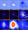 |
Fig. 23. Application of getsf to the ALMA λ =1300 μm image (0.44″ resolution) of the W43-MM1 star-forming cloud, adopting {X|Y}λ = {0.8, 1.3}″. The top row shows the original image ℐλ and the backgrounds ℬλ{X|Y} of sources and filaments. The middle row shows the component 𝒮λ, the footprint ellipses of 44 acceptably good sources on 𝒮λD, and the component ℱλD with 15 skeletons 𝒦k2 corresponding to the scales Sk ≈ 2″. The bottom row shows the standard deviations 𝒰λ in the regularized component 𝒮λR, the flattening image 𝒬λ, and the standard deviations in the flattened component |

The interferometric image of W 43-MM1 (Fig. 23) shows a cluster of relatively bright sources, some of them blended, and three faint filamentary structures that appear to connect them. Separation of the components of sources 𝒮λ and filaments ℱλ confirms that most sources are concentrated on (or near) the faint continuous filaments. Almost the entire background ℬλY of the filamentary structures is negative, which is caused by the missing large scales in the observed images.
The small-scale fluctuation levels steeply increase toward the image center by more than an order of magnitude (Fig. 23), as evidenced by the standard deviations 𝒰λ. The small-scale structured noise from the interferometric observations have both round or irregular, elongated shapes. Consequently, the separation of structural components by getsf leads to many faint peaks in 𝒮λ and ℱλ. The flattening algorithm equalizes the fluctuation levels very effectively, providing reliable detection of sources in the flat {𝒮|ℱ}λD. If not suppressed, such highly variable structured noise would produce many spurious sources and filaments in the central area of the image.
This ALMA image of W43-MM1 contains only moderate numbers of sources and filaments. The extraction catalog contains measurements of 44 sources, and all of them are selected as acceptably good by Eq. (46). This simple field allows a visual verification that they all are the true sources and are not contaminated by the noise fluctuations. In the filament component, getsf identified 15 skeletons, tracing the simple, non-branching segments of the filaments (Sect. 3.4.5) on spatial scales of ∼2″, similar to the maximum width Yλ adopted for the extraction.
5. Strengths and limitations
5.1. Strengths
In contrast to the other methods, getsf extracts sources and filaments simultaneously by combining available information from all wavebands. Its flexible multiwavelength design enables handling of up to 99 images, not necessarily all of them observed in different wavebands. The maximum number of images is arbitrary, representing the largest two-digit integer number used in the output file names; the code can be updated to use a higher value if required for some applications. Any subset of the input images that is deemed beneficial for the detection purposes can be used to detect the sources and filaments, whereas measurements of the identified structures are provided for all input images. In a nonstandard application, the method can also be employed with the position-velocity cubes if they are split into separate images along the velocity axis (getold was used in this way by Shimajiri et al. 2019).
The images that are selected for detection are spatially decomposed to isolate the contributions of similar scales (Appendix B) and are then combined in a wavelength-independent set of single-scale detection images (Sect. 3.4.3). This eliminates the necessity of associating independent detections across wavelengths in images with greatly different angular resolutions and improves the detection and measurement accuracy. For example, positional association of nearby sources detected at 160 μm and completely blended into a single clump at 500 μm does not make sense.
Separation of structural components in the images of highly structured observed regions in space provides independent images of sources, filaments, and their backgrounds (Sect. 3.2), which is highly beneficial for the analysis and interpretation of observations. Flattening of detection images equalizes the (nonuniform) small-scale background and noise fluctuations (Sect. 3.3). This greatly simplifies the images and allows reliable detection of sources and filaments in decomposed single-scale images using a constant threshold, with a very low rate of spurious sources.
Sources and filaments of any size and width can be extracted by getsf provided that they are significantly smaller than the image. Only the maximum size of the structures of interest must be specified for each image in order to limit the range of spatial scales considered and the size of the structures to be measured and cataloged. The single parameter of the observed images that getsf needs to know is the maximum size, which is determined from the images by users (Sect. 3.1.3) on the basis of their research interests. This single constrained parameter reduces the dependence of the extraction results on the human factor to a minimum and makes their analysis and derived conclusions as objective as possible.
The numerical code is designed to be user-friendly and easy to run, providing diagnostics to help users avoid common problems. It verifies the getsf configuration, input images, and masks for consistency, and it suggests solutions in various circumstances during extractions. The software includes 21 utilities and scripts (Appendix C), providing all kinds of image processing necessary for getsf to run and more. They include the fitfluxes utility for spectral energy distribution fitting of source fluxes or image pixels (and mass derivation) and the hires script that computes the high-resolution surface density images (Sect. 3.1.2). Most of the utilities are very useful for command-line image manipulations, even without source and filament extractions.
5.2. Limitations
The method is designed and expected to work for the images that are not very sparse: most pixels must contain detectable signals (measurable data). Examples of the images for which getsf might not produce reliable results are some extremely faint X-ray or UV low-count images with isolated spiking pixels that are surrounded by large areas of pixels that were not assigned any detectable signal. For such nonstandard images, getsf would still work and complete extractions, but its results might not be reliable because the method relies on the standard deviations of the background or noise fluctuations outside structures, whose values may not correctly represent the statistics of the observed data in these images. On the other hand, the images for getsf extractions must not be extremely smooth: they must have some variations on scales of about the angular resolution. However, such smooth images can easily be made perfectly suitable for getsf just by adding Gaussian noise at some faint level that does not alter the structures of interest.
Separation of sources from filaments is not (and cannot be) perfect. It leaves very faint residuals of sources that end up in the filament component. In practice, this is not important because most of the residuals are too faint (Fig. 12) to affect the filament properties. The background of very wide and/or overlapping filaments is likely to be derived less accurately than that of the narrower and/or isolated filaments because the filaments are separated from the wider background areas. Filaments that are separated from wider background peaks of comparable widths are likely to receive some contribution from the background (Fig. 8). In very rare cases, the footprint of a bright power-law peak might not be sufficiently expanded, which leads to an underestimated flux.
The method takes quite considerable time to complete extractions, although getsf was optimized to run as fast as possible. The aim of its design was to produce extraction results that are as reliable as possible because completeness and accuracy, not speed, are of prime importance in astrophysical research. The runtime for the getsf applications presented in Sect. 4 is in the range of three hours to a week (the images with 4302 to 20002 pixels and file sizes of 800 KB to 16 MB). The two-wavelength extraction of sources and filaments for the subfield of Orion A described in Sect. 4.7 took 43 h and required ∼10 GB of disk space. The total processing time with getsf depends on the numbers of pixels, wavelengths, iterations, detected sources and filaments, and on the processor and file system speed and load. A source extraction run on eight large images, each with 48002 pixels (92 MB file size), that detects and measures ∼3000 sources, may need about three weeks and ∼200 GB of disk space. Most of the time getsf spends in the iterative separation of structural components: the actual extraction of sources and filaments takes less than 10% of the runtime. For the source extraction alone, the execution time is halved. In a properly planned research, the processing time is almost never a limiting factor: much more time is usually spent on the analysis and interpretation of the information delivered by the extraction and on describing the findings in a paper.
Many intermediate images are produced in the getsf extractions at each wavelength (for spatial decomposition, iterations, etc.), hence they require large storage space. Between hundreds of MB and GB may be necessary for an extraction, depending on the image size and the numbers of wavebands and iterations. It is necessary to keep many images until the end of the extraction process; however, most of them may be deleted by getsf after the extraction has finished. The extraction results themselves represent only ∼20% of the total size of the extraction directory. Computers with sufficiently large random access memory are required to run getsf extractions on very large images. For the above range of image sizes, between 8 and 64 GB may be necessary (the more memory, the better). The actual memory usage strongly depends on the number of sources being detected and measured. Numbers of sources up to ∼15 000 do not pose any problems to getsf, but substantially larger numbers of detected sources require very large memory and long execution time.
6. Conclusions
This paper presented getsf, the new multiscale method for extracting both sources and filaments in astronomical images using separation of their structural components. It is specifically designed to handle multiwavelength sets of images and extremely complex filamentary backgrounds, but it is perfectly applicable to a single image or very simple backgrounds. The new code is freely downloadable from its website14, from the Astrophysics Source Code Library15, and also available from the author.
The main processing steps of getsf include (1) preparation of a complete set of images and derivation of high-resolution surface densities, (2) spatial decomposition of the original images and separation of the structural components of sources and filaments from each other and from their backgrounds, (3) flattening of the residual noise and background fluctuations in the separate images of sources and filaments, (4) spatial decomposition of the flattened components of sources and filaments and their combination of the over wavelengths, (5) detection of sources (positions) and filaments (skeletons) in the combined images of the components, and (6) measurements of the properties of the detected sources and filaments and creation of the output catalogs and images. Like its predecessor (getold, Papers I–III), getsf has a single user-definable parameter (per wavelength), the maximum size of the structures of interest to extract. All internal parameters of getsf have been calibrated and verified in numerous tests using various images from simulations and observations to ensure that the method works well in all cases.
This paper formulated hires, the algorithm for the derivation of high-resolution surface densities and temperatures from the diffraction-limited multiwavelength far-infrared and submillimeter continuum observations, such as those obtained with Herschel. A substantial improvement over the original algorithm (Palmeirim et al. 2013) is the angular resolution of the derived surface densities that may become as high as that of the shortest-wavelength image of a sufficient quality. In the case of the Herschel observations, the resolution may be as high as 5.6″ for the slow scanning speed (20″ s−1) or 8.4″ for the fast parallel mode (60″ s−1). If the 70 μm image appears too noisy, excessively contaminated by the emission of polycyclic aromatic hydrocarbons or transiently heated very small dust grains, or if it cannot be used for other reasons, then the highest resolution of surface densities is limited to that of the 100 or 160 μm images, that is, to 6.8−11.3″ or 8.4−13.5″, for the slow- or fast-scanning modes, respectively. These high-resolution surface density images are especially useful for the detailed studies of the highly complex structural diversity in the observed images and for deeper understanding of the physical processes within the heavily substructured filaments and their relation to the formation of stars.
This paper described the set of simulated multiwavelength benchmark images for testing and comparing the source and filament extraction methods to allow the researchers who need to perform such extractions to choose the most accurate algorithm for their projects. Although the benchmark was designed to resemble the Herschel observations of star-forming regions, the images are suitable for testing and evaluating extraction methods for any astronomical projects and applications. It consists of the complex fluctuating background cloud, the long dense filament, and many starless and protostellar cores with wide ranges of sizes, masses, and intensity profiles, computed with a radiative transfer code. A separate paper (Men’shchikov 2021) presents a series of the multiwavelength source extractions with getsf using three variants of the new benchmark with increasing complexity levels and compares their results with those produced by getold. All benchmark images, the truth catalogs containing the model parameters, and the reference extraction catalogs obtained by the author with getsf are available on its website.
The new extraction method can be used to conduct consistent and comparable studies of sources and filaments in various projects: getsf is designed to work for all images with nonzero background or noise fluctuations, where most pixels carry nonzero measured signal. The method is not limited to any particular area of astronomical research nor to the type of the telescopes or instruments used, as demonstrated by its applications to the images obtained with XMM-Newton, GALEX, Hubble, Spitzer, Herschel, APEX, and ALMA. Although no finite numbers of specific examples can prove that getsf is universally applicable, they confirm a remarkably wide applicability of the method.
In some publications, the filament linear density is also referred to as the mass per unit length.
Acknowledgments
This study used the cfitsio library (Pence 1999), developed at HEASARC NASA (USA), saoimage ds9 (Joye & Mandel 2003) and wcstools (Mink et al. 2002), developed at the Smithsonian Astrophysical Observatory (USA), and the stilts library (by Mark Taylor), developed at Bristol University (UK). The plot utility and ps12d library, used in this work to draw figures directly in the PostScript language, were written by the author using the psplot library (by Kevin E. Kohler), developed at Nova Southeastern University Oceanographic Center (USA), and the plotting subroutines from the MHD code azeus (Ramsey et al. 2012), developed by David Clarke and the author at Saint Mary’s University (Canada). This work used observations obtained with XMM-Newton, an ESA science mission with instruments and contributions directly funded by ESA Member States and NASA. This work used observations made with the Spitzer Space Telescope, which is operated by the Jet Propulsion Laboratory, California Institute of Technology, under a contract with NASA. This work used observations made with the NASA/ESA Hubble Space Telescope, and obtained from the Hubble Legacy Archive, which is a collaboration between the Space Telescope Science Institute (STScI/NASA), the Space Telescope European Coordinating Facility (ST-ECF/ESA) and the Canadian Astronomy Data Centre (CADC/NRC/CSA). This paper used the SCUBA-2 data obtained at JCMT under program MJLSG31. The James Clerk Maxwell Telescope is operated by the East Asian Observatory on behalf of The National Astronomical Observatory of Japan; Academia Sinica Institute of Astronomy and Astrophysics; the Korea Astronomy and Space Science Institute; Center for Astronomical Mega-Science (as well as the National Key R&D Program of China with No. 2017YFA0402700). Additional funding support is provided by the Science and Technology Facilities Council of the United Kingdom and participating universities and organizations in the United Kingdom and Canada. Additional funds for the construction of SCUBA-2 were provided by the Canada Foundation for Innovation. This paper used the following ALMA data: ADS/JAO.ALMA#2013.1.01365.S. ALMA is a partnership of ESO (representing its member states), NSF (USA) and NINS (Japan), together with NRC (Canada), NSC and ASIAA (Taiwan), and KASI (Republic of Korea), in cooperation with the Republic of Chile. The Joint ALMA Observatory is operated by ESO, AUI/NRAO and NAOJ. The simulated surface density background ℬ was derived from a synthetic scale-free background image created by Ph. André. A large set of images, used for testing and validation of getsf, includes those obtained in the Herschel Gould Belt Survey (http://gouldbelt-herschel.cea.fr) (HGBS, PI Ph. André), HOBYS (http://hobys-herschel.cea.fr) (PIs F. Motte, A. Zavagno, S. Bontemps), and ALMA-IMF (PIs F. Motte, A. Ginsburg, F. Louvet, P. Sanhoueza). HGBS and HOBYS are the Herschel Key Projects jointly carried out by SPIRE Specialist Astronomy Group 3 (SAG3), scientists of several institutes in the PACS Consortium (e.g., CEA Saclay, INAF-IAPS Rome, LAM/OAMP Marseille), and scientists of the Herschel Science Center (HSC). The author appreciates the valuable feedback, received from G. Zhang, F. Louvet, and N. Kumar, on the getsf extractions in the X-shaped nebula, MHD simulations, and Mon R2, respectively. The author is grateful to A. Zavagno, T. Nony, Y. Shimajiri, Ph. André, D. Arzoumanian, and P. Palmeirim for their comments on the manuscript.
References
- Abràmoff, M. D., Magalhães, P. J., & Ram, S. J. 2004, Biophoton. Internatl., 11, 36 [Google Scholar]
- Acero, F., Katsuda, S., Ballet, J., & Petre, R. 2017, A&A, 597, A106 [NASA ADS] [CrossRef] [EDP Sciences] [Google Scholar]
- André, P., Men’shchikov, A., Bontemps, S., et al. 2010, A&A, 518, L102 [NASA ADS] [CrossRef] [EDP Sciences] [Google Scholar]
- André, P., Revéret, V., Könyves, V., et al. 2016, A&A, 592, A54 [NASA ADS] [CrossRef] [EDP Sciences] [Google Scholar]
- Aniano, G., Draine, B. T., Gordon, K. D., & Sandstrom, K. 2011, PASP, 123, 1218 [NASA ADS] [CrossRef] [Google Scholar]
- Arzoumanian, D., André, P., Didelon, P., et al. 2011, A&A, 529, L6 [CrossRef] [EDP Sciences] [Google Scholar]
- Arzoumanian, D., André, P., Könyves, V., et al. 2019, A&A, 621, A42 [NASA ADS] [CrossRef] [EDP Sciences] [Google Scholar]
- Berry, D. S. 2015, Astron. Comput., 10, 22 [NASA ADS] [CrossRef] [Google Scholar]
- Bertin, E., Mellier, Y., Radovich, M., et al. 2002, in Astronomical Data Analysis Software and Systems XI, eds. D. A. Bohlender, D. Durand,&T. H. Handley, ASP Conf. Ser., 281, 228 [Google Scholar]
- Black, J. H. 1994, in The First Symposium on the Infrared Cirrus and Diffuse Interstellar Clouds, eds. R. M. Cutri, & W. B. Latter, ASP Conf. Ser., 58, 355 [Google Scholar]
- Bouwman, J. 2001, PhD thesis, University of Amsterdam, The Netherlands [Google Scholar]
- Clark, S. E., Peek, J. E. G., & Putman, M. E. 2014, ApJ, 789, 82 [Google Scholar]
- Evans, N. I., Jr, Dunham, M. M., Jørgensen, J. K., et al. 2009, ApJS, 181, 321 [NASA ADS] [CrossRef] [Google Scholar]
- Fesen, R. A., Weil, K. E., Cisneros, I. A., Blair, W. P., & Raymond, J. C. 2018, MNRAS, 481, 1786 [Google Scholar]
- Hacar, A., Tafalla, M., Forbrich, J., et al. 2018, A&A, 610, A77 [NASA ADS] [CrossRef] [EDP Sciences] [Google Scholar]
- Hennemann, M., Motte, F., Schneider, N., et al. 2012, A&A, 543, L3 [NASA ADS] [CrossRef] [EDP Sciences] [Google Scholar]
- Hilditch, C. J. 1969, in Machine Intelligence, eds. B. Meltzer, & D. Michie, 4, 403 [Google Scholar]
- Joye, W. A., & Mandel, E. 2003, in Astronomical Data Analysis Software and Systems XII, eds. H. E. Payne, R. I. Jedrzejewski, & R. N. Hook, ASP Conf. Ser., 295, 489 [NASA ADS] [Google Scholar]
- Juvela, M. 2016, A&A, 593, A58 [NASA ADS] [CrossRef] [EDP Sciences] [Google Scholar]
- Kirk, J. M., Ward-Thompson, D., Palmeirim, P., et al. 2013, MNRAS, 432, 1424 [NASA ADS] [CrossRef] [Google Scholar]
- Kirk, H., Hatchell, J., Johnstone, D., et al. 2018, ApJS, 238, 8 [CrossRef] [Google Scholar]
- Koch, E. W., & Rosolowsky, E. W. 2015, MNRAS, 452, 3435 [NASA ADS] [CrossRef] [Google Scholar]
- Könyves, V., André, P., Men’shchikov, A., et al. 2015, A&A, 584, A91 [NASA ADS] [CrossRef] [EDP Sciences] [Google Scholar]
- Ladjelate, B., André, P., Könyves, V., et al. 2020, A&A, 638, A74 [CrossRef] [EDP Sciences] [Google Scholar]
- Lane, J., Kirk, H., Johnstone, D., et al. 2016, ApJ, 833, 44 [NASA ADS] [CrossRef] [Google Scholar]
- Lee, J. C., de Gil Paz, A., Kennicutt, R. C., Jr., et al. 2011, ApJS, 192, 6 [NASA ADS] [CrossRef] [Google Scholar]
- Li, S., Sanhueza, P., Zhang, Q., et al. 2020, ApJ, 903, 119 [Google Scholar]
- Mack, J., Levay, Z. G., Christian, C. A., et al. 2015, Hubble Heritage Project [Google Scholar]
- McMullin, J. P., Waters, B., Schiebel, D., Young, W., & Golap, K. 2007, in Astronomical Data Analysis Software and Systems XVI, eds. R. A. Shaw, F. Hill, & D. J. Bell, ASP Conf. Ser., 376, 127 [Google Scholar]
- Men’shchikov, A. 2013, A&A, 560, A63 [NASA ADS] [CrossRef] [EDP Sciences] [Google Scholar]
- Men’shchikov, A. 2016, A&A, 593, A71 [NASA ADS] [CrossRef] [EDP Sciences] [Google Scholar]
- Men’shchikov, A. 2017, A&A, 607, A64 [NASA ADS] [CrossRef] [EDP Sciences] [Google Scholar]
- Men’shchikov, A. 2021, A&A, submitted [Google Scholar]
- Men’shchikov, A., André, P., Didelon, P., et al. 2010, A&A, 518, L103 [NASA ADS] [CrossRef] [EDP Sciences] [Google Scholar]
- Men’shchikov, A., André, P., Didelon, P., et al. 2012, A&A, 542, A81 [NASA ADS] [CrossRef] [EDP Sciences] [Google Scholar]
- Mink, D. J. 2002, in Astronomical Data Analysis Software and Systems XI, eds. D. A. Bohlender, D. Durand, & T. H. Handley, ASP Conf. Ser., 281, 169 [Google Scholar]
- Molinari, S., Schisano, E., Faustini, F., et al. 2011, A&A, 530, A133 [NASA ADS] [CrossRef] [EDP Sciences] [Google Scholar]
- Motte, F., André, P., & Neri, R. 1998, A&A, 336, 150 [Google Scholar]
- Motte, F., André, P., Ward-Thompson, D., & Bontemps, S. 2001, A&A, 372, L41 [NASA ADS] [CrossRef] [EDP Sciences] [Google Scholar]
- Motte, F., Zavagno, A., Bontemps, S., et al. 2010, A&A, 518, L77 [NASA ADS] [CrossRef] [EDP Sciences] [Google Scholar]
- Motte, F., Nony, T., Louvet, F., et al. 2018, Nat. Astron., 2, 478 [NASA ADS] [CrossRef] [Google Scholar]
- Nony, T., Motte, F., Louvet, F., et al. 2020, A&A, 636, A38 [CrossRef] [EDP Sciences] [Google Scholar]
- Ntormousi, E., & Hennebelle, P. 2019, A&A, 625, A82 [EDP Sciences] [Google Scholar]
- Ossenkopf, V., & Henning, T. 1994, A&A, 291, 943 [NASA ADS] [Google Scholar]
- Palmeirim, P., André, P., Kirk, J., et al. 2013, A&A, 550, A38 [NASA ADS] [CrossRef] [EDP Sciences] [Google Scholar]
- Parravano, A., Hollenbach, D. J., & McKee, C. F. 2003, ApJ, 584, 797 [NASA ADS] [CrossRef] [Google Scholar]
- Pence, W. 1999, in Astronomical Data Analysis Software and Systems VIII, eds. D. M. Mehringer, R. L. Plante, & D. A. Roberts, ASP Conf. Ser., 172, 487 [Google Scholar]
- Press, W. H., Teukolsky, S. A., Vetterling, W. T., & Flannery, B. P. 1992, Numerical recipes in FORTRAN. The art of scientific computing, 2nd edn. (Cambridge: Cambridge University Press) [Google Scholar]
- Ramsey, J. P., Clarke, D. A., & Men’shchikov, A. B. 2012, ApJS, 199, 13 [NASA ADS] [CrossRef] [Google Scholar]
- Rosolowsky, E. W., Pineda, J. E., Kauffmann, J., & Goodman, A. A. 2008, ApJ, 679, 1338 [NASA ADS] [CrossRef] [Google Scholar]
- Sanhueza, P., Contreras, Y., Wu, B., et al. 2019, ApJ, 886, 102 [NASA ADS] [CrossRef] [Google Scholar]
- Schisano, E., Rygl, K. L. J., Molinari, S., et al. 2014, ApJ, 791, 27 [NASA ADS] [CrossRef] [Google Scholar]
- Shimajiri, Y., André, P., Ntormousi, E., et al. 2019, A&A, 632, A83 [NASA ADS] [CrossRef] [EDP Sciences] [Google Scholar]
- Smith, A. R. 1979, SIGGRAPH’79: Proc. of the 6th Annual Conference on Computer Graphics and Interactive Techniques (New York: ACM), 276 [Google Scholar]
- Sousbie, T. 2011, MNRAS, 414, 350 [NASA ADS] [CrossRef] [Google Scholar]
Appendix A: Inaccuracies of the derived surface densities and temperatures
The algorithms described in Sect. 3.1.2 imply that the 160, 250, 350, and 500 μm images have an accurate (consistent) intensity calibration. When we assume that the calibration inaccuracies can be described by constant wavelength-dependent offsets, simple consistency checks and corrections can be made. Three independent estimates of low-resolution temperatures (𝒯L1, 𝒯L2, 𝒯L3) are readily available from fitting the images in three pairs of wavebands (160−250, 250−350, and 350−500 μm) with a low resolution of O500. If the median values of the three temperature maps differ by more than several percent, it would be necessary to adjust some of the offsets and estimate 𝒯L{1|2|3} again. This iterative process is stopped when the three temperatures become consistent.
The higher-resolution images are obtained at the cost of significantly stronger noise and greater chances of distortions and spurious peaks. The quality of the resulting {𝒟|𝒯}P from Eq. (5) strongly depends on the quality of the original short-wavelength images. Higher levels of noise or map-making artifacts in the 250 and 160 μm images would be amplified in the resulting maps in the process of fitting the spectral shapes Πλ of pixels, which is likely to create significant small-scale distortions, predominantly in the pixels with strong line-of-sight temperature gradients that are usually located over the dense sources or filaments. The differential terms δ{𝒟|𝒯}{3|2} that contain the higher-resolution information are increasingly less accurate because they are obtained from fitting of only three and two (noisier) images. It is very important to carefully inspect {𝒟|𝒯}P to ensure that they are free of spurious small-scale structures before using them in any extraction. The hires images {𝒟|𝒯}OH from Eqs. (8) and (11) are much less affected by the problems because they use the contributions δ{𝒟|𝒯}{4|3|2} from all three variants of the fitted temperatures for each of the six resolutions of the original images.
The essential idea of the differential algorithm for improving the angular resolution of surface density was validated using the benchmark images (Sect. 2). The complete surface density 𝒟C + 𝒟S was first convolved to the resolutions of all Herschel wavebands (Sect. 2.3). The algorithm of Eq. (5), generalized to all six wavebands, was then applied to improve the lowest-resolution surface density using the unsharp masking of Eq. (6) and to successively recover each of the higher-resolution surface densities, all the way up to the highest adopted resolution O70 = 8.4″, with a resulting maximum error below 0.5%. Although this is an excellent accuracy of the scheme, real-life applications of the method involve fitting of the spectral pixel shapes Πλ, hence they inevitably suffer from larger inaccuracies (Fig. A.1).
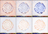 |
Fig. A.1. Relative accuracies ϵ of the hires surface densities and temperatures derived from Eq. (8) (Sect. 3.1.2) with respect to the true model images convolved to the same resolutions. The top row shows the errors in 𝒟8″ (σ = 0.15), 𝒟18″ (σ = 0.06), and 𝒟36″ (σ = 0.05) and the bottom row shows the errors in 𝒯8″ (σ = 0.06), 𝒯18″ (σ = 0.05), and 𝒯36″ (σ = 0.05). At the highest resolution of 8″, the derived images are the most accurate, with the exception of the unresolved protostellar peak surface densities (Fig. 3), which become strongly overestimated (up to a factor of ∼10) because the temperatures 𝒯{2|3|4} along the lines of sight with large temperature gradients are underestimated. The range of displayed values is reduced for better visibility. Linear color mapping. |
The derived surface densities 𝒟P and 𝒟OH (Sect. 3.1.2) are not suitable for measuring dense structures, especially those with a central source of heating, because their inaccuracies in the pixels with strong line-of-sight temperature gradients are too large (e.g., Men’shchikov 2016). Comparisons with the true surface densities in Fig. A.1 show that the vast majority of the pixels outside bright sources are quite accurate, to better than 0.5%. However, the inaccuracies become much larger in the places that are occupied by the sources with steep gradients of the line-of-sight temperature. The starless cores and protostellar envelopes have markedly different radial temperature profiles, therefore the errors that are induced in the derived surface densities are also very dissimilar in both their sign and magnitude.
Appendix B: Single-scale spatial decomposition and standard deviations
Following the getold general approach, getsf employs successive unsharp masking to decompose the prepared original images ℐλ (Sect. 3.1.1) into NS single scales,
 (B.1)
(B.1)
where 𝒢j are the circular Gaussian convolution kernels (𝒢0 is to be regarded as the delta function) with progressively increasing half-maximum sizes,
 (B.2)
(B.2)
where f > 1 is the discretization factor (typically f ≈ 1.05) and the limiting scales of the decomposition range are
 (B.3)
(B.3)
where Δ is the pixel size. The first image ℐλ1 contains the contribution from all scales below Smin, whereas the last image ℐλNS does not contain the signals from the scales above Smax, they are outside the range of scales being analyzed. The convolution is done with rescaling to conserve the total flux, hence the originals ℐλ can be recovered by summation of the NS scales and all remaining largest spatial scales,
 (B.4)
(B.4)
The spatial decomposition is illustrated in Fig. B.1 using an example of a simple two-dimensional Gaussian shape 𝒫. As demonstrated in Papers I and II, the spatial decomposition has many useful properties. The filtered single-scale images contain signals from a relatively narrow range of spatial scales, and their properties resemble the Gaussian statistics much better than those of the originals, which are blends of all spatial scales. On the scales much smaller than the image size, the decomposed images are well described by the global value of the standard deviation σλj. Significant departures from the Gaussian distribution in single scales above a certain threshold (e.g., Iλj ≳ 5σλj) indicate the presence of the real structures. The decomposition highlights the structures of a specific width in the decomposed images on a matching scale. For example, a resolved isolated circular source with a half-maximum size Hλ has its maximum brightness in ℐλj on the scale Sj ≈ Hλ and a completely unresolved source produces the brightest signal on the smallest spatial scales Sj ≲ Oλ.
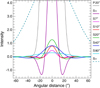 |
Fig. B.1. Single-scale spatial decomposition for an unresolved source 𝒫 with a peak value of 100 and resolution Oλ = 20″ into 99 scales between Smin = 7″ and Smax = 80″, with the scale factor f = 1.026. The profiles of the original Gaussian are shown for the six selected single scales (from S < Smin to Smax), and of the largest scales (𝒢99 * 𝒫), outside the decomposition range (S > Smax). |
Following the getold approach (Papers I and II), getsf employs an iterative algorithm to determine the single-scale σλj over the entire usable area ℐλjℳλ of the image to separate the real structures from other insignificant background or noise fluctuations. Before the iterations, the global σλj0 and the threshold ϖλj0 = 3σλj0 are computed over all pixels. At the first and all subsequent iterations (i = 1, 2, …, NI), significant peaks and hollows with |Iλj|≥ϖλji − 1 are masked. The absolute value is taken, because structures have both positive and negative counterparts in the decomposed images. Then getsf calculates a new (lower) σλji value outside the masked areas and all structures with |Iλj|≥ϖλji are masked again. The iterations continue until the threshold converges to a stable value of ϖλji, with corrections δϖλji < 1%. The final single-scale standard deviation is obtained as σλj = ϖλj/3 and its total value as  . The constant 3, chosen empirically, provides both suitable values of the resulting σλj values and good convergence of the iterations.
A notable difference with getold is that getsf does not need to correct the iterated thresholds using the higher-order statistical moments (skewness and kurtosis) because significant structures are detected in accurately flattened detection images (Sect. 3.4), which ensures that the majority of pixels resemble a normal distribution. Furthermore, precise σλj values are of relatively minor importance for the separation of structural components because the separation is done in iterations and is based on the shapes that are removed from the single-scale slices (Sect. 3.2.2), not on the σλj value itself.
Appendix C: Software suite
The method has been developed as a bash script getsf that executes a number of FORTRAN utilities, doing all numerical computations. Linux or macOS systems with the ifort or gfortran compilers can be used to install the code. For reading and writing images, getsf uses the cfitsio library (Pence 1999); for resampling and reprojecting images, it calls swarp (Bertin et al. 2002); for convolving images, it uses the fast Fourier transform routine rlft3 (Press et al. 1992); for determining the source coordinates α and δ, it applies xy2sky from wcstools (Mink et al. 2002); and for a colored screen output, it uses the highlight utility (by André Simon)16, if the latter is installed.
The following list of the getsf utilities and scripts explains their purpose and functions. They are quite useful for command-line image manipulations, even if there is no need in a source or filament extraction. Their usage information is displayed when a utility is run without any parameter. The utilities are sorted in the decreasing sequence of their general usability outside getsf.
| modfits | modify an image or its header in various ways: math transformations; profiling an image along a line; image segmentation; filament skeletonization; removal of connected clusters of pixels; addition or removal of border areas; correction of saturated or bad pixel areas; conversion of intensity units; changes of the header keywords; etc. |
| operate | operate on two input images: addition, subtraction, multiplication, division; relative differencing; minimization or maximization; extension or expansion of masks; copying of an image header; computation of surface densities, temperatures, or intensities; etc. |
| imgstat | display and/or save image statistical quantities; produce mode-, mean-, or median-filtered images; compute images of standard deviations, skewness, kurtosis; etc. |
| fftconv | fast Fourier transform or convolve image with few predefined kernels or an external kernel image |
| fitfluxes | fit spectral shapes of source fluxes or image pixel intensities to derive masses or surface densities |
| convolve | convolve an image to a desired lower resolution |
| resample | resample and reproject an image with rotation |
| hires | high-resolution surface densities and temperatures |
| prepobs | convert observed images into the same pixel grid |
| installg | install getsf on a computer (macOS, Linux) |
| iospeed | test I/O speed of a hard drive for a specific image |
| readhead | display an image header or save selected keywords |
| cleanbg | interpolate background below source footprints |
| ellipses | overlay an image with ellipses of extracted sources |
| sfinder | detect sources in combined single-scale images |
| smeasure | measure and catalog properties of detected sources |
| fmeasure | measure and catalog properties of detected filaments |
| finalcat | produce the final catalogs of detected sources |
| expanda | expand masked areas of an image to its edges |
| extractx | extract all image extensions in separate images |
| splitcube | split a data cube into separate images |
The code is automated, flexible, and user-friendly; it can be downloaded from the website17, the Astrophysics Source Code Library18, and it is also available from the author upon request. The website also contains a detailed User’s Guide and a complete validation extraction of sources and filaments in a small image for those who would like to verify that their installed getsf produces correct results.
All Figures
|
Fig. 1. Flowchart of the image processing steps in getsf. The colored blocks represent preparation (purple), background subtraction (blue), image flattening (green), and extraction of sources and filaments (red). |
| In the text | |
|
Fig. 2. Background surface densities (𝒟B, 𝒟C) and average line-of-sight dust temperatures (𝒯C) used to compute the simulated Herschel images 𝒞λ of the filamentary cloud from Eq. (4). Square-root color mapping. |
| In the text | |
|
Fig. 3. Component of sources 𝒮λ that is composed of the images of radiative transfer models of 828 starless and 91 protostellar cores and convolved to the Herschel resolutions Oλ (cf. Sect. 1), shown at three selected wavelengths. Only the bright unresolved emission peaks of the protostellar cores, clearly visible at 100 μm, appear in the 70 μm image (not shown). Square-root color mapping. |
| In the text | |
|
Fig. 4. Images ℋλ of the simulated star-forming region, defined by Eq. (1)), shown at three selected wavelengths. The benchmark images are a superposition of four structural components: the background ℬλ, the filament ℱλ, the sources 𝒮λ, and the noise 𝒩λ. Two simpler variants of this benchmark are also available: without the filament and without the background. Square-root color mapping. |
| In the text | |
|
Fig. 5. Derived surface densities and temperatures (Sect. 3.1.2). The true model image 𝒟C + 𝒟S and the hires surface density 𝒟13″ and temperature 𝒯13″ derived from Eq. (8) with λH = 160 μm (OH = 13.5″) are shown. Many of the sources, clearly visible in the true image (left), are not discernible in the derived surface density (middle) because of the inaccuracies in the temperatures from fitting spectral shapes Πλ. Square-root color mapping, except the right panel with linear mapping. |
| In the text | |
|
Fig. 6. High-resolution surface densities obtained for the Herschel images of Cygnus X (HOBYS project, Motte et al. 2010; Hennemann et al. 2012; Bontemps et al., in prep.). The top row shows the hires surface densities 𝒟OH from Eq. (8) with OH = 18.2″ and 5.9″ resolutions, and the high-contrast |
| In the text | |
|
Fig. 7. Spatial decomposition (Sect. 3.2.1, Appendix B) for ℐƛ ≡ 𝒟13″ from Eq. (8) in single scales between 4 and 1400″. The original hires surface density (top left) and decomposed ℐƛj on selected scales Sj that differ by a factor of 4 are plotted. The remaining largest scales 𝒢NS∗ℐƛ (bottom right) are outside the decomposition range. Linear color mapping. |
| In the text | |
|
Fig. 8. Background derivation (Sect. 3.2) for ℐƛ ≡ 𝒟13″ from Eq. (8). The left panels show the backgrounds ℬƛX and ℬƛY, obtained using the procedure described by Eqs. (20)–(22). The middle panels show the corresponding background-subtracted 𝒮ƛ and ℱƛ from Eq. (23). The right panels show the relative errors of ℬƛX and ℬƛY with respect to the true model backgrounds 𝒟C and 𝒟B (Fig. 2), convolved to the same resolution. The filament is heavily blended with itself in the central area, therefore its background is systematically underestimated there (lower right). Square-root color mapping, except in the right panels, which show linear mapping. |
| In the text | |
|
Fig. 9. Flattening for the component 𝒮ƛ (Sect. 3.3) for ℐƛ ≡ 𝒟13″ from Eq. (8). The top row shows the original ℐƛ, the background-subtracted 𝒮ƛ from Eq. (23), and the standard deviations 𝒰ƛ from Eq. (24). The bottom row shows the flattening 𝒬ƛ, the flat sources 𝒮ƛD from Eq. (27), and its standard deviations |
| In the text | |
|
Fig. 10. Flattening for the component ℱƛ (Sect. 3.3) for ℐƛ ≡ 𝒟13″ from Eq. (8). The top row shows the original ℐƛ, the background-subtracted ℱƛ from Eq. (23), and the standard deviations 𝒱ƛ from Eq. (24). The bottom row shows the flattening image ℛƛ, the flat filaments ℱƛD from Eq. (27) and its standard deviations |
| In the text | |
|
Fig. 11. Combination of the detection images 𝒮λDjC (Sect. 3.4.2) for the set of images ℐλ containing all Herschel wavebands and ℐƛ ≡ 𝒟13″ from Eq. (8). The clean 𝒮DjC thresholded above ϖλSj = 5σλSj and combined over all wavebands are shown. Several faint spurious peaks visible on large scales near edges in the bottom row are the background and noise fluctuations that happened to be stronger than the threshold. They may be discarded during the subsequent detection and measurement steps. Logarithmic color mapping. |
| In the text | |
|
Fig. 12. Combination of the detection images ℱƛDjC (Sect. 3.4.2) for the set of images ℐλ containing all Herschel wavebands and ℐƛ ≡ 𝒟13″ from Eq. (8). The clean ℱDjC thresholded above ϖλFj = 2σλFj and combined over five wavebands are shown (excluding the noisier 70 and 100 μm images). The faint ring-like structures that are visible on some scales are the source residuals originating from the derived surface densities that have substantial inaccuracies over the sources (cf. Figs. 5 and 8; Appendix A). Square-root color mapping. |
| In the text | |
|
Fig. 13. Filaments extracted by getsf on selected spatial scales in three star-forming regions: Taurus (top), Aquila (middle), and IC 5146 (bottom). The flattened components ℱƛD derived from the hires surface densities 𝒟13″ obtained from Eq. (8) using the Herschel 160, 250, 350, and 500 μm images are shown. The minimum scales of 36″ (left column) correspond to 2.8 times the angular resolution, whereas the maximum scales (right column) correspond to 0.3 pc at the adopted distances of the regions (140, 260, and 460 pc, respectively). Intermediate scales between the two extremes are displayed in the middle column. The images were cleaned using the default threshold ϖƛFj = 2σƛFj. Overlaid on the filaments are their skeletons obtained from the images using the Hilditch algorithm (Sect. 3.4.5). The observed filaments are heavily substructured, and their appearance, detected skeletons, and measured properties depend strongly on spatial scales. Logarithmic color mapping. |
| In the text | |
|
Fig. 14. Footprint expansion, illustrated in an image with 3″ resolution of a source with a peak intensity of 100, half-maximum size of 10″, and S/N of 100 (left). The source has an intensity profile defined by Eq. (2) with Θ = 5″ and ζ = 1, transforming into a power law I ∝ θ−2 for θ ≫ Θ and filling up the entire image, its faint outer areas (I ∼ 0.2) are largely lost within the noise. The initial footprint factor ϕn = 3 (Sect. 3.4.4) is too small for these power-law sources, hence background subtraction leaves a relatively bright pedestal containing a large amount of the source emission (middle). The footprint expansion algorithm (Sect. 3.4.6) enlarges ϕn by a factor of 2.2 (right), which lowers the source background by a factor of 5, and as a result, increases the source flux by a factor of 2.7. The improved flux is still below the true value by a factor of 1.9 because the actual footprint is about three times larger. Square-root color mapping. |
| In the text | |
|
Fig. 15. Footprint shrinkage, illustrated in an image with 3″ resolution of a flat-topped source with a peak intensity of 100, half-maximum size of 49″, and S/N of 100 (left), modeled as a 50″ cylinder convolved with a 10″ Gaussian kernel. The initial footprint factor ϕn = 3 (Sect. 3.4.4) is too large for the flat-topped source (middle), whose actual footprint relates to the FWHM value by a factor ϕn = 1.5. The footprint shrinkage algorithm (Sect. 3.4.6) reduces ϕn by a factor of 1.5 (right), which shrinks the footprint and confines it to the pixels belonging to the source alone. This footprint adjustment improves the accuracy of background interpolation and flux measurement on complex backgrounds. Square-root color mapping. |
| In the text | |
|
Fig. 16. Application of getsf to the XMM-Newtonλ ≈ 0.0024 μm image (7″ resolution) of the supernova remnant RX J1713.7−3946, adopting {X|Y}λ = {15, 25}″. The top row shows the original image ℐλ and the backgrounds ℬλ{X|Y} of sources and filaments. The middle row shows the component 𝒮λ, the footprint ellipses of 41 acceptably good sources on 𝒮λD (red squares mark the spurious peaks), and the component ℱλD with 13 non-branching skeletons 𝒦k2 corresponding to the scales Sk ≈ 40″. The bottom row shows the standard deviations 𝒰λ in the regularized component 𝒮λR, the flattening image 𝒬λ, and the standard deviations in the flattened component |
| In the text | |
|
Fig. 17. Application of getsf to the GALEX λ = 0.15 μm image (4″ resolution) of the spiral galaxy NGC 6744, adopting {X|Y}λ = 20″. The top row shows the original image ℐλ and the backgrounds ℬλ{X|Y} of sources and filaments. The middle row shows the component 𝒮λ, the footprint ellipses of 1130 acceptably good sources on 𝒮λD, and the component ℱλD with 147 skeletons 𝒦k2 corresponding to the scales Sk ≈ 30″. The bottom row shows the standard deviations 𝒰λ in the regularized component 𝒮λR, the flattening image 𝒬λ, and the standard deviations in the flattened component |
| In the text | |
|
Fig. 18. Application of getsf to the Hubbleλ = 0.6 μm image (0.2″ resolution) of the supernova remnant NGC 6960, adopting {X|Y}λ = {0.5, 2}″. The top row shows the original image ℐλ and the backgrounds ℬλ{X|Y} of sources and filaments. The middle row shows the component 𝒮λ, the footprint ellipses of 690 acceptably good sources on 𝒮λD, and the component ℱλD with 100 skeletons 𝒦k2 corresponding to the scales Sk ≈ 1″. The bottom row shows the standard deviations 𝒰λ in the regularized component 𝒮λR, the flattening image 𝒬λ, and the standard deviations in the flattened component |
| In the text | |
|
Fig. 19. Application of getsf to the Spitzerλ = 8 μm image (6″ resolution) of the L 1688 star-forming cloud, adopting {X|Y}λ = 30″. The top row shows the original image ℐλ and the backgrounds ℬλ{X|Y} of sources and filaments. The middle row shows the component 𝒮λ, the footprint ellipses of 1162 acceptably good sources on 𝒮λD, and the component ℱλD with 286 skeletons 𝒦k2 corresponding to the scales Sk ≈ 30″. The bottom row shows the standard deviations 𝒰λ in the regularized component 𝒮λR, the flattening image 𝒬λ, and the standard deviations in the flattened component |
| In the text | |
|
Fig. 20. Application of getsf to the Herschel surface density (13.5″ resolution) of the starless core L 1689B, embedded in a filament, adopting {X|Y}λ = {90, 180}″. The top row shows the original hires image 𝒟13″ obtained from Eq. (8) and the backgrounds ℬλ{X|Y} of sources and filaments. The middle row shows the component 𝒮λ, the footprint ellipses of 12 acceptably good sources on 𝒮λD, and the component ℱλD with one skeleton 𝒦k2 corresponding to the scales Sk ≈ 200″. The bottom row shows the standard deviations 𝒰λ in the regularized component 𝒮λR, the flattening image 𝒬λ, and the standard deviations in the flattened component |
| In the text | |
|
Fig. 21. Application of getsf to the APEX λ = 350 μm image (8″ resolution) of the NGC 6334 star-forming cloud, adopting {X|Y}λ = 30″. The top row shows the original image ℐλ and the backgrounds ℬλ{X|Y} of sources and filaments. The middle row shows the component 𝒮λ, the footprint ellipses of 91 acceptably good sources on 𝒮λD, and the component ℱλD with 26 skeletons 𝒦k2 corresponding to the scales Sk ≈ 30″. The bottom row shows the standard deviations 𝒰λ in the regularized component 𝒮λR, the flattening image 𝒬λ, and the standard deviations in the flattened component |
| In the text | |
|
Fig. 22. Application of getsf to the JCMT λ = 850 μm image (14.6″ resolution) of the Orion A star-forming cloud, adopting {X|Y}λ = 30″. The top row shows the original image ℐλ and the backgrounds ℬλ{X|Y} of sources and filaments. The middle row shows the component 𝒮λ, the footprint ellipses of 212 acceptably good sources on 𝒮λD, and the component ℱλD with 199 skeletons 𝒦k2 corresponding to the scales Sk ≈ 39″. The bottom row shows the standard deviations 𝒰λ in the regularized component 𝒮λR, the flattening image 𝒬λ, and the standard deviations in the flattened component |
| In the text | |
|
Fig. 23. Application of getsf to the ALMA λ =1300 μm image (0.44″ resolution) of the W43-MM1 star-forming cloud, adopting {X|Y}λ = {0.8, 1.3}″. The top row shows the original image ℐλ and the backgrounds ℬλ{X|Y} of sources and filaments. The middle row shows the component 𝒮λ, the footprint ellipses of 44 acceptably good sources on 𝒮λD, and the component ℱλD with 15 skeletons 𝒦k2 corresponding to the scales Sk ≈ 2″. The bottom row shows the standard deviations 𝒰λ in the regularized component 𝒮λR, the flattening image 𝒬λ, and the standard deviations in the flattened component |
| In the text | |
|
Fig. A.1. Relative accuracies ϵ of the hires surface densities and temperatures derived from Eq. (8) (Sect. 3.1.2) with respect to the true model images convolved to the same resolutions. The top row shows the errors in 𝒟8″ (σ = 0.15), 𝒟18″ (σ = 0.06), and 𝒟36″ (σ = 0.05) and the bottom row shows the errors in 𝒯8″ (σ = 0.06), 𝒯18″ (σ = 0.05), and 𝒯36″ (σ = 0.05). At the highest resolution of 8″, the derived images are the most accurate, with the exception of the unresolved protostellar peak surface densities (Fig. 3), which become strongly overestimated (up to a factor of ∼10) because the temperatures 𝒯{2|3|4} along the lines of sight with large temperature gradients are underestimated. The range of displayed values is reduced for better visibility. Linear color mapping. |
| In the text | |
|
Fig. B.1. Single-scale spatial decomposition for an unresolved source 𝒫 with a peak value of 100 and resolution Oλ = 20″ into 99 scales between Smin = 7″ and Smax = 80″, with the scale factor f = 1.026. The profiles of the original Gaussian are shown for the six selected single scales (from S < Smin to Smax), and of the largest scales (𝒢99 * 𝒫), outside the decomposition range (S > Smax). |
| In the text | |
Current usage metrics show cumulative count of Article Views (full-text article views including HTML views, PDF and ePub downloads, according to the available data) and Abstracts Views on Vision4Press platform.
Data correspond to usage on the plateform after 2015. The current usage metrics is available 48-96 hours after online publication and is updated daily on week days.
Initial download of the metrics may take a while.