© The Authors 2023

1 Introduction

Astronomical imaging with modern telescopes and interferometers provide ever increasing angular resolutions and sensitivities. Observed images contain distinct structural components, such as interstellar clouds, filaments, and sources. All of those structures are the integral parts of the dynamically interacting interstellar matter, controlled by the gravity and other physical processes, which play important roles in the formation of stars. Observationally, the filaments are significantly elongated structures and the sources are relatively round peaks in the images, which stand out of (and blend with) the complex fluctuations of the clouds and small-scale instrumental noise. The observed sources and filaments are produced by various physical objects in the interstellar clouds. Because of their integral nature, separation of the sources from the filaments and from the background clouds is a nontrivial problem. In the regions that are not too distant from the Galactic plane, the backgrounds are quite bright, have complex structures, and strongly fluctuate on all spatial scales, as demonstrated in the recent decades by the well-known sensitive, high-resolution images obtained with Hubble, Spitzer, and Herschel.

The currently available resolutions are rarely sufficient to fully resolve the imaged sources and filaments in distant regions – relatively large point-spread functions (PSFs) of the telescopes blur the physical objects, artificially widening their true angular sizes. Although the higher sensitivities (lower noise levels) of newer instruments enable detection of fainter structures, they also reveal more complex fluctuating backgrounds that complicate the extraction and accurate measurements of the structures of interest. In general, an extracted source or filament does not contain emission of just a single physical object, but very often it is a blend of background fluctuations and other nearby objects. Assessing their physical properties requires accurate methods of background subtraction, deblending, and deconvolution of the observed structures. Such reliable methods are presently unavailable, as manifested by the major problems with the physical properties derived for the unresolved sources in both observations and numerical simulations, reported by Louvet et al. (2021). They showed that the numbers, sizes, and masses of the sources extracted at different angular resolutions linearly depend on the resolution and, as a result, the peak of the source mass function shifts to lower masses. The effects were attributed to the heavy blending of the sources with filaments and a background cloud as well as to an inaccurate background determination at lower angular resolutions.

A simple approach to deconvolving the half maximum size s of a structure from its measured half maximum size w in an image convolved with a kernel of a half maximum size k relies on the basic mathematical property of convolution (w² = s² + k²), which is valid only for the Gaussian shapes of both the kernel and the object. Because of its simplicity, the method is widely used to deconvolve the sizes of both sources (e.g., Motte et al. 2003; Bontemps et al. 2010; Nguyen Luong et al. 2011; Könyves et al. 2015; Ladjelate et al. 2020; Pouteau et al. 2022) and filaments (e.g., Arzoumanian et al. 2011, 2019; Palmeirim et al. 2013; André et al. 2016; Cox et al. 2016). In the astronomical studies, this simple Gaussian size deconvolution method implies strictly Gaussian shapes of the telescope PSFs, the extracted (background-subtracted) structures, and the corresponding physical objects, constituting a strong set of conditions.

In reality, the PSFs of orbital telescopes are flatter and more complex than a Gaussian shape, affected by the diffraction rings and spikes, at angular distances from their centers larger than roughly their half maximum widths. Even if the beams were Gaussian, most astrophysical objects would have non-Gaussian (often power-law) shapes beyond their peaks, at least the objects of common interest in star-forming molecular clouds, such as the dense filaments and prestellar or protostellar cores. Even if both the beams and the objects had Gaussian shapes, just a slightly inaccurate subtraction of the fluctuating backgrounds of the structures would make them have non-Gaussian profiles.

Backgrounds of observed sources and filaments are blends of the interstellar clouds and instrumental noise that display complex fluctuations on the spatial scales of and above the observational beam. To make the problem tractable, it makes sense to somewhat simplify the complexity of background shapes and assume that, in general, the structures have chances to be situated on the flat, convex (hill-like), or concave (bowl-like) background fluctuations. An unknown background of a specific source or filament must be subtracted, which has the potential to strongly affect the measured sizes, peak intensities, and integrated fluxes of the objects, and hence their derived masses. Benchmark extractions indicate that errors in the integrated fluxes of faint sources within a factor of ~2 are fairly common, reaching even factors of up to an order of magnitude in some cases (cf. Figs. 6–10 and A.1 in Men’shchikov 2021a).

From a physical point of view, the embedded dense cores and elongated structures, forming inside a molecular cloud, are expected to spatially coincide with significant volume density enhancements because the objects are created by their self-gravity (along with other processes). This implies higher chances for such sources and filaments of being observed on the local volume density peaks, although the latter would not necessarily appear as the surface density peaks (e.g., Padoan et al. 2023). Depending on the angular resolution and projected volume density variations along the lines of sight, backgrounds of the observed structures may have approximately convex or concave shapes and, in the simplest cases, the backgrounds might also be flat.

The structures with shallower power-law profiles, occupying wider image areas, have higher chances of blending with the nonuniform backgrounds of complex shapes. It is nearly impossible to accurately deblend the background contribution, especially for the power-law structures whose dimensions are much larger than the telescope beam. The inaccuracies of background determination primarily affect (and quite significantly) the fainter sources and filaments with lower signal-to-noise ratios, and hence lower masses (Men’shchikov 2021a). Completeness limits for source extractions are usually found near the peaks of the differential mass functions (e.g., Könyves et al. 2015; Ladjelate et al. 2020; Pouteau et al. 2022), which means that the peaks contain large numbers of the faintest sources. Most of the mass of the power-law structures is contained in their outermost areas, which are strongly affected by the inaccurate background subtraction. This indicates that large fractions of the extracted structures in observed regions may have poorly determined backgrounds and measured physical properties.

Except for the brightest structures with large signal-to-noise ratios, it is nearly impossible to accurately determine and subtract the combined effects of the background cloud and instrumental noise fluctuations because they are completely blended with the structures of interest. The practical approaches used by existing extraction algorithms (e.g., Men’shchikov 2021b) include a two-dimensional linear interpolation within the structure, based on the pixel values just outside it. Clearly, such interpolated backgrounds are generally too simple to accurately represent the complex fluctuations within the entire area of the source or filament. The problem is aggravated for the power-law filaments that have significant elongation, complex shapes, and variable widths, and hence they have much higher chances of blending with other nearby structures and resulting inaccuracies in their footprint determination. In the absence of any deblending scheme for filaments, this might substantially increase the interpolation distances between the edges of the filament footprint. Depending on the complexity of the background cloud and filament shapes, which are often quite complex, the filament backgrounds may be determined with larger errors than in the case of the relatively round sources.

The above considerations put into question whether the simple deconvolution method can produce reliable estimates of the physical dimensions of the real objects producing the observed emission of sources and filaments. This work puts the method of Gaussian size deconvolution through several model-based quantitative tests. The simulated images are described in Sect. 2, the deconvolution results are presented in Sect. 3 and discussed in Sect. 4, the conclusions are given in Sect. 5, and supplementary results are found in Appendices A and B.

The two-dimensional model images are referred to with capitalized calligraphic characters (e.g., 𝒜, ℬ) to distinguish them from other one-dimensional functions or scalar quantities. The software names and numerical methods are typeset slanted (e.g., getsf) to set them apart from other emphasized words, such as the names of telescopes or instruments. The curly brackets are used to collectively refer to either of the characters, separated by vertical lines (e.g., {A\B} refers to A or B). All profiles refer to the angular dependence of the intensity or surface density, that is, the quantities integrated along the lines of sight passing through the centers of pixels (σ ∝ θ^−β), with an exception being the radial volume density profile of the models (ρ ∝ r^−α).

2 Simulated images

This study investigates accuracy of the Gaussian size deconvolution on the basis of several spherical and cylindrical models with profiles shown in Fig. 1 and parameters given in Table 1. Projections of each model onto the plane of sky produce the images of a source or filament, with dimensions of 6079 × 6079 pixels and a pixel size of 0.47″. The sources are placed at the image center, whereas the filaments are running through the center across the entire image.

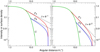Fig. 1 Profiles of the spherical and cylindrical models. Model 𝒢 has a Gaussian shape, whereas the power-law models ƤA, ƤB, ƤC, and ƤD have extended envelopes outside their Gaussian core, with the volume densities ρ ∝ r−α and intensities I ∝ θ−β (Table 1). The profiles, differing in intensity (density) by a factor of 3, fall off steeply at the outer boundary Θ = 64″ because of the adopted geometry of the finite models. The dashed profiles correspond to the “infinite” models (no outer edge within the entire image area), discussed in Sect. 4.6.

2.1 Models

Model 𝒢 has a Gaussian intensity distribution with a full width at half maximum (FWHM) of 10″ (Fig. 1). Models Ƥ_a and Ƥ_B have power-law profiles with intensities (or surface densities) I ∝ θ⁻¹ fitted to the Gaussian core, describing the cores and filaments with volume densities ρ ∝ r⁻². This choice is based on the fact that similar profiles between r^−1.5 and r^−2.5 (for large r) are expected in both the Bonnor-Ebert spheres (Bonnor 1956) and collapsing protostars (Larson 1969), as well as derived for selected young stellar objects (Sect. 4 in Men’shchikov & Henning 1997; Men’shchikov et al. 1999) and filaments (Arzoumanian et al. 2011, 2019). Models Ƥ_C and Ƥ_D with steeper profiles I ∝ θ⁻² (ρ ∝ r⁻³) are meant to test the dependence of size deconvolution results on different intensity distributions. The fitting levels of the power-law profiles, differing by a factor of 3, were chosen arbitrarily to test different contrasts of the Gaussian core with respect to the power-law wings. All models have a peak intensity of unity and an outer boundary at a radial distance r₂ from their centers, corresponding to the angular distance Θ = 64″, such that ρ = 0 for r > r₂ and I = 0 for θ > Θ. As a result of the adopted spherical and cylindrical geometries, the profiles of the power-law models fall down very steeply when θ → Θ, whereas the intensities of model 𝒢 become negligible beyond θ ≈ 20″ (Fig. 1).

It is convenient to collectively denote the power-law models as Ƥ and all five models (𝒢 and Ƥ) as ℳ. The images represent idealized sources and filaments with a high numerical resolution (small pixels), in the absence of any background or noise. To simulate the finite angular resolutions (point-spread functions or PSFs) of astronomical telescopes, the images are convolved with the circular Gaussian kernels 𝒪_j, $$\begin{array}{cc}{ℳ}_j={\mathcal{𝒪}}_j*ℳ,& j=1,2,\dots ,J\end{array},$$(1)

where J = 107 and the FWHM sizes O_j of the finely spaced set of kernels (beams, angular resolutions) between O₁ = 3.36″ and O_J = 332″ are defined as $$O_0=2^{-1/16}{O}_1,O_j=2^{1/16}{O}_{j-1},$$(2)

and the resulting images ℳ_j are renormalized to the peak intensity of the original models. The set of convolved models, computed with convolve and fftconv from the getsf source and filament extraction method¹ (Men’shchikov 2021b), simulates the entire range of the resolution states (unresolved to well resolved) of the model sources and filaments.

2.2 Backgrounds

Most extraction methods cannot disentangle the complex backgrounds from the source or filament emission and apply simple (linear) interpolation across the structures of interest, based on the pixel values just outside them (e.g., Fig. 12 in Men’shchikov et al. 2012). To investigate effects of the inaccurately determined backgrounds on the Gaussian size deconvolution, it makes sense to reduce the observed complexity and adopt only three typical shapes for the models: the flat, convex, and concave backgrounds (Fig. 2).

The flat backgrounds are assumed to always have a constant (arbitrary) value ℬ = 0.3. The two other types of backgrounds are derived, for simplicity, from the shapes of the model sources and filaments at each angular resolution, $${ℬ}_{ℳjk\pm }=ℬ\pm 0.25\left({𝒪}_{jk}*ℳ\right),$$(3)

where “+” and “−” correspond to the convex and concave backgrounds, respectively, and the FWHM sizes of the Gaussian kernels 𝒪_jk are defined by $$\begin{array}{cc}{O}_{jk}=f_k{O}_j,& k=1,2,\dots ,K,\end{array}$$(4)

where K = 9 and f_k are the background size factors, defined as $$\begin{array}{cc}{f}_0=2^{-1/8}{f}_1,& f_k\end{array}=2^{1/8}{f}_{k-1},$$(5)

in the range between 1 and 2. For f₁ = 1, the convex or concave background has the same width as that of the model at resolution O_j, whereas for f_K = 2, the background has a wider shape, corresponding to the model convolved to a twice lower resolution. With f_k > 1, the convex backgrounds tend to increase both the heights and widths of the sources, whereas the concave backgrounds contribute to their decrease.

For brevity, it is convenient to denote {𝒮|ℱ} the images of spherical or cylindrical models (Table 1, Fig. 2) and refer to either of the images as $ℐ=\left\{\mathcal{𝒮}|ℱ\right\}$. A superposition of the models and backgrounds completes the simulated images, $$\begin{array}{l}{ℐ}_{ℳj}={ℳ}_j+ℬ,\hfill \\ {ℐ}_{ℳjk\pm }={ℳ}_j+{ℬ}_{ℳjk\pm },\hfill \end{array}$$(6)

representing the idealized sources (𝒮_ℳj, 𝒮_ℳjk±) and filaments (ℱ_ℳj, ℱ_ℳjk±) with a FWHM size of 10″, blended with the three different backgrounds and observed with the wide range of angular resolutions O ≈ 3–300″. This set of images is sufficient to study effects of the complex, inaccurately subtracted backgrounds on the results of measurement and size deconvolution in real observations.

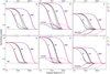Fig. 2 Profiles of the simulated sources 𝒮ℳj and 𝒮ℳjk±, defined as the convolved spherical models ℳj added to the flat, convex, and concave backgrounds (Eq. (6)). For an illustration, the profiles correspond to three angular resolutions Oj = {4,32, 256}″ (Eq. (1)) and the background size factor ƒk = 1.54 (Eq. (4)). The profiles completely overlap with each other at Oj = 256″.

2.3 Background subtraction

In this model-based study, the general, nontrivial problem of source or filament extraction in complex observed images (e.g., Men’shchikov 2021b) reduces to the separation of sources or filaments from their backgrounds and measurement of their sizes. It is assumed that the structure has been detected and its location is precisely known.

To follow the standard procedure used in the extraction methods (e.g., Sect. 3.4.6 in Men’shchikov 2021b), it is necessary to determine the source or filament footprint, defined as the image area, supposedly containing the entire emission of the structure of interest, and subtract a planar (constant) background defined by the intensity at the footprint edge. This can be accomplished by finding the angular distance Θ from the source peak or filament crest, at which the slope of intensity distribution becomes sufficiently small: $${\left|\frac{\text{d\hspace{0.17em}log\hspace{0.17em}}I\left(\theta \right)}{\text{d\hspace{0.17em}log\hspace{0.17em}}\theta }\right|}_{\text{Θ}}={10}^{-4},$$(7)

where the adopted (arbitrary) value is appropriate for the perfectly smooth model images. With this definition, the simulated (not convolved) flat-background structures I_ℳ=ℳ + ℬ have the derived footprint radii of Θ_𝒢 = 21.8″ and Θ_Ƥ = 64.09″.

The footprints expand to larger distances Θ_ℳj and Θ_ℳjk± at lower angular resolutions, when the images are convolved with increasingly larger beams O_j (Fig. 2). For models I_ℳjk− on concave backgrounds, the footprints Θ_ℳjk− correspond to the minima that develop in their intensity profiles with ƒ_k > 1, hence they become smaller than the footprints for the flat backgrounds (Fig. 2). In contrast, the models I_ℳjk+ on convex backgrounds with ƒ_k > 1 have footprints Θ_ℳjk+ that are larger than those for the flat backgrounds (Fig. 2).

When the footprints of the structures (I_ℳj·, I_ℳjk±) are determined, the background-subtracted intensity distributions, are obtained by subtracting intensities of their (interpolated) constant backgrounds, $$\begin{array}{l}{\widetilde{ℐ}}_{ℳjl}=\max \left({ℐ}_{ℳj}-\left(I\left({\text{Θ}}_{ℳj}\right)+{ϵ}_l\right),0\right),\hfill \\ {\widetilde{ℐ}}_{ℳjk\pm }=\max \left({ℐ}_{ℳjk\pm }-I\left({\text{Θ}}_{ℳjk\pm }\right),0\right),\hfill \end{array}$$(8)

where ϵ_l accounts for possible background errors, in order to test, how overestimated backgrounds affect the measured sizes and their deconvolution, $$\begin{array}{cc}{ϵ}_l=0.05\left(l-1\right),& l=1,2,\dots ,L,\end{array}$$(9)

where L = 7. The background errors ϵ_l sample values within 30% of the model maximum intensity (I(0) = 1), which is a typical range of the measurement errors for the peak intensities of faint sources, as demonstrated by source extraction benchmarks (Figs. 6–10 in Men’shchikov 2021a). Subtraction of the overestimated backgrounds I(Θ_ℳj) + ϵ_l, instead of the accurate background I(Θ_ℳj), cuts off the low-intensity pedestal of the source shape and shrinks its footprint (Fig. 3), leading to underestimated sizes, peak intensities, and integrated fluxes. It makes no sense to similarly test the underestimated backgrounds for the flat-background models, because their shapes would not change, if ϵ_l were subtracted from the background I(Θ_ℳj) in Eq. (8). The errors are applied only to the flat-background models, because the nonflat backgrounds ℬ_ℳjk± lead to under- or overestimation of the source or filament backgrounds on their own and it is important to isolate the different effects.

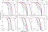Fig. 3 Proflies of the sources ${\widetilde{\mathcal{𝒮}}}_{ℳjl}$ and ${\widetilde{\mathcal{𝒮}}}_{ℳjk\pm }$ (Fig. 2), separated from the flat, convex, and concave backgrounds by subtraction of their interpolated planar backgrounds, according to Eq. (8). The profiles (solid lines) correspond to the angular resolutions Oj = {4,32, 256}″, background error ϵl = 0.05, and background size factor fk = 1.54 used in Fig. 2. The profiles completely overlap with each other at Oj = 256″. For reference, the dotted curves reproduce the true model profiles from Fig. 1. For comparison, the black dashed curves for models Ƥ{a|c} with ϵl = 0 and fk = 1 display the background-separated profiles that get almost no distortions of their shapes for Oj = 4″ in the process of background subtraction. To preserve clarity of the plots, similar profiles for models 𝒢 and Ƥ{B|D} are not shown.

2.4 Measurements

This study focuses on the measurements of half maximum sizes and their deconvolution, therefore it does not discuss measurements of other properties of extracted sources and filaments. In most algorithms, the half maximum sizes of sources are obtained assuming a Gaussian shape of their intensity distribution, by fitting two-dimensional Gaussians (e.g., in cutex, Molinari et al. 2011) or employing intensity moments (e.g., in getsources Men’shchikov et al. 2012). The sizes, estimated from the second moments of intensities (e.g., Appendix F in Men’shchikov et al. 2012), are referred to as the moment sizes in this paper.

A serious drawback of such approaches is that the assumption of Gaussian profiles is very idealized and simplistic. Various physical objects, such as the extended envelopes of protostellar cores (e.g., Larson 1969) and evolved stars (e.g., Men’shchikov et al. 2001), are well described by the power-law distributions of volume densities (ρ ∝ r⁻²) and surface densities (σ ∝ θ⁻¹), markedly different from a Gaussian. Prestellar cores, modeled as the critical Bonnor–Ebert spheres (Bonnor 1956), are also expected to have a power-law volume densities at their boundaries (ρ ∝ r^{−2 43}, Fig. 4). However, their sphericity and compactness make their surface densities appear similar to a Gaussian with a half maximum size of H_G = Θ_be above 10% of the peak, but strongly dissimilar below that level (Fig. 4).

Moreover, even an imaginary purely Gaussian structure acquires a non-Gaussian shape in the extraction process, when its background happens to be under- or overestimated, hence inaccurately subtracted (Fig. 3). As a consequence of substantial deviations of the extracted sources from a Gaussian shape, their moment sizes do not correspond to half maximum intensity. For the power-law sources Ƥ, Table 1 demonstrates that the intensity levels corresponding to their moment sizes (L_MƤ), are below the actual half maximum level by very large factors. To avoid misunderstanding and confusion, the sizes computed from the source intensity moments should not be called the FWHM sizes.

The approach of fitting a Gaussian shape to the background-subtracted source to measure its FWHM, assumes that a Gaussian shape can be found by the fitting algorithm that closely approximates the intensity distribution. Replacing the actual source shape with a fitted Gaussian gives the size estimates that do correspond to the source half maximum intensity, eliminating the problem of incompatible intensity levels of the moment sizes for different sources. A similar approach is also used to estimate the widths of filaments, when one-dimensional Gaussian is fitted to the filament profile, usually averaged along the filament length (e.g., Palmeirim et al. 2013). However, the fitting method measures properties of the fitted Gaussians, not those of the observed (non-Gaussian) sources. As a consequence, the derived half maximum sizes may be incorrect, depending on the inaccuracies of the data fitting procedure in the presence of the background and noise fluctuations and on the properties of the object that produced the observed structure shape. Fitting a Gaussian to an average filament profile ignores the important fact that filaments often have substantially different widths along their crests (e.g., Arzoumanian et al. 2019).

Both the half maximum and moment sizes are investigated in this work, following the algorithms applied by the getsf extraction method (Men’shchikov 2021b). The half maximum sizes are determined by a direct interpolation of intensity profiles (Eq. (8)) to the half maximum level (Sect. 3.4.6 in Men’shchikov 2021b), whereas the moment sizes (of sources) are computed from the second moments of intensities (Appendix F in Men’shchikov et al. 2012). The two definitions are implemented in the imgstat utility from getsf and they give identical results for the Gaussian intensity distribution (Table 1), as expected.

It is convenient to collectively denote {H|M} the true model sizes (Table 1, Fig. 1), {H|M}_j the sizes of the convolved models at a resolution O_j, and ${\left\{\tilde{H}|\tilde{M}\right\}}_j$ the sizes of the background-subtracted sources. The obvious indices ℳ, l, and k±, related to the models and backgrounds (Eq. (8)), are not given explicitly in ${\left\{\tilde{H}|\tilde{M}\right\}}_j$, to simplify the notation.

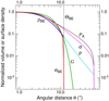Fig. 4 Profiles of the volume density ρBE (blue) and surface density σBE (red) of a critical Bonnor-Ebert sphere with an outer boundary at ΘBE = 11.9″ and a surface-density half maximum width HBE = 10″. For comparisons, the truncated ρBE continues at θ > ΘBE as ρ (cyan) and the resulting σ (magenta) corresponds to the outer boundary Θ = 64″ of the finite spherical models (Table 1). It can be easily estimated from the numerical data that the Bonnor-Ebert sphere has the power-law profiles ρ ∝ r−2.43 and σ ∝ 0−1.6 at the boundary Θ BE. For reference, the profile of model ƤA (black) is also shown.

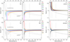Fig. 5 Deconvolution accuracy of the half maximum sizes ${\tilde{H}}_j$ for the Gaussian sources ${\widetilde{\mathcal{𝒮}}}_{𝒢jl}$ (Eq. (8)), separated from the flat background ℬ, for background over-subtraction levels 0 ≤ ϵl ≤ 0.3 (left) and from the convex and concave backgrounds ℬ𝒢jk±, for background size factors 1 ≤ ƒk ≤ 2 (right). The ratios of the deconvolved sizes Dj and Cj to the true model size H (Table 1) are plotted as functions of the model and source resolvedness Rj and ${\tilde{R}}_j$. For reference, the thin black curves display Dj/H from panels a and b and the dashed curves visualize (Oj/2)/H for ϵl = {0,0.3}. The dashed vertical lines divide the horizontal axis into the unresolved, partially resolved, and resolved domains (Eq. (11)). All curves for ϵl > 0 in panels b and d are shifted to the left in comparison with panels a and c, because the resolvedness is underestimated (${\tilde{R}}_j<R_j$). Corresponding plots for the deconvolved moment sizes ${\tilde{M}}_j$ are presented in Fig. A.1.

2.5 Resolvedness

To quantify the degree to which a source or filament is resolved (extended), it is useful to define the resolvedness R_j of the convolved model objects and the measured resolvedness ${\tilde{R}}_j$ of the background-subtracted structure, $$R_j={\left\{H|M\right\}}_j/O_j,{\tilde{R}}_j=\max \left({\left\{\tilde{H}|\tilde{M}\right\}}_j,O_j\right)/O_j.$$(10)

The model resolvedness R_j is known exclusively for the simulated models, without any background (cf. Table B.1). Only the quantity ${\tilde{R}}_j$ is available from the observed images, whose value is generally affected by the errors made in the background subtraction and size measurements. Examples of the relationships between R_j and ${\tilde{R}}_j$ for the power-law models are presented in Fig. A.3. It follows from the above definition, that only the point-like models whose smallest angular dimension fits entirely within a single pixel can have R_j = 1. All models ℳ, considered in this paper, extend over more than one pixel, therefore they have R_j > 1. Measured sizes ${\left\{\tilde{H}|\tilde{M}\right\}}_j<O_j$ would be a clear signal that they are significantly underestimated, whereas overestimated sizes do not have such obvious indicators.

It makes sense to adopt the following definitions of the state of resolvedness, based on the relationship between the beam O_j and the true object size {H|M}. When the beam is narrower than the object size, the object is considered to be resolved and when the beam is wider than twice the object size, the object is regarded as unresolved. In the intermediate range, the structure is deemed to be partially resolved. These definitions, used throughout this paper, can be summarized as $$\begin{array}{l}{\left\{R|\tilde{R}\right\}}_j>1.4\left(\text{resolved:\hspace{0.17em}}{O}_j<\left\{H|M\right\}\right),\hfill \\ 1.1<{\left\{R|\tilde{R}\right\}}_j\le 1.4\left(\text{partially:\hspace{0.17em}}\left\{H|M\right\}\le O_j<2\left\{H|M\right\}\right),\hfill \\ 1\le {\left\{R|\tilde{R}\right\}}_j\le 1.1\left(\text{unresolved: 2}\left\{H|M\right\}\le O_j\right),\hfill \end{array}$$(11)

where the limits of (5/4)^1/2 ≈ 1.1 and 2^1/2 ≈ 1.4 can be readily obtained from Eqs. (10) and (12), assuming that deconvolution recovers the true size {H|M}. In Eq. (3), the small beams (3.34″ ← O_j) are used to simulate the resolved structures (R_j → 3.14 or above), whereas the large beams (O_j → 332″) are used to simulate the unresolved sources (1 ← R_j). Examples of the resolvedness values for all models are given in Table B.1. The concept of resolvedness may be ambiguous for the structures with extended power-law profiles: there exist angular resolutions O_j, at which their interiors appear completely unresolved (2{H|M} ≪ O_j), while their extended power-law areas are well resolved (O_j ≪ 2Θ).

3 Gaussian size deconvolution

The simulated models on different backgrounds in Eq. (6) and the corresponding background-subtracted sources and filaments in Eq. (8) represent wide ranges of the observable structures, from the unresolved to the well resolved ones (Table B.1). As can be seen from Eq. (10) and Table 1, the maximum range of resolvedness in this study is 1 ≲ R₁ ≲ {H|M}Ƥ_A/O₁ ≈ {3|15}. Assuming a Gaussian shape for the source or filament intensity profile and telescope PSF, the deconvolved sizes can be conveniently derived from the basic property of convolution, $$D_j={\left({\left\{\tilde{H}|\tilde{M}\right\}}_j^2-O_j^2\right)}^{1/2},{\left\{\tilde{H}|\tilde{M}\right\}}_j\ge O_j,$$(12)

where D_j collectively denotes the deconvolved half maximum and moment sizes. For the round sources and straight filaments, convolution and deconvolution produce identical results, only when both structures have Gaussian profiles with the same width (cf. Sect. 4.6). In practice, some observational studies (e.g., Pouteau et al. 2022) use the modified (“corrected”) deconvolved sizes, $$C_j=\max \left(D_j,O_j/2\right),$$(13)

to adjust the values D_j that happened to be exceptionally small (hence considered unrealistic) to a more acceptable range. The deconvolved sizes D_j or C_j are usually interpreted in terms of the real transverse widths of the physical objects that produce the observed emission. It can be seen from Eqs. (10) and (12) that the inequalities O_j < {H|M} and O_j ≥ 2{H|M}, used in the definitions of the resolvedness domains of Eq. (11), correspond to D_j ≤ O_j/2 (or C_j > D_j) and D_j > O_j, respectively. For simplicity, next sections present results for only the half maximum sizes, whereas results for the moment sizes are described in Appendix A.

3.1 Spherical Gaussian models

The Gaussian sources 𝒮_𝒢 comply with the assumptions made in Eq. (12). The size deconvolution results for the background-subtracted sources ${\widetilde{\mathcal{𝒮}}}_{𝒢jl}$ are shown in Fig. 5. The simplest (flat) background ℬ with ϵ_l = 0 and the more complex (convex and concave) backgrounds ℬ_𝒢jk± with ƒ_k = 1 do not distort Gaussian intensity distributions, therefore they lead to accurate deconvolved sizes D_j for all angular resolutions.

Figure 5 (a, b) demonstrates that the increasingly overestimated flat backgrounds ℬ (ϵ_l > 0) lead to the progressively underestimated sizes D_j that steeply drop to zero toward the unresolved structures ($1\leftarrow {\tilde{R}}_j$), even for slightly overestimated backgrounds. In contrast, Fig. 5 (c, d) reveals that the modified deconvolved sizes C_j become greatly overestimated (more than by an order of magnitude) toward the unresolved sources ($1\leftarrow {\tilde{R}}_j$), when the background errors are small (ϵ_l → 0).

Figure 5e shows that the convex backgrounds ℬ_𝒢jk+ that happen to be wider than the sources (ƒ_k > 1) give rise to the deconvolved sizes {D|C}_j that become steeply overestimated at small ${\tilde{R}}_j$, even for the convex backgrounds that are just slightly wider than the sources. With the size factors f_k → 2, the over-estimation becomes enormously biased toward the unresolved sources, where the {D|C}_j/H curves get extremely steep on their left ends.

Figure 5f reveals that the concave backgrounds ℬ_𝒢jk− that happen to be wider than the sources (f_k > 1) result in the deconvolved sizes D_j that are substantially underestimated, steeply dropping to zero at $1\leftarrow {\tilde{R}}_j$, whereas the modified sizes C_j tend to largely compensate that deficiency at ${\tilde{R}}_j\lesssim 1.1$. However, the correction creates a bias toward overestimated sizes of the unresolved sources, while not correcting the partially resolved ones. The bias becomes strong for the backgrounds that are almost as wide as the sources (1 < f_k ≲ 1.1). When the sources are not distorted by background subtraction (f_k = 1), the sizes C_j turn out to be intolerably overestimated. For the wider backgrounds, the lower limit on D_j in Eq. (13) combines with the increasingly underestimated ${\tilde{H}}_j$ to make C_j have errors within 30–40%. Such errors might be deemed acceptable for some applications, in comparison with the overestimations in excess of an order of magnitude. In the real extractions, however, backgrounds are completely unknown and it is impossible to predict or control the actual magnitudes of the deconvolution errors.

3.2 Spherical power-law models

The power-law models 𝒮_Ƥ violate the assumptions of Eq. (12), therefore substantial errors in size deconvolution are expected. The deconvolution results for the background-subtracted power-law sources are displayed in Fig. 6. Even the simplest background ℬ with ϵ_l = 0 leads to distortions of the background-subtracted source shapes. The convex and concave backgrounds ℬ_Ƥjk±, blended with the intrinsic source shapes, alter their intensity distributions, making the background-subtracted sources wider or narrower (Fig. 3).

Larger convolution beams, used to simulate the unresolved sources ($1\leftarrow {\tilde{R}}_j$), cause greater overestimations of D_j (Fig. 6), because they incorporate more significant contributions of the power-law shapes into the source peak within its half maximum radius. Strongly overestimated deconvolved sizes D_j are obtained toward the unresolved sources, identical for all three types of backgrounds, when the background-subtracted source shapes are not distorted (ϵ_l = 0, f_k = 1). For the flat and concave backgrounds with ϵ_l > 0 and f_k > 1, the deconvolved sizes D_j turn out to be underestimated again in the limit $1\leftarrow {\tilde{R}}_j$, hence the overestimation gets localized to intermediate ranges of ${\tilde{R}}_j$ values (Fig. 6). In addition, the modified sizes C_j become steeply biased and overestimated at ${\tilde{R}}_j<1.1$.

Figure 6a demonstrates that model Ƥ_A with the most intense power-law profile on the flat background ℬ has the largest overestimation of the deconvolved sizes {D|C}_j at the lowest angular resolutions ($1\leftarrow {\tilde{R}}_j$). Subtraction of the increasingly overestimated backgrounds (ϵ_l > 0) leads to the steeper profiles (Fig. 3) and smaller {D|C}_j values, thereby somewhat compensating the errors and producing better accuracies. Model Ƥ_B, with a scaled-down power-law profile, displays a smaller over-estimation of the deconvolved sizes {D|C}_j, especially for the resolved structures (${\tilde{R}}_j\gtrsim 1.4$), because of the lesser contribution of the fainter power-law wings to the source peak (Fig. 6b). In models Ƥ_{B|C|D}, with a greater overestimation of the background (ϵ_l → 0.3), the deconvolved sizes become considerably underestimated (up to 40%), especially at the border between the partially resolved and unresolved sources (${\tilde{R}}_j\approx 1.1$).

Figure 6e demonstrates that the strongest power-law model Ƥ_A on the convex backgrounds ℬ_Ƥjk+ with f_k = 1 leads to the identical large overestimation of the deconvolved sizes {D|C}_j, like for the flat backgrounds with ϵ = 0. The wider backgrounds (f_k > 1) completely blend with the sources, widening the source peak further and causing even greater overestimation of {D|C}_j. Models Ƥ_{B|C|D} with fainter power-law profiles produce results that become more resembling those for the Gaussian sources on convex backgrounds (Fig. 5e).

Figure 6 (i–l) shows that the power-law sources 𝒮_Ƥjk− on concave backgrounds with f_k = 1 have the same large overestimation of {D|C}_j as that for the flat and convex backgrounds, because the source intensity distribution remains unchanged. The concave backgrounds that are wider than the sources (f_k > 1) lead to less overestimated or even underestimated sizes. In effect, this slightly reduces the inaccuracy of the strongly overestimated {D|C}_j. However, the errors in the modified sizes C_j remain sharply rising toward the unresolved sources ($1\leftarrow {\tilde{R}}_j$). The power-law profile is much fainter in model Ƥ_D, hence the results resemble those for the Gaussian sources in Fig. 5f.

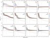Fig. 6 Deconvolution accuracy of the half maximum sizes ${\tilde{H}}_j$ for the power-law sources ${\widetilde{𝒮}}_{𝒫jl}$ and ${\widetilde{𝒮}}_{𝒫jk\pm }$ (Eq. (8)), separated from the flat (top), convex (middle), and concave (bottom) backgrounds, for background over-subtraction levels 0 ≤ ϵl ≤ 0.3 and size factors 1 ≤ fk ≤ 2. The ratio of the modified deconvolved sizes Cj to the true model size H (Table 1) is plotted as a function of the source resolvedness ${\tilde{R}}_j$. For reference, the thin black curves display Dj/H and the dashed curves visualize (Oj/2)/H for ϵl = {0,0.3} and fk = {1, 2}. Corresponding plots for the deconvolved moment sizes ${\tilde{M}}_j$ are presented in Fig. A.2.

3.3 Cylindrical Gaussian models

The Gaussian filaments ℱ_𝒢 are consistent with the assumptions made in Eq. (12). Despite their cylindrical geometry, convolution of the filaments with the Gaussian kernels O_j produces the radial profiles and sizes H_j identical to those of the equivalent sources 𝒮_𝒢 (Fig. 8). In other words, the size deconvolution results and inaccuracies for the Gaussian filaments, for all angular resolutions and background types, are identical to those presented in Sect. 3.1 (Fig. 5).

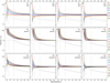Fig. 7 Deconvolution accuracy of the half maximum sizes ${\tilde{H}}_j$ for the power-law filaments ${\widetilde{ℱ}}_{𝒫jl}$ and ${\widetilde{ℱ}}_{𝒫jk\pm }$ (Eq. (8)), separated from the flat (top), convex (middle), and concave (bottom) backgrounds, for background over-subtraction levels 0 ≤ ϵl ≤ 0.3 and size factors 1 ≤ fk ≤ 2. The ratio of the modified deconvolved sizes Cj to the true model size H (Table 1) is plotted as a function of the source resolvedness ${\tilde{R}}_j$. For reference, the thin black curves display Dj/H and the dashed curves visualize (Oj/2)/H for ϵl = {0,0.3) and fk = {1, 2).

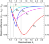Fig. 8 Dependence of the convolution results on the model geometry. Shown are the differences between the models ℳj of filaments and sources with identical radial profiles (Fig. 1), convolved with the Gaussian kernels Oj. The relative differences (HjF – HjS)/HjS of the half maximum widths of the structures are plotted as a function of the model resolvedness Rj. The corresponding deconvolution accuracies for the structures are displayed in Figs. 5–7.

3.4 Cylindrical power-law models

The power-law filaments ℱ_Ƥ are inconsistent with the assumptions made in Eq. (12). Convolution of such filaments with the Gaussian kernels creates narrower radial profiles than those of the equivalent sources 𝒮_Ƥ (Fig. 8, Sect. 4.6), depending on the model resolvedness ${\tilde{R}}_j$.

Figure 7 shows that the accuracies of the deconvolved sizes {C|D}_j for the power-law filaments, separated from the flat, convex, and concave backgrounds, are qualitatively similar to those presented in Sect. 3.2 for the power-law sources (Fig. 6). The differences between the filaments and sources for the flat background are displayed in Fig. 9. When filaments are well resolved (${\tilde{R}}_j\gg 1.4$) or unresolved ($1\leftarrow {\tilde{R}}_j<1.1$), they tend to have the same sizes as the sources, whereas in the intermediate range of $1.1\lesssim {\tilde{R}}_j\lesssim 2$ the filaments become substantially narrower than the sources. As expected, the largest differences (up to 30–40%) are found for the strongest power-law model Ƥ_A and the smallest deviations (within 10%) are shown by model Ƥ_D, resembling the Gaussian model 𝒢 most closely. Within such discrepancies, the size deconvolution results for the power-law sources 𝒮_Ƥ (Fig. 6) are also applicable to the filaments ℱ_Ƥ (Fig. 7).

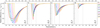Fig. 9 Comparison of the deconvolved half-maximum sizes for the power-law filaments ${\widetilde{ℱ}}_{𝒫jl}$ and sources ${\widetilde{\mathcal{𝒮}}}_{𝒫jl}$ (with identical profiles) separated from the flat background ℬ with the over-subtraction levels 0 ≤ ϵl ≤ 0.3 (Figs. 6 and 7). The relative differences between the deconvolved half maximum sizes CjF for the filaments and CjS for the sources are plotted as a function of the model resolvedness Rj. For the convex and concave backgrounds, results are qualitatively similar.

4 Discussion

4.1 Pixel sizes

This study was done using the model images with small 0.47″ pixels (Sect. 2). As a result, the convolved images that simulated the wide range of angular resolutions were progressively smoother and oversampled toward the low-resolution end, with up to 700 pixels per largest beam O_J. To verify robustness of the results (Sect. 3), the calculations were repeated with variable pixel sizes, providing the standard sampling of the astronomical images. At each angular resolution O_j, the smooth images were resampled (using swarp, Bertin et al. 2002) to always have three pixels per beam. The tests showed mostly insignificant differences with respect to the original size deconvolution results, increasing to approximately 20% for the partially resolved and unresolved structures (${\tilde{R}}_j<1.4$).

4.2 Convolution kernels

The size deconvolution results (Sect. 3), were presented for the models convolved with the Gaussian kernels 𝒪_j, which facilitated understanding and direct comparisons with the simplest reference models of the sources and filaments with Gaussian profiles. To test robustness of the results, the model objects are also convolved to the angular resolutions O_j using the kernels with the PSF shape of the Herschel SPIRE instrument at 250 µm (Aniano et al. 2011). To create such set of kernels, the PSF is resampled (using swarp) to the pixel sizes that make it correspond to the resolutions O_j.

Overall, the tests reveal minor differences, because the PSF resembles a Gaussian down to several percent of its peak (e.g., Fig. 14d). For an illustration of these results (in the case of the Gaussian model 𝒢), readers are referred to Fig. 10 (c, g, k) with practically equivalent results. The differences in D_j with respect to the original deconvolution results (Figs. 5–7) are mostly within 10% for model 𝒢 and 20% for the power-law models Ƥ. The deviations are significant only for the unresolved structures ($1\leftarrow {\tilde{R}}_j<1.1$) on the simplest backgrounds (ϵ_l = 0, f_k = 1). The deconvolved sizes D_j become steeply underestimated (D_j → 0), whereas the corrected sizes C_j are less severely overestimated than previously (by a factor of 2.5 for model 𝒢 with ϵ_l = 0). The ϵ_l > 0 and f_k > 1 cases display minor differences, because the low-level intensities, affected by the non-Gaussian PSF shape, are largely removed together with the subtracted backgrounds.

The differences are not surprising, because the PSF deviates from the Gaussian shape, violating the assumptions of the deconvolution method (Eq. (12)). As a result, the sizes become inaccurate even in the simplest case of the Gaussian model 𝒢, when the background subtraction does not modify the source shapes (ϵ_l = 0, f_k = 1), because the shape is altered by the convolution with the non-Gaussian PSF.

Additional tests with the PSF shapes of the Spitzer and Herschel instruments were done for the model of a critical Bonnor-Ebert (BE) sphere, which is often used in the studies of star formation to describe prestellar cores (Bonnor 1956). The surface densities of the critical BE sphere with a boundary radius Θ_BE are usually assumed to resemble a Gaussian with a half maximum size H_G ≈ Θ_BE (e.g., Könyves et al. 2015). The approximate similarity of the two shapes in their interiors (within 24% at θ ≈ Θ_BE/2, Fig. 4) is the consequence of the model compactness and spherical geometry. The critical BE sphere becomes, however, much steeper than a Gaussian in the outermost 10% of the sphere (0.9 Θ_BE < θ → Θ_BE), since its volume densities ρ_BE drop to zero at the outer boundary. Because of the differences and relevance for the star formation research, the size deconvolution method is tested also for the BE model using the real-life convolution kernels.

The testing is done following the standard approach, by substituting the image of the Gaussian model (Fig. 1) with that of the critical BE sphere (Fig. 4) having Θ_BE = 11.9″ and H_BE = 10″ (the same as H_ℳ, cf. Table 1). In addition to the Gaussian-shaped kernels O_j, three other sets of kernels were derived from the PSF shapes of Herschel PACS at 160 µm, Herschel SPIRE at 250 µm, and Spitzer MIPS at 160 µm (Aniano et al. 2011) by resampling them to new pixels, thereby making their half maximum widths correspond to O_j.

Figure 10 presents the deconvolution results for the critical BE model. With the Gaussian kernels, the deconvolution accuracies closely match (within 10%) those of the Gaussian model 𝒢 (Fig. 5). The realistic PSFs make the deconvolved sizes somewhat more overestimated (up to 25%) for the resolved sources. The results, shown in Fig. 10 (c, g, k), are very similar to those obtained with the SPIRE PSF for model 𝒢. Furthermore, the inaccuracies and irregularities in the D_j/H_BE curves for the unresolved sources ($1\leftarrow {\tilde{R}}_j<1.1$) increase between the four columns of panels in Fig. 10 (from left to right), along the sequence of the PSFs with progressively stronger deviations from the Gaussian shape (cf. Fig. 14 (a, d, g)). As discussed above, the BE source shape gets altered by the convolution with the non-Gaussian kernels and, therefore, the deconvolved sizes become inaccurate (D_j → 0) even in the simplest case, when the background subtraction does not modify the source shapes (ϵ_l = 0, f_k = 1).

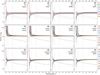Fig. 10 Deconvolution accuracy of the half maximum sizes ${\tilde{H}}_j$ for the critical Bonnor-Ebert sphere (Fig. 4), separated from the flat (top), convex (middle), and concave (bottom) backgrounds, for background over-subtraction levels 0 ≤ ϵl ≤ 0.3 and size factors 1 ≤ ƒk ≤ 2. The convolution kernels, besides a Gaussian shape, assumed the PSF shapes of Berschel PACS at 160 µm, Berschel SPIRE at 250 µm, and Spitzer MIPS at 160 µm (Aniano et al. 2011) with progressively larger deviations from the Gaussian shape. The ratio of the modified deconvolved sizes Cj to the true model size HBE = 10″ is plotted as a function of the source resolvedness ${\tilde{R}}_j$. Some curves display small irregularities in their shapes, similar to the jumps appearing in Fig. A.2, discussed in Sect. 3.2. They are also caused by the appearance of the secondary minima in the source profiles, induced by the wavy profiles of the PSFs (Fig. 14). For reference, the thin black curves display Dj/HBE and the dashed curves visualize (Oj/2)/HBE for ϵl = {0,0.3} and fk = {1,2}.

4.3 Deconvolution inaccuracies

This model-based study demonstrates that the Gaussian size deconvolution method works only when the extracted sources and filaments fully comply with the strong assumptions of Eq. (12). The deconvolved sizes D_j are accurate, when the telescope PSF is nearly Gaussian, the object that produces the observed source or filament emission has a Gaussian shape, the source or filament footprint fully includes the object’s emission, and the subtracted background is correct. The (linearly) interpolated background is accurate only when the actual background is flat. Furthermore, an accurately determined background requires that the errors caused by the noise fluctuations in the image be very low, and hence the signal-to-noise ratio for the structure must be high. Examples of the accurately deconvolved sizes D_j for all angular resolutions O_j are found in Figs. 5, A.1, and A.2, only for the simplest (unrealistic) cases (ϵ_l = 0 and f_k = 1), when the structure shape is not distorted by background subtraction.

For the simulated power-law sources 𝒮_Ƥ and filaments ℱ_Ƥ, the general trends in the deconvolution results can be understood in terms of how much their profiles (Fig. 1) deviate from the Gaussian shape 𝒢, when convolved to different angular resolutions. Models Ƥ_{A|C}, with their most intense power-law profiles, display larger inaccuracies, than do the scaled-down models Ƥ_{B|D} with smaller departures from the Gaussian model. Similarly, models Ƥ_{C|D}, with their steeper power-law profiles, resemble 𝒢 better than Ƥ_{A|B} do, hence their deconvolved sizes are less inaccurate.

The modified deconvolved sizes C_j from Eq. (13) are accurate, when all assumptions of Eq. (12) are valid and the structures are not unresolved $\left({\tilde{R}}_j\gtrsim 1.1\right)$. For the unresolved structures $\left(1\leftarrow {\tilde{R}}_j<1.1\right)$ and correctly determined backgrounds, the modified sizes C_j become greatly overestimated and steeply biased (Figs. 5–7). The great inaccuracies in C_j are especially obvious in the simplest case of the Gaussian source in Fig. 5, whose shape is not altered by background subtraction (ϵ_l = 0, f_k = 1) and for which the measured size ${\tilde{H}}_j$ is correct and the standard deconvolution of Eq. (12) gives the perfectly accurate D_j values. When deconvolution gives more accurate or even perfectly correct sizes D_j, the use of C_j is evidently counterproductive.

4.4 Background shapes

Despite the simplicity of the models of the flat, convex, and concave backgrounds, they represent three typical forms of the observed fluctuating backgrounds. The convex, concave, and more complex backgrounds totally blend with the source or filament emission and cannot be correctly deblended (interpolated). Cubic splines or even more complex interpolation schemes that one might think of are not necessarily better in practice than the simplest planar backgrounds used in the source or filament extractions. The backgrounds of the observed structures are the fundamental unknowns and unlikely to be accurately reconstructable, especially in the presence of noise and strong background fluctuations on all spatial scales. It is difficult to envision how the background values and derivatives at the edges of the structures can be determined from the data to ensure an accurate approximation of the true intensity or surface density distribution of the background cloud with cubic splines or more complex shapes. The edges of the structure footprint are poorly determined and heavily affected by the fluctuations, and the background inside the footprint remains completely unconstrained by the data.

The measured sizes and deconvolved sizes of the simulated sources and filaments do not depend on the background shape, when background subtraction does not modify the structure intensity distribution, except by just a scaling factor. The intensity shape is preserved in only two simplest cases, when the background is flat (and ϵ_l = 0) or it is convex or concave with exactly the same shape and width as the structure itself (f_k = 1). In practice, it is much more likely that subtraction of the interpolated (planar) background does alter the structure intensity distribution, which leads to very large errors in the deconvolved sizes of unresolved structures.

For the simplistic Gaussian source or filament on a flat background, even a small overestimation of the background level causes severely underestimated D_j (Fig. 5d). A similar behavior is obvious for the Gaussian structures on the concave backgrounds that happen to be wider than the structure (Fig. 5f), because the interpolated backgrounds become overestimated. In contrast, the convex backgrounds that happen to be wider than the structures, are always underestimated, which leads to the explosive overestimations of both deconvolved sizes {D|C}_j for even those structures that appear resolved (${\tilde{R}}_j\lesssim 1.2$ in Fig. 5e, and ${\tilde{R}}_j\lesssim 1.7$ in Fig. A.1).

The simulated sources and filaments with the intense power-law profiles of models Ƥ_{A|B} demonstrate a severe overestimation of the deconvolved half maximum sizes C_j, independently of the type of their background, which is worse than for the Gaussian structures (Figs. 6 and 7). At the same time, the deconvolved D_j values display strongly nonmonotonic trends to either over- or underestimations at ${\tilde{R}}_j\lesssim 1.3$ for the flat and concave backgrounds. For filaments, the amplitude of the above behavior is diminished by the fact that their convolved widths are substantially smaller than those of the sources.

The moment sizes M_j and their deconvolved values {D|C}_j are especially badly affected by the background inaccuracies, for all types of sources and backgrounds (Figs. A.1 and A.2). In general, the sizes computed from the intensity moments over the entire source footprints are too sensitive to the inaccuracies of the interpolated backgrounds, hence they are significantly less reliable than the half maximum sizes. Moreover, the intensity level, to which the moment sizes correspond, depends on the profile of the background-subtracted intensity distribution (e.g., Table 1), therefore it can strongly vary for different observed sources.

The complex observed backgrounds can only give rise to even larger inaccuracies than those reported in this paper. The wider the footprints of structures are, the less reliable the interpolated backgrounds become. Therefore, the extracted sources and filaments with strong and wide power-law wings must have less accurate backgrounds and, as a consequence, the measured and deconvolved sizes. This is consistent with a recent analysis of the Herschel filaments (André et al. 2022) that found the Gaussian size deconvolution inaccurate and unreliable for the unresolved or power-law filaments.

4.5 Physical interpretations

Interpretation of {D|C}_j in terms of the dimensions of the physical objects that produce the observed emission of sources and filaments is questionable. The deconvolved half maximum sizes, even if they were perfectly accurate, describe only the innermost bright peak, (much) smaller than the entire (footprint) diameters 2Θ of the objects (Table 1). In general, it is impossible to deduce the full extent of the partially resolved or unresolved non-Gaussian objects from the half maximum values without additional model assumptions, because of the unknown relationship between the {H|M} values and the footprints of the structures. The information is revealed in the observed images for only the well resolved sources or filaments, in which case the deconvolution loses its value, because convolution has only a minor effect on their widths.

Filaments are more difficult structures for a proper analysis than the round sources. The implicit assumptions that each physical filament lies entirely in the plane of sky and has a cylindrical geometry are unrealistic. In general, the observed filaments have substantial variations of the physical conditions (profiles, widths, linear densities, etc.) in distant segments along their crests. The usual approach to the analysis of their radial profiles and widths rests on the assumption that they have the same cylindrical properties along the entire length. With this assumption, the individual filament profiles are averaged along the entire crest (e.g., Arzoumanian et al. 2011) to dilute the background and noise fluctuations and enhance the signal-to-noise ratio of the imaginary “global” profile. An average physical property of a long and variable filament is a simplified abstract concept that needs to be replaced with the property being a function of the coordinate along its skeleton.

Most observed filaments appear significantly curved and (or) blended with a variety of other nearby structures. Convolution of a wavy filament with a telescope PSF might produce asymmetric profiles in the segments of the filament, whose radii of curvature are comparable to the angular resolution. When observed with telescope beams wider than the curvature radius of the filament segment, the latter would appear as an elongated source. Observations indicate that filament profiles are often represented by shallow power laws (e.g., Palmeirim et al. 2013; Arzoumanian et al. 2019), hence their footprints must have large and variable widths, which implies large inaccuracies in the interpolated backgrounds and profiles. With higher angular resolutions, the apparently single filaments may be expected to be resolved into thinner subfilaments (e.g., Hacar et al. 2018; Dewangan et al. 2023), like the seemingly single sources in numerical simulations are resolved into clusters (Louvet et al. 2021). Many unknowns and sources or errors can make deconvolved sizes of the filaments, extracted from observations, fairly unreliable.

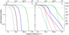Fig. 11 Convolution of the Gaussian models. The spherical (dashed curves) and cylindrical (solid curves) models 𝒢 (Fig. 1) were convolved with two types of kernels (thin dotted curves) of the half maximum sizes of {4, 32, 256}″. Shown are the results for the pure Gaussian kernels Oj (left) and power-law kernels 𝒦 j(right). The dashed horizontal lines indicate the half maximum level.

4.6 Convolution effects

There are convolution effects for different geometries of struc- tures that may be important for some studies. For an illustra- tion, it is sufficient to consider just two types of structures, represented by the round sources and straight filaments, dis- cussed in this paper. Application of the Gaussian source size deconvolution (Eq. (12)) to the filamentary geometry carries an implicit assumption that convolution always produces iden- tical profiles for the two types of the morphologically different structures. This assumption is only valid, when the source, fil- ament, and convolution kernel have perfectly Gaussian profiles and the filament crest is a straight line. Only in this simplistic case, convolution would produce the same radial profiles (and deconvolved sizes) for both sources and filaments (Fig. 11), as expected.

In the astronomical studies, it is very unlikely that the observed structures have Gaussian profiles, especially after the subtraction of an inaccurate background. Moreover, most of the observed physical objects are expected to be strongly non- Gaussian (e.g., volume density ρ ∝ r⁻², surface density σ ∝ θ⁻¹) and telescope PSFs usually have non-Gaussian, roughly power- law shapes beyond their central (Gaussian) cores. To illustrate the general behavior of convolution for different kernels, this section presents results for the Gaussian kernels O_j and sim- ple power-law kernels 𝒦_j, consisting of the Gaussian core with the half maximum size O_j and power-law wings I ∝ θ^−x with χ = 2 (Fig. 11). The simple power law, which is somewhat shal- lower and more intense than those shown by the more complex PSFs of orbital telescopes, was chosen to better illustrate the convolution effects.

The spherical and cylindrical power-law models, described in Sect. 2.1, may be referred to as the finite models, because they have an outer boundary at Θ = 64″ (Fig. 1) and there are angular resolutions O_j > 2Θ, at which the entire model becomes unresolved. It is also useful to consider the infinite models with the same power-law radial density distributions and an outer boundary, imposed by the image edge at θ = 1429″, that are resolved at all angular resolutions. The Gaussian mod- els are always finite, because their steep exponential profile has a negligible contribution at θ ≳ 20″ (Fig. 1).

Convolution of the structures of different geometry with dif- ferent kernels can seriously affect both the widths and slopes of the model profiles. The following discussion refers to the widths as the half maximum sizes (Sect. 2.4), and to the slopes, eval- uated numerically at the angular distances around θ ≈ 1000″, where all convolved power-law profiles have converged to their asymptotic behavior. Whenever the convolved models do not appear to have power-law profiles, the slopes are not computed.

4.6.1 Widths of the spherical and cylindrical models

Figure 11 demonstrates that the cylindrical Gaussian model 𝒢, convolved with the power-law kernel ’𝒦_j, is systematically wider than the equivalent spherical model. Conversely, the top panels in Fig. 12 show that the infinite cylindrical power-law models 𝒫_{A|B|C|D}*, convolved with a Gaussian kernel O_j, are systematically narrower than the equivalent spherical power-law models. However, the bottom panels in Fig. 12 reveal that the same cylindrical models, convolved with the power-law kernel 𝒦_j, are systematically wider than the spherical models, with the exception of models 𝒫_{A|B}* at the low resolutions of 32 and 256″ that become narrower than the spherical models (Fig. 12 (e, f)). The reason for the appearance of the two exceptional cases is that they are produced by the infinite models with the shallowest power-law profile, while the power-law kernel 𝒦_j is steeper than the model profile (χ > β_ℳ) and wider than the model half max- imum size (O_j ≳ H_ℳ = 10″). Apparently, the convolution in such cases with respect to the relative widths of the convolved cylindrical and spherical models behaves as if the kernel had a Gaussian shape. The transition to the exceptional cases in Fig. 12 (e, f) takes place at O_j ≈ H_M, at the border of the resolved domain (R_j ≈ 1.4, Eq. (11)). Table B.2 presents the accuracy D_j/H of the deconvolved sizes for the infinite power-law struc- tures (Fig. 12) that are especially greatly overestimated for the unresolved sources, reaching a factor of 40 at O_j = 256″.

Figure 13 reveals that the steepening of the intensity pro- file near the outer boundary at Θ = 64″ in the finite power-law models 𝒫_{A|B|C|D} makes the results of their convolution with a Gaussian kernel O_j very similar in both spherical and cylindrical geometries, the spherical model being slightly wider. However, the same cylindrical power-law models, convolved with the power-law kernel 𝒦_j, are systematically wider than the equivalent spherical model (Fig. 13), with the exception of model 𝒫_A at the resolution of 32″. The inversion with respect to the rel- ative widths of the convolved cylindrical and spherical models is confined to the range of resolutions 10 ≳ O_j ≲ 70″. The end- points of this range correspond to O_j ≈ H_ℳ and O _j ≈ Θ = 64″, where the former points to the border of the resolved domain (R_j ≈ 1.4) and the latter corresponds to the sharp drop of the profile I ∝ θ⁻¹ at the boundary of the spherical models (Fig. 1). Table B.3 presents the accuracy D_j/H of the deconvolved sizes for the finite Gaussian and power-law structures (Figs. 11 and 13) that are overestimated for the unresolved filaments up to a factor of 14 at O_j = 256″.

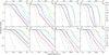Fig. 12 Convolution of the infinite power-law models (no outer edge within the entire image area). The spherical (dashed curves) and cylindrical (solid curves) models with the radial profiles, analogous to 𝒫{A|B|C|D} (Fig. 1), were convolved with two types of kernels (thin dotted curves) of the half maximum sizes of {4,32, 256}″. Shown are the results for the pure Gaussian kernels O j (top) and power-law kernels 𝒦j (bottom). The dashed horizontal lines indicate the half maximum level.

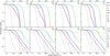Fig. 13 Convolution of the finite power-law models (with an outer edge at Θ = 64″). The spherical (dashed curves) and cylindrical (solid curves) models 𝒫{A|B|C|D} (Fig. 1) were convolved with two types of kernels (thin dotted curves) of the half maximum sizes of {4, 32, 256}″. Shown are the results for the pure Gaussian kernels Oj (top) and power-law kernels 𝒦j (bottom). The dashed horizontal lines indicate the half maximum level.

4.6.2 Slopes of the spherical and cylindrical models

Figures 11–13 reveal an effect with potential consequences for the observational studies of sources and filaments. When a con- volution kernel has substantially steeper wings than the power- law profile of the model object (χ ≥ β_ℳ + 1), the resulting slopes γ_{S|F} of the convolved sources and filaments resemble those of the true model profiles (γ_{S|F} ≈ β_ℳ), at all angular resolutions. This behavior is shown by all models after the convolution with the Gaussian kernels O_j (Fig. 12 (a–d)) and by the shallower power-law models 𝒫_{A|B} (β_ℳ = 1) after the convolution with a steeper kernel (χ = 2, Fig. 12 (e, f)).

In contrast, when the power-law wings of the kernel 𝒦_j are shallower than the profiles of the model objects (χ < β_ℳ), the convolved sources tend to resemble the kernel profile (γ_S ≈ χ), whereas the convolved filaments become signifi- cantly shallower (γ_F ≈ χ – 1). Essentially, the shallower kernel “feels” that the filament geometry has one more dimension than the source geometry, whereas the Gaussian kernel O_j is too steep to sense the differences. This behavior is displayed by the Gaussian models (Fig. 11b), Table B.3), by the infinite models 𝒫_{C|D}* (Fig. 12 (g–h), Table B.2), as well as by the finite models 𝒫_{A|B|C|A} (Fig. 13 (e–h)). Notably, the convolu- tion differences between the profiles of sources and filaments are present even when the structures are well resolved (R_j ≥ 3.4 at resolutions O_j ≤ 4″).

Convolutions of models {𝒢|𝒫_*} with the power-law kernels 𝒦_j (1.5 ≤ χ ≤ 6) confirm the geometrical differences as the general property of convolution that depends on the slopes χ of the kernel and β of the object, $${\gamma }_{\text{S}}\approx \min \left(\chi ,\beta \right),{\gamma }_{\text{F}}\approx \min \left(\chi -1,\beta \right).$$(14)

For example, when χ = β the convolved source reflects the correct slope of the object (γ_S = β), whereas the convolved fil- ament acquires a much shallower shape than that of the object (γ_F = β – 1). The kernels that are too steep with respect to the object being convolved (χ ≥ β+ 1) cannot sense the differences in geometry and, therefore, they produce the same profiles for sources and filaments, consistent with the intrinsic profile of the object (γ_S = γ_F = β).

Figure 14 displays similar convolution differences also for the Spitzer and Herschel PSFs (Aniano et al. 2011), affected by diffraction patterns, that can be approximated by somewhat steeper slopes (χ ≈ 2.8–3.1). According to Eq. (14), a filamen- tary object with an intrinsic slope β = 2, imaged by telescopes with the PSF slopes of χ ≳ 2.5, might appear as having shallower slopes in the range 1.5 ≲ γ_F ≲ 2. Convolved sources can also appear with shallower profiles, but kernels must be even shal- lower (χ < β). In other words, a spherical object observed with the above range of the PSF kernels, would always appear with the slope γ_s = 2 of the true intrinsic profile (β = 2). The convolution effects appear blurred for the PSFs with more strongly oscillat- ing profiles and steeper power-law wings. Table B.4 presents the accuracy D_j/H of the deconvolved sizes for the Gaussian and infinite power-law structures convolved with the above PSFs that end up overestimated for the unresolved sources by factors of up to 37 at O_j = 256″.

It must be noted that the above discussion assumes no back- ground or no errors in the estimated background. It is known, however, that subtraction of an inaccurate background can also seriously affect the measured slopes of the observed sources and filaments (Fig. 3).

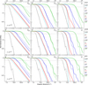Fig. 14 Convolution of the Gaussian and infinite power-law models. The spherical (dashed curves) and cylindrical (solid curves) models from Figs. 11 and 12, were convolved with two kernels (thin dotted curves) of the half maximum sizes of {4, 32, 256}″, with the PSF shapes (Aniano et al. 2011) of Herschel PACS at 70 µm (top), Herschel SPIRE at 250 µm (middle), and Spitzer MIPS at 160 µm (bottom). The black dashed lines visualize the approximate power-law slopes of the PSFs, derived by a visual fitting of their profiles over 5 orders of magnitude. The dashed horizontal lines indicate the half maximum level.

5 Conclusions

This work presents a model-based investigation of the inac- curacies and biases of the simple method of Gaussian size deconvolution (Eqs. (12) and (13)), routinely applied in many astrophysical studies to both sources and filaments extracted from observed images. Simulated images of spherical and cylin- drical objects with identical radial profiles include a Gaussian model as an idealized reference case, in addition to power-law models I ∝ θ^−β and a critical Bonnor-Ebert sphere, representing the dense cores and filaments observed in star-forming regions. To simulate observations of the model objects, the images were convolved to a wide range of angular resolutions to probe vari- ous degrees of resolvedness ${\tilde{R}}_j$ (Sect. 2.5), from the unresolved to the well-resolved structures (Eq. (11)). Three types of the model backgrounds (flat, convex, and concave), represent the simplified average shapes of fluctuating backgrounds in molecular clouds. Following the procedure used in source and filament extraction methods, planar backgrounds across the footprints of the struc- tures were interpolated and subtracted, then sizes of the sources and filaments were measured and deconvolved.

The results demonstrate that the Gaussian size deconvolution is accurate for all angular resolutions in a single simplistic case − when the telescope PSF and the background-subtracted struc- tures obey the assumption of their Gaussian shapes. In realistic situations, when background subtraction happens to be inac- curate, the extracted sources and filaments acquire profoundly non-Gaussian profiles. When the structures are unresolved ($1<{\tilde{R}}_j\le 1.1$), the deconvolved half maximum sizes can be under- or overestimated by factors of up to ∼ 20 for all models consid- ered. Both the Gaussian model (Fig. 5) and critical Bonnor-Ebert sphere (Fig. 10) display errors within a factor of ∼2 for the (par- tially) resolved structures with $1.2<{\tilde{R}}_j$ and errors of ∼ 30–20% in the resolved domain ($1.4<{\tilde{R}}_j<2$). For the resolved power- law sources and filaments (Figs. 6 and 7), the deconvolution errors can reach a factor of ∼ 6 in the worst cases, although they are generally below a factor of ∼ 2. The deconvolved moment sizes suffer from much higher errors (Figs. A.1 and A.2), com- pared to the half maximum sizes, as intensity moments are too sensitive to the inaccuracies of background subtraction.

These results demonstrate that Gaussian size deconvolution cannot be applied to unresolved structures, because of the unac- ceptably large errors. It makes sense to apply the method only to the Gaussian-like structures, including the critical Bonnor-Ebert sphere, when they are (partially) resolved (for $1.2\lesssim {\tilde{R}}_j<2$), with substantial inaccuracies of ∼50–20%. When the extracted sources or filaments have power-law intensity distributions, the range of deconvolution errors is ∼500–20% for $1.4<{\tilde{R}}_j<2$, while the deconvolution method reduces the measured sizes by only 30–13%. With the errors that are much larger than the deconvolution effect, the method must be considered inaccurate and not applicable for the power-law sources and filaments with shallow profiles (1 ← β ≲ 2).

Convolution produces identical results for different geome- tries only when both the structures and kernel have Gaussian pro- files. When convolved with a power-law kernel, the cylindrical Gaussian models are always wider than the equivalent spherical models (Fig. 11). Conversely, when convolved with a Gaus- sian kernel, the cylindrical power-law models without an outer boundary (infinite) are always narrower than the equivalent spherical models (Fig. 12). For the power-law kernels, the cylin- drical models with power-law profiles are generally wider than the equivalent spherical model, except the unresolved models with shallow profiles (β = 1), which are narrower (Fig. 12). The presence of an outer boundary in the finite power-law models makes their convolution with a Gaussian kernel similar in both spherical and cylindrical geometries (Fig. 13).

Convolution dependence on the object geometry has poten- tial consequences for the observational studies of sources and filaments, affecting even the well-resolved structures. The non- Gaussian convolution kernels (telescope PSFs) with relatively shallow power-law wings “perceive” that the filament geome- try has one more dimension than the source geometry. Such kernels can produce substantially shallower profiles for the con- volved filaments, when the kernel is shallow enough relative to the intrinsic profile of the observed object (Eq. (14)). In prin- ciple, this convolution property can cause a physical filament, imaged by the telescope with a non-Gaussian PSF with power- law wings, to appear substantially shallower than the object is in reality.

Acknowledgements

This study used the cfitsio library (Pence 1999), developed at HEASARC NASA (USA) and saoimage ds9 (Joye & Mandel 2003). The plot utility and ps 12d library, used to draw figures directly in the PostScript language, were written by the author using the psplot library (by Kevin E. Kohler), devel- oped at Nova Southeastern University Oceanographic Center (USA), and the plotting subroutines from the MHD code azeus (Ramsey et al. 2012), developed by David Clarke and the author at Saint Mary’s University (Canada). The author thanks Ph. André for useful comments and the anonymous referee for the very detailed and constructive report on the manuscript.

Appendix A Deconvolution of moment sizes

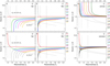Fig. A.1 Deconvolution accuracy of the moment sizes ${\tilde{M}}_j$ for the Gaussian sources ${\widetilde{\mathcal{𝒮}}}_{\mathcal{𝒢}jl}$ (Eq. (8)), separated from the flat background ℬ, for background over-subtraction levels 0 ≤ ϵl ≤ 0.3 and from the convex and concave backgrounds ℬ𝒢jk±, for background size factors 1 ≤ ƒk ≤ 2 (right). The ratios of the deconvolved sizes Dj and Cj to the true model size M (Table 1) are plotted as functions of the model and source resolvedness Rj and ${\tilde{R}}_j$. For reference, the thin black curves display Dj/M from panels a and b and the dashed curves visualize (Oj/2)/M for ϵl = {0, 0.3}. The dashed vertical lines divide the horizontal axis into the unresolved, partially resolved, and resolved domains (Eq. (11)). All curves for ϵl > 0 in panels b and d are shifted to the left in comparison with panels a and c because the resolvedness is underestimated (${\tilde{R}}_j>R_j$). The deconvolution errors in panel e for the convex case with ƒk ≥ 1.54 reach the values of 24, 29, 34, and 41. Corresponding plots for the deconvolved half maximum sizes ${\tilde{H}}_j$ are presented in Fig. 5.

Appendix A.1 Spherical Gaussian models

The deconvolved moment sizes for the Gaussian sources ${\widetilde{𝒮}}_{𝒢jl}$ on the flat backgrounds ℬ are shown in Fig. A.1 (a–d). Although the accuracy curves are qualitatively similar to those presented in Fig. 5 (a–d) for the half maximum sizes, the deconvolution errors become larger by a factor of two at R_j > 1.1. For the overesti- mated backgrounds with ϵ_l > 0, the moment sizes {D|C}_j always become more underestimated, because the intensity moments depend on the outer parts of the intensity distribution that are more distorted by background subtraction (Fig. 3).

The deconvolved moment sizes for the Gaussian sources ${\widetilde{𝒮}}_{𝒢jl}$ on the convex and concave backgrounds ℬ_𝒢jk± are presented in Fig. A.1 (e,f). The resulting accuracies behave qualitatively sim- ilar to the ones shown in Fig. 5 (e, f) for the half maximum sizes, although with larger errors. For the wider convex backgrounds (with ƒ_k > 1), the deconvolved moment sizes {D|C}_j are strongly overestimated (by factors of 17–41) within R_j ≲ 1.7 (Fig. A.1 (e)), that is even for the resolved sources. In contrast, the over- estimation of the half maximum sizes (by a factor of 17) was limited to R_j ≲ 1.2 (Fig. 5 (e)). This is because the faint out- skirts of the Gaussian sources are much more affected by the blending with the wider hill-like backgrounds than their peaks around half maximum. For the concave backgrounds with ƒk > 1, the moment sizes D_j are underestimated by 50% at R_j = 1.1 (Fig. A.1 (f)), in contrast to 30% for the half maximum sizes (Fig. 5 (f)). At the same time, the moment sizes C_j remain strongly biased toward the unresolved sources ($1\leftarrow {\tilde{R}}_j\lesssim 1.1$).

Appendix A.2 Spherical power-law models

The deconvolved moment sizes for the power-law sources are markedly different from the half maximum sizes, because the intensity moments get a major contribution from the extended power-law profiles (cf. Table 1). The simple background ℬ enables its precise subtraction (with ϵ_l = 0) and accurate deconvolution for the moment sizes D_j (Fig. A.2). For the convex and concave backgrounds that do not distort the source shapes (ƒ_k = 1), the deconvolved moment sizes D_j are also perfectly accurate. In these simplest cases, the modified sizes C_j become steeply overestimated for the unresolved sources ($1\leftarrow {\tilde{R}}_j<1.1$). For the three types of backgrounds, reduction in the strength of the power-law profiles of 𝒫_B, 𝒫_C, and 𝒫_D, progressively worsens the deconvolution results for the moment sizes {D|C}_j (Fig. A.2), in contrast to those for the half maximum sizes (Fig. 6). This is because subtraction of an overestimated background makes the source profiles steepen (drop to zero) toward the outer boundary (Fig. 3).

For the power-law models 𝒫_{a|b|C|d} on the flat background ℬ that happen to be over-subtracted (ϵ_l > 0), the deconvolved moment sizes {D|C}_j become severely underestimated (Fig. A.2 (a–d)). For the wider convex backgrounds ℬ_𝒫jk+ (with ƒ_k > 1), the moment sizes are steeply overestimated (Fig. A.2 (e–h)), even for the resolved sources at $1.4\lesssim {\tilde{R}}_j\lesssim 1.7$, which is qual- itatively similar to the Gaussian sources (Fig. A.1 (e)). For the wider concave backgrounds ℬ_𝒫jk−, the deconvolved moment sizes become more underestimated (Fig. A.2 (i–l)) than for the Gaussian sources (Fig. A.1 (f)). For certain angular resolutions Oj and factors f_k, models 𝒫{B|C|D} exhibit discontinuous jumps in the D_j and ${\tilde{R}}_j$ values between j and j + 1 (Fig. A.2) (j–l). The jumps are caused by the sudden changes of the footprint radii Θ_ℳjk− triggered by the footprint determination algorithm of Eq. (7) in the perfectly smooth model images of sources and backgrounds.

Fig. A.2 Deconvolution accuracy of the moment sizes ${\tilde{M}}_j$ for the power-law sources ${\widetilde{𝒮}}_{𝒫jl}$ and ${\widetilde{𝒮}}_{𝒫jk\pm }$ (Eq. (8)), separated from the flat (top), convex (middle), and concave (bottom) backgrounds, for background over-subtraction levels 0 ≤ ϵl ≤ 0.3 and size factors 1 ≤ fk ≤ 2. The ratio of the modified deconvolved sizes Cj to the true model size M (Table 1) is plotted as a function of the source resolvedness ${\tilde{R}}_j$. The dashed curves indicate discontinuous jumps in ${\tilde{R}}_j$ between j and j + 1 (at certain Oj values), caused by the jumps in the footprint radii Θℳjk- (Eq. (7)) and sizes ${\tilde{M}}_j$ (cf. Fig. A.3). For reference, the thin black curves display Dj/M and the dashed curves visualize (Oj/2)/M for ϵl = {0, 0.3} and fk = {1, 2}. Corresponding plots for the deconvolved half maximum sizes ${\tilde{H}}_j$ are presented in Fig. 6.

The footprint changes in Fig. A.2 (j–l) are caused by the appearance or disappearance of a shallow secondary intensity minimum in the source shape, when it is superposed on the concave background (Fig. 2). The profiles of some power-law models become fairly flat over a wide range of 9 (best visible in 𝒫_{B|D} at O_j = 4″), which leads to the appearance of the secondary minima for some combinations of the model profile (Fig. 1), angular resolutions (Eq. (1)), and background shapes (Eq. (3)). The sudden footprint changes lead to substantial varia- tions in the background-subtracted intensity distributions, hence in the moment sizes ${\tilde{M}}_j$ and resolvedness ${\tilde{R}}_j$. To clarify the deconvolution results presented in this paper, as well as the rea- sons behind the jumps, the relationships between R_j and ${\tilde{R}}_j$ for the power-law models are shown in Fig. A.3.

Source extractions in observed images do not show such sub- tle effects, because the shallow minima in the low-intensity areas are destroyed by the noise and background fluctuations. The jumpy curves in Fig. A.2 are to be ignored, because the decon- volution (in)accuracy for the moment sizes, associated with the concave backgrounds, is clearly demonstrated by the continuous curves.

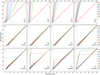Fig. A.3 Relationships between the model resolvedness Rj and ${\tilde{R}}_j$ (Sect. 2.5, Eq. (10)) for the results presented in Fig. A.2. The plots (with wide ranges of resolvedness values) are useful for a better comprehension of the deconvolution accuracy plots in Figs. 5–7, 10, A.1, and A.2, as well as the discontinuous jumps in Fig. A.2 (j−l).

Appendix B Tabulated material

Table B.1 presents the values for the model resolvedness R_j (Sect. 2.5), corresponding to the half maximum and moment sizes at selected angular resolutions O_j. Tables B.2, B.3, and B.4 present the deconvolution accuracies and power-law slopes, corresponding to the convolved infinite and finite models in Figs. 12, 13, and 14 (Sect. 4.6).

References

All Tables

All Figures

Fig. 1 Profiles of the spherical and cylindrical models. Model 𝒢 has a Gaussian shape, whereas the power-law models ƤA, ƤB, ƤC, and ƤD have extended envelopes outside their Gaussian core, with the volume densities ρ ∝ r−α and intensities I ∝ θ−β (Table 1). The profiles, differing in intensity (density) by a factor of 3, fall off steeply at the outer boundary Θ = 64″ because of the adopted geometry of the finite models. The dashed profiles correspond to the “infinite” models (no outer edge within the entire image area), discussed in Sect. 4.6.

In the text

	Fig. 2 Profiles of the simulated sources 𝒮ℳj and 𝒮ℳjk±, defined as the convolved spherical models ℳj added to the flat, convex, and concave backgrounds (Eq. (6)). For an illustration, the profiles correspond to three angular resolutions Oj = {4,32, 256}″ (Eq. (1)) and the background size factor ƒk = 1.54 (Eq. (4)). The profiles completely overlap with each other at Oj = 256″.
In the text

Fig. 3 Proflies of the sources ${\widetilde{\mathcal{𝒮}}}_{ℳjl}$ and ${\widetilde{\mathcal{𝒮}}}_{ℳjk\pm }$ (Fig. 2), separated from the flat, convex, and concave backgrounds by subtraction of their interpolated planar backgrounds, according to Eq. (8). The profiles (solid lines) correspond to the angular resolutions Oj = {4,32, 256}″, background error ϵl = 0.05, and background size factor fk = 1.54 used in Fig. 2. The profiles completely overlap with each other at Oj = 256″. For reference, the dotted curves reproduce the true model profiles from Fig. 1. For comparison, the black dashed curves for models Ƥ{a|c} with ϵl = 0 and fk = 1 display the background-separated profiles that get almost no distortions of their shapes for Oj = 4″ in the process of background subtraction. To preserve clarity of the plots, similar profiles for models 𝒢 and Ƥ{B|D} are not shown.

In the text

Fig. 4 Profiles of the volume density ρBE (blue) and surface density σBE (red) of a critical Bonnor-Ebert sphere with an outer boundary at ΘBE = 11.9″ and a surface-density half maximum width HBE = 10″. For comparisons, the truncated ρBE continues at θ > ΘBE as ρ (cyan) and the resulting σ (magenta) corresponds to the outer boundary Θ = 64″ of the finite spherical models (Table 1). It can be easily estimated from the numerical data that the Bonnor-Ebert sphere has the power-law profiles ρ ∝ r−2.43 and σ ∝ 0−1.6 at the boundary Θ BE. For reference, the profile of model ƤA (black) is also shown.

In the text

Fig. 5 Deconvolution accuracy of the half maximum sizes ${\tilde{H}}_j$ for the Gaussian sources ${\widetilde{\mathcal{𝒮}}}_{𝒢jl}$ (Eq. (8)), separated from the flat background ℬ, for background over-subtraction levels 0 ≤ ϵl ≤ 0.3 (left) and from the convex and concave backgrounds ℬ𝒢jk±, for background size factors 1 ≤ ƒk ≤ 2 (right). The ratios of the deconvolved sizes Dj and Cj to the true model size H (Table 1) are plotted as functions of the model and source resolvedness Rj and ${\tilde{R}}_j$. For reference, the thin black curves display Dj/H from panels a and b and the dashed curves visualize (Oj/2)/H for ϵl = {0,0.3}. The dashed vertical lines divide the horizontal axis into the unresolved, partially resolved, and resolved domains (Eq. (11)). All curves for ϵl > 0 in panels b and d are shifted to the left in comparison with panels a and c, because the resolvedness is underestimated (${\tilde{R}}_j<R_j$). Corresponding plots for the deconvolved moment sizes ${\tilde{M}}_j$ are presented in Fig. A.1.

In the text

Fig. 6 Deconvolution accuracy of the half maximum sizes ${\tilde{H}}_j$ for the power-law sources ${\widetilde{𝒮}}_{𝒫jl}$ and ${\widetilde{𝒮}}_{𝒫jk\pm }$ (Eq. (8)), separated from the flat (top), convex (middle), and concave (bottom) backgrounds, for background over-subtraction levels 0 ≤ ϵl ≤ 0.3 and size factors 1 ≤ fk ≤ 2. The ratio of the modified deconvolved sizes Cj to the true model size H (Table 1) is plotted as a function of the source resolvedness ${\tilde{R}}_j$. For reference, the thin black curves display Dj/H and the dashed curves visualize (Oj/2)/H for ϵl = {0,0.3} and fk = {1, 2}. Corresponding plots for the deconvolved moment sizes ${\tilde{M}}_j$ are presented in Fig. A.2.

In the text

Fig. 7 Deconvolution accuracy of the half maximum sizes ${\tilde{H}}_j$ for the power-law filaments ${\widetilde{ℱ}}_{𝒫jl}$ and ${\widetilde{ℱ}}_{𝒫jk\pm }$ (Eq. (8)), separated from the flat (top), convex (middle), and concave (bottom) backgrounds, for background over-subtraction levels 0 ≤ ϵl ≤ 0.3 and size factors 1 ≤ fk ≤ 2. The ratio of the modified deconvolved sizes Cj to the true model size H (Table 1) is plotted as a function of the source resolvedness ${\tilde{R}}_j$. For reference, the thin black curves display Dj/H and the dashed curves visualize (Oj/2)/H for ϵl = {0,0.3) and fk = {1, 2).

In the text

Fig. 8 Dependence of the convolution results on the model geometry. Shown are the differences between the models ℳj of filaments and sources with identical radial profiles (Fig. 1), convolved with the Gaussian kernels Oj. The relative differences (HjF – HjS)/HjS of the half maximum widths of the structures are plotted as a function of the model resolvedness Rj. The corresponding deconvolution accuracies for the structures are displayed in Figs. 5–7.

In the text

Fig. 9 Comparison of the deconvolved half-maximum sizes for the power-law filaments ${\widetilde{ℱ}}_{𝒫jl}$ and sources ${\widetilde{\mathcal{𝒮}}}_{𝒫jl}$ (with identical profiles) separated from the flat background ℬ with the over-subtraction levels 0 ≤ ϵl ≤ 0.3 (Figs. 6 and 7). The relative differences between the deconvolved half maximum sizes CjF for the filaments and CjS for the sources are plotted as a function of the model resolvedness Rj. For the convex and concave backgrounds, results are qualitatively similar.

In the text

Fig. 10 Deconvolution accuracy of the half maximum sizes ${\tilde{H}}_j$ for the critical Bonnor-Ebert sphere (Fig. 4), separated from the flat (top), convex (middle), and concave (bottom) backgrounds, for background over-subtraction levels 0 ≤ ϵl ≤ 0.3 and size factors 1 ≤ ƒk ≤ 2. The convolution kernels, besides a Gaussian shape, assumed the PSF shapes of Berschel PACS at 160 µm, Berschel SPIRE at 250 µm, and Spitzer MIPS at 160 µm (Aniano et al. 2011) with progressively larger deviations from the Gaussian shape. The ratio of the modified deconvolved sizes Cj to the true model size HBE = 10″ is plotted as a function of the source resolvedness ${\tilde{R}}_j$. Some curves display small irregularities in their shapes, similar to the jumps appearing in Fig. A.2, discussed in Sect. 3.2. They are also caused by the appearance of the secondary minima in the source profiles, induced by the wavy profiles of the PSFs (Fig. 14). For reference, the thin black curves display Dj/HBE and the dashed curves visualize (Oj/2)/HBE for ϵl = {0,0.3} and fk = {1,2}.

In the text

	Fig. 11 Convolution of the Gaussian models. The spherical (dashed curves) and cylindrical (solid curves) models 𝒢 (Fig. 1) were convolved with two types of kernels (thin dotted curves) of the half maximum sizes of {4, 32, 256}″. Shown are the results for the pure Gaussian kernels Oj (left) and power-law kernels 𝒦 j(right). The dashed horizontal lines indicate the half maximum level.
In the text

Fig. 12 Convolution of the infinite power-law models (no outer edge within the entire image area). The spherical (dashed curves) and cylindrical (solid curves) models with the radial profiles, analogous to 𝒫{A|B|C|D} (Fig. 1), were convolved with two types of kernels (thin dotted curves) of the half maximum sizes of {4,32, 256}″. Shown are the results for the pure Gaussian kernels O j (top) and power-law kernels 𝒦j (bottom). The dashed horizontal lines indicate the half maximum level.

In the text

Fig. 13 Convolution of the finite power-law models (with an outer edge at Θ = 64″). The spherical (dashed curves) and cylindrical (solid curves) models 𝒫{A|B|C|D} (Fig. 1) were convolved with two types of kernels (thin dotted curves) of the half maximum sizes of {4, 32, 256}″. Shown are the results for the pure Gaussian kernels Oj (top) and power-law kernels 𝒦j (bottom). The dashed horizontal lines indicate the half maximum level.

In the text

Fig. 14 Convolution of the Gaussian and infinite power-law models. The spherical (dashed curves) and cylindrical (solid curves) models from Figs. 11 and 12, were convolved with two kernels (thin dotted curves) of the half maximum sizes of {4, 32, 256}″, with the PSF shapes (Aniano et al. 2011) of Herschel PACS at 70 µm (top), Herschel SPIRE at 250 µm (middle), and Spitzer MIPS at 160 µm (bottom). The black dashed lines visualize the approximate power-law slopes of the PSFs, derived by a visual fitting of their profiles over 5 orders of magnitude. The dashed horizontal lines indicate the half maximum level.

In the text

Fig. A.1 Deconvolution accuracy of the moment sizes ${\tilde{M}}_j$ for the Gaussian sources ${\widetilde{\mathcal{𝒮}}}_{\mathcal{𝒢}jl}$ (Eq. (8)), separated from the flat background ℬ, for background over-subtraction levels 0 ≤ ϵl ≤ 0.3 and from the convex and concave backgrounds ℬ𝒢jk±, for background size factors 1 ≤ ƒk ≤ 2 (right). The ratios of the deconvolved sizes Dj and Cj to the true model size M (Table 1) are plotted as functions of the model and source resolvedness Rj and ${\tilde{R}}_j$. For reference, the thin black curves display Dj/M from panels a and b and the dashed curves visualize (Oj/2)/M for ϵl = {0, 0.3}. The dashed vertical lines divide the horizontal axis into the unresolved, partially resolved, and resolved domains (Eq. (11)). All curves for ϵl > 0 in panels b and d are shifted to the left in comparison with panels a and c because the resolvedness is underestimated (${\tilde{R}}_j>R_j$). The deconvolution errors in panel e for the convex case with ƒk ≥ 1.54 reach the values of 24, 29, 34, and 41. Corresponding plots for the deconvolved half maximum sizes ${\tilde{H}}_j$ are presented in Fig. 5.

In the text

Fig. A.2 Deconvolution accuracy of the moment sizes ${\tilde{M}}_j$ for the power-law sources ${\widetilde{𝒮}}_{𝒫jl}$ and ${\widetilde{𝒮}}_{𝒫jk\pm }$ (Eq. (8)), separated from the flat (top), convex (middle), and concave (bottom) backgrounds, for background over-subtraction levels 0 ≤ ϵl ≤ 0.3 and size factors 1 ≤ fk ≤ 2. The ratio of the modified deconvolved sizes Cj to the true model size M (Table 1) is plotted as a function of the source resolvedness ${\tilde{R}}_j$. The dashed curves indicate discontinuous jumps in ${\tilde{R}}_j$ between j and j + 1 (at certain Oj values), caused by the jumps in the footprint radii Θℳjk- (Eq. (7)) and sizes ${\tilde{M}}_j$ (cf. Fig. A.3). For reference, the thin black curves display Dj/M and the dashed curves visualize (Oj/2)/M for ϵl = {0, 0.3} and fk = {1, 2}. Corresponding plots for the deconvolved half maximum sizes ${\tilde{H}}_j$ are presented in Fig. 6.

In the text

	Fig. A.3 Relationships between the model resolvedness Rj and ${\tilde{R}}_j$ (Sect. 2.5, Eq. (10)) for the results presented in Fig. A.2. The plots (with wide ranges of resolvedness values) are useful for a better comprehension of the deconvolution accuracy plots in Figs. 5–7, 10, A.1, and A.2, as well as the discontinuous jumps in Fig. A.2 (j−l).
In the text

References

- André, P., Revéret, V., Könyves, V., et al. 2016, A&A, 592, A54 [NASA ADS] [CrossRef] [EDP Sciences] [Google Scholar]
- André, P., Palmeirim, P., & Arzoumanian, D. 2022, A&A, 667, A1 [Google Scholar]
- Aniano, G., Draine, B. T., Gordon, K. D., & Sandstrom, K. 2011, PASP, 123, 1218 [Google Scholar]
- Arzoumanian, D., André, P., Didelon, P., et al. 2011, A&A, 529, A6 [Google Scholar]
- Arzoumanian, D., André, P., Könyves, V., et al. 2019, A&A, 621, A42 [NASA ADS] [CrossRef] [EDP Sciences] [Google Scholar]
- Bertin, E., Mellier, Y., Radovich, M., et al. 2002, ASP Conf. Ser., 281, 228 [Google Scholar]
- Bonnor, W. B. 1956, MNRAS, 116, 351 [NASA ADS] [CrossRef] [Google Scholar]
- Bontemps, S., Motte, F., Csengeri, T., & Schneider, N. 2010, A&A, 524, A18 [NASA ADS] [CrossRef] [EDP Sciences] [Google Scholar]
- Cox, N. L. J., Arzoumanian, D., André, P., et al. 2016, A&A, 590, A110 [NASA ADS] [CrossRef] [EDP Sciences] [Google Scholar]
- Dewangan, L. K., Bhadari, N. K., Men’shchikov, A., et al. 2023, ApJ, 946, 22 [NASA ADS] [CrossRef] [Google Scholar]
- Hacar, A., Tafalla, M., Forbrich, J., et al. 2018, A&A, 610, A77 [NASA ADS] [CrossRef] [EDP Sciences] [Google Scholar]
- Joye, W. A., & Mandel, E. 2003, ASP Conf. Ser., 295, 489 [Google Scholar]
- Könyves, V., André, P., Men’shchikov, A., et al. 2015, A&A, 584, A91 [Google Scholar]
- Ladjelate, B., André, P., Könyves, V., et al. 2020, A&A, 638, A74 [NASA ADS] [CrossRef] [EDP Sciences] [Google Scholar]
- Larson, R. B. 1969, MNRAS, 145, 271 [Google Scholar]
- Louvet, F., Hennebelle, P., Men’shchikov, A., et al. 2021, A&A, 653, A157 [NASA ADS] [CrossRef] [EDP Sciences] [Google Scholar]
- Men’shchikov, A. 2021a, A&A, 654, A78 [NASA ADS] [CrossRef] [EDP Sciences] [Google Scholar]
- Men’shchikov, A. 2021b, A&A, 649, A89 [EDP Sciences] [Google Scholar]
- Men’shchikov, A. B., & Henning, T. 1997, A&A, 318, 879 [Google Scholar]
- Men’shchikov, A. B., Henning, T., & Fischer, O. 1999, ApJ, 519, 257 [CrossRef] [Google Scholar]
- Men’shchikov, A. B., Balega, Y., Blöcker, T., Osterbart, R., & Weigelt, G. 2001, A&A, 368, 497 [NASA ADS] [CrossRef] [EDP Sciences] [Google Scholar]
- Men’shchikov, A., André, P., Didelon, P., et al. 2012, A&A, 542, A81 [Google Scholar]
- Molinari, S., Schisano, E., Faustini, F., et al. 2011, A&A, 530, A133 [NASA ADS] [CrossRef] [EDP Sciences] [Google Scholar]
- Motte, F., Schilke, P., & Lis, D. C. 2003, ApJ, 582, 277 [NASA ADS] [CrossRef] [Google Scholar]
- Nguyen Luong, Q., Motte, F., Hennemann, M., et al. 2011, A&A, 535, A76 [NASA ADS] [CrossRef] [EDP Sciences] [Google Scholar]
- Padoan, P., Pelkonen, V. M., Juvela, M., Haugbølle, T., & Nordlund, Å. 2023, MNRAS, 522, 3548 [NASA ADS] [CrossRef] [Google Scholar]
- Palmeirim, P., André, P., Kirk, J., et al. 2013, A&A, 550, A38 [NASA ADS] [CrossRef] [EDP Sciences] [Google Scholar]
- Pence, W. 1999, ASP Conf. Ser., 172, 487 [NASA ADS] [Google Scholar]
- Pouteau, Y., Motte, F., Nony, T., et al. 2022, A&A, 664, A26 [NASA ADS] [CrossRef] [EDP Sciences] [Google Scholar]
- Ramsey, J. P., Clarke, D. A., & Men’shchikov, A. B. 2012, ApJS, 199, 13 [Google Scholar]
All Tables
Deconvolution accuracy ratios A = Dj/H (left) and power-law slopes γ (right) for the infinite power-law sources 𝒮 and filaments ℱ (Sect. 4.6) with profiles, analogous to 𝒫{A|B|C|D} (Fig. 1), convolved with the Gaussian kernels 𝒪j and power-law kernels 𝒦j of half maximum sizes Oj (cf. Fig. 12), without any background.
Deconvolution accuracy ratios A = Dj/H (left) and power-law slopes γ (right) for the finite Gaussian and power-law sources 𝒮 and filaments ℱ (Sect. 4.6) with profiles {𝒢|𝒫{A|B|C|D}} from Fig. 1, convolved with the Gaussian kernels 𝒪j and power-law kernels 𝒦j· of half maximum sizes Oj (cf. Fig. 13), without any background. These results correspond to those presented in Sect. 3 for a perfectly subtracted flat background (∈l = 0).
Deconvolution accuracy ratios A = Dj/H for the Gaussian and infinite power-law sources S and filaments ℱ (Sect. 4.6) with profiles, analogous to {𝒢|𝒫{A|C}} from Fig. 1, convolved with kernels with the PSF shapes (Aniano et al. 2011) of Berschel PACS at 70 µm, Berschel SPIRE at 250 µm, and Spitzer MIPS at 160 µm (the kernel profiles are shown in Fig. 14).