| Issue |
A&A
Volume 667, November 2022
|
|
|---|---|---|
| Article Number | L1 | |
| Number of page(s) | 8 | |
| Section | Letters to the Editor | |
| DOI | https://doi.org/10.1051/0004-6361/202244541 | |
| Published online | 28 October 2022 | |
Letter to the Editor
The typical width of Herschel filaments
1
Laboratoire d’Astrophysique (AIM), Université Paris-Saclay, Université Paris Cité, CEA, CNRS, AIM, 91191 Gif-sur-Yvette, France
e-mail: This email address is being protected from spambots. You need JavaScript enabled to view it.
2
Instituto de Astrofísica e Ciências do Espaço, Universidade do Porto, CAUP, Rua das Estrelas, 4150-762 Porto, Portugal
e-mail: This email address is being protected from spambots. You need JavaScript enabled to view it.
3
National Astronomical Observatory of Japan, Osawa 2-21-1, Mitaka, Tokyo 181-8588, Japan
e-mail: This email address is being protected from spambots. You need JavaScript enabled to view it.
Received:
19
July
2022
Accepted:
10
October
2022
Abstract
Context. Dense molecular filaments are widely believed to be representative of the initial conditions of star formation in interstellar clouds. Characterizing their physical properties, such as their transverse size, is therefore of paramount importance. Herschel studies suggest that nearby (d < 500 pc) molecular filaments have a typical half-power width of ∼0.1 pc, but this finding has been questioned recently on the ground that the measured widths tend to increase with distance to the filaments.
Aims. Here we revisit the dependence of measured filament widths on distance or, equivalently, spatial resolution in an effort to determine whether nearby molecular filaments have a characteristic half-power width or whether this is an artifact of the finite resolution of the Herschel data.
Methods. We perform a convergence test on the well-documented B211/213 filament in Taurus by degrading the resolution of the Herschel data several times and reestimating the filament width from the resulting column density profiles. We also compare the widths measured for the Taurus filament and other filaments from the Herschel Gould Belt Survey to those found for synthetic filaments with various types of simple, idealized column density profiles (Gaussian, power law, and Plummer-like).
Results. We find that the measured filament widths do increase slightly as the spatial resolution worsens and/or the distance to the filaments increases. However, this trend is entirely consistent with what is expected from simple beam convolution for filaments with density profiles that are Plummer-like and have intrinsic half-power diameters of ∼0.08–0.1 pc and logarithmic slopes 1.5 < p < 2.5 at large radii, as directly observed in many cases, including for the Taurus filament. Due to the presence of background noise fluctuations, deconvolution of the measured widths from the telescope beam is difficult and quickly becomes inaccurate.
Conclusions. We conclude that the typical half-power filament width of ∼0.1 pc measured with Herschel in nearby clouds most likely reflects the presence of a true common scale in the filamentary structure of the cold interstellar medium, at least in the solar neighborhood. We suggest that this common scale may correspond to the magnetized turbulent correlation length in molecular clouds.
Key words: stars: formation / ISM: clouds / ISM: structure / submillimeter: ISM
© P. J. André et al. 2022
 Open Access article, published by EDP Sciences, under the terms of the Creative Commons Attribution License (https://creativecommons.org/licenses/by/4.0), which permits unrestricted use, distribution, and reproduction in any medium, provided the original work is properly cited.
This article is published in open access under the Subscribe-to-Open model. This email address is being protected from spambots. You need JavaScript enabled to view it. to support open access publication.
1. Introduction
The filamentary texture of the cold interstellar medium is believed to play a central role in the star formation process (e.g., Hacar et al. 2022; Pineda et al. 2022, for recent reviews). In particular, Herschel imaging surveys of nearby Galactic clouds (André et al. 2010; Molinari et al. 2010; Hill et al. 2011; Juvela et al. 2012) have shown that filaments dominate the mass budget of molecular clouds at high densities (e.g., Schisano et al. 2014) and correspond to the birthplaces of most prestellar cores (e.g., Könyves et al. 2015; Marsh et al. 2016; Di Francesco et al. 2020). These findings support the notion that molecular filaments are representative of the initial conditions of the bulk of star formation in the Galaxy (e.g., André et al. 2014). Characterizing their detailed physical properties is therefore of paramount importance. A key attribute of filamentary gas structures is their transverse diameter since the fragmentation properties of cylindrical filaments are expected to scale with the filament diameter, at least according to quasi-static fragmentation models (e.g., Nagasawa 1987; Inutsuka & Miyama 1992). Remarkably, Herschel observations suggest that nearby molecular filaments have a common width of ∼0.1 pc, with some scatter around this value (Arzoumanian et al. 2011, 2019). Indeed, analyzing the radial column density profiles of 599 Herschel filaments in eight nearby clouds at d < 500 pc, Arzoumanian et al. (2019) found that the filaments of their sample share approximately the same half-power (HP) width, ∼0.1 pc with a spread of a factor of ∼2, regardless of their mass per unit length, Mline, and whether they are subcritical with Mline ≲ 0.5 Mline, crit, transcritical with 0.5 Mline, crit ≲ Mline ≲ 2 Mline, crit, or thermally supercritical with Mline ≳ 2 Mline, crit. Here,  is the thermal value of the critical mass per unit length (e.g., Ostriker 1964), which is ∼16 M⊙ pc−1 for a sound speed cs ∼ 0.2 km s−1 or a gas temperature T ≈ 10 K. If confirmed, the existence of a typical filament width may have far-reaching implications as it introduces a characteristic length scale, and possibly a characteristic mass scale as well (André et al. 2019), in the structure of molecular clouds, which is believed to be hierarchical in nature and essentially scale-free.
However, the reliability of the filament widths derived from Herschel data has recently been questioned by Panopoulou et al. (2022), who report an intriguing correlation between the measured widths and the distances of the Herschel filaments in the Arzoumanian et al. (2019) sample. Panopoulou et al. (2022) suggest that the filament widths derived by Arzoumanian et al. (2019) are strongly affected by the finite spatial resolution of the Herschel data and inconsistent with a characteristic intrinsic filament diameter of ∼0.1 pc.
In this paper we reexamine the effect of spatial resolution on the column density profiles derived from Herschel data and the resulting estimates of filament widths. In Sect. 2 we perform a convergence test similar to that presented by Panopoulou et al. (2022) for the Taurus B211/B213 filament. In Sect. 3 we perform the same convergence test on synthetic data for model filaments with simple radial density profiles (Gaussian, power law, and Plummer-like). In Sect. 4 the results of these tests are compared to the filament widths obtained by Arzoumanian et al. (2019) and Schisano et al. (2014). We find good agreement between all three sets of measured widths when the model filaments have Plummer-like density profiles with HP diameters of ∼0.08–0.1 pc and logarithmic slopes 1.5 < p < 2.5 at large radii. Our analysis therefore supports the conclusion that Herschel filaments tend to have similar column density profiles and a typical intrinsic HP width of ∼0.08–0.1 pc. We conclude the paper in Sect. 5, where we suggest that the typical filament width may be directly related to the correlation length of turbulent density and magnetic field fluctuations in molecular clouds.
2. Convergence test for the Taurus filament
A detailed study of the radial (column) density profile of the B211/B213 filament in Taurus (at a distance d ∼ 140 pc) was presented by Palmeirim et al. (2013) based on data from the Herschel Gould Belt Survey (HGBS; André et al. 2010). Briefly, the mean transverse column density profile observed perpendicular to the filament is described very well by a Plummer-like model function of the form
![Mathematical equation: $$ \begin{aligned} N_{\rm p}(r) = \frac{N_0}{[1 + \alpha _{\rm p}\,(r/R_{\rm HP})^2]^{\frac{p-1}{2}}} + N_{\rm bg}, \end{aligned} $$](/articles/aa/full_html/2022/11/aa44541-22/aa44541-22-eq2.gif) (1)
(1)
where RHP is the HP radius of the model profile, p the power-law exponent of the corresponding density profile at radii much larger than RHP,  , N0 the central column density, and Nbg the column density of the background cloud in the immediate vicinity of the filament. At the native half-power beam width (HPBW) resolution of the Herschel column density map used by Palmeirim et al. (2013, i.e., 18.2″ or 0.012 pc), the best-fit model profile has the following parameters:
  pc (taking beam convolution into account), p = 2.0 ± 0.4, N0 = (1.5 ± 0.2) × 1022 cm−2, and Nbg = (1.0 ± 0.5) × 1021 cm−2. The HP diameter, DHP, derived from fitting a Plummer model to the observed profile agrees well with the half diameter hd ≡ 2 hr = 0.093 pc estimated in a simpler way, without any fitting, as twice the half radius, hr, where the background-subtracted column density profile drops to half of its maximum value on the filament crest (Arzoumanian et al. 2019). At the native Herschel resolution, the measured HP width of the Taurus filament thus corresponds to 7.5–8.0 times the beam size.
To investigate the effect of spatial resolution on the column density profile and measured filament width, we performed a convergence test by degrading the resolution of the Herschel data, convolving the original column density map with progressively larger Gaussian kernels, and evaluating the filament width on the degraded maps in the same manner as on the original map. This is analogous to the convergence studies commonly performed on numerical simulations, where the resolution is progressively increased to check that the outcome eventually no longer depends on numerical resolution (cf. Raskutti et al. 2016). The results of our test are provided in Table A.1 and in Fig. 1 as a function of both spatial resolution and equivalent distance (i.e., the distance at which the 18.2″ angular resolution of the Herschel column density data matches the specified spatial resolution). A similar convergence test for the Taurus filament was presented by Panopoulou et al. (2022), although they emphasized the effect of cloud distance while we emphasize the effect of spatial resolution. Both effects are essentially equivalent, but using spatial resolution instead of equivalent distance as the primary parameter is simpler and less confusing. (Note that two figures in Panopoulou et al. 2022 were originally erroneous; see the erratum of the paper.)
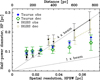 |
Fig. 1. Dependence of the measured HP diameter, HPobs, on spatial resolution (lower x axis) or, equivalently, distance (upper x axis) for the Taurus B211/3 filament at various resolutions as given in Table A.1 (filled blue diamonds with error bars: simple hd estimates; open green diamonds: deconvolved |

Figure 1 also compares the results of the Taurus convergence experiment with the median apparent filament widths derived from Herschel data in the eight nearby clouds of the Arzoumanian et al. (2019) sample (black dots). Overall, the latter measurements are roughly consistent with the linear dependence HPobs ≈ 4 × HPBW (cf. Panopoulou et al. 2022), although the nearest HGBS clouds at d ≲ 200 pc depart from this relation. In particular, it is clear from Fig. 1 that the trend between HPobs and HPBW for the Taurus filament (blue diamonds) is not consistent with a linear dependence with zero intercept. In fact, extrapolating the width measurements to infinite resolution (i.e., HPBW = 0) suggests that the intrinsic HP diameter of the Taurus filament is HPint ≈ 0.08–0.1 pc. Moreover, within the error bars, the Taurus B211/B213 filament provides a fairly good template of the behavior observed in the whole HGBS sample, especially when deconvolved  width estimates are compared.
3. Convergence curves for model filaments
To further clarify the influence of spatial resolution on real data, it is instructive to examine the effect for three simple types of cylindrical model filaments.
The simplest model is a filament with a Gaussian radial profile. In this case, the resolution effect due to convolution with the telescope beam (itself approximated by a Gaussian) is well known. The observed profile is also Gaussian, with a full width at half maximum  , where FWHMint = HPint is the intrinsic HP diameter of the filament profile and HPBW the half-power beam width. Provided that the data have sufficiently high signal to noise, the observations can easily be deconvolved from the telescope beam:
  (a formula referred to as naive deconvolution in the following). It is obvious from this simple example that, in the absence of any deconvolution, one expects a positive correlation between the measured HP widths, FWHMobs, and the spatial resolution of the data, HPBW.
Another simple model is a filament with a power-law radial column density profile, NPL(r)=N0 (r/r0)−m, where m = p − 1 and p = m + 1 (with m > 0) are the exponents of the power law for the column density and density profiles, respectively. In this case, the measured size FWHMobs (or HPobs) of the filament profile is expected to directly scale with, and to be always slightly larger than, the beam size (see, e.g., Adams 1991 and Ladd et al. 1991 for spherical sources). To quantify the FWHMobs versus HPBW correlation, we performed the convolution with a Gaussian beam numerically for a wide range of power-law exponents from p ≳ 1 to p = 3. The results are displayed in Fig. B.1b, which plots the ratio FWHMobs/HPBW ≡ AG(p) as a function of the index, p, of the power-law profile. Observationally, both near-infrared extinction and submillimeter emission studies indicate that the column density profiles of dense molecular filaments have logarithmic slopes in the range 1.5 < p < 2.5 at large radii (e.g., Alves et al. 1998; Lada et al. 1999; Arzoumanian et al. 2011, 2019; Juvela et al. 2012; Stutz & Gould 2016). For this range of p exponents, Fig. B.1b shows that one expects the measured FWHMobs size to be between ∼5% (for p = 2.5) and ∼90% (for p = 1.5) larger than the beam size if the filament profile is a pure power law.
The third model we considered corresponds to a cylindrical filament with a Plummer-like radial column density profile as defined by Eq. (1), which provides a much better fit to the profiles of star-forming filaments such as Taurus B211/B213 (e.g., Palmeirim et al. 2013). We convolved this intrinsic model profile numerically for a wide range of Gaussian beam sizes (expressed in units of the intrinsic HP diameter,  ) and several values of the power-law exponent, p. We then fitted the model function of Eq. (1) to the convolved profiles. The results are illustrated in Fig. 2b, which plots the derived HP widths,
  , as a function of the HP beam resolution HPBW for three relevant values of p (p = 1.5 in blue, p = 2 in red, and p = 2.5 in purple). Here,
  corresponds either to a “direct” hd estimate or to a DHP estimate resulting from the Plummer-like fit in the terminology of Sect. 2 and Table A.1 (these two estimates are essentially indistinguishable). With some care (cf. Sect. 3.3.3 of Arzoumanian et al. 2019), reliable Gaussian fit estimates of the HP width of a Plummer-like profile can also be achieved. This is illustrated in Fig. 2b, which shows that Gaussian fit estimates are only slightly lower (< 10%) than DHP estimates in the p = 1.5 case (for p = 2 and p = 2.5, the Gaussian results are even closer to the DHP estimates).
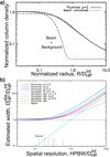 |
Fig. 2. Beam convolution effect for model filaments with Plummer-like radial profiles (see Eq. (1)). (a) Intrinsic Plummer profile with p = 2 on top of a uniform background (solid curve), compared to a Gaussian beam on top of the same background (dash-dotted curve, here assuming |


The dependence of  on HPBW for Plummer models is qualitatively similar to the relation between FWHMobs and HPBW for Gaussian models at small beam sizes (
 ) and asymptotically approaches the linear relation
  expected for filaments with power-law density profiles of index p at large beam sizes (
 ). In the presence of negligible noise, it is possible to derive reliable deconvolved estimates of the HP diameter, denoted
  , by fitting a model corresponding to Eq. (1) convolved with a Gaussian beam to the data. This is illustrated in Fig. 2b, which shows that the Plummer deconvolution process is perfect in the absence of noise. In contrast, naively deconvolved Gaussian FWHMdec values (see above) largely overestimate the intrinsic
  diameters of Plummer models when
  , even in the absence of noise (see the dashed blue, red, and purple curves in Fig. 2b). In the presence of a realistic level of background noise fluctuations (see Appendix C), the Plummer deconvolution process also quickly degrades when
  (see Fig. 3) and
  typically starts to increase with resolution (see the red curve and error bars in Fig. 3b). Plummer estimates
  of the HP width nevertheless remain more accurate than naively deconvolved FWHMdec or hddec values. Moreover, the curves of Fig. 2b can be inverted to provide average deconvolution factors as a function of the observable
  for Plummer profiles with any given p index. This was used to derive the deconvolved estimates shown as light brown symbols in Fig. 1. Comparison between Figs. 1 and 3b supports the conclusion that the Taurus B211/B213 filament has an intrinsic mean HP diameter,
  , corresponding to ∼8 times the HPBW resolution of the Herschel column density map (see Sect. 2 and Palmeirim et al. 2013).
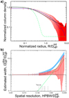 |
Fig. 3. Similar to Fig. 2 but after adding realistic noise to a Plummer-like model filament with p = 1.7. (a) Intrinsic radial profile (solid black curve) compared to the profile that would be observed after convolution with the beam (purple curve with red error bars) in the presence of typical background noise with a Kolmogorov-like power spectrum (see Appendix C). The dash-dotted green curve is the Gaussian beam, here assumed to be |


4. Global comparison with Herschel filaments
We can now confront the simple models of Sect. 3 with the global results obtained on Herschel filaments. Figure 4 shows the mean HP diameters found by Arzoumanian et al. (2019) in eight nearby HGBS clouds and by Schisano et al. (2014) for a sample of filaments from the Herschel Infrared GALactic plane survey (Hi-GAL) as a function of the HPBW spatial resolution of the data in each case. To generate this plot, the Schisano et al. sample was divided into seven bins of spatial resolution between ∼0.1 pc and ∼1 pc (according to filament distance), and the mean filament width in each bin calculated from the results of Schisano et al. (2014). First, it can be seen in Fig. 4 (see also Fig. D.1) that the whole set of Herschel width measurements is not consistent with a single linear relation, such as  , expected for scale-free filaments. In particular, the Herschel data are inconsistent with the linear relation
  advocated by Panopoulou et al. (2022) for the HGBS filaments. The Hi-GAL filaments analyzed by Schisano et al. (2014) have measured HP diameters that are typically 1.9 ± 0.2 times the HPBW spatial resolution (see the green lines in Fig. 4). This is consistent with either pure power-law or unresolved Plummer-like density profiles with logarithmic slopes p ∼ 1.5 at large radii. In contrast, the measured HP widths of nearby HGBS filaments are a factor of ∼4–∼8 times the spatial resolution depending on filament distance, which is incompatible with pure power-law density profiles given the observed range of logarithmic slopes (1.5 < p < 2.5). A much lower FWHMobs/HPBW ratio of ≤1.9 would indeed be expected in the latter case (see Sect. 3 and Fig. B.1b). Quite remarkably, a single Plummer-like model with
  –0.1 pc and p ≈ 1.7 (see the pink curves in Fig. 4) can account for all of the Herschel measurements reasonably well. This suggests that Herschel filaments do have a typical HP width of ∼0.08–0.1 pc and typical power-law wings with p ∼ 1.5–2, but that the flat inner portion of their column density profiles is unresolved by Herschel at the distances of the Hi-GAL filaments in Fig. 4, d ∼ 1–3 kpc.
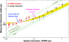 |
Fig. 4. Mean apparent HP width vs. spatial resolution for both HGBS filaments (red squares from Arzoumanian et al. 2019) and Hi-GAL filaments (black circles; Schisano et al. 2014). The vertical error bars correspond to ± the standard deviations of measured widths in each HGBS cloud or Hi-GAL resolution bin. The horizontal error bars represent the Hi-GAL bin widths, which exceed the resolution uncertainties arising from the typical distance uncertainties. The blue curve shows the results of the convergence test performed on the Taurus filament in Sect. 2 (see the blue diamonds in Fig. 1). The pink curves show the theoretical expectations for Plummer-like filaments with a logarithmic density slope p = 1.7 (consistent with the slope of the Taurus filament) and intrinsic HP widths of 0.1 pc and 0.08 pc, respectively (see Sect. 3 and Fig. 2). In the 0.1 pc case, the variations in expected HP width induced by variations in the p index between 1.5 and 2.5 are displayed with yellow shading. Green lines mark 1 × beam, 1.3 × beam, 1.9 × beam, and 4 × beam. |
5. Concluding remarks
The convergence tests we performed on synthetic filaments indicate that filament width measurements are difficult to deconvolve from the telescope beam. In particular, naive Gaussian deconvolution of width measurements obtained on filaments with Plummer-like density profiles is ineffective (cf. Fig. 2b), and proper deconvolution assuming a Plummer model quickly becomes inaccurate in the presence of noise (Fig. 3b). Given the logarithmic slopes 1.5 < p < 2.5 of observed density profiles at large radii, our tests suggest that, without deconvolution, filament width measurements are reasonably accurate and overestimate the intrinsic HP widths of filaments by less than 10%, 15%, and 30% on average when the apparent angular widths exceed the beam HPBW by a factor of ∼8, ∼6, and ∼4, respectively (cf. Fig. 2b). When the apparent filament width is only a factor of ∼2.5 higher than the HPBW, it may overestimate the intrinsic HP width by up to a factor of ∼2–3, and higher-resolution observations are desirable to improve the width estimates. When the apparent filament width is less than a factor of ∼2 broader than the HPBW, the measurements are dominated by the power-law wing of the filament profile and provide little information on the physical width of any flat inner region in the profile.
Overall, our analysis of the effects of finite spatial resolution on filament width measurements reinforces the conclusion of Arzoumanian et al. (2011, 2019) about the existence of a typical HP filament diameter of ∼0.1 pc, at least in the case of nearby, high-contrast filamentary structures (i.e., with a contrast over the local background exceeding ∼50%). Our findings further emphasize the need for a robust theoretical explanation for this common filament width in nearby molecular clouds. While none of the current explanations is fully satisfactory from a theoretical point of view (e.g., Hennebelle & Inutsuka 2019), a promising interpretation is that the common filament width may be linked, at least initially, to the magneto-sonic scale below which interstellar turbulent flows become subsonic and incompressible (primarily solenoidal) in diffuse molecular gas (Federrath 2016; Federrath et al. 2021). The ubiquity of filamentary structures in both diffuse, non-self-gravitating molecular clouds such as the Polaris cirrus (e.g., Miville-Deschênes et al. 2010; André et al. 2010) and numerical simulations of supersonic turbulence without gravity (e.g., Padoan et al. 2001; Pudritz & Kevlahan 2013) suggests that dense molecular filaments somehow result from large-scale turbulent compression of interstellar material before gravity becomes important. Recently, Priestley & Whitworth (2022a),b) argued that the observed distribution of filament widths can be explained if filaments are formed dynamically via converging, mildly supersonic flows arising from large-scale turbulent motions. As pointed out by Jaupart & Chabrier (2021), the sonic scale is directly related to the correlation length, lc, of initial density fluctuations generated by supersonic isothermal turbulence (before gravity starts to play a significant role). In other words, the typical filament width found in Herschel observations may correspond to the average size of the most correlated structures produced by turbulence in diffuse molecular clouds. We stress that there is no contradiction between the existence of a finite correlation length for the (column) density field and the essentially scale-free power spectrum observed for column density fluctuations (e.g., Miville-Deschênes et al. 2010), since the correlation length, lc ∝ P(0)/∫P(k) dk, only depends on the integral of the power spectrum, ∫P(k) dk (i.e., the variance of the density field) and its value at zero spatial frequency, P(0), but not on the detailed shape of the power spectrum, P(k). Using column density data from the HGBS, Jaupart & Chabrier (2022) made rough estimates of the turbulent correlation length in the Polaris and Orion B clouds. They find values broadly consistent with lc ∼ 0.1 pc, albeit with large uncertainties (up to a factor of ∼3–10). Following the method introduced by Houde et al. (2009), independent estimates of the magnetized turbulent correlation length have also been obtained from analyses of the angular dispersion function of polarization angles in recent high-quality dust polarimetry maps. For instance, using SOFIA HAWC+ data, Guerra et al. (2021) find lc ∼ 0.05–0.15 pc in most of the Orion OMC-1 field they observed, and Li et al. (2022) estimate lc ∼ 0.075–0.095 pc in a significant portion of the Taurus B211 filament. One merit of interpreting the typical filament width as the turbulent correlation length is that it naturally accounts for the dispersion of width measurements around the mean ∼0.1 pc value (both along the crest of each filament and from filament to filament), since the initial filament widths are only expected to match the sonic scale in a statistical sense. This interpretation is incomplete, however, because it does not explain how self-gravitating, thermally supercritical filaments maintain a roughly constant inner width while evolving. Further work is therefore clearly needed to provide a more complete explanation and clarify the role of the turbulent correlation length.
Acknowledgments
We thank E. Schisano for kindly providing the width measurements from Schisano et al. (2014), used in Figs. 4 and D.1 of this paper. We acknowledge support from the French national programs of CNRS/INSU on stellar and ISM physics (PNPS and PCMI). PP acknowledges support from FCT/MCTES through Portuguese national funds (PIDDAC) by grant UID/FIS/04434/2019 and from fellowship SFRH/BPD/110176/2015 funded by FCT (Portugal) and POPH/FSE (EC). This study has made use of data from the Herschel Gould Belt Survey (HGBS), a Herschel Key Program carried out by SPIRE Specialist Astronomy Group 3 (SAG 3), scientists of institutes in the PACS Consortium (CEA Saclay, INAF-IFSI Rome and INAF-Arcetri, KU Leuven, MPIA Heidelberg), and scientists of the Herschel Science Centre (HSC).
References
- Adams, F. C. 1991, ApJ, 382, 544 [Google Scholar]
- Alves, J., Lada, C. J., Lada, E. A., Kenyon, S. J., & Phelps, R. 1998, ApJ, 506, 292 [NASA ADS] [CrossRef] [Google Scholar]
- André, P., Men’shchikov, A., Bontemps, S., et al. 2010, A&A, 518, L102 [NASA ADS] [CrossRef] [EDP Sciences] [Google Scholar]
- André, P., Di Francesco, J., Ward-Thompson, D., et al. 2014, in Protostars and Planets VI, eds. H. Beuther, R. Klessen, C. Dullemond, et al., 27 [Google Scholar]
- André, P., Arzoumanian, D., Könyves, V., et al. 2019, A&A, 629, L4 [NASA ADS] [CrossRef] [EDP Sciences] [Google Scholar]
- Aniano, G., Draine, B. T., Gordon, K. D., & Sandstrom, K. 2011, PASP, 123, 1218 [Google Scholar]
- Arzoumanian, D., André, P., Didelon, P., et al. 2011, A&A, 529, L6 [NASA ADS] [CrossRef] [EDP Sciences] [Google Scholar]
- Arzoumanian, D., André, P., Könyves, V., et al. 2019, A&A, 621, A42 [NASA ADS] [CrossRef] [EDP Sciences] [Google Scholar]
- Di Francesco, J., Keown, J., Fallscheer, C., et al. 2020, ApJ, 904, 172 [NASA ADS] [CrossRef] [Google Scholar]
- Federrath, C. 2016, MNRAS, 457, 375 [Google Scholar]
- Federrath, C., Klessen, R. S., Iapichino, L., & Beattie, J. R. 2021, Nat. Astron., 5, 365 [NASA ADS] [CrossRef] [Google Scholar]
- Guerra, J. A., Chuss, D. T., Dowell, C. D., et al. 2021, ApJ, 908, 98 [NASA ADS] [CrossRef] [Google Scholar]
- Hacar, A., Clark, S., Heitsch, F., et al. 2022, in Protostars and Planets VII, eds. S. Inutsuka, Y. Aikawa, T. Muto, et al., in press [arXiv:2203.09562] [Google Scholar]
- Hennebelle, P., & Inutsuka, S.-I. 2019, Front Astron. Space Sci., 6, 5 [CrossRef] [Google Scholar]
- Hill, T., Motte, F., Didelon, P., et al. 2011, A&A, 533, A94 [NASA ADS] [CrossRef] [EDP Sciences] [Google Scholar]
- Houde, M., Vaillancourt, J. E., Hildebrand, R. H., Chitsazzadeh, S., & Kirby, L. 2009, ApJ, 706, 1504 [Google Scholar]
- Inutsuka, S.-I., & Miyama, S. M. 1992, ApJ, 388, 392 [CrossRef] [Google Scholar]
- Jaupart, E., & Chabrier, G. 2021, ApJ, 922, L36 [NASA ADS] [CrossRef] [Google Scholar]
- Jaupart, E., & Chabrier, G. 2022, A&A, 663, A113 [NASA ADS] [CrossRef] [EDP Sciences] [Google Scholar]
- Juvela, M., Ristorcelli, I., Pagani, L., et al. 2012, A&A, 541, A12 [NASA ADS] [CrossRef] [EDP Sciences] [Google Scholar]
- Könyves, V., André, P., Men’shchikov, A., et al. 2015, A&A, 584, A91 [Google Scholar]
- Lada, C. J., Alves, J., & Lada, E. A. 1999, ApJ, 512, 250 [NASA ADS] [CrossRef] [Google Scholar]
- Ladd, E. F., Adams, F. C., Casey, S., et al. 1991, ApJ, 382, 555 [NASA ADS] [CrossRef] [Google Scholar]
- Li, P. S., Lopez-Rodriguez, E., Ajeddig, H., et al. 2022, MNRAS, 510, 6085 [CrossRef] [Google Scholar]
- Marsh, K. A., Kirk, J. M., André, P., et al. 2016, MNRAS, 459, 342 [Google Scholar]
- Miville-Deschênes, M.-A., Martin, P. G., Abergel, A., et al. 2010, A&A, 518, L104 [CrossRef] [EDP Sciences] [Google Scholar]
- Molinari, S., Swinyard, B., Bally, J., et al. 2010, A&A, 518, L100 [NASA ADS] [CrossRef] [EDP Sciences] [Google Scholar]
- Nagasawa, M. 1987, Progr. Theoret. Phys., 77, 635 [NASA ADS] [CrossRef] [Google Scholar]
- Ostriker, J. 1964, ApJ, 140, 1056 [Google Scholar]
- Padoan, P., Juvela, M., Goodman, A. A., & Nordlund, Å. 2001, ApJ, 553, 227 [NASA ADS] [CrossRef] [Google Scholar]
- Palmeirim, P., André, P., Kirk, J., et al. 2013, A&A, 550, A38 [NASA ADS] [CrossRef] [EDP Sciences] [Google Scholar]
- Panopoulou, G. V., Clark, S. E., Hacar, A., et al. 2022, A&A, 657, L13 [NASA ADS] [CrossRef] [EDP Sciences] [Google Scholar]
- Pineda, J. E., Arzoumanian, D., André, P., et al. 2022, in Protostars and Planets VII, eds. S. Inutsuka, Y. Aikawa, T. Muto, et al., in press [arXiv:2205.03935] [Google Scholar]
- Priestley, F. D., & Whitworth, A. P. 2022a, MNRAS, 509, 1494 [Google Scholar]
- Priestley, F. D., & Whitworth, A. P. 2022b, MNRAS, 512, 1407 [NASA ADS] [CrossRef] [Google Scholar]
- Pudritz, R. E., & Kevlahan, N. K.-R. 2013, Phil. Trans. R. Soc. A, 371, 20248 [Google Scholar]
- Raskutti, S., Ostriker, E. C., & Skinner, M. A. 2016, ApJ, 829, 130 [NASA ADS] [CrossRef] [Google Scholar]
- Schisano, E., Rygl, K. L. J., Molinari, S., et al. 2014, ApJ, 791, 27 [Google Scholar]
- Stutz, A. M., & Gould, A. 2016, A&A, 590, A2 [NASA ADS] [CrossRef] [EDP Sciences] [Google Scholar]
Appendix A: Results of the convergence test on the Taurus filament
Here, we provide a table with the detailed results of the convergence test described in Sect. 2 on the Taurus B211/B213 filament.
Estimated widths of the B211/B213 filament at various resolutions.
Appendix B: Tests on model filaments with power-law profiles
Figure B.1 illustrates and summarizes the results of the simple tests we performed for model filaments with power-law column density profiles (see Sect. 3).
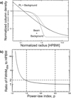 |
Fig. B.1. Beam convolution effect for model filaments with power-law (PL) radial profiles. (a) Example of an intrinsic PL radial profile on top of a uniform background (solid curve), compared to a Gaussian beam on top of the same background (dash-dotted curve), and to the model PL profile after convolution with the beam (dashed curve). The thin solid line marks the HP level of both the convolved PL profile and the beam. (b) Plot of the ratio FWHMobs/HPBW ≡ AG(p) against the logarithmic slope of the radial density profile, p, for PL filaments. The two vertical dashed lines bracket the range of PL indices for observed filaments at large radii (1.5 < p < 2.5). |
Appendix C: Generating synthetic data for Plummer-like filaments with realistic background noise
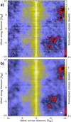 |
Fig. C.1. Two examples of synthetic column density maps of a Plummer model filament with p = 1.7 embedded in a structured background with a cirrus-like P(k)∝k−2.7 power spectrum (see text). (a) Model image “observed” at a HPBW resolution corresponding to |


Here, we provide details on the method employed in Sect. 3 to construct synthetic data corresponding to the observation of a cylindrical model filament with a Plummer-like column density profile (cf. Eq. 1) in the presence of realistic background “noise” fluctuations. The noise in Herschel maps of molecular clouds at wavelengths λ ≥ 160 μm is usually dominated by the “structure noise” induced by the fluctuations in the background cloud emission. Moreover, the power spectrum measured for far-infrared images of interstellar clouds is typically Kolmogorov-like with P(k)∝k−2.7 (e.g., Miville-Deschênes et al. 2010). For the tests illustrated in Fig. 3, we thus constructed a series of synthetic column density maps by adding randomly generated maps of background fluctuations with such a P(k)∝k−2.7 power spectrum to the column density map of a Plummer model filament with a logarithmic density slope p = 1.7 (assumed to lie in the plane of the sky). The standard deviation of the background noise map was fixed to one-tenth of the central column density of the model filament. We also introduced realistic random fluctuations of the intrinsic HP diameter of the model filament along its length; these random fluctuations had a lognormal distribution centered at  with a standard deviation of 0.3 dex, as observed for HGBS filaments (see Fig. 7 of Pineda et al. 2022). The synthetic maps were smoothed to a wide range of effective resolutions by convolving them with circular Gaussian kernels. Two examples of such smoothed column density maps are displayed in Fig. C.1, including the map corresponding to the filament column density profile shown in Fig. 3a observed at a resolution
  . For each synthetic column density map and each resolution, the distribution of resulting radial profiles along the model filament was derived, which allowed us to construct a mean radial profile such as the one of Fig. 3a, with error bars corresponding to the standard deviation of radial profiles at each radius. The model represented by Eq. (1), both before and after convolution with a Gaussian beam, was then fitted to each of these mean radial profiles to provide
  and
and  estimates of the filament HP width at each resolution. A total of 1000 realizations of the random background fluctuations were generated to construct the plot shown in Fig. 3b, which shows the mean
  and
and  values averaged over the 1000 realizations as a function of HPBW resolution. The error bars correspond to the standard deviations measured for the distributions of values at each resolution.
Appendix D: Distribution of Herschel filament widths
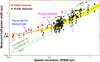 |
Fig. D.1. Mean apparent HP width (without any deconvolution) versus spatial resolution for both HGBS filaments (red squares from Arzoumanian et al. 2019) and Hi-GAL filaments (black circles from Schisano et al. 2014). The red error bars correspond to ± the standard deviations of measured widths in each HGBS cloud. The black error bars correspond to ± the standard deviation of individual width estimates along each Hi-GAL filament in the Schisano et al. sample. The lines, curves, and yellow shading are the same as in Fig. 4. |
In this appendix, we show a plot of apparent HP width against spatial resolution similar to Fig. 4, but where we display all individual width measurements from Schisano et al. (2014) instead of binning the distribution of Hi-GAL widths (Fig. D.1). In this way, the full scatter of Hi-GAL width measurements can be better appreciated. As in Figs. 1 and 4, the distances adopted in Fig. D.1 for the HGBS clouds are those indicated by Gaia data (cf. Panopoulou et al. 2022). The HGBS cloud with the most uncertain distance (IC5146) is represented by two connected red symbols. The distances adopted for the Hi-GAL filaments are those used by Schisano et al. (2014), whose typical uncertainties are smaller than the horizontal error bars in Fig. 4.
Appendix E: Effect of a non-Gaussian beam
The synthetic data discussed in Sect. 3 were smoothed to various effective resolutions assuming a strictly Gaussian beam. In reality, the Herschel beams are not strictly Gaussian and include low-level non-Gaussian features (e.g., Aniano et al. 2011). To assess the potential impact of these non-Gaussian features on the tests performed in Sect. 3, we repeated the numerical experiment summarized in Fig. 2 assuming that the effective beam of Herschel column density maps had a shape similar to that of the true Herschel/SPIRE beam at 250 μm (see the dash-dotted purple curve in Fig. E.1a). As shown in Fig. E.1b, the curves of derived HP widths (Plummer  and Gaussian FWHMobs) as a function of beam resolution (HPBW) are almost identical to those in Fig. 2b. This indicates that the non-Gaussian structure of the Herschel beams has very little influence on the results presented in Sect. 3. The only visible effect is that the Plummer deconvolution process and resulting
  estimates of the filament width (see dashed black lines in Fig. E.1b) are no longer perfectly accurate, even in the absence of noise. This is hardly surprising since accurate beam deconvolution requires both high signal to noise and excellent knowledge of the beam shape.
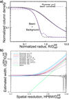 |
Fig. E.1. Similar to Fig. 2 but assuming that the effective beam corresponds to the real SPIRE 250 μm beam as opposed to a strictly Gaussian beam. (a) Convolution of a model filament with a p = 2 Plummer-like radial profile by a non-Gaussian beam corresponding to the SPIRE beam at 250 μm. The dash-dotted purple curve shows this non-Gaussian beam on top of the same uniform background as in Fig. 2a. The dashed purple curve is the filament profile after convolution with this beam (assuming the same |

All Tables
All Figures
|
Fig. 1. Dependence of the measured HP diameter, HPobs, on spatial resolution (lower x axis) or, equivalently, distance (upper x axis) for the Taurus B211/3 filament at various resolutions as given in Table A.1 (filled blue diamonds with error bars: simple hd estimates; open green diamonds: deconvolved |
| In the text | |
|
Fig. 2. Beam convolution effect for model filaments with Plummer-like radial profiles (see Eq. (1)). (a) Intrinsic Plummer profile with p = 2 on top of a uniform background (solid curve), compared to a Gaussian beam on top of the same background (dash-dotted curve, here assuming |
| In the text | |
|
Fig. 3. Similar to Fig. 2 but after adding realistic noise to a Plummer-like model filament with p = 1.7. (a) Intrinsic radial profile (solid black curve) compared to the profile that would be observed after convolution with the beam (purple curve with red error bars) in the presence of typical background noise with a Kolmogorov-like power spectrum (see Appendix C). The dash-dotted green curve is the Gaussian beam, here assumed to be |
| In the text | |
|
Fig. 4. Mean apparent HP width vs. spatial resolution for both HGBS filaments (red squares from Arzoumanian et al. 2019) and Hi-GAL filaments (black circles; Schisano et al. 2014). The vertical error bars correspond to ± the standard deviations of measured widths in each HGBS cloud or Hi-GAL resolution bin. The horizontal error bars represent the Hi-GAL bin widths, which exceed the resolution uncertainties arising from the typical distance uncertainties. The blue curve shows the results of the convergence test performed on the Taurus filament in Sect. 2 (see the blue diamonds in Fig. 1). The pink curves show the theoretical expectations for Plummer-like filaments with a logarithmic density slope p = 1.7 (consistent with the slope of the Taurus filament) and intrinsic HP widths of 0.1 pc and 0.08 pc, respectively (see Sect. 3 and Fig. 2). In the 0.1 pc case, the variations in expected HP width induced by variations in the p index between 1.5 and 2.5 are displayed with yellow shading. Green lines mark 1 × beam, 1.3 × beam, 1.9 × beam, and 4 × beam. |
| In the text | |
|
Fig. B.1. Beam convolution effect for model filaments with power-law (PL) radial profiles. (a) Example of an intrinsic PL radial profile on top of a uniform background (solid curve), compared to a Gaussian beam on top of the same background (dash-dotted curve), and to the model PL profile after convolution with the beam (dashed curve). The thin solid line marks the HP level of both the convolved PL profile and the beam. (b) Plot of the ratio FWHMobs/HPBW ≡ AG(p) against the logarithmic slope of the radial density profile, p, for PL filaments. The two vertical dashed lines bracket the range of PL indices for observed filaments at large radii (1.5 < p < 2.5). |
| In the text | |
|
Fig. C.1. Two examples of synthetic column density maps of a Plummer model filament with p = 1.7 embedded in a structured background with a cirrus-like P(k)∝k−2.7 power spectrum (see text). (a) Model image “observed” at a HPBW resolution corresponding to |
| In the text | |
|
Fig. D.1. Mean apparent HP width (without any deconvolution) versus spatial resolution for both HGBS filaments (red squares from Arzoumanian et al. 2019) and Hi-GAL filaments (black circles from Schisano et al. 2014). The red error bars correspond to ± the standard deviations of measured widths in each HGBS cloud. The black error bars correspond to ± the standard deviation of individual width estimates along each Hi-GAL filament in the Schisano et al. sample. The lines, curves, and yellow shading are the same as in Fig. 4. |
| In the text | |
|
Fig. E.1. Similar to Fig. 2 but assuming that the effective beam corresponds to the real SPIRE 250 μm beam as opposed to a strictly Gaussian beam. (a) Convolution of a model filament with a p = 2 Plummer-like radial profile by a non-Gaussian beam corresponding to the SPIRE beam at 250 μm. The dash-dotted purple curve shows this non-Gaussian beam on top of the same uniform background as in Fig. 2a. The dashed purple curve is the filament profile after convolution with this beam (assuming the same |
| In the text | |
Current usage metrics show cumulative count of Article Views (full-text article views including HTML views, PDF and ePub downloads, according to the available data) and Abstracts Views on Vision4Press platform.
Data correspond to usage on the plateform after 2015. The current usage metrics is available 48-96 hours after online publication and is updated daily on week days.
Initial download of the metrics may take a while.