| Issue |
A&A
Volume 649, May 2021
|
|
|---|---|---|
| Article Number | A84 | |
| Number of page(s) | 15 | |
| Section | Interstellar and circumstellar matter | |
| DOI | https://doi.org/10.1051/0004-6361/201936388 | |
| Published online | 18 May 2021 | |
Spatial distribution of the aromatic and aliphatic carbonaceous nanograin features in the protoplanetary disk around HD 100546★
1
Université Paris-Saclay, CNRS, Institut d’Astrophysique Spatiale,
91405
Orsay, France
e-mail: emilie.habart@ias.u-psud.fr
2
IRFU/SAp Service D’Astrophysique, CEA,
Gif-sur-Yvette, France
3
Canadian Institute for Theoretical Astrophysics, University of Toronto,
60 St. George Street,
Toronto,
ON
M5S 3H8, Canada
Received:
26
July
2019
Accepted:
25
August
2020
Context. Carbonaceous nanograins are present at the surface of protoplanetary disks around Herbig Ae/Be stars, where most of the ultraviolet energy from the central star is dissipated. Efficiently coupled to the gas, they are unavoidable to understand the physics and chemistry of these disks. Furthermore, nanograins are able to trace the outer flaring parts of the disk and possibly the gaps from which the larger grains are missing. However, their evolution through the disks, from internal to external regions, is only poorly understood so far.
Aims. Our aim is to examine the spatial distribution and evolution of the nanodust emission in the emblematic (pre-)transitional protoplanetary disk HD 100546. This disk shows many structures (annular gaps, rings, and spirals) and reveals very rich carbon nanodust spectroscopic signatures (aromatic, aliphatic) in a wide spatial range of the disk (~20−200 au).
Methods. We analysed adaptive optics spectroscopic observations in the 3–4 μm range (angular resolution of ~0.1′′) and imaging and spectroscopic observations in the 8–12 μm range (angular resolution of ~0.3′′). The hyperspectral cube was decomposed into a sum of spatially coherent dust components using a Gaussian decomposition algorithm. We compared the data to model predictions using the heterogeneous dust evolution model for interstellar solids (THEMIS), which is integrated in the radiative transfer code POLARIS by calculating the thermal and stochastic heating of micro- and nanometre-sized dust grains for a given disk structure.
Results. We find that the aromatic features at 3.3, 8.6, and 11.3 μm, and the aliphatic features between 3.4 and 3.5 μm are spatially extended; each band shows a specific morphology dependent on the local physical conditions. The aliphatic-to-aromatic band ratio, 3.4/3.3, increases with the distance from the star from ~0.2 (at 0.2′′ or 20 au) to ~0.45 (at 1′′ or 100 au), suggesting UV processing. In the 8–12 μm observed spectra, several features characteristic of aromatic particles and crystalline silicates are detected. Their relative contribution changes with the distance to the star. The model predicts that the features and adjacent continuum are due to different combinations of grain sub-populations, in most cases with a high dependence on the intensity of the UV field. The model reproduces the spatial emission profiles of the bands well, except for the inner 20-40 au, where the observed emission of the 3.3 and 3.4 μm bands is, unlike the predictions, flat and no longer increases with the UV field.
Conclusions. With our approach that combines observational data in the near- to mid-IR and disk modelling, we deliver constraints on the spatial distribution of nano-dust particles as a function of the disk structure and radiation field.
Key words: protoplanetary disks / infrared: planetary systems
The reduced NACO data spectral cube and VISIR long-slit spectrum are only available at the CDS via anonymous ftp to cdsarc.u-strasbg.fr (130.79.128.5) or via http://cdsarc.u-strasbg.fr/viz-bin/cat/J/A+A/649/A84
© E. Habart et al. 2021
 Open Access article, published by EDP Sciences, under the terms of the Creative Commons Attribution License (https://creativecommons.org/licenses/by/4.0), which permits unrestricted use, distribution, and reproduction in any medium, provided the original work is properly cited.
1 Introduction
The objective of this article is to study the spatial distribution and possible changes in the properties of carbon nano-dust in protoplanetary disks (PPDs). Carbon nanodust, detected under more or less organised structures and different ionisation states, constitutes a major component of dust in the interstellar and circumstellar environments. Vibrational emission bands in the near- to mid-IR from nanocarbon dust have been observed towards PPDs around most of the Herbig Ae stars, about half of the Herbig Be stars, and a few T-Tauri stars (e.g. Brooke et al. 1993; Acke & van den Ancker 2004; Acke et al. 2010; Seok & Li 2017). In contrast to large grains, these tiny and numerous carbon grains are well coupled to the gas and do not settle towards disk midplanes. This results in different spatial distributions in which tiny grains are present at the disk surfaces (e.g. Meeus et al. 2001; Habart et al. 2004; Lagage et al. 2006) and in the cavity or gaps from which the pebbles are missing (e.g. Geers et al. 2007; Kraus et al. 2013; Klarmann et al. 2017; Kluska et al. 2018; Maaskant et al. 2013). The very small carbon grains in the irradiated disk layers may have strong consequences (e.g. Gorti & Hollenbach 2008). As in the irradiated regions of the interstellar medium, they are the prevalent contributors to the energetic balance because they are very efficient at absorbing UV photons and heating the gas through the photoelectric effect. The highest fluxes of lines tracing the warm gas (e.g. [OI] 63 and [OI] 145 μm, H2 0-0 S(1), and high-J CO) are found in PPDs that show a large amount of flaring and high aromatic band strength (e.g. Meeus et al. 2013). Moreover, due to their large effective surface area, they may dominate the catalytic formation of key molecules as H2 and the charge balance. The disk structure may further depend on the level of nanograins that are coupled with the gas. Characterising the size and properties of these tiny grains through the disks, from internal to external regions, is thus of prime importance to understand the structure and evolution of PPDs.
Boutéraon et al. (2019) recently reported several spatially extended near-IR spectral features that are related to aromatic and aliphatic hydrocarbon material in PPDs around Herbig stars, from 10 to 50–100 au, and even in inner gaps that are devoid of large grains. The correlation between aliphatic and aromatic CH stretching bands suggested common carriers for all features. Because these hydrocarbon nano-particles are a priori easily destroyed by UV photons (e.g. Muñoz Caro et al. 2001; Mennella et al. 2001; Gadallah et al. 2012), this probably implies that they are continuously replenished at the disk surfaces. In continuity of the Boutéraon et al. (2019) study, we investigate here the nanodust properties in disks with a decomposition tool applied to spectra, complementary observations at longer mid-IR wavelengths, and the coupling of THEMIS (The Heterogeneous dust Evolution Model for Interstellar Solids, Jones et al. 2017) with the radiative transfer code POLARIS (POLArized RadIation Simulator, Reissl et al. 2016; Brauer et al. 2017). We focus on the emblematic protoplanetary disk HD 100546, which is in transitional phase from a gas-rich to a dust debris disk (e.g. Bouwman et al. 2003).
The paper is organised as follows. Section 2 provides a description of the protoplanetary disk HD 100546. In Sect. 3 we analyse the adaptive optics spectroscopic observations in the L band obtained with NAOS-CONICA (NaCo) at the VLT (Very Large Telescope) using the Regularized Optimization for HyperSpectral Analysis (ROHSA) tool for the decomposition. Imaging and spectroscopic observations obtained with VISIR (VLT Imager and Spectrometer for mid Infrared) at the VLT are also presented and analysed. In Sect. 4 the disk modelling with the THEMIS dust model and the radiative transfer code POLARIS are presented. In Sect. 5 we compare the model predictions to the NaCo and VISIR observations. In Sect. 6 our results for the nanodust evolution are discussed.
2 HD 100546
HD 100546 is one of the closest very well studied Herbig Be stars (d = 110 ± 4 pc, Gaia Collaboration 2018). It shows clear evidence of a large flared disk, and based on images obtained with the Hubble Space Telescope (HST) and ground-based high-contrast images, an elliptical structure was detected that extends up to 350–380 au (Augereau et al. 2001). Furthermore, multiple-armed spiral patterns were identified as well (Grady et al. 2001; Ardila et al. 2007; Boccaletti et al. 2013; Avenhaus et al. 2014). The disk position angle measurements found in the literature range from ~ 130 to 160° (Grady et al. 2001; Pantin et al. 2000; Ardila et al. 2007; Panić et al. 2014; Augereau et al. 2001; Avenhaus et al. 2014), and the inclination of the disk is smaller than 50° (Avenhaus et al. 2014). An inner dust disk extending from ~0.2 to ~ 1−4 au was resolved using near-IR interferometry (Benisty et al. 2010; Tatulli et al. 2011; Mulders et al. 2013; Panić et al. 2014). The (pre-)transitional nature of HD 100546 was initially proposed by Bouwman et al. (2003) based on a spectral energy distribution (SED) analysis. The presence of a gap extending up to 10–15 au has been confirmed by mid-IR interferometry (Liu et al. 2003; Panić et al. 2014), spectroscopy in the UV and near-IR (Grady et al. 2005; Brittain et al. 2009; van der Plas et al. 2009), and high-resolution polarimetric imaging in the optical and near-IR (Avenhaus et al. 2014; Quanz et al. 2015; Garufi et al. 2016; Follette et al. 2017). Recent ALMA observations reveal an asymmetric ring between ~ 20−40 au with largely optically thin dust emission (Pineda et al. 2019). A central compact emission is also detected, which arises from the inner central disk, which given its mass and the accretion rate onto the star, must be replenished with material from the outer disk (Pineda et al. 2019). Miley et al. (2019) presented the first detection of C18 O in this disk, which spatially coincides with the spiral arms, and derived a lower-limit on the total gas mass (around 1% of the stellar mass) and a gas-to-dust mass ratio in the disk of ~ 20 assuming interstellar medium (ISM) abundances of C18O relative to H2. HD 100546 is also one of the few cases where protoplanet candidates have been suggested (e.g. Quanz et al. 2015; Currie et al. 2015), although this is still being debated (e.g. Follette et al. 2017; Rameau et al. 2017; Pérez et al. 2020). Recently, Pérez et al. (2020) detected a compact 1.3 mm continuum dust emission source that lies in the middle of the HD 100546 cavity (0.051′′ from the central star). This is compatible with circumplanetary disk emission.
On the other hand, this disk with high density and temperature coupled with high UV flux on its surface presents very rich IR spectral features and variations in the chemical and physical dust structural properties. HD 100546 is the first disk in which crystalline silicates and intense aromatic bands between 3 and 13 μm have been detected (Hu et al. 1989; Malfait et al. 1998). The carriers of these bands can be attributed to polyaromatic species and associated with an emission mechanism based on polycyclic aromatic hydrocarbon (PAH) photophysics. These intense bands are blended with many fainter sub-bands (e.g. Acke et al. 2010; Boutéraon et al. 2019) and are spatially extended on a few 100 au scale (van Boekel et al. 2004; Habart et al. 2006). Boutéraon et al. (2019) presented the diversity of the sub-features in the 3–4 μm range where C-H vibrational modes are observed. These modes are particularly interesting because they characterise the bonds between carbon and hydrogen atoms that vary according to their local environment and strongly depend on the hydrocarbon grain sizes. Constraints can thus be derived for the grain size distribution and the hydrogen-to-carbon ratio in the grains, depending on their more or less aromatic or aliphatic nature.
Seok & Li (2017) extracted the global mid-IR nanocarbon dust spectrum of HD 100546 and analysed it using the Li & Draine (2001) and Draine & Li (2007) astro-PAH model. They found that most of the PAHs are neutral, with a low ionisation fraction of 0.2, and a mass distribution that peaks at 5.64 Å (log-normal size distribution centred at 0.5 Å with a width of 0.2), similar to what is required to explain diffuse ISM observations. These results agree with the analysis made by Boutéraon et al. (2019) using the THEMIS amorphous hydrogenated carbon nano-grains. Assuming that all PAHs are located at 10 au from the central star, Seok & Li (2017) found a total PAH mass in the disk of MPAH = 5.37 × 10⁻⁶ M⊕.
Finally, HD 100546 is one of the few Herbig Ae/Be stars to show a strong luminosity in the aromatic bands and warm gas lines such as the rotational and rovibrational lines of H2 (Carmona et al. 2011), CH+ (Thi et al. 2011) and CO (Meeus et al. 2012, 2013) at the same time. This strongly suggests that the carriers of the aromatic bands that efficiently absorb the stellar UV radiation are one if not the main source of the gas heating through photoelectric effect in the warm disk surfaces (e.g. Meeus et al. 2013).
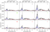 |
Fig. 1 Mosaic of near-IR emission spectra of HD 100546 between 3.2 and 3.8 μm. Their location (coloured symbols) is reported in Fig. 2. The result of the decomposition with ROHSA (black) is overplotted on NaCo data (grey). Gaussians related to the 3.3 μm aromatic feature are shown in blue, and those related to the 3.4 μm aliphatic feature in cyan. Other features are plotted in brown. |
3 NaCo and VISIR observations
In the next sections, we analyse the NaCo spectroscopic observations. We analyze the VISIR imaging and spectroscopic observationsin a second step.
3.1 NaCo observations and data decomposition using ROHSA
3.1.1 Observations
NaCo observations were performed using a long slit in the L band, between 3.20 and 3.76 μm, with the adaptive optics system NaCo at the VLT. The on-sky projection of the slit is 28′′ long and 0.086′′ wide, whichcorresponds to the diffraction limit in this wavelength range. The pixel scale is 0.0547′′ and the spectral resolution is R = λ∕Δλ ~ 1000. We took nine slit positions, one centred on the star and the other slits shifted by a half width. Nine positions allowed us to extract a spectral cube on an area star-centred of 2′′ × 0.354′′. The long slit was aligned with the major axis of the disk as resolved in scattered light (Augereau et al. 2001; Grady et al. 2001) with a position angle of 160° measured north to east. The dataset reference is 075.C-0624(A), and observations characteristics and data reduction are summarised in Boutéraon et al. (2019).
3.1.2 Spectral cube decomposition using ROHSA
The NaCo spectral cube was decomposed using ROHSA in order to produce maps in the various dust features observed in the 3.20 to 3.76 μm spectral range. ROHSA is based on a regularised non-linear criterion that takes the spatial coherence of the emission into account (Marchal et al. 2019). To fit the cube, a multi-resolution process from coarse to fine grid was used. First, a Gaussian decomposition with a fixed number of Gaussians N was performed on a spatially averaged version of the data (corresponding at the first iteration to the mean spectrum of the cube). So far, the method is similar to the one described in Boutéraon et al. (2019). The solution was then interpolated step by step at higher resolution until the initial resolution of the observations was reached. At each step of this process, the algorithm converged towards a solution that for each Gaussian was spatially coherent. Additionally, ROHSA minimises the variance of the dispersion of each component, meaning that on average, a Gaussian has a similar width across the disk. Because the signatures are strongly spectrally blinded, this minimisation is essential to separate them. This commanded spatial coherence allows removing the random noise. The central parts of the spectral cube are not provided to ROHSA because the signal-to-noise ratio in the bands is too low due to a strong continuum emission.
3.1.3 Results
Figure 1 shows the result of the decomposition for spectra from different locations in the disk (Fig. 2). Twenty-eight Gaussians are needed to fully describe the signal and to fit the spectra towards the entire cube. We assumed that a physical signature can be reproduced by several Gaussians. We gathered Gaussians according to their central wavelength as in Boutéraon et al. (2019), who considered six features related to carbonaceous materials: one aromatic signature at 3.3 μm, and five aliphatic ones at 3.4, 3.43, 3.46, 3.52, and 3.56 μm (Fig. A.1). The remaining Gaussians correspond to the hydrogen-recombination and telluric lines. We removed the Gaussians that are expected to be related to telluric bands.
For the 3.3 μm aromatic band, we considered two Gaussians, one narrow Gaussian centred at 3.297 μm, and one broader Gaussian centred at 3.306 μm. As discussedin Boutéraon et al. (2019), these two components could originate from two distinct types of bonding: aromatic and olefinic, respectively. For the 3.4 μm aliphatic band, we considered three Gaussians, two narrow Gaussians centred at 3.398 and 3.409 μm, and one broader Gaussian centred at 3.403 μm. We focus onthese two features because they are brighter and less strongly blended than the others.
Figure 2 shows the maps in the 3.3 μm aromatic and 3.4 μm aliphatic emission bands, and Fig. 3 shows their average spatial emission profiles according to the distance d of each pixel from the star. These two emission bands, due to transient emission after UV photon absorption, may trace the surface of the disk where most of the UV energy is dissipated and converted into near- to mid-IR emission by dust. The carriers are stochastically heated, therefore the band intensities are proportional to the strength of the far-UV radiation field given by G0 expressed in units of the average interstellar radiation field, 1.6 × 10⁻³ erg s−1 cm−2 (Habing 1968). The band emission is thus expected to be much more spatially extended than the IR thermal emission of large grains at thermal equilibrium. The maps and spatial profiles show that the emission in the 3.3 and 3.4 μm bands is in fact spatially extended up to ~1′′ (or ~ 110 au) for both bands. We observe an emission peak between 0.2′′ and 0.4′′, or 22 and 44 au, located just after the inner edge of the outer disk at about 10–15 au. The decrease in emission for d > 0.4′′ roughly follows a 1∕d2 law (dashed lines in Fig. 3), which corresponds to the dilution law of the far-UV radiation field strength, G0.
Correlated intensities of aromatic and aliphatic features argue in favour of a common nature of the carriers: stochastically heated nanoparticles (see also Boutéraon et al. 2019). Beyond 0.4′′, the intensity of the 3.3 μm aromatic band decreases slightly more rapidly than that of the 3.4 μm aliphatic band. This could reflect size or composition changes in the nanoparticles. Closer to the star, between 0.2′′ and 0.4′′, the emission is flat and no longer varies with G0. This can be due to disk structure effects, for instance cavity effects, shadows at the inner edge of the outer disk, or changes in the properties of the nanoparticles, for example abundance and size. At large scales, the structure seen in the nanodust emission appears to match the elliptical structure detected in the stellar light scattered by (sub-)micron grains (e.g. Augereau et al. 2001). This is consistent with the expectation that the nanodust emission traces the disk surface.
The maps in the aromatic and aliphatic bands also show slightly different morphologies (Fig. 2). Figure 3 shows the average spatial profiles of the aliphatic-to-aromatic band ratio, I3.4μm∕I3.3μm, according to the distance to the star. The I3.4μm∕I3.3μm ratio exhibits a clear increase by a factor of up to 2 farther away from the star (from ~ 0.2′′ to 1′′), which probably reflects the UV processing of the carbonaceous materials. This tendency was visible in Fig. 5 of Boutéraon et al. (2019), but it was not as clear, especially in the disk inner part. This can be explained by the fact that ROHSA is more robust in recovering the signal. This is discussed in more detail in Sect. 6.
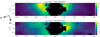 |
Fig. 2 3.3 μm and 3.4 μm band emission maps. Intensities are integrals of the Gaussians related to the bands, as shown in Fig. 1. Positions of the spectra in Fig. 1 are represented by the coloured symbols. |
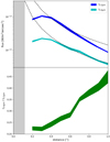 |
Fig. 3 Top panel: I3.3μm (blue) and I3.4μm (cyan) band emission according to the distance to the star. Values are the sum of the integrals of the Gaussians related to each feature and averaged for different distances from the star in 0.1′′ step. Normalised 1∕d2 functions arealso plotted (dotted black lines) for clarity. Bottom panel: I3.4μm∕I3.3μm band ratio (green) according to the distance to the star. The transparent grey box on the left represents the distance up to which the cavity is extended in the POLARIS simulations (~ 0.12′′ or 13 au). |
3.2 VISIR observations
3.2.1 Observations
VISIR observations were performed using the ESO mid-IR instrument VISIR installed on the VLT (Paranal, Chile), equipped with a DRS (former Boeing) 256 × 256 pixels BIB detector. The object was observed in the imaging and spectroscopic modes. It was observed in the aromatic bands at 8.6 and 11.3 μm (pah1 and pah2 filters) and in the adjacent continuum at 10.4 μm. Under good seeing conditions, it provides diffraction-limited imaging and spectroscopy in the N and Q bands, which is 0.3′′ at 10 μm. The spectrometer offers a range in spectral resolution of 150 to 30 000 and it has a pixel-scale of 127 mas pix−1. In order to remove the high atmospheric background, the instrument employs standard chopping and nodding techniques.
The observations were obtained in 2005 as part of the VISIR GTO program on circumstellar disks. The medium-resolution spectroscopic mode of VISIR was used. VISIR offers a choice in slit-width, slit-rotation, and chopping throw. The orientation of the slit was aligned along the major axis of the disk. Chopping and nodding was performed parallel to the slit for all observations. The standard star used for photometric calibration was HD91056 (Cohen et al. 1999).
3.2.2 Results
Figure 4 shows VISIR mid-IR spectra measured at different distances from the central star (up to 1.8′′). These spectra are centred on the 8.6 and 11.3 μm aromatic features, which correspond to aromatic C-H bending in-plane and out-of-plane vibrational modes, respectively (see Table 1).
The 8.6 μm feature is not observed in the spectra at the star location, but its intensity relative to the adjacent continuum increases significantly from 0.5′′ to 1.5′′. At 1.8′′, its intensity relative to the continuum appears to be lower than at 1.5′′. In the 11–12 μm range of the spectra, two features at 11.4 and 11.9 μm, characteristic of crystalline silicates, are clearly detected at the star location and up to a large distance from the star (at least 1.5′′). The emission in the 11.3 μm band relative to the emission in the crystalline silicate band increases significantly between 0.5′′ and 1.5′′. At 1.8′′, weak aromatic and silicate bands appear. We checked that the contribution from the unresolved peak component does not affect the spectra significantly at large distances. This contribution is estimated to be at most 20% at 1.5–1.8′′.
In order to measure the spatial scales of the bands, the VISIR long-slit spectra were Gaussian-fitted following the van Boekel (2004) procedure to obtain the FWHM sizes as a function of wavelength (see Fig. 5). At each wavelength, the spatial profile was adjusted using a 1D Gaussian model. From the Gaussian model, we then derived a FWHM. Figure 5 shows the measured FWHM for HD 100546 and the standard star, and the ratio between HD 100546 and standard star FWHM. The standard star was assumed to reflect the angular resolution response of the atmosphere combined with the telescope or instrument. The FWHM of the spatially resolved spectrum of HD 100546 is systematically increased in the aromatic bands. The 11.3 μm has a larger FWHM than that of 8.6 μm. The 7.7 μm appears even more extended, although we only see the rise. The FWHM of HD 100546 is also larger at the 11.9 μm crystalline silicate feature than the adjacent continuum. No particular features are present at 11.4 μm, but it is blended with the aromatic 11.3 μm band. The FWHM increase in the crystalline band may suggest nanosilicates that are warm far away from the star.
Figure 6 shows the spatial emission profiles in the VISIR filters centred on the aromatic bands at 8.6 and 11.3 μm and on the 10.4 μm continuum, and the band-to-continuum ratios, depending on the distance from the star. We note that the emission profiles in the VISIR filters are not continuum-subtracted, which is different from Fig. 3, showing the fluxes in the bands. Figure 6 shows that the emission centred on the bands and on the continuum is spatially extended. The two aromatic band-to-continuum ratios increase with distance from the star up to 1′′ (~ 100 au) and are constantat a larger distances. The low ratio values closer to the star are mostly due to the increase in the thermal emission of the larger grainsat thermal equilibrium, the emission of which peaks at shorter wavelength when the UV flux increases. Up to a distance of 0.2–0.3′′ (or ~ 20−30 au) from the star where 106 ≲ G0 ≲ 107, sub-micron grains can reach an equilibrium temperature of ~300 K and thus strongly emit in the 10 μm range. On the other hand, the aromatic band profiles decrease slightly faster than a 1∕d2 law (dashed linein Fig. 6), showing that emission in the two bands does not simply scale linearly with G0. This behaviour is expected when emission is dominated by a single population of stochastically heated grains. This means that the emissionmight be due to a mix of the contributions of different nanograin populations, for instance, extremely small to large nanoparticles. As a consequence, the large nanoparticles reach thermal equilibrium for the high G0 > 104 values at the disk surface and thus modify the scaling of their mid-IR emission spectrum (see Sect. 4 for details). However, near the star, the emission profiles are dominated by the thermal hot grain emission alone.
These observations also indicate that the mid-IR aromatic features are spatially more extended than the 3.3 μm aromatic and 3.4 μm aliphatic ones (Sect. 3.1.3). The lower energy aromatic bands (at 8.6 and 11.3 μm) are expected to come mostly from the outer disk region (e.g. Habart et al. 2004), whereas the bands with the highest energy (at 3.3 μm) is expected to be least extended.
In order to probe the properties of the emitting particles, the intensity band ratios I11.3 μm∕I8.6 μm might be compared, which are particularly sensitive to their ionisation state, and the I11.3 μm∕I3.3 μm, mostly depending on their size (e.g. Croiset et al. 2016). Nevertheless, from 0.5 to 1.5′′, where the aromatic bands are detected, an analysis like this with our NaCo and VISIR data would be difficult. The 8.6 μm band is partly hidden by the strong continuum, whereas the 11.3 μm band is blended with the crystalline silicate feature at 11.4 μm (see Fig. 4). This analysis is therefore beyond the scope of this study, but will be of prime interest when observations with a high signal-to-noise ratio with the James Webb Space Telescope (JWST) will become available. In particular, the emission at 8.6 and 3.3 μm will be detectable in the outer disk regions.
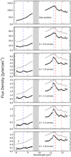 |
Fig. 4 VISIR observed spectra in HD 100546 extracted at different angular distances (0, 0.5, 1.0, 1.2, 1.5, and 1.8″). The grey region delimits the telluric ozone absorption feature. The corresponding grating set-up has not been recorded at that position because of the usual poor quality of the data. A rescaled or offset star position spectrum is repeated (light grey) in all panels to serve as a reference. The positions of the aromatic (blue) andcrystalline forsterite (red) main features in VISIR observation range are overplotted. The typical ± 3σ error derived from background noise is shown in the lower panel. |
Band centre (λ0, ν0) and FWHM variations in laboratory experiments.
4 Disk modelling with THEMIS and POLARIS
4.1 THEMIS dust model
The heterogeneous dust evolution model for interstellar solids (THEMIS1) is an evolutionary core-mantle dust model designed to allow variations in the dust structure, composition, and size according to the local density and radiation field (Jones et al. 2013, 2014, 2017; Bocchio et al. 2014; Köhler et al. 2015). THEMIS has been used before to analyse far-IR to submillimeter observations of the diffuse and dense ISM (e.g. Ysard et al. 2015, 2016), near-IR PPD observations (Boutéraon et al. 2019), and near-IR to submillimeter observations of nearby galaxies (Chastenet et al. 2017; Viaene et al. 2019).
In the following, unless otherwise stated, we use the dust composition and size distribution of the THEMIS diffuse-ISM dust defined by Jones et al. (2013) and Köhler et al. (2014) (Table 2). It consists of three dust populations: a first made of small hydrogenated amorphous carbon nanoparticles (< 20 nm, a-C); a second of larger carbonaceous grains with an hydrogen-rich core surrounded by a 20 nm thick aromatic-rich mantle (a-C:H/a-C); and a third of large amorphous silicate grains of which 10% of the volume is occupied by metallic nano-inclusions of Fe and FeS (a-Sil/a-C). In addition, these silicate cores are surrounded by a 5 nm thick a-C mantle. We therefore consider diffuse-ISM like grains with radius a ≲ 1 μm. At the disk surface, these small grains absorb most of the stellar UV/visible light and dominate the emission in the near- to mid-IR, therefore this is expected to provide a consistent modelling of the NaCo and VISIR observations of HD 100546.
In THEMIS, the population of carbon grains a-C with sizes from 0.4 to 20 nm has continuous size-dependent optical properties and a continuous size distribution. This is different from most dust models (e.g. Desert et al. 1990; Draine & Li 2001; Compiègne et al. 2011).
The grain structure and optical properties were therefore calculated by considering their composition and size, and the resulting spectra are directly relationed to these properties. In order to facilitate comparison with previous models and studies, we distinguish three sub-populations of a-C grains:
-
a-C1: a-C nanoparticles with a ≤ 0.7 nm, which would be equivalent to the smallest PAH grains in Desert et al. (1990), Draine & Li (2001) and Compiègne et al. (2011) and represent ~10% of the mass for all models;
-
a-C2: a-C with 0.7 < a ≤ 1.5 nm, which would be equivalent to the largest PAHs in Desert et al. (1990), Draine & Li (2001) and Compiègne et al. (2011);
-
very small grains (VSG): larger a-C particles with a > 1.5 nm, which would be equivalent to the VSG as defined in Desert et al. (1990), the smallest carbon grains with graphite optical properties in Draine & Li (2001), and the small amorphous carbon grains (SamC) in Compiègne et al. (2011).
The dust mass fraction of each THEMIS dust population and a-C sub-population, that is, the population dust mass MX to the total dust mass Mtotal ratio, qX = MX∕Mtotal are, qa-C1 ~ 10%, qa-C2 ~ 7%, qVSG ~ 6%, qa-C:H/a-C ~ 8% and qa-Sil/a-C ~ 69%.
Finally, for simplicity, we considered only amorphous silicate grains in our model, while several signatures from crystalline silicates have clearly been observed towards HD 100546, as shown in Fig. 4 and in previous studies (e.g. Malfait et al. 1998; Bouwman et al. 2003; Sturm et al. 2010). However, this assumption does not affect our results because we focused on the spatial distribution of the nanocarbon grain emission features and did not analyse the band profiles in detail.
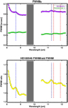 |
Fig. 5 Upper panel: measured FWHM in VISIR long-slit spectra. The ozone atmospheric absorption band is delimited by the grey shaded area. The positions of aromatic (blue) and silicate crystalline (red) main features are shown as dashed lines. The estimated 3 σ error on the FWHM is 2.5 10−3″. The purple points are the measures for HD 100546. The same reference star (HD 91056, green points) as was used for photometriccalibration was used and is assumed to reflect the angular resolution response of the atmosphere combined to the telescope or instrument. Bottom panel: ratio between HD 100546 and standard star FWHM shown in the upper panel. The raw ratio obtained by crude division of the FWHMs was smoothed it with a three-pixel-wide boxcar having the spectral width of the actual spectral sampling in order to reduce pixel-to-pixel irregularities. The estimated 3σ error on the ratio is about 1.2% (~0.02). |
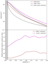 |
Fig. 6 Top panel: 8.6 μm (brown) and 11.3 μm (magenta) aromatic emission bands and 10.4 μm (black) continuum emission plotted according to the distance to the star. The 1∕d2 function is also plotted (black dotted). Bottom panel: 8.6 μm/10.4 μm and 11.3 μm/10.4 μm band ratios plotted according the distance to the star. The transparent grey box on the left represents the distance up to which the cavity is extended in POLARIS simulations, ~ 0.12′′ (13 au). At large distances, the variations in the band-to-continuum ratios are not significant. The error bars on the band-to-continuum ratio are about 5%. |
4.2 POLARIS radiative transfer code
In order to analyse the NaCo and VISIR data with THEMIS, we applied the three-dimensional continuum radiative transfer code POLARIS (Reissl et al. 2016; Brauer et al. 2017). It solves the radiative transfer problem self-consistently with the Monte Carlo method. The main applications of POLARIS are the analysis of magnetic fields by simulating polarised emission of elongated aligned dust grains and the Zeeman splitting of spectral lines. However, recent developments added circumstellar disk modelling as a new main application to POLARIS (e.g. Brauer et al. 2019). For instance, this includes the consideration of complex structures and varying dust grain properties in circumstellar disks and the stochastic heating of nanometre-sized dust grains. We used POLARIS to calculate the spatial dust temperaturedistribution, emission maps, and spectral energy distributions based on the thermal emission of dust grains, the stochastic heating of nanometre-sized dust grains and the stellar emission scattered by dust grains. The code is published on the POLARIS homepage2. For reference, the simulations in this study were performed with version 4.02. of POLARIS.
Our theoretical model of the circumstellar disk consists of a pre-main-sequence star in the centre that is surrounded by an azimuthally symmetric density distribution. The star is characterised by its effective temperature Tstar = 10 500 K and luminosity Lstar = 32 L⊙. For the disk density, we considered a distribution with a radial decrease based on Hayashi (1981) for the minimum mass solar nebula. Combined with a vertical distribution due to hydrostatic equilibrium similar to Shakura & Sunyaev (1973), we obtain the following equation:
![\begin{equation*} \rho_{\text{disk}}=\rho_0 \left(\frac{R_{\text{ref}}}{r} \right)^{a} \exp\left(-\frac{1}{2}\left[\frac{z}{H(r)}\right]^2 \right).\end{equation*}](/articles/aa/full_html/2021/05/aa36388-19/aa36388-19-eq1.png) (1)
(1)
Here, r is the radial distance from the central star in the disk midplane, z is the distance from the midplane of the disk, Rref is a reference radius, and H(r) is the scale height. The density ρ0 is derived from the disk mass. The scale height H(r) is a function of r as follows:
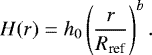 (2)
(2)
The parameters a and b set the radial density profile and the disk flaring, respectively. h0 is the scale height at the characteristic radius Rref = 100 au. Benisty et al. (2010) found a scale height of 10 au at a distance of 100 au for their best disk model around HD 100546, which is equivalent to a flaring angle of 7°. In their model, they assumed a standard flaring index (b = 1.125). Avenhaus et al. (2014) suggested that the disk might be more strongly flared in the outer regions. In our model, we considered a scale height of 10 au at 100 au, similar to Benisty et al. (2010). For the disk flaring b, we assumed b = 9∕7 ~ 1.28, as expected from hydrostatic radiative equilibrium models of passive flared disks (Chiang & Goldreich 1997). The extent of the disk is constrained by the inner radius Rin and outer radius Rout. Following previous studies on HD 100546 discussed in Sect. 2, we considered a disk model with an inner radius of 0.2 au, an outer radius of 350 au, and a cavity between 5 and 13 au (e.g. Bouwman et al. 2003; Brittain et al. 2009; Benisty et al. 2010; Tatulli et al. 2011; Mulders et al. 2013; Panić et al. 2014; Garufi et al. 2016; Follette et al. 2017). Moreover, the inclination of the disk was taken to be equal to 42° (Ardila et al. 2007). An overviewof the assumed parameters of our disk model can be found in Table 3. In the model, we assumed a dust-to-gas mass ratio of Mdust∕MH ~ 7 × 10⁻⁴, which is ten times lower than the standard THEMIS model for diffuse ISM.
The dust-to-gas mass ratio is lower than common literature values (e.g. ~ 0.01), but we considered only the small grains with a ≲ 5 μm in our simulations, while a significant amount of the mass is present in larger grains due to grain growth in disks. However, because the disk is optically thick in the NaCo and VISIR wavelength range, the predicted dust emission profiles are not sensitive to the not-included larger grains, but rather to the relative mass fraction between the different nanometer- and micron-sized grain populations.
Standard THEMIS model parameters as described in Jones et al. (2017).
Parameters of the circumstellar disk model.
4.3 Model results
4.3.1 Physical conditions in the upper surface layers
Figure 7 shows maps of the temperature distribution of large a-C:H/a-C at thermal equilibrium, and of the hydrogen density nH, radiation field intensity G0, and G0∕nH ratio distributions from our disk model. The black lines correspond to 25, 50, and 75% of the total emission at 3.3 μm seen from the top. The emission at 3.3 μm is completely dominated by the upper disk layers due to the high optical depth of the model disk.
Figure 8 presents G0, nH, and G0 ∕nH according to the distance to the star for the disk layers where 25–75% of the total emission at 3.3 μm are seen by the observer. The radiation field G0, which varies as 1/d2, decreases by a factor of about 300 from 20 au to 350 au, with a minimum value slightly lower than 104 at 350 au. The gas density nH decreases by a factor of 100 from 20 to 350 au, with a minimum value of ~ 2 × 106 cm−3 at 350 au. Then, as both G0 and nH decrease with the distance, the G0∕nH ratio does not vary much to first order in the disk layer from which most of the a-C band emission comes. The G0 ∕nH ratio decreases by a factor 3 from ~0.018 at 20 au to ~0.006 at 100 au and remains roughly constant up to 350 au.
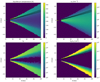 |
Fig. 7 Vertical cuts through the model disk from our POLARIS simulation. The cuts show the temperature (K) distribution of large a-C(:H)/a-C at thermal equilibrium (top left), the hydrogen density nH (cm−3) distribution (top right), the radiation field intensity G0 (bottom left), and the G0∕nH (cm3) ratio (bottom right) of the two previous maps. The black lines correspond to 25, 50, and 75% of the total emission at 3.3 μm seen from the top. The white area in the two lower panels arises because G0 is not defined in the most median parts of the disk because UV radiation does not penetrate them. |
4.3.2 Predicted spectra between 3 and 20 μm
We present the spectra between 3 and 20 μm calculated for the disk model using POLARIS and THEMIS as a function of the distance from the star from 1 to 100 au (see Fig. 9). Predicted spectra are different in the inner and outer disk parts, as expected. In order to facilitate the analysis of the predicted spectra based on THEMIS and DustEM calculations, Fig. 10 shows the emission of each dust sub-population between 3 and 14 μm for several distances to the star.
Figure 10 shows that between 3 and 4 μm, the emission in the aromatic and aliphatic bands is highly dominated by the smallest a-C nanoparticles (a-C1 and a-C2) and the contribution of the larger VSG grains is negligible (a > 1.5 nm). When the radiation field intensity G0 decreases, only the emission due to the smallest a-C nanoparticles, a-C1, remains. At large distance from the star, both the continuum and band emissions are due to these extremely small nanoparticles (a < 0.7 nm). For high G0 values, the contribution of large silicates and VSG grains is significant in the VISIR 8.6 μm bandpass. When the radiation field intensity G0 decreases, the band emission from ~6 to 9 μm is due both to a-C1 and a-C2 amorphous carbon nanoparticles. The shape of the 11.3 μm band is strongly affected by the emission of large silicates for high G0 values. When the radiation field intensity G0 decreases, the band emission is dominated by a-C nanoparticles emission, regardless of their sizes (a-C1, a-C2, or VSG).
All aromatic bands are thus due to different combinations of grain sub-populations with a high dependence on the intensity of the radiation field. The 3.3 μm band is due to a-C1 at both at low and high G0. The 8.6 μm band is due to a-C1 and a-C2 at low G0, and a-C1, a-C2, VSG and a-Sil/a-C at high G0. The 11.3 μm band is sue to a-C1 and a-C2 at low G0, a-C1 and a-Sil/a-C at high G0. At the 10.4 μm continuum, the emission is a mix of the contribution of all grain populations except for the smallest G0. For G0 = 2 × 10⁶ (equivalent to a distance of 20 au), large silicates contribute ~75%, and both large carbonaceous a-C:H/a-C and VSG grains contribute ~ 10%. For G0 = 2 × 10⁵ (75 au), both large silicates and VSG grains contribute >30%, a-C:H/a-C grains ~15%, a-C2 ~10%, and a-C1 ~5%. For G0 = 2 × 10⁴ (200 au), VSG contribute ~45%, a-C2 ~ 30%, and a-C1, a-C:H/a-C, and silicates ~10% or less. However, it should be noted that the SEDs presented in Fig. 10 do not take the scattered light into account. In our POLARIS simulations, this scattered light can make up about half of the continuum in the near-IR but is negligible at wavelengths larger than 10 μm. This is true for the characteristic silicate grain size of 140 nm presented in our model (see Table 2) and remains valid for sizes up to ~1 mm.
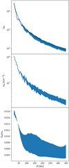 |
Fig. 8 G0, nH, and G0 ∕nH according to distances to the star for the model. G0 is the average of G0 values between 25 and 75% of the total emission at 3.3 μm seen by the observer (Fig. 7, top panel). Idem for nH (middle panel) and G0/nH (bottom panel). The width of the line is for the standard dispersion of the values. 1∕d2 (dotted black line) is also plotted in the top panel. |
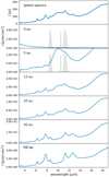 |
Fig. 9 IR emission POLARIS spectra between 3 and 20 μm. Global (Jy) (top panel) and individual emission spectra (Jy arcsec−2) are plotted from 1 au (second panel) to 100 au (bottom) from the star. VISIR filters are also plotted (grey). |
5 Comparison between model predictions and observations
In this section we compare the model predictions to the observations. We first discuss the predicted and the observed integrated fluxes in thenanodust bands over the disk, and then compare their predicted and observed spatial emission profiles by NaCo and VISIR as a function of the distance to the central star.
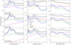 |
Fig. 10 Grain population emission in the IR: tTotal emission (black), a-C1 (blue), a-C2 (green), VSG (magenta),a-C:H/a-C (grey dot), and a-Sil/a-C (orange dot). Left panels: NaCo range between 3 and 4 μm. Middle and right panels: range covered by VISIR filters: 8.6, 10.4, and 11.3 μm. From top to bottom: decrease in G0 values, which are 2 × 10⁶, 2 × 10⁵, and 2 × 10⁴. The corresponding distances to the star are 20, 75, and 200 au, respectively. The distance and G0 ∕nH are derived from Fig. 8. |
5.1 Predicted and observed integrated fluxes in the bands over the disk
Figure 11 presents the global spectra over the disk between 3 and 20 μm as observed and as predicted by the model. The predicted spectrum reproduces the overall shape of the observed spectrum with the main bands. Nevertheless, the predicted flux is overall higher than that observed by a factor of 2–4. Table 4 presents the integrated fluxes of the aromatic and aliphatic features at 3.3 and 3.4 μm, and the aromatic features at 6.2 and 8.6 μm, as observed and as predicted by the model over the disk. For the observation of the aromatic bands, we took the fluxes as derived from the ISO spectrum (Van Kerckhoven 2002). We did not include the 11.3 μm band because it is blended with strong silicate emission. For the observation of the aliphatic band, we took the fluxes as derived from the NaCo spectrum over the disk. The model overestimates the integrated fluxes in the aromatic band at 3.3 μm by a factor of 4. This difference is mainly caused by the overestimation in the model of the internal regions of the disk (r < 40 au), as suggested by the comparison of the observed and predicted profiles (see next section). The band at 3.3 μm reaches 50% of its flux at a radius of r < 20−30 au (0.18–0.27′′). The aliphatic-to-aromatic band ratio  observed over the disk is well reproduced by the models within 20%. The model overestimates the integrated flux in the band at 6.2 and 8.6 μm by a factor of 2.5. This difference is also mainly due to the model overestimation in the internal regions of the disk. The difference with the observations is smaller than for the 3.3 μm because these bands at longer wavelength come from more external regions. The band at 8.6 μm reaches 50% of its flux at a radius of r < 60 au (0.54′′). The model overestimation in the external regions of the disk can also contribute, but in weaker ways.
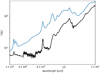 |
Fig. 11 Global spectra (Jy) between 3 and 20 μm as observed by ISO (black) and as predicted by the model (blue). |
5.2 Predicted spatial distribution compared to NaCo data
Figure 12 presents the predicted and the observed spatial emission profiles of the aromatic and aliphatic bands at 3.3 and 3.4 μm as a function of the distance to the central star. The predicted cubes were convolved by a Gaussian with a FWHM of 0.1′′. The same decomposition with ROHSA was applied to the models to compare them with the observations. To do so, a mask must be used aroundthe central star because of the high magnitude gradient between on-star spectra and spectra farther away from the star.
The simulated band emission roughly reproduces the behaviour of the observed profiles but overestimates the observation of the 3.3 μm feature at 1′′ by a factor of 2. Furthermore, close to the inner rim of the outer disk (between 0.2 and 0.4′′ or 20 and 40 au), the model does not reproduce the observed plateau and overestimates the intensity by a factor of 2–10. In this region, the observed emission is flat and no longer varies with G0. This could be due to disk structure effects, such as the shadow of the inner edge of the outer disk due to a puffed-up inner rim, or changes in the properties of the smallest nanoparticles, such as a decrease in the a-C1 mass fraction.
Integrated fluxes of the aromatic and aliphatic features as observed and as predicted by the model over the disk.
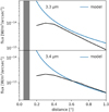 |
Fig. 12 I3.3μm (top panel) and I3.4μm (bottom panel) as observed by NaCo (black) and as predicted by the model (blue). The fluxes are the sum of the integrals of the Gaussians related to each feature and averaged for different distances from the star in 0.1′′ steps. The transparent grey box on the left represents the distance up to which the cavity is extended in the POLARIS simulations: ~0.12′′ or 13 au). The models were convolved with a 0.1′′ Gaussian. Amask must be used around the central star because of the high magnitude gradient between on-star spectra and others. |
5.3 Predicted spatial distribution compared to VISIR data
Figure 13 presents the predicted and the observed spatial emission profiles in the VISIR bands centred at 8.6 and 11.3 μm and in the 10.4 μm continuum as a function of the distance to the central star. As in the observed emission profiles, the continuum was not subtracted from the model profiles at 8.6 and 11.3 μm. The predicted cubes were convolved by a Gaussian with a FWHM of 0.3′′.
In the predicted emission profiles, two regimes appear: thermal emission dominates until 0.5′′ and then stochastically heated dust emission as 1∕d2 for d > 0.5′′ (50 au), which corresponds to the distance where the model spectra at 10 μm are mostly due to emission of nanoparticles. Between 50 and 200 au, the 10 μm continuum emission is mostly due to the VSG (a ~ 10 nm) and a-C2 (a ~ 1 nm) populations, while the 8.6 and 11.3 μm emission bands are mostly due to a-C1 and a-C2. In term of heating regimes the a-C1 are stochastically heated. The a-C2 reach thermal equilibrium for G0 of about 105. Then for G0 = 104−105, they have an intermediate behaviour. The VSG are at thermal equilibrium (whatever the G0).
The observed spatial emission profile is fairly well reproduced by our model. Nevertheless, the model overestimates the flux in the inner regions, and the two emission mechanism regimes appear much less pronounced in the observed spatial emission profiles. At large distance, the observed profile does not scale with 1∕d2 but appears slightly steeper, as expected if thermal equilibrium emission cannot be neglected. Because we did not try to fit the VISIR data with our simulations, these discrepancies could be explained by the parameter choices we made. A change in the flux level could be obtained by increasing the mass fraction of the VSG and a-C2 populations for which we have no a priori observational constraints. The NaCo data can only constrain the a-C1 population mass fraction (see Sect. 3.1.3).
6 Discussion
6.1 Aliphatic-to-aromatic band ratio as a function of the G0 /nH ratio
In Sect. 3 we showed that the aliphatic-to-aromatic band ratio decreases when the central star is approached.This may reflect the processing of the hydrocarbon grains a-C:H by UV photons. Laboratory experimentshave shown that aliphatic CH bonds are more easily photo-destroyed than aromatic CH bonds (e.g. Muñoz Caro et al. 2001; Mennella et al. 2001; Gadallah et al. 2012). Consequently, a decrease in the aliphatic-to-aromatic band ratio in the inner disk part is expected because the nanoparticles are more strongly irradiated. Nevertheless, we must underline that the aliphatic-to-aromatic band ratio remains quite high, about ~ 0.2−0.25, at 0.2′′ from the central star, while the UV field strength is very high, G0 ~ 2 × 10⁶ (see Sect. 4). According to Jones et al. (2014), the a-C(:H) photo-processing timescale τUV, pd can analytically be expressed as
![\begin{equation*} \tau_{\textrm{UV, pd}}(a, G_0) = \frac{10^4}{G_0} \left[ 2.7 + \frac{6.5}{(a [\textrm{nm}])^{1.4}} + 0.04 a[\textrm{nm}]^{1.3}\right] [\textrm{yr}], \end{equation*}](/articles/aa/full_html/2021/05/aa36388-19/aa36388-19-eq4.png) (3)
(3)
which means that the dehydrogenation timescale is expected to be shorter than about two months for the three populations of a-C(:H) nano-particles. However, the emission in the 3–4 μm range depends not only on the UV flux, but also on the (re-)hydrogenation rate, which in turn depends on the gas density. Thus, the observation of an aliphatic-to-aromatic band ratio that varies little may suggest a recent exposure of the carriers to the radiation field (by a continuous local replenishment at the disk surface) before their destruction or conversion, and that the G0 ∕nH ratio may be a better parameter to consider than the UV field strength alone. Figure 14 shows the average spatial profile of the aliphatic-to-aromatic band ratio, I3.4 μm∕I3.3 μm, according to the G0∕nH calculated with POLARIS in the disk surface zone from which most of the band emission originates (see Fig. 8 in Sect. 4). We find that the aliphatic-to-aromatic band ratio decreases from ~ 0.45 to 0.22 for an increase in the G0∕nH ratio from ~ 0.008 to 0.018 as computed from model 1. This decrease for this range of G0∕nH values appears consistent with previous studies based on spatially resolved 3–4 μm spectra towards extended photodissociation regions (Pilleri et al. 2015) and other PPDs (Boutéraon et al. 2019).
In order to interpret the dependence of the I3.4 μm∕I3.3 μm ratio as function of the local physical conditions (G0, nH) more accurately, a more detailed modelling study is needed. Depending on the photon-grain interaction site and on the photon energy, heating, H atom loss, rehydrogenation, and fragmentation should be characterised to determine the time-dependent size distribution and composition as a function of G0 and nH. This is beyond the scope of the present study, however.
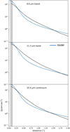 |
Fig. 13 8.6 μm (top panel), 11.3 μm (middle panel), and 10.4 μm (bottom panel) VISIR bands (grey) vs. the model. The predicted profiles were convolved with a Gaussian of 0.3′′ similar to the spatial resolution ofVISIR and integrated using VISIR filters to compare to the observations. The transparent grey box on the left represents the distance up to which the cavity is extended in the POLARIS simulations: ~ 0.12′′ (13 au). |
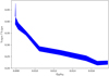 |
Fig. 14 Spatial profile of the aliphatic-to-aromatic band ratio, I3.4 μm∕I3.3 μm, according to the G0∕nH ratio calculated with POLARIS in the disk surface zone from which most of the band emission originates. The highest values of G0∕nH correspond to the regions closest to the star. |
6.2 3–4 μm spectra near the star and spatial distribution of the 3.52 μm band
This work is mostly focused on the aromatic and aliphatic bands at 3.3 and 3.4 μm located between 20 and 100 au from the central star. However, it should be noted that the spectra taken in the inner 20 au of the disk are quite different compared to those from the remaining disk. Over a strong continuum emission due to hot large grains, the NaCo spectra centred on the star (r < 20 au) show a possible faint aromatic band at 3.3 μm and a faint band at 3.52 μm. On the other hand, there is no clear evidence of aliphatic bands at 3.4, 3.43, 3.46, and 3.56 μm. This is in accordance with the analysis of the remaining disk showing that the I3.4 μm∕I3.3 μm ratio decreases when the star is approached. The detection of a faint band at 3.52 μm in the spectra centred on the star also appears to be consistent with the map at 3.52 μm obtained with ROHSA showing a more centrally concentrated emission distribution than the 3.3 and 3.4 μm features (see Fig. A.1).
The 3.52 μm band could be emission from nanodiamonds, as were suggested in the HD 97048 and Elias 1 PPD system, where strong emission features at 3.4–3.5 μm have been detected and are found to be more centrally concentrated than the aromatic emission (Habart et al. 2004; Goto et al. 2009). However, higher angular resolution observations probing the carbon dust features in the innermost regions are needed. The Multi AperTure mid-Infrared SpectroScopic Experiment (MATISSE) instrument has offerered the possibility of performing interferometric observations with a medium spectral resolution in the 3–4 and 8–13 μm domain since 2019. It will teach us about the spatial distribution and dust properties at the scale of 0.1–10 au.
7 Conclusions
We have investigated the nanograin emission in the (pre-)transitional disk HD 100546 by comparing high angular spectroscopic observations with model predictions. We analysed adaptive optics spectroscopic data (VLT/NAOS- CONICA, 3–4 μm, angular resolution 0.1′′) and imaging and spectroscopic data (VLT/VISIR, 8-12 μm, angular resolution 0.3′′). The NaCo spectral cube was decomposed using a tool for hyper-spectral analysis (ROHSA) in order to produce the first emission maps in the aromatic and aliphatic features in the 3–4 μm range. In our modelling, the THEMIS dust model was integrated into the radiative transfer code POLARIS to calculate the thermal and stochastic heating of micro- and nanometric dust grains inside a disk structure. In the THEMIS model, the carbon grains with sizes from 0.4 to 20 nm have continuous size-dependent optical properties and a continuous size distribution, which is different from most dust models. This allowed us to model the sub- and main features characterising bonds between carbon and hydrogen atoms in the 3–4 μm range. These features strongly depend on the grain size distribution and the hydrogen-to-carbon ratio in the grains, depending on their more or less aromatic or aliphatic nature. They also vary with the local environment properties G0 and nH. Our main results derived from both observations and model predictions are summarised belwo.
- 1.
The aromatic and aliphatic features between 3.3 and 3.5 μm are spatially extended. Each band shows a unique morphology.
- 2.
The aliphatic-to-aromatic band ratio, 3.4/3.3, increases with the distance to the star from ~0.2 (at 0.2′′ or 20 au) to ~0.45 (at 1′′ or 100 au). This is in agreement with previous studies and argues for an evolution of the composition of nanomaterials that are more aromatic in the disk parts close to the star, where the UV field (G0) is high.
- 3.
The model predicts that the aromatic and aliphatic bands are due to different combinations of grain sub-populations with a high dependence on the intensity of the UV radiation field (G0). The 3.3 and 3.4 μm features are mainly due the extremely small nanoparticles with a ≤ 0.7 nm both at low and high G0. On the other hand, the 8.6 and 11.3 μm features are mainly due to the larger nanoparticles with a ≤1.5 nm at low G0, and a mix of the contribution of several grain populations at high G0. The 10.4 μm continuum is mainly due to the sub-micron grains near the star, while at large distance, the largest nano-particles (a ≥1.5 nm) contribute ~50%, and nano-particles with a ≤1.5 nm and a ≤ 0.7 nm contribute ~40% and ~10, respectively.
- 4.
The observed continuum emission at 10 μm is spatially extended, as in the bands at 8.6 and 11.3 μm. This is in agreement with the model, which predicts that at large distance, the continuum emission is mainly caused by nanoparticles of extremely small to larger sizes.
- 5.
In the observed spectra in the 8–12 μm range, several aromatic and crystalline silicates features are detected up to a large distance (at least 1.5′′). The emission in the aromatic bands increases between 0.5′′ and 1.5′′. The crystalline features at large distance might suggest nanosilicates.
- 6.
We investigated a disk model that reproduces the spatial emission profiles of the 3.3 and 3.4 μm bands well, except for the inner 20–40 au, where the observed emission is, unlike the predictions, flat and no longer increases with the UV field. The possible explanations are disk structure effects (e.g. shadow of the inner edge of the outer disk) or a decrease in the mass fraction in the nanoparticles with a ≤ 0.7 nm mainly responsible for the 3.3 and 3.4 μm features. The model reproduces the observed spatial emission profiles in the mid-IR at 8.6, 10.4 and 11.3 μm fairly well.
Our understanding of the evolution of carbonaceous nanograins in PPDs is expected to make significant progress by constraints imposed by upcoming spatially resolved spectroscopic observations of the carbon nanograins in protoplanetary disks with the VLTI/MATISSE and JWST. Interferometric observations might be used to constrain the spatial distribution and properties of carbonaceous material in the terrestrial planet forming region. On the other hand, observations with the JWST covering a complete spectral domain between 0.6 and 28 μm will mainly probe the warm gas and small dust content with a spatial resolution of 10–100 au and for distances up to 500 au. Spatially resolved spectroscopy of the sub-features from aromatic/PAHs and aliphatics will be obtained and permit a better identification of the nature of the band carriers and the main processes.
Acknowledgements
This work was based on observations collected at the European Southern Observatory, Chile (ESO proposal number: 075.C-0624(A)), and was supported by P2IO LabEx (ANR-10-LABX-0038) in the framework of the “Investissements d’Avenir” (ANR-11-IDEX-0003-01) managed by the Agence Nationale de la Recherche (ANR, France), P2IO LabEx (A-JWST-01-02-01+LABEXP2IOPDO), and Programme National “Physique et Chimie du Milieu Interstellaire” (PCMI) of CNRS/INSU with INC/INP co-funded by CEA and CNES.
Appendix A ROHSA decomposition
Figure A.1 shows Gaussians related to the main features in the NaCo observations. They are gathered according to their central wavelength and summed (last column). Similarly to Boutéraon et al. (2019), we considered six features related to carbonaceous materials at 3.3, 3.4, 3.43, 3.46, 3.52, and 3.56 μm. Each feature presents a spatially structured distribution.
The 3.52 μm band peaks close to the central regions. As we discuss in Sect. 6.2, this feature is seen close to the star. The 3.43 μm band distribution is quite similarto the 3.52 μm one. These two features are usually attributed to nanodiamonds (Goto et al. 2009).
At about 3.74 μm lies the hydrogen recombination line Pfund 8, which corresponds to a Lorentzian mechanism. In this decomposition, we only used Gaussian functions, therefore two Gaussians are needed to reproduce the signature.
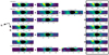 |
Fig. A.1 Main feature maps from the ROHSA decomposition of NaCo data. The last column is the sum of the first columns. Figure 2 showed that several Gaussians are sometimes needed to reproduce the features. |
References
- Acke, B., & van den Ancker, M. E. 2004, A&A, 426, 151 [NASA ADS] [CrossRef] [EDP Sciences] [Google Scholar]
- Acke, B., Bouwman, J., Juhász, A., et al. 2010, ApJ, 718, 558 [NASA ADS] [CrossRef] [Google Scholar]
- Ardila, D. R., Golimowski, D. A., Krist, J. E., et al. 2007, ApJ, 665, 512 [NASA ADS] [CrossRef] [Google Scholar]
- Augereau, J. C., Lagrange, A. M., Mouillet, D., & Ménard, F. 2001, A&A, 365, 78 [NASA ADS] [CrossRef] [EDP Sciences] [Google Scholar]
- Avenhaus, H., Quanz, S. P., Meyer, M. R., et al. 2014, ApJ, 790, 56 [Google Scholar]
- Benisty, M., Tatulli, E., Ménard, F., & Swain, M. R. 2010, A&A, 511, A75 [NASA ADS] [CrossRef] [EDP Sciences] [Google Scholar]
- Boccaletti, A., Pantin, E., Lagrange, A. M., et al. 2013, A&A, 560, A20 [NASA ADS] [CrossRef] [EDP Sciences] [Google Scholar]
- Bocchio, M., Jones, A. P., & Slavin, J. D. 2014, A&A, 570, A32 [NASA ADS] [CrossRef] [EDP Sciences] [Google Scholar]
- Boutéraon, T., Habart, E., Ysard, N., et al. 2019, A&A, 623, A135 [NASA ADS] [CrossRef] [EDP Sciences] [Google Scholar]
- Bouwman, J., de Koter, A., Dominik, C., & Waters, L. B. F. M. 2003, A&A, 401, 577 [NASA ADS] [CrossRef] [EDP Sciences] [Google Scholar]
- Brauer, R., Wolf, S., Reissl, S., & Ober, F. 2017, A&A, 601, A90 [NASA ADS] [CrossRef] [EDP Sciences] [Google Scholar]
- Brauer, R., Pantin, E., Di Folco, E., et al. 2019, A&A, 628, A88 [NASA ADS] [CrossRef] [EDP Sciences] [Google Scholar]
- Brittain, S. D., Najita, J. R., & Carr, J. S. 2009, ApJ, 702, 85 [NASA ADS] [CrossRef] [Google Scholar]
- Brooke, T. Y., Tokunaga, A. T., & Strom, S. E. 1993, AJ, 106, 656 [NASA ADS] [CrossRef] [Google Scholar]
- Carmona, A., van der Plas, G., van den Ancker, M. E., et al. 2011, A&A, 533, A39 [NASA ADS] [CrossRef] [EDP Sciences] [Google Scholar]
- Chastenet, J., Bot, C., Gordon, K. D., et al. 2017, A&A, 601, A55 [NASA ADS] [CrossRef] [EDP Sciences] [Google Scholar]
- Chiang, E. I., & Goldreich, P. 1997, ApJ, 490, 368 [NASA ADS] [CrossRef] [Google Scholar]
- Cohen, M., Walker, R. G., Carter, B., et al. 1999, AJ, 117, 1864 [Google Scholar]
- Compiègne, M., Verstraete, L., Jones, A., et al. 2011, A&A, 525, A103 [NASA ADS] [CrossRef] [EDP Sciences] [Google Scholar]
- Croiset, B. A., Candian, A., Berné, O., & Tielens, A. G. G. M. 2016, A&A, 590, A26 [NASA ADS] [CrossRef] [EDP Sciences] [Google Scholar]
- Currie, T., Cloutier, R., Brittain, S., et al. 2015, ApJ, 814, L27 [Google Scholar]
- Desert, F. X., Boulanger, F., & Puget, J. L. 1990, A&A, 500, 313 [Google Scholar]
- Draine, B. T., & Li, A. 2001, ApJ, 551, 807 [NASA ADS] [CrossRef] [Google Scholar]
- Draine, B. T., & Li, A. 2007, ApJ, 657, 810 [Google Scholar]
- Follette, K. B., Rameau, J., Dong, R., et al. 2017, AJ, 153, 264 [Google Scholar]
- Gadallah, K. A. K., Mutschke, H., & Jäger, C. 2012, A&A, 544, A107 [NASA ADS] [CrossRef] [EDP Sciences] [Google Scholar]
- Gaia Collaboration (Brown, A. G. A., et al.) 2018, A&A, 616, A1 [NASA ADS] [CrossRef] [EDP Sciences] [Google Scholar]
- Garufi, A., Quanz, S. P., Schmid, H. M., et al. 2016, A&A, 588, A8 [NASA ADS] [CrossRef] [EDP Sciences] [Google Scholar]
- Geers, V. C., Pontoppidan, K. M., van Dishoeck, E. F., et al. 2007, A&A, 469, L35 [NASA ADS] [CrossRef] [EDP Sciences] [Google Scholar]
- Gorti, U., & Hollenbach, D. 2008, ApJ, 683, 287 [Google Scholar]
- Goto, M., Henning, T., Kouchi, A., et al. 2009, ApJ, 693, 610 [NASA ADS] [CrossRef] [Google Scholar]
- Grady, C. A., Polomski, E. F., Henning, T., et al. 2001, AJ, 122, 3396 [NASA ADS] [CrossRef] [Google Scholar]
- Grady, C. A., Woodgate, B., Heap, S. R., et al. 2005, ApJ, 620, 470 [Google Scholar]
- Habart, E., Natta, A., & Krügel, E. 2004, A&A, 427, 179 [NASA ADS] [CrossRef] [EDP Sciences] [Google Scholar]
- Habart, E., Natta, A., Testi, L., & Carbillet, M. 2006, A&A, 449, 1067 [NASA ADS] [CrossRef] [EDP Sciences] [Google Scholar]
- Habing, H. J. 1968, Bull. Astron. Inst. Netherlands, 19, 421 [Google Scholar]
- Hayashi, C. 1981, Prog. Theor. Phys. Suppl., 70, 35 [Google Scholar]
- Hu, J. Y., The, P. S., & de Winter, D. 1989, A&A, 208, 213 [Google Scholar]
- Jones, A. P., Fanciullo, L., Köhler, M., et al. 2013, A&A, 558, A62 [NASA ADS] [CrossRef] [EDP Sciences] [Google Scholar]
- Jones, A. P., Ysard, N., Köhler, M., et al. 2014, Faraday Discuss., 168, 313 [Google Scholar]
- Jones, A. P., Köhler, M., Ysard, N., Bocchio, M., & Verstraete, L. 2017, A&A, 602, A46 [NASA ADS] [CrossRef] [EDP Sciences] [Google Scholar]
- Klarmann, L., Benisty, M., Min, M., et al. 2017, A&A, 599, A80 [NASA ADS] [CrossRef] [EDP Sciences] [Google Scholar]
- Kluska, J., Kraus, S., Davies, C. L., et al. 2018, ApJ, 855, 44 [NASA ADS] [CrossRef] [Google Scholar]
- Köhler, M., Jones, A., & Ysard, N. 2014, A&A, 565, L9 [NASA ADS] [CrossRef] [EDP Sciences] [Google Scholar]
- Köhler, M., Ysard, N., & Jones, A. P. 2015, A&A, 579, A15 [NASA ADS] [CrossRef] [EDP Sciences] [Google Scholar]
- Kraus, S., Ireland, M. J., Sitko, M. L., et al. 2013, ApJ, 768, 80 [Google Scholar]
- Lagage, P.-O., Doucet, C., Pantin, E., et al. 2006, Science, 314, 621 [NASA ADS] [CrossRef] [PubMed] [Google Scholar]
- Li, A., & Draine, B. T. 2001, ApJ, 554, 778 [Google Scholar]
- Liu, W. M., Hinz, P. M., Meyer, M. R., et al. 2003, ApJ, 598, L111 [NASA ADS] [CrossRef] [Google Scholar]
- Maaskant, K. M., Honda, M., Waters, L. B. F. M., et al. 2013, A&A, 555, A64 [NASA ADS] [CrossRef] [EDP Sciences] [Google Scholar]
- Malfait, K., Waelkens, C., Waters, L. B. F. M., et al. 1998, A&A, 332, L25 [Google Scholar]
- Marchal, A., Miville-Deschênes, M.-A., Orieux, F., et al. 2019, A&A, 626, A101 [NASA ADS] [CrossRef] [EDP Sciences] [Google Scholar]
- Meeus, G., Waters, L. B. F. M., Bouwman, J., et al. 2001, A&A, 365, 476 [NASA ADS] [CrossRef] [EDP Sciences] [Google Scholar]
- Meeus, G., Montesinos, B., Mendigutía, I., et al. 2012, A&A, 544, A78 [NASA ADS] [CrossRef] [EDP Sciences] [Google Scholar]
- Meeus, G., Salyk, C., Bruderer, S., et al. 2013, A&A, 559, A84 [NASA ADS] [CrossRef] [EDP Sciences] [Google Scholar]
- Mennella, V., Muñoz Caro, G. M., Ruiterkamp, R., et al. 2001, A&A, 367, 355 [NASA ADS] [CrossRef] [EDP Sciences] [Google Scholar]
- Miley, J. M., Panić, O., Haworth, T. J., et al. 2019, MNRAS, 485, 739 [Google Scholar]
- Muñoz Caro, G. M., Ruiterkamp, R., Schutte, W. A., Greenberg, J. M., & Mennella, V. 2001, A&A, 367, 347 [NASA ADS] [CrossRef] [EDP Sciences] [Google Scholar]
- Mulders, G. D., Paardekooper, S.-J., Panić, O., et al. 2013, A&A, 557, A68 [NASA ADS] [CrossRef] [EDP Sciences] [Google Scholar]
- Panić, O., Ratzka, T., Mulders, G. D., et al. 2014, A&A, 562, A101 [NASA ADS] [CrossRef] [EDP Sciences] [Google Scholar]
- Pantin, E., Waelkens, C., & Lagage, P. O. 2000, A&A, 361, L9 [NASA ADS] [Google Scholar]
- Pérez, S., Casassus, S., Hales, A., et al. 2020, ApJ, 889, L24 [Google Scholar]
- Pilleri, P., Joblin, C., Boulanger, F., & Onaka, T. 2015, A&A, 577, A16 [NASA ADS] [CrossRef] [EDP Sciences] [Google Scholar]
- Pineda, J. E., Szulágyi, J., Quanz, S. P., et al. 2019, ApJ, 871, 48 [Google Scholar]
- Quanz, S. P., Amara, A., Meyer, M. R., et al. 2015, ApJ, 807, 64 [Google Scholar]
- Rameau, J., Follette, K. B., Pueyo, L., et al. 2017, AJ, 153, 244 [NASA ADS] [CrossRef] [Google Scholar]
- Reissl, S., Wolf, S., & Brauer, R. 2016, A&A, 593, A87 [NASA ADS] [CrossRef] [EDP Sciences] [Google Scholar]
- Seok, J. Y., & Li, A. 2017, ApJ, 835, 291 [NASA ADS] [CrossRef] [Google Scholar]
- Shakura, N. I., & Sunyaev, R. A. 1973, A&A, 500, 33 [NASA ADS] [Google Scholar]
- Sturm, B., Bouwman, J., Henning, T., et al. 2010, A&A, 518, L129 [NASA ADS] [CrossRef] [EDP Sciences] [Google Scholar]
- Tatulli, E., Benisty, M., Ménard, F., et al. 2011, A&A, 531, A1 [NASA ADS] [CrossRef] [EDP Sciences] [Google Scholar]
- Thi, W. F., Ménard, F., Meeus, G., et al. 2011, A&A, 530, L2 [NASA ADS] [CrossRef] [EDP Sciences] [Google Scholar]
- van Boekel, R., Waters, L. B. F. M., Dominik, C., et al. 2004, A&A, 418, 177 [NASA ADS] [CrossRef] [EDP Sciences] [Google Scholar]
- van Boekel, R. J. H. M. 2004, PhD thesis, University of Amsterdam, The Netherlands [Google Scholar]
- van der Plas, G., van den Ancker, M. E., Acke, B., et al. 2009, A&A, 500, 1137 [NASA ADS] [CrossRef] [EDP Sciences] [Google Scholar]
- Van Kerckhoven, C. 2002, PhD thesis, Institute of Astronomy, Katholieke Universiteit Leuven, Belgium [Google Scholar]
- Viaene, S., Sarzi, M., Zabel, N., et al. 2019, A&A, 622, A89 [NASA ADS] [CrossRef] [EDP Sciences] [Google Scholar]
- Ysard, N., Köhler, M., Jones, A., et al. 2015, A&A, 577, A110 [NASA ADS] [CrossRef] [EDP Sciences] [Google Scholar]
- Ysard, N., Köhler, M., Jones, A., et al. 2016, A&A, 588, A44 [NASA ADS] [CrossRef] [EDP Sciences] [Google Scholar]
All Tables
Integrated fluxes of the aromatic and aliphatic features as observed and as predicted by the model over the disk.
All Figures
|
Fig. 1 Mosaic of near-IR emission spectra of HD 100546 between 3.2 and 3.8 μm. Their location (coloured symbols) is reported in Fig. 2. The result of the decomposition with ROHSA (black) is overplotted on NaCo data (grey). Gaussians related to the 3.3 μm aromatic feature are shown in blue, and those related to the 3.4 μm aliphatic feature in cyan. Other features are plotted in brown. |
| In the text | |
|
Fig. 2 3.3 μm and 3.4 μm band emission maps. Intensities are integrals of the Gaussians related to the bands, as shown in Fig. 1. Positions of the spectra in Fig. 1 are represented by the coloured symbols. |
| In the text | |
|
Fig. 3 Top panel: I3.3μm (blue) and I3.4μm (cyan) band emission according to the distance to the star. Values are the sum of the integrals of the Gaussians related to each feature and averaged for different distances from the star in 0.1′′ step. Normalised 1∕d2 functions arealso plotted (dotted black lines) for clarity. Bottom panel: I3.4μm∕I3.3μm band ratio (green) according to the distance to the star. The transparent grey box on the left represents the distance up to which the cavity is extended in the POLARIS simulations (~ 0.12′′ or 13 au). |
| In the text | |
|
Fig. 4 VISIR observed spectra in HD 100546 extracted at different angular distances (0, 0.5, 1.0, 1.2, 1.5, and 1.8″). The grey region delimits the telluric ozone absorption feature. The corresponding grating set-up has not been recorded at that position because of the usual poor quality of the data. A rescaled or offset star position spectrum is repeated (light grey) in all panels to serve as a reference. The positions of the aromatic (blue) andcrystalline forsterite (red) main features in VISIR observation range are overplotted. The typical ± 3σ error derived from background noise is shown in the lower panel. |
| In the text | |
|
Fig. 5 Upper panel: measured FWHM in VISIR long-slit spectra. The ozone atmospheric absorption band is delimited by the grey shaded area. The positions of aromatic (blue) and silicate crystalline (red) main features are shown as dashed lines. The estimated 3 σ error on the FWHM is 2.5 10−3″. The purple points are the measures for HD 100546. The same reference star (HD 91056, green points) as was used for photometriccalibration was used and is assumed to reflect the angular resolution response of the atmosphere combined to the telescope or instrument. Bottom panel: ratio between HD 100546 and standard star FWHM shown in the upper panel. The raw ratio obtained by crude division of the FWHMs was smoothed it with a three-pixel-wide boxcar having the spectral width of the actual spectral sampling in order to reduce pixel-to-pixel irregularities. The estimated 3σ error on the ratio is about 1.2% (~0.02). |
| In the text | |
|
Fig. 6 Top panel: 8.6 μm (brown) and 11.3 μm (magenta) aromatic emission bands and 10.4 μm (black) continuum emission plotted according to the distance to the star. The 1∕d2 function is also plotted (black dotted). Bottom panel: 8.6 μm/10.4 μm and 11.3 μm/10.4 μm band ratios plotted according the distance to the star. The transparent grey box on the left represents the distance up to which the cavity is extended in POLARIS simulations, ~ 0.12′′ (13 au). At large distances, the variations in the band-to-continuum ratios are not significant. The error bars on the band-to-continuum ratio are about 5%. |
| In the text | |
|
Fig. 7 Vertical cuts through the model disk from our POLARIS simulation. The cuts show the temperature (K) distribution of large a-C(:H)/a-C at thermal equilibrium (top left), the hydrogen density nH (cm−3) distribution (top right), the radiation field intensity G0 (bottom left), and the G0∕nH (cm3) ratio (bottom right) of the two previous maps. The black lines correspond to 25, 50, and 75% of the total emission at 3.3 μm seen from the top. The white area in the two lower panels arises because G0 is not defined in the most median parts of the disk because UV radiation does not penetrate them. |
| In the text | |
|
Fig. 8 G0, nH, and G0 ∕nH according to distances to the star for the model. G0 is the average of G0 values between 25 and 75% of the total emission at 3.3 μm seen by the observer (Fig. 7, top panel). Idem for nH (middle panel) and G0/nH (bottom panel). The width of the line is for the standard dispersion of the values. 1∕d2 (dotted black line) is also plotted in the top panel. |
| In the text | |
|
Fig. 9 IR emission POLARIS spectra between 3 and 20 μm. Global (Jy) (top panel) and individual emission spectra (Jy arcsec−2) are plotted from 1 au (second panel) to 100 au (bottom) from the star. VISIR filters are also plotted (grey). |
| In the text | |
|
Fig. 10 Grain population emission in the IR: tTotal emission (black), a-C1 (blue), a-C2 (green), VSG (magenta),a-C:H/a-C (grey dot), and a-Sil/a-C (orange dot). Left panels: NaCo range between 3 and 4 μm. Middle and right panels: range covered by VISIR filters: 8.6, 10.4, and 11.3 μm. From top to bottom: decrease in G0 values, which are 2 × 10⁶, 2 × 10⁵, and 2 × 10⁴. The corresponding distances to the star are 20, 75, and 200 au, respectively. The distance and G0 ∕nH are derived from Fig. 8. |
| In the text | |
|
Fig. 11 Global spectra (Jy) between 3 and 20 μm as observed by ISO (black) and as predicted by the model (blue). |
| In the text | |
|
Fig. 12 I3.3μm (top panel) and I3.4μm (bottom panel) as observed by NaCo (black) and as predicted by the model (blue). The fluxes are the sum of the integrals of the Gaussians related to each feature and averaged for different distances from the star in 0.1′′ steps. The transparent grey box on the left represents the distance up to which the cavity is extended in the POLARIS simulations: ~0.12′′ or 13 au). The models were convolved with a 0.1′′ Gaussian. Amask must be used around the central star because of the high magnitude gradient between on-star spectra and others. |
| In the text | |
|
Fig. 13 8.6 μm (top panel), 11.3 μm (middle panel), and 10.4 μm (bottom panel) VISIR bands (grey) vs. the model. The predicted profiles were convolved with a Gaussian of 0.3′′ similar to the spatial resolution ofVISIR and integrated using VISIR filters to compare to the observations. The transparent grey box on the left represents the distance up to which the cavity is extended in the POLARIS simulations: ~ 0.12′′ (13 au). |
| In the text | |
|
Fig. 14 Spatial profile of the aliphatic-to-aromatic band ratio, I3.4 μm∕I3.3 μm, according to the G0∕nH ratio calculated with POLARIS in the disk surface zone from which most of the band emission originates. The highest values of G0∕nH correspond to the regions closest to the star. |
| In the text | |
|
Fig. A.1 Main feature maps from the ROHSA decomposition of NaCo data. The last column is the sum of the first columns. Figure 2 showed that several Gaussians are sometimes needed to reproduce the features. |
| In the text | |
Current usage metrics show cumulative count of Article Views (full-text article views including HTML views, PDF and ePub downloads, according to the available data) and Abstracts Views on Vision4Press platform.
Data correspond to usage on the plateform after 2015. The current usage metrics is available 48-96 hours after online publication and is updated daily on week days.
Initial download of the metrics may take a while.