| Issue |
A&A
Volume 645, January 2021
|
|
|---|---|---|
| Article Number | A104 | |
| Number of page(s) | 31 | |
| Section | Cosmology (including clusters of galaxies) | |
| DOI | https://doi.org/10.1051/0004-6361/202039070 | |
| Published online | 22 January 2021 | |
KiDS-1000 cosmology: Cosmic shear constraints and comparison between two point statistics
1
Institute for Astronomy, University of Edinburgh, Royal Observatory, Blackford Hill, Edinburgh EH9 3HJ, UK
e-mail: This email address is being protected from spambots. You need JavaScript enabled to view it.
2
Department of Physics and Astronomy, University College London, Gower Street, London WC1E 6BT, UK
3
Ruhr-University Bochum, Astronomical Institute, German Centre for Cosmological Lensing, Universitätsstr. 150, 44801 Bochum, Germany
4
Department of Astrophysical Sciences, Princeton University, 4 Ivy Lane, Princeton, NJ 08544, USA
5
Center for Theoretical Physics, Polish Academy of Sciences, al. Lotników 32/46, 02-668 Warsaw, Poland
6
Centre for Astrophysics & Supercomputing, Swinburne University of Technology, PO Box 218, Hawthorn, VIC 3122, Australia
7
Kapteyn Astronomical Institute, University of Groningen, PO Box 800, 9700 AV Groningen, The Netherlands
8
Argelander-Institut für Astronomie, Auf dem Hügel 71, 53121 Bonn, Germany
9
INAF – Astronomical Observatory of Capodimonte, Via Moiariello 16, 80131 Napoli, Italy
10
Leiden Observatory, Leiden University, Niels Bohrweg 2, 2333 CA Leiden, The Netherlands
11
Department of Physics, University of Oxford, Denys Wilkinson Building, Keble Road, Oxford OX1 3RH, UK
12
INAF – Osservatorio Astronomico di Padova, via dell’Osservatorio 5, 35122 Padova, Italy
13
Shanghai Astronomical Observatory (SHAO), Nandan Road 80, Shanghai 200030, PR China
14
University of Chinese Academy of Sciences, Beijing 100049, PR China
15
Kapteyn Institute, University of Groningen, PO Box 800, 9700 AV Groningen, The Netherlands
Received:
30
July
2020
Accepted:
12
October
2020
Abstract
We present cosmological constraints from a cosmic shear analysis of the fourth data release of the Kilo-Degree Survey (KiDS-1000), which doubles the survey area with nine-band optical and near-infrared photometry with respect to previous KiDS analyses. Adopting a spatially flat standard cosmological model, we find S8 = σ8(Ωm/0.3)0.5 = 0.759−0.021+0.024 for our fiducial analysis, which is in 3σ tension with the prediction of the Planck Legacy analysis of the cosmic microwave background. We compare our fiducial COSEBIs (Complete Orthogonal Sets of E/B-Integrals) analysis with complementary analyses of the two-point shear correlation function and band power spectra, finding the results to be in excellent agreement. We investigate the sensitivity of all three statistics to a number of measurement, astrophysical, and modelling systematics, finding our S8 constraints to be robust and dominated by statistical errors. Our cosmological analysis of different divisions of the data passes the Bayesian internal consistency tests, with the exception of the second tomographic bin. As this bin encompasses low-redshift galaxies, carrying insignificant levels of cosmological information, we find that our results are unchanged by the inclusion or exclusion of this sample.
Key words: gravitational lensing: weak / methods: observational / cosmology: observations / large-scale structure of Universe / cosmological parameters
© ESO 2021
1. Introduction
In this new era of precision cosmology reliable probes of the key parameters of the standard model, ΛCDM (cold dark matter), are indispensable. The weak gravitational lensing effect that coherently distorts the shapes of galaxy images, commonly referred to as cosmic shear, was hailed as such a tool (Albrecht et al. 2006; Peacock et al. 2006); It directly maps the spatial distribution of all gravitating matter along the line of sight and is therefore sensitive to the amplitude and shape of the matter power spectrum (see Kilbinger 2015, for a review). This makes cosmic shear highly complementary to galaxy clustering, which as a spatially localised probe can trace line-of-sight modes of the matter distribution and localised features like baryon acoustic oscillations, but which suffers from the poorly known connection between the galaxy and matter distribution, known as galaxy bias.
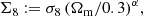
First detected two decades ago (Bacon et al. 2000; Kaiser et al. 2000; Van Waerbeke et al. 2000; Wittman et al. 2000), cosmic shear has since matured into a primary probe in the golden era of galaxy surveys, featuring prominently alongside galaxy clustering in forthcoming experiments like the ESA Euclid mission1 (Laureijs et al. 2011), the Vera C. Rubin Observatory LSST2 (LSST Dark Energy Science Collaboration 2012), and NASA’s Nancy Grace Roman Space Telescope3 (Spergel et al. 2015). To meet the stringent accuracy requirements of these new surveys, all aspects of a cosmic shear analysis have to undergo critical revision and, in many cases, radical improvements. Vital lessons are being learnt by three concurrent surveys, whose analyses are ongoing: the ESO Kilo-Degree Survey4 (KiDS; Kuijken et al. 2015; Hildebrandt et al. 2020a), the Dark Energy Survey5 (DES; Drlica-Wagner et al. 2018; Zuntz et al. 2018), and the Hyper Suprime-Cam Subaru Strategic Program6 (HSC; Aihara et al. 2018; Hikage et al. 2019). The current surveys already have the statistical power to independently test our cosmological standard model, in particular the amplitude of matter density fluctuations which, by convention, is measured via the parameter S8 = σ8 (Ωm/0.3)0.5, where Ωm is the matter density parameter and σ8 is the linear-theory standard deviation of matter density fluctuations in spheres of radius 8 h−1 Mpc.
In this work we present the cosmic shear analysis of the fourth KiDS Data Release (Kuijken et al. 2019), hereafter referred to as KiDS-1000. This data release more than doubles the survey area with respect to the previous KiDS cosmological analyses (Hildebrandt et al. 2017, 2020a). While neither as deep as HSC, once it is completed, nor as wide as the final DES area, KiDS has unique properties that make it competitive in terms of controlling the two major measurement challenges for cosmic shear analyses – the accurate measurement of gravitational shear, resulting from the image distortions imposed by the lensing effect, and the accurate determination of the redshift distribution of the galaxies used in the cosmic shear analysis. As all current cosmic shear analyses can already be considered systematics-limited to some degree (see Mandelbaum 2018 for a recent review of the major challenges), such benefits are likely to directly impact on the final cosmological constraints and could potentially outweigh a larger raw statistical power.
A robust and accurate analysis of cosmic shear data is of paramount importance for testing the concordance of the current standard cosmological model, flat ΛCDM. Currently, the tightest constraints on the parameters of this model come from studies of full-sky comic microwave background (CMB) temperature and polarisation maps. Although these data are primarily sensitive to the physics of the early Universe, given a model, they can make predictions regarding the statistical properties of the structures that formed in the late Universe as well as the current expansion rate. Since the first cosmological analysis of the Planck data (Planck Collaboration XVI 2014), there have been indications of tension between the CMB and cosmic shear results (Heymans et al. 2013) as well as with the Hubble parameter estimated through the distance ladder (Riess et al. 2011).
Recently, there has been a high level of attention towards the ever-growing tension between the estimates of the Hubble parameter from early and late Universe probes (see Verde et al. 2019, for a recent summary). Although not currently as significant, the level of tension in S8 between the probes of the large-scale structures and the Planck results has also been increasing. In particular, the cosmic shear analysis of the first-year data release of DES (DES-Y1, Troxel et al. 2018b), HSC (Hikage et al. 2019) and the KiDS results of Hildebrandt et al. (2020a, KV450) all found values of S8 that are lower than the Planck predictions (Planck Collaboration VI 2020) by around 2σ. Interestingly these results are largely independent, as the images are taken over mostly different patches of the sky and the teams and pipelines analysing them were largely separate7. Therefore, we can assume that the combined analysis of these data sets would result in deviations larger than 2σ. For instance, Joudaki et al. (2020) analysed the combination of DES-Y1 and KV450 data using the KV450 setup and redshift calibrations to find a tension of 2.5σ, and the re-analysis of Asgari et al. (2020) increased the constraining power of DES by including smaller angular scales to find a DES-Y1 and KV450 joint result that is in 3.2σ tension with Planck.
Aside from the importance of the quality of the data, we need to improve the model for a robust analysis. Modelling challenges in cosmic shear prevail especially on small scales where the signal-to-noise ratio is highest and where non-linear structure growth (for example Euclid Collaboration 2019), baryon feedback on the matter distribution (for instance Semboloni et al. 2011), and complex matter-galaxy interactions affecting the intrinsic alignment of galaxies (for example Fortuna et al. 2021) all combine to lead to an uncertainty that is difficult to calibrate and quantify.
It is standard to employ two-point statistics of the gravitational shear as summary statistics, but which choice strikes a balance between the optimal extraction of information and the suppression of observational or modelling systematics? While the KiDS-1000 approach to modelling and inference methodology is discussed in detail in Joachimi et al. (2020), here we focus on the choice of summary statistics and their sensitivity to different systematic and modelling effects.
Two-point statistics of the shear field can be measured in configuration, Fourier or other spaces. In this analysis we consider Complete Orthogonal Sets of E/B-Integrals (COSEBIs; Schneider et al. 2010), band power estimates derived from the correlation functions (Schneider et al. 2002a; Becker & Rozo 2016; van Uitert et al. 2018) and the shear two-point correlation functions (2PCFs). As we discuss in Sect. 2, there are considerable advantages to the former two statistics, since they allow us to avoid scales that are affected by modelling uncertainties, although the latter method has been used in the clear majority of recent cosmic shear analyses (see for example Heymans et al. 2013; Jee et al. 2016; Hildebrandt et al. 2017, 2020a; Joudaki et al. 2017b; Troxel et al. 2018a,b; Wright et al. 2020a; Hamana et al. 2020). With these statistics we connect previous work with this new analysis.
Consistent parameter constraints from a diverse set of summary statistics can add valuable corroboration to cosmological inference. However, care must be taken to accurately quantify the correlation between the different two-point statistics, which could be strong, as they are calculated from the same catalogue, but not perfect, as scales are incorporated and weighted differently. In this work we will apply all summary statistics to the same suite of mock KiDS-1000 data, enabling us to map the expected differences in cosmological constraints. In addition, we triplicate all of our cosmological analyses, including results for 2PCFs, COSEBIs and band powers for all cases.
The KiDS-1000 analysis methodology is discussed in Joachimi et al. (2020, J20), while Giblin et al. (2021, G20) and Hildebrandt et al. (2020b, H20b) detail the construction and calibration of the gravitational shear catalogues and the galaxy redshift distributions used here, respectively. Further KiDS-1000 companion papers include Heymans et al. (2020) who present cosmological constraints from a combined-probe analysis of cosmic shear, galaxy-galaxy lensing and galaxy clustering. Tröster et al. (2020b) extend the cosmological inference from the combined weak lensing and clustering data beyond the spatially flat ΛCDM model considered in the remainder of the KiDS-1000 analyses.
This paper is structured as follows: in Sect. 2 the modelling of the three two-point statistics employed in KiDS-1000 is described. Section 3 provides an overview of the data set and the analysis pipeline. In Sect. 4 the cosmological constraints are presented, including a range of validation tests as well as an assessment of consistency internal to the KiDS data vector and with Planck CMB results, before concluding in Sect. 5. More technical details of the analysis are provided in the appendices. In particular we point the reader to Appendix A where we present constraints on all parameters, Appendix B which details our internal and external consistency tests and Appendix D where we model the impact of the residual constant additive shear biases on our two-point statistics.
2. Methods
We analyse the KiDS-1000 data with three sets of statistics: real-space shear two-point correlation functions (2PCFs), complete orthogonal sets of E/B-integrals (COSEBIs) and band power spectra estimated from 2PCFs (band powers). These statistics are all linear transformations of the observed cosmic shear angular power spectrum, Cϵϵ(ℓ),
 (1)
(1)
where Wx(ℓ) is a weight function that depends on the angular Fourier scale, ℓ, as well as the argument of the statistics, x. The Cϵϵ(ℓ) in turn can be written as a sum of gravitational lensing (G) and intrinsic (I) alignments of galaxies,
 (2)
(2)
The observed cosmic shear signal can in principle consist of E and B-modes. Under the standard cosmological model, however, we do not expect to measure any significant B-modes for surveys such as KiDS8. In this case we can substitute Cϵϵ(ℓ) with CEE, the E-mode angular power spectrum and derive the three terms on the right hand side of Eq. (2) from the matter power spectrum, using a modified Limber approximation (Loverde & Afshordi 2008; Kilbinger et al. 2017),
 (3)
(3)
where X and Y stand for G or I, i and j denote two populations of galaxies, χ is the radial comoving distance and fK(χ) is the comoving angular diameter distance which simplifies to χ for a spatially flat universe. The integral is taken from the observer at χ = 0 to the horizon, χhor. The kernels, WX/Y depend on the redshift distribution of the two populations and their mathematical form can be found in Eqs. (15) and (16) of J20.
It is common practice to divide galaxies based on their estimated photometric redshifts into tomographic bins, which has the advantage of improving the constraining power and reducing the degeneracy between redshift-dependent parameters in a cosmic shear analysis (Hu 1999). In this case i and j in Eq. (3) are the labels for the tomographic bins.
From a theoretical point of view, spherical harmonic measures estimated from a pixelated sky may seem to be the most natural choice of statistics. Such direct power spectrum statistics have seen widespread application in other cosmological probes, most prominently in temperature and polarisation measurements of the cosmic microwave background (CMB: see for example Planck Collaboration V 2020). Analogous statistics, like pixel-based maximum-likelihood quadratic estimators (Brown et al. 2003; Heymans et al. 2005; Lin et al. 2012; Köhlinger et al. 2016, 2017) or pseudo-Cℓ techniques (Hikage et al. 2011, 2019; Becker et al. 2016; Asgari et al. 2018; Alonso et al. 2019), have also been developed for cosmic shear. These measurements are, however, affected directly by masking and finite field effects. Moreover, the significant noise component due to the random intrinsic orientations of galaxy shapes is spread out over all multipoles in harmonic space. For such analyses, these effects have to be either modelled or corrected for. 2PCFs, on the other hand, do not suffer from these limitations, as masking and noise effects do not bias their expectation value, although these effects should be included in their covariance estimation (see Sect. 5 of J20 for a discussion on the importance of each effect). An additional motivation for employing 2PCFs is that measurement systematics are better traced in configuration space.
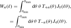
This makes the 2PCFs the current method of choice to be applied to a catalogue of shear estimates. However, considerable disadvantages are revealed in the further stages of the cosmological inference. Due to the very broad kernels linking the 2PCFs to the underlying power spectrum, the analyst has little control over the physical scales entering the likelihood analysis, with undesirable consequences (see Fig. 1). For instance, sensitivity to low-multipoles, where only few independent modes contribute, leads to significant deviations from a Gaussian likelihood for 2PCFs measured on large separations (Schneider & Hartlap 2009; Sellentin et al. 2018), while a fairly wide range of small-scale 2PCF measurements are affected by non-linear modelling uncertainties such as baryon feedback (Asgari et al. 2020). In addition, the 2PCFs mix E-modes, which are expected to carry the cosmological signal, and B-modes, which are influenced by cosmological signals only at a very low level and hence provide a valuable null test for a range of systematics. The 2PCFs are also impacted by ambiguous modes, which cannot be uniquely identified as either E or B-modes.
 |
Fig. 1. Integrands of the transformation between the angular power spectrum and 2PCFs (Eq. (6)), COSEBIs (Eq. (8)) and band powers (Eq. (12)). All integrands are normalised by their maximum value. ξ± results are shown for the maximum and minimum angular separations that are used in our analysis. For COSEBIs we chose n = 1 and n = 5, showing the range of n-modes that we consider. For band powers we show all 8 bins. COSEBIs are defined on the angular range of |
![Mathematical equation: $ [0{{\overset{\prime}{.}}}5, 300{\prime}] $](/articles/aa/full_html/2021/01/aa39070-20/aa39070-20-eq5.gif)
To remedy these shortcomings, we consider two promising alternatives: COSEBIs and band powers. COSEBIs offer a clean separation of E and B-modes over a finite range of available angular scales, with nearly lossless data compression and discrete abscissae as a bonus. Band powers allow for approximate E-/B-mode separation and closely follow the underlying angular power spectra, facilitating intuitive interpretation of the signals. These statistics are, in addition, insensitive to the ambiguous E and B-modes. We will demonstrate that both derived statistics avoid the modelling deficiencies of 2PCFs because of their more compact kernels. We note that direct power spectrum estimators will be applied to KiDS data in forthcoming work (Loureiro et al., in prep.).
In the following subsections we first introduce the 2PCFs and briefly review their measurement method (Sect. 2.1). We then introduce COSEBIs in Sect. 2.2 and summarise the main equations for band power spectra in Sect. 2.3. Finally we compare the scale sensitivity of these statistics in Sect. 2.4.
2.1. Shear two-point correlation functions
The shear two-point correlation functions, ξ± (Kaiser 1992), are formally defined as
 (4)
(4)
where γt is the tangential shear and γ× is the cross component of the shear defined with respect to the line connecting the pair of galaxies (see Bartelmann & Schneider 2001, for details). 2PCFs are functions of the angular separation, θ, between pairs of galaxies whose ellipticities are used to estimate shear. In practice we bin the data into several θ-bins and measure the signal using
![Mathematical equation: $$ \begin{aligned} \hat{\xi }^{(ij)}_\pm (\bar{\theta })=\frac{\sum _{ab} w_a w_b \left[\epsilon ^\mathrm{obs}_{{t},a}\epsilon ^\mathrm{obs}_{{t},b} \pm \epsilon ^\mathrm{obs}_{\times ,a}\epsilon ^\mathrm{obs}_{\times ,b}\right] \Delta ^{(ij)}_{ab}(\bar{\theta }) }{\sum _{ab} w_a w_b (1+m_a)(1+m_b) \Delta ^{(ij)}_{ab}(\bar{\theta }) } , \end{aligned} $$](/articles/aa/full_html/2021/01/aa39070-20/aa39070-20-eq7.gif) (5)
(5)
where  is a function that limits the sums to galaxy pairs of separation within the angular bin labelled by
  and the tomographic bins i and j. A galaxy indexed by a is assigned a weight, wa, based on the precision of its shear estimate. These weights are applied to the observed tangential and cross components of the ellipticity,
  and
and  . Finally, the signal is normalised using the denominator, which takes the measurement biases into account, through an averaged multiplicative bias correction, ma. As the value of m is noisy for a single galaxy, we apply its corresponding correction, averaged over all the galaxies in the (tomographic) sample as shown in Eq. (5). This calibration is needed to correct for residual biases such as the effect of noise on the shear estimates (Melchior & Viola 2012), detection biases (Fenech Conti et al. 2017; Kannawadi et al. 2019) as well as blending of the images of galaxies (Hoekstra et al. 2015).
The 2PCFs are linear combinations of the E and B-mode angular power spectra, CEE/BB(ℓ),
![Mathematical equation: $$ \begin{aligned} \xi _\pm (\theta )&=\int _0^{\infty } \frac{\mathrm{d} \ell \, \ell }{2\pi } {J}_{0/4}(\ell \theta ) \left[C_{\rm EE}(\ell )\pm C_{\rm BB}(\ell )\right], \end{aligned} $$](/articles/aa/full_html/2021/01/aa39070-20/aa39070-20-eq12.gif) (6)
(6)
with Bessel functions of the first kind, J0/4, as their weights9. Since we do not expect a significant B-mode signal of cosmological origin, we can use the significance of the B-modes measured in the data as a null test of residual systematics (see for example Hoekstra 2004; Kilbinger et al. 2013; Asgari et al. 2017, 2019; Hikage et al. 2019; Asgari & Heymans 2019). As a result, this mixing of modes makes ξ± unsuitable for systematic tests that utilise B-modes.
The measured 2PCFs are binned in θ, and we match the binning procedure in their theoretical predictions. The theoretical value of ξ± has been estimated using an effective θ in previous cosmic shear analyses (Hildebrandt et al. 2017; Troxel et al. 2018a,b), although this approximation can result in biases (see Appendix A of Asgari et al. 2019). As the number of pairs of galaxies contributing to ξ± increases with angular separation, the correct method to bin the theory vector is to perform a weighted integral over ξ±(θ) and include the effective number of pairs of galaxies, Npair, as the weight. We employ Npair as measured from the data, which includes all survey effects (see Appendix C.3 of J20). The method used to measure the covariance matrix of ξ± is described in Appendix E of J20.
2.2. COSEBIs
The complete orthogonal sets of E/B-integrals (Schneider et al. 2010) are two-point statistics defined on a finite angular range that cleanly separate all well-defined E and B-modes within that range, emoving any ambiguous modes that cannot be uniquely identified as E or B. COSEBIs form discrete values and can be measured through 2PCFs,
![Mathematical equation: $$ \begin{aligned}&E_n = \frac{1}{2} \int _{\theta _{\rm min}}^{\theta _{\rm max}} \mathrm{d}\theta \,\theta \, [T_{+n}(\theta )\,\xi _+(\theta ) + T_{-n}(\theta )\,\xi _-(\theta )], \\&B_n = \frac{1}{2} \int _{\theta _{\rm min}}^{\theta _{\rm max}}\mathrm{d}\theta \,\theta \, [T_{+n}(\theta )\,\xi _+(\theta ) - T_{-n}(\theta )\,\xi _-(\theta )],\nonumber \end{aligned} $$](/articles/aa/full_html/2021/01/aa39070-20/aa39070-20-eq13.gif) (7)
(7)
where T±n(θ) are filter functions defined for a given angular range, such that θ is bounded by θmin and θmax. Schneider et al. (2010) introduced two families of COSEBIs, linear-COSEBIs for which T±(θ) have nearly linearly spaced oscillations, and also log-COSEBIs with nearly logarithmically spaced oscillations. These COSEBI n-modes are numbered with natural numbers, n, starting from 1, and their filters have n + 1 roots in their range of support (see Fig. 1 of Asgari et al. 2019). Log-COSEBIs provide a more efficient data compression in that the first few n-modes are sufficient to essentially capture the full cosmological information (Asgari et al. 2012). Therefore, we employ log-COSEBIs, which were also used for previous data analyses (see for example Kilbinger et al. 2013; Huff et al. 2014; Asgari et al. 2020).
In practice, to measure COSEBIs accurately, we bin the 2PCFs into fine θ-bins before applying the linear transformation in Eq. (7). The accuracy of the measured COSEBIs depends on the binning of the 2PCFs as well as the n-mode considered. For higher n-modes we need a larger number of bins. As our analysis employs log-COSEBIs, we adopt logarithmic binning of the 2PCFs, which results in a lower number of bins to reach the same accuracy requirement than for a linear binning approach. Previously we used linear binning with a million θ-bins (Asgari et al. 2020). With log-binning we can reduce this number to 4000 θ-bins to reach the same level of accuracy (better than 0.03%), resulting in a speed gain in the measurement (see Appendix A of Asgari et al. 2017, for accuracy tests).
The theoretical prediction for COSEBIs can be found through
 (8)
(8)
where the weight functions, Wn(ℓ), are Hankel transforms of T±(θ) (see Fig. 2 in Asgari et al. 2012),
 (9)
(9)
These weight functions are highly oscillatory, but as we will see in Sect. 2.4, they limit the effective range of support of COSEBIs in ℓ, and as a result they allow for more control over which scales enter the analysis. To measure the covariance matrix of COSEBIs, we follow the formalism in Appendix A of Asgari et al. (2020), but with the updated Npair and ellipticity dispersion, σϵ, definitions that are given in Appendix C of J20. We also include the in-survey non-Gaussian term that was neglected in Asgari et al. (2020), although that term has a negligible effect on the analysis (Barreira et al. 2018).
2.3. Band powers
The formalism for band power spectra is described in detail in J20 (see also Schneider et al. 2002a; van Uitert et al. 2018). Band powers are essentially binned angular power spectra, but estimated through 2PCFs. We can measure band powers, 𝒞E/B,l, via
![Mathematical equation: $$ \begin{aligned} {\mathcal{C} }_{\mathrm{E/B},l} = \frac{\pi }{{\mathcal{N} }_l}\; \int _0^\infty \mathrm{d} \theta \, \theta \; T(\theta ) \left[\xi _+(\theta )\; g_+^l(\theta ) \pm \xi _-(\theta )\; g_-^l(\theta )\right], \end{aligned} $$](/articles/aa/full_html/2021/01/aa39070-20/aa39070-20-eq16.gif) (10)
(10)
where the normalisation, 𝒩l, is defined such that the band powers trace ℓ2C(ℓ) at the logarithmic centre of the bin,
 (11)
(11)
with ℓup, l and ℓlo, l defining the edges of the desired top-hat function for the bin indexed by l. The filter functions,  , are given in Eq. (23) of J20. We note that the integral in Eq. (10) is defined over an infinite range of θ. In practice we cannot measure the 2PCFs over all angular distances, therefore, we need to truncate the integral at both ends. As a result it is impossible to produce perfect top-hat functions in Fourier space (Asgari & Schneider 2015). To reduce the ringing effect caused by the limited range of the 2PCFs we introduced apodisation in the selection function, T(θ), that softens the edges of the top hat (see Eq. (22) of J20). We note that T(θ) in Eq. (10) and T±n(θ) in Eq. (7) are unrelated.
The relation between the band powers and the underlying angular power spectra is given by,
![Mathematical equation: $$ \begin{aligned}&{\mathcal{C} }_{\mathrm{E},l} = \frac{1}{2 {\mathcal{N} }_l} \int _0^\infty \mathrm{d} \ell \, \ell \left[ W^l_{\rm EE}(\ell )\; C_{\rm EE}(\ell ) + W^l_{\rm EB}(\ell )\; C_{\rm BB}(\ell ) \right], \\&{\mathcal{C} }_{\mathrm{B},l} = \frac{1}{2 {\mathcal{N} }_l} \int _0^\infty \mathrm{d} \ell \, \ell \left[ W^l_{\rm BE}(\ell )\; C_{\rm EE}(\ell ) + W^l_{\rm BB}(\ell )\; C_{\rm BB}(\ell )\right],\nonumber \end{aligned} $$](/articles/aa/full_html/2021/01/aa39070-20/aa39070-20-eq19.gif) (12)
(12)
where
![Mathematical equation: $$ \begin{aligned}&W^l_{\rm EE}(\ell ) = W^l_{\rm BB}(\ell ) \\&\qquad \quad = \int _{0}^{\infty } \!\! \mathrm{d} \theta \, \theta \; T(\theta ) \left[{ {J}_0(\ell \theta )\; g_+^l(\theta ) + {J}_4(\ell \theta )\; g_-^l(\theta ) }\right], \nonumber \\&W^l_{\rm EB}(\ell ) = W^l_{\rm BE}(\ell ) \nonumber \\&\qquad \quad = \int _{0}^{\infty } \!\! \mathrm{d} \theta \, \theta \; T(\theta ) \left[{ {J}_0(\ell \theta )\; g_+^l(\theta ) - {J}_4(\ell \theta )\; g_-^l(\theta ) }\right].\nonumber \end{aligned} $$](/articles/aa/full_html/2021/01/aa39070-20/aa39070-20-eq20.gif) (13)
(13)
These weight functions are no longer top hat functions (see Fig. 1), however they allow for the correct transformation of the angular power spectra to band powers that can be compared to the measured values from Eq. (10). Similar to COSEBIs, we need to bin the 2PCFs before measuring the band powers. In this case we find that with 300 logarithmic θ-bins in ![Mathematical equation: $ [0{{\overset{\prime}{.}}}5, 300{\prime}] $](/articles/aa/full_html/2021/01/aa39070-20/aa39070-20-eq21.gif) (with the binning extended on either side to allow for the apodisation) we can reach better than percent level accuracy, which is sufficient for the analysis of KiDS-1000 data. We define 8 logarithmically-spaced band power filters within the ℓ-range of 100–1500. The covariance matrix of band powers is estimated by integrating over the covariance matrix of 2PCFs as described in Appendix E.3 of J20.
(with the binning extended on either side to allow for the apodisation) we can reach better than percent level accuracy, which is sufficient for the analysis of KiDS-1000 data. We define 8 logarithmically-spaced band power filters within the ℓ-range of 100–1500. The covariance matrix of band powers is estimated by integrating over the covariance matrix of 2PCFs as described in Appendix E.3 of J20.
2.4. Scale sensitivity of the two-point statistics
All two-point statistics considered here can be measured using linear combinations of finely binned 2PCFs. We set the full angular range for the measured 2PCFs to ![Mathematical equation: $ \theta\in[0{{\overset{\prime}{.}}}5,300{\prime}] $](/articles/aa/full_html/2021/01/aa39070-20/aa39070-20-eq22.gif) following the previous analysis of KiDS data, based on the extent of the survey and its resolution (Hildebrandt et al. 2017). Hildebrandt et al. (2020a) applied extra θ cuts to their data vector. We apply their lower scale cut on ξ− to remove all θ < 4′, since ξ− for these scales are very sensitive to small physical scales where modelling becomes challenging. For COSEBIs and band powers, however, we use the full range of θ-scales available.
following the previous analysis of KiDS data, based on the extent of the survey and its resolution (Hildebrandt et al. 2017). Hildebrandt et al. (2020a) applied extra θ cuts to their data vector. We apply their lower scale cut on ξ− to remove all θ < 4′, since ξ− for these scales are very sensitive to small physical scales where modelling becomes challenging. For COSEBIs and band powers, however, we use the full range of θ-scales available.
Our three sets of summary statistics place varying weights on different scales. Thus we do not expect them to have the same response to scale-dependent effects. Figure1 compares the integrands of these statistics, over the range that is used in the analysis. All integrands are normalised by their maximum value. The top two panels show results for ξ+ and ξ−, for the smallest and largest θ values that we consider in the analysis. The third panel demonstrates the integrands for the first and the fifth COSEBIs modes, since we only use the first 5 n-modes in our cosmological analysis defined on an angular range of ![Mathematical equation: $ [0{{\overset{\prime}{.}}}5,300{\prime}] $](/articles/aa/full_html/2021/01/aa39070-20/aa39070-20-eq23.gif) . The bottom panel belongs to band powers and shows all of the bands that we use.
. The bottom panel belongs to band powers and shows all of the bands that we use.
The first feature that we can immediately see from Fig. 1, is that both correlation functions show substantial sensitivity to ℓ > 1500. In contrast both COSEBIs and band powers are essentially insensitive to these scales. As a result we expect the 2PCFs to be more sensitive to baryon feedback which becomes more important at smaller physical scales. In addition, ξ+ is sensitive to scales below ℓ of about 10. Contributions from these scales can produce non-Gaussian distributions due to the small number of large-scale modes that enter the survey. Figure 17 of J20 compares the distributions of ξ+ and band powers in the SALMO10 simulations, which contain all KiDS-1000 survey effects. We show results for COSEBIs using the same suite of simulations in Fig. E.1. A comparison of these figures shows that the probability distribution of ξ±(θ) for the largest values of θ deviates from a Gaussian, while this is not the case for band powers and COSEBIs. Louca & Sellentin (2020) also showed that the COSEBI likelihood is well approximated by a Gaussian for a survey such as KiDS. For our fiducial analysis we employ the angular ranges shown in Fig. 1. We test the ξ± results for a reduced angular range in Sect. 4.2 and find that with our setup the non-Gaussian θ-bins have a negligible effect on the cosmological results. In Appendix B.1 we compare these statistics and their impact on parameter estimation, the results of which are summarised in Sect. 4.3.
3. Data and analysis pipeline
We measure the three summary statistics described in Sect. 2 using the KiDS-1000 data and analyse them with the KiDS Cosmology Analysis Pipeline, KCAP11. This pipeline is built on COSMOSIS (Zuntz et al. 2015), a modular cosmological parameter estimation code. The measurements of the 2PCFs are performed with TREECORR (Jarvis et al. 2004; Jarvis 2015). We applied our main analysis on blinded data (see G20 for details) and chose one of the blinds to test the effect of systematics prior to unblinding. More details on the small number of additional analyses done after unblinding can be found in Appendix F.
3.1. KiDS-1000 data
The Kilo-Degree Survey (KiDS, Kuijken et al. 2015, 2019; de Jong et al. 2015, 2017) is a public survey by the European Southern Observatory12. KiDS is a survey designed with weak lensing applications in mind, resulting in high-quality images with the VST-OmegaCAM. The primary images were taken in the r-band with a mean seeing of  . In combination with infrared data from its partner survey, VIKING (VISTA Kilo-degree INfrared Galaxy survey, Edge et al. 2013), the observed galaxies have photometry in nine optical and near-infrared bands, ugriZYJHKs (Wright et al. 2019). This allows us to have a better estimate of their photometric redshifts compared to the four optical bands that KiDS observes (Hildebrandt et al. 2020a). We analyse the fourth KiDS data release (Kuijken et al. 2019), named KiDS-1000 as it contains 1006 deg2 of images. After masking, the effective area of KiDS-1000 in the OmegaCAM pixel frame is 777.4 deg2.
The KiDS data are processed with the THELI (Erben et al. 2013) and ASTRO-WISE (Begeman et al. 2013) pipelines, and galaxy shear estimates are produced by lensfit (Miller et al. 2013; Fenech Conti et al. 2017); for details see Giblin et al. (2021) which also includes a series of null tests, showing that the impact we expect from known shear-related systematics detected in the data does not cause more than a 0.1σ shift in S8 = σ8(Ωm/0.3)0.5 after calibration of multiplicative and global additive shear biases (see Appendix D for the effect of this term on the two-point statistics).
We perform a tomographic analysis of our cosmic shear data by dividing the galaxies based on their best-fitting photometric redshift, zB, into five tomographic bins. The zB of each galaxy is estimated using the BPZ code (Benítez 2000; Benítez et al. 2004). The redshift distribution of each tomographic bin is then calibrated using the self-organising map (SOM) method of Wright et al. (2020b). The SOM method organises galaxies into groups based on their nine-band photometry and finds matches within spectroscopic samples. Galaxies for which no matches are found are removed from the catalogue. Following Wright et al. (2020a), we impose an extra quality requirement on our selection which removes galaxies with a zB that is catastrophically different from the redshift of their matched spectroscopic sample (see Eq. (1) in H20b).
The resulting catalogue forms our “gold” sample for which redshift distributions with reliable mean redshifts can be obtained (see H20b for details of the selection criteria and accuracy tests of the redshift distributions). We note that a primary reason for the high accuracy of our redshift calibration is the nine-band photometry of our galaxy images. With those we can avoid degeneracies of galaxy spectral energy distributions present in lower-dimensional colour spaces when calibrating the data with spectroscopic samples (Wright et al. 2020b). Our calibration additionally benefits from dedicated KiDS-like observations of spectroscopic galaxy surveys beyond the KiDS footprint (Hildebrandt et al. 2020a).
The means of the SOM redshift distributions are calibrated using KiDS-like mocks from the MICE2 simulations (van den Busch et al. 2020; Fosalba et al. 2015a,b; Crocce et al. 2015; Carretero et al. 2015; Hoffmann et al. 2015). These mocks are also used to determine the expected uncertainties on the means, which we incorporate into the inference via shift parameters for each redshift distribution. The redshift distributions of galaxies in each tomographic bin are shown in Fig. 2 up to z = 2. The full redshift distributions used in this analysis cover a range of 0 ≤ z ≤ 6 (see Fig. A.1 and Table A.1). We validate our fiducial redshift distributions estimated with the SOM method in H20b using an alternative method that employs clustering cross-correlations with spectroscopic reference samples.
 |
Fig. 2. The redshift distribution of galaxies in five tomographic bins. The galaxies in each bin are selected based on their best-fitting photometric redshift, zB, the range of which is shown in the legend. |
The gold sample selection is repeated for all galaxies simulated in the image simulations of Kannawadi et al. (2019), which are then used to calibrate the shear estimates and estimate the uncertainty on the calibration parameters. This is done through an averaged multiplicative bias per redshift bin using Eq. (5). The low-level contribution from the constant additive ellipticity bias is corrected in the catalogues as a global constant per tomographic bin and ellipticity component (see Sect. 3.5.1 of G20 for details).
In Table 1 we show the data properties that are relevant for covariance estimation, as well as the values of the calibration parameters. The Δz parameters are defined as the difference between the mean of the estimated SOM distribution, zest, and the true redshift distribution of galaxies in the MICE2 mocks, ztrue, for a given redshift bin. We note that the effective area of the survey is relevant for the calculation of all the terms in the covariance matrix, except for the shape-noise only term. J20 found that for the cosmic variance (sample variance) term a larger effective area based on a HEALPIX map with Nside = 4096 (Górski et al. 2005), provides a better match between the mock and theoretical covariances (see Sect. 5.2 and Appendix E of J20). Here we use this area for calculating the covariances matrices, although in Appendix C we show that this choice has an insignificant effect on our analysis.
Data properties per tomographic redshift bin.
3.2. Cosmological analysis pipeline
For our cosmological analysis we assume a spatially flat ΛCDM model and infer the values of cosmological parameters through sampling of the likelihood with the MULTINEST sampler (Feroz et al. 2019). We find the best-fitting values for each chain using the Nelder-Mead minimisation method (Nelder & Mead 1965) implemented in SCIPY13, with the starting points taken from the MULTINEST chains. We use this separate minimiser since the MULTINEST sampler is not optimised to find the best fitting point in the likelihood surface.
We calculate the linear matter power spectrum with CAMB (Lewis et al. 2000; Howlett et al. 2012) and its non-linear evolution with HMCODE (Mead et al. 2015). We also include the effect of the intrinsic alignment of galaxies through the non-linear alignment model (Bridle & King 2007, NLA), before using the Limber approximation of Eq. (3) to project the matter power spectrum along the line-of-sight and obtain Cϵϵ(ℓ). The Cϵϵ(ℓ) are then transformed into ξ± (Eq. (6)), COSEBIs (Eq. (8)) and band powers (Eq. (12)), which are compared to their measured values, assuming Gaussian likelihoods with the analytic covariance model described in detail in J20.
Table 2 lists the prior distributions of our sampled parameters. The cosmological model that we assume here contains five free parameters. We set the sum of the neutrino masses to a fixed value of 0.06 eV (Hildebrandt et al. 2020a showed that neutrinos have a negligible effect on cosmic shear analyses). In contrast to previous analyses of cosmic shear data, we sample over S8 = σ8(Ωm/0.3)0.5. Our primary results include constraints on S8 and therefore we aim for an uninformative prior on this parameter. This choice is further justified in J20, by demonstrating that a flat prior over the amplitude of the primordial power spectrum As or its logarithm ln(1010As) as employed in the previous analysis of KiDS and DES data produces informative priors for S8. Our constraints on the other cosmological parameters are mostly dominated by the prior, and we therefore set their prior range based on either the limitations in the theoretical modelling or previous observations (see Sect. 6.1 of J20 for more details). Additionally, we allow for two astrophysical nuisance parameters, AIA denoting the amplitude of the intrinsic alignment of galaxies and Abary, the baryon feedback parameter (by definition Abary = 3.13 corresponds to a dark matter only case).
Fiducial sampling parameters and their priors.
We let the mean of the redshift distributions vary via a multivariate Gaussian prior for the five shift parameters shown in Table 1 (see Fig. 2 of H20b). For the analyses with ξ+ we also allow for a  parameter which mitigates the uncertainty on the two additive ellipticity bias terms, c1 and c2, assuming that they are constants. The uncertainty on these parameters has a larger impact on ξ+, while their effect on the other statistics is currently negligible (see Appendix D for details on how to model this for the other statistics). We place a Gaussian prior on δc centred at zero, since the catalogues have already been corrected for a constant ci. The width of the Gaussian is estimated using bootstrap samples of the data (see Sect. 3.5.1 of G20 for details14).
4. Results
In this section we present our cosmological results. We first report our headline constraints in Sect. 4.1, and then we assess the sensitivity of our results to a range of systematic effects and the impact of omitting different tomographic bins in Sect. 4.2. In Sect. 4.3 we summarise our internal consistency checks and in Sect. 4.4 compare our results with other cosmic shear surveys, and report the discrepancy between our results and the cosmic microwave background (CMB) results of the Planck satellite. Throughout, we will use constraints from the Planck Collaboration VI (2020) TT, TE, EE + lowE temperature and polarisation power spectra, which extract cosmological information solely from the primary CMB anisotropies and are therefore independent of large-scale structure surveys15.
Before unblinding our data, we carried out a likelihood analysis on all blinds using a covariance matrix calculated from the sample properties of each blinded catalogue. We generated the covariance matrices assuming a fiducial cosmological model based on the parameter constraints from Tröster et al. (2020a) who analysed the third KiDS data release (KV450) in combination with Baryon Oscillation Spectroscopic Survey clustering data (BOSS data release 12, Alam et al. 2017). After unblinding, we updated the cosmological model in our covariance calculation to use the results from the combined KiDS-1000 and galaxy clustering analysis of Heymans et al. (2020) and repeated the inference process on the real data. This iterative approach for the covariance is advocated in J20. As the best-fitting parameter values in Tröster et al. (2020a), Heymans et al. (2020), and our cosmic shear analysis are all very close, we only perform a single iteration that is then used for both the cosmic shear only and combined probe analysis of the KiDS-1000 data. This iteration has a negligible effect on our results. While our fiducial results and the consistency test with Planck are based on the most accurate and updated covariance model, the internal consistency tests and the nuisance parameter sensitivity analyses, which we completed before unblinding employ the original covariance matrix (see Appendix F for details).
4.1. Fiducial results
In Figs. 3–5 we show the data vectors and their corresponding predictions by the best-fitting model16 for COSEBIs, band powers and shear correlation functions, respectively. Each panel is labelled according to the pair of tomographic redshift bins used to measure the data. The red curves show the best-fitting predictions for each statistic which are the sums of the gravitational lensing-only signal and the intrinsic alignment terms (see Eq. (2)). The signal without the intrinsic alignments is presented by the blue dashed curves (GG). The top sections in Figs. 3 and 4 show the E-modes, while the bottom ones display the B-modes. In Fig. 5 the top and bottom triangles show ξ± and the data points in the shaded regions are excluded from the cosmological analysis, due to their increased sensitivity to smaller physical scales (see Fig. 1 and Sect. 5.1 of Hildebrandt et al. 2020a).
 |
Fig. 3. COSEBI measurements and their best fitting model (see Table A.2). We show the best-fitting theoretical prediction with a red curve ( |

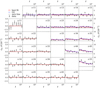 |
Fig. 4. Band power measurements and their best fitting model (see Table A.2). The red curves show the best fitting model fitted to the E-modes (top triangle, |

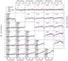 |
Fig. 5. Measurements of the shear correlation functions. The best fitting curves are shown in red (see Table A.2, |

In all three figures we see that the intrinsic alignments of galaxies have the largest effect on the combinations of high- and low-redshift bins, most prominently z-15. The intrinsic alignment signal is dominated by the gravitational-intrinsic (GI) correlations, especially for pairs of tomographic bins where overlap in redshift is minimal, which produces anti-correlations for positive values of AIA. The intrinsic-intrinsic correlations (II) are mostly sub-dominant. The best-fitting value for AIA is in all cases positive (see Table A.2), resulting in a combined signal that is lower than the pure gravitational lensing term.
In Fig. 4 we show the theoretical prediction for the band power B-modes, although these data points are not used in the analysis. The E/B-mode mixing in the band powers is small; nevertheless, it becomes visible at low angular frequencies in the higher-redshift bin combinations, where the E-mode signal is more significant (see Eq. (12)). We find that the B-modes are consistent with zero (p-value = 0.4).
We used the first five COSEBI E-modes for our cosmological analysis and therefore only display them in Fig. 3 (adding more modes has a negligible impact on the constraints, for example see Asgari et al. 2020). G20, however, used both the first 5 and 20 COSEBIs B-modes to test the level of residual systematics in the data, which they found to be consistent with zero in both cases (p-value = 0.04 and 0.38, respectively). As adjacent COSEBI modes are highly correlated (see for example Fig. B.1), we caution the reader against a visual inspection of the goodness-of-fit of the model to the data.
In Table 3 we report the goodness-of-fit of our best-fitting models (corresponding to the maximum of the full posterior), along with point estimates for the best-fitting values of S8. We estimate the degrees of freedom for our data using the effective number of model parameters, NΘ = 4.5 (see Sect. 6.3 of J20). This value was obtained for a mock cosmic shear analysis very similar to ours by fitting a χ2 distribution to a histogram of minimum χ2 values from best fits to 500 mock data vectors. The number of varied parameters (12 for COSEBIs and band powers, 13 for 2PCFs, see Table 2) is substantially larger than NΘ, which can have a significant effect on the goodness-of-fit estimates of the model, especially when the data vector is small. Despite the differences between these two-point statistics, we expect them to have a similar sensitivity to cosmological parameters and therefore employ the same NΘ for all of them. We find acceptable goodness-of-fit for all three summary statistics with p-values (probability to exceed the given χ2) ranging from 0.16 (COSEBIs) to 0.01 (band powers).
Goodness of fit and S8 constraints.
In the last column of Table 3 we show the peak of the marginal distribution of S8 and its credible region derived from the highest posterior density of the marginal distribution. As shown in J20, Sect. 6.4, this estimate can be shifted with regards to the true value of the cosmological parameters. It was therefore proposed to additionally report the maximum a posteriori (MAP) estimate and an associated credible interval using the projected joint highest posterior density, PJ-HPD. With this interval we ensure that the MAP value is within the credible region and in the case of a one-dimensional posterior PJ-HPD reduces to the marginal credible region. We show the MAP and PJ-HPD in the fifth column of Table 3. The best fit values for all parameters are shown in Table A.2. The maximum marginal values are almost identical to the MAP in the case of S8, but can in principle differ more substantially for other parameters. The p-values for band powers and 2PCFs are considerably lower than for COSEBIs; however, since their best-fitting values are very similar, we conclude that this is a result of the noise realisation or low-level systematics that affect 2PCFs and band powers, but do not mimic a cosmological signal.
Cosmic shear results are usually shown in terms of σ8 and Ωm, or S8 and Ωm. In Fig. 6 we show our results for these parameters and compare them to the Planck results. In the left panel we see that the constraints from these three statistics move along the degeneracy direction of σ8 and Ωm; however, they show good agreement in the value of S8 as we saw in Table 3. This movement is expected and will depend on the noise realisation in conjunction with the weighting of the data. In Fig. 1 we saw that our three sets of statistics show varying sensitivities to different angular scales. Hence, we can obtain different parameter constraints given the same noise realisation. We discuss this further and show mock data results in Appendix B.1. The left panel of Fig. 6 shows that the extent of the ξ± contours appears smaller than that of the other statistics. This is because the posterior is truncated at low Ωm by the prior. We also see in Table 3 that the constraints from ξ± for S8 are tighter than those for both COSEBIs and band powers, whereas we would have expected similar constraining power for these three statistics. The right-hand panel of Fig. 6 illustrates that the ξ± contours are horizontal in Ωm and S8, while the marginal posterior for COSEBIs and especially for band powers is tilted, showing that S8 is not perpendicular to the degeneracy between σ8 and Ωm for the latter two statistics.
 |
Fig. 6. Marginalised constraints for the joint distributions of σ8 and Ωm (left), as well as S8 and Ωm (right). The 68% and 95% credible regions are shown for COSEBIs (orange), band powers (pink) and the 2PCFs (cyan). Planck (2018, TT, TE, EE+lowE) results are shown in red. |
The current established definition for S8 is σ8(Ωm/0.3)α, with α = 0.5. Previously (see for example Kilbinger et al. 2013), the value of α was fitted to the contours, to find the tightest constraints from the data. As Fig. 6 clearly shows, α = 0.5 does not provide an optimal description for the σ8-Ωm degeneracy of either COSEBIs or band powers. In general, the value of α depends on the weighting of the angular scales entering the analysis, which probe different physical scales for different redshifts. In order to avoid confusion, we keep the established definition of S8 with α = 0.5, but also include results for
 (14)
(14)
where α is fitted to the contours. In Appendix A we describe our fitting method and show contours for Σ8 and Ωm (see Fig. A.2).
In Table 4 we present best-fitting values for α and constraints for its corresponding Σ8. As expected, α ≈ 0.5 for the 2PCFs, which means that S8 remains a good summary parameter for this composition of the data vector. For COSEBIs and band powers we find α = 0.54 and α = 0.58, respectively, showing that they have a significantly different degeneracy to what is captured with S817. Here we see that the sizes of the Σ8 credible intervals for the different statistics are much closer to each other compared to the S8 constraints in Table 3. The constraints from ξ± are still slightly tighter. We expect this to occur when the noise realisation pushes the contours closer to the edges of the prior region, especially since the halo model used for predicting the matter power spectrum is not calibrated for very high and low values of σ8 and Ωm and therefore becomes less likely to match the data. The standard deviation of the best-fitting Σ8 for COSEBIs is 0.019, for band powers it is 0.020 and for 2PCFs it is 0.018. We note that their central values cannot be directly compared, unless Ωm is fixed to 0.3.
Best-fit Σ8 and Ωm − σ8 degeneracy line.
With our cosmic shear data we can put a tight constraint on the Σ8 parameter, but with the exception of the intrinsic alignment amplitude, AIA, we are largely prior-dominated for the remainder of the sampled parameters (see Table 2). This is also reflected in the effective number of parameters that we record in Table 3. Nevertheless, we show results for other parameter combinations in Appendix A.
4.2. Impact of nuisance parameters and data divisions
In our analysis we have a number of astrophysical and nuisance parameters which are marginalised over. Here we test the sensitivity of our data to the choice of these parameters and their priors. Furthermore, we investigate the impact of removing individual redshift bins from the analysis, as well as the lowest two redshift bins jointly. In the following we first introduce Figs. 7 and 8 and then provide the details of each case.
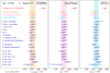 |
Fig. 7. Impact of nuisance parameter treatment and tomographic bin exclusion on Σ8 constraints. Results are shown for COSEBIs (left), band powers (centre) and 2PCFs (right), with fiducial constraints in orange, pink, and cyan, respectively. We use the best-fitting value of α for the fiducial chain of each set of statistics to define Σ8 (Eq. (14)) using the covariance matrix generated from the Tröster et al. (2020a) values instead of the iterative covariance used in Sect. 4.1. The value of α for each panel is given underneath. Two sets of credible regions are shown for each case: the multivariate maximum posterior (MAP, circle) with PJ-HPD (solid) credible interval and the maximum of the Σ8 marginal posterior (diamond) with its highest density credible interval (dot-dashed). The shaded regions follow the fiducial PJ-HPD results of the corresponding statistics. We show Planck results (red), as well as the fiducial results of the other two statistics for the given α of each panel for comparison. Cases 5–12 show the impact of different observational systematics, while cases 13 and 14 show results for the impact of astrophysical systematics. The last six cases present the effect of removing redshift bins and their cross-correlations from the analysis. |
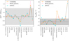 |
Fig. 8. Relative impact of nuisance parameters and the removal of redshift bins. Each of the cases explored in Fig. 7 is compared to their corresponding fiducial results. COSEBIs are shown as orange circles, band powers as pink crosses and 2PCFs as cyan squares. Left: the difference between the upper edge of the marginal Σ8 posterior for each case and its fiducial chain, normalised by half of the length of the marginal credible interval of the case. The grey shaded area indicates the region in which systematic shifts remain below the 1σ statistical error. Right: comparison of constraining power between the fiducial and the other cases. Here α is fitted to each chain separately to find the tightest Σ8 = σ8(Ωm/0.3)α constraint for each case. We show the fractional difference between the standard deviations of the case and the fiducial one. |
The results of these tests are summarised in Fig. 7. Here we use Σ8 with α fitted to the fiducial chain for each of the statistics to assess the impact of the nuisance parameters and the exclusion of redshift bins. We show two sets of point estimates and associated error bars for each case, the MAP and PJ-HPD credible interval, as well as the marginal mode and highest-posterior density credible interval. We note that PJ-HPD intervals are expected to have an error of about 10% in their boundaries (see Sect. 6.4 of J20).
Each panel shows results for one of the two-point statistics, COSEBIs, band powers and 2PCFs; however, in the first section of each panel we also show the fiducial results for the other two cosmic shear statistics (using the same α) and Planck for comparison. The shaded regions correspond to the PJ-HPD credible interval of the fiducial chain for the relevant statistics of each panel. The second section of the figure shows results for the impact of observational systematics. In the third section we explore the effect of astrophysical systematics. The fourth section allows for an inspection of the significance of the data in each redshift bin.
We also test the impact of removing the largest two θ-bins from the analysis of ξ+ and find its impact to be negligible. The mean of S8 is lowered by 0.1σ compared to our fiducial case and its standard deviation is increased by 4%. This final test assesses the Gaussian likelihood approximation since the distribution of ξ+ is significantly non-Gaussian for these bins (see Fig. 17 of J20).
To quantify the impact of the different setups shown in Fig. 7, we extract two key properties of each test analysis, relative to the fiducial case. In the left-hand panel of Fig. 8 we plot the difference between the upper edge of the marginal credible interval shown in Fig. 7 for the fiducial setup,  , and the cases named on the abscissa,
  . We normalise
 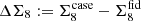 by half of the length of the marginal credible interval that we found for each case, σcase. We chose the upper edge since we are primarily interested in a comparison with the Planck inferred value for Σ8 which is larger than our measurements. We show results for all three statistics, COSEBIs (orange), band powers (pink) and 2PCFs (cyan).
The right-hand panel of Fig. 8 compares the size of the constraints on Σ8 between different cases and the fiducial case. The Σ8 for each case is defined with its own corresponding best-fit α. As the width of the Ωm − σ8 degeneracy is the main parameter that we constrain, this definition allows us to do an approximate figure-of-merit comparison between the different test cases and identify the ones that have a larger impact on our constraining power. For this plot we use the standard deviation of the marginal distributions as they are not affected by smoothing which affects the marginal credible intervals, or by the small number of samples that produce the PJ-HPD. J20 argued for a 0.1σ error on our constraints, coming from smoothing and sampling of the likelihood surfaces to set their requirements on the modelling and data systematics. Here we show the 0.1σ region in grey.
4.2.1. Shear calibration uncertainty
The first nuisance parameter that we consider is the error on the multiplicative shear calibration, m, that is applied to the ellipticity measurements, σm. The value of m is estimated using image simulations (see Sect. 3 and Kannawadi et al. 2019). The assumptions made when producing the image simulations can affect the value of this calibration parameter. In our fiducial chains we absorb this uncertainty into the covariance matrix; however, we could instead allow m to vary as a free model parameter, one per redshift bin. In the covariance matrix estimation we use different values of σm for each redshift bin (see Table 1) and assume that they are fully correlated. To produce the priors for the m parameters, we can take the same approach or instead assume that we do not know the extent of this correlation and use larger uncorrelated priors that encompass any expected correlations between the redshift bins (see for example Hoyle et al. 2018). To do so, we multiply each of the σm values by the square root of the total number of redshift bins,  . This way we produce two setups with free m, labelled “free m correlated” and “free m uncorrelated”.
These setups cover all possible scenarios for the error on m. The m calibration in the simulations is determined per tomographic bin, so that the estimates are independent. However, the surface brightness profiles are modelled as Sersic profiles, and any model bias arising from mismatches with the true morphologies will be shared across the bins. Hence assuming that the m-values are fully correlated, as we have done in the fiducial analysis is an extreme scenario, whereas the scenario where m is uncorrelated represents the other extreme. A more consistent estimate requires multi-band image simulations to capture the correlation between photometric redshift determination and shear estimation.
For the cosmic shear analysis of KV450 a more conservative route was taken, where a σm = 0.02 was employed for all bins, equal to the largest value of σm that we use. Similar to our fiducial analysis, these studies included σm in the covariance matrix, assuming full correlation. Here we also test the effect of this assumption, but with free, correlated m parameters (“free m 0.02”). We then compare all of these setups with a zero σm case (“no σm”) to fully capture the impact of this nuisance parameter18.
Comparing the Σ8 values for these different choices, we see an at most 0.5σ shift corresponding to the “free m correlated” results of the 2PCFs. With the “no σm” and “free m 0.02” cases we do not see a significant change in Σ8. The impact of the uncertainty on m on the standard deviations of the marginal distributions of Σ8 is at most 10%.
4.2.2. Photometric redshift uncertainty
Another component of the data that is calibrated using simulations is the mean of the SOM redshift distribution of galaxies in each tomographic bin. In the fiducial chains we allow for a free δz parameter per redshift bin, but with correlated informative priors, through the covariance matrix between the δz values estimated from the MICE2 simulations (see H20b). To assess the impact of this freedom in the analysis, we fix the δz to their fiducial values (“no σz”). Another case that we consider is the impact of inflating the priors taken from MICE2 by a factor of 3 instead of a factor of 2 that we used in the fiducial case (“inflated σz”). H20b investigated cross-correlations with spectroscopic reference samples as a complementary, independent method for calibrating the redshift distributions. We use their quoted  shifts (see Table 3 of their paper) in combination with their estimated covariance to create the “Clustering-z shifts” case. The δz uncertainty and mean values that we consider here have a negligible impact on our analysis. This is true for both the impact on the marginal value of Σ8 and its constraints, as can be seen in Fig. 8.
4.2.3. Impact of all observational systematics
To evaluate the joint impact of observational systematics, we re-analyse the data by setting m and δz errors to zero. For the 2PCFs chains, we additionally fix the value of δc. We call this setup “no observational systematics”. From Fig. 8 we deduce that the impact of our observational systematics is small, whether we consider them separately or jointly. We remind the reader that variations of order 0.1σ are expected to occur between different instances of the sampling of the same posterior surface.
4.2.4. Sensitivity to astrophysical modelling choices
Our astrophysical nuisance parameters are the baryon feedback parameter, Abary, and the amplitude of the intrinsic alignments of galaxies, AIA. We test the impact of Abary by assuming a no-feedback case with Abary fixed to 3.13 (“no baryons”). As illustrated by Fig. 8 the no-baryons case has a significantly larger effect on ξ±, which is expected since the 2PCFs are more sensitive to small physical scales as we saw in Fig. 1. Contrary to expectations, COSEBIs appear to be more sensitive to baryon feedback compared to the band powers. This is not caused by the scale sensitivity, but is rather a result of this particular noise realisation. In Fig. A.3 we can see that the constraints on Abary for band powers are skewed towards larger values, indicating that they prefer a model with weaker baryon feedback (see also Table A.2). Therefore, the difference between band powers analysed with and without baryon feedback is smaller than for COSEBIs, which have a rather uniform Abary marginal distribution. For the 2PCFs, however, we find a similarly uniform distribution. The increased sensitivity of the 2PCFs to baryon feedback is thus a result of the small scales that impact their modelling. This is true for both the upper edge of the marginal credible region and to a lesser extent the width of the constraints for Σ8. In Appendix B.1 we discuss that the marginal distributions of poorly constrained parameters, such as Abary, can be skewed due to noise in the data.
In our fiducial analysis we assume that the amplitude of the intrinsic alignment model, which describes the response of projected galaxy ellipticities to the local quadrupole of the dark matter distribution, is independent of redshift (see Sect. 2.4 of J20). However, this model can be modified empirically to include a redshift dependence (see Eq. (16) of J20), by multiplying its three-dimensional power spectra with factors of
 (15)
(15)
As a test case we allow ηIA to vary uniformly in [ − 5, 5] and set zpivot = 0.3 for a more straightforward comparison with previous KiDS and intrinsic alignment analyses (for instance Joachimi et al. 2011). We call this case “redshift-dependent IA”.
In Fig. 8 we see that the redshift dependence of AIA has little impact on the upper edge of the marginal credible region of Σ8, however it can result in wider constraints. This redshift-dependence for the COSEBIs analysis produces a bimodal likelihood distribution, which results in a larger standard deviation. This is not seen with the other two statistics, which we therefore conclude is an effect of the cross-talk between the noise realisation and this extra freedom in the analysis. This has been seen in other analyses, when the additional redshift of the intrinsic alignment model is allowed to vary within broad priors (for example Joudaki et al. 2017a, 2020; Asgari et al. 2020). The inclusion of this freedom in the analysis does not impact the goodness-of-fit in a significant way.
4.2.5. Removing tomographic redshift bins
Aside from the effect of nuisance parameters, we determine the impact of each tomographic redshift bin by removing them and their cross-correlations in turn from the data vector. These results are labelled as “no z-bin i”, with i denoting the removed redshift bin. The first two redshift bins have a lower signal-to-noise and are mostly sensitive to the intrinsic alignments of galaxies. To capture the impact of an unconstrained intrinsic alignment model, we also run chains where both redshift bins 1 and 2 are removed from the analysis (“no z-bins 1 and 2”).
Of these setups the no z-bin 4 case has the largest impact on Σ8 marginal values (left panel of Fig. 8). For this case, depending on the statistics used, we obtain between 1.1σcase to 1.8σcase differences in Σ8. The significance of these shifts however depends on which values from the distributions are compared with each other. For example, for the no z-bin 5 case we find larger deviations if we consider the maximum of the marginal distribution or the MAP values. In Appendix B.2 we perform a series of internal consistency tests which do not flag the differences between these redshift bins as statistically significant.
When removing redshift bins we see that the constraining power does not change by more than 0.15σ unless the fifth bin is removed (right panel of Fig. 8). Without this bin our errorbars inflate by 60%. This shows that the inclusion of higher-redshift bins is crucial for increasing the statistical power of a cosmic shear analysis.
4.3. Internal consistency
In this section we summarise our internal consistency results. For details see Appendix B.1 and Appendix B.2.
Our cosmological analysis has been performed independently, using three sets of two-point statistics. We do not expect to find the exact same constraints from these statistics, since they place different weights on a given angular scale. That said, the statistics are measured within the same survey volume and using the same galaxies, so that it is reasonable to assume some level of redundancy between these measurements. Given these two competing factors, it is not immediately clear what level of variation is expected. In other words, are the results in Table 3 consistent? Or is the difference between S8 constraints caused by systematic effects being picked up by one statistic but not another?
To answer these questions, we apply a series of tests on mock data realisations, produced from multivariate Gaussian distributions. In our primary test we draw correlated noise realisations given the full covariance, including cross-correlations between 2PCFs, COSEBIs and band powers, estimated from the SALMO simulations (see Fig. B.1). We choose a fiducial cosmology and create 100 realisations of the data vector, including all three sets of two-point statistics. We analyse each set and realisation separately with a similar setup to our fiducial analysis explained in Sect. 3 and derive parameter constraints. We compare the maximum of the marginal distributions for S8 between the two-point statistics for each realisation and find that the distribution of  , where
  are the maximum marginal values for one of the statistics, is only 20 − 30% narrower than the width of the marginal distributions for S8 per two-point statistic. Therefore, we conclude that differences of up to 0.7 − 0.8σ between the results of COSEBIs, 2PCFs and band powers are expected to occur frequently (for about 68% of the realisations). For our KiDS-1000 analysis we find the maximum ΔS8 for the marginal posterior modes of COSEBIs and 2PCFs, which is a difference of about 0.4σ.
Among the significantly constrained parameters in our data analysis, only AIA displays a notable difference, with the marginal posterior peaking roughly at double the value for band powers in comparison with correlation functions and COSEBIs. In our mock analysis we see differences of this level or higher in AIA in 5% of the cases. Given the full consistency between the S8 values we conclude that the results between the three sets of summary statistics are in agreement.
While the two-point statistics have different scale sensitivities, we expect their response to biases in the redshift distributions to be similar, as that will mainly affect the relative amplitude of the data vectors. H20b conducted tests of the KiDS-1000 redshift distributions by comparing them with simulations as well as cross-correlations with clustering-redshifts as discussed in Sects. 3 and 4.2. However, we note that these tests are not very sensitive to discrepancies that may exist in the tails of the redshift distributions, beyond their impact on the mean redshift.
We also follow the methodology of Köhlinger et al. (2019) and perform three tiers of Bayesian consistency tests, comparing the cosmological inference from all bin combinations involving a given redshift bin with that from the remainder of the data vector. We find consistent results between all redshift bins, except for the second tomographic bin which covers the range 0.3 < zB < 0.5. Analyses using this bin and its cross-correlations, compared to using all other bins, produce results that conflict by up to 3σ in some parameters (for more details see Appendix B.2). Also in Fig. A.4 we see that the data favours a δz, 2 parameter that shift the redshift distribution of this bin to larger values. While this inconsistency warrants further investigation in the future, we find that removing the second redshift bin, or indeed the first and second bin, from the analysis has a negligible impact on the cosmological parameter constraints (see Sect. 4.2.5).
4.4. Comparison with other surveys
In this section we compare our parameter constraints with previous results from cosmic shear surveys and Planck. Figure 9 contrasts our S8 constraints with a selection of recent cosmic shear results shown in green (see Fig. A.5 for an extended selection). The final entry shows the Planck results. For each case we show two sets of error bars, corresponding to the marginal highest-posterior density region and the PJ-HPD. Since we do not have a good estimate of the MAP from the public chains, we do not show best-fitting values for the external cosmic shear results.
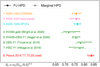 |
Fig. 9. Comparison between S8 values for different surveys. All results are shown for both multivariate maximum posterior (MAP) and PJ-HPD (upper solid bar), as well as the marginal mode and the marginal S8 credible interval (lower dot-dashed bar). The top three points show our fiducial KiDS-1000 results. The next four show a selection of recent cosmic shear analyses from external data as well as previous KiDS data releases. We note that S8 does not fully capture the degeneracy direction for all of the analysis above (see the discussion in Sect. 4.1 and Appendix A). For example for the HSC-Y1 contours α = 0.45 was found to be the best fitting power. The last entry shows the Planck 2018 (TT, TE, EE+lowE) constraints. An extended version of this plot can be found in Appendix A. |
The different cosmic shear analysis presented in Fig. 9 constrain slightly different degeneracy directions in the σ8 − Ωm plane and therefore S8 does not necessarily capture their best constrained parameter combination. Hence we also compare the results of these surveys in the S8 − Ωm plane displayed in Fig. 10. We note that for all cosmic shear analyses presented here, the Ωm constraints are prior dominated. Consequently, no meaningful conclusions can be drawn from the differences that can be seen in the figure when it comes to this parameter.
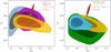 |
Fig. 10. Comparison between KiDS-1000 and other surveys in the S8 − Ωm plane. The fiducial KiDS-1000 results which use COSEBIs (orange) and the Planck primary anisotropy constraints (red) are shown in both panels. The DES-Y1 results of Troxel et al. (2018b, purple) and HSC-Y1 results of Hikage et al. (2019, grey) are shown in the left panel, while the KV450 constraints of Wright et al. (2020a, green) and the joint KV450 and DES-Y1 results of Asgari et al. (2020, blue) are shown in the right panel. A summary of these constraints in S8 can be found in Fig. 9. |
Of the external cosmic shear data, the Wright et al. (2020a) result is the closest to our methodology in terms of the calibration of the redshift distributions. This KV450 analysis employed 2PCFs measured on less than half of the imaging area that we analyse (777 deg2 versus 341 deg2). We find that our results are in good agreement with Wright et al. (2020a), with the multivariate maximum posterior values of S8 agreeing to within 0.003 for the 2PCFs, the statistics used in both19. Marginal errors decrease by more than a factor two, reflecting the increase in survey area, and the reduced impact of calibration uncertainties in our KiDS-1000 analysis. Our KiDS-1000 constraints are similar to the joint KV450 and DES-Y1 analysis of Asgari et al. (2020) both in their constraining power and value. We find that the DES-Y1 and HSC-Y1 results of Troxel et al. (2018b) and Hikage et al. (2019) are also both in agreement with our constraints. It is evident from this plot that all of these cosmic shear analyses measure a lower S8 than the Planck inferred value under a flat ΛCDM model, although with varying levels of significance.
We use two complementary methods to estimate the level of tension between our results and Planck. For this we choose the COSEBIs analysis, which has the best goodness of fit. The first method is to simply compare the results in Σ8, the only parameter that we can set tight constraints on with cosmic shear that is also shared by Planck. We use the conventional method,
![Mathematical equation: $$ \begin{aligned} \tau = \frac{\overline{\phi }^{Planck}-\overline{\phi }^\mathrm{COSEBIs}}{\sqrt{\mathrm{Var}[\phi ^{Planck}]+\mathrm{Var}[\phi ^\mathrm{COSEBIs}]}}\; \end{aligned} $$](/articles/aa/full_html/2021/01/aa39070-20/aa39070-20-eq51.gif) (16)
(16)
where ϕ is either S8 or Σ8,  is the mean of ϕ and Var[ϕ] is its variance. With this definition we find that the Planck predictions are 3.4σ larger than our measured Σ8 value. The difference in S8 is 3σ, but note that this parameter does not fully capture the tension due to the residual correlation with Ωm. We use a complementary method which takes the full shape of the marginal distributions into account, bypassing the Gaussian distribution assumption used in Eq. (16), and find slightly larger values of 3.2σ for S8 and 3.5σ for Σ8 (Hellinger; see Appendix F.1 of Heymans et al. 2020 for details). These methods of estimating differences between cosmological analyses ignore the possible complexities of the multi-dimensional parameter space. Other methods that test consistencies within the full posterior are generally less stable owing to the difficulty in estimating the statistical properties of this distribution to a sufficiently high accuracy. On the other if the tension is truly in one aspect of the model, summarised in a single parameter, then including extra dimensions to the tension metric will likely dilute the significance of the results.
A Bayesian approach compares the full likelihood between an analysis of the two sets of data separately and their combined analysis. The Bayes factor can be used in conjunction with the Jeffreys’ scale to assess the tension between the data sets. We find that the base 10 logarithm of the Bayes factor is 0.54 − 1.15, with a preference for two separate cosmologies, corresponding to a substantial to strong evidence for disagreement (the two values are estimated via the importance nested sampling and the traditional methods, see Appendix B.2 for more details). This result is in qualitative agreement with the simple marginal distribution comparison above. Handley & Lemos (2019) suggested using a different measure called suspiciousness, S, which is less sensitive to the choice of priors compared to the raw evidence comparison of the Bayes factor. We measure this quantity but are unable to cast it into a meaningful scale of disagreement. To do so we need to have a robust measure of the degrees of freedom for Planck, KiDS-1000 and their joint analysis. In J20 we saw that the dimensionality method that is currently used in conjunction with suspiciousness produces biased estimates of the effective number of parameters (see Appendix B.3 for more details). The alternative methods proposed there require analysing many mock realisations of the data with computationally expensive posterior sampling. Future work is required to develop a robust way to derive the sampling distribution for suspiciousness.
5. Summary and conclusions
We have presented a cosmic shear analysis of the fourth Data Release of the Kilo-Degree Survey (KiDS-1000, Kuijken et al. 2019), making use of circa 1000 deg2 of deep nine-band optical-to-infrared photometry with exquisite image quality in the r-band for gravitational shear estimates. In addition to more than doubling the survey area with respect to earlier KiDS analyses (Hildebrandt et al. 2020a), this work incorporated the following major updates:
-
The galaxies entering our five tomographic redshift bins are selected to have good representation by objects with spectroscopic redshifts (the “gold” sample), which are subsequently re-weighted via an unsupervised machine learning approach to provide accurate redshift distributions (Wright et al. 2020b; Hildebrandt et al. 2020b).
-
The multiplicative shear calibration is based on image simulations containing COSMOS-emulated galaxies (Kannawadi et al. 2019). This analysis was repeated for the new sample selection, with a revised determination of the residual calibration uncertainties that is now derived per tomographic bin from the spread in a number of conservative settings implemented in the simulations.
-
The accuracy of the covariance models, likelihood, and inference pipeline has been validated on an extensive suite of KiDS-1000 mock catalogues. The key cosmological quantity constrained by cosmic shear, the parameter S8 = σ8(Ωm/0.3)0.5, is now used as a sampling parameter in evaluating the posterior, enabling us to impose a wide top-hat prior that is more conservative than previous analyses relying on the primordial power spectrum amplitude, As, or a function thereof.
-
The analysis was conducted independently with three cosmic shear two-point statistics: the angular shear correlation functions ξ±, Complete Orthogonal Sets of E/B-Integrals (COSEBIs), and angular band powers. The latter two are constructed as linear combinations of ξ± that offer a clean separation into cosmological E-modes and systematics-driven B-modes (exact for COSEBIs and approximate for band powers), as well as additional data compression (the COSEBIs and band powers data vectors are 66% and 46% smaller than the 2PCFs data vector). Both derived statistics inherit the beneficial lack of sensitivity to the survey mask and galaxy ellipticity noise from the correlation functions, but avoid the very broad responses of ξ± to Fourier modes, which lead to increased non-Gaussianity in the likelihood due to small ℓ-modes and increased sensitivity to small-scale features in the modelling (large ℓ-modes), such as baryon feedback.
These additions have increased the constraining power of KiDS with little change in our best-fitting value for S8. Comparing the similar setups of our correlation function analysis with the results from Wright et al. (2020a) who worked with KiDS Data Release 3, we find a decrease in the marginal S8 errors by 54%. The marginal posterior mode of S8 has increased by 0.05 in KiDS-1000; however, the multivariate maximum posterior agrees to within 3 × 10⁻³ for the two analyses, so the shift in the marginal distribution is solely due to the different shape of the posterior distribution. Our results are in good agreement with those of the DES and HSC surveys, reducing marginal S8 errors by 14% with respect to Troxel et al. (2018b) and by 32% with respect to Hikage et al. (2019).
From a theoretical point of view we conclude that there is a strong case for favouring COSEBIs and/or band power statistics over the standard shear correlation functions in the likelihood analysis, with COSEBIs providing the cleanest and most compact data vector, and band powers offering intuition through directly tracing the angular power spectra predicted from theory. Both of these methods allow for an E and B-mode decomposition, which are mixed with each other in the case of the correlation functions. This will be of particular importance for analysis of future data with improved constraining power.
Despite these differences, we find the KiDS-1000 S8 constraints derived from the three statistics to be in excellent agreement. Due to the different scales probed, the analyses trace different sections of the Ωm − σ8 degeneracy line, which causes S8 to not fully capture the constraining power transverse to the degeneracy in all cases. Fitting the parameter Σ8 = σ8(Ωm/0.3)α to the posterior, we find a best fit of α = 0.51 for ξ±, which means that S8 is very close to the optimal summary parameter as found in previous KiDS analyses. For COSEBIs and band powers, α = 0.54 and 0.58, respectively. The constraining power on the optimal Σ8 is then nearly identical between the three statistics.
Constraining a spatially flat ΛCDM model, we obtain  for our fiducial setup using COSEBIs. The quoted values are extracted from the mode and highest posterior density of the marginal S8 posterior (denoted by M-HPD). Since the analysis of mock data shows that the marginal posterior mode or mean can be shifted significantly from the global best fit, due to a high-dimensional posterior with complex shape, we additionally provide the multivariate posterior maximum with an associated projected credible interval (PJ-HPD),
  . For KiDS-1000 cosmic shear the two credible intervals are in very good agreement though, with nearly identical point estimates for S8 and credible interval sizes differing by less than 5% (this is also true for Planck CMB constraints). The goodness of fit is acceptable, ranging from a p-value of 0.16 for COSEBIs to 0.03 for 2PCFs and 0.01 for band powers. Since the latter two preferentially extract information from higher angular frequencies relative to COSEBIs, this could indicate an as yet insignificant limitation in our non-linear modelling, for example in the intrinsic alignment of galaxies. On the other hand given the consistency between the values of S8 for COSEBIs, 2PCFs, and band powers, this could be a result of an unfortunate noise realisation that affects the higher ℓ-modes.
Due to the tighter constraints of KiDS-1000, the tension in Σ8 with Planck Collaboration VI (2020) has increased to 3.4σ, meaning that there is a 7 in 10 000 chance of a mere statistical fluctuation between the low and high-redshift probes assuming Gaussian distributions (3σ in the less constrained S8). Whether this discrepancy is mitigated by extensions to our cosmological model will be further investigated by Tröster et al. (in prep.), but the most obvious routes are unlikely to provide a satisfactory solution. For instance, KiDS and Planck would be reconciled in significantly open cosmologies (Joudaki et al. 2017a), but Planck prefers a positive curvature whose significance is still under debate (see Efstathiou & Gratton 2020 and references therein). We argue that the tension with the CMB indeed manifests in the parameter S8 (or Σ8 if S8 retains significant correlations with Ωm), as was also observed in Tröster et al. (2020a). Bayesian tension measures that act on the full shared parameter space between KiDS and Planck are also provided, showing a substantial to strong evidence for disagreement.
We demonstrate that our constraints are robust to changes in the calibration procedures of multiplicative calibration in gravitational shear estimates, as well as of the redshift distributions. The S8 credible intervals are not significantly affected by these changes either, which indicates that the KiDS-1000 constraints are statistics dominated. We also find no unexpected shifts in the inferred S8 value when removing baryon feedback from the matter power spectrum model, when introducing additional flexibility to the intrinsic alignment model, or when removing all tomographic bin combinations involving a certain bin from the data vector. A Bayesian internal consistency analysis of tomographic bin splits reveals significant tension (up to 3σ) when isolating all bin combinations involving the second bin, whose signals have higher amplitude than expected for its mean redshift. This will be a priority to investigate further in forthcoming work. However, excluding all elements of the KiDS-1000 data vector dependent on the second bin does not affect our cosmological constraints, which we therefore consider robust to this effect.
Looking ahead to the Legacy analysis of the complete KiDS survey, the statistical power of cosmic shear measurements is going to further improve thanks to a 35% increase in sky area and a second pass in the i-band over the full survey. New, dedicated VST observations in spectroscopic survey fields will consolidate the redshift calibration and yield gains especially at redshifts beyond unity, unlocking the potential for very high signal-to-noise cosmic shear signals beyond our current highest-redshift bin. An upgrade to full multi-band image simulations will improve both the precision and accuracy of the shear calibration. Together with the innovation and cross-comparison opportunities provided by the contemporaneous DES and HSC cosmic shear measurements, we can therefore be optimistic that decisive new insights into the structure-growth tension will be delivered even before the next generation of powerful weak lensing surveys will begin to take data.
Legacy Survey of Space and Time; https://www.lsst.org
Formerly Wide Field Infrared Survey Telescope; https://nasa.gov/wfirst
We note that the Hamana et al. (2020) re-analysis of HSC with 2PCFs, find an S8 value that is closer to Planck, albeit still lower by ∼1σ.
Effects such as contributions beyond the Born approximation (Schneider et al. 1998), source clustering (Schneider et al. 2002b), intrinsic alignment models with tidal effects (for instance Blazek et al. 2015) and certain alternative cosmological models (see for example Thomas et al. 2017) are able to produce B-modes. For current surveys, however, these effects are negligible.
From here on we drop the redshift dependence of Cϵϵ(ℓ) as that has no effect on the linear transformations that produce our two-point statistics.
Speedy Acquisition of Lensing and Matter Observables.
KCAP will become public once the KiDS-1000 analysis papers are accepted. Early access can be granted to interested parties on request.
Data products are made freely accessible through: http://kids.strw.leidenuniv.nl/DR4
We run the Nelder-Mead minimiser with the adaptive option, which is more reliable for higher dimensional and multi-modal problems. See docs.scipy.org/doc/scipy/reference/optimize.minimize-neldermead.html.
G20 show that the 2D c-term is negligible. Therefore, we omit this term in our modelling.
Except for the integrated Sachs–Wolfe effect which has a low-level impact on the CMB constraints.
We note that in all cases the data is reported at discrete points, as a result of binning for 2PCFs and band powers, or by definition in the case of COSEBIs. Hence, the theory values are also discrete, although connected to each other for visual guidance.
The fit error for α is about 10−3.
For all the cases where σm is not included in the covariance matrix, the fiducial m correction is applied to the theory rather than the data vectors.
The MAP value for Wright et al. (2020a) is taken from the MULTINEST chain, S8 = 0.765.
The posterior at the origin is estimated from a fit to the sampled posterior, using a kernel density estimation with a Gaussian.
We have seen even more significant differences when including some of the poorly constrained parameters. For example, when comparing the parameter estimates for Δ(S8, AIA, Ωm) we find differences of up to 3.6σ, however as Ωm is not significantly constrained by our data, this more significant value may just be a result of additional fluctuations in the noise.
Acknowledgments
The chains are plotted with CHAINCONSUMER (Hinton 2016): samreay.github.io/ChainConsumer. We are grateful to Eric Tittley, especially for saving our data. We thank Matthias Bartelmann, out external blinder, for keeping the key to our blinded data, which he revealed to us on the 9th of July. We also acknowledge Joe Zuntz for his help over the years with COSMOSIS. We thank Joachim Harnois-Déraps, Shahab Joudaki, Mohammadjavad Vakili and Ziang Yan for useful discussions. We are also thankful to the anonymous referee for their constructive comments. This project has received funding from the European Union’s Horizon 2020 research and innovation programme: We acknowledge support from the European Research Council under Grant agreement No. 647112 (C.H., M.A., C.L., B.G. and T.T.) and 770935 (H.Hi, A.H.W., A.D. and J.LvdB). C.L. is grateful for the working environment kindly provided by WPC Systems Ltd. during the pandemic. TT acknowledges support under the Marie Skłodowska-Curie Grant agreement No. 797794. C.H. acknowledges support from the Max Planck Society and the Alexander von Humboldt Foundation in the framework of the Max Planck-Humboldt Research Award endowed by the Federal Ministry of Education and Research. H. Hi is supported by a Heisenberg grant of the Deutsche Forschungsgemeinschaft (Hi 1495/5-1). H. Ho acknowledges support from Vici Grant 639.043.512, financed by the Netherlands Organisation for Scientific Research (NWO). K.K. acknowledges support by the Alexander von Humboldt Foundation. This work was partially enabled by funding from the UCL Cosmoparticle Initiative (BS). M.B. is supported by the Polish Ministry of Science and Higher Education through Grant DIR/WK/2018/12, and by the Polish National Science Center through grants no. 2018/30/E/ST9/00698 and 2018/31/G/ST9/03388. J.T.A.dJ. is supported by the Netherlands Organisation for Scientific Research (NWO) through grant 621.016.402. L.M. acknowledges support from STFC Grant ST/N000919/1. HYS acknowledges the support from NSFC of China under Grant 11973070, the Shanghai Committee of Science and Technology grant No.19ZR1466600 and Key Research Program of Frontier Sciences, CAS, Grant No. ZDBS-LY-7013. The KiDS-1000 results in this paper are based on data products from observations made with ESO Telescopes at the La Silla Paranal Observatory under programme IDs 177.A-3016, 177.A-3017 and 177.A-3018, and on data products produced by Target/OmegaCEN, INAF-OACN, INAF-OAPD and the KiDS production team, on behalf of the KiDS consortium. Author contributions: All authors contributed to the development and writing of this paper. The authorship list is given in three groups: the lead authors (M.A., C.L., B.J.) followed by two alphabetical groups. The first alphabetical group includes those who are key contributors to both the scientific analysis and the data products. The second group covers those who have either made a significant contribution to the data products, or to the scientific analysis.
References
- Aihara, H., Arimoto, N., Armstrong, R., et al. 2018, PASJ, 70, S4 [NASA ADS] [Google Scholar]
- Alam, S., Ata, M., Bailey, S., et al. 2017, MNRAS, 470, 2617 [NASA ADS] [CrossRef] [Google Scholar]
- Albrecht, A., Bernstein, G., Cahn, R., et al. 2006, ArXiv e-prints [arXiv:astro-ph/0609591] [Google Scholar]
- Alonso, D., Sanchez, J., Slosar, A., & LSST Dark Energy Science Collaboration 2019, MNRAS, 484, 4127 [CrossRef] [Google Scholar]
- Asgari, M., & Schneider, P. 2015, A&A, 578, A50 [NASA ADS] [CrossRef] [EDP Sciences] [Google Scholar]
- Asgari, M., & Heymans, C. 2019, MNRAS, 484, L59 [NASA ADS] [CrossRef] [Google Scholar]
- Asgari, M., Schneider, P., & Simon, P. 2012, A&A, 542, A122 [NASA ADS] [CrossRef] [EDP Sciences] [Google Scholar]
- Asgari, M., Heymans, C., Blake, C., et al. 2017, MNRAS, 464, 1676 [NASA ADS] [CrossRef] [Google Scholar]
- Asgari, M., Taylor, A., Joachimi, B., & Kitching, T. D. 2018, MNRAS, 479, 454 [NASA ADS] [Google Scholar]
- Asgari, M., Heymans, C., Hildebrandt, H., et al. 2019, A&A, 624, A134 [NASA ADS] [CrossRef] [EDP Sciences] [Google Scholar]
- Asgari, M., Tröster, T., Heymans, C., et al. 2020, A&A, 634, A127 [NASA ADS] [CrossRef] [EDP Sciences] [Google Scholar]
- Audren, B., Lesgourgues, J., Benabed, K., & Prunet, S. 2013, JCAP, 2013, 001 [NASA ADS] [CrossRef] [Google Scholar]
- Bacon, D. J., Refregier, A. R., & Ellis, R. S. 2000, MNRAS, 318, 625 [NASA ADS] [CrossRef] [Google Scholar]
- Barreira, A., Krause, E., & Schmidt, F. 2018, JCAP, 10, 053 [NASA ADS] [CrossRef] [Google Scholar]
- Bartelmann, M., & Schneider, P. 2001, Phys. Rep., 340, 291 [NASA ADS] [CrossRef] [Google Scholar]
- Becker, M. R., & Rozo, E. 2016, MNRAS, 457, 304 [NASA ADS] [CrossRef] [Google Scholar]
- Becker, M. R., Troxel, M. A., MacCrann, N., et al. 2016, Phys. Rev. D, 94, 022002 [NASA ADS] [CrossRef] [Google Scholar]
- Begeman, K., Belikov, A. N., Boxhoorn, D. R., & Valentijn, E. A. 2013, Exp. Astron., 35, 1 [NASA ADS] [Google Scholar]
- Benítez, N. 2000, ApJ, 536, 571 [Google Scholar]
- Benítez, N., Ford, H., Bouwens, R., et al. 2004, ApJS, 150, 1 [NASA ADS] [CrossRef] [Google Scholar]
- Blazek, J., Vlah, Z., & Seljak, U. 2015, JCAP, 2015, 015 [NASA ADS] [CrossRef] [Google Scholar]
- Bridle, S., & King, L. 2007, New J. Phys., 9, 444 [NASA ADS] [CrossRef] [Google Scholar]
- Brinckmann, T., & Lesgourgues, J. 2018, ArXiv e-prints [arXiv:1804.07261] [Google Scholar]
- Brown, M. L., Taylor, A. N., Bacon, D. J., et al. 2003, MNRAS, 341, 100 [NASA ADS] [CrossRef] [Google Scholar]
- Carretero, J., Castander, F. J., Gaztañaga, E., Crocce, M., & Fosalba, P. 2015, MNRAS, 447, 646 [NASA ADS] [CrossRef] [Google Scholar]
- Crocce, M., Castander, F. J., Gaztañaga, E., Fosalba, P., & Carretero, J. 2015, MNRAS, 453, 1513 [NASA ADS] [CrossRef] [Google Scholar]
- de Jong, J. T. A., Verdoes Kleijn, G. A., Boxhoorn, D. R., et al. 2015, A&A, 582, A62 [NASA ADS] [CrossRef] [EDP Sciences] [Google Scholar]
- de Jong, J. T. A., Kleijn, G. A. V., Erben, T., et al. 2017, A&A, 604, A134 [NASA ADS] [CrossRef] [EDP Sciences] [Google Scholar]
- Drlica-Wagner, A., Sevilla-Noarbe, I., Rykoff, E. S., et al. 2018, ApJS, 235, 33 [NASA ADS] [CrossRef] [Google Scholar]
- Edge, A., Sutherland, W., Kuijken, K., et al. 2013, Messenger, 154, 32 [Google Scholar]
- Efstathiou, G., & Gratton, S. 2020, MNRAS, 496, L91 [CrossRef] [Google Scholar]
- Erben, T., Hildebrandt, H., Miller, L., et al. 2013, MNRAS, 433, 2545 [NASA ADS] [CrossRef] [Google Scholar]
- Euclid Collaboration (Knabenhans, M., et al.) 2019, MNRAS, 484, 5509 [NASA ADS] [CrossRef] [Google Scholar]
- Fenech Conti, I., Herbonnet, R., Hoekstra, H., et al. 2017, MNRAS, 467, 1627 [NASA ADS] [Google Scholar]
- Feroz, F., Hobson, M. P., Cameron, E., & Pettitt, A. N. 2019, Open J. Astrophys., 2, 10 [Google Scholar]
- Fortuna, M. C., Hoekstra, H., Joachimi, B., et al. 2021, MNRAS, 501, 2983 [CrossRef] [Google Scholar]
- Fosalba, P., Crocce, M., Gaztañaga, E., & Castander, F. J. 2015a, MNRAS, 448, 2987 [NASA ADS] [CrossRef] [Google Scholar]
- Fosalba, P., Gaztañaga, E., Castander, F. J., & Crocce, M. 2015b, MNRAS, 447, 1319 [NASA ADS] [CrossRef] [Google Scholar]
- Giblin, B., Heymans, C., Asgari, M., et al. 2021, A&A, 645, 105 [Google Scholar]
- Górski, K. M., Hivon, E., Banday, A. J., et al. 2005, ApJ, 622, 759 [NASA ADS] [CrossRef] [Google Scholar]
- Hamana, T., Shirasaki, M., Miyazaki, S., et al. 2020, PASJ, 72, 16 [CrossRef] [Google Scholar]
- Handley, W. 2019, J. Open Sour. Softw., 4, 1414 [NASA ADS] [CrossRef] [Google Scholar]
- Handley, W., & Lemos, P. 2019, Phys. Rev. D, 100, 043504 [NASA ADS] [CrossRef] [Google Scholar]
- Handley, W. J., Hobson, M. P., & Lasenby, A. N. 2015, MNRAS, 453, 4384 [NASA ADS] [CrossRef] [Google Scholar]
- Heymans, C., Brown, M. L., Barden, M., et al. 2005, MNRAS, 361, 160 [NASA ADS] [CrossRef] [Google Scholar]
- Heymans, C., Grocutt, E., Heavens, A., et al. 2013, MNRAS, 432, 2433 [NASA ADS] [CrossRef] [Google Scholar]
- Heymans, C., Tröster, T., Asgari, M., et al. 2020, ArXiv e-prints [arXiv:2007.15632] [Google Scholar]
- Hikage, C., Takada, M., Hamana, T., & Spergel, D. 2011, MNRAS, 412, 65 [NASA ADS] [CrossRef] [Google Scholar]
- Hikage, C., Oguri, M., Hamana, T., et al. 2019, PASJ, 71, 43 [NASA ADS] [CrossRef] [Google Scholar]
- Hildebrandt, H., Viola, M., Heymans, C., et al. 2017, MNRAS, 465, 1454 [Google Scholar]
- Hildebrandt, H., Köhlinger, F., van den Busch, J. L., et al. 2020a, A&A, 633, A69 [NASA ADS] [CrossRef] [EDP Sciences] [Google Scholar]
- Hildebrandt, H., van den Busch, J. L., Wright, A. H., et al. 2020b, ArXiv e-prints [arXiv:2007.15635] [Google Scholar]
- Hinton, S. R. 2016, J. Open Sour. Softw., 1, 00045 [NASA ADS] [CrossRef] [Google Scholar]
- Hoekstra, H. 2004, MNRAS, 347, 1337 [NASA ADS] [CrossRef] [Google Scholar]
- Hoekstra, H., Herbonnet, R., Muzzin, A., et al. 2015, MNRAS, 449, 685 [NASA ADS] [CrossRef] [Google Scholar]
- Hoffmann, K., Bel, J., Gaztañaga, E., et al. 2015, MNRAS, 447, 1724 [NASA ADS] [CrossRef] [Google Scholar]
- Howlett, C., Lewis, A., Hall, A., & Challinor, A. 2012, JCAP, 4, 027 [NASA ADS] [CrossRef] [Google Scholar]
- Hoyle, B., Gruen, D., Bernstein, G. M., et al. 2018, MNRAS, 478, 592 [Google Scholar]
- Hu, W. 1999, ApJ, 522, L21 [Google Scholar]
- Huff, E. M., Eifler, T., Hirata, C. M., et al. 2014, MNRAS, 440, 1322 [NASA ADS] [CrossRef] [Google Scholar]
- Jarvis, M. 2015, TreeCorr: Two-point Correlation Functions, Astrophys. Source Code Libr. [record ascl:1508.007] [Google Scholar]
- Jarvis, M., Bernstein, G., & Jain, B. 2004, MNRAS, 352, 338 [Google Scholar]
- Jee, M. J., Tyson, J. A., Hilbert, S., et al. 2016, ApJ, 824, 77 [NASA ADS] [CrossRef] [Google Scholar]
- Joachimi, B., Mandelbaum, R., Abdalla, F. B., & Bridle, S. L. 2011, A&A, 527, A26 [NASA ADS] [CrossRef] [EDP Sciences] [Google Scholar]
- Joachimi, B., Lin, C. A., Asgari, M., et al. 2020, ArXiv e-prints [arXiv:2007.01844] [Google Scholar]
- Joudaki, S., Mead, A., Blake, C., et al. 2017a, MNRAS, 471, 1259 [NASA ADS] [CrossRef] [Google Scholar]
- Joudaki, S., Blake, C., Heymans, C., et al. 2017b, MNRAS, 465, 2033 [NASA ADS] [CrossRef] [Google Scholar]
- Joudaki, S., Hildebrandt, H., Traykova, D., et al. 2020, A&A, 638, L1 [CrossRef] [EDP Sciences] [Google Scholar]
- Kaiser, N. 1992, ApJ, 388, 272 [Google Scholar]
- Kaiser, N., Wilson, G., & Luppino, G. A. 2000, ArXiv e-prints [arXiv:astro-ph/0003338] [Google Scholar]
- Kannawadi, A., Hoekstra, H., Miller, L., et al. 2019, A&A, 624, A92 [NASA ADS] [CrossRef] [EDP Sciences] [Google Scholar]
- Kilbinger, M. 2015, Rep. Prog. Phys., 78, 086901 [Google Scholar]
- Kilbinger, M., Fu, L., Heymans, C., et al. 2013, MNRAS, 430, 2200 [NASA ADS] [CrossRef] [Google Scholar]
- Kilbinger, M., Heymans, C., Asgari, M., et al. 2017, MNRAS, 472, 2126 [Google Scholar]
- Köhlinger, F., Viola, M., Valkenburg, W., et al. 2016, MNRAS, 456, 1508 [NASA ADS] [CrossRef] [Google Scholar]
- Köhlinger, F., Viola, M., Joachimi, B., et al. 2017, MNRAS, 471, 4412 [NASA ADS] [CrossRef] [Google Scholar]
- Köhlinger, F., Joachimi, B., Asgari, M., et al. 2019, MNRAS, 484, 3126 [NASA ADS] [Google Scholar]
- Kuijken, K., Heymans, C., Hildebrandt, H., et al. 2015, MNRAS, 454, 3500 [NASA ADS] [CrossRef] [Google Scholar]
- Kuijken, K., Heymans, C., Dvornik, A., et al. 2019, A&A, 625, A2 [NASA ADS] [CrossRef] [EDP Sciences] [Google Scholar]
- Laureijs, R., Amiaux, J., Arduini, S., et al. 2011, ArXiv e-prints [arXiv:1110.3193] [Google Scholar]
- Lemos, P., Köhlinger, F., Handley, W., et al. 2020, MNRAS, 496, 4647 [CrossRef] [Google Scholar]
- Lewis, A., Challinor, A., & Lasenby, A. 2000, ApJ, 538, 473 [Google Scholar]
- Lin, H., Dodelson, S., Seo, H.-J., et al. 2012, ApJ, 761, 15 [CrossRef] [Google Scholar]
- Louca, A. J., & Sellentin, E. 2020, Open J. Astrophys., 3, 11 [CrossRef] [Google Scholar]
- Loverde, M., & Afshordi, N. 2008, Phys. Rev. D, 78, 123506 [NASA ADS] [CrossRef] [Google Scholar]
- LSST Dark Energy Science Collaboration, 2012, ArXiv e-prints [arXiv:1211.0310] [Google Scholar]
- Mandelbaum, R. 2018, ARA&A, 56, 393 [Google Scholar]
- Mead, A. J., Peacock, J. A., Heymans, C., Joudaki, S., & Heavens, A. F. 2015, MNRAS, 454, 1958 [NASA ADS] [CrossRef] [Google Scholar]
- Melchior, P., & Viola, M. 2012, MNRAS, 424, 2757 [Google Scholar]
- Miller, L., Heymans, C., Kitching, T. D., et al. 2013, MNRAS, 429, 2858 [Google Scholar]
- Nelder, J. A., & Mead, R. 1965, Comput. J., 7, 308 [Google Scholar]
- Peacock, J. A., Schneider, P., Efstathiou, G., et al. 2006, ESA-ESO Working Group on “Fundamental Cosmology”, [arXiv:astro-ph/0610906] [Google Scholar]
- Planck Collaboration XVI. 2014, A&A, 571, A16 [NASA ADS] [CrossRef] [EDP Sciences] [Google Scholar]
- Planck Collaboration V. 2020, A&A, 641, A5 [CrossRef] [EDP Sciences] [Google Scholar]
- Planck Collaboration VI. 2020, A&A, 641, A6 [NASA ADS] [CrossRef] [EDP Sciences] [Google Scholar]
- Riess, A. G., Macri, L., Casertano, S., et al. 2011, ApJ, 730, 119 [NASA ADS] [CrossRef] [Google Scholar]
- Schneider, P., & Hartlap, J. 2009, A&A, 504, 705 [NASA ADS] [CrossRef] [EDP Sciences] [Google Scholar]
- Schneider, P., van Waerbeke, L., Jain, B., & Kruse, G. 1998, MNRAS, 296, 873 [NASA ADS] [CrossRef] [Google Scholar]
- Schneider, P., Eifler, T., & Krause, E. 2010, A&A, 520, A116 [NASA ADS] [CrossRef] [EDP Sciences] [Google Scholar]
- Schneider, P., van Waerbeke, L., Kilbinger, M., & Mellier, Y. 2002a, A&A, 396, 1 [NASA ADS] [CrossRef] [EDP Sciences] [Google Scholar]
- Schneider, P., van Waerbeke, L., & Mellier, Y. 2002b, A&A, 389, 729 [NASA ADS] [CrossRef] [EDP Sciences] [Google Scholar]
- Sellentin, E., Heymans, C., & Harnois-Déraps, J. 2018, MNRAS, 477, 4879 [NASA ADS] [CrossRef] [Google Scholar]
- Semboloni, E., Hoekstra, H., Schaye, J., van Daalen, M. P., & McCarthy, I. G. 2011, MNRAS, 417, 2020 [Google Scholar]
- Spergel, D., Gehrels, N., Baltay, C., et al. 2015, ArXiv e-prints [arXiv:1503.03757] [Google Scholar]
- Thomas, D. B., Whittaker, L., Camera, S., & Brown, M. L. 2017, MNRAS, 470, 3131 [NASA ADS] [CrossRef] [Google Scholar]
- Tröster, T., Sánchez, A. G., Asgari, M., et al. 2020a, A&A, 633, L10 [CrossRef] [EDP Sciences] [Google Scholar]
- Tröster, T., Asgari, M., Blake, C., et al. 2020b, ArXiv e-prints [arXiv:2010.16416] [Google Scholar]
- Troxel, M. A., Krause, E., Chang, C., et al. 2018a, MNRAS, 479, 4998 [NASA ADS] [CrossRef] [Google Scholar]
- Troxel, M. A., MacCrann, N., Zuntz, J., et al. 2018b, Phys. Rev. D, 98, 043528 [NASA ADS] [CrossRef] [Google Scholar]
- van den Busch, J. L., Hildebrandt, H., Wright, A. H., et al. 2020, A&A, 642, A200 [CrossRef] [EDP Sciences] [Google Scholar]
- van Uitert, E., Joachimi, B., Joudaki, S., et al. 2018, MNRAS, 476, 4662 [NASA ADS] [CrossRef] [Google Scholar]
- Van Waerbeke, L., Mellier, Y., Erben, T., et al. 2000, A&A, 358, 30 [NASA ADS] [Google Scholar]
- Verde, L., Treu, T., & Riess, A. G. 2019, Nat. Astron., 3, 891 [NASA ADS] [CrossRef] [Google Scholar]
- Wittman, D. M., Tyson, J. A., Kirkman, D., Dell’Antonio, I., & Bernstein, G. 2000, Nature, 405, 143 [NASA ADS] [CrossRef] [PubMed] [Google Scholar]
- Wright, A. H., Hildebrandt, H., Kuijken, K., et al. 2019, A&A, 632, A34 [NASA ADS] [CrossRef] [EDP Sciences] [Google Scholar]
- Wright, A. H., Hildebrandt, H., van den Busch, J. L., & Heymans, C. 2020a, A&A, 637, A100 [NASA ADS] [CrossRef] [EDP Sciences] [Google Scholar]
- Wright, A. H., Hildebrandt, H., van den Busch, J. L., et al. 2020b, A&A, 640, L14 [CrossRef] [EDP Sciences] [Google Scholar]
- Zuntz, J., Paterno, M., Jennings, E., et al. 2015, Astron. Comput., 12, 45 [NASA ADS] [CrossRef] [Google Scholar]
- Zuntz, J., Sheldon, E., Samuroff, S., et al. 2018, MNRAS, 481, 1149 [NASA ADS] [CrossRef] [Google Scholar]
Appendix A: Constraints on all parameters, additional tables and figures
In this appendix we provide additional material that complement the findings presented in the main body of the paper. We compared the redshift distributions of the five tomographic bins in Fig. 2. Figure A.1 shows these distributions for the full range of redshifts that we consider in this analysis, 0 ≤ z ≤ 6. We use a logarithmic scale for the vertical axis in this figure, to show the level of suppression at the tails of the distributions. Table A.1 presents the mean, standard deviation and the fraction of galaxies with redshift beyond z > 2.
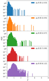 |
Fig. A.1. Redshift distribution of sources in log-space. The distributions for each bin is shown for the full range of redshifts used in this analysis. Compare with Fig. 2. |
Statistical properties of the redshift distribution of galaxies in each tomographic bin.
In Sect. 4.1 we showed our main results, focusing mainly on S8 and Σ8 constraints, where we argued that, in general, S8 does not capture the best-constrained direction perpendicular to the Ωm − σ8 degeneracy. Figure A.2 demonstrates our fitting method on band powers, which we use to find an appropriate α that captures the direction perpendicular to the degeneracy line. In the right-hand panel we show the best-fitting σ8 = Σ8(Ωm/0.3)−α (dashed curve) to the sampled σ8 and Ωm posterior points for the band powers. We find 0.58 to be the best-fit value for α. In the left-hand panel we show the resulting Σ8 and Ωm for α fixed to 0.58. Here we calculate Σ8 for each point in the samples separately. Comparing the left-hand side of this figure with Fig. 6 we see that Σ8 has smaller correlation with Ωm than S8.
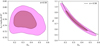 |
Fig. A.2. The best-fitting curve of the form σ8 = Σ8(Ωm/0.3)−α and its resulting Σ8. Here we demonstrate the fitting method using band powers. The dashed curve in the right-hand panel shows the best-fitting function to all samples in the σ8 and Ωm plane for which we find α = 0.58. The left-hand panel shows the resulting marginal Σ8 posterior against Ωm. |
While we showed best-fit values and credible regions for S8 and Σ8 in Sect. 4.1, here we provide credible regions for all constrained parameters in Table A.2. We note that our constraints for most parameters are prior-dominated and therefore in the case of flat priors the credible regions are affected by smoothing and the sampler reaching the edge of the prior range. In the table we report constrained parameters in bold. To assess which parameters are constrained, we consider the relative height of the 2σ levels and the maximum of a one dimensional Gaussian,
 (A.1)
(A.1)
Marginal constraints on all model parameters.
where Pr(θ) is a Gaussian distribution with mean μ and variance σ2. If the relative amplitude of the marginal distribution for a parameter between its two extremes and its maximum is smaller than 0.135 we deduce that this parameter is constrained (this is done with the binned distributions without any extra smoothing). With this criterion we see that S8 and AIA are the only two physical parameters that are constrained. We do not use this criterion for the second group of parameters, which are derived from the first group, since their prior is non-flat. We note that the Ωm constraints are also prior dominated as demonstrated in J20. The last group of parameters in Table A.2 have Gaussian priors; therefore they, by definition, pass the criterion described above. Their constraints, however, are very similar to the size of the input Gaussian priors, hence we do not show them in bold.
Figure A.3 shows marginalised credible regions for all the sampled cosmological and astrophysical parameters. We show results for COSEBIs (orange), band powers (pink) and 2PCFs (cyan). We apply a kernel density estimation (KDE) method to smooth the distributions. For parameters with poor constraints, such as Ωbh2, KDE smoothing creates artificial constraints by smoothing the edges of the distribution where it hits the limits of the flat prior range. In Fig. A.4 we show our constraints for  (see Sect. 3) and AIA. Here we have shifted the contours by the Δz values in Table 1 to centre the prior, shown in grey, on zero (dashed lines). Any shift from zero for the δz parameters is indicative of a self-calibration by the cosmic shear data. We see that the δz contours mostly recover the input prior and that δz values are consistent with zero within their 1σ marginal region. The largest deviation is found for the second tomographic bin, where we see an almost 1σ shift towards negative values, indicating a preference for a redshift distribution with a larger mean. This suggests that the shifted SOM redshift distributions have underestimated the mean of the true redshift of the galaxies in bin 2. We have seen other indications in the data for an anomaly in the distribution of the second bin. Our internal consistency tests (see Appendix B for more details) also flag the second bin as an anomaly. Nevertheless, in Fig. 7 we showed that excluding redshift bin 2 has a negligible effect on our final results.
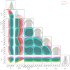 |
Fig. A.3. Constraints on sampled cosmological and astrophysical parameters. Results are shown for COSEBIs (orange), band powers (pink) and the 2PCFs (cyan). We use kernel density estimation to smooth the distributions, which in the case of poorly constrained parameters can produce artificial constraints near the prior boundaries (for example constraints on h or Ωbh2). |
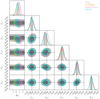 |
Fig. A.4. Constraints on δz and the intrinsic alignment amplitude AIA. The δz nuisance parameters represent our uncertainty in the mean of the redshift distributions. The input prior region is shown in grey. The prior for AIA is flat within its boundaries (the full range is between −6 and 6), while correlated Gaussian priors are used for the δz nuisance parameters (the δz priors are shifted to have a zero mean). Results are shown for COSEBIs (orange), band powers (pink) and the 2PCFs (cyan). |
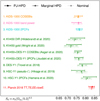 |
Fig. A.5. Comparison between S8 constraints of different surveys (extended version of Fig. 9). The top three group of bars show our KiDS-1000 results, for COSEBIs, band powers and 2PCFs. The green bars show the constraints from other cosmic shear surveys and the red ones refer to Planck 2018 results. The solid bar in each set shows the projected joint highest posterior density (PJ-HPD) credible region encompassing 68.3% of all sampled points (with the multivariate maximum posterior where determined). The dot-dashed bar displays the 1σ credible region around the maximum of the marginal distribution of S8 (Marginal HPD). For the external results we plot a third bar (dotted) showing their nominal reported values. |
In Fig. A.3 we see a mild correlation between the δz parameters and the AIA. This correlation decreases for higher redshift bins where the signal is less affected by intrinsic alignments of galaxies. Band powers show a preference for a higher AIA compared to COSEBIs and 2PCFs, with a maximum marginal value that is 0.53 larger. In our mock analysis, described in Appendix B.1, we find that a ΔAIA ≥ 0.53 occurs in about 5% of the noise realisations. We conclude that this difference is a result of the particular noise realisation in our data, given that all three summary statistics show consistent constraint for S8.
In Fig. 9 we compared the KiDS-1000 constraints to a selection of recent cosmic shear and the Planck results. In Fig. A.5 we show results for a larger selection of cosmic shear surveys and also include the reported nominal S8 constraints by each external analysis (using various estimates of central values and credible intervals). We see that the nominal results are, in all cases, very close to our estimated marginal highest density credible region. Our cosmic shear results are consistent with all the results shown here, which all report S8 values that are smaller than the inferred value from Planck.
Appendix B: Consistency tests
We perform a number of internal consistency tests on the KiDS-1000 data at the level of parameter estimates and posteriors. In Appendix B.1 we detail tests of consistency between the constraints from the three different two-point statistics. We follow the methodology of Köhlinger et al. (2019) to quantify the internal consistency between different divisions of the data based on tomographic bins (Appendix B.2). The details of the consistency test with respect to the primordial Planck results are shown in Appendix B.3. A summary of this appendix can be found in Sects. 4.3 and 4.4.
B.1. Consistency between statistics
The two-point statistics that we consider have differing sensitivities to ℓ-scales as shown in Fig. 1. Therefore, despite being measured from the exact same data set, we do not expect them to find the same constraints on cosmological parameters. Previously, seemingly incompatible results from analysis of the same data with different two-point statistics has been seen. For example, the quadratic power spectrum estimator developed by Köhlinger et al. (2017) yielded a lower value of S8 compared to the 2PCF analysis on the same KiDS data set (using Data Release 3). In addition, the HSC analysis of Hamana et al. (2020) using 2PCFs found a higher value of S8 compared to the pseudo-CL analysis of Hikage et al. (2019). Unlike these previous analyses, here we quantify the level of difference that we expect for constriants from our summary statistics.
To quantify the expected difference between 2PCFs, band powers, and COSEBIs we analyse mock data. We produce mock data by adding noise to a theoretical data vector. We draw the noise realisations from multivariate Gaussian distributions based on a cross-covariance between the different statistics. To estimate this cross-covariance we use the SALMO simulations described in Sect. 4 of J20.
In Fig. B.1 we show the cross-correlation matrix between the three two-point statistics showing combinations with redshift bins 1 and 5. We can see sub-matrices for the auto-correlations of each of the statistics, as labelled in the figure. The top triangle entries show the level of cross-correlations, while the bottom triangle shows all the values that exceed ±20% (red for positive and blue for negative values). We see that our two-point statistics have non-negligible cross-correlations, with highest values belonging to correlations between ξ− and band powers or COSEBIs. The figure also shows negative elements presenting anti-correlations. These are most pronounced in the case of COSEBIs and band powers. In addition, we see that many of the elements of the cross-covariance are small, showing a lack of correlation. For example, the small-scale ξ± is not used by the other statistics, and also COSEBIs are uncorrelated with the high-ℓ modes of the band powers.
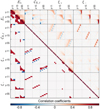 |
Fig. B.1. Cross-correlation matrix between COSEBIs (En), band powers (𝒞E,l) and 2PCFs (ξ±) from SALMO mocks. The top triangle shows the cross-correlation values corresponding to the colour-bar. The bottom triangle highlights the entries with more than 20% (red) or less than −20% (blue) correlation. We show results for tomographic bin combinations of the lowest and highest redshift bins only, resulting in three blocks per statistic containing the bin combinations 1–1, 1–5, and 5–5. |
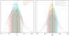 |
Fig. B.2. Distribution of inferred S8 values from 100 realisations of the data vector sampled from the covariance matrix. Left: the distribution of the maximum of the marginal distribution for S8. Results are shown for COSEBIs (orange), band powers (pink) and 2PCFs (cyan). For comparison we show a Gaussian distribution centred at the input value of S8 and a standard deviation equal to the mean of the individual standard deviations for each realisation and set of two-point statistics (grey dashed curve). Right: the difference between the S8 posterior modes of pairs of two-point statistics (as indicated in the legend) given the same noise realisation. The same reference Gaussian distribution is shown in grey (dashed curve) but centred on zero. |
With this cross-covariance we produce 100 realisations of a data vector containing COSEBIs, band powers and 2PCFs. We then divide the data vector and covariance matrix based on each set of statistics that we used in our fiducial analysis. We apply the same setup and pipeline as described in Sect. 3 to these mock data and find parameter constrains. Figure B.2 shows the resulting distribution of the maximum of the marginals for S8 (left panel). For comparison we also show a Gaussian distribution centred on the input S8 with the averaged standard deviation of all the chains. The right-hand panel shows the distribution of the difference between the S8 posterior modes shown in the left-hand panel for each pair of two-point statistics given the same noise realisation.
From the left-hand side of Fig. B.2 we can immediately see that the distribution for band powers is wider than for COSEBIs which in turn is wider than for 2PCFs. This results from the choice of α for S8, which is not perpendicular to the σ8 and Ωm degeneracy for COSEBIs and band powers. As expected, we find the maximum of the marginal distribution to be biased with respect to the input S8 (also see Sect. 6.4 of J20). 2PCFs show the smallest bias, however they also possess the tightest distribution, resulting in a similar relative bias compared to their width (see the discussion on MAP versus maximum marginal values in Sect. 4.1). On the right-hand side we see that the ΔS8 between two statistics has a comparable size to the mean distribution shown in grey. To assess the level of difference that we expect for ΔS8, we compare the width of each distribution with the mean distribution using σ values coming from the two statistics that are compared. We find that ΔS8 is only 20 − 30% tighter than its corresponding mean values, comparing any two of the statistics. This means that we do not expect to find perfect agreement between the results of different two-point statistics. In the KiDS-1000 analysis we find the largest S8 difference to be between COSEBIs and 2PCFs. Based on the analysis here we conclude that this difference of 0.4σ is expected.
To assess the fidelity of this result, we estimated a theoretical covariance between COSEBIs and 2PCFs for a non-tomographic analysis and repeated the analysis with mock data produced with the theoretical cross-covariance. We find consistent results between this test and the previous one.
Our parameter constraints for σ8 and Ωm in Fig. 6 show that the ξ± results are shifted along the degeneracy line towards high σ8 and low Ωm, such that they touch the edge of our prior range. This seemingly large effect is fully consistent with a noise fluctuation, and among the aforementioned 100 mock realisations we saw many examples with similar trends. Figure B.3 shows one such realisation. In some of the other realisations COSEBI or band power contours are shifted high along the degeneracy direction. In general, we find that the contours for poorly constrained parameters can move towards the edge of their prior range producing one-sided constraints, while shortening the marginalised posterior distributions. Given the hard cut at the prior edge, this will appear as a tighter constraint on a parameter, although it is fully dependent on the noise realisation. We see another example of this effect in the KiDS-1000 data in Fig. A.3 where the constraints on Abary with band powers appear tighter than the results of COSEBIs or 2PCFs (also see the ns constraints).
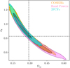 |
Fig. B.3. Marginal posterior from mock data displaying a similar degeneracy to the real KiDS-1000 data (compare with Fig. 6). The input values for σ8 and Ωm are shown with the dashed lines. These are results for one of the 100 mock realisations that we analysed. In the same set of realisations we find a number of similar results, with shortened contours for one or more of the statistics. |
B.2. Internal consistency of KiDS data
Following the methodology of Köhlinger et al. (2019), we perform three tiers of tests on divisions of the data based on splitting according to tomographic bins and all their cross-correlations. With the tier 1 test we compare the Bayesian evidence,
 (B.1)
(B.1)
where M is the model under consideration, with parameters p. The evidence is calculated for two cases: the fiducial run (1-cosmo henceforth) and an analogous run where the parameters are duplicated for each split of the data (2-cosmo henceforth). In the 2-cosmo run each part of the data has its own set of parameters to constrain, but the correlations within the data are taken into account via the data covariance matrix. We compare the evidences using the Bayes factor,
 (B.2)
(B.2)
We assume that the a priori probabilities of the two models are equal, Pr(M2) = Pr(M1). With this assumption, the Bayes factor compares the probability of the models given the data. If R < 1 then M2 is preferred by the data and vice versa. For our internal consistency test M1 is the 1-cosmo model, where all the parameters are shared between the two parts of the data and M2 is the 2-cosmo case.
We use the MONTEPYTHON package (Audren et al. 2013; Brinckmann & Lesgourgues 2018) where our internal consistency tests are developed. We find very good consistency between our MONTEPYTHON and KCAP likelihood codes (better than our 0.1σ threshold). Currently, MONTEPYTHON does not allow for sampling over parameters with non-flat priors. To circumvent this issue it is common practice to include the prior in the likelihood values. This can result in biased estimates of Z for non-flat priors. In our fiducial chains the δz shifts have a Gaussian prior (as does δc for the 2PCFs). In Sect. 4.2 we showed that fixing these to their fiducial value has little impact on the constraints (the no σz case). Given this limitation in MONTEPYTHON and the negligible impact of the δz shifts, we fix these parameters (and δc for the 2PCFs), for both 1 and 2-cosmo runs.
Given a high-dimensional parameter space, it is difficult to estimate the evidence accurately. Alternative methods to MULTINEST have been proposed which aim to provide a more reliable value for Z (e.g. POLYCHORD, Handley et al. 2015). These alternatives are however several times slower than the MULTINEST runs; thus we estimate the evidence from the MULTINEST output using two methods: the standard approach employing the posterior sample (trad.) and an importance nested sampling (import.) version generated automatically by MULTINEST. To estimate the traditional method we use the ANESTHETIC processing tool (Handley 2019). We find that in general the differences between these estimates of Z are larger than their associated errors, while it is not clear which one is closer to the truth. To assess this, we run one POLYCHORD chain for a case where we found the largest difference between the traditional and importance sampling values. We find that the POLYCHORD estimate of log10Z is in-between these two values. Therefore, we report the Bayes factor for both of these estimates.
Lemos et al. (2020) suggested using suspiciousness, S, instead of the Bayes factor for the tier 1 test, as it has much reduced sensitivity to the volume of the prior. This is particularly useful for the tier 1 test as the 2-cosmo model is inherently penalised due to the doubling of parameter space. We show lnS values for all cases, but refrain from translating them into the popular τσ measure. To do so, we need a robust estimate of the effective number of parameters, NΘ, for both the 1-cosmo and 2-cosmo runs. In Sect. 6.3 of J20 we see that the dimensionality measure which has so far been used in conjunction with suspiciousness is in general a biased estimator of NΘ. The other methods suggested in J20 involve running multiple computationally expensive chains. Therefore, here we only report the values for lnS and leave their further interpretation to future work.
With the tier 2 test we consider the posterior of the difference between the two instances of the same parameters that result from the 2-cosmo analysis. We count the fraction of samples in this distribution with lower density than the posterior density at the origin20, where the results for both sections of the data are perfectly matched. The smaller this fraction the less likely it is to have agreement between the two parts of the data. This fraction is then cast into an τσ value based on the fractional differences between the peak and the tails of a one dimensional Gaussian distribution (more details in Sect. 2.2 of Köhlinger et al. 2019).
The only fully constrained parameters with KiDS-1000 data are S8 (or Σ8) and AIA, as discussed in Appendix A. Hence, for the tier 2 tests we only consider the marginal distributions for these two parameters and their combinations.
Table B.1 lists the tier 1 results in the left columns and the tier 2 results on the right. We report values for all three two-point statistics. Similar trends can be seen for the results of COSEBIs, band powers and 2PCFs. In all cases redshift bin 2 stands out, whereas the remaining tests return values consistent with noise. In this case the tier 1 test shows a negative log10R indicating a preference for the 2-cosmo model. We use Jeffreys’ scale to interpret the significance of the measured log10R, and find it to show strong to decisive evidence for the 2-cosmo model, depending on the statistics and the method used to estimate the evidences. The tier 2 test corroborates this result. We see that the parameter differences for this separation of the data are larger than all the other cases, with up to21 3σ.
Tier 1 (left) and tier 2 (right) test results for COSEBIs, band powers (BP) and 2PCFs.
To better understand the origin of the inconsistency between the second tomographic bin and all others, we compare the translated posterior distributions (TPD, Köhlinger et al. 2019, Sect. 2.3) that are produced from the 2-cosmo chains. We make predictions for all bins using the TPDs and compare them with the data. Figure B.4 shows results for band powers. We choose band powers here as their data points are considerably less correlated compared to COSEBIs or 2PCFs, facilitating a visual inspection. The TPDs of bin 2 and its cross-correlations are shown in red, while the TPDs of all other bins are presented in blue. The width of the curves show the standard deviation of the TPDs. We see that the first bin and its cross-correlations, owing to their very low signal-to-noise, cannot distinguish between the two sets of TPDs, whereas for other pairs of redshift bins the two TPDs are clearly separated. The inconsistency of the bin 2 results with all other bins is clear here, with the former having larger signals than expected for their redshift distributions.
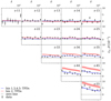 |
Fig. B.4. Band power data compared to the best-fit model from the internal consistency test that isolates all bin combinations involving the second tomographic bin. The red curves show the translated posterior distributions (TPDs) resulting from the second bin and its cross-correlations. The blue curves are the TPDs derived from the remainder of the tomographic bins and their combinations. The shaded bands around the curves show their standard deviations. |
A reasonable explanation for this discrepancy is that a small but high-redshift population of galaxies has contaminated the second bin. We expect a higher signal for higher-redshift galaxies, as their light passes more structures before reaching us producing stronger correlations between their observed shapes. Since here we have no freedom to change the redshift distributions, the model is forced to increase the amplitude of the power spectra to compensate for the higher amplitude in correlations with bin 2. This is done via varying both AIA and S8 as can be seen in Fig. B.5. This figure illustrates the tier 2 results, comparing the constraints for the parameters obtained from bin 2 and its cross-correlations (orange) with the rest of the data (blue). We show marginal distributions for the subset of parameters, σ8, Ωm and AIA. In Fig. A.4 we saw that the largest δz shift belonged to this bin. Including these shift parameters can mitigate these inconsistencies to some extent.
 |
Fig. B.5. Marginal posteriors using band powers in the internal consistency test that isolates all bin combinations involving the second tomographic bin. The test duplicates the sampling parameters (with fixed δz) and assigns them to the two parts of the data vector. The orange contours refer to the split including the second bin and all its cross-correlations, while the blue ones present the constraints from the remainder of the redshift bins (and their cross-correlations). The cross-covariance between the two parts of the data are included via the data covariance matrix. Other divisions of the data show much more consistent results. |
In Sect. 4.2 we evaluated the impact of removing the second bin from the analysis and found its effect on our final results to be negligible. Consequently, we do not exclude this bin from our fiducial analysis (also see the discussion in Sect. 4.3). Regardless, due to the excess signal in bin 2, including it in the analysis can only serves to increase the value of S8 and decrease the tension with Planck.
B.3. Quantifying tension with Planck
In Sect. 4.4 we reported the tension in the marginal distributions of S8 and Σ8 for COSEBIs. Here we use a similar methodology to the tier 1 test in Appendix B.2 to quantify the inconsistency between KiDS-1000 and Planck, also using COSEBIs, which are chosen owing to their better goodness-of-fit to the model.
We compare the evidence for a single set of cosmological parameters for both KiDS-1000 and Planck by running a joint chain (1-cosmo) with the evidences found for their separate analysis (2-cosmo). The only difference here is that the two data sets are independent, allowing us to use the respective fiducial chains for the 2-cosmo runs. The Bayes factor can now be written as,
 (B.3)
(B.3)
where M1 is the model with shared parameters between KiDS-1000 and Planck, while M2 is the model with separate parameters for KiDS (M2, K) and Planck (M2, P). We find log10R = −1.15 (strong) using evidences from importance nested sampling and log10R = −0.54 (substantial) with the standard nested sampling method, both showing a preference for M2, corresponding to a tension between KiDS-1000 and Planck. We also report the suspiciousness value, lnS = −2.94 but find a negative value for the difference between the dimensionality of the 1-cosmo and 2-cosmo runs, although we expect a positive value. As discussed in Appendix B.2, the estimated values of dimensionality are generally biased with regards to the effective number of degrees of freedom as read off from the sampling distribution of the minimum χ2. As a result we are unable to cast this result into the more intuitive τσ measure.
Appendix C: Impact of survey pixel size on the size of constraints
To calculate covariance matrices, we need to estimate the effective area, Aeff, of the observed images; see Joachimi et al. (2020), Appendix E, for the details of the covariance model. The value of Aeff depends on the assumed pixel size, since we use a binary mask. The shape noise term is independent of Aeff, since this term is estimated using the effective number of galaxy pairs. There are two other Gaussian terms in the covariance matrix which are impacted by the choice of Aeff. For the cosmic variance (also known as sample variance) and the mixed terms the covariance scales approximately with the inverse of Aeff. However, in the case of the mixed term, we include the effective number density of galaxies, neff, which in turn depends on the effective area. We scale neff with respect to Aeff to keep the total number of galaxies in each tomographic bin constant and independent of the effective area. As a result, the only Gaussian term that is impacted by Aeff is the cosmic variance term. J20 argue for using the effective area of a survey with the same extent as KiDS-1000 but without the very small scale masks to calculate this term. One way to achieve this is by lowering the resolution of the mask, as we implement here.
Figure C.1 shows marginal constraints for S8 with the fiducial priors used in our analysis. Noise-free mock data is used to assess the impact of the pixel size. We consider three different resolutions of the survey mask: at the OmegaCam pixel size, resulting in Aeff = 777.4 deg2; using HEALPIX with Nside = 4096 (Aeff = 867.0 deg2); and using HEALPIX with Nside = 2048 (Aeff = 904.2 deg2). The survey masks consider a pixel as observed, if some fraction of the sky area covered by it has unmasked imaging, which explains the increase in area as the resolution becomes coarser. Here we have kept the area for the sub-dominant non-Gaussian terms fixed to Aeff = 867.0 deg2 and included the m calibration covariance terms which are independent of the area.
 |
Fig. C.1. Impact of mask pixel size on S8 constraints with mock data. The covariance matrices are calculated using the effective areas determined with the OmegaCam pixel size (red solid), HEALPIX with Nside = 4096 (blue dotted) and HEALPIX with Nside = 2048 (green dashed). The mock data is noise free and the dashed line shows the input S8 value. |
We see that the constraints are not significantly impacted by the effective area. Both the standard deviation of the sampled points and the peaks of the marginal distributions are unchanged well within our error margin of 0.1σ. In Figs. 10 and 11 of J20 we see that the diagonal terms in the cosmic shear covariance matrix are dominated by the noise term, whereas the diagonals of the sub-matrices are dominated by the mixed term. Therefore, this result is expected. In all three cases the maximum marginal value of S8 is slightly biased towards smaller values, while the projection of the maximum posterior recovers the input.
Appendix D: Modelling residual constant c-terms
The measured ellipticities of galaxies can be biased by an additive term, usually dubbed the c-term. In our data we correct for a constant overall c-term for each of the ellipticity components (see G20 for more details). There is an uncertainty on this parameter, such that there could be some residual signal from the term that remains in the data. We are able to marginalise over this uncertainty using additional free parameters. In our analysis we considered a single additive parameter  which only affects ξ+. The other statistics that we consider are unaffected by this constant additive terms (to very good approximation in the case of band powers); however, they can still be affected by c-terms due to survey boundary effects. Here we first look at how ξ− is impacted by a constant c1 and c2, and then propagate through to COSEBIs and band powers.
Under a flat-sky approximation we can write the correlation functions as,
 (D.1)
(D.1)
where ϵa, 1 and ϵa, 2 are the Cartesian ellipticity components of a galaxy and ϕ is the polar angle of the vector connecting the two galaxies, labelled as a and b. The average is taken over all pairs of galaxies with separation angle within a defined θ-bin.
Let us assume that the observed ellipticity is only biased by the c-terms, c1 and c2, and write the observed ellipticity as,
 (D.2)
(D.2)
where i = 1, 2. We can now find the observed ξ± by replacing ϵi with  in Eq. (D.1),
 (D.3)
(D.3)
where we set ⟨ϵi⟩ = 0. For a finite field ⟨cos(4ϕ)⟩(θ) and ⟨sin(4ϕ)⟩(θ) do not vanish and their values depend on θ. Therefore, we expect to get a small contribution from the c-terms to ξ−. We note that ξ× is also similarly affected by the c-terms and an analogous equation can be written for this correlation.
Both COSEBIs and band powers are defined as integrals over ξ±, therefore we can propagate the effect of the c-terms using Eqs. (7) and (10). As a constant additive term is filtered out for these statistics, only the ξ− terms remain. First we define  . We can then write,
 (D.4)
(D.4)
and
 (D.5)
(D.5)
In practice, to marginalise over the effect of the c-terms on ξ−, COSEBIs and band powers, we need to let both c1 and c2 vary independently. Here we have assumed that the c-terms are constant within the survey and as such they can be taken out of the integrals in Eqs. (D.4) and (D.5) to yield
 (D.6)
(D.6)
and
 (D.7)
(D.7)
To model the effect of the c-terms for ξ−, we can use the position of galaxies in the data to measure the expectation value of cos(4ϕ) and sin(4ϕ), or the integrals containing them in Eqs. (D.6) and (D.7) in the case of COSEBIs and band powers. We can then use these values as inputs to model  ,
,  and
and  . This can be done by running the same tree-code used to measure the 2PCFs with two separate runs where the ellipticities of galaxies are replaced by two sets of constant values.
We estimate that this effect on COSEBIs, band powers and ξ− for the KiDS-1000 data is smaller than 1% compared to the size of the error bars, where we used values for c1 and c2 taken from the 5σ limits of their estimated errors (see G20, Sect. 3.5.1). Since ⟨cos(4ϕ)⟩(θ) and ⟨sin(4ϕ)⟩(θ) are non-zero due to survey boundaries and masks, the effect of the constant c-term is scale-dependent (increases with θ). In Fig. D.1 we show this effect for COSEBIs,  , with respect to the expected error on the measured COSEBIs through the covariance matrix Cnn, which we have used in our fiducial analysis. Here we have used a KV450 footprint and expect this effect to be even less significant if a KiDS-1000 footprint is employed.
 |
Fig. D.1. Effect of a constant additive shear bias on COSEBIs. |

For larger surveys with contiguous coverage these terms should be small given angular scales that are well within the survey area. However, the measurement errors also decrease for these surveys. Therefore, their importance needs to be re-evaluated for future surveys.
Appendix E: Distribution of the amplitude of COSEBIs in SALMO simulations
We measure COSEBI E- and B-modes from the SALMO simulations described in Joachimi et al. (2020, Sect. 4) and compare their distribution to a Gaussian with the same mean and variance using a Kolmogorov-Smirnov (KS) test. Fig. E.1 shows the p-values associated with this test. This figure can be contrasted with Fig. 17 in J20, where ξ+ shows a low p-value for its largest two θ-bins over all redshift bin combinations. The distributions of the COSEBI B-modes are consistent with Gaussiandistributions, whereas there are a few smaller p-values (shown in hues of red) for the E-modes, with a minimum of 0.01. Considering Fig. 1, we expect to get a similarly Gaussian distribution for COSEBIs as for ξ−(θmax). In the SALMO simulations the distribution of ξ− is perfectly Gaussian. The p-values for ξ+(θmax) on the other hand go as low as 10−4, therefore the significance of their non-Gaussianity is much higher.
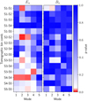 |
Fig. E.1. Distribution of COSEBI E- and B-modes in SALMO simulations, as a function of tomographic bin combination and COSEBI mode. The plot shows the p-value of a Kolmogorov-Smirnov test of the sampling distribution from 1000 mocks compared to a Gaussian. The minimum p-value that we find is 0.01, showing a marginally non-Gaussian distribution. |
Given this marginally non-Gaussian result for some of the COSEBIs modes for certain pairs of redshift bins, we test the distribution of their χ2 values in the simulations (comparing each mock En with their mean value over all mocks) and find that to be consistent with a χ2 distribution with the correct degrees of freedom (p-value = 0.8). Given these results, we conclude that the full distribution of COSEBIs is close enough to a Gaussian. For a likelihood analysis the χ2 is the quantity that is used and therefore the assumption that it is χ2-distributed is of more importance than the Gaussianity of the individual COSEBIs modes. With more simulations we can resolve whether or not the slightly low p-values persist.
Appendix F: Changes after unblinding
Our blinding strategy is described in Kuijken et al. (2015). Prior to unblinding our data, we ran all the fiducial chains using a covariance matrix calculated with the fiducial set of model parameters used in J20. Since our blinding strategy allowed for comparing relative constraints between different setups, without major changes to the conclusions, we ran all of the systematics and internal consistency chains for one of the blinds only.
After unblinding we re-ran the systematics and internal consistency chains for the correct blind without changing the cosmological parameters used in the covariance matrix. After unblinding we changed the definition of δc to take both positive and negative values and re-ran the 2PCFs chains. This update only impacted the results at a level consistent with variations between different chains.
For our fiducial results we repeated the likelihood analysis with an updated covariance model based on the best-fit parameters of Heymans et al. (2020). These chains were run after the unblinding to test the effect of an iterated covariance model, which had a negligible impact (less than 0.1σ) on our constraint of S8. The combined chain with Planck used in our external consistency test was also run after the unblinding, with the iterated covariance matrix.
All Tables
Statistical properties of the redshift distribution of galaxies in each tomographic bin.
Tier 1 (left) and tier 2 (right) test results for COSEBIs, band powers (BP) and 2PCFs.
All Figures
|
Fig. 1. Integrands of the transformation between the angular power spectrum and 2PCFs (Eq. (6)), COSEBIs (Eq. (8)) and band powers (Eq. (12)). All integrands are normalised by their maximum value. ξ± results are shown for the maximum and minimum angular separations that are used in our analysis. For COSEBIs we chose n = 1 and n = 5, showing the range of n-modes that we consider. For band powers we show all 8 bins. COSEBIs are defined on the angular range of |
| In the text | |
|
Fig. 2. The redshift distribution of galaxies in five tomographic bins. The galaxies in each bin are selected based on their best-fitting photometric redshift, zB, the range of which is shown in the legend. |
| In the text | |
|
Fig. 3. COSEBI measurements and their best fitting model (see Table A.2). We show the best-fitting theoretical prediction with a red curve ( |
| In the text | |
|
Fig. 4. Band power measurements and their best fitting model (see Table A.2). The red curves show the best fitting model fitted to the E-modes (top triangle, |
| In the text | |
|
Fig. 5. Measurements of the shear correlation functions. The best fitting curves are shown in red (see Table A.2, |
| In the text | |
|
Fig. 6. Marginalised constraints for the joint distributions of σ8 and Ωm (left), as well as S8 and Ωm (right). The 68% and 95% credible regions are shown for COSEBIs (orange), band powers (pink) and the 2PCFs (cyan). Planck (2018, TT, TE, EE+lowE) results are shown in red. |
| In the text | |
|
Fig. 7. Impact of nuisance parameter treatment and tomographic bin exclusion on Σ8 constraints. Results are shown for COSEBIs (left), band powers (centre) and 2PCFs (right), with fiducial constraints in orange, pink, and cyan, respectively. We use the best-fitting value of α for the fiducial chain of each set of statistics to define Σ8 (Eq. (14)) using the covariance matrix generated from the Tröster et al. (2020a) values instead of the iterative covariance used in Sect. 4.1. The value of α for each panel is given underneath. Two sets of credible regions are shown for each case: the multivariate maximum posterior (MAP, circle) with PJ-HPD (solid) credible interval and the maximum of the Σ8 marginal posterior (diamond) with its highest density credible interval (dot-dashed). The shaded regions follow the fiducial PJ-HPD results of the corresponding statistics. We show Planck results (red), as well as the fiducial results of the other two statistics for the given α of each panel for comparison. Cases 5–12 show the impact of different observational systematics, while cases 13 and 14 show results for the impact of astrophysical systematics. The last six cases present the effect of removing redshift bins and their cross-correlations from the analysis. |
| In the text | |
|
Fig. 8. Relative impact of nuisance parameters and the removal of redshift bins. Each of the cases explored in Fig. 7 is compared to their corresponding fiducial results. COSEBIs are shown as orange circles, band powers as pink crosses and 2PCFs as cyan squares. Left: the difference between the upper edge of the marginal Σ8 posterior for each case and its fiducial chain, normalised by half of the length of the marginal credible interval of the case. The grey shaded area indicates the region in which systematic shifts remain below the 1σ statistical error. Right: comparison of constraining power between the fiducial and the other cases. Here α is fitted to each chain separately to find the tightest Σ8 = σ8(Ωm/0.3)α constraint for each case. We show the fractional difference between the standard deviations of the case and the fiducial one. |
| In the text | |
|
Fig. 9. Comparison between S8 values for different surveys. All results are shown for both multivariate maximum posterior (MAP) and PJ-HPD (upper solid bar), as well as the marginal mode and the marginal S8 credible interval (lower dot-dashed bar). The top three points show our fiducial KiDS-1000 results. The next four show a selection of recent cosmic shear analyses from external data as well as previous KiDS data releases. We note that S8 does not fully capture the degeneracy direction for all of the analysis above (see the discussion in Sect. 4.1 and Appendix A). For example for the HSC-Y1 contours α = 0.45 was found to be the best fitting power. The last entry shows the Planck 2018 (TT, TE, EE+lowE) constraints. An extended version of this plot can be found in Appendix A. |
| In the text | |
|
Fig. 10. Comparison between KiDS-1000 and other surveys in the S8 − Ωm plane. The fiducial KiDS-1000 results which use COSEBIs (orange) and the Planck primary anisotropy constraints (red) are shown in both panels. The DES-Y1 results of Troxel et al. (2018b, purple) and HSC-Y1 results of Hikage et al. (2019, grey) are shown in the left panel, while the KV450 constraints of Wright et al. (2020a, green) and the joint KV450 and DES-Y1 results of Asgari et al. (2020, blue) are shown in the right panel. A summary of these constraints in S8 can be found in Fig. 9. |
| In the text | |
|
Fig. A.1. Redshift distribution of sources in log-space. The distributions for each bin is shown for the full range of redshifts used in this analysis. Compare with Fig. 2. |
| In the text | |
|
Fig. A.2. The best-fitting curve of the form σ8 = Σ8(Ωm/0.3)−α and its resulting Σ8. Here we demonstrate the fitting method using band powers. The dashed curve in the right-hand panel shows the best-fitting function to all samples in the σ8 and Ωm plane for which we find α = 0.58. The left-hand panel shows the resulting marginal Σ8 posterior against Ωm. |
| In the text | |
|
Fig. A.3. Constraints on sampled cosmological and astrophysical parameters. Results are shown for COSEBIs (orange), band powers (pink) and the 2PCFs (cyan). We use kernel density estimation to smooth the distributions, which in the case of poorly constrained parameters can produce artificial constraints near the prior boundaries (for example constraints on h or Ωbh2). |
| In the text | |
|
Fig. A.4. Constraints on δz and the intrinsic alignment amplitude AIA. The δz nuisance parameters represent our uncertainty in the mean of the redshift distributions. The input prior region is shown in grey. The prior for AIA is flat within its boundaries (the full range is between −6 and 6), while correlated Gaussian priors are used for the δz nuisance parameters (the δz priors are shifted to have a zero mean). Results are shown for COSEBIs (orange), band powers (pink) and the 2PCFs (cyan). |
| In the text | |
|
Fig. A.5. Comparison between S8 constraints of different surveys (extended version of Fig. 9). The top three group of bars show our KiDS-1000 results, for COSEBIs, band powers and 2PCFs. The green bars show the constraints from other cosmic shear surveys and the red ones refer to Planck 2018 results. The solid bar in each set shows the projected joint highest posterior density (PJ-HPD) credible region encompassing 68.3% of all sampled points (with the multivariate maximum posterior where determined). The dot-dashed bar displays the 1σ credible region around the maximum of the marginal distribution of S8 (Marginal HPD). For the external results we plot a third bar (dotted) showing their nominal reported values. |
| In the text | |
|
Fig. B.1. Cross-correlation matrix between COSEBIs (En), band powers (𝒞E,l) and 2PCFs (ξ±) from SALMO mocks. The top triangle shows the cross-correlation values corresponding to the colour-bar. The bottom triangle highlights the entries with more than 20% (red) or less than −20% (blue) correlation. We show results for tomographic bin combinations of the lowest and highest redshift bins only, resulting in three blocks per statistic containing the bin combinations 1–1, 1–5, and 5–5. |
| In the text | |
|
Fig. B.2. Distribution of inferred S8 values from 100 realisations of the data vector sampled from the covariance matrix. Left: the distribution of the maximum of the marginal distribution for S8. Results are shown for COSEBIs (orange), band powers (pink) and 2PCFs (cyan). For comparison we show a Gaussian distribution centred at the input value of S8 and a standard deviation equal to the mean of the individual standard deviations for each realisation and set of two-point statistics (grey dashed curve). Right: the difference between the S8 posterior modes of pairs of two-point statistics (as indicated in the legend) given the same noise realisation. The same reference Gaussian distribution is shown in grey (dashed curve) but centred on zero. |
| In the text | |
|
Fig. B.3. Marginal posterior from mock data displaying a similar degeneracy to the real KiDS-1000 data (compare with Fig. 6). The input values for σ8 and Ωm are shown with the dashed lines. These are results for one of the 100 mock realisations that we analysed. In the same set of realisations we find a number of similar results, with shortened contours for one or more of the statistics. |
| In the text | |
|
Fig. B.4. Band power data compared to the best-fit model from the internal consistency test that isolates all bin combinations involving the second tomographic bin. The red curves show the translated posterior distributions (TPDs) resulting from the second bin and its cross-correlations. The blue curves are the TPDs derived from the remainder of the tomographic bins and their combinations. The shaded bands around the curves show their standard deviations. |
| In the text | |
|
Fig. B.5. Marginal posteriors using band powers in the internal consistency test that isolates all bin combinations involving the second tomographic bin. The test duplicates the sampling parameters (with fixed δz) and assigns them to the two parts of the data vector. The orange contours refer to the split including the second bin and all its cross-correlations, while the blue ones present the constraints from the remainder of the redshift bins (and their cross-correlations). The cross-covariance between the two parts of the data are included via the data covariance matrix. Other divisions of the data show much more consistent results. |
| In the text | |
|
Fig. C.1. Impact of mask pixel size on S8 constraints with mock data. The covariance matrices are calculated using the effective areas determined with the OmegaCam pixel size (red solid), HEALPIX with Nside = 4096 (blue dotted) and HEALPIX with Nside = 2048 (green dashed). The mock data is noise free and the dashed line shows the input S8 value. |
| In the text | |
|
Fig. D.1. Effect of a constant additive shear bias on COSEBIs. |
| In the text | |
|
Fig. E.1. Distribution of COSEBI E- and B-modes in SALMO simulations, as a function of tomographic bin combination and COSEBI mode. The plot shows the p-value of a Kolmogorov-Smirnov test of the sampling distribution from 1000 mocks compared to a Gaussian. The minimum p-value that we find is 0.01, showing a marginally non-Gaussian distribution. |
| In the text | |
Current usage metrics show cumulative count of Article Views (full-text article views including HTML views, PDF and ePub downloads, according to the available data) and Abstracts Views on Vision4Press platform.
Data correspond to usage on the plateform after 2015. The current usage metrics is available 48-96 hours after online publication and is updated daily on week days.
Initial download of the metrics may take a while.