| Issue |
A&A
Volume 641, September 2020
|
|
|---|---|---|
| Article Number | A171 | |
| Number of page(s) | 31 | |
| Section | Extragalactic astronomy | |
| DOI | https://doi.org/10.1051/0004-6361/202037868 | |
| Published online | 29 September 2020 | |
Double-peak emission line galaxies in the SDSS catalogue
A minor merger sequence
1
Sorbonne Université, LERMA, Observatoire de Paris, PSL research university, CNRS, 75014 Paris, France
2
RWTH Aachen University, Institute for Theory of Science and Technology, Aachen, Germany
e-mail: This email address is being protected from spambots. You need JavaScript enabled to view it.
3
Institut d’Astrophysique de Paris (UMR 7095: CNRS & Sorbonne Université), 98bis bd Arago, 75014 Paris, France
4
Center for Astrophysics – Harvard and Smithsonian, 60 Garden St. MS09, Cambridge, MA 02138, USA
5
Sternberg Astronomical Institute, M.V. Lomonosov Moscow State University, 13 Universitetsky prospect, Moscow 119991, Russia
6
New York University Abu Dhabi, Saadiyat Island, PO Box 129188, Abu Dhabi, UAE
Received:
2
March
2020
Accepted:
23
July
2020
Abstract
Double-peak narrow emission line galaxies have been studied extensively in the past years, in the hope of discovering late stages of mergers. It is difficult to disentangle this phenomenon from disc rotations and gas outflows with the sole spectroscopic measurement of the central 3″. We aim to properly detect such galaxies and distinguish the underlying mechanisms with a detailed analysis of the host-galaxy properties and their kinematics. Relying on the Reference Catalogue of Spectral Energy Distribution, we developed an automated selection procedure and found 5663 double-peak emission line galaxies at z < 0.34 corresponding to 0.8% of the parent database. To characterise these galaxies, we built a single-peak no-bias control sample (NBCS) with the same redshift and stellar mass distributions as the double-peak sample (DPS). These two samples are indeed very similar in terms of absolute magnitude, [OIII] luminosity, colour-colour diagrams, age and specific star formation rate, metallicity, and environment. We find an important excess of S0 galaxies in the DPS, not observed in the NBCS, which cannot be accounted for by the environment, as most of these galaxies are isolated or in poor groups. Similarly, we find a relative deficit of pure discs in the DPS late-type galaxies, which are preferentially of Sa type. In parallel, we observe a systematic central excess of star formation and extinction for double peak (DP) galaxies. Finally, there are noticeable differences in the kinematics: The gas velocity dispersion is correlated with the galaxy inclination in the NBCS, whereas this relation does not hold for the DPS. Furthermore, the DP galaxies show larger stellar velocity dispersions and they deviate from the Tully-Fisher relation for both late-type and S0 galaxies. These discrepancies can be reconciled if one considers the two peaks as two different components. Considering the morphological biases in favour of bulge-dominated galaxies and the star formation central enhancement, we suggest a scenario of multiple, sequential minor mergers driving the increase of the bulge size, leading to larger fractions of S0 galaxies and a deficit of pure disc galaxies.
Key words: galaxies: kinematics and dynamics / galaxies: interactions / galaxies: general / galaxies: irregular / techniques: spectroscopic / methods: data analysis
© D. Maschmann et al. 2020
 Open Access article, published by EDP Sciences, under the terms of the Creative Commons Attribution License (https://creativecommons.org/licenses/by/4.0), which permits unrestricted use, distribution, and reproduction in any medium, provided the original work is properly cited.
1. Introduction
The evolution of galaxies over cosmic time is largely determined by their mass growth and is thus connected to their environment and their merger rate. It is well observed that the mix of morphological types of galaxies depends on the environment (Dressler 1980; Whitmore et al. 1993). The star formation rate (SFR) of galaxies is a well-suited diagnostic to characterise their evolutionary state. Galaxies can, on the one hand, enhance their star formation rate through interaction with their environment (Bothun & Dressler 1986; Pimbblet et al. 2002), but, on the other hand, they can also be quenched by the environment (Balogh et al. 1998). Isolated galaxies are thought to refuel their discs with gas from extended halos and from cosmic filaments, while galaxies located in massive clusters will evolve passively (Balogh et al. 1998). The assembly and growth of galactic discs and galaxies in general are some of the key issues of galaxy simulations (e.g. Mo et al. 1998). Accretion from filaments is motivated by numerical simulations (e.g. Bond et al. 1996), while observational detection is based on filaments of galaxies in cluster environments (e.g. Laigle et al. 2018; Sarron et al. 2019) and the Lyα forest tomography (e.g. Lee et al. 2018). The latter approach is the only one that directly detects so-called gas accretion.
The identification of merging galaxies is usually based on morphology (e.g. Lotz et al. 2004) or detection of dynamically close pairs (e.g. De Propris et al. 2005). Relying on the latter technique, Ellison et al. (2008) identified 1716 galaxies with companions in the Sloan Digital Sky Survey (SDSS) Data Release (DR) 4 with stellar mass ratios between 0.1 < M1/M2 < 10. Further studies of this sample found that star formation due to galaxy interactions can be triggered in low-to-intermediate density environments (Ellison et al. 2010). By extending their search to SDSS DR7, they increased their sample to 21 347 galaxy pairs and found evidence for a central starburst induced by galaxy interactions (Patton et al. 2011). By including quasi stellar objects (QSO) in their search, Ellison et al. (2011b) found that active galactic nuclei (AGN) activity can occur well before the final merging of a galaxy pair and is accompanied by ongoing star formation.
The original prediction that merging should go up to the black hole coalescence (e.g. Begelman et al. 1980) has not been observed yet. But earlier steps have been explored, and several dual AGNs, which is a late stage of a galaxy merger (Genzel et al. 2001; Koss et al. 2016, 2018; Goulding et al. 2019), or even a triple nucleus (Deane et al. 2014; Pfeifle et al. 2019), have been detected. While about 40% of ultra-luminous infrared galaxies exhibit a double nucleus (Cui et al. 2001), Koss et al. (2018) discuss that gas-rich luminous AGNs are often hidden mergers. Green et al. (2010) were first to identify a galaxy merger resulting in a binary quasar with a projected separation of 21 kpc and a radial velocity difference of 215 km s−1. Mergers with a binary quasar have also been associated with an offset and/or DP [OIII]λ5008 emission line (e.g. Comerford et al. 2009, 2013). Many systematic searches for dual AGNs have been conducted at different wavelengths (Liu et al. 2011, 2013; Koss et al. 2012; Fu et al. 2015) to discuss the nature of dual AGNs.
Using the direct detection of DP narrow emission lines, Wang et al. (2009), Liu et al. (2010), Smith et al. (2010), and Ge et al. (2012) selected large galaxy samples from several galaxy surveys. In most of these works, the search for double-peak emission lines are motivated by the search for dual AGNs or dual galactic cores. Starting from such samples, Comerford et al. (2012) conducted long-slit observations on double-peak emission line galaxies to find kiloparsec-scale spatial offsets and to constrain the selection of dual AGNs. Using the Hubble Space Telescope and the space based X-ray telescope Chandra, Comerford et al. (2015) confirmed a dual AGN, with a separation of 2.2 kpc, resulting from an extreme minor merger (460:1) creating a DP [OIII]λ5008 emission line. Follow-up observations with the Very Large Array enabled the detection of three dual AGNs, AGN wind-driven outflows, radio-jet driven outflows, and one rotating narrow-line region producing DP narrow emission lines (Müller-Sánchez et al. 2015). Long-slit observations of DP galaxies enable them to distinguish between AGN-driven outflows and a rotating disc (Nevin et al. 2016), as further supported by Monte Carlo simulations in Nevin et al. (2018). Furthermore, Comerford et al. (2018) associated double-peak emission line galaxies with galaxy mergers, concluding that at least 3% of galaxies with DP narrow AGN emission lines found in the SDSS spectra are galaxy mergers identified in SDSS snapshots.
In this article, we build an objective selection procedure for DP narrow emission line galaxies to test whether we can identify different merger stages. We did not constrain our search to dual AGNs candidates and we dis not include a visual selection in contrast to previous galaxy samples. We based our work on the value-added Reference catalogue of Spectral Energy Distributions (RCSED; Chilingarian et al. 2017).
This work is organised as follows. In Sect. 2, we describe the pipeline developed to automatically select galaxies with spectra exhibiting double-peak emission lines and describe the selection of a no-bias control sample (NBCS). Section 3 classifies this double-peak sample (DPS) relying on ionisation diagrams and on morphology and compare it with previous works. In Sect. 4, we analyse the properties of the DPS and compare them with the NBCS. In Sect. 5, we discuss our results followed by a conclusion in Sect. 6.
A cosmology of Ωm = 0.3, ΩΛ = 0.7 and h = 0.7 is assumed in this work.
2. Detection of double-peak emission line galaxies in RCSED catalogue
2.1. Spectroscopic data
The RCSED contains 800 299 galaxies selected from the SDSS DR7 spectroscopic sample (with a spectral resolving power R = 1500…2500) in the redshift-range 0.007 < z < 0.6 (Chilingarian et al. 2017). This catalogue provides k-corrected photometric data in the ultraviolet, optical, and near-infrared bands observed by the Galaxy Evolution Explorer (GALEX), SDSS, and the UK Infrared Telescope Deep Sky Survey (UKIDSS).
The RCSED catalogue also provides optical SDSS spectra in 3-arcsec circular apertures up to a magnitude limit of r = 17.77 mag (Abazajian et al. 2009) and a best-fitting template. The template assumes either a simple stellar population (SSP) model or an exponentially declining star formation history (EXP-SFH; Chilingarian et al. 2017). The best-fitting template subtracted from an original spectrum provides an emission line spectrum in the observed wavelength range [3600 Å, 6790 Å]. In Fig. 1, we show major emission lines extracted from stellar continuum subtracted spectra of three different galaxies, studied in this article as they exhibit double-peak emission lines as described in Sect. 2.2.
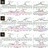 |
Fig. 1. Emission lines of three DP galaxies, namely Hβλ4863, [OIII]λ5008, [OI]λ6302, [NII]λ 6550, Hαλ6565, [NII]λ 6585, [SII]λ6718 and [SII]λ 6733. For each panel, we display on the top left, the 62″ × 62″ SDSS snapshot. Each displayed line is fitted with a double Gaussian function as explained in Sect. 2.2. We show the blueshifted Gaussian component as blue lines and the redshifted component as red lines. The green line is a superposition of the two Gaussian components. Below each emission line we show residuals. We flag lines with a confirmed DP selected with criteria described in Sect. 2.2 as “with DP” and flag the others as “no DP” for failing the criteria. The black dashed vertical line indicates the position of the stellar velocity of the host galaxy, computed by Chilingarian et al. (2017). The top spectra are for a face-on spiral galaxy at a redshift of z = 0.02 with a ΔvDP = 232 km s−1, which resembles an outflow (discussed in Sect. 5.6). The middle spectra are for an elliptical galaxy at z = 0.05 showing a ΔvDP = 495 km s−1. The bottom spectra are for a galaxy merger at z = 0.05 and ΔvDP = 269 km s−1. This is one of 58 galaxies discussed in Maschmann & Melchior (2019) showing a DP structure probably associated with recent galaxy merger. |
In the RCSED catalogue, each emission line spectrum was fitted with two different functions: (1) a Gaussian function and (2) a non-parametric distribution. In case (1), two Gaussian functions were adjusted to all allowed and all forbidden transitions. The case (2) is based on an algorithm, which adapted an arbitrary shape to all emission lines simultaneously, again grouped by the transition type. The non-parametric fit is able to fit complex line shapes such as a DP and AGN-driven outflows, and can also reveal low-luminosity AGN broad line components (Chilingarian et al. 2018). The catalogue provides the fluxes resulting from these two procedures for several emission lines, χ2 per number degree of freedom (Ndof), hereafter  , the equivalent width (EW) and other parameters, as specified in Chilingarian et al. (2017).
2.2. Automated selection procedure
We developed an automated three-stage selection procedure to find DP galaxies. The first stage pre-selects galaxies with a threshold on the S/N, and performs successively the emission line stacking, line adjustments and empirical selection criteria. Some emission lines are individually fitted at the second stage to select first DP candidates. We also selected candidates showing no DP properties to be the control sample (CS). Stages 1 and 2 are summarised in Fig. 2. At the third stage, we obtained the final DPS using the fit parameter of each line, as shown in Fig. 3. Hereafter, we explain in detail each step of the selection procedure.
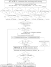 |
Fig. 2. Flowchart describing the first two stages of the automated selection procedure, detailed in Sect. 2.2. We list up all selection criteria and note the number of galaxies at each selection step. In stage 1 we select preliminary candidates and a control sample (CS) using emission line properties and χ2 ratios from emission line fitting computed by Chilingarian et al. (2017). We visualise the stacking and fitting procedure and all selection criteria described in Sect. 2.2.2. In stage 2 we describe the individual fitting of each emission line and list up all criteria for the DP flag detailed in Sect. 2.2.4. We finally select 7479 DP candidates and 89 412 galaxies for the CS. |
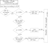 |
Fig. 3. Stage 3 of the selection procedure to find the final DPS. This algorithm sorts the fitted emission lines according to their S/N and uses the DP flags indicating confirmed DP in the specific line. All selected galaxies must have a confirmed DP in the strongest line. If the object has more than 1 (resp. 2) confirmed line(s), we must also find a DP in the second (resp. second and third) strongest line. This procedure excludes objects which have a falsely confirmed DP in some weaker lines. We finally get the DPS counting 5663 galaxies. In Table 1, we present the distribution of DP galaxies for different number of confirmed DP. |
2.2.1. Preliminary candidates
We first restricted the analysis to galaxies with detectable emission lines, in order to define a preliminary sample on which a subsequent emission line fitting can be applied. Hence, we selected objects with a S/N > 10 in the [OIII]λ5008 or Hαλ6565 lines. To secure the detection of the S[II]λ6718 and S[II]λ6733 lines within the spectra bandwidth, we added the condition z < 0.34. We thus kept a sample containing 276 239 objects from the RCSED catalogue.
We then selected 189 152 galaxies, which have a S/N > 5 in at least three emission lines among Hαλ6565, Hβλ4863, Hγλ4342, [OIII]λ5008, [OI]λ6302, [NII]λ6550, and [NII]λ6585. As described above, the non-parametric fit adapts to the line shape and is thus able to fit a DP structure. It is hence possible to disentangle single Gaussian profiles from non-Gaussian profiles. With the reduced  value of the single Gaussian and non-parametric RCSED fit, we can compared the spectra whose emission lines resemble a Gaussian shape with those spectra showing an unlikely Gaussian shape, such as a DP. We selected 99 740 galaxies with a larger
  value for the Gaussian fit than for the non-parametric fit. They were classified as preliminary candidates. Spectra with a larger
  value for the non-parametric fit were selected as the control sample (CS), since they have more likely a Gaussian shape (see detailed description in Sect. 2.2.3).
2.2.2. Emission line stacking and fitting procedure
The emission line fittings performed in the RCSED catalogue is separated for Balmer and forbidden emission lines since they can originate from different parts of the galaxy (Chilingarian et al. 2017). For the preliminary selected galaxies, we only find ∼1% showing a deviation greater than the SDSS spectral resolution between the two fits regarding the emission line position or dispersion. The RCSED catalogue has also excluded SDSS objects classified as quasars or Seyfert 1 (Schneider et al. 2010) since the stellar population analysis or the k-correction (e.g. Chilingarian et al. 2010b) is not supporting these kind of objects (Chilingarian et al. 2017). Hence, most broad-line galaxies were not included and we were not investigating such line shapes in this study.
We can thus assume a priori the same or a similar shape in all emission lines. This motivates a stacking procedure of the different emission lines of each spectra. While the shape of a single emission line can be distorted by noise, genuine signals will be enhanced in the stacked spectra characterised by a reduced noise. To guarantee the significance of this procedure, we required S/N > 5 for all stacked emission lines. To stack the emission lines, we selected each emission line in the range of ±30 Å with respect to the emission line position and transformed it into velocities. We calculated the velocity of each wavelength bin i as vi = c (Δλi)/λrest, where Δλi is the difference between the wavelength of the bin i and the observed emission line position and λrest its rest-frame wavelength. We calculated the stacked spectra by summing the flux of each selected emission line in each velocity bin vi and add the uncertainties quadratically.
We isolated the Hαλ6565, [NII]λ6550 and [NII]λ6585 emission lines for the stacking procedure. They can overlap and cause artefacts in the stacked spectra. The [NII]λ6550, λ6585 doublet is characterised by a fixed flux ratio of [NII]λ6585/[NII]λ6550 = 2.92 ± 0.32 (Acker et al. 1989). Using the non-parametric emission line fit from RCSED we could extrapolate and subtract the [NII] doublet, as done in Schirmer et al. (2013).
We fitted a single Gaussian function (gsingle) and a double Gaussian function (gdouble) against each stacked spectrum. We used the following functions for the adjustments:
 (1)
(1)
where A is the amplitude, μ the mean and σ the standard deviation of the Gaussian function, v the velocity and B a constant accounting for the background noise level.
 (2)
(2)
In Eq. (2), we used the same notation as Eq. (1) with subscripts (1, 2) defining the first and second Gaussian components. All fitting procedures were performed using the data analysis framework ROOT1
We then applied criteria to select DP candidates with the fit procedure, as follows:
-
1/2.5 < A1/A2 < 2.5
-
ΔvDP = |μ2 − μ2|> 3 δv
-
F-test.
Criteria (1) ensures that one of the two possible peaks is not suppressed or does not represent only noise. Criteria (2) demands the separation of the two peaks to be three times greater than δv, the bin-width of the spectroscopic observation, transformed into a velocity, which is 3δv = 207 km s−1. The F-test of criteria (3) directly compares the two fitted models and demands a significant decrease in χ2 relative to the increase in the Ndof for the double Gaussian fit (subset “d”) in comparison to the single Gaussian fit (subset “s”). Following Mendenhall & Sincich (2011), we calculated the F-statistic, as follows:
 (3)
(3)
and demanded the Fisher-distribution F to reject the single Gaussian hypothesis with a probability of less than 5% by using the cumulative distribution function:
 (4)
(4)
With these criteria, we selected 7479 galaxies.
The Gaussian velocity dispersions σi that we measured directly from the spectra need to be corrected for the instrumental broadening σinst (as e.g. discussed in Woo et al. 2004). We calculated the corrected dispersion as  , where σi corresponds to σ, σ1 and σ2. The resolution of the SDSS spectra is not constant for the covered wavelength range and decreases towards higher wavelengths. To correct the stacked-spectra velocity dispersions, we used the mean σinst computed over the selected emission lines. We find a mean σinst = 61 ± 4 km s−1. In the subsequent analysis, we only discussed corrected velocity dispersions.
2.2.3. Control sample selection
For later analysis, we selected a Control Sample (CS) to compare with our DPS. This sample was selected during the first stage and corresponds to galaxies showing no evidence of any DP feature. The preliminary sample, selected in Sect. 2.2.1, contains 189 152 galaxies, and was then divided into two subsamples using the Gaussian and the non-parametric fits provided in the RCSED. We kept spectra exhibiting a larger  value for the non-parametric than for the Gaussian fit to select galaxies showing Gaussian shaped emission lines. With this criterion, we selected 89 412 galaxies, building up the CS. Since we considered the same S/N thresholds for emission lines and the same maximal redshift as for the DP candidates, this is a representative control sample. Nevertheless, as further discussed in Sect. 2.3, this CS still shows a selection bias in the redshift and stellar mass distributions, and a no-bias control sample (NBCS) is selected.
2.2.4. Individual emission line fitting
In the second stage of the selection procedure, we examined the following emission lines separately: Hγλ4342, Hβλ4863, [OIII]λ5008, [OI]λ6302, [NII]λ 6550, Hαλ6565, [NII]λ6585, [SII]λ6718, and [SII]λ6733. We fitted a single and a double Gaussian function to each line. For the double Gaussian function, we set the parameters μ1, 2 and σ1, 2 provided by the best fit of the stacked emission lines (see Sect. 2.2.2) and let them vary only inside their uncertainty range ±Eμ1, 2 and ±Eσ1, 2. The uncertainties are usually smaller than the spectral bin size δλ of the SDSS which means that these values are quasi fixed. In the case of uncertainties larger than 0.4 × δλ, we fixed them to 0.4 × δλ.
Using the best fit results of the single and double Gaussian fit functions, we applied the following criteria to flag each line if we detect a DP:
-
A1, A2 > 3 σb
-
 (single) >
  (double)
 -
1/3 < A1/A2 < 3
-
S/N > 5
where σb is the root mean square (RMS) of the background noise level measured on both sides of the emission line. The first criterion ensures that the amplitude of each DP component is significantly larger than the background noise. The second criterion constrains that the double Gaussian function is better fitting the data than the single Gaussian one. With the third criterion, we excluded emission lines where one DP component is suppressed. In this case, it is likely that the weak component represents noise or an artefact of a clumpy line shape. Maschmann & Melchior (2019) discussed genuine cases where one of the components is weak or suppressed despite a high S/N. Criteria four ensures that the fitted lines are detectable and are not just noise.
For those lines showing a DP according to the selection criteria above, we set a flag to highlight the specific line as a DP line.
2.2.5. Final selection of double-peak galaxies
In the third stage of the selection procedure, we excluded galaxies which do not show any DP in the strongest emission lines which are mostly misclassified due to an artificial DP structure created by the stacking procedure. This third-stage selection is illustrated in Fig. 3.
We kept spectra with the strongest line flagged as DP. In cases of two (resp. more than two) emission lines flagged as DP, we also demanded the second (resp. second and third) strongest line to be flagged as DP. With these criteria, we excluded 1816 galaxies, which do not show a DP in their strong lines. This can occur for different reasons: (1) the fitting procedure can fail at specific lines because of a noisy line shape, (2) the spectra show only a DP structure in the stacked spectra but not in any individual line, or (3) DP occur only in weak lines, which are dominated by noise.
Our final DPS contains 5 663 galaxies with Δv = |μ2 − μ1| between 211 and 582 km s−1. In Fig. 4, we show distributions of the flux ratios between the two fit components of the Hαλ6565, [OIII]λ5008, Hβλ4863 and [NII]λ6585 emission lines. There is a noticeable difference between the flux ratio ϕmax/ϕmin of Hα and [OIII]. We also present the distribution of ΔvDP and the measured ratio of the amplitudes and velocity dispersions σmax/σmin of the two components in the stacked spectra.
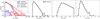 |
Fig. 4. Characteristics of the galaxies selected with a DP feature in their emission lines. From left to right: first panel: flux ratio ϕmax/ϕmin of the stronger line divided by the weaker line for the individual emission lines Hαλ6565, [OIII]λ5008, Hβλ4863 and [NII]λ6585. We display the Hαλ6565 and [OIII]λ5008 emission line ratios of the objects found in Maschmann & Melchior (2019) with blue and re hatched surfaces. The other panels display parameters computed on the stacked spectra (see Sect. 2.2.2). Second panel: velocity difference Δv between the two peak components taken from the stacking procedure. Third (resp. fourth) panel: amplitude (resp. velocity dispersion) ratio of the stronger and weaker line components of the stacked spectra. |
The number of confirmed DP lines varies between one and nine and is presented in Table 1. 92% (resp. 72%) of the selected galaxies exhibit three (resp. four) or more double-peak emission lines.
DPS sorted into groups of number of confirmed DP lines.
The automated selection procedure selected DP galaxies with an objective algorithm. This means that we did not need any visual inspection, which would have been a subjective factor in the sample selection. We show in Table 2 some fitting parameters of the first five galaxies of our DPS.
Double-peak galaxy sample.
2.3. No-bias control sample
Figure 5 displays stellar mass (Kauffmann et al. 2003) as a function of redshift for the CS and for the DPS. We can observe that very few low-redshift objects are present in the DPS. This is obviously a selection bias: our method ends up excluding small systems with M* < 1010 M⊙. This is due to the fact that we cut ΔvDP < 211km s−1: those two quantities are related through the Tully Fisher relation (Tully & Fisher 1977), as further discussed in Sect. 4.3.4. We thus indirectly cut on the redshift and the fibre size. Hence, most DP detections correspond to a fibre size larger than 3 kpc and massive galaxies which have M* > 1010.4 M⊙. The maximal redshift observed in the DPS is z = 0.32 (but this particular galaxy has no stellar mass approximation and is thus not represented in Fig. 5). Only < 1% of the DP galaxies have a redshift z > 0.25. This can be explained by the S/N cut of emission lines in the selection procedure (see Sect. 2.2.1). For comparison purposes, we defined a sample of ordinary galaxies showing no double-peak emission lines but following the same redshift and stellar mass distribution as the DPS. We randomly selected galaxies from the CS (defined in Sect. 2.2.3) following the same redshift-stellar mass distribution as the DPS. Therefore, we divided the redshift-stellar mass space into a grid of 20 × 20 boxes and randomly draw galaxies from the CS in each box, following the probability of finding a DP galaxy in the specific box. We were thus able to select 5128 galaxies from the CS as shown in Fig. 6. In order to keep the same redshift-stellar mass distribution for the NBCS as the DPS, it is not possible to exceed 5128 galaxies in the NBCS. This new sample has approximately the same redshift and stellar mass properties as the DPS but shows single Gaussian shaped emission lines and is hereafter called the no-bias control sample (NBCS). We present the redshift and stellar mass distributions for both samples in Fig. 6.
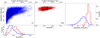 |
Fig. 5. Stellar mass-redshift distribution for the CS (blue, top left panel) and the DPS (red, top middle panel). The contours indicate the density level. In the top right panel, we show the histogram of stellar masses and, on the bottom left panel, the histogram of redshifts. We also display the fibre diameter corresponding to 3″ on top of the upper left and middle panels. |
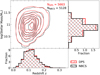 |
Fig. 6. Stellar mass-redshift distribution (see Fig. 5) for the DPS (red) and the NBCS (black). The selection of the NBCS is explained in Sect. 2.3. We also compute histograms for the redshift and the stellar mass for both samples for a better comparison. The NBCS follows the same distribution as the DPS and contains 5128 galaxies. |
2.4. Comparison with other works on DP
In this Section, we compare our DPS with previous samples. In Table 3, we cross-identify our samples at different selection steps with four other works, which released galaxy samples defined with DP galaxies or asymmetric features. Namely, we present a comparison with the samples found by Wang et al. (2009) and Liu et al. (2010), which comprise 87 and 167 Type two DP AGNs detected with the [OIII]λ5008 line. The sample of Smith et al. (2010) comprises 148 quasars classified as type one and type two AGNs. Ge et al. (2012) conducted a much broader selection procedure and provide two samples: one composed of 3030 galaxies with double-peak emission lines (hereafter G12-DP) and a second one gathering 12 582 galaxies with top flat or asymmetric line shapes (hereafter G12-TFAS).
Comparison of our DPS to other similar works with respect to the selection procedure of this work.
Our DP detection algorithm is based on a stacking procedure, which enables to study galaxies with at least three significant emission lines including a strong [OIII]λ5008 or Hαλ6565 line. These requirements are encoded among others in the preliminary selection (see Sect. 2.2.1). By comparing the sample of our preliminary candidates of 99 740 galaxies (see Sect. 2.2.1), we detect 71% (resp. 57%) of the sample found by Wang et al. (2009) (resp. Liu et al. 2010). Those galaxies, which fail our DP detection algorithm, show mostly different emission line shapes between the [OIII]λ5008 and Hαλ6565 lines. Those galaxies were then systematically sorted out in stage three of our selection procedure (see Sect. 2.2.5). We find only one DP galaxy in the RCSED catalogue selected by Smith et al. (2010), which also fails our final selection procedure due to an irregular Hαλ6565 shape where the algorithm is not able to adjust a double Gaussian function with fixed μ1, 2 and σ1, 2 (see Sect. 2.2.5). These are studies based on AGN quasars (Schneider et al. 2010) which were excluded from both the RCSED (Chilingarian et al. 2017) and our present study.
By comparing our work to the catalogues provided by Ge et al. (2012), we find a detection rate of 75% (resp. 47%) for the G12-DP (resp. G12-TFAS) sample of those detected in our preliminary sample. We find some similarities between the two catalogues but we find only 947 galaxies on the G12-DP sample and 2967 from the G12-TFAS sample. In addition, most of the galaxies found by Ge et al. (2012) have been discarded in our algorithm since they do not show a S/N > 5 in at least 3 emission lines, or are better fitted by a single Gaussian function than a non-parametric function (see Sect. 2.2.1).
In this work, we present a new DP sample with a very different selection procedure in comparison to previous works which all relied on visual inspection at some stage. Our sample was selected by an algorithm without any subjective post processing.
2.5. Summary
We developed an automated selection procedure to find double-peak emission line galaxies. We present 5663 such galaxies showing a wide range of possible emission line shapes (different Flux, Amplitude or σ ratios, see Fig. 4). Due to a wide range of explanation for DP phenomena, we classify our sample in the following and present an analysis.
3. Sample classification
3.1. Classification based on ionisation diagrams
To identify different galaxy types, BPT diagnostic diagrams provide an empirical classification based on optical emission line flux ratios first introduced by Baldwin et al. (1981), which have been further tuned by Kewley et al. (2006b) and Schawinski et al. (2007). We used three different types of BPT diagrams: the first type uses the emission line flux ratio [OIII]5008/Hβ4863 on the y-axis and [NII]6585/Hα6565 on the x-axis as shown in Fig. 7. The second and third types of BPT diagrams use ([SII]6718 + [SII]6733)/Hα6565 (resp. [OI]6302/Hα6565) on the x-axis, while the y-axis is the same as the first type. We classified galaxies with the first BPT diagram into 4 groups: star-forming (SF) galaxies, active galactic nuclei (AGN), composite (COMP) galaxies and low-ionisation narrow emission line regions (LINER; Schawinski et al. 2007). In the case of the DPS, we display each of the two emission line components in the BPT-diagrams, as the two peaks are most probably emitted from two different regions.
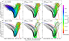 |
Fig. 7. BPT diagrams used to classify our samples into different galaxy types (Kewley et al. 2006b). The red line separates active galactic nuclei (AGN) and composite galaxies (COMP) (Kewley et al. 2001). AGNs and low ionisation narrow emission line regions (LINER) are separated by the green line (Schawinski et al. 2007) and the blue dashed lines separate star forming (SF) and COMP (Kewley et al. 2006b). We present the CS in the upper left panel and the NBCS in the lower left panel. In the upper middle (resp. right) panel, we show the blueshifted (resp. redshifted) peaks of DP galaxies with a S/N > 3 in the four emission line fluxes needed for the BPT diagram. In the lower middle and right panels, we display those emission line components of the DPS with three of the requested emission lines with S/N > 3 and the fourth S/N < 3. To classify them, we display arrows to indicate the limits derived by the uncertainties of weak emission lines. In all six panels, we apply the same colour-coding indicating the specific star formation rate (SSFR) computed by Salim et al. (2016). We display in all panels the same contour lines corresponding to the density of the CS. The corresponding classifications are presented in Table 4. |
We classified the two emission line components according to their position on the BPT diagram if all four needed emission lines have a S/N > 3. In the case where we only have three emission lines with a S/N > 3, we computed the upper or lower limits derived from the uncertainties of the undetected emission line. If the constraints of these emission line ratios are unambiguous, we could classify them. Since the COMP region in the first BPT diagram borders the AGN and the SF regions, it was not possible to classify galaxies as COMP unambiguously using the flux limits. In Fig. 7, we show the classification of the single lines of the CS, the NBCS and each emission line component of the DPS. We also show with arrows upper or lower limits of these DP galaxies, which only have three significant emission line components. In all BPT diagrams, we colour-code the specific star formation ratio computed by Brinchmann et al. (2004).
The classification of the first BPT diagram type using all four emission lines with a S/N > 3 was used first. This classified about 67% of the bluer and the redder peaks. Galaxies with only three significant emission lines in the first diagram type were classified using the upper or lower limits, which comprises about 16% of the blue and the redshifted peaks. With the second and the third types of BPT diagrams, we only classified 0.4% of the two peak components with all four emission lines having a S/N > 3. Numerous peak components could not be classified using the upper or lower limits in the second or the third diagram types. This is because if the [NII]6585 line is weak, the [SII]6718, [SII]6733 or the [OI]6302 lines are usually not detected. To directly compare the DPS with the CS and the NBCS, we also performed the same BPT classification as for the CS and NBCS but with the non-parametric emission line fit performed by Chilingarian et al. (2017). This classification shows 80–90% agreement with those DP, classified the same way in each component (e.g. double SF). We present the final BPT classification in Table 4 for all the three samples, namely DPS, CS and NBCS.
We classified 88 945 (99.5%) galaxies of the CS, 5032 (98.1%) of the NBCS and 5423 (95.4%) galaxies from the DPS with an individual classification and 4818 (85.1%) using the non-parametric fit. The majority of the CS galaxies are SF 92%, while only a small amount is classified as COMP (5%) and only a few galaxies, about 2% (resp. 1%), are classified as AGN (resp. LINER). This is not surprising since we know from Fig. 5 that the CS comprises many small galaxies. This classification is different for the NBCS: the majority (55%) is still classified as SF but we find around 24% to be classified as COMP, and 13% (resp. 6%) as AGN (resp. LINER). In comparison, we classified 45% of the DPS as SF using the non-parametric emission line fit. About 38% of the DPS are classified as COMP showing that we find less SF and more COMP galaxies in comparison to the NBCS. We find a similar AGN fraction of about 11% (13%). We find twice the fraction of galaxies classified as LINER in the NBCS (6%) in comparison to the DPS (3%).
By classifying each emission line component of the DPS, we find 29% (resp. 17%) to be classified as SF (resp. COMP) in both emission line components. We also find 14% of the DPS galaxies with one component to be classified as SF and the other one as COMP. According to Kewley et al. (2006b), COMP galaxies are a combination of a SF and a AGN nucleus or a SF and LINER emission. Counting all galaxies which have at least one emission line component classified as COMP, we find 45%. This is an excess of about a factor 2 in the DPS in comparison with the NBCS (24%). Counting only all galaxies classified as ‘double SF’ or ‘SF and uncertain’ in the second peak, we find 39% of the DPS, which is significant less in comparison with the NBCS (55%).
Many works published in the recent years were focused on double-peak emission line AGNs with the motivation to find dual AGNs (see Sect. 1). Here, we do not observe the DPS to be dominated by this type of galaxies. We observe about 7% double AGN or LINER classification and 3% with one AGN or LINER and one uncertain. We furthermore find 6% to show a mixed classification with one AGN or LINER component. In comparison with the NBCS, which comprises about 19% to be classified as AGN or LINER, we find less AGN and LINER in the DPS. We recall that QSO and Seyfert1 galaxies have been excluded from the RCSED (Schneider et al. 2010; Chilingarian et al. 2017), which can explain the lack of galaxies classified as AGN in this catalogue (see also Sect. 2.4). Smith et al. (2010) concentrated on DP QSO and find 148 DP galaxies, which are not treated in this work (see Sect. 2.4).
3.2. Morphological classification
We identified the morphological types of our galaxy samples using Domínguez Sánchez et al. (2018), which is a machine-learning-based algorithm to identify different types of galaxy morphologies. Different neuronal networks have been trained with SDSS gri colour composite images on various criteria to determine their morphology. To classify our samples, we used the following variables to define the probability of an observed feature: Pdisc for disc features, PS0 for S0 galaxies, Pedge-on for edge-on orientation, Pmerger for visual merger and Pbar for a bar structure. The T-type relates each galaxy to a type classification on the Hubble sequence. To classify spiral galaxies according to their inclination, we calculated the inclination angle i as:
 (5)
(5)
where b/a is the r-band minor-to-major axial ratio estimated by Meert et al. (2015), while q0 is the intrinsic axial ratio of galaxies observed edge-on and is set to q0 = 0.2. The inclination for galaxies with b/a < 0.2 is set to 90° (Catinella et al. 2012; Aquino-Ortíz et al. 2018). Relying on Domínguez Sánchez et al. (2018) and through inspection of the selected SDSS images, we find the following arguments:
– Late-type galaxies (LTG), which are disc dominated2, are selected by T-type > 0 and Pdisc > 0.5.
– Face-on are identified as LTG with an inclination angle smaller than 30°. To further decrease the false-positive detection rate, we demand Pedge-on < 0.1.
– Edge-on and strongly inclined galaxies are selected as LTGs with an inclination angle larger than 70° and Pedge-on > 0.4.
– Barred galaxies are LTGs with Pbar > 0.9 and Pedge-on < 0.5
– S0 galaxies are selected by a T-type ≤ 0, PS0 > 0.6, Pdisc < 0.3 and Pedge-on < 0.4
– Elliptical are characterised by a T-type ≤ 0 and PS0 < 0.3
– Merger galaxies are selected by using Pmerger > 0.9. This high threshold provides a sub-sample of merger with high purity enabling to test if visible merging processes are at the origin of DP galaxies.
To compare our galaxy samples with respect to their morphological classification, we did not apply any subjective correction to the selection. We computed the fraction of all classified types for the DPS, the CS and the NBCS in Table 5. Figure 8 displays the redshift distribution for the different morphological types of the DPS and the NBCS. We observe merger and S0 galaxies to be more distant in comparison to LTG and elliptical galaxies. This can be the result of a classification bias as discussed in the training sample (Willett et al. 2013) used for the classification in Domínguez Sánchez et al. (2018). We thus might misclassified LTG as S0 galaxies because of their distance. In Fig. D.2, we illustrate the morphological types, by showing 20 randomly selected galaxies for each type (except for the face-on LTGs, for which we show all ten cases).
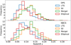 |
Fig. 8. Redshift distribution of the DPS for LTG, S0, merger, and elliptical galaxies. We unified the histogram surface of all four samples to 1. |
Morphological classification of the DPS, the CS and the NBCS.
In Table 5, we find that the majority of the CS galaxies are not classified (62%). This is due to a classification bias against small and weak galaxies (Domínguez Sánchez et al. 2018). The numbers of not classified galaxies in the DPS and the NBCS are comparable (35% and 38%). By comparing the morphological classification of the DPS and the NBCS, we find two noticeable effects. On the one hand, LTG are less numerous in the DPS (16%) than in the NBCS (30%). On the other hand, more S0 galaxies are present in the DP (36%) than in the NBCS (20%). These results are visualised in Fig. 9.
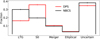 |
Fig. 9. Fraction of different morphological types for the DPs and the NBCS. The error-bars represent the binomial errors. |
We find in both samples a similar merger rate of ∼10%. This observation is a priori contradictory to the idea of a DP structure due to a major galaxy merger but does not exclude the possibility that DP galaxies might be minor mergers, post-mergers or hidden merger. Furthermore, the same merger rate (10%) was found in a recent double-peak sample in the Large Sky Area Multi-object fibre Spectroscopic Telescope survey (Wang et al. 2019b). As a cross-check, we performed a visual inspection of the first 1000 galaxies in the DPS and the NBCS. We find a merger rate of 11.4% (resp. 11.7%) for the DPS (resp. NBCS), which is close to the merger rate we extracted from Domínguez Sánchez et al. (2018). By lowering the selection threshold for mergers (e.g. Pmerger > 0.8 or Pmerger > 0.7), we do not detect different merger rates in the DPS and the NBCS, but higher rates of misclassification.
We also classified LTGs in face-on (0.2%), edge-on (1.0%), and bar (1.9%) galaxies. We chose strict selection criteria to avoid false-positive classification for face-on and edge-on galaxies. These galaxy types are interesting since edge-on galaxies may exhibit a double horn due to a rotating disc, while face-on galaxies should not exhibit rotation in form of a DP. We do not observe any excess of edge-on galaxies in comparison to the NBCS (2.2%). In Sects. 4.3.3 and 4.3.4, we discuss arguments using the inclination.
We also provide cross-matches between the morphological types and the BPT classifications in Tables D.1 and D.2 and provide a statistical significance test in Appendix A.
4. Analysis
4.1. General characteristics
To describe the characteristics of the DPS and compare them with the NBCS and the CS, we show in Fig. 10 the distribution of six parameters: the Galactic extinction and k-corrected absolute magnitude of the r-band Mr, SSFR = SFR/M⊙, the luminosities of the [OIII]λ5008 and Hαλ6565 emission lines, stellar population ages, and stellar metallicities.
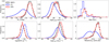 |
Fig. 10. Different parameters distributions of the DPS (red), the CS (blue) and the NBCS (black). The surfaces of all histograms are normalised to unity. In the upper left panel, we compute the absolute AB magnitude in the r-band with Galactic dust and K-corrections estimated by Chilingarian et al. (2017). The lower left panel shows the specific star formation ratio (SSFR) computed by Brinchmann et al. (2004). The middle upper (resp. lower) panel presents the absolute luminosity of the [OIII]λ5008 (resp. Hαλ6565) emission line. The absolute luminosity is calculated using the flux of the non-parametric emission line fit provided by Chilingarian et al. (2017). The right upper panel computes the age assumed by a single stellar population fit by Chilingarian et al. (2017). The right lower panel shows the stellar metallicity computed by Chilingarian et al. (2017). |
In every distribution, the CS differs from the DPS whereas the NBCS shows good agreement with the DPS, except for the Hαλ6565 luminosity. We discuss in Sect. 4.2 that this is related to a significant difference in the star formation activity. As discussed in Sects. 2.2.3 and 2.3, the CS follows a different stellar mass-redshift distribution in comparison to the DPS and the NBCS. On average, the CS shows smaller Mr, higher SSFR and smaller absolute luminosities in the [OIII]λ5008 and Hαλ6565 line than the DPS and the NBCS. This different behaviour observed for galaxies of the CS is mainly due to a sensitivity bias: low-mass galaxies pass the signal-to-noise ratio cut on the emission lines while the DPS and NBCS are large-mass galaxies (see Sect. 2.3).
The differences in the DPS and NBCS Hαλ6565 luminosities are small: LHα(DPS) = 41.16 ± 0.36 and LHα(NBCS) = 40.96 ± 0.42 (mean and standard deviation). However, using a the non-parametric Kolmogorov-Smirnov test to distinguish weather the two distributions are the same or not, we find a k-statistic of 0.235 marking the maximal distance of the cumulative distribution function and a p-value of 5 × 10−130, strongly indicating that these two distributions are different.
We checked the extinction based on the Balmer decrement and found that DPS galaxies have slightly more extinction (0.25 mag higher in V) than the NBCS galaxies, while this effect is stronger for LTG and S0 galaxies (see Fig. C.1).
To approximate stellar ages, we used the spectral continuum fit performed with a SSP (Chilingarian et al. 2017). Due to the cut on the stellar masses (see Figs. 5 and 6), the CS is dominated by young stellar populations with an SSP-based age between 1 and 2 Gyr in 52% of the galaxies. Nearly all (97%) of these young galaxies are classified as SF (see Sect. 3.1). The NBCS and DPS show comparable distributions but with on average an older stellar population than for the CS. The majority (74% and 71% respectively) of the two samples is younger than 5 Gyr, while 47% (DPS) and 66% (NBCS) of these young galaxies are SF galaxies. We also find that 29% (resp. 23%) of the young DP galaxies (resp. NBCS) are classified as COMP. Last, we find 15% of the DPS to be classified with one peak as COMP and the second one as SF. As discussed in Sect. 3.1, we find an excess of the percentage of SF galaxies in the NBCS and CS whereas we do not find such a high excess in the DPS. We also show the stellar metallicity, computed by Chilingarian et al. (2017), and find that the DPS and the NBCS follow the same distribution, whereas the CS shows a different distribution with lower metallicity values. This is expected due to the difference in stellar mass of the different samples (Tremonti et al. 2004).
While we find many differences between the DPS and the CS, the NBCS and DPS distributions are similar. The NBCS is therefore well suited to identify the peculiarities of the DPS.
4.2. Star formation vs. AGN excitation
SF is important to characterise the state of evolution of a galaxy and to estimate its growth rate. In Sects. 3.1 and 4.1, we find that the majority of the DPS, CS and NBCS show SF activity. At the same time, we find AGN activities (or galaxies classified as COMP) in the NBCS and the DPS. To further analyse and compare our samples, we used diagnostic colour-colour diagrams, specific star formation rate (SSFR) and stellar mass diagrams and compare the SFR of the 3″ SDSS fibre and of the total galaxy. According to Salim et al. (2007), the SFR of AGN computed by Brinchmann et al. (2004) can be overestimated. We therefore used the NUV-band to compute the SFR and found a good agreement to the SFR measured by Brinchmann et al. (2004) for our galaxies classified as AGN. We discuss AGN excitation of galaxies classified as composite galaxies and cross-match our catalogues with radio observations.
In Fig. 11, the g − r vs. NUV − r colour-colour diagram shows a single sequence with the star-forming blue cloud and the red sequence, characterised by quenched star formation (Strateva et al. 2001; Hogg et al. 2002; Ellis et al. 2005), separated by a critical value of NUV − r = 4.75. The blue cloud (resp. red sequence) is approximately represented by blue (resp. red) contours for LTGs (resp. elliptical galaxies) from the RCSED (compare with Chilingarian & Zolotukhin 2012). We find the DPS to be situated in the upper region of the blue cloud and only some outliers in the red sequence. We do not find significant effects for the different subsets classified in Sect. 3. We can thus conclude that the DPS and the NBCS are not quenched and are mainly associated with the main star forming sequence. The distribution of the DPS is more concentrated in the range centred at NUV − r ∼ 3.5 than the NBCS (NUV − r ∼ 3.0), which is centred in the blue cloud. This shift towards redder colours can be explained by considering shorter time scales τ of an exponential declining star formation history, as shown in Chilingarian & Zolotukhin (2012).
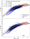 |
Fig. 11. Colour-colour relation between g − r and NUV − r. We present LTG and elliptical galaxies selected from the RCSED catalogue using Domínguez Sánchez et al. (2018) as blue and red contours and show the DPS (resp. NBCS) as black dots in the top panel (resp. lower panel). We display the best-fitting polynomial surface equation of constant absolute z-band magnitudes with coloured lines (Chilingarian & Zolotukhin 2012). |
However, this is not the case for the DPS as their mean τ is slightly larger than for the NBCS. We argue that these redder colours are most probably to the mean extinction estimated to AV = 0.25, as displayed in the last column of Fig. C.1.
We can notice some galaxies in the DPS situated below the two sequences in Fig. 11. This area is associated with post starburst galaxies which underwent a recent massive starburst that is now quenched (Chilingarian & Zolotukhin 2012). Such galaxies can be also situated in the surface, as they can be biased when a strong Hαλ6565 line contributes to the r-band magnitude, shifting the position of the galaxies into the plane. We find that this is not the case for DP galaxies, nor the NBCS. To confirm this, we studied the colour-colour diagram with colours g − z and NUV−z, where this off-plane shift disappears.
In Fig. 12, we show the SSFR, taken from Brinchmann et al. (2004), as a function of the stellar mass, computed by Kauffmann et al. (2003). With this diagnostic diagram, Schiminovich et al. (2007) distinguished between the blue and the red sequence in terms of SSFR and stellar mass. Salim (2014) associated intermediate NUV−r colours known as the “green valley” with intermediate star formation of −11.8 < log(SSFR/M⊙) < −10.8 suggesting that these galaxies might be in transition. In Fig. 12, we show the distribution of LTGs and elliptical galaxies selected from the RCSED as reference. We display the 50%, 68% and 95% contour levels of different morphological types of the DPS and the NBCS. We find, depending on the morphological type, between 6% and 26% (resp. 8% and 43%) of the DPS (resp. NBCS) showing intermediate star formation. We only find a significant difference between the DPS and the NBCS for elliptical galaxies: only 26% of the elliptical DP galaxies show intermediate star formation whereas 43% of the elliptical galaxies of the NBCS are situated in this region. We find indeed very similar distributions for all different morphological types of the DPS and thus conclude that SF and the stellar mass are not depending on the morphological type.
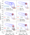 |
Fig. 12. SSFR as a function of stellar mass. The top left panel presents LTG and elliptical galaxies selected from the RCSED catalogue using Domínguez Sánchez et al. (2018) as blue and brown contours. These contours are also shown as a reminder in the other panels. We show contour lines indicating the 50%, 68% and 95% level for different morphological subsamples of the DPS (red) and the NBCS (black). We indicate with blue dashed lines the region of intermediate star formation (−11.8 < log(SSFR/M⊙) < −10.8) (Salim 2014) and display the percentage of the morphological types situated in this zone. |
To discuss the SF in a quantitative way, we used SFRs estimated by Brinchmann et al. (2004) for the entire galaxies (SFRtotal) and for the 3″ SDSS fibre (SFRfibre). Since the proportion of a galaxy covered by the 3″ fibre depends on its redshift, we divided the DPS and the NBCS into three groups of redshift ranges: z < 0.075, 0.075 < z < 0.125, and 0.125 < z. In order to discuss the SF activities in detail, we especially examined the sub-samples classified as double SF and AGN, using the BPT classification performed in Sect. 3.1.
Hence, we present the comparison between the DPS and the NBCS with the difference between total and 3″ absolute r-band magnitude, the ratio of the Petrosian radii of 90% and 50%, the SFRfibre and the ratio ℛ = SFRfibre/SFRtotal. We show these observables for the three redshift groups for galaxies of the DPS classified as double-SF (resp. double-AGN) and SF (resp. AGN) galaxies of the NBCS in Fig. 13 (resp. Fig. 14). For double-SF galaxies of the DPS, we find an excess of luminosity in the centre and a higher SFRfibre in comparison to SF galaxies of the NBCS. This excess is most prominent for galaxies with a redshift z < 0.125, corresponding to maximal fibre diameter of 7.6 kpc. With respect to SFRtotal, we find a clear enhanced-central-SF activity for double-SF galaxies of the DPS in comparison to SF galaxies of the NBCS. We find a median SFR ratio for double-SF galaxies of the DPS with a redshift z < 0.075 of  . For SF galaxies of the NBCS in the same redshift range we find
  . We find similar values for galaxies with a redshift 0.075 < z < 0.125, whereas this effect is slightly weaker for galaxies with z > 0.125. This is due to the fact that for more distant galaxies the 3″ fibre covers the majority of the surface of the galaxies, therefore SFRfibre tends to SFRtotal. We summarise the median SFR ratios and the 68-percentile for different galaxy types in Table 6. We also find an enhanced-central-SF for LTGs, S0 galaxies and galaxies classified as double COMP at lower redshift.
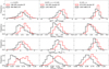 |
Fig. 13. Distribution of different observables within the 3″ SDSS fibre. We show in three columns three different ranges of redshift. We present galaxies of the DPS which are classified as double SF in red and galaxies classified as SF of the NBCS in black (see Sect. 3.1) In the top row we show the difference in absolute r-band magnitude of the total galaxy and the 3″ SDSS fibre. The colours are Galactic dust- and k-corrected (Chilingarian et al. 2017). In the second row we present the ratio of the radii comprising 90% and 50% of the Petrosian luminosity (Petrosian 1976) approximating the central brightness in comparison to the total galaxy. We show the star formation ratio of the 3″ SDSS fibre SFRfibre in the third row and the ratio between fibre and total star formation (SFRfibre/SFRtotal ) in the bottom row (Brinchmann et al. 2004). |
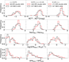 |
Fig. 14. Comparison of absolute r-band magnitude, Petrosian radii and SFRfibre and SFRtotal as in Fig. 13 but with DP galaxies classified as AGN in both peak components (red) and galaxies of the NBCS classified as AGN (black). |
Median ratios of fibre and total SFR.
Double-AGN of the DPS follow the same SFRfibre and SFRtotal distributions as the AGNs of the NBCS and no enhancement of central SF activity or central luminosity is observed as shown in Fig. 14.
With the BPT classification in Sect. 3.1, we find less SF but more COMP galaxies in the DPS in comparison to the NBCS. Since COMP galaxies are understood to be a mixture of SF and AGN (Kewley et al. 2006b), we quantified the AGN excitation using the [OII]λ3728 and the [NeV]λ3426 emission lines.
(1) The ratio [OII]λ3728/[OIII]λ5008 can be used to distinguish between a pure AGN and SF. From photo-ionisation models, a value between 0.1 and 0.3 is used for a pure AGN (Tammour et al. 2015), while above a value of 0.3, the [OII]λ3728 flux is thought to be produced in SF sites (Osterbrock & Ferland 2006). Using the non-parametric emission line fit from Chilingarian et al. (2017), we find a mean ratio of [OII]/[OIII] = 0.23 ± 0.14 for galaxies classified as double AGN. For double SF (resp. COMP) galaxies, we find [OII]/[OIII] = 1.57 ± 0.56 (resp. 1.14 ± 0.54). This indicates that galaxies which are classified as COMP are dominated by SF. This effect can also be biased by extinction in dusty galaxy centres and must therefore be considered with caution.
(2) We then discuss galaxies with AGN activity based on the detection of the high-ionisation [NeV]λ3426 emission line (Gilli et al. 2010; Vergani et al. 2018). Due to redshift, the [NeV]λ3426 line is only detected in SDSS spectra from z > 0.2. We inspected spectra of the DPS galaxies classified as double-SF, -COMP and -AGN for [NeV]λ3426 detection. We find no galaxies classified as double-SF contrary to 62% of the galaxies classified as double-AGN having a detectable [NeV]λ3426 line. Only 4% of the z > 0.2 galaxies classified as double COMP show this line which supports the evidence that these are SF galaxies.
To discuss further aspects on the connection between AGN excitation and SF in our galaxy samples, we cross-matched the DPS and the NBCS with surveys of radio observations. It has been known for a long time that non-thermal radio emission is linearly correlated to the far-infrared flux (Helou et al. 1985; Condon 1992; Sanders & Mirabel 1996), while IR luminosity is a good SF tracer (e.g. Kewley et al. 2002). More recently, the radio luminosity at 150 MHz has been considered as a potential tracer of SF (Calistro Rivera et al. 2017; Wang et al. 2019a). We useed FIRST at 1.4 GHz (White et al. 1997) and the first data release of the LOFAR Two-metre Sky Survey (LoTSS; Shimwell et al. 2019) at about 150 MHz. Roughly 20% (1154) of the DPS are detected with FIRST, but only 8% (395) of the NBCS. In the observed field of the LoTSS DR1 we find a detection rate of 73% (237) for the DPS and 56% (191) for the NBCS. We find a significant excess of radio sources at 1.4 GHz and a higher detection rate at 150 MHz for the DPS in comparison to the NBCS. We will further explore the radio properties of these galaxies in Maschmann et al. (in prep.).
4.3. Kinematic properties of the double-peak galaxies
4.3.1. Velocity distributions
To explore the gas and star kinematic properties of our samples, we present basic velocity estimates to assess possible differences between the DPS, the CS and the NBCS. In Fig. 15, we show the stellar velocity dispersion σ* and the gas velocity dispersion σgas.
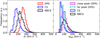 |
Fig. 15. Velocity dispersion distributions for the CS (blue), the NBCS (black) and the DPS (red, purple and orange). The left panel displays the stellar velocity dispersion σ* computed from Chilingarian et al. (2017). The second panel shows the gas velocity dispersion σgas. We compute the Gaussian emission line dispersion for the CS and the NBCS from (Chilingarian et al. 2017). For the DPS, we display the σ1, 2 of the emission line components, which is closer to the galaxy stellar velocity in units of σ1, 2 in magenta and the component which is more offset in cyan. For better comparisons, we unify the surface of the histograms of the left (resp. right) panel to 150 (resp. 100). |
The stellar velocity dispersion was computed in Chilingarian et al. (2017), fitted with a SSP and an EXP-SFH (see Sect. 2). We computed the  for both fit functions and selected the resulting stellar velocity dispersion from the best fitting function.
To compute the gas velocity dispersion for the CS and the NBCS, we used the velocity dispersion measured for all Balmer and forbidden lines in Chilingarian et al. (2017) and show the one of the strongest line. For double-peak emission lines, we used the stacked emission line spectra (see Sect. 2.2.2) and compute the σclose which corresponds to the DP component closer to the galaxy velocity in units of σ and σfar to the component which is more offset.
As shown in Fig. 15, we observe a higher σ* for the DPS in comparison with the CS and the NBCS. The gas velocity dispersion σgas indicates higher velocities for the NBCS and the DPS in comparison to the CS. This is expected from the Tully-Fisher relation, since these two samples comprise more massive galaxies (Tully & Fisher 1977). For the DPS, we find the velocity dispersions, measured for the close peak, to be compatible with the gas velocity dispersions of the NBCS. For the far peak of the DPS, the velocity dispersions are systematically smaller.
4.3.2. Single Gaussian approximation for DP
To discuss possible mechanisms behind double-peak emission lines, we need to compare the gas kinematics of the DPS and the NBCS. In order to do so we used the single Gaussian approximation of the double-peak emission lines, as computed in Sect. 2.2.2.
A single Gaussian fit to the complex line shape of DP galaxies provides a measure of the velocity dispersion assuming the DP originates from one system. In Fig. 16 we show one stacked emission line, the double Gaussian fit and the single Gaussian fit performed in Sect. 2.2.2.
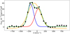 |
Fig. 16. Single Gaussian approximation. We compute the two Gaussian functions resulting from the double Gaussian fit procedure to the stacked emission line in Sect. 2.2. The blueshifted component is represented by a blue and the redshifted by a red line. In orange, we show the best fit of a single Gaussian function. |
In Fig. 17, we show σ* on the x-axis and on the y-axis σgas for the NBCS and σsingle for the DPS. We display the median and the 68% percentile of σgas and σsingle with a binning according to σ*. The emission line parameters σ1, 2 and ΔvDP of the DPS are restricted by a lower limit, defined with the spectral resolution (see Sect. 2.2.2). We thus find a lower threshold of 114 km s−1. Similarly, for the NBCS, we find a minimal σgas of 43 km s−1.
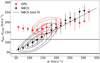 |
Fig. 17. Comparison of the stellar velocity distribution σ* computed by Chilingarian et al. (2017) with the gas velocity distribution σgas for the NBCS and the velocity distribution of the single Gaussian approximation σsingle for the DPS. We show in red (resp. black) points the median and the 68% quantile for a binning according to σ* of the DPS (resp. NBCS). For the DPS, the limitations in σ1, 2 and ΔvDP of the double Gaussian fit are restricted by the spectral resolution (see Sect. 2.2.2), leading to a restriction of a minimal σsingle, indicated with a red line. We also show the minimal σgas for the NBCS as a black line and the best fit of a linear function as a black dashed line. |
By comparing σgas with σ* of the NBCS, we find a linear relation described by σgas = 0.71 σ* + 23.8 km s−1 (black dashed line in Fig. 17). This relation might be valid for σsingle and σ* of the DPS for higher velocities (σ* > 150 km s−1). In this regime, we can assume a linear relation for the DPS but we still find a shift towards higher velocities in comparison to σgas of the NBCS. This suggests that the gas components of DP galaxies show higher velocities in comparison to σ*, or that one part of the ionised gas is strongly perturbed or has an external origin.
4.3.3. Inclination
A double-peak emission line shape can of course also originate from a rotating disc. This has been discussed in detail in Elitzur et al. (2012) and shown in simulation in Kohandel et al. (2019). In order to test this specific scenario, we used a single Gaussian approximation of the double-peak emission lines (see Sect. 4.3.2) which, in the case of a rotating disc, would be an approximation for the gas velocity dispersion. We assumed here that the rotation disc is the main disc of the galaxy, and study the correlation of the velocity dispersion with the inclination angle i defined with the photometric analysis. Hence, we calculated the inclination angle following Eq. (5) using the minor-to-major axis measured by Meert et al. (2015) which provides reasonable results for spiral and S0 galaxies if the disc component exhibits good fit results (see Meert et al. 2015, for more details on fit results). As a cross-check for the measured inclination, we followed Yip et al. (2010) and find a dependency between the inclination angle and the Balmer decrement Hα6565/Hβ4863 used to calculate the inner galactic extinction. This trend is comparable to the one observed for the NBCS, but, as mentioned above, the extinction is slightly larger (0.25 mag) for DPS than for NBCS.
The area covered by the 3″ SDSS fibre depends on the redshift. The measured gas velocity dispersion of a rotating disc depends on the area integrated by the spectroscopic observations. We thus defined three redshift groups as in Sect. 4.2 for this analysis: z < 0.075, 0.075 < z < 0.125, and 0.125 < z. In Fig. 18, we present the estimated inclination angle i as a function of various gas velocity measurements for the DPS and the NBCS. The NBCS is represented by the gas velocity dispersion σgas (see Sect. 4.3.1). For the DPS, we display σsingle from the single Gaussian approximation (Sect. 4.3.2), ΔvDP from the stacking procedure (Sect. 2.2.2) and σclose and σfar as described in Sect. 4.3.1. For galaxies with a redshift z > 0.075, we see a clear correlation in the NBCS between σgas and the galaxy inclination i. This correlation between σgas and i can be explained by a rotating disc. In contrast, we do not find any dependencies between the displayed velocities of the DPS and i in any redshift range. The absence of such a correlation for the DPS disfavours the rotating (main-) disc scenario.
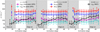 |
Fig. 18. Influence of the inclination on the velocity dispersion. We show different velocity dispersion distributions as a function of the galaxy inclination for different groups of redshift. We only show LTG and S0 galaxies for which we can compute the inclination using Meert et al. (2015). For the DPS, we show ΔV with red dots, σsingle of the single Gaussian approximation in blue (see Sect. 4.3.2) and in magenta (resp. cyan) the σ of the emission line component which is closer (resp. offset) to the stellar velocity in units of σ. We show the σgas for the NBCS with black dots. All data points represent the medians in the inclination intervals and the error bars the 16th to 84th percentiles. |
4.3.4. Tully-Fisher and Faber-Jackson relations
The velocities measured in galaxies are tightly correlated to their size. This relation was first discovered by Faber & Jackson (1976) for the stellar velocity dispersion and the absolute magnitude of elliptical galaxies (FJR). They concluded that the luminosity L of a galaxy is consistent with the relation  . In parallel, a good relation between the full-width at 20% of the maximum of the HI profile, corrected to the inclination of the galaxy, and the galaxy size was found by Tully & Fisher (1977) for spiral galaxies. This Tully-Fisher relation (TFR) is usually understood as the self-regulation of star formation in the disc (e.g. Silk 1997).
The parameters of these relations have been later measured with higher accuracy. Here, we used for the FJR: log(σ*/km s−1) = −0.90 ± 0.12 + (0.29 ± 0.02) log10(M*/M⊙), measured by Gallazzi et al. (2006). For the TFR, we use: log10(vrot/km s−1) = − 0.69 + (0.27 ± 0.01) log10(M*/M⊙), measured by Avila-Reese et al. (2008), where vrot is the rotation velocity, calculated as in Catinella et al. (2005) and Aquino-Ortíz et al. (2018): vrot = W/[2 sin i], where i is the inclination angle (see Eq. (5)) and W the difference between the 10th and the 90th percentile of the velocity measurements. Since we do not have spatially resolved information on galaxy kinematics, we approximated from a Gaussian shaped emission lines the 10th and the 90th percentile as W = 2.56σ (this is close to the full-widths half maximum of a Gaussian at 2.36σ). We calculated vrot for the TFR using σgas for the CS and the NBCS (see Sect. 4.3.1) and σsingle, σclose and σfar for the DPS (see Sects. 4.3.1 and 4.3.2). We take the stellar mass log(M*/M⊙) measured by Kauffmann et al. (2003) for the TFR and FJR. In the case where we display only one of the DP (the close or the far peak), we approximated the fraction of the stellar mass for each peak as log(f1, 2 M*/M⊙). We assumed f1, 2, the mass fraction of each peak, to be the same fraction as the total emission line flux of the stacked lines. This is a rough approximation but would be our best guess to assume each peak corresponds to one component of a hidden merger.
In Fig. 19 (resp. 20), we present the TFR for LTG (resp. S0) of the DPS, the CS and the NBCS. We find good agreement for LTG of the CS and the NBCS with the parameters for the TFR found by Avila-Reese et al. (2008). We find that, for the LTGs of the DPS, the rotation velocity calculated with σsingle does not follow the TFR. We measure vrot to be higher than expected for the measured masses. We find a good agreement using σclose whereas rotation velocities calculated with σfar are shifted towards lower velocities. For S0 galaxies, we observe the same velocity shifts as shown in Fig. 20. S0s and LTGs have a similar behaviour: σsingle is offset with respect to the NBCS distribution considering the two peaks as individual galaxies following this distribution. In both TFRs, we find some outliers with extreme vrot values. By individual inspection, we find these velocities to be the result of a small inclination and/or very broad peak component.
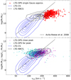 |
Fig. 19. Tully-Fisher relation (TFR) for LTGs. We compute the rotational gas velocity vrot for the NBCS and CS (black and blue contour lines) using the gas velocity dispersion σgas (see Sect. 4.3.1). For the DPS, we use the σsingle of the single Gaussian approximation in the top panel. In the second panel, we show the TFR for the close and far peak-components of the DPS (see Sect. 4.3.1). The stellar masses are computed by Kauffmann et al. (2003). We show the best fit computed by Avila-Reese et al. (2008) as a dashed line. |
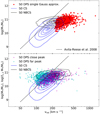 |
Fig. 20. Same as Fig. 19, but for S0 galaxies. The dashed line corresponds to the best fit of Avila-Reese et al. (2008). |
In Fig. 21, we show the FJR (M* vs. σ*) for elliptical and S0 galaxies. As a reference, we used the best fit from Gallazzi et al. (2006) as a dashed line. We find good agreement for elliptical galaxies of the DPS, CS and the NBCS. For S0 galaxies, we find in the NBCS and the CS systematically lower σ*, whereas the DPS shows velocities agreeing with those of elliptical galaxies with the same stellar mass. This is in agreement with the result discussed in Fig. 15 that the stellar velocity dispersion is larger for the DP galaxies, supporting again a large system composed of the superposition of two systems.
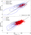 |
Fig. 21. Faber-Jackson relation for elliptical and S0 galaxies using the stellar velocity dispersion taken from Chilingarian et al. (2017) on the x-axis and the stellar masses computed by Kauffmann et al. (2003) on the y-axis. We show the best fit computed by Gallazzi et al. (2006) in dashed lines. |
4.4. Morphology and galaxy environment
We studied the environment of the DP galaxies with the galaxy group catalogue provided by Yang et al. (2007)3 and Saulder et al. (2016). Yang et al. (2007) is a halo-based group finder algorithm, determining the group masses and identifying each member of groups using the redshift. About 90% of the DPS and the NBCS are covered by this catalogue. Saulder et al. (2016) calibrated a group finder algorithm with simulation data providing a higher sensitivity to different kinds of galaxy groups up to a redshift of z < 0.11 (47% of the DPS and NBCS). In this redshift range, they cover 97% (resp. 98%) of the DPS (resp. NBCS).
We used galaxy groups sizes as discussed in Blanton & Moustakas (2009): a poor group holds 2 to 4 members, a rich group 5 to 9 and a cluster more than 10. With Yang et al. (2007), we find 64% (resp. 66%) of the DPS (resp. NBCS) to be isolated, 19% (resp. 17%) in poor groups, 3% (resp. 4%) in rich groups and 4% (resp. 4%) in clusters. To compare this result with Saulder et al. (2016), we looked at the fraction for galaxies with redshift z < 0.11 and find similar fractions as above. Using Saulder et al. (2016), we find 45% (resp. 45%) of the DPS (resp. NBCS) to be isolated, 34% (resp. 33%) in poor groups, 11% (resp. 12%) in rich groups and 9% (resp. 12%) in clusters. We detect fewer isolated galaxies in comparison to Yang et al. (2007), which is due to the higher sensitivity of group identification.
In Table D.3, we present the fractions of the environmental classification for the morphological types (see Sect. 3.2). Analysing group properties such as number of group members, distance to the closest neighbour or the velocity dispersion of a galaxy group, we only find a difference between the DPS and the NBCS for elliptical galaxies (Saulder et al. 2016). In the DPS (resp. NBCS), we find 23% (resp. 41%) of the elliptical galaxies to be situated in a dense environment (rich groups or clusters), whereas 72% (resp. 58%) are situated in less dense environments (isolated galaxies or poor groups).
S0 galaxies are usually observed more abundant in clusters than in the field (Dressler 1980), but this is not the case here. In the DPS and the NBCS, we find about 80% of the S0 galaxies to be situated in less dense environments. We do not find any differences in the fraction of isolated S0 galaxies selected in the DPS and the NBCS, but we clearly see that most of the selected S0 galaxies are isolated. Even though we find an excess of S0 galaxies and a lack of LTGs in the DPS in comparison to the NBCS (see Sect. 3.2), we do not find any connection between the galaxy environment and the morphological type.
Dressler et al. (1997) first observed an increase of S0 galaxies over elliptical fraction in groups from z ∼ 0.5 till today, while the spiral fraction before z ∼ 0.5 corresponds to the S0 fraction observed today. This supports the view that spirals evolve into S0 galaxies due to their environment (Fasano et al. 2000). This has been supported by subsequent observational works (e.g. Wilman et al. 2009). However, this is not the case here as 70% of the DP-S0 galaxies are isolated according to Yang et al. (2007), (or 50% for z < 0.11 according to Saulder et al. 2016), and the behaviour of S0 and LTG are not significantly different in the DPS in terms of excitation mechanisms and dynamics. This apparently contradicts the work of Gao et al. (2018), based on photometric decomposition, who found that the bulges of spirals and S0s are intrinsically different and thus spirals are probably not the progenitors of S0s.
4.5. Non-parametric morphological diagnostics
To further investigate the properties of the different morphological galaxy types, we computed photometric diagnostics for the DPS and NBCS. We used the python package STATMORPH4, which calculates non-parametric morphological diagnostics of galaxy images (e.g. CAS-statistics or the Gini coefficient), as well a fit of a 2D Sérsic profile (Rodriguez-Gomez et al. 2019). Here, we tested our galaxy samples using CAS-statistics composed by concentration (C), asymmetry (A) and smoothness (S), the shape-asymmetry (AS), the Gini-coefficient, the second moment of the galaxy’s brightest regions M20 and the Sérsic index n. For an exact definition and description of these diagnostics, see Rodriguez-Gomez et al. (2019) and references therein. We applied STATMORPH to the r-band 62″ × 62″ Legacy Survey snapshots (Dey et al. 2019).
The CAS-statistics were introduced by Conselice (2003) to distinguish between different morphological types. As discussed in Sect. 4.2, we find for some sub-samples of the DPS a higher concentration, accompanied by a higher central SFR, in comparison to the NBCS. However, we do not find any differences in asymmetry or smoothness between the DPS and the NBCS.
To automatically recognise ongoing or past mergers, Pawlik et al. (2016) introduced the shape asymmetry (AS), which specifically detects galaxies with low-surface-brightness tidal features. We observe higher AS for galaxies classified as mergers than for other types (as expected), but we find for all sub-samples and redshift ranges similar distributions for the DPS and NBCS.
Abraham et al. (2003) applied the Gini coefficient on galaxy imaging in order to determine the galaxy morphology. The Gini coefficient quantifies the inhomegeneity (or “inequality” when applied to human populations) with which a galaxy’s light is distributed. Lotz et al. (2004) combined the Gini coefficient with the second moment of the galaxy’s brightest regions M20 to be able to distinguish between merger and non-merger galaxies. We present this diagnostic in Fig. 22. Galaxies with an ongoing merger process are located on the left of the Gini-M20 diagram, which is marked by a purple line (Lotz et al. 2008). In post coalescence stages, the merger would migrate back to the right where two populations are located: in the upper right part elliptical, S0 and Sa galaxies are located, whereas in the lower right part irregular and spiral galaxies, of type Sb, Sc, Sd, or Irr, are located Lotz et al. (2008). These two regions are separated by a black dashed line. Using hydrodynamical simulations, this diagnostic combined with asymmetry is sensitive to merger time-scales of ∼200−400 Myr for major disc merger and 60 Myr for minor mergers (Lotz et al. 2010b).
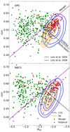 |
Fig. 22. Gini vs M20 coefficients for the DPS (top panel) and the NBCS (lower panel). Blue (resp. orange) contours represent galaxies classified as LTG (resp. S0) and red (resp. green) dots denote elliptical (resp. merger) galaxies (See the classification in Sect. 3.2). The purple line separates galaxies classified as merger on the left hand side and galaxies associated with a Hubble type on the right hand side (Lotz et al. 2004). The lower black dashed line divides elliptical, S0 and Sa galaxies from later types namely Sb, Sc and Irr (Lotz et al. 2008). |
Galaxies of the DPS and the NBCS, classified as merger or elliptical, show good agreement between their classification and their position on the Gini-M20 diagram (Fig. 22). Galaxies classified as S0 are spread over the region of early and late Hubble types with similar distributions between the DPS and the NBCS. This diagnostic diagram indicates a difference for LTG of the DPS in comparison to the NBCS: we observe that LTGs of the DPS are mainly (63%) situated in the region associated with earlier Hubble type galaxies, whereas LTGs of the NBCS are mainly situated in the region of later Hubble types (only 35% in the earlier Hubble type region). One might think that Sa galaxies are over-represented in the DPS. However, with respect to the full sample, we detect 10% of the DPS and 11% of the NBCS classified as Sa galaxies. We only find 6% of the DPS that are classified as Sb-d, whereas 19% of the NBCS are of this type. Hence, there is no Sa excess but a deficit of Sb-d galaxies. In Appendix C, we find Sb-d of the DPS to be the only morphological sub-sample that shows larger stellar masses (∼0.2 dex in log(M*/M⊙)) in comparison to LTG galaxies of the NBCS. Additionally, we find the highest difference in extinction of about 0.3 mag in the V band. We furthermore detect a significant excess in star formation in the centre: for Sb-d of the DPS (resp. NBCS), we find a median  (resp.
  ).
).
The shift towards earlier Hubble types of LTGs of the DPS, in comparison to the NBCS, is also supported by the measured Sérsic index, presented in Fig. 23. By comparing the Sérsic index of the DPS with those of the NBCS, we only find a discrepancy for LTGs, all other subsets show similar distributions. This indicates, that LTG of the DPS tend to have larger bulges in comparison to the LTGs of the NBCS.
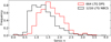 |
Fig. 23. Distribution of Sérsic indices, computed by STATMORPH (Rodriguez-Gomez et al. 2019) for the Legacy survey r-band images (Dey et al. 2019), of LTGs of the DPS (red line) and NBCS (black line). The areas under the histograms are normalised to unity. |
Interestingly, Nevin et al. (2019) tested the position of simulated minor and major mergers in the Gini-M20 diagram (see their Fig. 7) and found that most minor mergers and about half of the major mergers lie below the purple line, and mainly in the ETG/S0/Sa region (above the black dashed line). This corresponds to the trend discussed in Lotz et al. (2008): post-coalescence galaxies are more concentrated in their light distribution, while tidal features vanish.
In Appendix B, we follow Nevin et al. (2019), who developed a supervised Linear Decomposition Analysis (LDA) in order to compute the predictor coefficients LD1major and LD1minor, defined to identify major and minor mergers. To get comparable results, we restricted our analysis to z < 0.075. We find in cases, such as LTG and S0 galaxies, slightly higher merger rates for the DPS in comparison to the NBCS. This result somehow supports a merging scenario, while it is compatible with the fact DP galaxies might be dominated by post-coalescence mergers that would escape such analysis targeting on-going mergers. This result is compatible with the results discussed above based on the Gini-M20 diagram.
4.6. Summary
We have studied different parameters derived from observations to compare the DPS with the NBCS. The NBCS is defined to have the same redshift and stellar mass distributions as the DPS (see Sect. 2.3).
We find the following similar properties:
– Distributions of absolute magnitudes, stellar ages, metallicities, specific star formation ratio and [OIII]λ5008 emission line luminosities are identical.
– According to their colour-colour and their specific star formation-stellar mass diagrams, most of DPS and NBCS galaxies follow the star forming main sequence, only a few exhibit a quenched SF and some are located in the red sequence.
– Double-AGN behave as NBCS-AGN with respect to star formation: there is no significant central excess.
– If one considers that each peak corresponds to a component, the DPS and NBCS follow the Tully-Fisher relation.
– Elliptical galaxies from DPS and NBCS follow the Faber-Jackson relation.
– The same environment statistics are found for the DPS and the NBCS. Most of S0s are isolated, and the S0s excess observed in the DPS is not due to environment.
We detect the following differences:
– There is an excess of S0s (resp. a deficit of LTGs) in the DPS with respect to the NBCS.
– According to the Gini-M20 diagram, there appears to also be an excess of Sa galaxies in the DPS compared to the NBCS.
– LTG galaxies display higher Sérsic indices in the DPS compared to those in the NBCS.
– Galaxies classified as LINER are less common in the DPS in comparison to the NBCS.
– DPS galaxies show slightly higher absolute luminosities in the Hαλ6565 emission line.
– Double-SF galaxies exhibit a central starburst stronger than SF galaxies from the NBCS.
– Double-COMP, -LTG and -S0 galaxies also have such an excess but less significant.
– Double-COMP are more likely SF galaxies, according to the [OII]λ3728/[OIII]λ5008 line ratio, and to the detection rate of the high-ionisation [NeV]λ3426 emission line at z > 0.2.
– There is slightly more extinction (0.25 mag in V) in DPS galaxies than in their NBCS counterparts.
– All DPS velocity estimators are independent of the inclination, while we do detect a correlation for the NBCS.
– At given stellar masses, stellar velocity dispersions are larger for the DPS than for the NBCS.
– The gas velocity dispersion estimator of the close peak component of the DPS is compatible with velocity dispersions measured for the NBCS, whereas the far peak component of the DPS is not.
– With a single Gaussian approximation, the LTG and S0 galaxies from the DPS are offset from the NBCS TF relation.
– S0 galaxies from the DPS are shifted on the FJ relation from the NBCS.
5. Discussion
In Sect. 5.1, we argue that S0 galaxies detected as gas-rich DP galaxies belong to a star-forming population identified in previous works. In Sect. 5.2, we discuss how our non-parametric analysis revealed that LTG are dominated by Sa galaxies in the DPS. In Sect. 5.3, we propose that the DP galaxies sample is a minor merger sequence which could explain the different results discuss in Sect. 4.6. In Sect. 5.4, we discuss here different observations, which are compatible with the characteristics of the DPS described as a minor merger sequence. In Sect. 5.5, we compare the known properties of the DPS galaxies with respect to those of minor and major mergers. To present a complete discussion, we discuss further explanations of the observation of DP in Sect. 5.6 and find that these only apply to a few galaxies in our sample.
5.1. Star-forming S0s
S0 galaxies are usually described as disc galaxies, which have exhausted their gas content (e.g. Somerville & Davé 2015) and are proposed as a parallel Hubble sequence (van den Bergh 1976; Kormendy & Bender 2012). However, it has been known for several decades that some S0s are not forming stars but host large amounts of HI gas (e.g. Kennicutt 1989). In these early observations of HI-gas-rich S0 galaxies (e.g. van Woerden et al. 1983; Knapp et al. 1984, 1985; Krumm et al. 1985; van Driel et al. 1988), inner and outer rings were already detected, and analysed in simulations (e.g. Athanassoula & Bosma 1985; Buta & Combes 1996). The HI gas has often an Hα − [NII]-counterpart (e.g. Pogge & Eskridge 1993). Observations have shown indeed that about 85% of S0 galaxies host optical ionised gas (e.g. Macchetto et al. 1996; Sarzi et al. 2006) and 72% of those are isolated (Katkov et al. 2015). Kannappan et al. (2009) identified a blue sequence of SF S0 galaxies in the low-mass range that might be fading mergers, while massive S0s, with M > 2 × 10¹¹ M⊙, belong to the red sequence, but up to 2% of these massive S0 are SF. In the blue S0 sequence, they identify central blue colour gradients, which are interpreted as reminiscent of mergers (e.g. Kannappan 2004; Kewley et al. 2006a). Xiao et al. (2016) find about 8% of an S0 sample exhibits central star formation. They also found that the majority of these SF S0 galaxies have a stellar mass below 1010.6 M⊙. Tous et al. (2020) did not find such a mass separation. In their study of these two S0 populations composed of SF and quiescent galaxies, they found that SF S0 galaxies avoid high-galaxy density and that their SFR and spectral characteristics are entirely similar to those seen in LTGs.
Numerous observations show further evidence of various tidal disturbances in the outer parts of S0: outer rings (e.g. Comerón et al. 2014; Sil’chenko et al. 2018), polar rings (e.g. van Gorkom et al. 1987; Whitmore et al. 1990), circum-nuclear polar rings (e.g. Sil’chenko & Afanasiev 2004; Chilingarian et al. 2009; Sil’chenko 2016), counter-rotations (e.g. Katkov et al. 2013, 2014; Ilyina et al. 2014; Katkov et al. 2015, 2016; Pizzella et al. 2018) and cylindrical rotation (e.g. Molaeinezhad et al. 2019). In Katkov et al. (2014, 2015), Proshina et al. (2019), and Sil’chenko et al. (2019), the authors discuss the origin of this counter-rotating gas and argue that S0s might accrete gas probably from filaments or from minor mergers. In parallel, numerous works have shown that S0s can be produced by galaxy mergers including major mergers (Bekki 1998; Querejeta et al. 2015; Tapia et al. 2017; Eliche-Moral et al. 2018) as well as minor mergers (Bournaud et al. 2005; Bekki & Couch 2011).
Here, we clearly detect intermediate-mass S0 galaxies in the mass range 3 × 10¹⁰ − 3 × 10¹¹ M⊙ with optical ionised gas, including a large fraction of star forming galaxies. Beside their optical morphology, their kinematic behaviour is similar to those of LTGs. We find similar distributions for LTGs and S0 galaxies in the TFR in Sect. 4.3.4. We argue that the close peak might represent the central galaxy, while the far peak might correspond to a smaller companion or to the result of a recent gas accretion.
5.2. Non-parametric merger identification
In the Sect. 4.5, we compute several non-parametric diagnostics such as CAS-statistics, the shape asymmetry As, the Gini and M20 coefficients and the Sérsic index n to investigate different approaches of merger identification.
Morphological asymmetry is more prevalent in galaxies within close pairs (Patton et al. 2016). Moreover, SF is enhanced in close pairs with small differences in line-of-sight velocities (Patton et al. 2011, 2013). We studied galaxy asymmetries in the DPS, relying on the parameters of Patton et al. (2016). We do not find any asymmetry difference between the DPS and the NBCS nor any connection between SF and asymmetry. In a scenario where the central SF enhancement is due to a merging process, the absence of a significant asymmetry in the DPS would favour later stages of merging processes or mergers hidden inside the fibre. Pawlik et al. (2016) introduced the shape asymmetry to identify later stages of merger in comparison to the asymmetry. We do not find any difference between the DPS and the NBCS using this diagnostics.
We conducted a merger selection based on the Gini-M20 disgnostics, proposed by Lotz et al. (2004, 2008) to separate mergers from non-mergers and to distinguish between late and early Hubble types. We find good agreements with the predictions for S0, merger and elliptical galaxies of the DPS and the NBCS. LTGs of the DPS reveal a systematic effect: they are situated in the region of earlier Hubble types in comparison to LTGs of the NBCS (see Fig. 22). This is in agreement with the fact that we find a tendency towards higher Sérsic index n for LTGs of the DPS in comparison to the NBCS, supporting the idea of a sequence of galaxies thickening towards S0. Last, this is in agreement with the trend discussed in Appendix B with the small positive bias for minor and major mergers observed in the predictor coefficient distributions, as defined by Nevin et al. (2019). These authors also show that numerous simulated (major and minor) mergers lie in the non-merger regions of the Gini-M20 diagram.
Comparing all non-parametric methods, designed to detect merger rates, we do not find a direct relation between on-going mergers and DP structure at z < 0.075. Even though, these diagnostics were developed to detect late and post-coalescence stages of mergers (Pawlik et al. 2016; Lotz et al. 2008, 2010b,a; Nevin et al. 2019), we might see an even later stage, where traces such as fading tidal features are already quite weak and double nucleus beyond spatial resolution. Nevin et al. (2019) defined post-coalescence when the two galactic nuclei are separated by less than 1 kpc, which correspond to the SDSS resolution at z ≤ 0.03. Indeed as the DP feature is based on the central 3″ spectra, it is probable that the discussed diagnostics are not sensitive.
5.3. S0s as a part of the minor merger sequence
Walker et al. (1996) found that in 1:10 minor mergers, the discs are not destroyed but evolve to an earlier Hubble type, while a core of 45% of the satellite initial mass can reach the central kpc in 1 Gyr. This scenario might account for our DPS: high stellar velocity dispersions, two gas components and a similar kinematic behaviour for the different morphological types. This is supported by numerous hydrodynamical simulations. Bournaud et al. (2005) showed that intermediate mergers with 1:4 to 1:10 mass ratio can produce S0 galaxies. A similar situation was observed in GALMER simulations (Chilingarian et al. 2010a). Hence, while it is now well-known that S0s can be formed by minor and major mergers depending on the orientation and kinematics, Bournaud et al. (2007) studied the evolution of galaxies due to repeated minor mergers, as expected in the hierarchical growth of galaxies. Multiple sequential mergers feed the main progenitor, and gradually change its morphology from a spiral to an elliptical-like system. In addition, this is compatible with the work of van Dokkum et al. (2015) who proposed a two-channel evolution scheme, to account for the evolution of mass-size relation: they first grow inside-out with gas accretion and gas-rich minor mergers, until they quench, and continue to grow by dry minor mergers. Cappellari (2013) proposed a similar modelling to account for the evolution of slow and fast rotators, as further discussed in Cappellari (2016). This scenario is fully compatible with the properties of Sa and S0 galaxies and such a sequential gas-rich minor merger sequence accounts for the main properties of the DPS galaxies, identified here.
The increased central star formation and enhanced central extinction are also well accounted for by minor mergers and galaxy-galaxy interactions (e.g. Li et al. 2008; Ellison et al. 2011a). Using hydrodynamical simulations, Mapelli et al. (2015) produced rejenuvated S0 galaxies and a central SF enhancement with minor mergers with gas-rich galaxies. More generally, this work is compatible with the results of Li et al. (2008), who find that the majority of galaxies with high SSFR have a companion or exhibit tidal features.
5.4. Support from other observations
Studies of S0s performed with planetary nebulae provide characteristics comparable with our findings on the TF relation. With a spectroscopic and kinematic analysis of planetary nebulae in six S0 galaxies, Cortesi et al. (2013) found that S0s are supported by random motions in addition to their rotating discs. S0 galaxies lie about 1 magnitude below the TFR for spiral galaxies while their spheroids lie 1 magnitude above the FJR for elliptical galaxies. This supports previous findings on these S0 characteristics (Bedregal et al. 2006; Rawle et al. 2013), which we observe in the DPS for S0s but also for LTGs. Davis et al. (2016) also observed a break for high velocities in the TF relation, which they interpret as an additional baryonic mass present in the central part.
Similarly to Kannappan et al. (2009), Bait et al. (2017) and Fraser-McKelvie et al. (2018) identified two separate populations of S0 galaxies. Beside old, massive and metal rich galaxies with a bulge older than the disc (probably due to an inside-out quenching), they discuss less massive and more metal poor population having bulges with more recent star formation than their disc. They might have undergone a bulge rejuvenation (or disc fading), or compaction. They argued that environment is not playing a major role, and proposed a faded spiral scenario, which forms low mass S0s while other processes such as mergers form the more massive S0s. As we only detect massive S0s, this is compatible with our findings. We have a population of massive star-forming galaxies, which are evolving through different stages of mergers. S0 galaxies represent 36% of the whole DP population, they are not faded. Beside their morphology, we cannot disentangle them from LTGs.
5.5. Minor versus major mergers
As discussed in Bournaud et al. (2005), intermediate mass mergers with ratio 1:4–1:10 produce Sa to S0 galaxies, while equal mass mergers produce mainly ellipticals (e.g. Barnes & Hernquist 1991), and 1:3–1:4 can produce S0-like systems (e.g. Bekki 1998; Eliche-Moral et al. 2018). Last, the scenario of single minor mergers, with mass ratio larger than 1:10, produces spiral galaxies, while sequential multiple minor mergers can also lead to Sa/S0 galaxies (Bournaud et al. 2007).
On the one hand, the fact that the two peaks have typical intensity ratio in the range 1−3 might favour the idea of two galaxy nuclei with progenitors with 1:1–1:4 mass ratios. However, the absence of differences in the rate of morphological mergers between DPS and NBCS is not expected if the majority were such major mergers, as well as the absence of any differences in the distribution of shape-asymmetry and asymmetry. Major mergers can produce large starbursts (e.g. Barnes & Hernquist 1991), even though this is not always the case (e.g. Di Matteo et al. 2007). However, Hani et al. (2020) found that strong enhancements of SFR are dominated by major mergers. They estimated that a starburst of 50 M⊙ yr−1 has four times higher chances to occur in a major merger than in a minor merger. We have here 1.3% of the sample with a SFR larger than 50 M⊙ yr−1.
On the other hand, as discussed above multiple sequential gas-rich minor mergers and/or gas accretion might also produce the DPS galaxies (e.g. Walker et al. 1996). They could also account for the excess of S0 galaxies and the prevalence of Sa galaxies in LTG, as well as relatively morphologically regular DPS galaxies (Mazzilli-Ciraulo et al., in prep.). The intensity ratio of the two peaks (between 1 and 3) can also be biased by the excitation of the AGN triggered by a merger (Maschmann et al., in prep.).
As discussed in Appendix C, the 0.2 dex higher typical stellar masses of DPS galaxies, their 0.25 mag typical excess extinction in V and their central enhancement of star formation for Sb-d galaxies, all in comparison to the NBCS, suggest a past merger scenario for them. A visual inspection of the selected galaxies reveals that they are not dominated by edge-on or strongly inclined galaxies. However, Sb-d galaxies constitute 6% of the DPS (19% of the NBCS).
As discussed by Hani et al. (2020) and references therein, minor mergers are expected much more numerous than major ones, for example Kaviraj (2014) estimated that 40% of SF observed in local spirals is directly triggered by minor mergers. In addition, major mergers are known to trigger stronger SF than their minor counterparts. The distributions of SFRfibre estimated in the SF-DPS galaxies peak between 2 and 10 M⊙ yr−1 and is about a factor of 2 larger than for the NBCS. In numerical simulations, Hani et al. (2020) found an SFR enhancement of a factor two in 10.0 ≤ log(M*/M⊙) ≤ 11.4 SF post-merger galaxies.
Elliptical galaxies of the DPS are situated in the star forming main sequence (see Sect. 4.2), whereas their counterparts of the NBCS are quenched. We quantify this in Appendix C: elliptical DP galaxies show a 4 times higher SFR in comparison to single peaked elliptical galaxies. We furthermore find that elliptical galaxies with a DP have on average a 3 Gyr younger stellar population in comparison with those showing a single peak. This is consistent with the detection of molecular gas in star forming early type galaxies by Combes et al. (2007), who conclude that the molecular gas might has been accreted from the environment and shows properties rather independent from the old, pre-existing stellar component. Such a recent gas accretion might explain the emission line shape and the ongoing star formation that we detect.
DP galaxies have numerous characteristics of post-mergers with enhanced central star formation and extinction. The nature of the DP feature is still elusive, and could correspond to gas clumps as well as to relics of two galaxy nuclei. We argue that DPS galaxies, most of which exhibit an ordinary morphology, are more likely to be linked to gas-rich minor mergers or gas accretion than to major mergers, which would impact more strongly their morphologies. Indeed, we do detect the same number of morphological mergers in the DPS and NBCS. The sequential multiple minor merger scenario accounts for the S0 morphological excess clearly detected in the DPS, while we cannot exclude that a few of these DP galaxies originate from major mergers.
5.6. Alternatives
Supermassive black holes hosted in galaxy centres are expected to have a significant feedback during the AGN phase (Fabian 2012). This effect is measured to be stronger in massive galaxies (Somerville & Davé 2015; Zhang et al. 2018), than in smaller galaxies dominated by star formation feedback. Galaxy collisions are usually thought to trigger AGN feedback (Di Matteo et al. 2005). Gas outflow are found to be associated to emission line asymmetries (Heckman et al. 1981; Whittle 1985). This is studied on large data samples with fitting procedures using single- and double-Gaussian functions in for example Greene & Ho (2005) and Woo et al. (2016). Using observations based on spectroscopic integral field units, Karouzos et al. (2016) observed AGN driven outflow components with velocities between 300 and 600 km s−1 with velocity dispersion up to 800 km s−1. In the study on major mergers, Rupke & Veilleux (2013) have shown that galaxies with a QSO have the highest projected outflow velocities of at least 1450 km s−1. In the system F08572+3915:NW, they found velocities up to 3350 km s−1. Galaxies without an AGN still reach projected velocities up to 1000 km s−1. They concluded that QSOs play a key role in accelerating gas outflows. Beside these extreme velocities, an outflow with low projected velocities of several hundred km s−1 has been observed in NGC 5929 (Riffel et al. 2014).
In order to discuss an AGN outflow creating emission lines with a DP structure, we selected galaxies with a broader off-centred emission line component. Therefore, these galaxies have one peak component associated with the stellar velocity, computed by Chilingarian et al. (2017) and a second peak component more offset in units of σ1, 2 (as discussed in Sect. 4.3.1). Furthermore, we demanded the second peak component to show a velocity dispersion larger than 200 km s−1 which is similar to lower velocity dispersion of the outflow component found by Karouzos et al. (2016). We thus selected 68 galaxies showing a broad off-centred component as described in the discussed literature above. We show an example in the upper panel of Fig. 1.
Using the non-parametric emission line for the BPT classification (see Sect. 3.1), we find only 1% of these outflow candidates to be classified as SF galaxies. We find 50% to be classified as AGN, 24% as COMP and 13% as LINER. Even though we find a connection to AGN activity for outflow candidates, these galaxies make only about 1% of the DPS. The lack of sensitivity to AGN outflow candidates can be explained by the amplitude criteria 1/3 < A1/A2 < 3 applied in the selection procedure (see Sect. 2.2). Outflow components show mostly very broad component with a lower amplitude described as wings (e.g Heckman et al. 1981; Whittle 1985; Greene & Ho 2005). These types of asymmetries are systematically filtered out in this work.
We also discussed an outflow scenario to explain off-centred weak [OIII]λ5008 in Maschmann & Melchior (2019). In summary, we find evidence for AGN-driven gas outflow in some galaxies, but in comparison to the large sample of DP galaxies we conclude that this scenario provides well-suited arguments only for a small fraction of them.
6. Conclusions
We identified double-peak emission line galaxies with an automated procedure. They are quite rare as they constitute 0.8% of the RCSED/SDSS catalogue. We compared the DP galaxies with their counter-parts from the no-bias control sample and find several significant differences. There is an excess of S0 galaxies, which cannot be accounted for by the environment. The S0-DP galaxies correspond to the star-forming S0 galaxies identified in isolated environments as discussed in Tous et al. (2020). In parallel, the Gini-M20 diagram reveals that LTG are mainly Sa galaxies in the DPS with respect to the LTG of the NBCS. Similarly, the DP LTG exhibit a larger Sérsic index than their NBCS counterparts.
On the one hand, we find that LTG and S0 galaxies behave similarly on the TF relation but are off-centred towards large velocity dispersions. On the other hand, if two gas components are considered, we show that the close component behaves as expected while the far peak is offset and might correspond to a smaller component or a large gas clump. Other results further support this scenario: (1) the absence of any dependency on the galaxy inclination, (2) larger stellar velocity dispersions, (3) a systematic central enhancement of star formation and (4) a central enhancement of the extinction.
We argue that this double-peak sample constitutes a sequence of multiple sequential minor mergers, which could explain the similar behaviour observed for the different morphological types. It is a sequence in the sense that the impact of sequential minor mergers is to increase the size of the bulge, leading to larger fractions of S0 galaxies, while the majority of disc galaxies are Sa. It is difficult to disentangle gas-rich minor mergers from gas accretion, but both will have similar effects. The absence of an excess of proper morphological mergers supports the view that the impact is small, typical of minor mergers. The specificity of these DP galaxies is that the spectroscopic signature is inside the 3″ SDSS-fibre, hence, it is somehow a post-coalescence stage not detected in morphological studies. Last, this sample also constitutes a time sequence of mergers as their spread in redshift gathers galaxies observed with resolution between 1 kpc and 12 kpc.
© Copyright CERN 2014-18 (http://root.cern.ch/).
We refer throughout this article to LTG for all disc galaxies from Sa to Sd.
We used the galaxy group catalogue compiled on the SDSS DR 7 available under: https://gax.sjtu.edu.cn/data/Group.html
Acknowledgments
This work is based on the master thesis of DM. We acknowledge Françoise Combes, Anaëlle Halle, Barbara Mazzilli-Ciraulo and Anton Afanasiev for fruitful discussions. We thank the anonymous referee for suggestions on further investigating in non-parametric morphological diagnostics and enlarging the discussion on the merger rate, which supported our analysis and made it more solid. We thank Ivan Zolotukhin for his support in the early stage of this work. D. M. thanks Gabriele Gramelsberger, Dawid Kasprowicz, Lisa Schüttler, Daniel Wenz, Lukas Böhres and Frederic Kerksieck for supporting this work and for constructive discussions on software structure. We thank David Patton for providing the asymmetry parameter for SDSS galaxies and Helena Domínguez-Sánchez and Kanak Saha for helping with the morphological classification. We also thank Marina Trevisan for nice feedback on the discussion. IC is supported by Telescope Data Center at Smithsonian Astrophysical Observatory. I.C. and I.K. acknowledge the Russian Science Foundation Grant 19-12-00281 and the Program of development of M.V. Lomonosov Moscow State University for the Leading Scientific School “Physics of stars, relativistic objects and galaxies”. Rene Brun and Fons Rademakers, ROOT – An Object Oriented Data Analysis Framework, Proceedings AIHENP’96 Workshop, Lausanne, Sep. 1996, Nucl. Inst. & Meth. in Phys. Res. A 389 (1997) 81–86. See also http://root.cern.ch/. Funding for the Sloan Digital Sky Survey IV has been provided by the Alfred P. Sloan Foundation, the US Department of Energy Office of Science, and the Participating Institutions. SDSS-IV acknowledges support and resources from the Center for High-Performance Computing at the University of Utah. The SDSS web site is www.sdss.org. SDSS-IV is managed by the Astrophysical Research Consortium for the Participating Institutions of the SDSS Collaboration including the Brazilian Participation Group, the Carnegie Institution for Science, Carnegie Mellon University, the Chilean Participation Group, the French Participation Group, Harvard-Smithsonian Center for Astrophysics, Instituto de Astrofísica de Canarias, The Johns Hopkins University, Kavli Institute for the Physics and Mathematics of the Universe (IPMU)/University of Tokyo, the Korean Participation Group, Lawrence Berkeley National Laboratory, Leibniz Institut für Astrophysik Potsdam (AIP), Max-Planck-Institut für Astronomie (MPIA Heidelberg), Max-Planck-Institut für Astrophysik (MPA Garching), Max-Planck-Institut für Extraterrestrische Physik (MPE), National Astronomical Observatories of China, New Mexico State University, New York University, University of Notre Dame, Observatário Nacional/MCTI, The Ohio State University, Pennsylvania State University, Shanghai Astronomical Observatory, United Kingdom Participation Group, Universidad Nacional Autónoma de México, University of Arizona, University of Colorado Boulder, University of Oxford, University of Portsmouth, University of Utah, University of Virginia, University of Washington, University of Wisconsin, Vanderbilt University, and Yale University. The Legacy Surveys (http://legacysurvey.org/) consist of three individual and complementary projects: the Dark Energy Camera Legacy Survey (DECaLS; NOAO Proposal ID # 2014B-0404; PIs: David Schlegel and Arjun Dey), the Beijing-Arizona Sky Survey (BASS; NOAO Proposal ID # 2015A-0801; PIs: Zhou Xu and Xiaohui Fan), and the Mayall z-band Legacy Survey (MzLS; NOAO Proposal ID # 2016A-0453; PI: Arjun Dey). DECaLS, BASS and MzLS together include data obtained, respectively, at the Blanco telescope, Cerro Tololo Inter-American Observatory, National Optical Astronomy Observatory (NOAO); the Bok telescope, Steward Observatory, University of Arizona; and the Mayall telescope, Kitt Peak National Observatory, NOAO. The Legacy Surveys project is honoured to be permitted to conduct astronomical research on Iolkam Du‘ag (Kitt Peak), a mountain with particular significance to the Tohono O’odham Nation.
References
- Abazajian, K. N., Adelman-McCarthy, J. K., Agüeros, M. A., et al. 2009, ApJS, 182, 543 [NASA ADS] [CrossRef] [Google Scholar]
- Abraham, R. G., van den Bergh, S., & Nair, P. 2003, ApJ, 588, 218 [NASA ADS] [CrossRef] [Google Scholar]
- Acker, A., Köppen, J., Samland, M., & Stenholm, B. 1989, Messenger, 58, 44 [Google Scholar]
- Aquino-Ortíz, E., Valenzuela, O., Sánchez, S. F., et al. 2018, MNRAS, 479, 2133 [NASA ADS] [CrossRef] [Google Scholar]
- Athanassoula, E., & Bosma, A. 1985, ARA&A, 23, 147 [CrossRef] [Google Scholar]
- Avila-Reese, V., Zavala, J., Firmani, C., & Hernández-Toledo, H. M. 2008, AJ, 136, 1340 [NASA ADS] [CrossRef] [Google Scholar]
- Bait, O., Barway, S., & Wadadekar, Y. 2017, MNRAS, 471, 2687 [NASA ADS] [CrossRef] [Google Scholar]
- Baldwin, J. A., Phillips, M. M., & Terlevich, R. 1981, PASP, 93, 5 [NASA ADS] [CrossRef] [EDP Sciences] [Google Scholar]
- Balogh, M. L., Schade, D., Morris, S. L., et al. 1998, ApJ, 504, L75 [NASA ADS] [CrossRef] [Google Scholar]
- Barnes, J. E., & Hernquist, L. E. 1991, ApJ, 370, L65 [NASA ADS] [CrossRef] [Google Scholar]
- Bedregal, A. G., Aragón-Salamanca, A., & Merrifield, M. R. 2006, MNRAS, 373, 1125 [NASA ADS] [CrossRef] [Google Scholar]
- Begelman, M. C., Blandford, R. D., & Rees, M. J. 1980, Nature, 287, 307 [NASA ADS] [CrossRef] [Google Scholar]
- Bekki, K. 1998, ApJ, 502, L133 [NASA ADS] [CrossRef] [Google Scholar]
- Bekki, K., & Couch, W. J. 2011, MNRAS, 415, 1783 [NASA ADS] [CrossRef] [Google Scholar]
- Blanton, M. R., & Moustakas, J. 2009, ARA&A, 47, 159 [NASA ADS] [CrossRef] [Google Scholar]
- Bond, J. R., Kofman, L., & Pogosyan, D. 1996, Nature, 380, 603 [NASA ADS] [CrossRef] [Google Scholar]
- Bothun, G. D., & Dressler, A. 1986, ApJ, 301, 57 [NASA ADS] [CrossRef] [Google Scholar]
- Bournaud, F., Jog, C. J., & Combes, F. 2005, A&A, 437, 69 [NASA ADS] [CrossRef] [EDP Sciences] [Google Scholar]
- Bournaud, F., Jog, C. J., & Combes, F. 2007, A&A, 476, 1179 [NASA ADS] [CrossRef] [EDP Sciences] [Google Scholar]
- Brinchmann, J., Charlot, S., White, S. D. M., et al. 2004, MNRAS, 351, 1151 [NASA ADS] [CrossRef] [Google Scholar]
- Buta, R., & Combes, F. 1996, Fund. Cosmic Phys., 17, 95 [Google Scholar]
- Calistro Rivera, G., Williams, W. L., Hardcastle, M. J., et al. 2017, MNRAS, 469, 3468 [NASA ADS] [CrossRef] [Google Scholar]
- Cappellari, M. 2013, ApJ, 778, L2 [NASA ADS] [CrossRef] [Google Scholar]
- Cappellari, M. 2016, ARA&A, 54, 597 [NASA ADS] [CrossRef] [Google Scholar]
- Catinella, B., Haynes, M. P., & Giovanelli, R. 2005, AJ, 130, 1037 [NASA ADS] [CrossRef] [Google Scholar]
- Catinella, B., Kauffmann, G., Schiminovich, D., et al. 2012, MNRAS, 420, 1959 [NASA ADS] [CrossRef] [Google Scholar]
- Chilingarian, I. V., & Zolotukhin, I. Y. 2012, MNRAS, 419, 1727 [NASA ADS] [CrossRef] [Google Scholar]
- Chilingarian, I. V., Novikova, A. P., Cayatte, V., et al. 2009, A&A, 504, 389 [NASA ADS] [CrossRef] [EDP Sciences] [Google Scholar]
- Chilingarian, I. V., Melchior, A.-L., & Zolotukhin, I. Y. 2010a, MNRAS, 405, 1409 [NASA ADS] [CrossRef] [Google Scholar]
- Chilingarian, I. V., Di Matteo, P., Combes, F., Melchior, A. L., & Semelin, B. 2010b, A&A, 518, A61 [NASA ADS] [CrossRef] [EDP Sciences] [Google Scholar]
- Chilingarian, I. V., Zolotukhin, I. Y., Katkov, I. Y., et al. 2017, ApJS, 228, 14 [NASA ADS] [CrossRef] [Google Scholar]
- Chilingarian, I. V., Katkov, I. Y., Zolotukhin, I. Y., et al. 2018, ApJ, 863, 1 [CrossRef] [Google Scholar]
- Combes, F., Young, L. M., & Bureau, M. 2007, MNRAS, 377, 1795 [NASA ADS] [CrossRef] [Google Scholar]
- Comerford, J. M., Gerke, B. F., Newman, J. A., et al. 2009, ApJ, 698, 956 [NASA ADS] [CrossRef] [Google Scholar]
- Comerford, J. M., Gerke, B. F., Stern, D., et al. 2012, ApJ, 753, 42 [NASA ADS] [CrossRef] [Google Scholar]
- Comerford, J. M., Schluns, K., Greene, J. E., & Cool, R. J. 2013, ApJ, 777, 64 [CrossRef] [Google Scholar]
- Comerford, J. M., Pooley, D., Barrows, R. S., et al. 2015, ApJ, 806, 219 [Google Scholar]
- Comerford, J. M., Nevin, R., Stemo, A., et al. 2018, ApJ, 867, 66 [Google Scholar]
- Comerón, S., Salo, H., Laurikainen, E., et al. 2014, A&A, 562, A121 [NASA ADS] [CrossRef] [EDP Sciences] [Google Scholar]
- Condon, J. J. 1992, ARA&A, 30, 575 [NASA ADS] [CrossRef] [MathSciNet] [Google Scholar]
- Conselice, C. J. 2003, ApJS, 147, 1 [NASA ADS] [CrossRef] [Google Scholar]
- Cortesi, A., Merrifield, M. R., Coccato, L., et al. 2013, MNRAS, 432, 1010 [NASA ADS] [CrossRef] [Google Scholar]
- Cui, J., Xia, X. Y., Deng, Z. G., Mao, S., & Zou, Z. L. 2001, AJ, 122, 63 [NASA ADS] [CrossRef] [Google Scholar]
- Davis, T. A., Greene, J., Ma, C.-P., et al. 2016, MNRAS, 455, 214 [NASA ADS] [CrossRef] [Google Scholar]
- De Propris, R., Liske, J., Driver, S. P., Allen, P. D., & Cross, N. J. G. 2005, AJ, 130, 1516 [NASA ADS] [CrossRef] [Google Scholar]
- Deane, R. P., Paragi, Z., Jarvis, M. J., et al. 2014, Nature, 511, 57 [NASA ADS] [CrossRef] [Google Scholar]
- Dey, A., Schlegel, D. J., Lang, D., et al. 2019, AJ, 157, 168 [NASA ADS] [CrossRef] [Google Scholar]
- Di Matteo, T., Springel, V., & Hernquist, L. 2005, Nature, 433, 604 [NASA ADS] [CrossRef] [PubMed] [Google Scholar]
- Di Matteo, P., Combes, F., Melchior, A. L., & Semelin, B. 2007, A&A, 468, 61 [NASA ADS] [CrossRef] [EDP Sciences] [Google Scholar]
- Domínguez, A., Siana, B., Henry, A. L., et al. 2013, ApJ, 763, 145 [NASA ADS] [CrossRef] [Google Scholar]
- Domínguez Sánchez, H., Huertas-Company, M., Bernardi, M., Tuccillo, D., & Fischer, J. L. 2018, MNRAS, 476, 3661 [NASA ADS] [CrossRef] [Google Scholar]
- Dressler, A. 1980, ApJ, 236, 351 [NASA ADS] [CrossRef] [Google Scholar]
- Dressler, A., Oemler, A. Jr., Couch, W. J., et al. 1997, ApJ, 490, 577 [NASA ADS] [CrossRef] [Google Scholar]
- Drory, N., MacDonald, N., Bershady, M. A., et al. 2015, AJ, 149, 77 [NASA ADS] [CrossRef] [Google Scholar]
- Eliche-Moral, M. C., Rodríguez-Pérez, C., Borlaff, A., Querejeta, M., & Tapia, T. 2018, A&A, 617, A113 [NASA ADS] [CrossRef] [EDP Sciences] [Google Scholar]
- Elitzur, M., Asensio Ramos, A., & Ceccarelli, C. 2012, MNRAS, 422, 1394 [NASA ADS] [CrossRef] [Google Scholar]
- Ellis, S. C., Driver, S. P., Allen, P. D., et al. 2005, MNRAS, 363, 1257 [NASA ADS] [CrossRef] [Google Scholar]
- Ellison, S. L., Patton, D. R., Simard, L., & McConnachie, A. W. 2008, AJ, 135, 1877 [NASA ADS] [CrossRef] [Google Scholar]
- Ellison, S. L., Patton, D. R., Simard, L., et al. 2010, MNRAS, 407, 1514 [NASA ADS] [CrossRef] [Google Scholar]
- Ellison, S. L., Patton, D. R., Mendel, J. T., & Scudder, J. M. 2011a, MNRAS, 418, 2043 [NASA ADS] [CrossRef] [Google Scholar]
- Ellison, S. L., Nair, P., Patton, D. R., et al. 2011b, MNRAS, 416, 2182 [NASA ADS] [CrossRef] [Google Scholar]
- Faber, S. M., & Jackson, R. E. 1976, ApJ, 204, 668 [NASA ADS] [CrossRef] [Google Scholar]
- Fabian, A. C. 2012, ARA&A, 50, 455 [Google Scholar]
- Fasano, G., Poggianti, B. M., Couch, W. J., et al. 2000, ApJ, 542, 673 [NASA ADS] [CrossRef] [Google Scholar]
- Fisher, R. A. 1954, Statistical Methods for Research Eorkers, 20th ed. (Edinburgh: Oliver and Boyd) [Google Scholar]
- Fraser-McKelvie, A., Aragón-Salamanca, A., Merrifield, M., et al. 2018, MNRAS, 481, 5580 [NASA ADS] [CrossRef] [Google Scholar]
- Fu, H., Myers, A. D., Djorgovski, S. G., et al. 2015, ApJ, 799, 72 [NASA ADS] [CrossRef] [Google Scholar]
- Gallazzi, A., Charlot, S., Brinchmann, J., & White, S. D. M. 2006, MNRAS, 370, 1106 [NASA ADS] [CrossRef] [Google Scholar]
- Gao, H., Ho, L. C., Barth, A. J., & Li, Z.-Y. 2018, ApJ, 862, 100 [NASA ADS] [CrossRef] [Google Scholar]
- Ge, J.-Q., Hu, C., Wang, J.-M., Bai, J.-M., & Zhang, S. 2012, ApJS, 201, 31 [NASA ADS] [CrossRef] [Google Scholar]
- Genzel, R., Tacconi, L. J., Rigopoulou, D., Lutz, D., & Tecza, M. 2001, ApJ, 563, 527 [NASA ADS] [CrossRef] [Google Scholar]
- Gilli, R., Vignali, C., Mignoli, M., et al. 2010, A&A, 519, A92 [NASA ADS] [CrossRef] [EDP Sciences] [Google Scholar]
- Goulding, A. D., Pardo, K., Greene, J. E., et al. 2019, ApJ, 879, L21 [NASA ADS] [CrossRef] [Google Scholar]
- Green, P. J., Myers, A. D., Barkhouse, W. A., et al. 2010, ApJ, 710, 1578 [NASA ADS] [CrossRef] [Google Scholar]
- Greene, J. E., & Ho, L. C. 2005, ApJ, 627, 721 [NASA ADS] [CrossRef] [Google Scholar]
- Hani, M. H., Gosain, H., Ellison, S. L., Patton, D. R., & Torrey, P. 2020, MNRAS, 493, 3716 [CrossRef] [Google Scholar]
- Heckman, T. M., Miley, G. K., van Breugel, W. J. M., & Butcher, H. R. 1981, ApJ, 247, 403 [NASA ADS] [CrossRef] [Google Scholar]
- Helou, G., Soifer, B. T., & Rowan-Robinson, M. 1985, ApJ, 298, L7 [Google Scholar]
- Hogg, D. W., Blanton, M., Strateva, I., et al. 2002, AJ, 124, 646 [NASA ADS] [CrossRef] [Google Scholar]
- Ilyina, M. A., Sil’chenko, O. K., & Afanasiev, V. L. 2014, MNRAS, 439, 334 [NASA ADS] [CrossRef] [Google Scholar]
- Kannappan, S. J. 2004, ApJ, 611, L89 [NASA ADS] [CrossRef] [MathSciNet] [Google Scholar]
- Kannappan, S. J., Guie, J. M., & Baker, A. J. 2009, AJ, 138, 579 [NASA ADS] [CrossRef] [Google Scholar]
- Karouzos, M., Woo, J.-H., & Bae, H.-J. 2016, ApJ, 819, 148 [NASA ADS] [CrossRef] [Google Scholar]
- Katkov, I. Y., Sil’chenko, O. K., & Afanasiev, V. L. 2013, ApJ, 769, 105 [NASA ADS] [CrossRef] [Google Scholar]
- Katkov, I. Y., Sil’chenko, O. K., & Afanasiev, V. L. 2014, MNRAS, 438, 2798 [NASA ADS] [CrossRef] [Google Scholar]
- Katkov, I. Y., Kniazev, A. Y., & Sil’chenko, O. K. 2015, AJ, 150, 24 [NASA ADS] [CrossRef] [Google Scholar]
- Katkov, I. Y., Sil’chenko, O. K., Chilingarian, I. V., Uklein, R. I., & Egorov, O. V. 2016, MNRAS, 461, 2068 [NASA ADS] [CrossRef] [Google Scholar]
- Kauffmann, G., Heckman, T. M., White, S. D. M., et al. 2003, MNRAS, 341, 33 [NASA ADS] [CrossRef] [Google Scholar]
- Kaviraj, S. 2014, MNRAS, 440, 2944 [NASA ADS] [CrossRef] [Google Scholar]
- Kennicutt, R. C. Jr. 1989, ApJ, 344, 685 [NASA ADS] [CrossRef] [Google Scholar]
- Kewley, L. J., Dopita, M. A., Sutherland, R. S., Heisler, C. A., & Trevena, J. 2001, ApJ, 556, 121 [Google Scholar]
- Kewley, L. J., Geller, M. J., Jansen, R. A., & Dopita, M. A. 2002, AJ, 124, 3135 [NASA ADS] [CrossRef] [Google Scholar]
- Kewley, L. J., Groves, B., Kauffmann, G., & Heckman, T. 2006a, MNRAS, 372, 961 [NASA ADS] [CrossRef] [Google Scholar]
- Kewley, L. J., Geller, M. J., & Barton, E. J. 2006b, AJ, 131, 2004 [NASA ADS] [CrossRef] [Google Scholar]
- Knapp, G. R., van Driel, W., Schwarz, U. J., van Woerden, H., & Gallagher, J. S. I. 1984, A&A, 133, 127 [Google Scholar]
- Knapp, G. R., van Driel, W., & van Woerden, H. 1985, A&A, 142, 1 [NASA ADS] [Google Scholar]
- Kohandel, M., Pallottini, A., Ferrara, A., et al. 2019, MNRAS, 487, 3007 [NASA ADS] [CrossRef] [Google Scholar]
- Kormendy, J., & Bender, R. 2012, ApJS, 198, 2 [Google Scholar]
- Koss, M., Mushotzky, R., Treister, E., et al. 2012, ApJ, 746, L22 [Google Scholar]
- Koss, M. J., Glidden, A., Baloković, M., et al. 2016, ApJ, 824, L4 [NASA ADS] [CrossRef] [Google Scholar]
- Koss, M. J., Blecha, L., Bernhard, P., et al. 2018, Nature, 563, 214 [NASA ADS] [CrossRef] [Google Scholar]
- Krumm, N., van Driel, W., & van Woerden, H. 1985, A&A, 144, 202 [NASA ADS] [Google Scholar]
- Laigle, C., Pichon, C., Arnouts, S., et al. 2018, MNRAS, 474, 5437 [NASA ADS] [CrossRef] [Google Scholar]
- Lee, K.-G., Krolewski, A., White, M., et al. 2018, ApJS, 237, 31 [NASA ADS] [CrossRef] [Google Scholar]
- Li, C., Kauffmann, G., Heckman, T. M., Jing, Y. P., & White, S. D. M. 2008, MNRAS, 385, 1903 [NASA ADS] [CrossRef] [Google Scholar]
- Liu, X., Shen, Y., Strauss, M. A., & Greene, J. E. 2010, ApJ, 708, 427 [NASA ADS] [CrossRef] [Google Scholar]
- Liu, X., Shen, Y., Strauss, M. A., & Hao, L. 2011, ApJ, 737, 101 [NASA ADS] [CrossRef] [Google Scholar]
- Liu, X., Civano, F., Shen, Y., et al. 2013, ApJ, 762, 110 [NASA ADS] [CrossRef] [Google Scholar]
- Lotz, J. M., Primack, J., & Madau, P. 2004, AJ, 128, 163 [NASA ADS] [CrossRef] [Google Scholar]
- Lotz, J. M., Davis, M., Faber, S. M., et al. 2008, ApJ, 672, 177 [NASA ADS] [CrossRef] [Google Scholar]
- Lotz, J. M., Jonsson, P., Cox, T. J., & Primack, J. R. 2010a, MNRAS, 404, 575 [Google Scholar]
- Lotz, J. M., Jonsson, P., Cox, T. J., & Primack, J. R. 2010b, MNRAS, 404, 590 [NASA ADS] [CrossRef] [Google Scholar]
- Macchetto, F., Pastoriza, M., Caon, N., et al. 1996, A&AS, 120, 463 [NASA ADS] [CrossRef] [EDP Sciences] [Google Scholar]
- Mapelli, M., Rampazzo, R., & Marino, A. 2015, A&A, 575, A16 [NASA ADS] [CrossRef] [EDP Sciences] [Google Scholar]
- Maschmann, D., & Melchior, A.-L. 2019, A&A, 627, L3 [CrossRef] [EDP Sciences] [Google Scholar]
- Meert, A., Vikram, V., & Bernardi, M. 2015, MNRAS, 446, 3943 [NASA ADS] [CrossRef] [Google Scholar]
- Mendenhall, W., & Sincich, T. 2011, A Second Course in Statistics: Regression Analysis (Pearson Education) [Google Scholar]
- Mo, H. J., Mao, S., & White, S. D. M. 1998, MNRAS, 295, 319 [Google Scholar]
- Molaeinezhad, A., Zhu, L., Falcón-Barroso, J., et al. 2019, MNRAS, 488, 1012 [CrossRef] [Google Scholar]
- Müller-Sánchez, F., Comerford, J. M., Nevin, R., et al. 2015, ApJ, 813, 103 [NASA ADS] [CrossRef] [Google Scholar]
- Nevin, R., Comerford, J., Müller-Sánchez, F., Barrows, R., & Cooper, M. 2016, ApJ, 832, 67 [NASA ADS] [CrossRef] [Google Scholar]
- Nevin, R., Comerford, J. M., Müller-Sánchez, F., Barrows, R., & Cooper, M. C. 2018, MNRAS, 473, 2160 [NASA ADS] [CrossRef] [Google Scholar]
- Nevin, R., Blecha, L., Comerford, J., & Greene, J. 2019, ApJ, 872, 76 [NASA ADS] [CrossRef] [Google Scholar]
- Osterbrock, D. E., & Ferland, G. J. 2006, Astrophysics of Gaseous Nebulae and Active Galactic Nuclei (Sausalito, CA: University Science Books) [Google Scholar]
- Patton, D. R., Ellison, S. L., Simard, L., McConnachie, A. W., & Mendel, J. T. 2011, MNRAS, 412, 591 [NASA ADS] [CrossRef] [Google Scholar]
- Patton, D. R., Torrey, P., Ellison, S. L., Mendel, J. T., & Scudder, J. M. 2013, MNRAS, 433, L59 [NASA ADS] [CrossRef] [Google Scholar]
- Patton, D. R., Qamar, F. D., Ellison, S. L., et al. 2016, MNRAS, 461, 2589 [NASA ADS] [CrossRef] [Google Scholar]
- Pawlik, M. M., Wild, V., Walcher, C. J., et al. 2016, MNRAS, 456, 3032 [NASA ADS] [CrossRef] [Google Scholar]
- Petrosian, V. 1976, ApJ, 210, L53 [NASA ADS] [CrossRef] [Google Scholar]
- Pfeifle, R. W., Satyapal, S., Manzano-King, C., et al. 2019, ApJ, 883, 167 [CrossRef] [Google Scholar]
- Pimbblet, K. A., Smail, I., Kodama, T., et al. 2002, MNRAS, 331, 333 [NASA ADS] [CrossRef] [Google Scholar]
- Pizzella, A., Morelli, L., Coccato, L., et al. 2018, A&A, 616, A22 [CrossRef] [EDP Sciences] [Google Scholar]
- Pogge, R. W., & Eskridge, P. B. 1993, AJ, 106, 1405 [NASA ADS] [CrossRef] [Google Scholar]
- Proshina, I. S., Kniazev, A. Y., & Sil’chenko, O. K. 2019, AJ, 158, 5 [NASA ADS] [CrossRef] [Google Scholar]
- Querejeta, M., Eliche-Moral, M. C., Tapia, T., et al. 2015, A&A, 579, L2 [NASA ADS] [CrossRef] [EDP Sciences] [Google Scholar]
- Rawle, T. D., Lucey, J. R., Smith, R. J., & Head, J. T. C. G. 2013, MNRAS, 433, 2667 [NASA ADS] [CrossRef] [Google Scholar]
- Riffel, R. A., Storchi-Bergmann, T., & Riffel, R. 2014, ApJ, 780, L24 [NASA ADS] [CrossRef] [Google Scholar]
- Rodriguez-Gomez, V., Snyder, G. F., Lotz, J. M., et al. 2019, MNRAS, 483, 4140 [NASA ADS] [CrossRef] [Google Scholar]
- Rupke, D. S. N., & Veilleux, S. 2013, ApJ, 768, 75 [NASA ADS] [CrossRef] [Google Scholar]
- Salim, S. 2014, Serb. Astron. J., 189, 1 [Google Scholar]
- Salim, S., Rich, R. M., Charlot, S., et al. 2007, ApJS, 173, 267 [NASA ADS] [CrossRef] [Google Scholar]
- Salim, S., Lee, J. C., Janowiecki, S., et al. 2016, ApJS, 227, 2 [NASA ADS] [CrossRef] [Google Scholar]
- Sanders, D. B., & Mirabel, I. F. 1996, ARA&A, 34, 749 [NASA ADS] [CrossRef] [Google Scholar]
- Sarron, F., Adami, C., Durret, F., & Laigle, C. 2019, A&A, 632, A49 [NASA ADS] [CrossRef] [EDP Sciences] [Google Scholar]
- Sarzi, M., Falcón-Barroso, J., Davies, R. L., et al. 2006, MNRAS, 366, 1151 [Google Scholar]
- Saulder, C., van Kampen, E., Chilingarian, I. V., Mieske, S., & Zeilinger, W. W. 2016, A&A, 596, A14 [NASA ADS] [CrossRef] [EDP Sciences] [Google Scholar]
- Schawinski, K., Thomas, D., Sarzi, M., et al. 2007, MNRAS, 382, 1415 [NASA ADS] [CrossRef] [Google Scholar]
- Schiminovich, D., Wyder, T. K., Martin, D. C., et al. 2007, ApJS, 173, 315 [NASA ADS] [CrossRef] [Google Scholar]
- Schirmer, M., Diaz, R., Holhjem, K., Levenson, N. A., & Winge, C. 2013, ApJ, 763, 60 [NASA ADS] [CrossRef] [Google Scholar]
- Schneider, D. P., Richards, G. T., Hall, P. B., et al. 2010, AJ, 139, 2360 [NASA ADS] [CrossRef] [Google Scholar]
- Shimwell, T. W., Tasse, C., Hardcastle, M. J., et al. 2019, A&A, 622, A1 [NASA ADS] [CrossRef] [EDP Sciences] [Google Scholar]
- Sil’chenko, O. K. 2016, AJ, 152, 73 [CrossRef] [Google Scholar]
- Sil’chenko, O. K., & Afanasiev, V. L. 2004, AJ, 127, 2641 [NASA ADS] [CrossRef] [Google Scholar]
- Sil’chenko, O., Kostiuk, I., Burenkov, A., & Parul, H. 2018, A&A, 620, L7 [NASA ADS] [CrossRef] [EDP Sciences] [Google Scholar]
- Sil’chenko, O. K., Moiseev, A. V., & Egorov, O. V. 2019, ApJS, 244, 6 [NASA ADS] [CrossRef] [Google Scholar]
- Silk, J. 1997, ApJ, 481, 703 [NASA ADS] [CrossRef] [Google Scholar]
- Smith, K. L., Shields, G. A., Bonning, E. W., et al. 2010, ApJ, 716, 866 [NASA ADS] [CrossRef] [Google Scholar]
- Somerville, R. S., & Davé, R. 2015, ARA&A, 53, 51 [NASA ADS] [CrossRef] [EDP Sciences] [Google Scholar]
- Strateva, I., Ivezić, Ž., Knapp, G. R., et al. 2001, AJ, 122, 1861 [Google Scholar]
- Tammour, A., Gallagher, S. C., & Richards, G. 2015, MNRAS, 448, 3354 [CrossRef] [Google Scholar]
- Tapia, T., Eliche-Moral, M. C., Aceves, H., et al. 2017, A&A, 604, A105 [NASA ADS] [CrossRef] [EDP Sciences] [Google Scholar]
- Tous, J. L., Solanes, J. M., & Perea, J. D. 2020, MNRAS, 495, 4135 [CrossRef] [Google Scholar]
- Tremonti, C. A., Heckman, T. M., Kauffmann, G., et al. 2004, ApJ, 613, 898 [NASA ADS] [CrossRef] [Google Scholar]
- Tully, R. B., & Fisher, J. R. 1977, A&A, 54, 661 [NASA ADS] [Google Scholar]
- van den Bergh, S. 1976, ApJ, 206, 883 [NASA ADS] [CrossRef] [Google Scholar]
- van Dokkum, P. G., Nelson, E. J., Franx, M., et al. 2015, ApJ, 813, 23 [NASA ADS] [CrossRef] [Google Scholar]
- van Driel, W., van Woerden, H., Gallagher, J. S. I., & Schwarz, U. J. 1988, A&A, 191, 201 [Google Scholar]
- van Gorkom, J. H., Schechter, P. L., & Kristian, J. 1987, ApJ, 314, 457 [NASA ADS] [CrossRef] [Google Scholar]
- van Woerden, H., van Driel, W., & Schwarz, U. J. 1983, IAU Symp., 100, 99 [Google Scholar]
- Vergani, D., Garilli, B., Polletta, M., et al. 2018, A&A, 620, A193 [NASA ADS] [CrossRef] [EDP Sciences] [Google Scholar]
- Walker, I. R., Mihos, J. C., & Hernquist, L. 1996, ApJ, 460, 121 [NASA ADS] [CrossRef] [Google Scholar]
- Wang, J.-M., Chen, Y.-M., Hu, C., et al. 2009, ApJ, 705, L76 [NASA ADS] [CrossRef] [Google Scholar]
- Wang, M. X., Luo, A. L., Song, Y. H., et al. 2019a, MNRAS, 482, 1889 [CrossRef] [Google Scholar]
- Wang, L., Gao, F., Duncan, K. J., et al. 2019b, A&A, 631, A109 [CrossRef] [EDP Sciences] [Google Scholar]
- White, R. L., Becker, R. H., Helfand, D. J., & Gregg, M. D. 1997, ApJ, 475, 479 [NASA ADS] [CrossRef] [Google Scholar]
- Whitmore, B. C., Lucas, R. A., McElroy, D. B., et al. 1990, AJ, 100, 1489 [NASA ADS] [CrossRef] [Google Scholar]
- Whitmore, B. C., Gilmore, D. M., & Jones, C. 1993, ApJ, 407, 489 [NASA ADS] [CrossRef] [Google Scholar]
- Whittle, M. 1985, MNRAS, 213, 1 [NASA ADS] [CrossRef] [Google Scholar]
- Willett, K. W., Lintott, C. J., Bamford, S. P., et al. 2013, MNRAS, 435, 2835 [NASA ADS] [CrossRef] [Google Scholar]
- Wilman, D. J., Oemler, A. J., Mulchaey, J. S., et al. 2009, ApJ, 692, 298 [NASA ADS] [CrossRef] [Google Scholar]
- Woo, J.-H., Urry, C. M., Lira, P., van der Marel, R. P., & Maza, J. 2004, ApJ, 617, 903 [NASA ADS] [CrossRef] [Google Scholar]
- Woo, J.-H., Bae, H.-J., Son, D., & Karouzos, M. 2016, ApJ, 817, 108 [NASA ADS] [CrossRef] [Google Scholar]
- Xiao, M.-Y., Gu, Q.-S., Chen, Y.-M., & Zhou, L. 2016, ApJ, 831, 63 [CrossRef] [Google Scholar]
- Yang, X., Mo, H. J., van den Bosch, F. C., et al. 2007, ApJ, 671, 153 [NASA ADS] [CrossRef] [Google Scholar]
- Yip, C.-W., Szalay, A. S., Wyse, R. F. G., et al. 2010, ApJ, 709, 780 [NASA ADS] [CrossRef] [Google Scholar]
- Zhang, H., Zaritsky, D., Werk, J., & Behroozi, P. 2018, ApJ, 866, L4 [CrossRef] [Google Scholar]
Appendix A: Statistical significance of contingency tables
In Sects. 3.1 and 3.2, we identified some differences between the DPS and the NBCS. Due to the number of different categories, it is difficult to quantitatively conclude how significant these differences are. Therefore, we used Fisher’s exact test (Fisher 1954) to check some selected categories and evaluate a p-value to determine how significant the differences between the DPS and the NBCS are. The p-value represents the probability that the measured fraction of one galaxy type is originating from the same parent sample
From the BPT classification, we used the SF, COMP, AGN and LINER categories. For the DPS, we use the non-parametric fit (see Sect. 3.1). For the morphological classification, we examined LTG, elliptical, S0 and galaxy mergers.
For Fisher’s exact test, we took the number of the above mentioned categories cDPS and cNBCS of each sample and consider the objects which are not in this category as the counterpart  . We calculated the p-value following (Fisher 1954) as:
 (A.1)
(A.1)
where nDPS and nNBCS are the total numbers of objects in the samples and  denotes the binomial coefficient.
In Table A.1, we present the different classification with their percentage of occurrence and the corresponding p-value. For a sub-sample with a p-value smaller than 0.05, we consider the two parent samples as significantly different. From this table, we can conclude that the lack of SF or LINER and the excess of COMP galaxies in the DPS is significant. Also the fraction of LTG and S0 galaxies are significantly different for the two samples. We also find that the two samples show very similar fractions of galaxy merger and elliptical galaxies.
Contingency table for galaxy types.
Appendix B: Non-parametric merger indicators
It is challenging to identify late merger stages directly from imaging observations, since merging signatures are depend strongly on the mass ratio and the initial conditions. As discussed in Sect. 4.5, the combination of Gini-M20 diagnostics is a powerful tool (Lotz et al. 2008), but which is strongly modulated by time (Lotz et al. 2010b,a). A promising method to achieve a higher sensitivity to detect a larger range of minor and major merger stages was proposed by Nevin et al. (2019), using a supervised Linear Decomposition Analysis (LDA). As input, they used non-parametric imaging predictors such as the CAS-statistics, the Gini and M20 coefficients and the shape asymmetry (AS) computed by STATMORPH (Rodriguez-Gomez et al. 2019). Using hydodynamical simulations of galaxy merger with different mass ratios, they reached a high accuracy of 85% (resp. 81%) and a precision of 97% (resp. 94%) for major (resp. minor) merger scenarios.
Nevin et al. (2019) focused on galaxies such as those observed with the SDSS MaNGA survey (Drory et al. 2015), whose average redshift is ⟨z⟩∼0.03. To keep a statistically significant sample, we restricted the merger identification analysis on subsets of the DPS and the NBCS with z < 0.075. We used the predictor inputs computed by STATMORPH as described in Sect. 4.5 and computed the predictor coefficients LD1major and LD1minor for major and minor mergers as described in Nevin et al. (2019):


We standardised the predictor inputs: we subtracted the mean for each predictor and divide it by the standard deviation. To compute the means and the standard deviations, we used all the galaxies we want to test, meaning the DPS and the NBCS. To separate mergers and non-mergers, the decision boundary for LD1major (resp. LD1minor) is > 1.16 (resp. > 0.42).
Since we only considered galaxies with a redshift of z < 0.075, we classify only 23 elliptical and 41 merger galaxies of the DPS and the NBCS, which is due to the redshift distribution of these sub-samples (see Fig. 8). This makes it difficult to conclude on the measured merger rate of these two sub-samples.
In Fig. B.1, we show the predictor coefficients LD1major and LD1minor for different morphological types of the DPS and the NBCS and display the decision boundary for each predictor as a black dashed line. We present the merger rates for DPS and the NBCS and different morphological classifications in Table B.1. In comparison to the merger rate found in Sect. 3.2, we indeed find a slightly higher major merger rate of 27% for the DPS and 25% for the NBCS and a slightly higher minor merger rate of 19% for the DPS and 21% for the NBCS. This diagnostic is also in good agreement with the merger selection based on Domínguez Sánchez et al. (2018) (see Sect. 3.2): visual merger are classified as major merger with a rate of 78% (DPS) and 76% (NBCS) using the LDA-method.
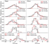 |
Fig. B.1. Distribution of predictor coefficients LD1major on the left panels and LD1minor on the right panels (Nevin et al. 2019) for galaxies with z < 0.075. We mark the decision boundary for LD1major (resp. LD1minor) with black dashed lines at > 1.16 (resp. > 0.42). We show the DPS in red lines and NBCS in black lines. We show all galaxies in the top panels and present LTG, S0, elliptical and merger galaxies in the lower panels respectively. |
Merger rate estimation using LD1major and LD1minor.
LTGs, which are detected at lower redshift in the DPS and the NBCS, build up the largest sub-sample with 254 of the DPS and 392 of the NBCS. We find indeed a higher major-merger rate of 32% for the DPS in comparison to the NBCS with 25%, whereas we find a slightly lower minor-merger rate for the DPS of 19% in comparison to 21% for the NBCS. For S0 galaxies, we find a higher major (16%) and minor (12%) merger rate for the DPS in comparison to the NBCS (4% and 1% respectively).
In our merger scenario for double-peak emission line galaxies (see Sect. 6), we do not find the expected merger rates using the LDA-method. This may be explained by DPS galaxies being past the coalescence phase, while the method developed by Nevin et al. (2019) is not sensitive to faded and later stages of mergers.
Appendix C: Characteristic parameter distributions
As discussed in Sect. 4.2, we detect higher SFRs inside the SDSS fibre for the DPS in comparison to the NBCS. We find comparable total SFRs and about the same stellar mass distribution. As discussed in Sect. 4.1, we detect more extinction for the DPS in comparison to the NBCS with an excess of about 0.25 mag in the V band. We furthermore find comparable stellar ages for the DPS and the NBCS, comparable time scales and about the same stellar and gas metallicities.
With respect to the morphological classifications, we detect significant differences between the DPS and the NBCS in two subsamples, namely Sb-d and elliptical galaxies. Sb-d galaxies of the DPS show higher mean stellar masses (∼0.2 dex in log(M*/M⊙)) and extinction (∼0.3 mag in V) than Sb-d galaxies of the NBCS (Fig. C.1). Furthermore, we detect a significant excess of SF in the centre of DP Sb-d galaxies. We detect  for Sb-d of the DPS and
  for the NBCS. In the case of elliptical galaxies, we detect a 4 times higher SFR in the DPS in comparison to their NBCS counterpart (Fig. C.1). This is consistent with the fact that elliptical DP galaxies are situated in the main star forming sequence, whereas elliptical galaxies of the NBCS are associated with the quenched red sequence (see Sect. 4.2). Assuming a single stellar population, we find that elliptical galaxies with a DP have on average a 3 Gyr younger stellar population in comparison with those showing a single peak. Similarly, assuming an exponential declining star formation history, we detect two times larger time scales for DP elliptical galaxies.
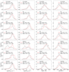 |
Fig. C.1. Each column presents distributions of different parameters of the DPS (red) and the NBCS (black). We show different morphological classifications in each row: in the top row the full samples, followed by Sa, Sb-d, S0s, elliptical, merger and galaxies without classification (see Sect. 3.2). From left to right: first column: star formation rate inside the 3″ SDSS fibre (SFRfibre), second column: total star formation rate (SFRTotal) (Brinchmann et al. 2004), third column: stellar mass M* (Kauffmann et al. 2003). last column: extinction computed with the Balmer decrements Hα/Hβ (Domínguez et al. 2013). We use the non-parametric emission line fit to estimate emission line fluxes taken from Chilingarian et al. (2017). We display the mean and the standard deviation for each distribution. |
Appendix D: Additional material
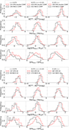 |
Fig. D.1. Comparison of absolute r-band magnitude, Petrosian radii and (SFRfibre) and (SFRtotal) as in Fig. 13, but with DP galaxies classified as COMP in both peak components (red) and galaxies of the NBCS classified as COMP (black) in the upper panels and galaxies classified as S0s in the lower panel. |
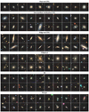 |
Fig. D.2. 62″ × 62″ Legacy Survey snapshots (Dey et al. 2019) of 20 random galaxies of each morphological type, described in Sect. 3.2 (all 10 are shown for Face-on LTGs). |
Fraction of cross match for different BPT and morphological types.
Fraction of cross match for different BPT and morphological types.
Galaxy environment.
All Tables
Comparison of our DPS to other similar works with respect to the selection procedure of this work.
All Figures
|
Fig. 1. Emission lines of three DP galaxies, namely Hβλ4863, [OIII]λ5008, [OI]λ6302, [NII]λ 6550, Hαλ6565, [NII]λ 6585, [SII]λ6718 and [SII]λ 6733. For each panel, we display on the top left, the 62″ × 62″ SDSS snapshot. Each displayed line is fitted with a double Gaussian function as explained in Sect. 2.2. We show the blueshifted Gaussian component as blue lines and the redshifted component as red lines. The green line is a superposition of the two Gaussian components. Below each emission line we show residuals. We flag lines with a confirmed DP selected with criteria described in Sect. 2.2 as “with DP” and flag the others as “no DP” for failing the criteria. The black dashed vertical line indicates the position of the stellar velocity of the host galaxy, computed by Chilingarian et al. (2017). The top spectra are for a face-on spiral galaxy at a redshift of z = 0.02 with a ΔvDP = 232 km s−1, which resembles an outflow (discussed in Sect. 5.6). The middle spectra are for an elliptical galaxy at z = 0.05 showing a ΔvDP = 495 km s−1. The bottom spectra are for a galaxy merger at z = 0.05 and ΔvDP = 269 km s−1. This is one of 58 galaxies discussed in Maschmann & Melchior (2019) showing a DP structure probably associated with recent galaxy merger. |
| In the text | |
|
Fig. 2. Flowchart describing the first two stages of the automated selection procedure, detailed in Sect. 2.2. We list up all selection criteria and note the number of galaxies at each selection step. In stage 1 we select preliminary candidates and a control sample (CS) using emission line properties and χ2 ratios from emission line fitting computed by Chilingarian et al. (2017). We visualise the stacking and fitting procedure and all selection criteria described in Sect. 2.2.2. In stage 2 we describe the individual fitting of each emission line and list up all criteria for the DP flag detailed in Sect. 2.2.4. We finally select 7479 DP candidates and 89 412 galaxies for the CS. |
| In the text | |
|
Fig. 3. Stage 3 of the selection procedure to find the final DPS. This algorithm sorts the fitted emission lines according to their S/N and uses the DP flags indicating confirmed DP in the specific line. All selected galaxies must have a confirmed DP in the strongest line. If the object has more than 1 (resp. 2) confirmed line(s), we must also find a DP in the second (resp. second and third) strongest line. This procedure excludes objects which have a falsely confirmed DP in some weaker lines. We finally get the DPS counting 5663 galaxies. In Table 1, we present the distribution of DP galaxies for different number of confirmed DP. |
| In the text | |
|
Fig. 4. Characteristics of the galaxies selected with a DP feature in their emission lines. From left to right: first panel: flux ratio ϕmax/ϕmin of the stronger line divided by the weaker line for the individual emission lines Hαλ6565, [OIII]λ5008, Hβλ4863 and [NII]λ6585. We display the Hαλ6565 and [OIII]λ5008 emission line ratios of the objects found in Maschmann & Melchior (2019) with blue and re hatched surfaces. The other panels display parameters computed on the stacked spectra (see Sect. 2.2.2). Second panel: velocity difference Δv between the two peak components taken from the stacking procedure. Third (resp. fourth) panel: amplitude (resp. velocity dispersion) ratio of the stronger and weaker line components of the stacked spectra. |
| In the text | |
|
Fig. 5. Stellar mass-redshift distribution for the CS (blue, top left panel) and the DPS (red, top middle panel). The contours indicate the density level. In the top right panel, we show the histogram of stellar masses and, on the bottom left panel, the histogram of redshifts. We also display the fibre diameter corresponding to 3″ on top of the upper left and middle panels. |
| In the text | |
|
Fig. 6. Stellar mass-redshift distribution (see Fig. 5) for the DPS (red) and the NBCS (black). The selection of the NBCS is explained in Sect. 2.3. We also compute histograms for the redshift and the stellar mass for both samples for a better comparison. The NBCS follows the same distribution as the DPS and contains 5128 galaxies. |
| In the text | |
|
Fig. 7. BPT diagrams used to classify our samples into different galaxy types (Kewley et al. 2006b). The red line separates active galactic nuclei (AGN) and composite galaxies (COMP) (Kewley et al. 2001). AGNs and low ionisation narrow emission line regions (LINER) are separated by the green line (Schawinski et al. 2007) and the blue dashed lines separate star forming (SF) and COMP (Kewley et al. 2006b). We present the CS in the upper left panel and the NBCS in the lower left panel. In the upper middle (resp. right) panel, we show the blueshifted (resp. redshifted) peaks of DP galaxies with a S/N > 3 in the four emission line fluxes needed for the BPT diagram. In the lower middle and right panels, we display those emission line components of the DPS with three of the requested emission lines with S/N > 3 and the fourth S/N < 3. To classify them, we display arrows to indicate the limits derived by the uncertainties of weak emission lines. In all six panels, we apply the same colour-coding indicating the specific star formation rate (SSFR) computed by Salim et al. (2016). We display in all panels the same contour lines corresponding to the density of the CS. The corresponding classifications are presented in Table 4. |
| In the text | |
|
Fig. 8. Redshift distribution of the DPS for LTG, S0, merger, and elliptical galaxies. We unified the histogram surface of all four samples to 1. |
| In the text | |
|
Fig. 9. Fraction of different morphological types for the DPs and the NBCS. The error-bars represent the binomial errors. |
| In the text | |
|
Fig. 10. Different parameters distributions of the DPS (red), the CS (blue) and the NBCS (black). The surfaces of all histograms are normalised to unity. In the upper left panel, we compute the absolute AB magnitude in the r-band with Galactic dust and K-corrections estimated by Chilingarian et al. (2017). The lower left panel shows the specific star formation ratio (SSFR) computed by Brinchmann et al. (2004). The middle upper (resp. lower) panel presents the absolute luminosity of the [OIII]λ5008 (resp. Hαλ6565) emission line. The absolute luminosity is calculated using the flux of the non-parametric emission line fit provided by Chilingarian et al. (2017). The right upper panel computes the age assumed by a single stellar population fit by Chilingarian et al. (2017). The right lower panel shows the stellar metallicity computed by Chilingarian et al. (2017). |
| In the text | |
|
Fig. 11. Colour-colour relation between g − r and NUV − r. We present LTG and elliptical galaxies selected from the RCSED catalogue using Domínguez Sánchez et al. (2018) as blue and red contours and show the DPS (resp. NBCS) as black dots in the top panel (resp. lower panel). We display the best-fitting polynomial surface equation of constant absolute z-band magnitudes with coloured lines (Chilingarian & Zolotukhin 2012). |
| In the text | |
|
Fig. 12. SSFR as a function of stellar mass. The top left panel presents LTG and elliptical galaxies selected from the RCSED catalogue using Domínguez Sánchez et al. (2018) as blue and brown contours. These contours are also shown as a reminder in the other panels. We show contour lines indicating the 50%, 68% and 95% level for different morphological subsamples of the DPS (red) and the NBCS (black). We indicate with blue dashed lines the region of intermediate star formation (−11.8 < log(SSFR/M⊙) < −10.8) (Salim 2014) and display the percentage of the morphological types situated in this zone. |
| In the text | |
|
Fig. 13. Distribution of different observables within the 3″ SDSS fibre. We show in three columns three different ranges of redshift. We present galaxies of the DPS which are classified as double SF in red and galaxies classified as SF of the NBCS in black (see Sect. 3.1) In the top row we show the difference in absolute r-band magnitude of the total galaxy and the 3″ SDSS fibre. The colours are Galactic dust- and k-corrected (Chilingarian et al. 2017). In the second row we present the ratio of the radii comprising 90% and 50% of the Petrosian luminosity (Petrosian 1976) approximating the central brightness in comparison to the total galaxy. We show the star formation ratio of the 3″ SDSS fibre SFRfibre in the third row and the ratio between fibre and total star formation (SFRfibre/SFRtotal ) in the bottom row (Brinchmann et al. 2004). |
| In the text | |
|
Fig. 14. Comparison of absolute r-band magnitude, Petrosian radii and SFRfibre and SFRtotal as in Fig. 13 but with DP galaxies classified as AGN in both peak components (red) and galaxies of the NBCS classified as AGN (black). |
| In the text | |
|
Fig. 15. Velocity dispersion distributions for the CS (blue), the NBCS (black) and the DPS (red, purple and orange). The left panel displays the stellar velocity dispersion σ* computed from Chilingarian et al. (2017). The second panel shows the gas velocity dispersion σgas. We compute the Gaussian emission line dispersion for the CS and the NBCS from (Chilingarian et al. 2017). For the DPS, we display the σ1, 2 of the emission line components, which is closer to the galaxy stellar velocity in units of σ1, 2 in magenta and the component which is more offset in cyan. For better comparisons, we unify the surface of the histograms of the left (resp. right) panel to 150 (resp. 100). |
| In the text | |
|
Fig. 16. Single Gaussian approximation. We compute the two Gaussian functions resulting from the double Gaussian fit procedure to the stacked emission line in Sect. 2.2. The blueshifted component is represented by a blue and the redshifted by a red line. In orange, we show the best fit of a single Gaussian function. |
| In the text | |
|
Fig. 17. Comparison of the stellar velocity distribution σ* computed by Chilingarian et al. (2017) with the gas velocity distribution σgas for the NBCS and the velocity distribution of the single Gaussian approximation σsingle for the DPS. We show in red (resp. black) points the median and the 68% quantile for a binning according to σ* of the DPS (resp. NBCS). For the DPS, the limitations in σ1, 2 and ΔvDP of the double Gaussian fit are restricted by the spectral resolution (see Sect. 2.2.2), leading to a restriction of a minimal σsingle, indicated with a red line. We also show the minimal σgas for the NBCS as a black line and the best fit of a linear function as a black dashed line. |
| In the text | |
|
Fig. 18. Influence of the inclination on the velocity dispersion. We show different velocity dispersion distributions as a function of the galaxy inclination for different groups of redshift. We only show LTG and S0 galaxies for which we can compute the inclination using Meert et al. (2015). For the DPS, we show ΔV with red dots, σsingle of the single Gaussian approximation in blue (see Sect. 4.3.2) and in magenta (resp. cyan) the σ of the emission line component which is closer (resp. offset) to the stellar velocity in units of σ. We show the σgas for the NBCS with black dots. All data points represent the medians in the inclination intervals and the error bars the 16th to 84th percentiles. |
| In the text | |
|
Fig. 19. Tully-Fisher relation (TFR) for LTGs. We compute the rotational gas velocity vrot for the NBCS and CS (black and blue contour lines) using the gas velocity dispersion σgas (see Sect. 4.3.1). For the DPS, we use the σsingle of the single Gaussian approximation in the top panel. In the second panel, we show the TFR for the close and far peak-components of the DPS (see Sect. 4.3.1). The stellar masses are computed by Kauffmann et al. (2003). We show the best fit computed by Avila-Reese et al. (2008) as a dashed line. |
| In the text | |
|
Fig. 20. Same as Fig. 19, but for S0 galaxies. The dashed line corresponds to the best fit of Avila-Reese et al. (2008). |
| In the text | |
|
Fig. 21. Faber-Jackson relation for elliptical and S0 galaxies using the stellar velocity dispersion taken from Chilingarian et al. (2017) on the x-axis and the stellar masses computed by Kauffmann et al. (2003) on the y-axis. We show the best fit computed by Gallazzi et al. (2006) in dashed lines. |
| In the text | |
|
Fig. 22. Gini vs M20 coefficients for the DPS (top panel) and the NBCS (lower panel). Blue (resp. orange) contours represent galaxies classified as LTG (resp. S0) and red (resp. green) dots denote elliptical (resp. merger) galaxies (See the classification in Sect. 3.2). The purple line separates galaxies classified as merger on the left hand side and galaxies associated with a Hubble type on the right hand side (Lotz et al. 2004). The lower black dashed line divides elliptical, S0 and Sa galaxies from later types namely Sb, Sc and Irr (Lotz et al. 2008). |
| In the text | |
|
Fig. 23. Distribution of Sérsic indices, computed by STATMORPH (Rodriguez-Gomez et al. 2019) for the Legacy survey r-band images (Dey et al. 2019), of LTGs of the DPS (red line) and NBCS (black line). The areas under the histograms are normalised to unity. |
| In the text | |
|
Fig. B.1. Distribution of predictor coefficients LD1major on the left panels and LD1minor on the right panels (Nevin et al. 2019) for galaxies with z < 0.075. We mark the decision boundary for LD1major (resp. LD1minor) with black dashed lines at > 1.16 (resp. > 0.42). We show the DPS in red lines and NBCS in black lines. We show all galaxies in the top panels and present LTG, S0, elliptical and merger galaxies in the lower panels respectively. |
| In the text | |
|
Fig. C.1. Each column presents distributions of different parameters of the DPS (red) and the NBCS (black). We show different morphological classifications in each row: in the top row the full samples, followed by Sa, Sb-d, S0s, elliptical, merger and galaxies without classification (see Sect. 3.2). From left to right: first column: star formation rate inside the 3″ SDSS fibre (SFRfibre), second column: total star formation rate (SFRTotal) (Brinchmann et al. 2004), third column: stellar mass M* (Kauffmann et al. 2003). last column: extinction computed with the Balmer decrements Hα/Hβ (Domínguez et al. 2013). We use the non-parametric emission line fit to estimate emission line fluxes taken from Chilingarian et al. (2017). We display the mean and the standard deviation for each distribution. |
| In the text | |
|
Fig. D.1. Comparison of absolute r-band magnitude, Petrosian radii and (SFRfibre) and (SFRtotal) as in Fig. 13, but with DP galaxies classified as COMP in both peak components (red) and galaxies of the NBCS classified as COMP (black) in the upper panels and galaxies classified as S0s in the lower panel. |
| In the text | |
|
Fig. D.2. 62″ × 62″ Legacy Survey snapshots (Dey et al. 2019) of 20 random galaxies of each morphological type, described in Sect. 3.2 (all 10 are shown for Face-on LTGs). |
| In the text | |
Current usage metrics show cumulative count of Article Views (full-text article views including HTML views, PDF and ePub downloads, according to the available data) and Abstracts Views on Vision4Press platform.
Data correspond to usage on the plateform after 2015. The current usage metrics is available 48-96 hours after online publication and is updated daily on week days.
Initial download of the metrics may take a while.