| Issue |
A&A
Volume 664, August 2022
|
|
|---|---|---|
| Article Number | A125 | |
| Number of page(s) | 31 | |
| Section | Extragalactic astronomy | |
| DOI | https://doi.org/10.1051/0004-6361/202142218 | |
| Published online | 15 August 2022 | |
Central star formation in double-peak, gas-rich radio galaxies
1
Sorbonne Université, LERMA, Observatoire de Paris, PSL University, CNRS, 75014 Paris, France
e-mail: This email address is being protected from spambots. You need JavaScript enabled to view it.
, This email address is being protected from spambots. You need JavaScript enabled to view it.
2
Collège de France, 11 Place Marcelin Berthelot, 75005 Paris, France
3
Université de Strasbourg, CNRS, Observatoire Astronomique de Strasbourg, UMR 7550, 67000 Strasbourg, France
4
Thüringer Landessternwarte, Sternwarte 5, 07778 Tautenburg, Germany
Received:
14
September
2021
Accepted:
11
May
2022
Abstract
The respective contributions of gas accretion, galaxy interactions, and mergers to the mass assembly of galaxies, as well as the evolution of their molecular gas and star-formation activity are still not fully understood. In a recent work, a large sample of double-peak (DP) emission-line galaxies have been identified from the SDSS. While the two peaks could represent two kinematic components, they may be linked to the large bulges that their host galaxies tend to have. Star-forming DP galaxies display a central star-formation enhancement and have been discussed as compatible with a sequence of recent minor mergers. In order to probe merger-induced star-formation mechanisms, we conducted observations of the molecular-gas content of 35 star-forming DP galaxies in the upper part of the main sequence (MS) of star formation (SF) with the IRAM 30 m telescope. Including similar galaxies 0.3 dex above the MS and with existing molecular-gas observations from the literature, we finally obtained a sample of 52 such galaxies. We succeeded in fitting the same kinematic parameters to the optical ionised- and molecular-gas emission lines for ten (19%) galaxies. We find a central star-formation enhancement resulting most likely from a galaxy merger or galaxy interaction, which is indicated by an excess of gas extinction found in the centre. This SF is traced by radio continuum emissions at 150 MHz, 1.4 GHz, and 3 GHz, all three of which are linearly correlated in log with the CO luminosity with the same slope. The 52 DP galaxies are found to have a significantly larger amount of molecular gas and longer depletion times, and hence a lower star-formation efficiency, than the expected values at their distance of the MS. The large bulges in these galaxies might be stabilising the gas, hence reducing the SF efficiency. This is consistent with a scenario of minor mergers increasing the mass of bulges and driving gas to the centre. We also excluded the inwards-directed gas migration and central star-formation enhancement as the origin of a bar morphology. Hence, these 52 DP galaxies could be the result of recent minor mergers that funnelled molecular gas towards their centre, triggering SF, but with moderate efficiency.
Key words: galaxies: evolution / galaxies: kinematics and dynamics / galaxies: interactions / galaxies: star formation / methods: observational / techniques: spectroscopic
© D. Maschmann et al. 2022
 Open Access article, published by EDP Sciences, under the terms of the Creative Commons Attribution License (https://creativecommons.org/licenses/by/4.0), which permits unrestricted use, distribution, and reproduction in any medium, provided the original work is properly cited.
This article is published in open access under the Subscribe-to-Open model. This email address is being protected from spambots. You need JavaScript enabled to view it. to support open access publication.
1. Introduction
The evolutionary state of galaxies depends mostly on their growth rate and their efficiency when it comes to transforming gas into stars. Galaxy interactions, smooth accretion of gas, and internal mechanisms such as active galactic nucleus (AGN) feedback all affect the gas content and the SF. Galaxy interactions and mergers are well known to enhance the star-formation rate (SFR) (Bothun & Dressler 1986; Pimbblet et al. 2002). However, while they tend to increase the molecular-gas content (Combes et al. 1994; Violino et al. 2018; Lisenfeld et al. 2019), their effect on the evolution of the neutral hydrogen gas fraction is still an open question. Some studies find little difference in close galaxy pairs (e.g. Zuo et al. 2018; Braine & Combes 1993) or post-merger galaxies (e.g. Ellison et al. 2015) compared to the general population of similar galaxies. Other studies find an enhancement of the atomic gas fraction in recently merged galaxies (Huchtmeier et al. 2008; Ellison et al. 2018) or a deficit in the final stages of merging (Hibbard & van Gorkom 1996). The environment can be also responsible for the final quenching of a galaxy (Balogh et al. 1998). Interactions and mergers can also drive gas towards the centre and hence fuel a nuclear black hole, enhancing AGN activity and feedback (Croton et al. 2006; Springel et al. 2005), which can then influence star formation (SF) in the host galaxy (Barrows et al. 2017; Concas et al. 2017; Woo et al. 2017). In cases of powerful AGNs, the radiation can shut down the SF entirely (Di Matteo et al. 2005; Croton et al. 2006; Cattaneo et al. 2009). Relying on simulations, Sanchez et al. (2021) discussed the fact that two successive minor merger events can quench Milky Way-like galaxies through AGN feedback. Based on the projected distances between galaxies and projected velocities, Ellison et al. (2008) and Patton et al. (2011) conducted studies on large galaxy pairs samples and the associated effects. They found an increase of central SF with decreasing galaxy separation. By extending the pair search with quasi stellar objects and AGNs, Ellison et al. (2011a) found that AGN activity can be triggered by galaxy interactions before the final coalescence.
To explain the overall growth of galaxies over cosmic time, Tacchella et al. (2016a) described a scenario of recurring episodes of gas in-fall and depletion phases. Gas is accreted into a galaxy in large amounts through streams from the surroundings (Dekel et al. 2009) or through minor merger events, causing a contraction of the gas disc with efficient star-formation sites and a central enhancement (Dekel & Burkert 2014). This shifts the galaxy above the star-forming main sequence (MS), before gas depletion allows the galaxy to descend underneath the MS. Smooth gas accretion from filaments (Bouché et al. 2010; Davé et al. 2011, 2012; Feldmann 2013; Lilly et al. 2013; Dekel et al. 2013; Peng & Maiolino 2014; Dekel & Burkert 2014) can explain that most galaxies on the MS exhibit a disc morphology (Förster Schreiber et al. 2006; Genzel et al. 2006, 2008; Stark et al. 2008; Daddi et al. 2010; Wuyts et al. 2011) and that star-forming galaxies at z = 1−2 experience long, sustained star-formation cycles (Daddi et al. 2005, 2007; Caputi et al. 2006).
The occurrence of double-peak (DP) emission lines in spectra of galaxies can have different causes, amongst which are galaxy mergers. As predicted by Begelman et al. (1980), galaxy mergers lead at one point to the final coalescence of the supermassive black holes of their progenitors. Earlier stages of this scenario have been reported many times in the form of a dual AGN (e.g. Genzel et al. 2001; Koss et al. 2016, 2018; Goulding et al. 2019). Such galaxy mergers can be identified through kinematic signatures with spectroscopic observations. Post-coalescence mergers can create two separated gas populations, which can be observed as DP emission lines. This has been studied in works focusing on AGN (e.g. Comerford et al. 2009, 2013; Liu et al. 2011, 2013; Koss et al. 2012; Fu et al. 2015). DP signatures were found to be related to merging processes in Comerford et al. (2018) and Maschmann & Melchior (2019). In a recent study, Mazzilli Ciraulo et al. (2021) succeeded in resolving two independent kinematic components using integrated field spectroscopy of a DP emission-line galaxy and identified two galaxies in the process of merging, superimposed in a projection along the line of sight.
In order to discuss the nature of DP emission-line galaxies, Maschmann et al. (2020, hereafter M20) developed an automated selection procedure and found 5663 DP galaxies, including non-AGN galaxies. A systematic search for DP emission-line galaxies was also conducted by Ge et al. (2012) and also included non-AGN galaxies such as star-forming or composite galaxies. M20 relied on reduced spectra provided by the value-added Reference Catalogue of Spectral Energy Distributions (RCSED; Chilingarian et al. 2017) and compared them to single-peaked galaxies with the same emission-line signal-to-noise (S/N) properties and redshift and stellar mass distributions. They found that most of the DP galaxies are massive star-forming galaxies characterised by a central enhancement of their SFR. In addition, they exhibit a large bulge with a Sersic index larger than for the single-peaked galaxy comparison sample. While this configuration could result from repetitive minor mergers, as discussed by Bournaud et al. (2007), it could also correspond to a rotating inner structure. However, as discussed in detail in Mazzilli Ciraulo et al. (2021), integrated field spectroscopy is needed to identify two individual gas components and conclusively identify galaxy mergers. In this work, we studied statistical properties of a sub-sample of 52 galaxies with SDSS spectra.
We explored the most extreme part of this DP sample, focusing on DP galaxies located more than 0.3 dex above the MS. We performed new molecular-gas observations at the IRAM 30 m telescope and completed the sample with existing molecular-gas observations from the literature. We studied the relation between the molecular-gas content and the star-formation activity. In order to test possible biases due to dust, we also used the radio continuum emission, extensively studied as a tracer of SF (Condon 1992; Bell 2003; Schmitt et al. 2006; Murphy et al. 2011). We also relied on the kinematics to explore the possible connection between the ionised and molecular gas. We used these combined analyses to probe the relation between galaxy merging and star-formation mechanisms.
This paper is organised as follows. In Sect. 2, the sample is defined with a description of the CO observations performed at the IRAM 30 m telescope and the data selection from the literature. In Sect. 3, we describe the emission-line fitting and the characteristics of the galaxy sample. We analyse the sample in Sect. 4 with different star-formation tracers and calculate the molecular-gas content. We also present the Kennicutt–Schmidt relation and explore the connection between the CO luminosity and radio continuum emission. Lastly, we discuss our results in Sect. 5 and present the conclusion in Sect. 6. A cosmology of Ωm = 0.3, ΩΛ = 0.7 and h = 0.7 is assumed in this work.
2. Data
We focused on a sample of 52 DP galaxies lying more than 0.3 dex above the MS and gather a few comparison galaxy samples. In Sect. 2.1, the 52-galaxy sample is presented. We discuss the M20 selection of 35 galaxies in Sect. 2.1.1, their observation in CO at the IRAM 30 m telescope in Sect. 2.1.2, and the selection of 17 additional galaxies with CO observations available from the literature in Sect. 2.1.3. In Sect. 2.2, different comparison galaxy samples obtained from existing CO and SFR measurements are described. Lastly, in Sect. 2.3, all the galaxies of the different samples are displayed with respect to their distance from the MS as a function of their stellar mass. In Sect. 2.4, the different samples are cross-identified with existing radio-continuum surveys.
2.1. Sample of 52 DP galaxies 0.3 dex above the MS
The main sample of this work consists of M20 DP galaxies lying more than 0.3 dex above the MS, observed during two observing runs with the IRAM 30 m telescope in April and December 2020.
2.1.1. Selection of M20 DP galaxies 0.3 dex above the MS
We computed the SFR of the MS SFRMS = SFR(MS; z, M*), as parametrised by Speagle et al. (2014), at the redshifts z and stellar masses M* for the DP galaxies of M20 and computed their offset from the MS as δMS = SFR/SFRMS using the SFR computed by Brinchmann et al. (2004) and the stellar masses from Kauffmann et al. (2003). The MS is estimated from observations with a typical scatter of δMS ∼ 0.3 dex (e.g. Noeske et al. 2007; Rodighiero et al. 2011; Whitaker et al. 2012; Schreiber et al. 2015). To target galaxies with increased star-formation activity in comparison to the MS, we thus selected galaxies that are located at least δMS = 0.3 dex above the MS. With this criterion, we aimed to focus our work on galaxies with ongoing SF, which can either be recently induced by galaxy interaction or gas accretion (e.g. Bothun & Dressler 1986; Pimbblet et al. 2002) or be the remainder of a faded starburst event (Schawinski et al. 2009; French et al. 2015). We selected 35 DP galaxies, which we observed with the IRAM 30 m telescope. These galaxies correspond to the red dots of Fig. 1, in which the whole parent M20 sample is shown via grey dots.
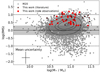 |
Fig. 1. Offset from MS for all CO samples as a function of stellar mass (M*) using the parametrisation of the MS found by Speagle et al. (2014). The shaded area marks the 0.3 dex and the dashed lines the ±1 dex scatter. We used the SFR computed by Brinchmann et al. (2004) and the stellar mass from Kauffmann et al. (2003). We show the M20 sample with grey dots and mark the DP sample (definition in Sect. 2.1) with red circles and stars. Circles represent galaxies with new CO observations and stars represent galaxies for which we obtained the CO measurements from the literature. The contour lines show the density of the M20 sample. In the bottom left, we show the mean uncertainties. |
2.1.2. IRAM-30 m observations of the selected M20 galaxies
We observed the 35 DP galaxies during two observing runs from the 21 to the 24 April 2020 and from the 23 to the 29 December 2020 with the IRAM 30 m telescope at Pico Veleta in Spain. Galaxies with a redshift of z < 0.144 could be observed simultaneously in the CO(1−0) and CO(2−1) lines, and five galaxies at higher redshift were only observable in CO(1−0) at the time. The mean emission-line wavelengths were ∼3 mm for the CO(1−0) line and ∼1.5 mm for the CO(2−1) line. Thick clouds and snow prevented us from observing for 1.5 nights during the first run and two nights during the second run, but we were able to observe all proposed galaxies during the remaining time under excellent conditions.
The galaxies were observed using the broad-band EMIR receiver, tuned in single-band mode with a total bandwidth of 3.715 GHz per polarisation. This allowed us to observe an average velocity range of 11 140 km s−1 for the CO(1−0) line and 5570 km s−1 for the CO(2−1) line. The Wobbler switching mode was used to carry out the observations and the backends WILMA and FTS were used in parallel with a channel width of 2 MHz and 0.195 MHz, respectively.
We pointed, on average, one hour at each galaxy and reached noise levels between 0.1 and 1.8 mK (main-beam temperature), smoothed over 60 km s−1. Focus measurements were performed at the beginning of the night and at dawn, as well as pointing measurements every two hours. The temperature scale we use here is main-beam temperature, and the beam size is λ/D = 22″ at 2.8 mm and 12″ at 1.4 mm wavelength with an average beam efficiency of  and 0.56, respectively. The observation data were reduced using the CLASS/GILDAS software. We transformed the observed main-beam temperature into units of spectral flux density by using the IRAM-30 m-antenna factor of 5 Jy/K, in order to compare our observations with other CO samples.
2.1.3. Inclusion of galaxies with CO data from the literature
In order to enlarge our sample, we further selected DP galaxies lying more than 0.3 dex above the MS from published CO observations. An emission-line fit conducted using the method described in M20 is shown in Fig. 3 for DP-81, one of the 35 galaxies taken from M20. For galaxies from the literature, we performed a simplified DP selection procedure compared to the one of M20, especially with no emission line stacking nor multiple selection stages. Our present algorithm consists of a simultaneous fit of multiple emission lines and selection criteria but we finally rely on a visual inspection, to exclude some noisy spectra but also to enlarge the selection to galaxies with strongly perturbed gas kinematics making emission lines deviate from pure double-Gaussian profiles. The identification of DP emission-line galaxies in literature samples is hence as follows. The best-fitting stellar continuum template provided by Chilingarian et al. (2017) is first subtracted from the SDSS spectrum to obtain the pure emission-line spectrum. Then, we fit single and double-Gaussian functions to the emission lines Hβ, [OIII]λ4960, [OIII]λ5008, [OI]λ6302, [NII]λ6550, Hα, [NII]λ6585, [SII]λ6718, and [SII]λ6733 simultaneously. We also use a global velocity of μ (resp. μ1 and μ2 for the double-Gaussian fit) and a Gaussian standard deviation σ (resp. σ1 and σ2) for all emission lines but keep the individual emission-line amplitudes as free parameters. We also include the spectral instrumental broadening σinst in the fitted σ for each observed emission line individually in order to obtain the observed Gaussian velocity dispersion  . We pre-select galaxies that are selected by the F-test criterion, with an emission-line separation Δv = |μ1 − μ2| of at least 200 km s−1 and an amplitude ratio of the [OIII]λ5008 or Hα line to be between 1/3 and 3, as described in detail in M20.
We select 17 DP galaxies from the literature. These include 11 galaxies observed with the Combined Array for Research in Millimeter-wave Astronomy (CARMA) by Bauermeister et al. (2013), three ultra-luminous infrared galaxies (ULIRG) observed with the 14m telescope of the Five College Radio Astronomy Observatory (FCRAO) observed by Chung et al. (2009), two galaxies observed with the IRAM 30 m telescope as part of the COLD GASS survey (Saintonge et al. 2011, 2017), and one galaxy observed by Solomon et al. (1997), which is known as Arp 220. We found an ALMA-CO(1−0) observation for this galaxy in the ESO archives2. With the high spatial resolution of 37 pc, Scoville et al. (2017) succeeded in precisely locating the two nuclei and studying their nuclear gas discs. We extract the molecular-gas observations from the exact same location as the 3″ SDSS fibre and also from the entire galaxy. We note that the majority of the molecular gas coincides with the two nuclei of Arp 220. However, these two nuclei are strongly obscured by dust, and the SDSS 3″ fibre observation is centred about 4″ north of the two nuclei (Scoville et al. 2017).
We thus gather a DP galaxy sample with CO observations of 52 galaxies lying more than 0.3 dex above the MS: the 35 galaxies from M20 for which we present new CO observations and the 17 galaxies selected from the literature. This sample is presented in Table 1 with characteristic measurements such as the redshift, stellar mass, SFR, radio-continuum fluxes, galaxy size, and inclination. In Sect. 2.2, we further discuss the total DP detection rate for each public CO galaxy sample included in this work.
Characteristics of DP galaxy sample.
2.2. Comparison samples
In order to discuss the peculiarities of our DP sample of 52 galaxies, we assembled complementary galaxy samples from existing CO observations in the literature at different redshifts, star-forming activities, and evolutionary states. For each of these galaxy samples, we performed single and double-Gaussian fits to the SDSS emission-line spectra, when available, as described in Sect. 2.1.3, and present an overview of the DP fractions in Table 2. The DP galaxies lying more than 0.3 dex above the MS have been included in the DP sample of 52 galaxies, as discussed in Sect. 2.1.3.
DP rates in samples from the literature.
2.2.1. Sample from the COLD GASS survey
We use 213 CO(1−0) detected galaxies from the final COLD GASS sample (Saintonge et al. 2011, 2017), observed with the IRAM 30 m telescope with M* greater than M* > 1010 M⊙ and 0.025 < z < 0.050. These constraints exclude the COLD GASS low extension, which is composed of galaxies of 109 M⊙ < M* < 1010 M⊙. We discarded these galaxies since they have an M* of about ∼1−2 dex smaller than the discussed DP sample. Due to their smaller gravitational potential, these galaxies play a different role in terms of merger-induced SF. The selected sample represents the local galaxy population, since it was selected randomly out of the complete parent sample of the SDSS within the ALFALFA footprint. We find 13 galaxies to be identified with a DP and include the two that are situated more than 0.3 dex above the MS in our present DP sample (Sect. 2.1.3).
2.2.2. M sample
To characterise galaxies that are scattered around the MS at higher redshift (z = 0.5−3.2), we composed a CO-detected sample, which is a part of the sample used in Tacconi et al. (2018). This sample is associated with the MS at higher redshift and we name it the M sample. The purpose of this sample is to compare the molecular-gas content and scaling relations of gas depletion time and molecular-gas fractions of DP galaxies with galaxies associated with the MS. We gathered 51 MS galaxies from the PHIBSS1 survey (Tacconi et al. 2013) observed with the IRAM Plateau de Bure Interferometer (PdBI) in CO(3−2) at two redshift groups, z = 1−1.5 and z = 2−2.5, 87 MS galaxies from the PHIBSS2 survey (Tacconi et al. 2018; Freundlich et al. 2019) observed with NOEMA in CO(2−1) or (3−2) at z = 0.5−2.7, nine MS galaxies at z = 0.5−3.2 observed by with IRAM PdBI in CO(2−1) or (3−2) (Daddi et al. 2010; Magdis et al. 2012), six MS galaxies from the Herschel-PACS Evolutionary Probe (PEP) survey (Lutz et al. 2011) observed with the IRAM PdBI in CO(2−1) at redshift z = 1−1.2 (Magnelli et al. 2012), and eight MS gravitationally lensed galaxies observed with the IRAM PdBI in CO(3−2) at z = 1.4−3.2 (Saintonge et al. 2013, and references therein). As shown in Fig. 2, this sample is scattered around the MS with some outliers of up to δMS = 1 dex. Contrary to the sample used in Tacconi et al. (2018), we discuss the COLD GASS sample, the EGNOG and ULIRG samples separately, and exclude all sub-samples of galaxies situated above the MS. We composed the M sample with 161 galaxies. Even though this sample lies at higher redshift than our DP sample, it allows us to discuss underlying mechanisms accounting for deviation from the scaling relations found by Tacconi et al. (2018) and which contribute to various stages of cosmic evolution. Due to their high redshifts, we do not have optical spectra of the M sample galaxies and are thus unable to estimate their DP fraction.
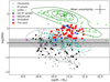 |
Fig. 2. Offset from MS as in Fig. 1. We show the DP sample with red dots, the SP-EGNOG sample with blue dots, the COLD GASS sample with grey dots, the low-SF sample with black dots, the ULIRG sample with green dots, the M sample with turquoise dots, and the MEGAFLOW sample with magenta dots. The literature samples are introduced in Sects. 2.2.1–2.2.6 and a detailed description of the MS is given in Sect. 2.3. We show contour lines for the ULIRG sample in green and for the COLD GASS sample combined with the M sample in grey. In the top right, we show the mean uncertainties of all samples and discuss the individual uncertainties for each sample in the text. |
2.2.3. Sample from the EGNOG survey
We used 31 CO(1−0) or (3−2) galaxies detected above the MS from the EGNOG survey (Bauermeister et al. 2013) at redshift z = 0.06−0.5. These galaxies are mainly characterised by star-formation enhancement and show starbursts in some cases. We have SDSS spectra for 26 of these galaxies and find 11 galaxies exhibiting a DP, which we select in our present DP sample (discussed in Sect. 2.1.3). To discuss the remaining single-peaked (SP) galaxies of this sample, we gather them in the SP-EGNOG sample. The DP galaxies of the EGNOG sample are similar to the present DP sample ones in terms of SFR (Brinchmann et al. 2004), M* (Kauffmann et al. 2003), and redshift. One main difference is the absence of radio continuum observations for the most part of this sample.
2.2.4. ULIRG sample
To compare our galaxies with the brightest infrared (IR) galaxies, we assembled a sample of ultra luminous infrared galaxies (ULIRG) with existing CO detections performed with the IRAM 30 m and the FCRAO 14 m telescope. These galaxies exhibit a starburst or are identified as strong quasars. We selected 18 ULIRGs detected in CO(1−0), (2−1) or (3−2) at z = 0.2−0.6 with far-IR luminosities of log(LFIR/L⊙) > 12.45 (Combes et al. 2011), 15 ULIRGs detected in CO(2−1), (3−2), or (4−3) at z = 0.6−1.0 with log(LFIR/L⊙) > 12 (Combes et al. 2013), 27 ULIRGs detected in CO(1−0) at z = 0.04−0.11 with LFIR = 0.24−1.60 × 10¹² L⊙ (Chung et al. 2009), and 37 CO(1−0) detected ULIRGs at z < 0.3 with LFIR = 0.29−3.80 × 10¹² L⊙ (Solomon et al. 1997). We identify three DP galaxies out of eight SDSS galaxies published by Chung et al. (2009), which are also part of our present sample (defined in Sect. 2.1.3). One DP galaxy out of the eight SDSS galaxies in Solomon et al. (1997) is Arp 220, part of our present DP sample. This provides us 93 ULIRGs, enabling us to compare our DP sample with strong IR and radio sources.
2.2.5. Low-SF sample
To study the difference between star-forming galaxies and galaxies at late stages of a starburst, or even with quenched SF, we gathered a low-SF sample. Therefore, we used 11 galaxies from Schawinski et al. (2009), which were CO(1−0)-detected with the IRAM 30 m telescope. These galaxies are early-type galaxies at a redshift of 0.05 < z < 0.10, currently undergoing the process of quenching or showing late-time SF. We further selected 17 CO(1−0) and (2−1) detected post-starburst galaxies with little ongoing SF (∼1 M⊙ yr−1) at 0.01 < z < 0.12 (French et al. 2015), four of which are exhibiting DP emission lines in the SDSS spectra. We added 15 bulge-dominated, quenched galaxies with large dust lanes detected in CO(1−0) and (2−1) with the IRAM 30 m telescope at 0.025 < z < 0.133 (Davis et al. 2015), three of which have DP emission line in the SDSS spectra. Finally, we added two quenched massive spiral galaxies at z ∼ 0.1 detected in CO(1−0) with the IRAM 30 m telescope (Luo et al. 2020). The low-SF sample therefore consists of 38 galaxies, creating a well-suited counterpart to MS and above-MS galaxies.
2.2.6. MEGAFLOW sample
We aim to discuss our observations with respect to recent NOEMA observations conducted by Freundlich et al. (2021). In a pilot programme of the MusE GAs FLOw and Wind (MEGAFLOW) survey, they measured CO(3−2) and (4−3) detection limits for six galaxies at z = 0.6−1.1 with confirmed inflows and outflows in the circumgalactic medium, to test the quasi-equilibrium model and the compaction scenario describing the evolution of galaxies along the MS, implying a tight relation between SF activity, the gas content, and inflows and outflows. This sample will help us discuss different mechanisms of compaction due to filaments or merger-driven inflows, increasing both the molecular-gas content and the star-formation efficiency, which is discussed in Sect. 5.3.
2.2.7. Fraction of DP galaxies in the comparison samples
Forty-three DP galaxies have been idenfied in the EGNOG, COLD GASS, ULIRG, and low-SF samples. Table 2 shows the fraction of DP galaxies in each sample. The M and the MEGAFLOW samples are not part of the SDSS and it is not possible to derive a DP fraction for them. Furthermore, only 19% of the ULIRG sample is covered by the SDSS, which makes it difficult to estimate a DP fraction. As described in Sect. 2.1.3, only galaxies situated more than 0.3 dex above the MS have been selected for the present DP sample, restricting us to 17 galaxies. Hence, the remaining 26 DP galaxies are excluded from the subsequent analysis of the DP sample.
2.3. Distributions of M* and distance to the MS for all samples
Figure 2 displays the location of the galaxies from all the samples with respect to the MS, as defined in Sect. 2.1. The estimated uncertainty of SFRMS is 0.2 dex (Speagle et al. 2014). We used the SFR estimates provided by Brinchmann et al. (2004) and the M* provided by Kauffmann et al. (2003) for our DP sample, the SF-EGNOG sample, the COLD GASS sample, and the low-SF sample, if available. We estimate a mean uncertainty of 0.1 dex for M* for all these samples. For the SFR measurement, the average uncertainties are 0.3 dex for the DP sample, 0.15 dex for the SF-EGNOG sample, 0.45 dex for the low-SF sample, and 0.4 dex for the COLD GASS sample. The high mean uncertainties for the latter two samples are mainly influenced by quenched galaxies, as they show large SFR uncertainties (Brinchmann et al. 2004). For the M and the MEGAFLOW samples, we used SFR and M* values provided in the literature. An estimate of the mean uncertainties is 0.25 and 0.2 dex for the SFR and M*, respectively (Tacconi et al. 2018; Freundlich et al. 2019, 2021). For the ULIRG sample, we used a literature M* estimate if available and computed the SFR from the LFIR following Kennicutt (1998). The uncertainties for the SFR and M* are 0.2 and 0.15 dex, respectively, as discussed in Genzel et al. (2015). However, many of these galaxies are known to host powerful AGNs, which can contribute substantially to the IR flux. Furthermore, the aperture effects and possible contribution of companions can also lead to a systematic overestimation of both the SFR and the stellar mass (Sanders & Mirabel 1996). Since we cannot quantify systematic uncertainties, we used these estimates with caution.
We find that the M sample, the majority of the COLD GASS sample, the MEGAFLOW sample, and parts of the low-SF sample are situated within the MS. We observe that parts of the COLD GASS and low-SF samples are shifted below the MS. As expected due to their high-IR luminosities, we find the ULIRG sample to be located far above the MS, and in some cases it exceeds 2 dex. Since their SFR is estimated using LFIR, it is possible that in some cases non-stellar gas heating from the AGN dominates the IR emission, biasing the SFR estimate as shown in Ciesla et al. (2015). We find the DP and EGNOG samples situated in the same environment: in the upper MS or above with high stellar masses of ∼1011 M*, and below the ULIRG sample.
2.4. Radio continuum for all samples
To discuss the star-forming activity based on synchrotron emission, we cross-matched the different samples with radio-continuum observation catalogues at 150 MHz, 1.4 GHz, or 3 GHz. These measurements would also be sensitive to the contribution of a possible hidden AGN. We thus selected galaxies observed by the LOFAR Two-metre Sky Survey (LoTSS) at 150 MHz (see Shimwell et al. 2019 for DR1), the Faint Images of the Radio Sky at Twenty-Centimeters (FIRST) at 1.4 GHz (White et al. 1997) or the Very Large Array Sky Survey (VLASS) at 3 GHz (Lacy et al. 2020). We used the integrated radio flux measured for each source. We used the LoTSS DR2 (early access) fluxes as the DR2 offers a larger coverage of SDSS DR7 footprint than the DR1. One can note that the DP galaxies covered by LOFAR observations have been detected.
We include radio measurements at 150 MHz provided by the LoTSS DR2 (see for DR1 Shimwell et al. 2019) and at 3 GHz taken from the VLASS (Lacy et al. 2020). We used the 1.4 GHz observations from the FIRST survey (White et al. 1997) or the NVSS (Condon et al. 1998). In Table 3, we present the fraction of available radio measurements for the different samples. We had early access to the LoTSS DR2, which does not cover the entire northern hemisphere. We thus can only take into account galaxies that are within the observed footprint. We compute the radio luminosity as
 (1)
(1)
Number of available radio measurements for CO samples.
where Fν is the integrated radio-continuum flux at the observed frequency, DL the luminosity distance, and α the spectral index (Condon et al. 2019). We calculated the spectral index using two radio measurements, ν1 and ν2, at two different frequencies:
 (2)
(2)
We preferred to use the radio measurements at 150 MHz and 1.4 GHz if available, otherwise we used a combination with the 3 GHz measurement. For galaxies where we only have a single measurement, we use α = −0.7 (Condon et al. 2019) as an approximation.
3. Data analysis
In Sect. 3.1, we describe the fit applied to the CO emission lines. A combined fit, performed on optical and molecular-gas spectra, enabled us to identify ten DP galaxies with identical kinematic parameters, suggesting a compact molecular-gas configuration. For the remaining galaxies, a single-, a double-, and a triple-Gaussian function are fitted, and the best-fit is selected in order to accurately measure the emission-line integral. In Sect. 3.2, the CO luminosity and the aperture-corrected gas mass are computed. In Sect. 3.3, the characteristics of the DP sample are compared with the literature samples: namely, the BPT diagram, the morphology, and environment and the galaxy inclination. In Sect. 3.4, the SFR measured for the entire galaxy and only the SDSS 3″ fibre are compared.
3.1. CO line fitting
The SDSS 3″ fibre only probes the central few kpc of a galaxy in comparison to the IRAM 30 m CO(1−0) beam of 23″ which covers roughly the entire galaxy at a redshift z > 0.05. So, these two measurements probe not only different types of gas, but also different regions of the galaxy. However, in a scenario where a merger event, a galaxy interaction, or the accretion of a large amount of gas have funnelled the gas into the central region fuelling the SF, we would expect the molecular gas to follow similar kinematics to the ionised gas, with the latter tracing these star-forming regions. Such a scenario would motivate a combined fit approach, where we would expect similar kinematics in the molecular- and ionised-gas measurements.
3.1.1. Combined fit of ionised- and molecular-gas spectra
We tested to see if the same kinematic parameters can be fitted for the ionised-gas and molecular-gas emission lines. Therefore, the same Gaussian kinematic parameters μ1, 2 and σ1, 2 obtained from the optical ionised-gas emission lines (as described in Sect. 2.1.3) are fixed for the CO lines’ fit. Thus, only the emission-line amplitudes are fitted. Then, we checked if the ratios, between the blueshifted and redshifted Gaussian fit components, Ab/AB, for the CO and the Hα emissions are compatible within 3σ. In order to test the significance of the fitted components, we also computed the rms outside the CO emission lines and checked if the residuals of the performed fit exceed three times the rms value. If this is the case, a significant deviation from the residuals would indicate a molecular-gas component that cannot be represented by the velocity distribution found in the ionised gas. In addition, we demanded that each of the two fit components have a signal-to-noise ratio of at least 3. Secondly, if these criteria were met, we adopted this fit and flagged the CO line to indicate a successful combined fit.
When available, we first check the CO(2−1) spectra since this observation probes a smaller region than the CO(1−0) observation. Therefore, if we do not manage to perform a combined fit in the CO(2−1) line, we do not fit the CO(1−0) with this approach. In four galaxies, we only succeeded in fitting a combined fit in the CO(2−1) line and not in the CO(1−0) line. We finally find ten (19%) galaxies with a successful combined fit and show, in Fig. 3, an example of combined fit results with all included lines for DP-8.
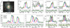 |
Fig. 3. Example of combined emission-line fit for DP-8. We show the Legacy survey snapshot in the top left panel, with a red circle for the SDSS 3″ fibre and dashed green (resp. black) circles for the FWHM of the CO(1−0) (resp. CO(2−1)) beam of the IRAM 30 m telescope. The top row displays, next to the snapshot, the Hβ, [OIII]λ4960, [OIII]λ5008, and [OI]λ6302 emission lines. The bottom row displays the [NII]λ6550, Hα, [NII]λ6585, [SII]λ6718, and [SII]λ6733 emission lines, and two CO emission lines: CO(1−0) and CO(2−1). We show the double-Gaussian fit with the blueshifted (resp. redshifted) component in blue (resp. red) and the total fitted function in green. For each line, we show the residuals below. We display the rms level in yellow for the CO lines, estimated beside the lines. The x-axis measures the deviations from the velocity calculated using the redshift. For the Hα line and the [NII]λ6550, 6585 doublet, we display the lines with respect to the expected Hα line velocity, and, for the [SII]λ6718, 6733, with respect to the [SII]λ6718 line velocity. |
3.1.2. Individual CO emission-line fits
In order to estimate the CO emission lines of those galaxies where the combined fit approach failed, we fitted these spectra individually. To accurately model clumpy line shapes, we fitted each emission line with a single-, a double-, and a triple-Gaussian function and selected the best fit through an F-test, as performed for the ionised-gas emission-line fit in Sect. 2.1.3. This allows us to also model complex line shapes such as a double horn or asymmetric emission lines. To further provide a uniform estimation for the entire DP sample, we performed a single-Gaussian fit for each emission line. This allows us to compare, for example, the full width at half maximum (FWHM) value of each galaxy. In Fig. A.1, we show all results with only the Hα line and the [NII]λ6550, 6585 doublet and the CO lines. We mark a successful combined fit with a flag in each molecular emission line. The CO fit results are presented in Tables B.1 and B.2.
3.2. CO luminosity and H2 mass
To derive the total H2 mass, we first compute the intrinsic CO luminosity with the velocity integrated transition line flux FCO(J → J − 1) and calculate
 (3)
(3)
where νrest is the rest CO line frequency and DL the luminosity distance (Solomon et al. 1997). We can thus derive the total molecular-gas mass including a correction of 36% for interstellar helium using
 (4)
(4)
where the mass-to-light ratio αCO denotes the CO(1−0) luminosity-to-molecular-gas-mass conversion factor, and rJ1 = LCO (J → J − 1)/LCO (1 → 0) is the CO line ratio.
3.2.1. Conversion factor
The conversion factor estimated for the Milky Way and nearby star-forming galaxies with similar stellar metallicities to the Milky Way, including a correction for interstellar helium, is αG = 4.36 ± 0.9 M⊙/(K km s−1 pc2) (Strong & Mattox 1996; Abdo et al. 2010). As discussed in Wolfire et al. (2010) and Bolatto et al. (2013), the CO conversion factor depends on the metallicity. We use a mean value for the correction established by Genzel et al. (2012) and Bolatto et al. (2013) and adopted by Genzel et al. (2015), Tacconi et al. (2018), and Freundlich et al. (2021):
 (5)
(5)
where log Z = 12 + log(O/H) is the gas-phase metallicity on the Pettini & Pagel (2004) scale, which we can estimate from the stellar mass using
 (6)
(6)
with b = 10.4 + 4.46 × log(1 + z)−1.78 × (log(1 + z))2 (see Genzel et al. 2015 and references therein). The gas-phase metallicity can be estimated using optical emission-line ratios, as discussed in Pettini & Pagel (2004). However, the SDSS central 3″ spectral observation is only covering the central part of the galaxy, depending on the redshift. Here, we use Eq. (6) in order to obtain an estimate for the entire galaxy selection and to be consistent with previous works (Genzel et al. 2015; Tacconi et al. 2018; Freundlich et al. 2021). Furthermore, this approach enables us to compute the gas-phase metallicity for galaxies with no available spectral measurements. We find a mean conversion factor for the DP sample of αCO = 3.85 ± 0.08 M⊙/(K km s−1 pc2), which is similar to the conversion factor we find for the EGNOG sample (of 3.86 ± 0.09 M⊙/(K km s−1 pc2)), the low-SF sample (3.86 ± 0.12 M⊙/(K km s−1 pc2)), or the COLD GASS sample (3.84 ± 0.10 M⊙/(K km s−1 pc2)). For the ULIRG sample, we find a slightly higher conversion factor of αCO = 4.00 ± 0.39 M⊙/(K km s−1 pc2). In case we do not have the stellar mass of a galaxy, we use the mean stellar mass of the sample to compute the conversion factor and then the molecular-gas mass. This estimation is adapted for MS galaxies (e.g. Tacconi et al. 2018) and might be overestimated in comparison with the conversion factor of αCO = 0.80 M⊙/(K km s−1 pc2) for ULIRGs discussed in Solomon et al. (1997), and we therefore use this conversion for these galaxies. The molecular-gas mass of the three ULIRGs which we adapted for our DP sample from Chung et al. (2009) are calculated using Eq. (5) in order to keep a consistent molecular-gas-mass estimate.
To compare the calculated molecular-gas masses, we need to assume the line ratio rJ1. In Genzel et al. (2015), Tacconi et al. (2018), and Freundlich et al. (2021), a line ratio of r21 = 0.77 and r31 = 0.5 was assumed, which is used here for the M sample. For the ULIRG sample, we choose ratios of r21 = 0.83, r31 = 0.52, and r41 = 0.42, which are empirically motivated by recent observations (see Genzel et al. 2015 and references therein).
3.2.2. Aperture correction
The closest galaxies that we observed are not entirely covered by the CO(1−0) 22″ beam, resulting in an incomplete measurement of the molecular gas. To account for the gas content outside the telescope beam, we perform an aperture correction following Lisenfeld et al. (2011). Relying on CO maps of local spiral galaxies (Nishiyama et al. 2001; Regan et al. 2001; Leroy et al. 2008), these authors assume an exponential distribution function of the CO gas. Hence, we first define the scale and geometry of each galaxy. To approximate the apparent galaxy size, we extract the optical radius at the 25 mag isophote r25 (see Table 1). As discussed in Lisenfeld et al. (2011), we can assume re/r25 = 0.2 where re is the CO scale length. We measure the galaxy inclination using the minor-to-major axial ratio b/a estimated from a 2D Sérsic profile fit using the photometric diagnostic software STATMORPH3 (Rodriguez-Gomez et al. 2019). We compute the inclination i as
 (7)
(7)
where q0 describes the intrinsic axial ratio of an edge-on observation and is set to q0 = 0.2 (Catinella et al. 2012; Aquino-Ortíz et al. 2018). For galaxies classified as mergers, we set the inclination to 0°, since we cannot identify their orientation with a Sérsic profile. Lastly, following Lisenfeld et al. (2011), the aperture correction factor is computed as
![Mathematical equation: $$ \begin{aligned} {f_{\rm a}} =&\pi r_{\rm e}^{2} \Bigg \{ \int ^{\infty }_{0} \mathrm{d}x \int ^{\infty }_{0} \mathrm{d}y \, \mathrm{exp} \left(-\mathrm{ln}(2) \left[\left( \frac{2 \, x}{ \Theta _{\rm B}}\right)^2 + \left(\frac{2 \,y \, \mathrm{cos}(i)}{ \Theta _{\rm B}}\right)^2\right]\right) \nonumber \\&\times \mathrm{exp} \left(-\frac{\sqrt{x^2 + y^2}}{r_{\rm e}}\right) \Bigg \}^{-1}, \end{aligned} $$](/articles/aa/full_html/2022/08/aa42218-21/aa42218-21-eq10.gif) (8)
(8)
where ΘB is the FWHM of the observation beam. We carry out the integration numerically.
We present the aperture correction factors and the corrected molecular-gas masses in Table B.3. We set the correction factor to 1 for galaxies that are observed using interferometry since we have accurate molecular-gas-mass measurements. We measure a mean correction factor for the DP sample of fa = 1.27. We present the CO luminosities, the molecular-gas mass, and the aperture correction in Table B.3.
3.3. DP sample characteristics
The properties of the DP galaxies are discussed here. These include their position on the BPT diagram (Sect. 3.3.1), their morphology and their environment (Sect. 3.3.2), and their inclination (Sect. 3.3.3).
3.3.1. BPT diagram
We use the BPT diagnostic diagram (Baldwin et al. 1981) to classify our galaxy samples based on optical emission-line ratios: [OIII]λ5008/Hβ on the y-axis and [NII]λ6585/Hα on the x-axis. Relying on the criteria empirically found by Kewley et al. (2006), we differentiate between SF galaxies, AGN, and composite (COMP) galaxies, which are characterised by both mechanisms: SF and AGN. In the top panel of Fig. 4, we show the position on the BPT diagram of the DP, COLD GASS, SP-EGNOG, and low-SF samples. Depending on which function fits the data better, we use the Gaussian or the non-parametric emission-line estimate provided by Chilingarian et al. (2017). For the DP sample, for example, we used the latter, which gives us a global estimation of the entire emission line. In order to characterise each emission-line component individually, we classify each of them separately. We present both classifications in the lower panel of Fig. 4 and list their classifications in Table 4. We also show the classification using the non-parametric fit. In order to unambiguously classify each emission-line component, the Hβ and [OIII]λ5008 lines must be detected, with an S/N > 3, at least, which is not always the case, as for DP-45 and DP-51. However, using the non-parametric fit we are able to classify DP-51.
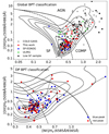 |
Fig. 4. BPT diagrams to classify our galaxy samples into different galaxy types based on ionised-gas emission-line ratios (Kewley et al. 2006). The black solid line separates AGN and COMP galaxies and the dashed black line star-forming galaxies from COMP galaxies. Top panel: galaxies of all samples with existing SDSS spectra. We use Gaussian or non-parametric emission-line fits, in case of a non-Gaussian emission-line shape, provided by Chilingarian et al. (2017). Bottom panel: for each galaxy of the DP sample, the blueshifted and redshifted peaks represented by blue and red squares, respectively, and connect them by a black dashed line. In comparison to the top panel, we zoomed into the region where we detect DP galaxies, to resolve both components. For galaxies with one of the needed emission lines below 3σ, we indicate the emission-line ratio limits with arrows. In both panels, we show contour lines representing galaxies of the RCSED catalogue which have a S/N > 3 in all required emission lines. |
Characteristics of observed galaxies.
Using the non-parametric fit, we classify 56% of the DP sample as SF, 37% as COMP, and 4% as AGNs. The DP sample is dominated by SF galaxies, which is consistent with the fact that the DP sample was selected 0.3 dex above the MS. When each emission-line component is considered individually, nine galaxies (17%) have their two components classified differently. In particular, we find seven SF + COMP, one SF + AGN, and one COMP + AGN. However, we do not find any trend in molecular-gas mass, morphological type, or success of combined fit for these peculiar galaxies.
We classify galaxies of all samples, if possible, with the BPT diagram and build up SF-COMP sub-samples of all galaxies classified as SF or COMP, and an active galaxy sample for those classified as AGNs. For the ULIRG sample, we use classifications provided in the literature since we have SDSS spectra of ten galaxies enabling a detailed BPT classification. We classify all Low Intensity Narrow Emission-line Regions (LINER), Seyfert galaxies, and quasars as an AGN sub-sample. Galaxies of the ULIRG sample show large fractions of strong radio galaxies, we thus do not select any SF-COMP sub-sample for them since we are not able to correctly characterise their AGN contribution. This classification allows us to test the radio flux as a tracer of molecular gas in SF galaxies and to discuss the behaviour of AGN galaxies.
3.3.2. Morphology and galaxy environment
To further characterise the evolutionary state of the galaxies, we visually inspect the legacy survey images (Dey et al. 2019) and categorise them as mergers if we see an optical perturbation, as late-type galaxies (LTG) if we can identify a spiral disc, or as S0 if we can identify a disc with the bulge dominating the shape. The results found by Domínguez Sánchez et al. (2018), using a machine-learning-based classification discussed in M20, inspired this classification.
We also flag LTG and S0 galaxies that have tidal features, since this can be the sign of a recent merger or interaction. In Table 4, we present the morphological type of each galaxy of the DP sample.
We find 27% to be classified as LTG, 38% as S0 galaxies, and 35% as mergers. We also find 13% to be either S0 galaxies or LTG with notable tidal features. A close examination of all DP LTGs reveals that they are all bulge-dominated and Sa types. In order to compare the obtained merger fraction to the one of single-peaked emission-line galaxies, we select 1000 single-peak galaxies from Maschmann et al. (2020) that are situated at 0.3 dex above the MS, and we classify them in the exact same way. This sample of single-peaked emission-line galaxies was selected with the same S/N ratio thresholds of the Hα and O[III]λ5008 emission lines and following the same redshift and stellar mass distribution as the DP galaxy sample of Maschmann et al. (2020). For this galaxy sample, we find only 10% mergers and 14% galaxies with tidal features. It is not straightforward to compare these two galaxy samples. On the one hand, we selected four ULIRGs for the DP sample from the literature, which are all mergers, and on the other hand, galaxies with unusually high SFR values were selected for our CO observations, introducing a bias. However, we find 48% of the DP sample to show either a visual merger or tidal features, which is about twice as much as we find for single-peak emission-line galaxies.
To discuss the fact that we see more bulge-dominated galaxies in the DP sample, we perform a morphological classification of other nearby galaxies samples. Using the Legacy Survey images, we can classify the SP-EGNOG, the COLD GASS, and the low-SF samples in the exact same way as for the DP sample without adding a bias of resolution due to larger redshifts to this classification. The SP-EGNOG sample shows a very similar distribution of stellar masses and SFR as discussed in Sect. 2.3. We also find a very similar morphological composition of 30% LTG, 40% S0, and 10% mergers. The remaining 20% are at redshift 0.5 and thus not classifiable with the Legacy Survey images. Interestingly, we also find the LTG galaxies of the SP-EGNOG sample to be bulge-dominated and Sa type. Furthermore, we detect fewer mergers but identify 25% of the LTG and S0 galaxies to have tidal features. In order to compare the DP sample to the literature galaxies, we classify the galaxies of the COLD GASS sample that are situated more than 0.3 dex above the MS. These galaxies have a mean stellar mass of log(M*/M⊙) = 10.5, which is 0.5 dex smaller than the mean stellar mass of the DP sample. We find 63% of LTGs, 18% of S0 galaxies, and 18% of galaxy mergers. The LTGs exhibit smaller bulges which are of type Sb or Sc. The low-SF sample, in contrast, consists of only 13% LTGs and 18% mergers. However, we find 68% to be classified as bulge-dominated galaxies (i.e. S0 or elliptical galaxies). While the merger rates are not discriminant, the low-SF sample is dominated by early-type galaxies partly quenching explaining their low SFR, while the COLD GASS sample hosts more disc-like galaxies with smaller bulges than the DP sample.
To discuss the impact of the environment, we identify the associated group galaxies using Saulder et al. (2016) for galaxies at z < 0.11, and Yang et al. (2007) for galaxies at z > 0.11. In Saulder et al. (2016), galaxy groups were identified using a group-finding algorithm that was calibrated with cosmological simulations. The group-finding algorithm in Yang et al. (2007) is a halo-based friends-of-friends finding algorithm. Both algorithms provide the number of galaxies in the group and we can measure the projected distance to the closest neighbour. In Table 4, we present the environment parameters for each DP galaxy.
3.3.3. Relation between inclination and kinematics
A rotating disc creating different velocity measurements within the line of sight of a galaxy can create a double-horn or double-peak signature (e.g. Westmeier et al. 2014). In such a scenario, we may expect to see at least a correlation between the galaxy inclination and the FWHM of the CO emission lines. We therefore performed a single-Gaussian fit to the CO emission lines and compare the measured FWHM to the galaxy inclination i, as estimated in Sect. 3.2.2. We use the CO(2−1) line since it has a higher S/N in comparison to the CO(1−0) line in the DP sample. For galaxies with no CO(2−1) observations, we use the CO(1−0) line. The beam sizes of the CO(1−0) and CO(2−1) observations are different (23″ and 12″, respectively) for the 35 galaxies observed at the IRAM-30 m telescope and for the 17 galaxies obtained from the literature, measured with different telescopes and beam sizes. Given the DP galaxies’ redshift distributions, the CO emission lines are not measured on uniform scales. However, as described in Sect. 3.2.2, most measurements include the majority of the molecular gas. The relation between the CO FWHM and the galaxy inclination for the DP sample is displayed in Fig. 5. The mean values and the standard deviation of the CO FWHM for groups of different inclinations are shown. Galaxies classified as mergers are presented separately, since the Sérsic profile fit to the r-band image does not necessarily represent the disc orientation of the galaxies. Inclinations are gathered in three groups: 20° < i < 40°, 40° < i < 60°, and 60° < i < 80°. Galaxies for which we succeeded in applying a combined line fit are indicated as black stars (see Sect. 3.1).
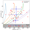 |
Fig. 5. Values of CO FWHM (x-axis) for different galaxy inclinations i (y-axis) of the DP sample. Black stars (resp. red dots) are galaxies for which we succeeded (resp. fail) in applying a combined line fit (see Sect. 3.1). Since it is not possible to measure the inclination of galaxy mergers, we show their FHWM values separately in the grey area at the bottom of the plot. Mean values of the FWHM and standard deviations are displayed with blue error bars for three groups of different inclinations and for the merger sub-sample. The curves show the relation between FWHM and inclination obtained for the estimate of Eq. (9) for a rotating disc, with vrot = 100, 200, 300, and 400 km s−1 for the blue, orange, green, and purple curves, respectively, and with gas velocity dispersions of 10 and 40 km s−1 for solid and dashed lines. |
We are not able to find any trend or correlation between the measured FWHM and the galaxy inclinations. A large scatter is, however, expected even in the case of rotating discs, depending on the mass concentration of the galaxies and also on the velocity dispersion of the molecular gas. A rotation curve rises all the more steeply as mass is concentrated, leading to a dependency of the measured velocities on the mass concentration for a given stellar mass (for typical massive galaxies whose mass is dominated by baryonic matter in their central parts). As the CO gas emission tends to be concentrated, the corresponding velocity measurements may probe only a part of the rising of the rotation curve. A more concentrated stellar bulge will thus likely lead to a larger detected FWHM of the CO emission lines. To illustrate this effect, in Fig. 5 we show a few curves corresponding to different measured rotation velocities, representing measurements for a varying mass concentration at fixed stellar mass, and with two different molecular-gas velocity-dispersion values. We use the simple estimate:
 (9)
(9)
corresponding to the expected width of a double-horn velocity profile widened by a gas-velocity dispersion σ for a disc rotating at vrot with an inclination of i. The first term corresponds to the contribution of the velocity of the gas in the orthogonal direction to the disc plane, and the second term corresponds to the disc’s in-plane gas velocity, dominated by rotation. We also do not find different effects between galaxies with and without a successful combined fit. The rotation velocity of disc galaxies depends on galaxy mass (Tully & Fisher 1977), but by taking their stellar mass into account, we were still not able to detect any trend. These findings are in agreement with results on ionised-gas velocity dispersions and galaxy inclination of a larger DP sample (M20).
3.4. Star formation
To compute the extinction-corrected luminosity of the Hα emission line, we used the following Calzetti (2001):
 (10)
(10)
where Lint(Hα) is the intrinsic and Lobs(Hα) the observed Hα luminosity. κ(Hα) is the reddening curve parametrised by Calzetti et al. (2000) at the Hα rest-frame wavelength, and E(B − V), the colour excess, is computed as
![Mathematical equation: $$ \begin{aligned} {E(B-V) = 1.97\, \log _{10} \left[ \frac{(\mathrm{H}\alpha / \mathrm{H}\beta )_{\rm obs}}{2.86}\right]}, \end{aligned} $$](/articles/aa/full_html/2022/08/aa42218-21/aa42218-21-eq13.gif) (11)
(11)
following Momcheva et al. (2013) and Domínguez et al. (2013). The dust extinction estimate is based on the assumption of an intrinsic Hα/Hβ ratio of 2.86, appropriate for a temperature of T = 104 K and an electron density of ne = 102 cm−3 for a case B recombination (Osterbrock & Ferland 2006). We can thus compute the Hα-based SFR as SFR(Hα) = 7.9 × 10−42 × Lint(Hα) following Kewley et al. (2002).
We compute the SFRHα inside the SDSS 3″ fibre for both emission-line components of the DP sample and the total emission-line luminosity using the non-parametric emission-line fit provided by Chilingarian et al. (2017). To assess the quality of this estimate, we compare the SFRHα estimate to the SFR estimate of the SDSS fibre SFRfibre provided by Brinchmann et al. (2004), which is based on an emission-line modelling to avoid creating biases in the SFR estimated from the emission lines as a function of metallicity or stellar mass. This approach also takes the diffuse emission inside a galaxy into account. In Fig. 6, we show the specific star formation rate sSFR = SFR/M* inside the 3″ fibre using the stellar mass estimate (Kauffmann et al. 2003), considering the SFRHα on the x-axis and the SFRfibre on the y-axis. We present galaxies from the RCSED catalogue with an S/N > 10 in the Hα emission line with black contours and show the mean values of groups of different extinction E(B − V) computed following Eq. (11). We show the DP sample with red dots using the SFR estimate with the non-parametric emission-line fit to account for the entire system. We find the sSFRHα to be underestimated of around 1 dex in comparison with the sSFRfibre for the DP sample. This systematic effect correlates with the measured dust extinction. We observe a mean value of E(B − V) = 0.66 ± 0.19 mag for the DP sample, which is in agreement with the observed offset for SF galaxies of the RCSED with comparable gas-extinction values. Although we corrected the Hα luminosity for extinction, strong dust obscuration can shield parts of the optical light from star-formation sites. This phenomenon was discussed in greater detail in Sanders & Mirabel (1996) and references therein. To calculate the SFR correctly, the estimate of the Hα luminosity has to be combined with IR estimates as performed e.g. in Pancoast et al. (2010). This means that the calculated SFRHα for both components is systematically underestimated but still provides an estimate enabling us to compare the SF contribution of both components.
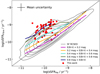 |
Fig. 6. Comparison of sSFR estimate inside the SDSS 3″ fibre. On the x-axis, we show the sSFR estimated from extinction corrected Hα luminosities (SFRHα), and on the y-axis, we show the sSFR inside the fibre (SFRfibre) estimated by Brinchmann et al. (2004). The DP sample is marked with red circles, and the galaxies with an S/N > 10 in the Hα line of the RCSED catalogue (Chilingarian et al. 2017) are marked with black contour lines. We also show the median of groups of different gas extinction E(B − V), computed following Eq. (11), with solid thick lines. The black dashed line denotes SFRHα = SFRfibre. The black error bar is the mean estimated uncertainty of the SFR, including stellar mass uncertainties. |
Besides the SFRfibre, Brinchmann et al. (2004) estimated the SFRtotal for the entire galaxy, enabling us to test if SF is concentrated in the central parts of the galaxy or is equally distributed in the disc. In Fig. 7, we show the ratio of ℛ = SFRfibre/SFRtotal for the DP sample, the EGNOG sample, the COLD GASS sample, and the low-SF sample. We also show subsets of BPT classifications as discussed in Sect. 3.3.1. This diagnostic method is only meaningful for galaxies at lower redshift since the 3″ SDSS fibre covers the entire galaxy at higher redshift. We thus exclude the galaxies of z ∼ 0.5 of the EGNOG sample from this study. We also do not show galaxies of the M sample or the ULIRG sample, since these galaxies have either no SDSS spectral observation or do not show any difference between fibre and total SFR due to their high redshift. We note that the SFRtotal is calculated using star-formation history modelling, which relies on a first estimate of SFRfibre from Brinchmann et al. (2004). This can result in an SFRtotal estimate smaller than the SFRfibre, creating ratios slightly greater than one.
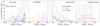 |
Fig. 7. Ratio of SFR inside the 3″ SDSS fibre SFRfibre and the total SFR SFRtotal (Brinchmann et al. 2004). We show this relation for galaxies processed by Brinchmann et al. (2004), which are, from left to right, the DP galaxies, 14 galaxies of the SP-EGNOG survey, 161 galaxies of the COLD GASS sample, and 74 galaxies of the low-SF sample. Subsets of BPT classification of SF are in yellow, those of COMP are in magenta, those of AGNs are in black, and those of the total histogram are in grey. For the DP sample, the subset of galaxies with successful combined fit is indicated with a hatched blue histogram. The scales of the histograms are in arbitrary units. |
For the DP and SP-EGNOG samples, we find a tendency towards a ratio of 1 (ℛDP = 0.81 ± 0.25 and ℛSP − EGNOG = 0.77 ± 0.32, respectively). The galaxies of the DP sample with a successful combined fit (see Sect. 3.1) show an even higher mean ratio of ℛDP = 0.90 ± 0.19, indicating that the majority of their SF is happening in the centre. In contrast to that, we find the opposite effect with no central enhancement of SF for galaxies of the COLD GASS sample (ℛCOLD GASS = 0.27 ± 0.24). The low-SF sample exhibits a very broad distribution (ℛlow SF = 0.48 ± 0.26). Given the measurement uncertainties, we can observe that the DP and the SP-EGNOG samples are clearly biased in favour of large values of ℛ, in particular with respect to the COLD GASS sample.
4. Results
In Sect. 4.1, the ionised- and molecular-gas kinematics measured in single apertures are compared. Section 4.2 is focused on the correlation between the molecular gas and the radio continuum. The position of all samples on the Kennicutt–Schmidt relation are discussed in Sect. 4.3. Lastly, the variation of the molecular-gas fraction and depletion time with redshift and with the relative distance to the MS are studied in Sect. 4.4.
4.1. Kinematical arguments: Mergers, rotating discs, and outflows
Since the measurements of ionised and molecular gas used in this work do not originate from the same area, we compare the FWHM values of the ionised gas and the CO lines in Fig. 8. We show the uncertainties with error bars estimated from the fit. Their size can be in some cases smaller than the marker, which is due to high S/N values.
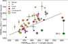 |
Fig. 8. Comparison of FWHMs of ionised- and molecular-gas emission lines, estimated from a single-Gaussian function for the DP sample galaxies. The FWHMs of the ionised-gas emission lines (x-axis) measured inside the 3″ SDSS fibre are estimated by Chilingarian et al. (2017). The FWHMs of the CO line (x-axis) are measured as described in Sect. 3.3.3. The black dashed line denotes y = x. Error bars are estimated from the single-Gaussian line fitting. Stars indicate galaxies classified as mergers. The markers are coloured according to the BPT classification (see Sect. 3.3.1): SF in yellow, COMP in magenta and AGN in black. We mark galaxies for which we succeed in applying a combined line fit (see Sect. 3.1) by red circles. The four ULIRGs of the DP sample are marked with green circles. For the galaxy DP-1, the CO-FWHM is estimated both inside the 3″ SDSS fibre and for the entire galaxy, and the two points are connected with a green dashed line. |
We find that the CO FWHM values are, on average, larger than those of the ionised gas. This can be explained since the CO measurement probes a larger area. For a typical rotation curve rising with radius before reaching a plateau, the widths of the emission lines depend on the part of the rotation curve encompassed by the fibre or beam. If the SDSS fibre encompasses a smaller extent of the rising part of the rotation curve than the CO beam, the ionised emission line is expected to be narrower. The width of the ionised-gas emission lines can, however, be similar to the CO ones, even if the ionised gas extends further away than the SDSS fibre, if the galaxy mass is concentrated enough for the SDSS fibre to encompass the beginning of the plateau of the rotation curve.
In Sect. 3.1, we discuss a combined fit that we performed to select galaxies that show similar kinematics in the ionised and molecular gas. These are highlighted in Fig. 8. The majority of these galaxies are situated near the y = x line, except for two galaxies (DP-20 and DP-33) that have CO FWHM values of about 100 km s−1 larger than the FWHM estimated for the ionised gas. While they met the selection criteria discussed in Sect. 3.1, they give an idea of the expected scatter. In parallel, many galaxies are very close to the y = x line but do not meet the combined fit criteria due to low S/N values and different double peak ratios.
We also observe galaxies with larger FWHM values for the ionised gas than for the molecular gas. This is expected due to ionised-gas outflows driven by a central AGN. As displayed in Fig. 8, most galaxies classified as composite or AGNs are near the y = x line or below. In particular, for DP-1, which is the resolved (ULIRG) galaxy of the DP sample, we observe that the FWHM of the molecular gas inside the 3″ fibre is more than two times smaller than for the optical spectra. When one integrates over the whole galaxy, the molecular gas is still well below the y = x line. Also, the other galaxies lying below the y = x line, including the two of the four ULIRGs marked with green circles, show a broader ionised-gas velocity distribution. This is not expected to be due to rotation, but it is compatible with AGN outflows, which could account for velocities undetected in CO. Interestingly, while mergers are spread all over Fig. 8, the majority of the galaxies below the y = x line are mergers, suggesting a link between the AGN feedback and the merging process. In contrast to that, we find that the majority of the galaxies classified as SF lie above the y = x line, but fewer of these SF galaxies are classified as mergers.
4.2. CO and radio-luminosity correlation
Star-formation sites accelerate electrons and positrons in supernova remnants to high energies, emitting synchrotron radiation when interacting with the galaxies magnetic field (e.g. Condon 1992). It is thus possible to directly trace the SF with radio continuum observations, which is a well-established technique at 1.4 GHz (Condon 1992; Bell 2003; Schmitt et al. 2006; Murphy et al. 2011) and has also proven to be valid at 150 MHz, as shown in Calistro Rivera et al. (2017) and Wang et al. (2019). In contrast, electrons and positrons can also be accelerated in relativistic jets of AGN and shock regions as discussed in, for example, Meisenheimer et al. (1989). In extended radio lobes, these high-energy particles interact with the magnetic-field-creating sychrotron emission (see e.g. Krause et al. 2012). Both mechanisms result in a spectrum described by a power law of S(ν)∝να, where S(ν) is the radio flux and α the spectral index.
SF depends directly on the molecular-gas reservoir, and thus another way to exploit this connection is the relation between the radio luminosity and  . This relation has been known for a long time using the 1.4 GHz radio continuum, and it dates back to the beginning of CO observations (Rickard et al. 1977; Israel & Rowan-Robinson 1984; Murgia et al. 2002). Recently, Orellana-González et al. (2020) quantified this relation as
  = (1.04 ± 0.02) L1.4 GHz − 14.09 ± 0.21 for galaxies at z < 0.27 for more than five orders of magnitude of the luminosities. We aimed to test this relation for the selected CO samples by distinguishing between star-forming galaxies and those with AGN contribution.
In Fig. 9, we show the correlation between  and radio luminosity at 150 MHz, 1.4 GHz, and 3 GHz. The average uncertainties of the observed radio fluxes are 7% at 150 MHz, 5% at 1.4 GHz, and 11% at 3 GHz and are indicated by an error bar. We mark active galaxies with dots, SF galaxies with yellow stars, and COMP galaxies with purple stars. We find a good agreement with the empirical correlation found by Orellana-González et al. (2020) for L1.4 GHz and observe a similar behaviour for the SF-COMP sub-samples at 3 GHz and 150 MHz. We note that galaxies classified as AGNs do not follow such a linear relation. The ULIRG sample especially shows a clear excess in radio luminosity in comparison to other galaxies with comparable
  measurements. This might be an indicator that the radio-continuum emission is dominated by the AGN and is thus no longer correlated with the molecular gas. We fit a straight line to all three relations by only using the SF+COMP sub-samples, and we show the fit results in Table 5. For the
  − L1.4 GHz relations, we find a less steep slope (0.80 ± 0.05) than Orellana-González et al. (2020) (1.04 ± 0.02). However, taking the scatter of 0.32 into account, these two estimates are still comparable. Interestingly, we find similar parameters for the
  − L150 MHz, the
  − L1.4 GHz, and the
  − L3 GHz relations with nearly the exact same slope.
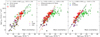 |
Fig. 9. Correlation between |

Fit results of  – radio correlation.
4.3. Kennicutt–Schmidt relation
Figure 10 displays the empirical Kennicutt–Schmidt (KS) relation relating the gas density and SFR through a power law (Schmidt 1959; Kennicutt 1998). On the x-axis, we plot the SFR surface density ΣSFR = SFR/πR2, and on the y-axis we plot the molecular-gas surface density ΣH2 = MH2/πR2, where R is the half-light radius provided in the literature from optical high-resolution images, if available, or computed from a 2D Sérsic profile adjusted to the legacy r-band image as explained in Sect. 3.2.2. In the top panel of Fig. 10, we show the unresolved KS relation. We use the same SFR estimates as used for the MS offset estimate in Sect. 2.3. We plot straight lines of constant depletion times tdepl = MH2/SFR of 0.1, 1, and 10 Gyr. We also mark the MS depletion time of 1.24 Gyr, computed by Tacconi et al. (2018), for the mean redshift (z = 0.10) and stellar mass (log(M*/M⊙) = 11.0) of the DP sample. We display the mean uncertainties with error bars that include an average surface estimation uncertainty of 0.2 dex (van der Wel et al. 2012).
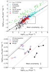 |
Fig. 10. Kennicutt–Schmidt (KS) relation for CO samples. Top panel: KS relation using the total molecular-gas mass and the SFR of the all of the galaxies, and we normalise both quantities using the half-light radii. The DP sample is indicated with red dots, the EGNOG sample with blue dots, the COLD GASS sample with grey dots, the low-SF sample with black dots, the M sample with turquoise dots, and the ULIRG sample with green dots. Galaxies of the low-SF and COLD GASS samples showing AGN activity are marked with stars (see Sect. 3.3.1). Bottom panel: decomposition of the ten DP galaxies for which we succeeded in performing a combined fit (see Sect. 3.1). We show the decomposition in a zoomed-in image of the top panel, which we mark with a dashed box. We display blue (resp. red) squares for the blueshifted (resp. redshifted) component and connect the two components with a black dashed line. We use the SFR estimated by Hα emission of each component and the observed H2 mass of each component and normalise them to the surface of the 3″ SDSS fibre. The three galaxies, classified as mergers, are marked with black plus signs. In both panels, dotted lines denote the constant tdepl of 0.1, 1, and 10 Gyr. The solid black line corresponds to a constant tdepl of 1.24 Gyr estimated using Tacconi et al. (2018) for the mean redshift and stellar mass of the DP sample. In both panels, error bars indicate the mean estimated uncertainties. However, in the lower panel, uncertainties estimated from the surface measurement are not included. |
The DP sample has a mean depletion time of 1.1 ± 0.8 Gyr; for the SP-EGNOG sample, it is 0.7 ± 0.4 Gyr. These are close to the depletion times expected for galaxies situated on the MS. These two samples fill a slight under-density of measurements between the region dominated by nearby galaxies of the COLD GASS sample and the region of the M sample at higher redshifts. The majority of the galaxies of the low-SF sample and the COLD GASS sample follows the same relation as the M sample, but with some galaxies shifted towards lower star-formation efficiencies (with tdepl about 10 Gyr).
We marked galaxies classified as AGNs in Sect. 3.3.1 with stars, and, in fact, the majority of galaxies with very high depletion times are classified as AGNs, which is consistent with a scenario where the AGN is quenching ongoing SF (e.g. Shimizu et al. 2015). Nevertheless, some galaxies with large depletion times do not host any detected AGN activity. This might be due to the exhaustion of their gas reservoir or to a hidden AGN. In contrast, all ULIRGs have significantly smaller depletion times of ∼0.01 Gyr and show the largest range of ΣH2 measurements. Furthermore, as we discussed in Sect. 2.2, their SFR might be overestimated due to AGN contribution, since it was computed using LFIR, shifting the galaxies towards regions of smaller depletion times.
In the bottom panel of Fig. 10, we show the KS relation for the ten DP galaxies with a successful combined fit (see Sect. 3.1). Since we find similar gas distributions between the ionised and the molecular gas, we may assume that the majority of the detected molecular gas (see Sect. 3.1) is situated in the central part of the galaxy, fuelling central SF, as discussed in Sect. 3.4. We show on the y-axis ΣSFR Hα, the SFR surface density estimated using the extinction-corrected Hα luminosity of each peak component (see Sect. 3.4). As discussed in Sect. 3.4, this SFR estimate is systematically underestimated by about 1 dex for the DP sample. On the x-axis, we show the individual H2 mass surface densities ΣH2 fibre, without applying any aperture correction. Both surface densities are calculated for the SDSS 3″ fibre. We also display the mean uncertainties as in the top panel. However, no uncertainties for the surface measurements are included, which leads to significantly smaller error bars. We show the redshifted (resp. blueshifted) peak with a red (resp. blue) square and connect them with a dashed line. The three galaxies, which are classified as mergers, are marked with black plus signs. Interestingly, we find these galaxies to be shifted towards higher molecular-gas surface densities than the non-mergers. As discussed in Sect. 3.4, the SFRHα estimates are most likely underestimated, causing a shift towards larger tdepl as observed in the top panel of Fig. 10. Since the SFRHα is systematically underestimated, we are only able to effectively compare the relative difference in tdepl of the two components.
If an evenly distributed rotating gaseous disc were at the origin of a DP structure, we would expect to observe similar SF efficiencies in each component, comparable tdepl values, and both components being aligned with the lines of constant tdepl in the KS relation. Alternatively, if the DP structure is derived from two different gas populations, two different SF efficiencies would be expected, with two different values of tdepl, and thus the two components would not be aligned with the lines of constant tdepl. We note that due to the logarithmic scale in Fig. 10, tdepl also scales in a logarithmic manner perpendicularly to the lines of constant tdepl. Hence, the difference in tdepl between the two components is expected the largest for the galaxies near the line of tdepl = 10 Gyr and classified as mergers. These galaxies show a difference in tdepl between 0.2 and 0.5 Gyr. In parallel, a difference in tdepl of up to 0.3 Gyr is estimated for the non-merger galaxies.
These trends suggest that the DP signature can probe two different star-formation sites in the merger galaxies, as well as a central disc of homogeneous SF in the LTG and S0 galaxies. However, taking the uncertainties into account, it is difficult to come to solid conclusions regarding these two scenarios. To correctly classify multiple components in a galaxy, observations with optical integral field spectroscopy and spatially resolved measurements of the molecular gas are needed. Such high-resolution observations might also reveal perturbed merger remnants or contracted gaseous discs in the remaining DP galaxies, for which we fail to perform a combined fit.
4.4. Molecular-gas-mass fraction and depletion time
The evolutionary state of a galaxy is strongly dependent on its SFR relying on the molecular-gas reservoir. We thus characterise the CO samples using the molecular-gas-to-stellar-mass ratio (μgas = MH2/M⊙) and the depletion time (tdepl = MH2/SFR). In Fig. 11, we show μgas and tdepl as a function of log(1 + z) for a redshift range of 0 < z < 3. We present the DP sample, the M sample, the COLD GASS sample, the low-SF sample, the SP-EGNOG sample, the ULIRG sample, and the estimated limits for the MEGAFLOW sample and their estimate obtained through stacking. To discuss the different measurements, we make use of the best-fitting unified scaling relations for μgas and tdepl found by Tacconi et al. (2018):
 (12)
(12)
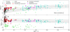 |
Fig. 11. Gas fraction μgas = MH2/M* (top panel) and depletion time tdepl = MH2/SFR (bottom panel) as a function of log(1 + z). We show the observed DP galaxies (red), the EGNOG sample (blue), the COLD GASS sample (grey), the low-SF sample (black), the ULIRG sample (green), the M sample (turquoise), and the detection limits of the MEGAFLOW galaxies (magenta). With an empty circle, we show the estimate based on stacking from Freundlich et al. (2021). The solid black lines represent the scaling relations expected for MS galaxies found by Tacconi et al. (2018), scaled to the mean stellar mass and size of the DP sample (log(M*/M⊙) = 11.0 and Re = 8.3 kpc). The dashed line marks the scatter of 0.4 dex found for the M sample. |
and
 (13)
(13)
where δMS = SFR/SFRMS is the distance to the MS, δM* = M*/5 × 1010 M⊙ is the correction to the fiducial stellar mass of 5 × 10¹⁰ M⊙, and δR = Re/R0, e is the correction of the effective radius Re to the average radius of star-forming galaxies of R0, e = 8.9 kpc(1 + z)−0.75(M*/5 × 1010 M⊙)0.23. In Fig. 11, we show the expected evolution of μgas and tdepl for MS galaxies as a function of redshift and of the mean stellar mass of the DP sample (M* = 1011 M⊙) and the mean size of Re = 8.3 kpc. These relations allow one to visualise how the molecular-gas fraction decreases steeply, since z ∼ 3; whereas, in parallel, the depletion time slightly increases, showing that ongoing SF depends on the available molecular gas. We find that the M sample is still well described by the empirical line and thus presents the scatter of 0.4 dex for the expected scaling relation. We chose this scaling relation since the majority of the literature samples discussed here (COLD GASS, SP-EGNOG, and parts of the ULIRG and the M samples) were used to obtain this relation that is valid over large parts of cosmic time.
Galaxies of the low-SF sample have a large scatter in μgas and in depletion time. Some of these galaxies are quenched due to exhausted gas reservoirs or stopped their SF due to AGN activity. This allows us to probe a wide range of gas fractions and depletion times. Similar behaviour is also observed for the COLD GASS sample. We find that galaxies with long depletion times of these two samples are dominated by AGNs. In contrast, the ULIRG sample shows a large scatter of gas fractions of 1 to 2 dex and very short depletion times of around 0.01 Gyr, which might also be an effect of the overestimation of the SFRs of this sample. As discussed in Sect. 2.3, their stellar mass can be overestimated due to the presence of strong AGNs. While their possibly underestimated mass fraction of gas μgas follows the scaling relation, their depletion time, 2 dex below the scaling relation, is probably underestimated.
The DP and SP-EGNOG samples are shifted above the expected gas fraction, indicating an unusually large gas reservoir, but their depletion time is in the expected range at low redshift. We find two of the DP galaxies (DP-17 and DP-24) to be shifted 2 dex over the expected gas fraction. DP-24 is a ULIRG merger selected from Chung et al. (2009) and DP-17 is a major merger galaxy selected from the COLD GASS sample. We thus assume that the high μgas values are due to an overestimated CO-to-molecular-gas-mass conversion factor (see Sect. 3.2). We also identify three DP galaxies (DP-10, 30, and 44) and one galaxy of the SP-EGNOG (A06) with unexpected small tdepl values of ∼0.1 Gyr. We find all of these galaxies to show a large SFR, between 35 and 106 M⊙ yr−1.
In Fig. 12, we show μgas divided by the expected value provided by Eq. (12) as a function of their relative distance to the MS (δMS) (left panel) and their stellar mass (right panel). We computed the expected SFR value of the MS (SFRMS) following Speagle et al. (2014). In order to compare these values to the expected scaling relations established by Tacconi et al. (2018), we show black lines indicating the relative deviation of μgas from the expected value of the MS μgas(MS). Therefore, we compute μgas, according to Eq. (12), with the fiducial values, despite different δMS (resp. M*) values for the left (resp. right) panel, while the redshift term is cancelled out. We then divide these values by μgas(MS), calculated for the same arbitrary redshift, δMS = 1 and the fiducial values. The resulting function for the left panel is μgas/μgas(MS) = 0.53 log(δMS) and μgas/μgas(MS) = − 0.35 log(δM*) for the right panel. Dashed lines show the scatter found for the M sample.
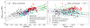 |
Fig. 12. Gas fractions divided by their average values on the MS μgas/μgas(MS) as a function of their relative distance to the MS δMS = SFR/SFRMS (left panel) and stellar mass M* (right panel). We use the predicted μgas(MS) according to Tacconi et al. (2018) and the parametrisation of SFRMS following Speagle et al. (2014). We show the observed DP galaxies (red), the SP-EGNOG sample (blue), the COLD GASS sample (grey), the low-SF sample (black), the ULIRG sample (green), and the M sample (turquoise). For the MEGAFLOW sample, we show the detection limits of each galaxy (magenta) and, with an empty square (resp. star), the estimate reached by stacking for galaxies identified with an outflow (resp. inflow; Freundlich et al. 2021). The solid black lines represent the scaling relations found by Tacconi et al. (2018) and the dashed line marks the scatter of 0.4 dex found for the M sample. |
We present the same samples as for Fig. 11, but for the MEGAFLOW sample we show the stacked estimates for galaxies with identified outflows and inflows separately. As discussed in Freundlich et al. (2021), gas fraction and depletion times are perfectly compatible with the established values of the MS with a mass-selected sample (Tacconi et al. 2018). This indicates that galaxies with identified accretion may not have a specifically high gas content, which is at odds with the theoretical expectations of the quasi-equilibrium and compaction models where the accretion of gas is seen as a gas replenishment. Galaxies from the M sample are scattered around the expected values on the MS; the same is true for the majority of the COLD GASS galaxies. Some galaxies of the COLD GASS and the low-SF samples are shifted below the MS but with significantly large amounts of molecular gas and large tdepl values. As discussed in Sect. 4.3, these outliers are mostly dominated by an AGN. The ULIRG sample exhibits a fraction of molecular gas μgas, which is expected for their distance to the MS according to Tacconi et al. (2018).
Galaxies from the SP-EGNOG sample are slightly shifted above the expected MS μgas values (except A06) but is still compatible with the scatter of the MS. For the DP sample galaxies, due to their selection criteria, they belong to the upper MS. Most of them exhibit a larger molecular-gas reservoir than the MS scaling relation found by Tacconi et al. (2018). As explained above, two galaxies (DP-17 and DP-24) are shifted more than 1 dex above the expected value. In contrast to that, we find three galaxies with smaller gas-mass fractions than expected. Interestingly, these galaxies (DP-10, 30, and 44) are the exact same galaxies that are shifted to significantly shorter tdepl values (see Fig. 11) with strong SFR. This might be an indicator of a late-stage starburst and an almost depleted gas reservoir. For the majority of the DP sample, we see that the expected μgas values are even higher relatively to their shift above the MS. This means, in parallel, that we observe larger tdepl values than we would expect for their distance to the MS. Thus, the gas is not consumed as efficiently as expected, which could be due to recent gas accretion, corresponding to an early-stage starburst. Alternatively, the large bulges characterising the DP galaxies might stabilise the gas and reduce the star-formation efficiency.
In the right panel of Fig. 12, we observe the COLD GASS, low-SF, and M samples to be scattered around the expected values for the MS. However, we observe a strong deviation from the scaling relations for the SP-EGNOG, ULIRG, and DP samples. These samples show larger gas-mass fractions than expected for galaxies of their mass on the MS. The shift above the MS observed for these galaxies might be related to galaxy interactions and mergers that increased their molecular-gas reservoir significantly and fuelled their SF.
5. Discussion
The results are discussed here to account for the properties of the DP sample. Section 5.1 is devoted to galaxies that are mainly star-formation dominated with a remarkable radio-continuum-CO correlation. Section 5.2 discusses the effect of bars. Section 5.3 suggests that DP galaxies are akin to the compaction phase observed after mergers in high-z galaxies.
5.1. Star-formation dominated galaxies
The evolutionary state of galaxies is mostly determined by their growth rate and star-formation efficiency. The relation between SFR and molecular-gas densities is important, since it quantifies the efficiency of the process (see Bigiel et al. 2008 and references therein). In a recent study, Chown et al. (2021) showed that LCO and IR emission at 12 μm describe an even more robust correlation than LCO and SFR. This provides a better estimator to predict the molecular-gas mass for different kinds of galaxies. This is neither significantly affected by the presence of an obscured AGN nor does it rely on a correct choice of the CO-to-H2 conversion factor.
Ongoing SF is also measurable in the IR regime where dust grains are heated from the ultraviolet light emitted by young stars. As discussed in Sect. 4.2, electrons are accelerated in supernova remnants of massive young stars, emitting synchrotron radiation. The underlying process of these two emissions is SF and the radio-continuum-infrared (RC-IR) correlation has been studied extensively for star-forming galaxies (e.g. Bell 2003; Ibar et al. 2008; Ivison et al. 2010; Smith et al. 2014; Liu et al. 2015). Although the RC-IR correlation has long been known as one of the tightest in galaxy physics, Molnár et al. (2021) emphasised the poor match of IR and radio samples that could bias the calibration. They find a slightly non-linear correlation of slope 1.11 ± 0.01.
In order to extend the RC-IR correlation, Orellana-González et al. (2020) found a 3D connection LCO, L1.4 GHz and the infrared luminosity LIR for galaxies with a redshift smaller than z < 0.27. They excluded quasar-like objects to focus on star-formation activity. To further explore this relation, we tested the correlation between LCO and the radio continuum luminosity at 150 MHz, 1.4 GHz, and 3 GHz. We also find a linear relation for galaxies classified as SF or COMP with the BPT diagram (see Sect. 3.3.1) for all three radio-continuum measurements. We performed a linear fit and find a slightly flatter relation between LCO and L1.4 GHz than Orellana-González et al. (2020). Furthermore, we find nearly the same slope for the LCO − L150 MHz relation (0.80 ± 0.06), the LCO − L1.4 GHz relation (0.79 ± 0.04), and the LCO − L3 GHz relation (0.87 ± 0.07).
We also find that these linear relations are not valid for the majority of ULIRGs, which are mostly active galaxies such as quasars or AGNs. Galaxies with high-IR luminosities were observed to be nearly all advanced mergers with circumnuclear-starburst and AGN activity (Sanders & Mirabel 1996). Such galaxies might characterise an important stage of quasar formation and powerful radio galaxies, which is compatible with the large offset that the ULIRG sample shows between CO and radio continuum luminosities. To which relative fractions the ongoing starburst and the AGN are contributing to the IR and radio-continuum luminosities is still under debate (e.g. Dietrich et al. 2018).
Hence, the slope for SF and COMP galaxies measured constant over a wide range of radio wavelengths might be an indicator that the underlying process is dominated by SF. This is also in agreement with DP galaxies having comparable depletion times of around 1 Gyr (see Sect. 4.3). In particular, the good agreement between results at 1.4 GHz, 3 GHz, and 150 MHz suggests that the latter observable is a robust tracer for SF (Calistro Rivera et al. 2017; Wang et al. 2019). Hence, the presented DP sample is dominated by SF with no significant AGN contribution, as confirmed by the BPT classification discussed in Sect. 3.3.1. Indeed, only two galaxies (DP-1 and DP-22), respectively a merger and a S0 galaxy, exhibit AGN excitation on the BPT diagram, but they have a high SFR and high molecular-gas content.
5.2. Gas infall due to bars
Bars are well known to effectively transport gas inwards and create a central starburst. The torques they exert may lead to the creation of star-forming rings in the central parts of galaxies or to the accumulation of gas in the very centre (see Buta & Combes 1996 for a review). Sakamoto et al. (1999) showed, using a sample of nearby galaxies, that the central molecular-gas concentration is higher in barred systems than in unbarred galaxies. This leads to a central star-formation enhancement, which they estimated to be larger than 0.1−1 M⊙ yr−1. By comparing barred, unbarred, and interacting systems, Chown et al. (2019) found that cold gas is transported inwards by a bar or tidal interaction, which leads to the growth and rejuvenation of SF in the central region. Ellison et al. (2011b) found that bars are responsible for 3.5 times more triggered central SF than galaxy-galaxy interactions.
However, in our sample, we only find DP-13 and DP-14 to show a dominant bar. As discussed in Sect. 3.3.2, the present sample is characterised by bulge-dominated systems and mergers. This suggests that the central star-formation enhancement and the higher gas concentration we observe are most likely related to galaxy interactions and mergers, as we discuss in the next section.
5.3. Central star formation and compaction phase
As mentioned in Sect. 1, galaxy interactions and galaxy mergers can trigger SF (Bothun & Dressler 1986; Pimbblet et al. 2002). Relying on larger galaxy samples with 105 SDSS DR4 galaxy pairs, Li et al. (2008) found a clear star-formation enhancement triggered by galaxy interactions. Based on a systematic search for galaxy pairs in the SDSS DR7, Patton et al. (2011) found evidence for a central starburst induced by galaxy interactions. As discussed in Dekel et al. (2009), the merger mechanism forms steady streams enhancing the growth of the central spheroid, leading to earlier Hubble types. This is a different evolution from one of violent mergers that strongly modify the morphology, and it is in agreement with the hierarchical bulge growth described in Bournaud et al. (2007).
We find that 19% of the DP sample galaxies show the same kinematic signature in the molecular and ionised gases, indicating that in these galaxies, most of the molecular gas is located in the very central region of radius 3″. We furthermore observe a central star-formation enhancement for the majority of the DP sample and detect a significant gas reservoir. These findings confirm a compact central star-formation site supporting an effective molecular-gas transportation into the galaxy centre. This scenario is reminiscent of the gas-compaction phase suggested for z = 2−4 galaxies by observations (e.g. Barro et al. 2013, 2017) and simulations (Zolotov et al. 2015; Tacchella et al. 2016a,b) according to which galaxies experience a central enhancement of SF due to gas contraction at their centres, before inside-out depletion and quenching. This model was further described over large scales of cosmic time by Tacchella et al. (2016a), with repetitive compaction and depletion phases shifting galaxies up and down the MS before finally quenching. Since our galaxies are 0.3 dex above the MS, the central SF enhancement and the similar kinematic distribution in the ionised and molecular gas might be a sign of an ongoing compaction phase. In such a scenario, a recent minor merger, a galaxy interaction or a disc instability funnelled gas into the central parts, initiating SF.
In Sect. 4.4, we find that the DP and SP-EGNOG samples have significantly larger molecular-gas fractions (0.8 dex on average) than main-sequence galaxies of the same mass and redshift ranges studied by Tacconi et al. (2018). This discrepancy can be accounted for by a conversion factor of αCO = 0.80 M⊙/(K km s−1 pc2) adopted for ULIRGs by Solomon et al. (1997). We also observe a central star-formation enhancement for the SP-EGNOG sample, which is indeed very similar to the DP sample in terms of stellar mass and redshift. In Fig. 12, we observe both samples to be situated between the population of the M sample and the extreme case of the ULIRG sample. Both samples are found to be situated at the upper MS and above (see Sect. 2.3), but they also show an increased molecular-gas-mass fraction with only a slight decrease in depletion time. The galaxies of the MEGAFLOW sample, which are galaxies showing inflows and outflows in the circumgalactic medium, are maintaining their SF as described in the quasi-equilibrium model (Freundlich et al. 2021). These galaxies have SFEs compatible with star-formation efficiencies measured for the MS. The offset of the DP sample, observed in Fig. 12, suggests that large amounts of gas were recently accreted, possibly through a merger event, and were effectively funnelled into the central regions, where we observe the majority of the ongoing SF.
6. Conclusions
We present new observations of the molecular-gas content for 35 DP emission-line galaxies with ongoing SF situated more than 0.3 dex above the MS. We considered, in addition, 17 DP galaxies from existing CO samples matching the same criterion, leading to a sample of 52 galaxies. We tried to fit the same double-Gaussian parameters to the central optical emission lines and to the CO lines integrated over the entire galaxy. We succeeded in finding similar kinematic signatures for these two measurements in ten (19%) DP galaxies. By comparing the SFR inside the SDSS fibre and in the total galaxy, we find a significant central enhancement of SF for this DP sample. We discuss the possibility of a rotating gaseous disc creating a DP signature. By comparing the emission-line width of the CO gas and the galaxy inclination, we do not find any correlation; however, considering the scatter expected due to galaxy mass concentration or molecular-gas velocity dispersion, the lack of correlation does not allow us to exclude this origin for the observed DP. A deep gravitational potential can in fact be the origin of the DP. This might be the result of a recent minor merger event or galaxy-galaxy interaction that funnelled gas into the central regions. The DP signature might also be the result of cold gas accretion from cosmic filaments, which recently fell into the galaxy centre. These scenarios account for the observed increase of molecular gas and its funnelling into the central region where the majority of the stars are formed. This is also in agreement with the observed excess of dust extinction in the centre.
Such a recently ignited SF is traced by radio-continuum emission at 150 MHz, 1.4 GHz, and 3 GHz all three of which are linearly correlated in log with  with the same slope. This is a signature of synchrotron emission, mostly dominated by SF. Within this interpretation, the possible merger-induced central SF is happening without a simultaneous increase in AGN activity.
Arguments are discussed concerning whether the observed central SF and the large molecular-gas reservoir are the results of a recent merger. Bar structures in galaxies can also effectively migrate gas inwards, which cannot be the case for the presented galaxy samples as it lacks these morphological types. However, we cannot exclude the possibility that we observe gas-rich spiral galaxies with a central molecular disc formed due to large-scale instabilities. In such a scenario, we would observe a central rotating disc that might not be aligned with the host galaxy’s orientation. To further probe our findings and to distinguish between rotating-disc and merger-induced central SF, high resolution observations of the molecular and ionised gas would be necessary. A kinematic decomposition of spatially extended gas would enable us to further characterise the dynamics of these systems and draw conclusions on the origin of double-peak emission-line galaxies. In addition, we could also explore spatially resolved SF and compare its efficiency with findings for regular spiral galaxies (Bigiel et al. 2008; Leroy et al. 2008) in order to conclude on the underlying process of SF and galaxy growth.
We note that the continuum of the [OI]λ6302 line shows a small dip. This is most likely due to the fact that, for the stellar continuum fit, the emission lines are masked and structures close to the emission lines cannot be accurately modelled. Since we fit all emission lines simultaneously with the same kinematic parameters, this has no effect on the emission-line fit.
Acknowledgments
We thank the anonymous referee who helped us to improve our emission line fitting procedure which finally strengthened the arguments in our analysis and discussion. We thank Susanne Maschmann for helpful advise on the English language. This work is based on observations carried out under the two project numbers 198-19 and 166-20 with the IRAM 30 m telescope at Pico Veleta in Spain. IRAM is supported by INSU/CNRS (France), MPG (Germany) and IGN (Spain). This paper makes use of the following ALMA data: ADS/JAO.ALMA#2015:1:00113:S.ALMA is a partnership of ESO (representing its member states), NSF (USA) and NINS (Japan), together with NRC (Canada), MOST and ASIAA (Taiwan), and KASI (Republic of Korea), in cooperation with the Republic of Chile. The Joint ALMA Observatory is operated by ESO, AUI/NRAO and NAOJ. Funding for the Sloan Digital Sky Survey IV has been provided by the Alfred P. Sloan Foundation, the US Department of Energy Office of Science, and the Participating Institutions. SDSS-IV acknowledges support and resources from the Center for High-Performance Computing at the University of Utah. The SDSS website is www.sdss.org. SDSS-IV is managed by the Astrophysical Research Consortium for the Participating Institutions of the SDSS Collaboration including the Brazilian Participation Group, the Carnegie Institution for Science, Carnegie Mellon University, the Chilean Participation Group, the French Participation Group, Harvard-Smithsonian Center for Astrophysics, Instituto de Astrofísica de Canarias, The Johns Hopkins University, Kavli Institute for the Physics and Mathematics of the Universe (IPMU)/University of Tokyo, the Korean Participation Group, Lawrence Berkeley National Laboratory, Leibniz Institut für Astrophysik Potsdam (AIP), Max-Planck-Institut für Astronomie (MPIA Heidelberg), Max-Planck-Institut für Astrophysik (MPA Garching), Max-Planck-Institut für Extraterrestrische Physik (MPE), National Astronomical Observatories of China, New Mexico State University, New York University, University of Notre Dame, Observatário Nacional/MCTI, The Ohio State University, Pennsylvania State University, Shanghai Astronomical Observatory, United Kingdom Participation Group, Universidad Nacional Autónoma de México, University of Arizona, University of Colorado Boulder, University of Oxford, University of Portsmouth, University of Utah, University of Virginia, University of Washington, University of Wisconsin, Vanderbilt University, and Yale University. The Legacy Surveys (http://legacysurvey.org) consist of three individual and complementary projects: the Dark Energy Camera Legacy Survey (DECaLS; NOAO Proposal ID # 2014B-0404; PIs: David Schlegel and Arjun Dey), the Beijing-Arizona Sky Survey (BASS; NOAO Proposal ID # 2015A-0801; PIs: Zhou Xu and Xiaohui Fan), and the Mayall z-band Legacy Survey (MzLS; NOAO Proposal ID # 2016A-0453; PI: Arjun Dey). DECaLS, BASS and MzLS together include data obtained, respectively, at the Blanco telescope, Cerro Tololo Inter-American Observatory, National Optical Astronomy Observatory (NOAO); the Bok telescope, Steward Observatory, University of Arizona; and the Mayall telescope, Kitt Peak National Observatory, NOAO. The Legacy Surveys project is honoured to be permitted to conduct astronomical research on Iolkam Du‘ag (Kitt Peak), a mountain with particular significance to the Tohono O’odham Nation. LOFAR is the Low Frequency Array designed and constructed by ASTRON. It has observing, data processing, and data storage facilities in several countries, which are owned by various parties (each with their own funding sources), and which are collectively operated by the International LOFAR Telescope (ILT) foundation under a joint scientific policy. The ILT resources have benefited from the following recent major funding sources: CNRS-INSU, Observatoire de Paris and Université d’Orléans, France; BMBF, MIWF-NRW, MPG, Germany; Science Foundation Ireland (SFI), Department of Business, Enterprise and Innovation (DBEI), Ireland; NWO, The Netherlands; The Science and Technology Facilities Council, UK; Ministry of Science and Higher Education, Poland; The Istituto Nazionale di Astrofisica (INAF), Italy. This research made use of the Dutch national e-infrastructure with support of the SURF Cooperative (e-infra 180169) and the LOFAR e-infra group. The Jülich LOFAR Long Term Archive and the German LOFAR network are both coordinated and operated by the Jülich Supercomputing Centre (JSC), and computing resources on the supercomputer JUWELS at JSC were provided by the Gauss Centre for Supercomputing e.V. (grant CHTB00) through the John von Neumann Institute for Computing (NIC). This research made use of the University of Hertfordshire high-performance computing facility and the LOFAR-UK computing facility located at the University of Hertfordshire and supported by STFC [ST/P000096/1], and of the Italian LOFAR IT computing infrastructure supported and operated by INAF, and by the Physics Department of Turin university (under an agreement with Consorzio Interuniversitario per la Fisica Spaziale) at the C3S Supercomputing Centre, Italy.
References
- Abdo, A. A., Ackermann, M., Ajello, M., et al. 2010, ApJ, 710, 133 [Google Scholar]
- Aquino-Ortíz, E., Valenzuela, O., Sánchez, S. F., et al. 2018, MNRAS, 479, 2133 [Google Scholar]
- Baldwin, J. A., Phillips, M. M., & Terlevich, R. 1981, PASP, 93, 5 [Google Scholar]
- Balogh, M. L., Schade, D., Morris, S. L., et al. 1998, ApJ, 504, L75 [NASA ADS] [CrossRef] [Google Scholar]
- Barro, G., Faber, S. M., Pérez-González, P. G., et al. 2013, ApJ, 765, 104 [Google Scholar]
- Barro, G., Faber, S. M., Koo, D. C., et al. 2017, ApJ, 840, 47 [Google Scholar]
- Barrows, R. S., Comerford, J. M., Zakamska, N. L., & Cooper, M. C. 2017, ApJ, 850, 27 [NASA ADS] [CrossRef] [Google Scholar]
- Bauermeister, A., Blitz, L., Bolatto, A., et al. 2013, ApJ, 768, 132 [NASA ADS] [CrossRef] [Google Scholar]
- Begelman, M. C., Blandford, R. D., & Rees, M. J. 1980, Nature, 287, 307 [Google Scholar]
- Bell, E. F. 2003, ApJ, 586, 794 [Google Scholar]
- Bigiel, F., Leroy, A., Walter, F., et al. 2008, AJ, 136, 2846 [NASA ADS] [CrossRef] [Google Scholar]
- Bolatto, A. D., Wolfire, M., & Leroy, A. K. 2013, ARA&A, 51, 207 [CrossRef] [Google Scholar]
- Bothun, G. D., & Dressler, A. 1986, ApJ, 301, 57 [NASA ADS] [CrossRef] [Google Scholar]
- Bouché, N., Dekel, A., Genzel, R., et al. 2010, ApJ, 718, 1001 [Google Scholar]
- Bournaud, F., Jog, C. J., & Combes, F. 2007, A&A, 476, 1179 [NASA ADS] [CrossRef] [EDP Sciences] [Google Scholar]
- Braine, J., & Combes, F. 1993, A&A, 269, 7 [NASA ADS] [Google Scholar]
- Brinchmann, J., Charlot, S., White, S. D. M., et al. 2004, MNRAS, 351, 1151 [Google Scholar]
- Buta, R., & Combes, F. 1996, Fund. Cosm. Phys., 17, 95 [Google Scholar]
- Calistro Rivera, G., Williams, W. L., Hardcastle, M. J., et al. 2017, MNRAS, 469, 3468 [Google Scholar]
- Calzetti, D. 2001, PASP, 113, 1449 [Google Scholar]
- Calzetti, D., Armus, L., Bohlin, R. C., et al. 2000, ApJ, 533, 682 [NASA ADS] [CrossRef] [Google Scholar]
- Caputi, K. I., Dole, H., Lagache, G., et al. 2006, ApJ, 637, 727 [NASA ADS] [CrossRef] [Google Scholar]
- Catinella, B., Kauffmann, G., Schiminovich, D., et al. 2012, MNRAS, 420, 1959 [NASA ADS] [CrossRef] [Google Scholar]
- Cattaneo, A., Faber, S. M., Binney, J., et al. 2009, Nature, 460, 213 [NASA ADS] [CrossRef] [Google Scholar]
- Chilingarian, I. V., Zolotukhin, I. Y., Katkov, I. Y., et al. 2017, ApJS, 228, 14 [NASA ADS] [CrossRef] [Google Scholar]
- Chown, R., Li, C., Athanassoula, E., et al. 2019, MNRAS, 484, 5192 [NASA ADS] [CrossRef] [Google Scholar]
- Chown, R., Li, C., Parker, L., et al. 2021, MNRAS, 500, 1261 [Google Scholar]
- Chung, A., Narayanan, G., Yun, M. S., Heyer, M., & Erickson, N. R. 2009, AJ, 138, 858 [NASA ADS] [CrossRef] [Google Scholar]
- Ciesla, L., Charmandaris, V., Georgakakis, A., et al. 2015, A&A, 576, A10 [NASA ADS] [CrossRef] [EDP Sciences] [Google Scholar]
- Combes, F., Prugniel, P., Rampazzo, R., & Sulentic, J. W. 1994, A&A, 281, 725 [NASA ADS] [Google Scholar]
- Combes, F., García-Burillo, S., Braine, J., et al. 2011, A&A, 528, A124 [NASA ADS] [CrossRef] [EDP Sciences] [Google Scholar]
- Combes, F., García-Burillo, S., Braine, J., et al. 2013, A&A, 550, A41 [NASA ADS] [CrossRef] [EDP Sciences] [Google Scholar]
- Comerford, J. M., Gerke, B. F., Newman, J. A., et al. 2009, ApJ, 698, 956 [Google Scholar]
- Comerford, J. M., Schluns, K., Greene, J. E., & Cool, R. J. 2013, ApJ, 777, 64 [NASA ADS] [CrossRef] [Google Scholar]
- Comerford, J. M., Nevin, R., Stemo, A., et al. 2018, ApJ, 867, 66 [NASA ADS] [CrossRef] [Google Scholar]
- Concas, A., Popesso, P., Brusa, M., et al. 2017, A&A, 606, A36 [NASA ADS] [CrossRef] [EDP Sciences] [Google Scholar]
- Condon, J. J. 1992, ARA&A, 30, 575 [Google Scholar]
- Condon, J. J., Cotton, W. D., Greisen, E. W., et al. 1998, AJ, 115, 1693 [Google Scholar]
- Condon, J. J., Matthews, A. M., & Broderick, J. J. 2019, ApJ, 872, 148 [NASA ADS] [CrossRef] [Google Scholar]
- Croton, D. J., Springel, V., White, S. D. M., et al. 2006, MNRAS, 365, 11 [Google Scholar]
- Daddi, E., Renzini, A., Pirzkal, N., et al. 2005, ApJ, 626, 680 [NASA ADS] [CrossRef] [Google Scholar]
- Daddi, E., Alexander, D. M., Dickinson, M., et al. 2007, ApJ, 670, 173 [NASA ADS] [CrossRef] [Google Scholar]
- Daddi, E., Bournaud, F., Walter, F., et al. 2010, ApJ, 713, 686 [NASA ADS] [CrossRef] [Google Scholar]
- Davé, R., Oppenheimer, B. D., & Finlator, K. 2011, MNRAS, 415, 11 [Google Scholar]
- Davé, R., Finlator, K., & Oppenheimer, B. D. 2012, MNRAS, 421, 98 [Google Scholar]
- Davis, T. A., Rowlands, K., Allison, J. R., et al. 2015, MNRAS, 449, 3503 [NASA ADS] [CrossRef] [Google Scholar]
- Dekel, A., & Burkert, A. 2014, MNRAS, 438, 1870 [Google Scholar]
- Dekel, A., Birnboim, Y., Engel, G., et al. 2009, Nature, 457, 451 [Google Scholar]
- Dekel, A., Zolotov, A., Tweed, D., et al. 2013, MNRAS, 435, 999 [Google Scholar]
- Dey, A., Schlegel, D. J., Lang, D., et al. 2019, AJ, 157, 168 [Google Scholar]
- Dietrich, J., Weiner, A. S., Ashby, M. L. N., et al. 2018, MNRAS, 480, 3562 [NASA ADS] [CrossRef] [Google Scholar]
- Di Matteo, T., Springel, V., & Hernquist, L. 2005, Nature, 433, 604 [NASA ADS] [CrossRef] [Google Scholar]
- Domínguez, A., Siana, B., Henry, A. L., et al. 2013, ApJ, 763, 145 [CrossRef] [Google Scholar]
- Domínguez Sánchez, H., Huertas-Company, M., Bernardi, M., Tuccillo, D., & Fischer, J. L. 2018, MNRAS, 476, 3661 [Google Scholar]
- Ellison, S. L., Patton, D. R., Simard, L., & McConnachie, A. W. 2008, AJ, 135, 1877 [NASA ADS] [CrossRef] [Google Scholar]
- Ellison, S. L., Patton, D. R., Mendel, J. T., & Scudder, J. M. 2011a, MNRAS, 418, 2043 [NASA ADS] [CrossRef] [Google Scholar]
- Ellison, S. L., Nair, P., Patton, D. R., et al. 2011b, MNRAS, 416, 2182 [NASA ADS] [CrossRef] [Google Scholar]
- Ellison, S. L., Fertig, D., Rosenberg, J. L., et al. 2015, MNRAS, 448, 221 [NASA ADS] [CrossRef] [Google Scholar]
- Ellison, S. L., Catinella, B., & Cortese, L. 2018, MNRAS, 478, 3447 [NASA ADS] [CrossRef] [Google Scholar]
- Feldmann, R. 2013, MNRAS, 433, 1910 [NASA ADS] [CrossRef] [Google Scholar]
- Förster Schreiber, N. M., Genzel, R., Lehnert, M. D., et al. 2006, ApJ, 645, 1062 [Google Scholar]
- French, K. D., Yang, Y., Zabludoff, A., et al. 2015, ApJ, 801, 1 [NASA ADS] [CrossRef] [Google Scholar]
- Freundlich, J., Combes, F., Tacconi, L. J., et al. 2019, A&A, 622, A105 [NASA ADS] [CrossRef] [EDP Sciences] [Google Scholar]
- Freundlich, J., Bouché, N. F., Contini, T., et al. 2021, MNRAS, 501, 1900 [NASA ADS] [Google Scholar]
- Fu, H., Myers, A. D., Djorgovski, S. G., et al. 2015, ApJ, 799, 72 [Google Scholar]
- Ge, J.-Q., Hu, C., Wang, J.-M., Bai, J.-M., & Zhang, S. 2012, ApJS, 201, 31 [Google Scholar]
- Genzel, R., Tacconi, L. J., Rigopoulou, D., Lutz, D., & Tecza, M. 2001, ApJ, 563, 527 [NASA ADS] [CrossRef] [Google Scholar]
- Genzel, R., Tacconi, L. J., Eisenhauer, F., et al. 2006, Nature, 442, 786 [Google Scholar]
- Genzel, R., Burkert, A., Bouché, N., et al. 2008, ApJ, 687, 59 [Google Scholar]
- Genzel, R., Tacconi, L. J., Combes, F., et al. 2012, ApJ, 746, 69 [Google Scholar]
- Genzel, R., Tacconi, L. J., Lutz, D., et al. 2015, ApJ, 800, 20 [Google Scholar]
- Goulding, A. D., Pardo, K., Greene, J. E., et al. 2019, ApJ, 879, L21 [NASA ADS] [CrossRef] [Google Scholar]
- Hibbard, J. E., & van Gorkom, J. H. 1996, AJ, 111, 655 [NASA ADS] [CrossRef] [Google Scholar]
- Huchtmeier, W. K., Petrosian, A., Gopal-Krishna, McLean, B., & Kunth, D. 2008, A&A, 492, 367 [NASA ADS] [CrossRef] [EDP Sciences] [Google Scholar]
- Ibar, E., Cirasuolo, M., Ivison, R., et al. 2008, MNRAS, 386, 953 [NASA ADS] [CrossRef] [Google Scholar]
- Israel, F., & Rowan-Robinson, M. 1984, ApJ, 283, 81 [NASA ADS] [CrossRef] [Google Scholar]
- Ivison, R. J., Magnelli, B., Ibar, E., et al. 2010, A&A, 518, L31 [NASA ADS] [CrossRef] [EDP Sciences] [Google Scholar]
- Kauffmann, G., Heckman, T. M., White, S. D. M., et al. 2003, MNRAS, 341, 33 [Google Scholar]
- Kennicutt, R. C., Jr. 1998, ApJ, 498, 541 [Google Scholar]
- Kewley, L. J., Geller, M. J., Jansen, R. A., & Dopita, M. A. 2002, AJ, 124, 3135 [NASA ADS] [CrossRef] [Google Scholar]
- Kewley, L. J., Groves, B., Kauffmann, G., & Heckman, T. 2006, MNRAS, 372, 961 [Google Scholar]
- Koss, M., Mushotzky, R., Treister, E., et al. 2012, ApJ, 746, L22 [Google Scholar]
- Koss, M. J., Glidden, A., Baloković, M., et al. 2016, ApJ, 824, L4 [NASA ADS] [CrossRef] [Google Scholar]
- Koss, M. J., Blecha, L., Bernhard, P., et al. 2018, Nature, 563, 214 [Google Scholar]
- Krause, M., Alexander, P., Riley, J., & Hopton, D. 2012, MNRAS, 427, 3196 [NASA ADS] [CrossRef] [Google Scholar]
- Lacy, M., Baum, S. A., Chandler, C. J., et al. 2020, PASP, 132, 035001 [Google Scholar]
- Leroy, A. K., Walter, F., Brinks, E., et al. 2008, AJ, 136, 2782 [Google Scholar]
- Li, C., Kauffmann, G., Heckman, T. M., Jing, Y. P., & White, S. D. M. 2008, MNRAS, 385, 1903 [NASA ADS] [CrossRef] [Google Scholar]
- Lilly, S. J., Carollo, C. M., Pipino, A., Renzini, A., & Peng, Y. 2013, ApJ, 772, 119 [NASA ADS] [CrossRef] [Google Scholar]
- Lisenfeld, U., Espada, D., Verdes-Montenegro, L., et al. 2011, A&A, 534, A102 [NASA ADS] [CrossRef] [EDP Sciences] [Google Scholar]
- Lisenfeld, U., Xu, C. K., Gao, Y., et al. 2019, A&A, 627, A107 [NASA ADS] [CrossRef] [EDP Sciences] [Google Scholar]
- Liu, X., Shen, Y., Strauss, M. A., & Hao, L. 2011, ApJ, 737, 101 [Google Scholar]
- Liu, X., Civano, F., Shen, Y., et al. 2013, ApJ, 762, 110 [NASA ADS] [CrossRef] [Google Scholar]
- Liu, L., Gao, Y., & Greve, T. R. 2015, ApJ, 805, 31 [Google Scholar]
- Luo, Y., Li, Z., Kang, X., Li, Z., & Wang, P. 2020, MNRAS, 496, L116 [NASA ADS] [CrossRef] [Google Scholar]
- Lutz, D., Poglitsch, A., Altieri, B., et al. 2011, A&A, 532, A90 [NASA ADS] [CrossRef] [EDP Sciences] [Google Scholar]
- Magdis, G. E., Daddi, E., Sargent, M., et al. 2012, ApJ, 758, L9 [NASA ADS] [CrossRef] [Google Scholar]
- Magnelli, B., Saintonge, A., Lutz, D., et al. 2012, A&A, 548, A22 [NASA ADS] [CrossRef] [EDP Sciences] [Google Scholar]
- Maschmann, D., & Melchior, A.-L. 2019, A&A, 627, L3 [NASA ADS] [CrossRef] [EDP Sciences] [Google Scholar]
- Maschmann, D., Melchior, A.-L., Mamon, G. A., Chilingarian, I. V., & Katkov, I. Y. 2020, A&A, 641, A171 [NASA ADS] [CrossRef] [EDP Sciences] [Google Scholar]
- Mazzilli Ciraulo, B., Melchior, A.-L., Maschmann, D., et al. 2021, A&A, 653, A47 [NASA ADS] [CrossRef] [EDP Sciences] [Google Scholar]
- Meisenheimer, K., Roser, H. J., Hiltner, P. R., et al. 1989, A&A, 219, 63 [NASA ADS] [Google Scholar]
- Molnár, D. C., Sargent, M. T., Leslie, S., et al. 2021, MNRAS, 504, 118 [CrossRef] [Google Scholar]
- Momcheva, I. G., Lee, J. C., Ly, C., et al. 2013, AJ, 145, 47 [NASA ADS] [CrossRef] [Google Scholar]
- Murgia, M., Crapsi, A., Moscadelli, L., & Gregorini, L. 2002, A&A, 385, 412 [NASA ADS] [CrossRef] [EDP Sciences] [Google Scholar]
- Murphy, E. J., Condon, J. J., Schinnerer, E., et al. 2011, ApJ, 737, 67 [Google Scholar]
- Nishiyama, K., Nakai, N., & Kuno, N. 2001, PASJ, 53, 757 [NASA ADS] [Google Scholar]
- Noeske, K. G., Weiner, B. J., Faber, S. M., et al. 2007, ApJ, 660, L43 [CrossRef] [Google Scholar]
- Orellana-González, G., Ibar, E., Leiton, R., et al. 2020, MNRAS, 495, 1760 [CrossRef] [Google Scholar]
- Osterbrock, D. E., & Ferland, G. J. 2006, Astrophysics of Gaseous Nebulae and Active Galactic Nuclei (Sausalito: University Science Books) [Google Scholar]
- Pancoast, A., Sajina, A., Lacy, M., Noriega-Crespo, A., & Rho, J. 2010, ApJ, 723, 530 [CrossRef] [Google Scholar]
- Patton, D. R., Ellison, S. L., Simard, L., McConnachie, A. W., & Mendel, J. T. 2011, MNRAS, 412, 591 [NASA ADS] [CrossRef] [Google Scholar]
- Peng, Y.-J., & Maiolino, R. 2014, MNRAS, 443, 3643 [NASA ADS] [CrossRef] [Google Scholar]
- Pettini, M., & Pagel, B. E. J. 2004, MNRAS, 348, L59 [NASA ADS] [CrossRef] [Google Scholar]
- Pimbblet, K. A., Smail, I., Kodama, T., et al. 2002, MNRAS, 331, 333 [NASA ADS] [CrossRef] [Google Scholar]
- Regan, M. W., Thornley, M. D., Helfer, T. T., et al. 2001, ApJ, 561, 218 [CrossRef] [Google Scholar]
- Rickard, L. J., Palmer, P., Morris, M., Turner, B. E., & Zuckerman, B. 1977, ApJ, 213, 673 [NASA ADS] [CrossRef] [Google Scholar]
- Rodighiero, G., Daddi, E., Baronchelli, I., et al. 2011, ApJ, 739, L40 [Google Scholar]
- Rodriguez-Gomez, V., Snyder, G. F., Lotz, J. M., et al. 2019, MNRAS, 483, 4140 [NASA ADS] [CrossRef] [Google Scholar]
- Saintonge, A., Kauffmann, G., Kramer, C., et al. 2011, MNRAS, 415, 32 [NASA ADS] [CrossRef] [Google Scholar]
- Saintonge, A., Lutz, D., Genzel, R., et al. 2013, ApJ, 778, 2 [Google Scholar]
- Saintonge, A., Catinella, B., Tacconi, L. J., et al. 2017, ApJS, 233, 22 [Google Scholar]
- Sakamoto, K., Okumura, S. K., Ishizuki, S., & Scoville, N. Z. 1999, ApJ, 525, 691 [NASA ADS] [CrossRef] [Google Scholar]
- Sanchez, N. N., Tremmel, M., Werk, J. K., et al. 2021, ApJ, 911, 116 [NASA ADS] [CrossRef] [Google Scholar]
- Sanders, D. B., & Mirabel, I. F. 1996, ARA&A, 34, 749 [Google Scholar]
- Saulder, C., van Kampen, E., Chilingarian, I. V., Mieske, S., & Zeilinger, W. W. 2016, A&A, 596, A14 [NASA ADS] [CrossRef] [EDP Sciences] [Google Scholar]
- Schawinski, K., Lintott, C. J., Thomas, D., et al. 2009, ApJ, 690, 1672 [CrossRef] [Google Scholar]
- Schmidt, M. 1959, ApJ, 129, 243 [NASA ADS] [CrossRef] [Google Scholar]
- Schmitt, H. R., Calzetti, D., Armus, L., et al. 2006, ApJ, 643, 173 [NASA ADS] [CrossRef] [Google Scholar]
- Schreiber, C., Pannella, M., Elbaz, D., et al. 2015, A&A, 575, A74 [NASA ADS] [CrossRef] [EDP Sciences] [Google Scholar]
- Scoville, N., Murchikova, L., Walter, F., et al. 2017, ApJ, 836, 66 [Google Scholar]
- Shimizu, T. T., Mushotzky, R. F., Meléndez, M., Koss, M., & Rosario, D. J. 2015, MNRAS, 452, 1841 [NASA ADS] [CrossRef] [Google Scholar]
- Shimwell, T. W., Tasse, C., Hardcastle, M. J., et al. 2019, A&A, 622, A1 [NASA ADS] [CrossRef] [EDP Sciences] [Google Scholar]
- Smith, D. J. B., Jarvis, M. J., Hardcastle, M. J., et al. 2014, MNRAS, 445, 2232 [Google Scholar]
- Solomon, P. M., Downes, D., Radford, S. J. E., & Barrett, J. W. 1997, ApJ, 478, 144 [NASA ADS] [CrossRef] [Google Scholar]
- Speagle, J. S., Steinhardt, C. L., Capak, P. L., & Silverman, J. D. 2014, ApJS, 214, 15 [Google Scholar]
- Springel, V., Di Matteo, T., & Hernquist, L. 2005, MNRAS, 361, 776 [Google Scholar]
- Stark, D. P., Swinbank, A. M., Ellis, R. S., et al. 2008, Nature, 455, 775 [NASA ADS] [CrossRef] [Google Scholar]
- Strong, A. W., & Mattox, J. R. 1996, A&A, 308, L21 [NASA ADS] [Google Scholar]
- Tacchella, S., Dekel, A., Carollo, C. M., et al. 2016a, MNRAS, 457, 2790 [Google Scholar]
- Tacchella, S., Dekel, A., Carollo, C. M., et al. 2016b, MNRAS, 458, 242 [NASA ADS] [CrossRef] [Google Scholar]
- Tacconi, L. J., Neri, R., Genzel, R., et al. 2013, ApJ, 768, 74 [NASA ADS] [CrossRef] [Google Scholar]
- Tacconi, L. J., Genzel, R., Saintonge, A., et al. 2018, ApJ, 853, 179 [Google Scholar]
- Tully, R. B., & Fisher, J. R. 1977, A&A, 54, 661 [NASA ADS] [Google Scholar]
- van der Wel, A., Bell, E. F., Häussler, B., et al. 2012, ApJS, 203, 24 [NASA ADS] [CrossRef] [Google Scholar]
- Violino, G., Ellison, S. L., Sargent, M., et al. 2018, MNRAS, 476, 2591 [NASA ADS] [CrossRef] [Google Scholar]
- Wang, L., Gao, F., Duncan, K. J., et al. 2019, A&A, 631, A109 [NASA ADS] [CrossRef] [EDP Sciences] [Google Scholar]
- Westmeier, T., Jurek, R., Obreschkow, D., Koribalski, B. S., & Staveley-Smith, L. 2014, MNRAS, 438, 1176 [NASA ADS] [CrossRef] [Google Scholar]
- Whitaker, K. E., van Dokkum, P. G., Brammer, G., & Franx, M. 2012, ApJ, 754, L29 [Google Scholar]
- White, R. L., Becker, R. H., Helfand, D. J., & Gregg, M. D. 1997, ApJ, 475, 479 [Google Scholar]
- Wolfire, M. G., Hollenbach, D., & McKee, C. F. 2010, ApJ, 716, 1191 [Google Scholar]
- Woo, J.-H., Son, D., & Bae, H.-J. 2017, ApJ, 839, 120 [Google Scholar]
- Wuyts, S., Förster Schreiber, N. M., Lutz, D., et al. 2011, ApJ, 738, 106 [Google Scholar]
- Yang, X., Mo, H. J., van den Bosch, F. C., et al. 2007, ApJ, 671, 153 [Google Scholar]
- Zolotov, A., Dekel, A., Mandelker, N., et al. 2015, MNRAS, 450, 2327 [Google Scholar]
- Zuo, P., Xu, C. K., Yun, M. S., et al. 2018, ApJS, 237, 2 [NASA ADS] [CrossRef] [Google Scholar]
Appendix A: Spectra
In Fig. A.1, we show all galaxies of the DP sample. We present their 70″ × 70″ legacy survey snapshot (Dey et al. 2019), the ionised-gas emission lines’ Hα and the [NII]λ6550, 6585 doublet, and the CO spectra. Furthermore, we show the fit results as discussed in Sect. 3.1.
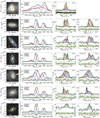 |
Fig. A.1. Fit results of ionised-gas emission lines and CO(1-0)/CO(2-1) lines. On the left, we show the 70″ × 70″ legacy survey snapshots (Dey et al. 2019) and mark the position of the SDSS 3″ fibre in red and the IRAM CO(1-0) (resp. CO(2-1)) beam of 23″ (resp. 12″) with a green (resp. black) dashed line. For interferometry observations conducted by Bauermeister et al. (2013), we show the beam with a blue ellipse. For DP-24, DP-25, and DP-31, we show the FCRAO CO(1-0) beam of 50″. For DP-1, we extracted a CO(1-0) signal from ALMA interferometry observations for the exact same area as the SDSS 3″ fibre. Next to the snapshots, we show the Hα emission line and the [NII]λ6550/6585 doublet fitted with a double-Gaussian function. On the right hand side, we show the CO(1-0) and the CO(2-1) line, if observed, fitted by a single, a double, or a triple-Gaussian function. In the case of a successful combined fit as described in Sect. 3.1, we indicate this in the top left of the CO panels. For a detailed description of the fitting procedure, see Sect. 3.1. |
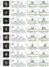 |
Fig. A.1. continued. |
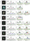 |
Fig. A.1. continued. |
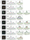 |
Fig. A.1. continued. |
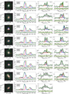 |
Fig. A.1. continued. |
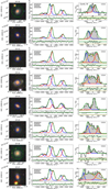 |
Fig. A.1. continued. |
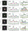 |
Fig. A.1. continued. |
Appendix B: Observation tables
In Table B.1 (resp. B.2), we present the parameters for the CO(1-0) (resp. CO(2-1)) line obtained using our fitting procedure described in Sect. 3.1. In Table B.3, we present the CO-to-MH2 conversion factor, the molecular-gas mass, the aperture correction factor, the estimated molecular-gas-mass fraction, and the depletion time.
Observed CO(1-0) line parameters.
Observed CO(2-1) line parameters.
Results of molecular-gas-mass estimation.
All Tables
All Figures
|
Fig. 1. Offset from MS for all CO samples as a function of stellar mass (M*) using the parametrisation of the MS found by Speagle et al. (2014). The shaded area marks the 0.3 dex and the dashed lines the ±1 dex scatter. We used the SFR computed by Brinchmann et al. (2004) and the stellar mass from Kauffmann et al. (2003). We show the M20 sample with grey dots and mark the DP sample (definition in Sect. 2.1) with red circles and stars. Circles represent galaxies with new CO observations and stars represent galaxies for which we obtained the CO measurements from the literature. The contour lines show the density of the M20 sample. In the bottom left, we show the mean uncertainties. |
| In the text | |
|
Fig. 2. Offset from MS as in Fig. 1. We show the DP sample with red dots, the SP-EGNOG sample with blue dots, the COLD GASS sample with grey dots, the low-SF sample with black dots, the ULIRG sample with green dots, the M sample with turquoise dots, and the MEGAFLOW sample with magenta dots. The literature samples are introduced in Sects. 2.2.1–2.2.6 and a detailed description of the MS is given in Sect. 2.3. We show contour lines for the ULIRG sample in green and for the COLD GASS sample combined with the M sample in grey. In the top right, we show the mean uncertainties of all samples and discuss the individual uncertainties for each sample in the text. |
| In the text | |
|
Fig. 3. Example of combined emission-line fit for DP-8. We show the Legacy survey snapshot in the top left panel, with a red circle for the SDSS 3″ fibre and dashed green (resp. black) circles for the FWHM of the CO(1−0) (resp. CO(2−1)) beam of the IRAM 30 m telescope. The top row displays, next to the snapshot, the Hβ, [OIII]λ4960, [OIII]λ5008, and [OI]λ6302 emission lines. The bottom row displays the [NII]λ6550, Hα, [NII]λ6585, [SII]λ6718, and [SII]λ6733 emission lines, and two CO emission lines: CO(1−0) and CO(2−1). We show the double-Gaussian fit with the blueshifted (resp. redshifted) component in blue (resp. red) and the total fitted function in green. For each line, we show the residuals below. We display the rms level in yellow for the CO lines, estimated beside the lines. The x-axis measures the deviations from the velocity calculated using the redshift. For the Hα line and the [NII]λ6550, 6585 doublet, we display the lines with respect to the expected Hα line velocity, and, for the [SII]λ6718, 6733, with respect to the [SII]λ6718 line velocity. |
| In the text | |
|
Fig. 4. BPT diagrams to classify our galaxy samples into different galaxy types based on ionised-gas emission-line ratios (Kewley et al. 2006). The black solid line separates AGN and COMP galaxies and the dashed black line star-forming galaxies from COMP galaxies. Top panel: galaxies of all samples with existing SDSS spectra. We use Gaussian or non-parametric emission-line fits, in case of a non-Gaussian emission-line shape, provided by Chilingarian et al. (2017). Bottom panel: for each galaxy of the DP sample, the blueshifted and redshifted peaks represented by blue and red squares, respectively, and connect them by a black dashed line. In comparison to the top panel, we zoomed into the region where we detect DP galaxies, to resolve both components. For galaxies with one of the needed emission lines below 3σ, we indicate the emission-line ratio limits with arrows. In both panels, we show contour lines representing galaxies of the RCSED catalogue which have a S/N > 3 in all required emission lines. |
| In the text | |
|
Fig. 5. Values of CO FWHM (x-axis) for different galaxy inclinations i (y-axis) of the DP sample. Black stars (resp. red dots) are galaxies for which we succeeded (resp. fail) in applying a combined line fit (see Sect. 3.1). Since it is not possible to measure the inclination of galaxy mergers, we show their FHWM values separately in the grey area at the bottom of the plot. Mean values of the FWHM and standard deviations are displayed with blue error bars for three groups of different inclinations and for the merger sub-sample. The curves show the relation between FWHM and inclination obtained for the estimate of Eq. (9) for a rotating disc, with vrot = 100, 200, 300, and 400 km s−1 for the blue, orange, green, and purple curves, respectively, and with gas velocity dispersions of 10 and 40 km s−1 for solid and dashed lines. |
| In the text | |
|
Fig. 6. Comparison of sSFR estimate inside the SDSS 3″ fibre. On the x-axis, we show the sSFR estimated from extinction corrected Hα luminosities (SFRHα), and on the y-axis, we show the sSFR inside the fibre (SFRfibre) estimated by Brinchmann et al. (2004). The DP sample is marked with red circles, and the galaxies with an S/N > 10 in the Hα line of the RCSED catalogue (Chilingarian et al. 2017) are marked with black contour lines. We also show the median of groups of different gas extinction E(B − V), computed following Eq. (11), with solid thick lines. The black dashed line denotes SFRHα = SFRfibre. The black error bar is the mean estimated uncertainty of the SFR, including stellar mass uncertainties. |
| In the text | |
|
Fig. 7. Ratio of SFR inside the 3″ SDSS fibre SFRfibre and the total SFR SFRtotal (Brinchmann et al. 2004). We show this relation for galaxies processed by Brinchmann et al. (2004), which are, from left to right, the DP galaxies, 14 galaxies of the SP-EGNOG survey, 161 galaxies of the COLD GASS sample, and 74 galaxies of the low-SF sample. Subsets of BPT classification of SF are in yellow, those of COMP are in magenta, those of AGNs are in black, and those of the total histogram are in grey. For the DP sample, the subset of galaxies with successful combined fit is indicated with a hatched blue histogram. The scales of the histograms are in arbitrary units. |
| In the text | |
|
Fig. 8. Comparison of FWHMs of ionised- and molecular-gas emission lines, estimated from a single-Gaussian function for the DP sample galaxies. The FWHMs of the ionised-gas emission lines (x-axis) measured inside the 3″ SDSS fibre are estimated by Chilingarian et al. (2017). The FWHMs of the CO line (x-axis) are measured as described in Sect. 3.3.3. The black dashed line denotes y = x. Error bars are estimated from the single-Gaussian line fitting. Stars indicate galaxies classified as mergers. The markers are coloured according to the BPT classification (see Sect. 3.3.1): SF in yellow, COMP in magenta and AGN in black. We mark galaxies for which we succeed in applying a combined line fit (see Sect. 3.1) by red circles. The four ULIRGs of the DP sample are marked with green circles. For the galaxy DP-1, the CO-FWHM is estimated both inside the 3″ SDSS fibre and for the entire galaxy, and the two points are connected with a green dashed line. |
| In the text | |
|
Fig. 9. Correlation between |
| In the text | |
|
Fig. 10. Kennicutt–Schmidt (KS) relation for CO samples. Top panel: KS relation using the total molecular-gas mass and the SFR of the all of the galaxies, and we normalise both quantities using the half-light radii. The DP sample is indicated with red dots, the EGNOG sample with blue dots, the COLD GASS sample with grey dots, the low-SF sample with black dots, the M sample with turquoise dots, and the ULIRG sample with green dots. Galaxies of the low-SF and COLD GASS samples showing AGN activity are marked with stars (see Sect. 3.3.1). Bottom panel: decomposition of the ten DP galaxies for which we succeeded in performing a combined fit (see Sect. 3.1). We show the decomposition in a zoomed-in image of the top panel, which we mark with a dashed box. We display blue (resp. red) squares for the blueshifted (resp. redshifted) component and connect the two components with a black dashed line. We use the SFR estimated by Hα emission of each component and the observed H2 mass of each component and normalise them to the surface of the 3″ SDSS fibre. The three galaxies, classified as mergers, are marked with black plus signs. In both panels, dotted lines denote the constant tdepl of 0.1, 1, and 10 Gyr. The solid black line corresponds to a constant tdepl of 1.24 Gyr estimated using Tacconi et al. (2018) for the mean redshift and stellar mass of the DP sample. In both panels, error bars indicate the mean estimated uncertainties. However, in the lower panel, uncertainties estimated from the surface measurement are not included. |
| In the text | |
|
Fig. 11. Gas fraction μgas = MH2/M* (top panel) and depletion time tdepl = MH2/SFR (bottom panel) as a function of log(1 + z). We show the observed DP galaxies (red), the EGNOG sample (blue), the COLD GASS sample (grey), the low-SF sample (black), the ULIRG sample (green), the M sample (turquoise), and the detection limits of the MEGAFLOW galaxies (magenta). With an empty circle, we show the estimate based on stacking from Freundlich et al. (2021). The solid black lines represent the scaling relations expected for MS galaxies found by Tacconi et al. (2018), scaled to the mean stellar mass and size of the DP sample (log(M*/M⊙) = 11.0 and Re = 8.3 kpc). The dashed line marks the scatter of 0.4 dex found for the M sample. |
| In the text | |
|
Fig. 12. Gas fractions divided by their average values on the MS μgas/μgas(MS) as a function of their relative distance to the MS δMS = SFR/SFRMS (left panel) and stellar mass M* (right panel). We use the predicted μgas(MS) according to Tacconi et al. (2018) and the parametrisation of SFRMS following Speagle et al. (2014). We show the observed DP galaxies (red), the SP-EGNOG sample (blue), the COLD GASS sample (grey), the low-SF sample (black), the ULIRG sample (green), and the M sample (turquoise). For the MEGAFLOW sample, we show the detection limits of each galaxy (magenta) and, with an empty square (resp. star), the estimate reached by stacking for galaxies identified with an outflow (resp. inflow; Freundlich et al. 2021). The solid black lines represent the scaling relations found by Tacconi et al. (2018) and the dashed line marks the scatter of 0.4 dex found for the M sample. |
| In the text | |
|
Fig. A.1. Fit results of ionised-gas emission lines and CO(1-0)/CO(2-1) lines. On the left, we show the 70″ × 70″ legacy survey snapshots (Dey et al. 2019) and mark the position of the SDSS 3″ fibre in red and the IRAM CO(1-0) (resp. CO(2-1)) beam of 23″ (resp. 12″) with a green (resp. black) dashed line. For interferometry observations conducted by Bauermeister et al. (2013), we show the beam with a blue ellipse. For DP-24, DP-25, and DP-31, we show the FCRAO CO(1-0) beam of 50″. For DP-1, we extracted a CO(1-0) signal from ALMA interferometry observations for the exact same area as the SDSS 3″ fibre. Next to the snapshots, we show the Hα emission line and the [NII]λ6550/6585 doublet fitted with a double-Gaussian function. On the right hand side, we show the CO(1-0) and the CO(2-1) line, if observed, fitted by a single, a double, or a triple-Gaussian function. In the case of a successful combined fit as described in Sect. 3.1, we indicate this in the top left of the CO panels. For a detailed description of the fitting procedure, see Sect. 3.1. |
| In the text | |
|
Fig. A.1. continued. |
| In the text | |
|
Fig. A.1. continued. |
| In the text | |
|
Fig. A.1. continued. |
| In the text | |
|
Fig. A.1. continued. |
| In the text | |
|
Fig. A.1. continued. |
| In the text | |
|
Fig. A.1. continued. |
| In the text | |
Current usage metrics show cumulative count of Article Views (full-text article views including HTML views, PDF and ePub downloads, according to the available data) and Abstracts Views on Vision4Press platform.
Data correspond to usage on the plateform after 2015. The current usage metrics is available 48-96 hours after online publication and is updated daily on week days.
Initial download of the metrics may take a while.