| Issue |
A&A
Volume 641, September 2020
|
|
|---|---|---|
| Article Number | A18 | |
| Number of page(s) | 23 | |
| Section | Astrophysical processes | |
| DOI | https://doi.org/10.1051/0004-6361/202037531 | |
| Published online | 01 September 2020 | |
Fully compressible simulations of waves and core convection in main-sequence stars
1
Heidelberger Institut für Theoretische Studien, Schloss-Wolfsbrunnenweg 35, 69118 Heidelberg, Germany
e-mail: This email address is being protected from spambots. You need JavaScript enabled to view it.
2
School of Mathematics, Statistics and Physics, Newcastle University, Newcastle upon Tyne NE1 7RU, UK
3
X Computational Physics (XCP) Division and Center for Theoretical Astrophysics (CTA), Los Alamos National Laboratory, Los Alamos, NM 87545, USA
4
Zentrum für Astronomie der Universität Heidelberg, Institut für Theoretische Astrophysik, Philosophenweg 12, 69120 Heidelberg, Germany
5
Instituut voor Sterrenkunde, KU Leuven, Celestijnenlaan 200D, 3001 Leuven, Belgium
6
Department of Astrophysics, IMAPP, Radboud University Nijmegen, PO Box 9010, 6500 GL Nijmegen, The Netherlands
7
Max Planck Institute for Astronomy, Königstuhl 17, 69117 Heidelberg, Germany
Received:
20
January
2020
Accepted:
3
July
2020
Abstract
Context. Recent, nonlinear simulations of wave generation and propagation in full-star models have been carried out in the anelastic approximation using spectral methods. Although it makes long time steps possible, this approach excludes the physics of sound waves completely and requires rather high artificial viscosity and thermal diffusivity for numerical stability. A direct comparison with observations is thus limited.
Aims. We explore the capabilities of our compressible multidimensional Seven-League Hydro (SLH) code to simulate stellar oscillations.
Methods. We compare some fundamental properties of internal gravity and pressure waves in 2D SLH simulations to linear wave theory using two test cases: (1) an interval gravity wave packet in the Boussinesq limit and (2) a realistic 3 M⊙ stellar model with a convective core and a radiative envelope. Oscillation properties of the stellar model are also discussed in the context of observations.
Results. Our tests show that specialized low-Mach techniques are necessary when simulating oscillations in stellar interiors. Basic properties of internal gravity and pressure waves in our simulations are in good agreement with linear wave theory. As compared to anelastic simulations of the same stellar model, we can follow internal gravity waves of much lower frequencies. The temporal frequency spectra of velocity and temperature are flat and compatible with the observed spectra of massive stars.
Conclusion. The low-Mach compressible approach to hydrodynamical simulations of stellar oscillations is promising. Our simulations are less dissipative and require less luminosity boosting than comparable spectral simulations. The fully-compressible approach allows for the coupling of gravity and pressure waves in the outer convective envelopes of evolved stars to be studied in the future.
Key words: hydrodynamics / methods: numerical / stars: interiors / convection / waves
© ESO 2020
1. Introduction
The study of the excitation and propagation of waves within stars has greatly helped to shape stellar structure and evolution theory over the last century. Today, this area of astronomy is called asteroseismology, and it includes the study of oscillations across the Hertzsprung–Russell diagram. For example, pressure modes (p-modes) provide important constraints on the envelopes of stars. Modes of a consecutive radial order (n) and the same angular degree (ℓ) have a characteristic frequency separation known as the large frequency separation, which is sensitive to the average density of a star (Aerts et al. 2010). This application of asteroseismology using p-modes has been extremely successful for low- and intermediate-mass stars (Chaplin & Miglio 2013; Hekker & Christensen-Dalsgaard 2017; García & Ballot 2019). Specifically, the measurement of envelope rotation using rotationally-split pressure modes has facilitated the discovery that stars with masses of about 2 M⊙ have approximately rigid interior rotation profiles (see Kurtz et al. 2014; Saio et al. 2015; Van Reeth et al. 2016, 2018). Hence, current angular momentum theory already needs significant improvement on the main sequence (MS; Aerts et al. 2019).
For later evolutionary stages, including subgiant, red giant, and red clump stars, pulsations that behave as gravity modes (g-modes) near the core and as p-modes near the surface have been detected in thousands of stars (see Beck et al. 2011). These “mixed modes” can be used to distinguish different stages of nuclear burning (Bedding et al. 2011). Hence, understanding pressure modes is not only crucial for measuring interior properties of main sequence stars, but also for post-MS stars (see, e.g., Beck et al. 2012; Mosser et al. 2012).
On the upper main sequence, stars with spectral types O and B (M > 3 M⊙) observed in μmag precision space photometry show coherent opacity-driven p- or g-modes as well as stochastic variability caused by internal gravity waves. This occurs in slowly pulsating B (SPB) stars with masses between 3 M⊙ and 9 M⊙ (Pápics et al. 2017; Bowman et al. 2019a; Pedersen 2020), in β Cep stars with masses between 8 M⊙ and 25 M⊙ (Briquet et al. 2011; Burssens et al. 2019), and in young and evolved O-type dwarfs and blue supergiants with masses up to ∼50 M⊙ (Buysschaert et al. 2015; Bowman et al. 2019b, 2020; Pedersen et al. 2019). This overwhelming observational evidence from CoRoT, Kepler/K2, and TESS photometry motivated the development and study of our simulation setup.
The typical numerical approach to model the excitation of waves generated within stars is to solve the Navier–Stokes equations in the anelastic approximation (e.g., Rogers et al. 2013; Alvan et al. 2014; Edelmann et al. 2019). This method allows for large time steps while still being a mostly explicit method and is therefore computationally efficient. While being suitable to simulate internal gravity waves (IGWs) where gravity is the dominant restoring force, some important phenomena, such as the excitation of p-modes, cannot be followed. Furthermore, common numerical methods to solve the equations in the anelastic approximation require to introduce an artificial viscosity to achieve numerical stability. To balance the effect of high viscosity, the stellar luminosity and the thermal diffusivity have to be increased by orders of magnitude. This leads to a damping of the waves, especially in the low frequency regime.
Some of these drawbacks are avoided or reduced by performing compressible simulations of stellar interiors. Here, the full Navier–Stokes equations are solved, most commonly in the finite volume approach. This includes the physics of sound waves and allows the luminosity and the thermal diffusivity to be kept much closer to stellar values. Viscosity is implicitly introduced by the numerical scheme, and is lower than the viscosity typically used by spectral codes (nevertheless still orders of magnitudes higher than the astrophysical value). This is why we commonly speak of solving the Euler equations, which follow from the Navier–Stokes equations without an explicit viscosity term, in this context. On the other hand, this kind of simulations comes with higher computational costs compared to their anelastic counterparts. That compressible simulations show excited IGWs and p-modes has already been reported in the past. For example, Meakin & Arnett (2006, 2007) show a spectrum of the velocity for a simulation of carbon and oxygen burning in a 3D wedge geometry. They compare the form of a wave with predominately g-mode character and a coupled p- and g-mode to the predictions from linear theory and find good agreement for both. Also Herwig et al. (2006) indicate the excitation of p- and g-modes for the case of He-shell burning. They find the frequency of the different modes to be independent of resolution and boosting.
These prior studies focus on the effects of convective boundary mixing rather than the physics of waves. Thus, the computational domains only contain small parts of the radiative zone below and above the convective shells in evolved stars. The frequency spectrum might therefore differ considerably compared to a full star model and comparison to observations is difficult. Also, the analysis of internal waves mainly consists of computing the resulting spectra without further investigations.
Therefore, to further assess the advantages of compressible simulations, we use our finite volume Seven-League Hydro (SLH) code (for a description see Sect. 2) to examine in more detail the properties of excited waves. To ease the validation and comparison of our results, we repeat the simulation of a 3 M⊙ zero-age main-sequence (ZAMS) model by Edelmann et al. (2019, EM19 hereafter). For their simulation, EM19 applied the anelastic approximation and a comparison between these two approaches is therefore possible. We note that many of the diagnostics presented in the main part of this work originate from EM19.
Because 3D simulations of an entire stellar model are costly even on today’s supercomputer facilities, we use 2D simulations in this initial verification experiment. The 2D approach allows us to cover almost the entire stellar radius in our simulation domain, excluding only a small part in the core and the outermost layers, and to follow the evolution for an extended period of time. The computational costs are low enough to run the simulations on the local computer cluster of the Heidelberg Institute for Theoretical Studies (HITS), Germany. Convection is known to be only accurately described in three spatial dimensions (see, e.g., Meakin & Arnett 2007 for a comparison of 2D and 3D oxygen burning). However, as pointed out by EM19, the results of their 3D simulation are compatible with those of a 2D simulation by Rogers et al. (2013) for a different, but similar 3 M⊙ model. This indicates that 2D simulations may still serve useful results for excited wave properties despite their reduced dimensionality.
This work is intended as a proof-of-concept: We present and validate in detail the results of simulating IGWs with the compressible hydrodynamics code SLH. The lack of the third dimension may not allow for a full quantitative comparison with observations, but some characteristics of 2D simulations are still expected to match observations of the integrated variability at the surface in a qualitative way. The main questions we aim to answer are therefore: Can the excited waves be identified as pressure waves and IGWs and do they comply with the theoretical expectations? Additionally, we compare the excited wave spectra to previous 2D work by Rogers et al. (2013) and perform qualitative comparisons to observations of frequency spectra of massive stars.
The paper is organized as follows: in Sect. 2 we give a brief overview on the numerical methods that are used in the SLH code. In Sect. 3 we describe and apply a simple test setup to benchmark the capability of SLH to treat IGWs. The 2D results for the 3 M⊙ ZAMS model are discussed in Sect. 4. Section 5 summarizes the most important aspects and gives an outlook for future simulations.
2. The SLH code
We use the SLH code for all simulations presented in this paper. It was developed initially by Miczek (2013) and solves the fully compressible Euler equations in a finite volume framework. It allows us to choose between an ideal gas and a more general equation of state that includes contributions from radiation and electron degeneracy (Timmes & Swesty 2000). The hydro solver is coupled to a nuclear reaction network (Edelmann 2014). Radiation is treated in the diffusion limit, which is appropriate in the optically thick regions of the star covered here. The implemented mapping procedure between the uniform Cartesian computational grid and a general curvilinear physical grid introduces flexibility regarding grid geometry. Our implementation of the mapping is based on Kifonidis & Müller (2012) and Colella et al. (2011), examples for curvilinear grids can be found for example in Calhoun et al. (2008).
The SLH code was developed with a focus on flows at very low Mach numbers. One complication in this regime is the need of specialized flux scheme as common approaches are dominated by artificial dissipation (see, e.g., Miczek et al. 2015; Barsukow et al. 2017). For the simulations presented here, we use the AUSM+-up solver (Liou 2006). It splits the flux function into a pressure and an advective part and has improved low-Mach capabilities. An artificial diffusive component for both parts is introduced for stability. To avoid divergence at very low Mach numbers, the scaling of the diffusion terms is limited by a cutoff Mach number Mcut, which is a free parameter. For technical reasons, a separate cutoff number Mcutpdiff for the pressure diffusion term is used in SLH. In the simulations presented here, we use Mcut = 10−10 and Mcutpdiff = 0.1. For lower values of Mcutpdiff, the convergence rate of the implicit solver decreases considerably.
Due to the large pressure gradient in stars, the AUSM+-up solver quickly destroys the hydrostatic stratification. To resolve this problem, SLH applies a variant of the Cargo–Leroux well-balancing technique. The basic idea is to remove the static background stratification from the conserved variables before they enter the numerical flux function. This considerably reduces the “effective” pressure gradient. The scheme was developed by Cargo & Le Roux (1994) for one-dimensional setups. Edelmann (2014) describes how this approach can be extended to multi-dimensional setups.
The flexible modular design of SLH facilitates the implementation of new developments such that newly published flux functions or reconstruction schemes can be easily implemented and tested. This makes SLH well suited to push hydrodynamical simulations toward low Mach numbers. For the 2D simulation of core hydrogen burning at the ZAMS presented in Sect. 4, mixing-length theory predicts convection at Mach numbers around 10−4 which calls for a numerical scheme optimized for slow flows. For a more detailed description of the code we refer the reader to Miczek (2013), Miczek et al. (2015) and Edelmann (2014).
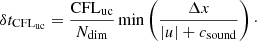
At low Mach numbers, a common drawback of conventional explicit time stepping methods is that for stability the maximum possible time step size δtCFLuc is limited to the acoustic Courant–Friedrich–Lewy (CFL) criterion
 (1)
(1)
Here, Ndim is the number of dimensions, Δx is the grid spacing in the different coordinate directions, u is the fluid velocity and csound is the speed of sound. CFLuc is a dimensionless number which needs to be smaller than unity. The factor 1/Ndim in combination with the minimum over all cells for the cell crossing time in all directions gives a lower limit for the time step. For low-Mach flows, u ≪ csound and the time step size is dominated by the speed of sound. As a consequence, many small time steps are needed to resolve the fluid flow. Although the computational costs for one explicit time step are low, the large number of necessary steps makes explicit time stepping inefficient in this regime.
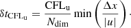
The great advantage of implicit time stepping is that there is no restriction for the step size required for stability. The main constraint arises from the question of how well the flow is to be resolved in time. This leads to the “advective” CFLu criterion which results from Eq. (1) by omitting the speed of sound:
 (2)
(2)
For illustration purposes, setting CFLu = 0.5 corresponds to a time step which does not allow the fluid to cross more than half of a cell per step.
Implicit time integration, however, requires to solve nonlinear systems of equations in each step. This greatly increases the computational costs for one implicit time step compared to explicit time stepping.
In SLH, the family of Explicit first stage, Singly Diagonally Implicit Runge-Kutta (ESDIRK) time steppers is implemented following the description of Hosea & Shampine (1996) and Kennedy & Carpenter (2001). For the simulations in this paper, the ESDIRK23 scheme is applied. It consists of three computing stages and is up to second order accurate in time. This results in two nonlinear systems of equations. SLH applies the Newton-Raphson method which finds their solution in an iterative way. Each iteration itself needs the solution of a linear system of equations. For these, SLH offers a variety of different methods (e.g., Krylov-Subspace schemes and multigrid solvers).
At low Mach numbers, the increased computational costs per time step are overcompensated by the benefit of a larger step size. Numerical tests with SLH imply that implicit time stepping becomes more efficient than explicit time stepping at Mach numbers smaller than about 0.1 to 0.01.
Apart from accuracy requirements, the length of implicit time steps is also limited by the Newton-Raphson solver, which may converge slowly or even diverge if the time step becomes too long. This limit depends on the problem solved and on details of the numerical scheme and needs to be determined experimentally.
The choice of the time step size for the 2D simulation presented in Sect. 4 is discussed in Sect. 4.7 along with an efficiency comparison between implicit and explicit time stepping.
3. Testing internal gravity waves in SLH
In this section, we scrutinize the capability of SLH to correctly reproduce the propagation of IGWs. The base setup is a 2D Cartesian domain containing an isothermal ideal gas in a hydrostatic stratification. A wave packet of small amplitude is evolved for several oscillation periods. The group velocity and the change of the wave shape are then extracted from the simulation and compared to the theoretical prediction which follows from the linear Boussinesq approximation. With this simple but well-defined test setup we verify whether SLH is able to reproduce the prediction accurately enough before applying it to the more complex case of a realistic stellar profile in Sect. 4.
3.1. Boussinesq IGW setup
The theoretical basics of the benchmark test are presented in Appendix A and follow Sutherland (2010). The actual experimental SLH setup closely follows the idea of Miczek (2013) and is extended up to Mach numbers of Ma = 10−2. The basic parameters of the setup are listed in Table 1.
Parameters of the Boussinesq IGW simulation.
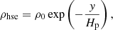
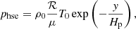
Assuming the ideal gas law p = ρℛ/μT, where ℛ is the universal gas constant, the profiles for density, pressure, and potential temperature in hydrostatic equilibrium are given by
 (3)
(3)
 (4)
(4)
 (5)
(5)
where the pressure scale height Hp is defined as
 (6)
(6)
The Brunt–Väisälä frequency (BVF) according to Eq. (A.10) is spatially constant and reads
 (7)
(7)
We perturb this hydrostatic stratification with a monochromatic internal gravity wave packet. The wavelength λ = 2π/|k|=βHp of the packet is set in terms of the fraction β of the pressure scale height and is inclined by −60° with respect to the horizontal direction. We therefore have
 (8)
(8)
and
 (9)
(9)
We set the vertical domain of the Cartesian box such that it corresponds to 13 times the wavelength λ
 (10)
(10)
in order to provide enough space for the wave to move upward in y-direction. The horizontal extent is set to contain one horizontal wavelength λx = 2π/|kx|, which, in combination with periodic boundary conditions, allows for the plane wave approach. At the top and bottom boundary we apply a layer of two cells which are filled with the hydrostatic initial condition but kept constant in time (constant ghost cells). The amplitude for the vertical velocity component Av is modulated by a Gaussian function according to
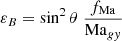
![Mathematical equation: $$ \begin{aligned} A_v({\boldsymbol{x}},t=0) = f_{\mathrm{Ma} }\, \underbrace{\sqrt{\gamma \, \mathcal{R} T_0/\mu }}_{=c_{\mathrm{sound}}}\,\exp { \left[-\frac{1}{2}\left(\frac{y}{\beta H_{\rm p}/2}\right)^{2}\right]}\cdot \end{aligned} $$](/articles/aa/full_html/2020/09/aa37531-20/aa37531-20-eq12.gif) (11)
(11)
The parameter fMa therefore sets the peak Mach number in the vertical velocity amplitude. Using the relations Eqs. (A.11)–(A.13) from the theory described in Appendix A one finds for the initial conditions
 (12)
(12)
 (13)
(13)
 (14)
(14)
 (15)
(15)
where ℜ{.} denotes the real part of a complex expression.
In Appendix A, the time evolution of an initial amplitude modulation of the form of Eq. (11) is derived while considering the IGW dispersion relation Eq. (A.9) up to second order in k. The result given by Eq. (A.28) shows that the initial profile broadens in time and moves at a vertical velocity of
 (16)
(16)
which corresponds to a vertical Mach number of
 (17)
(17)
 (18)
(18)
In Sect. 3.2 we compare the predicted to the simulated evolution of the velocity amplitude to assess the accuracy of our numerical schemes. In order to extract the velocity amplitude function from the simulation, Miczek (2013) suggests the following procedure: It is assumed that the horizontal velocity field can be decomposed as
 (19)
(19)
This is fulfilled for the ansatz Eq. (A.6) and the amplitudes as defined above. Accordingly, also the evolved initial data should at least approximately fulfill this decomposition. However, directly comparing this to the prediction is not straight forward. To simplify the interpretation, the square of Eq. (19) is integrated over the full horizontal width
 (20)
(20)
The integral can be calculated numerically using the data from the simulation and therefore provides the possibility to recover the vertical profile  .
.
The normalized amplitude
 (21)
(21)
then measures the change of the evolved data relative to the maximum of the initial data. In Eq. (21), i and j are the indices in horizontal and vertical direction, respectively; Δx refers to the size of the uniform grid spacing. The velocity by which the peak of rj moves upward is interpreted as the group velocity in Eq. (16).
As discussed in Sect. 4.6, one can define a nonlinearity parameter,
 (22)
(22)
where u and kx denote the horizontal velocity and wave number, respectively. If ε ≳ 1 one expects nonlinear effects to become dominant. Inserting the corresponding expressions into Eq. (22) gives
 (23)
(23)
for the Boussinesq IGWs.
3.2. IGW SLH results
In this section we present simulations of the IGW setup described above for different parameter settings. For comparison, we show the results for the low-Mach solver AUSM+-up and the classical Roe solver (Roe 1981).
The possible parameter space is restricted by two conditions:
-
(a)
We require εB ≪ 1 to stay within the linear regime;
-
(b)
The Boussinesq approximation requires β ≪ 1.
As free parameters we choose εB = 10−2 and vary Magy. The values for β and fMa are then calculated accordingly. This way, we are able to assess the capabilities of both schemes for different Mach numbers. The numerical settings for all of the simulations presented in this section are listed in Table 1. In particular we have chosen the time step size of the implicit time stepping such that the period corresponding to the BVF is resolved by 20 time steps.
We perform simulations for vertical group velocities of Magy = 10−4, 10−3, and 10−2. Whereas condition (b) is well fulfilled for Magy = 10−4, with Magy = 10−2, which is closer to the typical velocity we find in the simulation presented in Sect. 4 (see Fig. 4), we have β = 3 × 10⁻¹ and the stratification does not strictly follow the Boussinesq approximation anymore. Press (1981) shows that for the locally Boussinesq but globally anelastic equations the amplitude scales during the propagation with  where ρ0 is the density at the starting point (cf. Eq. (42)). We therefore multiply equation Eq. (A.28) by the correction factor
 (24)
(24)
to account for the amplification due to varying density.
The results for the AUSM+-up and Roe solvers are visualized in Figs. 1–3, respectively. The left columns show snapshots of the horizontal velocity u at the end of the simulation. The right columns compare at three points in time the amplitude and shape of the vertical velocity distribution as extracted from the simulation using Eq. (21) with the approximate prediction given by Eq. (24) and (A.28).
 |
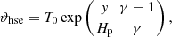
Fig. 1. Results for the IGW test setup as described in Sect. 3 for the AUSM+-up solver (upper row) and the classical Roe solver (lower row). The parameters for the simulation are shown at the top of the plot and described in the main text. Left column: horizontal velocity u in the 2D domain at the end of the simulation at |

In Fig. 1, we have set Magy = 10−4, which corresponds to a vertical velocity amplitude of fMa = 10−6. For the AUSM+-up solver the velocity field in the left column clearly shows the effect of dispersion: waves of longer vertical wavelengths move faster and therefore appear at larger y values compared to smaller vertical wavelengths. The amplitude function broadens over time and is compatible with the prediction in terms of width and peak amplitude. We attribute most of the small deviations from the prediction to our neglect of third order effects in the dispersion relation, which are responsible for the amplitude function’s skew. In contrast, the Roe solver heavily damps the initial amplitude within the first few time steps and it becomes impossible to determine a unique peak in the remaining velocity field. This illustrates that the classical Roe solver fails in the very low Mach regime whereas AUSM+-up still gives excellent results.
We continue by increasing the vertical group velocity to Magy = 10−3. According to Eq. (17) this can only be achieved by increasing β, which sets the fraction of the pressure scale height covered by one wavelength, to β = 3.0 × 10⁻². The results are shown in Fig. 2. The relative peak amplitudes and shapes for AUSM+-up do not change considerably compared to Fig. 1. The results of the Roe solver show distinguishable, but still strongly damped, peaks and their vertical group velocity considerably disagrees with the theoretical prediction.
The effect of increasing the vertical group velocity further to Magy = 10−2 is depicted in Fig. 3: Again, the shape and peak amplitudes for AUSM+-up are compatible with the prediction. For this setup, β = 3 × 10⁻¹ and consequently the density varies noticeably in the simulation volume. This is reflected by the smaller decrease in the expected peak amplitudes in Fig. 3 compared to the amplitudes shown Figs. 1 and 2 for which the amplification according to Eq. (24) is negligible. With the Roe solver, the results are better as compared to those obtained at lower vertical group velocities and the broadening is closer to the prediction. However, significant damping of the velocity amplitude is still evident.
In summary, the results for the classical Roe solver, which we present here solely for comparison, clearly suffer from high damping and show that the wave packages move at the wrong speed. Our tests therefore confirm the need for specialized low-Mach solvers in order to treat IGWs in the regime of velocities below Ma ∼ 10−2. A variety of such solvers are readily available in SLH. A promising example is the AUSM+-up solver for which our tests demonstrate its capability to treat IGW in the low-Mach regime.
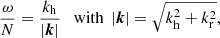
To assess the relevance of this finding we estimate the order of magnitude of the group velocity we expect for the simulation of the real stellar setup presented in Sect. 4. We take the absolute value of Eq. (A.14) and rewrite it in terms of vertical and horizontal components of the wave vector. For the polar coordinates used in the 2D simulation, the horizontal wave number corresponding to the angular degree ℓ is given by
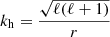 (25)
(25)
and the absolute value of the group velocity is
 (26)
(26)
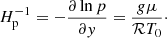
where r denotes the radial position within the model. In Fig. 4 we show the group velocity for ℓ = 4 when inserting the values from the stellar model used in Sect. 4 into Eq. (26). It illustrates that there are large regions at low frequencies with Mach numbers around and below 10−2. These regions become even more extended at higher ℓ-values. We conclude that low-Mach solvers are needed to correctly describe the wave field in simulations such as that presented in Sect. 4, especially in the low-frequency regime dominated by internal gravity waves.
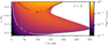 |
Fig. 4. Expected group velocity according to Eq. (26) expressed in terms of Mach number for values of the stellar model used in Sect. 4. Contour lines mark regions of different typical Mach numbers. There are no IGWs for frequencies above the BVF (white area). Instead, one expects the excitation of sound waves only which have Mach numbers of unity. |
4. 2D simulation of a 3 M⊙ ZAMS star
The previous section demonstrates the capabilities of the SLH code and the methods implemented therein to propagate IGWs in the low-Mach regime whereas classical approaches fail. In this section, the SLH code is applied to a real stellar setup, which encompasses both the generation and propagation of IGWs and sound waves.
4.1. Initial model
For the simulation presented here we use the identical initial 1D model as EM19. It describes a nonrotating 3 M⊙ star at the ZAMS with a metallicity of Z = 10−2 and an outer radius of R⋆ = 1.42 × 1011 cm. The model has been calculated with the open-source stellar evolution code MESA (see Paxton et al. 2019 for the latest report on code updates).
The 1D data provided by the MESA model needs to be mapped onto the SLH grid while accurately fulfilling the equation of hydrostatic equilibrium
 (27)
(27)
To do so, we reintegrate Eq. (27) while imposing the radial profile of one thermodynamic quantity from the 1D code (using the 1D density profile for this would be a simple example). All other thermodynamic quantities then follow from the equation of state. The particular choice of the imposed quantity depends on the specific setup. For the case presented here, it is important to keep the position of the convection zone as close as possible to the 1D input MESA model. Convective instability is characterized by a negative sign of the BVF. In regions without any or with only a small gradient in composition (well fulfilled in ZAMS stars) it is essentially determined by the sign of ∇ − ∇ad. Therefore, we follow the approach of Edelmann et al. (2017) to integrate Eq. (27) while enforcing
 (28)
(28)
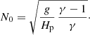
This way the initial spatial extent of the convective zone on the SLH grid exactly matches the 1D input model. Consequently, other quantities might deviate from the 1D model. In Fig. 5 we exemplarily compare the profiles of the SLH model and the 1D input for density and BVF. Both quantities are reproduced reasonably well considering that we cover several orders of magnitudes. There is a deviation of a factor of ten in the convection zone which we attribute to differences in the technical details of the equation of state and the calculations of gradients between MESA and SLH. It is not expected that enforcing  will improve the result as this will only translate the differences into other quantities. However, in the SLH simulation the value of N2 in the convection zone will self-consistently adjust to a value that corresponds to the equilibrium between energy input, for example due to nuclear burning, and the convective flux. The small initial deviation is therefore not relevant. For the BVF, the mean differences in the radiation zone between the 1D MESA model and the mapped profiles is 0.56% with a maximum value of 1.5% at r = 0.87 R⋆ and we therefore consider the applied method to be sufficiently accurate.
 |
Fig. 5. Density (blue) and absolute value of the BVF (orange). The dotted lines correspond to the profiles of the underlying 1D MESA model. The solid lines result from our mapping to the SLH grid. The vertical dashed line marks the radius below which the BVF has a negative sign and one therefore expects convection to develop. The applied mapping method guarantees that the position of the dashed line is identical for the mapped SLH model and the 1D MESA model. |
The underlying 1D MESA model is in thermal equilibrium. The reintegration of Eq. (27) for hydrostatic equilibrium changes the 1D stratification only slightly and we expect the mapped SLH stratification in the radiative envelope to be sufficiently close to the equilibrium model. This, however, is not true for the convective core where we have to artificially boost the nuclear energy release (see Sect. 4.2). A stratification that is not in thermal equilibrium will readjust on the thermal-diffusion time scale τdiff. It can be estimated as (e.g., Maeder 2009)
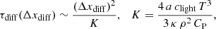 (29)
(29)
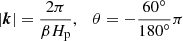
where Δxdiff is a typical length scale. The thermal diffusivity K introduces the radiation constant a = 7.57 × 10⁻¹⁵ erg cm−3 K−4 and the specific heat at constant pressure CP for the ideal gas. The opacity κ is a function of radius and determined by the physical properties of the gas. However, for the mapped SLH model, we set κSLH such that we achieve KMESA = KSLH. Therefore, the value of κSLH is not fully consistent in a physical sense but it allows us to stay closer to the stellar values of thermal diffusion. The blue lines in Fig. 6 show the profiles of κSLH (solid) and κMESA (dashed) and indicate that deviations are reasonably small.
 |
Fig. 6. Blue lines: profiles of the opacity κ for the underlying 1D MESA model (dotted blue line) and the value applied for the mapped 2D SLH model (solid blue line). Orange lines: characteristic diffusion time scale according to Eq. (29) when assuming the radial spacing δr of the SLH grid as typical length scale. |
Following Eq. (29), we estimate the thermal-diffusion time scale taking the radial grid spacing δr to be the typical length scale, see Fig. 6. Due to the energy boosting in the convection zone, deviations from thermal equilibrium are expected to be largest there. From Fig. 6 it can be seen that the diffusion time scale is on the order of 105 h and thus two orders of magnitude larger than what is covered by our 2D simulation (about 103 h, see Sect. 4.2). Furthermore, as the grid spacing δr is already the smallest possible scale, our estimate is a lower limit on the time scale. In the outer parts, the time scale becomes comparable to the simulation time. Thermal flux scales with 1/r in the cylindrical geometry of our 2D simulation (see below for more details on the numerical setup) and therefore differs from the MESA model where spherical geometry is assumed. Thus, the thermal flux is not accurately balanced in our simulation. However, we do not recalculate the equilibrium state while considering the correct scaling of the flux in cylindrical geometry as this would lead to large deviations from the 1D MESA input model. For example, this would likely change the profile of the BVF and therefore alter the dynamics of sound and gravity waves. For our simulations, however, we are interested in waves generated in a stratification as close as possible to a realistic stellar stratification.
From Fig. 6 it is clear that slightly imbalanced initial conditions most probably only impact the very outer part of our model during the course of the 2D simulation. To further validate this, we performed two 1D simulations. Although they do not include convection and wave propagation, they reveal the impact of an imbalanced energy flux. The initial conditions and the numerical settings for both simulations are the same as for the 2D simulation (see text below and Table 2) except that the heat input in the convection zone is turned off. The 1D runs only differ in geometry, which is cylindrical and spherical, respectively, and cover the same time span as the 2D simulation.
Parameters of the 2D simulation.
In the 1D simulations, the maximum change in temperature occurs close to the surface and is only 0.11%. Deviations in the spherical run are slightly smaller but of the same order as in the cylindrical run. Thus, the change is most probably due to the Dirichlet boundary conditions for the temperature which we have chosen for simplicity and that are used for all radial boundaries in the simulations presented here. To exclude any other cause than radiative diffusion for the slight change in the background state we also ran additional 1D simulations where radiative diffusion was disabled. The stratification remains essentially unchanged in these simulations. For the 1D simulations with enabled radiative diffusion, we show the resulting radial profiles of temperature, temperature gradient, and BVF in Fig. B.1 and list the corresponding maximum values in Table B.1.
While the inconsistent treatment of the thermal flux is certainly not desirable, the 1D tests show that its impact on this particular simulation setup is negligible. Nevertheless, for future 2D simulations, we plan to implement the correct geometrical scaling of the flux and to improve the flux boundary conditions.
EM19 do not need to modify the 1D input MESA model. Therefore, Figs. 5 and 6 serve as a direct comparison between the mapped model on the SLH grid and their initial data.
In Table 2 we list the parameters for the SLH simulation. We use 2D polar geometry which corresponds to an infinite cylinder. SLH currently does not support the geometry of a 3D sphere with azimuthal and longitudinal symmetry. Because of the singularity of polar coordinates at r = 0, we cannot include the whole core. The minimum radius of the domain is mainly determined by the decreasing cell sizes in horizontal direction which affects the possible time step size according to the CFL criterion (see Sect. 4.7). We have chosen rmin = 0.007 R⋆ which still allows for reasonably large steps. The upper boundary was set to rmax = 0.91 R⋆ which is close to the value of EM19 who set the upper boundary to 0.9 R⋆. We apply solid-wall boundary conditions at the inner and outer boundaries of the computational domain. They enforce a vanishing velocity perpendicular to the boundary interface. This prohibits mass flux and sound waves from leaving the domain. Periodic boundaries are chosen in the azimuthal direction, which is appropriate since we cover the full azimuthal range of 2π. The number of 960 radial cells ensures that the smallest pressure scale height (close to the outer boundary) is still resolved by 16 grid cells. The number of horizontal grid cells is set such that the cell width at the top of the convection zone δw = δφrtop roughly matches the height δr of the cells, where δφ = 2π/Nφ and δr = (rmax − rmin)/Nr denote the angular and radial resolution, respectively.
4.2. 2D SLH results
For the stellar luminosity as given in the 1D MESA input model, mixing-length theory (MLT, e.g., Kippenhahn et al. 2012) predicts Mach numbers for the convective core of around Ma ∼ 10−4. Simulations in this regime are numerically very challenging and the SLH code has several specialized low-Mach approximate Riemann solvers implemented. However, we have recently noticed that for Mach numbers considerably below 10−3 the convective flow seems not to be driven by heating but rather by numerical instabilities. This problem is subject of ongoing investigations but there is no adequate solution available yet. As a workaround, it was decided to artificially boost the energy generation in order to increase the convective velocity. From MLT one finds that the convective velocity vconv scales with the luminosity L as
 (30)
(30)
which has also been confirmed by numerous numerical studies (e.g., Fig. 7 of Cristini et al. 2019 or Fig. 15 of Andrassy et al. 2019). We boost the stellar luminosity by a factor of 103 which corresponds to a tenfold increase in velocity compared to the MLT prediction. We note that this boosting is still a factor 103 smaller compared to the boosting in the simulations of EM19 and Rogers et al. (2013).
In Fig. 7 we compare the MLT prediction to the results of our 2D simulation. The gray shaded area at small radii marks the region of the core that is convectively unstable according to the Schwarzschild criterion. In the input 1D model, an additional small convection zone near the surface of the star is present but our 2D model already ends at a smaller radius. We find our simulations in good agreement with this “scaled” MLT prediction.
 |
Fig. 7. Predicted and simulated Mach numbers of the 2D model. The orange lines correspond to the MLT prediction: the dashed profile shows the original stellar values, whereas the solid line illustrates the velocities scaled by 10, according to Eq. (30). The blue line shows the 2D results averaged over roughly two convective turnover times, starting at t = 500 h. The profile ends at r ≈ 0.9 R⋆ as our domain does not contain the entire star model. The gray shaded areas mark the convective core and the small region of surface convection in the 1D model. |
However, outside of the convective core a velocity field of considerable amplitude has developed. These velocities are attributed to the excitation and propagation of IGWs and are of main interest for the work presented here. In stark contrast to that, no velocities are assumed in the input 1D model. This illustrates the shortcomings of 1D stellar evolution, where these dynamical phenomena have to be parametrized (see, e.g., Aerts et al. 2019).
The speed of sound in our model ranges from 7 × 107 cm s−1 within the convection zone to 1 × 107 cm s−1 at the top of the computational domain. Accordingly, the Mach number shown in Fig. 7 corresponds to typical velocities of 2 × 105 cm s−1 (convection zone) to 1.3 × 106 cm s−1 (near surface). For the mean convective turnover time in the convection zone  we find
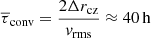 (31)
(31)
where Δrrc = 1.7 × 1010 cm is the depth of the convection zone and vrms the root-mean-square of the absolute velocity. The spatial mean has been taken over the convection zone and the temporal mean includes the entire simulation except for the initial transient phase, where convection has not yet developed (see also Fig. 10). Hence, the 700 h of fully developed convection that we follow in our simulation cover roughly 17 convective turnover times.
The velocity field of the 2D simulation is further illustrated in Fig. 8. It visualizes radial velocity (left panel) and temperature fluctuations from the azimuthal average (right panel). Both quantities are scaled by their horizontal root-mean-square as the amplitudes vary considerably between the outer and inner part of the model. The relative amplitudes have maximum values of four and are approximately equal at all radii for temperature and velocity. In both panels of Fig. 8, the convective core is filled with a few rather coherent structures which correspond to convective eddies that induce wave-like motions. These waves form spiral paths from the point of excitation at the boundary of the convective core as they travel toward the surface. The spatial structures are smaller than those observed by EM19 (see, e.g., their Fig. 8). This is explained by the much smaller effective viscosity of our simulation and further illustrated in Fig. 9 which shows an SLH simulation of a similar domain and resolution but with explicit viscosity and thermal diffusivity comparable to those used by EM19. It is clearly visible how the enhanced diffusive effects even out small scale structures and only large patterns remain.
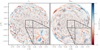 |
Fig. 8. Radial velocity vr and temperature fluctuations Tfluc. As both quantities have larger amplitudes at the outer parts of the model (see further Sect. 4.5) they have been scaled with the corresponding horizontal root-mean-square value at each radius r to ease the visualization. Both panels also show a magnification of the core region. The shown snapshot is taken at t ∼ 580 h. There is also a movie available on https://zenodo.org/record/3819569. |
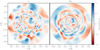 |
Fig. 9. Same quantities as in Fig. 8 but here for a 2D simulation with a viscosity and thermal diffusivity similar to the values used by EM19. We note that the domain for this simulation is comparable to Fig. 8 but not identical. The radial resolution is slightly higher for the viscous simulation and due to the high viscosity the energy input is boosted by 106 in order to get convection starting. |
Figures 7 and 8 illustrate that the fundamental process of generating internal waves, that is a convective core with plumes that excite waves in the radiative envelope, is present in our 2D simulation. In order to further validate our results in the subsequent sections, we closely follow the methods as presented in EM19.
4.3. Frequency spectra
The fundamental properties of stellar oscillations can be probed by investigating their temporal frequency spectrum. For this, we perform a temporal Fourier transformation (FT) of the entire velocity field in our 2D simulation.
The transformation is done for both the radial and horizontal velocity. In order to select waves corresponding to a specific angular degree ℓ, we apply a filter prior to the temporal FT. For the velocity of each stored snapshot, a spatial FT in the angle φ is taken while using all available data points on the grid. Subsequently, all amplitudes are set to zero, except for the one corresponding to the ℓ value we want to filter for. This manipulated spectrum is brought back to real space via an inverse FT. The resulting time sequence of the grid cells of each radial ray is then multiplied by the Hanning window to reduce leakage effects and serves as input for the temporal FT. To reduce the background noise such that individual modes appear more clearly, the temporal spectra are taken for 100 evenly distributed radial rays. The squares of the amplitudes of the resulting Fourier coefficients are then averaged. In principle, the average could be done for all available angles but we experienced no improvement for a larger number of rays. Keeping the numbers of rays low is desirable regarding memory requirements.
The coefficients of the temporal FT are normalized in the same way as in EM19 (see their Eqs. (12) and (13)), essentially the amplitudes are divided by the number of the input data points. This results in coefficients that are independent of the number of bins and that have the same units as the input quantity. Furthermore, for this normalization, the amplitude of a peak across one single frequency bin corresponds to the actual amplitude of that wave in the time domain which eases the direct interpretation of the spectrum. For our spectra, the frequency bins have a width of δf = 1/(700 h) = 0.4 μHz. Spectral lines in our spectra typically (except for a few broad p-modes) span two to four frequency bins and the absolute amplitude is therefore slightly underestimated when directly read off the spectral plots. Finally, the amplitudes are multiplied by a factor of 2 to account for the change in amplitudes in the frequency spectrum due to the application of the Hanning window (see, e.g., Sect. 9.3.9 of Brandt 2011).
We only use the time interval spanning 700 h from 400 h to 1100 h for the spectral analysis (see the gray shaded area in Fig. 10) to avoid the initial development of convection in the core and of the wave field in the envelope.
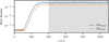 |
Fig. 10. Maximum (blue) and root-mean-square (orange) Mach number in the convection zone as a function of time. The gray shaded area marks the time frame that has been used to extract the spectra that are presented in this paper. |
In Fig. 11 we show the result for the radial velocity, which is the dominant component for p-modes. The upper panel shows the spectrum of the unfiltered velocity, the panels below show the spectra of filtered velocities for some exemplary values of ℓ. This figure is the compressible counterpart of Figs. 24 and 27 in EM19. In Fig. 12, the same quantities are shown for the horizontal velocity which is the dominant component for g-modes. In these plots and in the further course of the paper, a hat denotes quantities that have been obtained using a temporal FT.
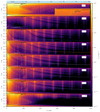 |
Fig. 11. Frequency spectrum of the radial velocity for a time span of 700 h. The normalization is done in a way that the amplitude of a narrow line of one frequency bin width corresponds to the velocity amplitude of the corresponding wave in the time domain. The data is stored in intervals of 480 s. This allows us to capture frequencies up to fmax = 103 μHz with a resolution of δf = 0.4 μHz. In order to reduce the background noise, we show the average of the spectrum of 100 individual radial rays. The doublets for the modes with f ≳ 700 μHz are due to aliasing, which we verified with a simulation with a very short cadence of outputs. The three colored dots in the uppermost panel mark the radii for which the line profiles are shown in Fig. 16. The white and black lines correspond to the BVF at start and end of the simulation, respectively. Colored dashed lines correspond to the Lamb frequencies of different ℓ values according to Eq. (32). In the first row, the uppermost part of the model is magnified (gray box) in order to illustrate the change in the BVF at the end of the simulation. For the magnification, the color scale was adapted to increase the visibility of the lines. We show the spectra for the horizontal velocity in Fig. 12. |
The white line in Fig. 11 indicates the profile of the BVF at the start of the simulation, the black dashed line corresponds to the profile averaged over the last 100 h of the simulation. A magnified vision of the top of the domain is given for ℓ = 0 in the gray box. An oscillatory behavior of the BVF is apparent at the upper boundary of the computational domain which is not removed by the time average. Over time, the oscillations tend to affect a slightly wider range of radii but do not increase their amplitudes considerably. In the 1D simulation (see Sect. 4.1, Fig. B.1, and Table B.1), we find that the change in the BVF is much smaller and does not develop an oscillatory behavior. Thus, the oscillations apparent in the outer parts of the 2D simulation must be due to dynamics that are only captured in multi-dimensional simulations.
While this behavior could be related for example to numerical effects of our boundary conditions, grid resolution, or the transport of angular momentum by propagating IGWs, the exact cause is not fully understood at this point and still subject of ongoing work. However, the deviation is only within a small part of the whole model and we do not expect it to have a significant impact on the general results nor the frequency spectrum of the waves in the envelope below R = 0.8 R⋆. To resolve also the details of the outermost parts more accurately, a more elaborate outer boundary condition is needed as well as a higher resolution to resolve the small scale heights accurately enough.
IGWs can only exist for frequencies below the BVF (see, e.g., Sect. 3.4.2 in Aerts et al. 2010). This property is reflected in the first panel of Fig. 11 by the fact that the whole possible IGW regime (as defined by f < N/2π) shows a significant amplitude which then suddenly drops for f > N/2π. This is in qualitative agreement with Fig. 27 of EM19 and a clear indicator of the excitation of IGWs in the 2D SLH simulation. An increasing number of radial nodes (or, equivalently, a decrease in the radial wavelength) for lower frequencies is another general property of IGWs that is confirmed by the spectra in Fig. 11.
These features have already been seen and described in EM19. However, our simulation also shows additional signals. For ℓ = 0 (second panel in Fig. 11) no IGWs are excited because they cannot be purely radial. Yet, distinct standing modes reaching maximum velocity near the stellar surface are visible at frequencies larger than the BVF. Therefore, they must be signals of excited p-modes.
The colored dashed lines in the panels of Fig. 11 for ℓ > 0 correspond to the respective Lamb frequencies
 (32)
(32)
(e.g., Sect. 3.3.2 of Aerts et al. 2010). They are derived for spherical geometry using spherical harmonics and might not strictly hold in our 2D geometry. However, we still use them here as an estimate to characterize the general behavior of internal waves. A p-mode of angular degree ℓ and frequency fp can only exist if the frequency fulfills the conditions
 (33)
(33)
The corresponding conditions for g-modes are
 (34)
(34)
(see Sect. 3.4 of Aerts et al. 2010 for further details). In regions where the frequency does not fulfill these relations, p- and g-modes are evanescent. This is most easily seen for p-modes in the spectrum for ℓ = 5 and for g-modes in the spectrum for ℓ = 20 in Fig. 11.
The occurrence of p-modes is one of the key differences between fully compressible codes and the anelastic approaches. In the latter, p-modes cannot occur because sound waves are not included in the equations. To bring the p-modes of our 2D simulation into context with observations, we compare them to those of the β Cep stars presented in Aerts & De Cat (2003). They find frequencies at low ℓ typically around f ≈ 6 d−1 ≈ 70 μHz. For the particular star ω1 Sco observations indicate f = 15 d−1 ≈ 174 μHz at ℓ = 9. Of course, the eigenfrequencies of a real star depend on its stellar parameters and excitation mechanism, and β Cep stars have masses typically in the range of 8 M⊙ to 20 M⊙. Thus, the BVFs which set the minimum p-mode frequencies (see Eq. (33)) are smaller compared to our 3 M⊙ model. We find amplitudes associated with p-modes starting at around 300 μHz. Although our model is not directly comparable to the observed β Cep stars, this indicates that the waves, which are excited in our simulations by the convective core, are compatible with those observed in real stars of similar mass. We note, however, that this cannot be seen as a proof for the correctness of the model or the underlying excitation mechanism, especially since p-modes are not typically observed in main-sequence 3 M⊙ stars (Aerts et al. 2010).
For radii deep inside the convection zone (r ≲ 0.14 R⋆) distinct modes are less pronounced in Figs. 11 and 12 (g-modes generally cannot exist there and in our case the Lamb frequencies prohibit also p-modes) but instead amplitudes in a wide range of frequencies appear, a consequence of the turbulent convection in the core. This is most easily seen for larger ℓ values in the spectrum of the horizontal velocity. On the other hand, also at the largest radii, a band of high amplitudes is visible in the uppermost panel which extends over all frequencies. This is due to the development of a shear flow toward the end of the simulation. As it is located very close to the outer boundary, we cannot determine beyond doubt whether the shear flow is caused by the boundary or by deposition of the IGW’s angular momentum due to nonlinear effects. This needs to be examined in more detail in future simulations.
 |
Fig. 12. Frequency spectrum for the horizontal velocity, see Fig. 11 for details. The p-modes are less prominent as their dominant velocity component is radial. |
Another way of illustrating the emerging spectra of waves is given in Fig. 13 (this is similar to Fig. 22 in Herwig et al. 2006 or Fig. 2 in Alvan et al. 2015). Here, the spectrum at a fixed radius r = 0.3 R⋆ is shown for the first 100 ℓ-values. The horizontal blue line indicates the BVF. One clearly observes distinct modes for small ℓ and decreasing mode spacing for increasing ℓ. The amplitudes drop at the BVF as expected for gravity waves. Alvan et al. (2015) estimate a cutoff frequency ωc below which waves have lost a considerable amount of the kinetic energy due to radiative diffusion (see their Eq. (26)). The corresponding profile is shown as dashed white line. They argue that a traveling wave without sufficient energy cannot reach the turning point, travel back and interfere with another progressive wave to form a standing mode. Their corresponding cutoff is rather steep and reaches high frequencies, indicating a wide region where they expect progressive waves. This is similar to Fig. 5 of Rogers et al. (2013). In contrast, for the simulation presented here the profile of ωc is much flatter and stays at much smaller frequencies. It is clear that the excitation of gravity waves from core convection produces an entire spectrum of waves spanning a broad range in frequency.
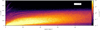 |
Fig. 13. Color map of amplitudes at different frequencies as a function of the angular degree ℓ at a fixed radius of R = 0.3 R⋆. The blue dashed line corresponds to the BVF at this radius. The white dashed line indicates the cutoff frequency ωc below which waves are expected to lose too much kinetic energy due to damping to form standing modes. |
In Fig. 14 we plot the kinetic energies
 (35)
(35)
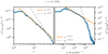 |
Fig. 14. Kinetic energy as a function of angular degree ℓ (left panel) and angular frequency ω (right panel) at the top of the convection zone. Dashed lines correspond to power-law fits. This figure is similar to the second and third column in Fig. 6 of Rogers et al. (2013). |
at the top of the convection zone. Here,  is the velocity at angular degree ℓ and frequency ω which results from the spatial and temporal FT. The sum over all degrees ℓ is terminated at ℓ = 100. The spectra are fitted by power-laws, as proposed in Rogers et al. (2013). Their 2D simulation of a nonrotating model gives similar values for v2(ℓ), shown in our left panel. Also the position of the transition between the two regimes is comparable. However, our profiles for v2(ω) (right panel) are much steeper (Rogers et al. 2013 find ω−1.2 and ω−4.8). In the 2D simulation presented here the transition between the two regimes is at much higher frequencies.
4.4. Dispersion relations
So far we have presented clear indications of the excitation of IGWs and pressure waves. To further confirm this, we show in the following section that the corresponding dispersion relations are fulfilled for both g- and p-modes.
4.4.1. Dispersion for gravity waves
From theory, one finds a dispersion relation for IGWs of the form (e.g., Sect. 3.1.4 Aerts et al. 2010 or Sect. 3.3.3 Sutherland 2010)
 (36)
(36)
where ω = 2πf is the angular frequency of the gravity wave and kh, kr are the horizontal and radial wave numbers. We note that this expression is derived under the assumption of a spatially constant value for the BVF. From Fig. 5 it is clear that this is not the case for the stellar model presented here. Therefore, Eq. (36) is expected to hold only for wavelengths that are short compared to the scale height of the BVF.
To estimate how close our simulation follows Eq. (36), we apply the method of EM19 which is briefly summarized in the following:
The angular frequency ω and BVFare readily available quantities. Because of the spatial FT filtering for specific ℓ, we know that  . The only quantity to determine in Eq. (36) is therefore the vertical wave number kr = 2π/λr or equivalently the radial wavelength λr. To determine the wavelength, the positions of peaks in the amplitude for the FT of the radial velocity are identified for all available frequencies. The distance between adjacent peaks is interpreted as one half of the wavelength at the radial position at the midpoint between the two peaks. We determine the wavelengths starting just above the convection zone until the upper boundary of the model for all frequencies and interpolate in radius afterward. This gives for each frequency f the wavelength λr, f(r). From that, we obtain kr and are finally able to evaluate Eq. (36) in the entire radius-frequency plane for a specific order ℓ.
To visualize the results, the ratio of the left and right side of Eq. (36) is plotted in Fig. 15 exemplarily for ℓ = 2, 4, 10, and 20. Regions in which the dispersion relation is fulfilled, that is the ratio is unity, appear white. This reproduces Fig. 28 of EM19. A magenta line denotes the frequency below which one wavelength is resolved by less than 10 grid points: For a given radial grid spacing δr, the corresponding wave number is kr, n = 10 = 2π/(10 δr) such that this frequency is defined as
 (37)
(37)
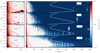 |
Fig. 15. Ratio of the left and right side of the dispersion relation Eq. (36). The method to extract kh/k from the simulation is described in the text. A ratio of unity corresponds to a perfect match and is reflected by white regions. A red color indicates a too large value of kh/k and correspondingly the ratio is too small in blue regions. The white line is the BVF. For frequencies below the yellow line, IGWs are expected to be damped by thermal diffusion. Below the magenta line, the radial wavelength is resolved by less than 10 grid cells. The left column zooms into the low frequency region of the corresponding full plane on the right. The frequency given in the white boxes denotes the value of fmax which sets the scale of the corresponding x-axis. |
The yellow line in Fig. 15 marks the frequency below which one assumes the waves to be dissipated by thermal diffusion. The estimate is based on the equality of the diffusion length and the wavelength at the critical frequency as given by equation1 (27) of EM19. In comparison to EM19, the effect of dissipation is greatly reduced in the SLH simulation. In our case, we are mainly limited by the radial resolution when going to higher ℓ-values. We see agreement with the dispersion relation of linear internal gravity waves everywhere where such agreement can be expected: for modes that are well resolved in space but with radial wavelengths short enough that N2 as well as the radius can be considered approximately constant over a single wavelength. This is the case for low-frequency IGW and gets worse for increasing radial wavelengths, corresponding to increasing frequencies. In contrast to EM19, our results are mainly affected by resolution effects rather than damping, yet broad spectra of standing modes are clearly excited in both numerical setups. For a better visibility, the low frequency regions are magnified in the left column of Fig. 15. At frequencies below 5 μHz, it is difficult to determine if the dispersion relation is fulfilled because the quality of the FT deteriorates as the number of wave periods that fit into the time window of our analysis decreases. However, we are able to reach much smaller frequencies than the anelastic simulations and provide reliable results for wave frequencies above 5 μHz.
Another way of testing the dispersion relation is to measure the inclination of the IGW crests with respect to the radial direction. As the fluid velocity in an internal wave is parallel to the wave crest, we can obtain the inclination by measuring the ratio vh/vr in our simulation. Because the wave vector k is perpendicular to the crests we have
 (38)
(38)
It follows that
 (39)
(39)
and with the aid of Eq. (36) we find the expression
 (40)
(40)
in which the left-hand side can be obtained from the simulation and compared to the theoretical prediction on the right-hand side.
In the top two panels of Fig. 16 we show a line plot representation for the spectra of vr and vh at three different radial positions. They are marked by colored dots in the upper panel of Fig. 11. For radii well above the convection zone, the amplitudes rapidly decrease for f > N/2π. This is expected for a signal mostly made up of IGWs which cannot propagate in this frequency range. Above frequencies of N/2π we can see clearly isolated peaks corresponding to p-modes of various angular degrees. The p-mode amplitudes are at least one order of magnitude smaller than the IGW signal across a broad range of frequencies. For the radial velocity, the spectrum is almost flat with a subtle decrease toward higher frequencies. The spectrum for the horizontal velocity shows a decrease already within the IGW regime. Similar to the findings of EM19, these integrated spectra composed of all angular degrees do not show distinct peaks. However, our results do not have the steep drop in amplitude at very low frequencies as seen in their Fig. 23, which can be attributed to the lower viscosity and thermal diffusivity in our simulation.
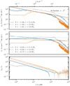 |
Fig. 16. Line plot representations of the spectra for horizontal and vertical velocity at three different radii 0.14 R⋆, 0.4 R⋆, and 0.8 R⋆ are shown in the upper two panels. The dashed lines correspond to the power-law fit as denoted in the labels. The lowest panel shows the ratio of the velocity components at each radius (transparent line) and compares them to the prediction according to Eq. (40) (solid lines). |
In the lowest panel of Fig. 16 we show the ratio of the velocity components as depicted in the two panels above (semitransparent lines). The solid lines represent the prediction given by Eq. (40). There is an excellent agreement for all three radial positions for frequencies below the BVF. The line for 0.14 R⋆ is just beyond the boundary of the convective core and therefore does not follow the steep drop in the ratio as convective motions impact the data. Only for the smallest frequencies the simulation deviates as a result of damping effects and a lack of independent data points for the temporal FT. This result is another strong indication that IGWs are correctly represented in the 2D simulation.
Furthermore, we find the results of our simulations to be comparable to observations of late-B SPB stars. De Cat & Aerts (2002) report the ratio vh/vr for several SPB stars which are typical g-mode pulsators (this corresponds to the K-value in their Fig. 17). The value ranges from 10 to 100. This observed range is similar to the values shown in the lower panel of Fig. 16 for frequencies to the left of the dip, that is below the BVF. For p-mode pulsators De Cat (2002) (see also Aerts & De Cat 2003) reports K-values for β Cep stars which are typically in the range of 0.01−1. Similar values are found in our 2D simulation at frequencies of standing p-modes which is most easily seen as sharp dips at frequencies above the BVF. Such a simplified comparison of values in the interior of our model to the observations at actual stellar surfaces does not allow for a quantitative comparison or stronger conclusions. However, it shows that the wave spectra that self-consistently arise in our hydrodynamical simulation are compatible with observations of oscillations in real stars of similar mass and evolutionary stage (i.e., SPB stars; De Cat & Aerts 2002).
Besides surface velocities, the variation of the disk-averaged luminosity of stars is another observable. It is supposed that contributions from small-scale fluctuations (high ℓ) are suppressed in this quantity as they cancel out on average whereas large-scale contributions are pronounced (e.g., Aerts et al. 2010, Sect. 6). As a simple estimate of this effect we compute the average temperature over half of the circumference of our 2D model prior to the temporal FT. The result is shown as an orange line in Fig. 17 (for comparison, we show as a blue line the spectra which have been averaged similar to the velocity spectra, i.e., only after the temporal FT). At high frequencies, pressure modes appear clearly as individual peaks. This is, however, not the case in the low frequency regime. We note that our spectrum is like those presented in Bowman et al. (2019a, e.g., see their Fig. 3 for the observables of the O star HD 46150 and the figures in their appendix for additional OB stars). The actual situation for observations is more complex than the diagnostic value of our simulations can be. For example, we do not account for limb darkening while this phenomenon comes into play to determine the net flux variation. The limb darkening has more effect for flux observations but far less for the net velocity variations in the line-of-sight. However, our simple experiment illustrates that the net flux variations do not easily reveal any distinct peaks corresponding to low-ℓ modes in the low-frequency regime despite the expected cancellation of the numerous high-ℓ modes.
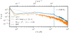 |
Fig. 17. Spectra for temperature at r = 0.80 R⋆. The orange line shows the spectrum of the temperature fluctuations which have been averaged over half of the circumference of our 2D model. The blue line corresponds to the spectra averaged over 100 radial rays after the FT as it is done for the velocity spectra. The dashed blue vertical line denotes the position of the BVF. The gray line corresponds to a power-law fit for the frequencies ranging from 10 μHz to 200 μHz resulting in an exponent of b ≈ −2. |
4.4.2. Dispersion for pressure waves
For the pressure waves, we perform a similar analysis as described in the previous section except that we now check for the usual dispersion relation of pressure waves
 (41)
(41)
The result is shown in Fig. 18 and the colors have the same meaning as in Fig. 15. As expected, the dispersion relation is not fulfilled for f < N/2π. At frequencies corresponding to a standing mode we get a good agreement with predictions from theory. Furthermore, Fig. 18 indicates that pressure modes are excited in the mixed-mode frequency regime, that is between about 200 μHz and 300 μHz. This suggests that a coupling of p- and g-modes is possible. The deviation between standing modes is probably due to the same reasons as discussed in Sect. 4.4.1. This is further illustrated in Fig. B.2 where we show the amplitudes at two specific frequencies. When the frequency matches a standing mode the wavelength can be detected easily whereas this is not possible for frequencies in-between. These results together with the fact that the modes for a particular angular degree are equidistant in frequency in the regime of high-order p-modes give us confidence that the observed modes are indeed p-modes.
 |
Fig. 18. Same quantities as in Fig. 15 but this time for the dispersion relation of sound waves (Eq. (41)). |
4.5. Wave-amplification
From linear theory, one expects the amplification of IGW toward the surface due to density stratification. As shown in Ratnasingam et al. (2019) for spherical geometry, the prediction for IGW amplification is given by (in the notation2 of EM19)
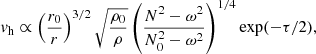 (42)
(42)
where r0 is the starting point of the wave and ρ0, N0 the corresponding density and BVF. The damping factor τ is given by
 (43)
(43)
According to Eq. (42), waves are damped by the effects of thermal dissipation and geometry, but amplified by decreasing density. This ignores the damping effect of viscosity. For consistency, Eq. (42) needs to be multiplied by a correction factor (r0/r)−1/2 to account for our 2D polar geometry of an infinite cylinder, which slightly increases the amplification (Ratnasingam et al. 2020). For the radial velocity, Eq. (42) needs to be scaled according to Eq. (40).
In Fig. 19 we compare the result of Eq. (42) for the 3 M⊙ MESA model to the 2D simulation, similar to Fig. 26 of EM19. For both radial and horizontal velocity, the prediction from linear theory and the simulation are in good agreement for short radial wavelengths and low frequencies (fℓ = 1 = 6.8 μHz, fℓ = 4 = 13.8 μHz), and we assume that the MESA extrapolations toward the surface provide a reasonable estimate of surface velocities. At the highest frequency and longest wavelength (fℓ = 1 = 76.2 μHz) prediction and simulation clearly differ. However, this is expected as the prediction assumes that wavelengths are short compared to all relevant scale heights in the stratification which is clearly not the case for the highest frequency shown in Fig. 19.
 |
Fig. 19. Velocity amplitude for different frequencies and angular degrees ℓ as function of radius. The amplitudes also include the contribution of the two adjacent frequency bins to account for the fact that peaks typically show a width of two to four bins in our simulation. The expected amplification toward the surface according to Eq. (42) is represented by dashed lines; the 1D MESA profile data serve as input variables whereas the starting points are taken as the simulated amplitudes at the first noticeable local maximum of the respective frequency and angular degree. |
Our extrapolation toward larger radii is a very simplified approach and we do not account for the complex physics at the surface, such as the existence of a subsurface convection zone. Therefore, these numbers should only be seen as an approximation to the order of magnitude of the velocity at the surface due to amplified stellar oscillations. The drop in the simulation data at the very top of the computational domain is an artifact of the numerical solid-wall boundary condition whereas the drop in the prediction is an effect of stronger radiative damping near the surface.
Also for the extrapolated velocities at the stellar surface, the order of magnitude for the ratio of the horizontal velocity over the radial one shown in Fig. 19 is compatible with what is found in time-series spectroscopy of g-mode pulsators (De Cat & Aerts 2002).
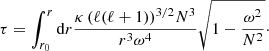
4.6. Nonlinearity parameter
If all waves were to remain in the linear regime, a treatment as in Sect. 4.5 would be a sufficient description of the physics involved. Yet it is expected that the amplification toward the surface causes nonlinearities to become relevant at least in certain ranges of frequency and wavenumber. These nonlinearities lead to a redistribution of energy between different wavenumbers and frequencies. Additionally, wave breaking can cause transport of angular momentum from the core, where the waves are excited, to the envelope.
In Ratnasingam et al. (2019) the effect of different input spectra on the expected nonlinearity of IGWs is examined. The nonlinearity can be estimated by
 (44)
(44)
(Press 1981; Barker & Ogilvie 2010). If ε ≳ 1, nonlinear effects are dominant. However, as demonstrated in Ratnasingam et al. (2020), already rather small values of ε (≈10−3) can cause noticeable energy transfer between different frequencies and wavenumbers.
In Fig. 20 we show the result of Eq. (44) for the amplitudes of the horizontal velocity extracted from the simulation and the extrapolation to the surface as illustrated in Fig. 19. The apparent increase in ε with decreasing frequency is caused by the stronger convective wave excitation at lower frequencies. At even lower frequencies, which are not shown here, wave damping becomes dominant and ε decreases further. For the extrapolated amplitudes we find a maximum value for the nonlinearity parameter of ε = 2.2 for fℓ = 4 = 13.8 μHz.
 |
Fig. 20. Nonlinearity parameter ε according to Eq. (44) for the same frequencies and angular degrees as in Fig. 19. |
From this we conclude that nonlinear effects can be expected at the surface in the frequency regime around 10 μHz. This is further illustrated in Fig. 21, which shows the value for ε at r = 0.4 R⋆ as a function of frequency f and angular degree ℓ. A narrow range around 10 μHz is apparent where the nonlinearity is highest. We note that this looks very similar to Spectrum K and Spectrum LD in Fig. 5 of Ratnasingam et al. (2019) for convective velocity boosted by a factor of three with respect to the stellar models. The strongest nonlinearity in Fig. 21 is seen in the frequency range in which gravity modes have been detected in a sample of about 30 SPB stars in the Kepler data. For all these pulsators, nonlinear behavior has been deduced from the Kepler light curves and a low-frequency IGW power excess has been detected after the removal of the coherent g-modes (Pedersen 2020).
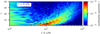 |
Fig. 21. Nonlinearity parameter at r = 0.4 R⋆ for all available frequencies up to an angular degree of ℓ = 40. |
We emphasize that the predictive power for the wave amplification and nonlinearity from this SLH simulation is limited. The boosted energy generation in the core and the accompanying increased velocities also impact the amplitudes of the excited waves. Furthermore, convection is known to be faster in 2D simulations and we apply a simple extrapolation from the upper boundary of our 2D model toward the surface. Nevertheless, we believe that the results presented here at least give an idea of what to expect at the stellar surface where we find indication for the existence of nonlinear effects.
4.7. Time stepping and efficiency
After the detailed evaluation of the properties of the excited waves in the previous sections, the paper is concluded with a discussion of the time step sizes and the efficiency of the SLH code.
In Fig. 22, the radial profiles of the time step size δtCFLuc = 0.5(r) for explicit time stepping (see Eq. (1)) and the maximum implicit time step size δtCFLu = 0.5(r) (see Eq. (2)) are shown for values in the middle of the time span of the 2D simulation. The time step sizes decrease toward the core due to the shrinking azimuthal width of the cells in polar geometry. From the radial profiles, the actual global time step is then given by the minimum over the whole domain. We find min[δtCFLuc = 0.5(r)] = 0.03 s and min[δtCFLu = 0.5(r)] = 21.4 s. Hence, for implicit time stepping, the possible time step size is roughly 700 times larger than the corresponding explicit time step. This might be counter intuitive as the Mach numbers at the surface are of order unity and one would therefore expect implicit time steps to be closer to the explicit step sizes. In that sense, implicit time stepping helps to overcome the general problem of very small step sizes in polar and spherical geometries for large ratios of the outer to the inner radius of the computational domain.
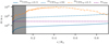 |
Fig. 22. Time step size as a function of radius for different time step criteria. Because of the polar geometry of the grid, the innermost cells become narrower and thus require shorter time steps. The purple dashed horizontal line denotes the time step size of δt = 8 s that is used in the 2D simulation. The dashed vertical line marks the radius below which this step size is larger than a time step size according to Eq. (1) with a CFL number of 50. The gray shaded area indicates the convective region. |
In Miczek (2013), the propagation of a simple 1D sound wave in SLH is compared to predictions from linear wave theory. The simulations are repeated while successively increasing the implicit time step size. In this test setup, sound waves are resolved without noticeable modification if δt ≤ δtCFLuc = 5, whereas they get considerably damped but still propagate at a speed close to the theoretical prediction for δt ≈ δtCFLuc = 50. For δt ≥ δtCFLuc = 500 sound waves cannot be followed at all anymore.
For the 2D simulation presented here, these findings indicate that choosing a time step size of δtCFLu = 0.5 which corresponds to δt ≈ δtCFLuc = 350 at the lower boundary might lead to a strong damping of the sound waves. Although the appropriate time step size clearly depends on the details of the setup and the wavelengths of the considered waves, we follow Miczek (2013) in choosing the time step size in this initial study. As will be shown at the end of this section, this might give a value for the time step size that is too conservative.
For the particular simulation presented here, the time step size is chosen to be δtsim = 8 s (dashed purple horizontal line in Fig. 22). For radii smaller than the vertical line, sound waves are expected to suffer from damping as for these cells the time step is larger than δtCFLuc = 50. This, however, is only a tiny fraction of the whole domain and we do not expect it to have a significant impact on the results. Our choice is a compromise between efficiency and accuracy as will be demonstrated in the following.
To quantify the gain in efficiency when using implicit time stepping, we compare the wall clock time needed to cover a time span of 80 min (2 convective turnover times) when using either implicit or explicit time stepping. For this test, both simulations are restarted at 500 h and all output routines of SLH are disabled in order to minimize possible external effects like a slow file system. We find that the explicit run requires a wall clock time of 37.72 min to perform 15 900 steps on 360 Intel Skylake cores. The implicit run finishes after 6.3 min while performing 600 time steps using the same number of cores. Accordingly, the implicit run is roughly a factor of six faster than the explicit run even though velocities at the top of the computational domain are clearly not in the low-Mach regime, in which implicit time stepping is usually advantageous.
We further compare the efficiency of the SLH code (implicit and explicit) to the pseudo-spectral anelastic SPIN code (EM19). For the comparison, the test runs presented in this section are used for the SLH timings. For the same physical problem, a short test simulation on 300 Ivy Bridge cores for a grid of 1500(r) × 128(ϑ) × 256(φ) serves as input for the SPIN results.
In Table 3, the timings for the two codes to perform one time step per cell and core are listed. From this measure, the explicit SLH mode is roughly a factor of five slower than the SPIN code, potentially reflecting the fact that SLH has not undergone any substantial optimization effort. The implicit SLH mode is 220 times slower than SPIN with a time step size that is only eight times larger. These numbers illustrates that, while our compressible simulations capture the full set of physics described by the full Euler equations, they come with considerably higher computational costs. Because the SPIN and SLH simulations differ in resolution, computational domain, and the energy boosting, a quantitative comparison considering the wall-clock time needed to evolve a cell by one unit of stellar time is not possible here.
Timings for the SLH code (implicit and explicit) and the pseudo-spectral anelastic code SPIN to perform one time step per cell and core.
We note that the settings of the SLH implicit mode may not be optimal yet. As stated by Miczek (2013), fine tuning the linear solver for the specific physical problem to be solved and applying a multigrid solver may lead to improved performance. This is subject of ongoing work and the necessary algorithms are readily available in SLH.
To put the computational costs of the SLH runs into context of 3D simulations, we have performed first preliminary low-resolution 3D simulations of the same initial stratification as used for the 2D simulation in this paper on the JUWELS supercomputer in Jülich, Germany. The domain is discretized in 280(r) × 90(ϑ) × 180(φ) cells while performing time steps of δt = 8 s with the ESDIRK23 implicit time stepping scheme. Based on these runs, we estimate that 8 × 10⁵ core-h will be needed to cover 700 h of simulation time. By scaling this number with the number of grid cells, a simulation with 480 × 180 × 360 cells, which corresponds to half of the resolution of the 2D simulation presented here, needs 5.5 × 10⁶ core-h. The reference simulation applies the same time step size as the finer resolved 2D simulation; therefore, a possible change in the step size is not included in the scaling. However, depending on the desired accuracy, a much larger time step can be chosen and the computational costs decrease correspondingly.
This demand of computational resources is a realistic scenario for applications at HPC facilities. A 3D simulation at the same resolution as the 2D simulation requires 44 × 106 core-h which is at the upper limit of common computing time proposals. However, these numbers show that SLH is efficient enough to perform simulations of stellar oscillations also in 3D for sufficiently long time spans.
As demonstrated, the implicit time stepping improves the efficiency of the SLH code. At the same time it is important to confirm that the accuracy at which sound waves are evolved is sufficient. To this end, we restart the simulation from the 2D implicit run at 500 h and evolve it using an explicit, three-stage Runge-Kutta (RK3) scheme (Shu & Osher 1988) which is third-order accurate in time. The time step is set to δtCFLuc = 0.5, our standard choice for explicit time stepping. The simulation is evolved for 100 h of physical time which corresponds to roughly 80 sound crossing times tcross. We define the sound crossing time to be the time a sound wave needs to travel from the innermost point of the computational domain to the upper boundary,
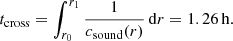 (45)
(45)
We expect the time span of 80 tcross to be sufficient to reveal possible deviations in the spectra.
In Fig. 23, the spectra of the implicit and explicit run are compared at different frequencies corresponding to g- and p-modes. All spectra are based on the same time frame.
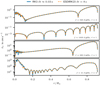 |
Fig. 23. Amplitudes for the radial velocity spectra at four different frequencies for explicit (blue) and implicit (dashed orange) time stepping. The first two frequencies correspond to p-modes whereas the lower two frequencies match g-modes. For radii above the convection zone, the amplitudes completely overlap each other. |
Almost no differences between the amplitudes from implicit and explicit time stepping are visible. This result confirms that the propagation of sound waves is treated correctly also in the implicit run. Furthermore, our implicit time step size of 8 s appears to be a rather conservative choice and larger steps sizes might be possible. This could reduce the computational costs considerably and will be investigated in more detail in future simulations.
5. Conclusion
The main goal of this paper has been to verify the capabilities of the time-implicit, compressible SLH code to correctly treat internal gravity waves (IGWs) and p-modes in stars with a convective core. To this end, two test cases have been considered.
The first test is a simple 2D setup where an IGW packet according to the Boussinesq approximation is evolved in time.
We first simulated the propagation of an IGW packet in a weakly-stratified 2D atmosphere. The initial IGW was set up with different expected group velocities. Velocity distributions were extracted from simulations performed using the low-Mach AUSM+-up solver and the classical Roe solver at a few points in time. The ability of the two solvers to follow IGWs was assessed by comparing the numerical solutions with approximate analytic solutions. The Roe solver revealed strong damping and different broadening of the initial wave packet and the packet’s group velocity was incorrect. These effects were most pronounced at Mach numbers Magy = 10−3. The AUSM+-up scheme showed no significant damping and propagated the packet at a speed close to the prediction. This indicates that a specialized solver is necessary when treating IGWs at low Mach numbers.
Our second test case involving low-Mach-number flows was core hydrogen burning in a 3 M⊙ ZAMS star. We used the same initial 1D model as Edelmann et al. (2019, EM19) to make the simulations comparable. A 2D simulation of this setup was performed using the AUSM+-up solver. The properties of IGW and p-modes were studied following similar methods as in EM19. It was shown that the spectra extracted from the 2D SLH simulations reflect the basic properties of internal waves. A broad spectrum of IGWs is observed for the integrated spectrum whereas individual standing modes can be identified in spectra for single angular degrees ℓ. Modes below the Brunt–Väisälä frequency (BVF) have an increasing radial order with decreasing frequency, a fundamental property of IGWs. Also the dispersion relation extracted from the simulation and the ratios of vertical to horizontal velocities match the theoretical prediction. Furthermore, we find the velocity ratios to be compatible with observational diagnostics from time-series space photometry and high-resolution spectroscopy of slowly pulsating B stars (De Cat & Aerts 2002).
For standing modes above the BVF, the radial order increases with increasing frequency and the dispersion relation matches the one of p-modes. This kind of waves cannot be seen in the anelastic approximation as sound waves are removed from the underlying equations.
Recently, Lecoanet et al. (2019) argued that if the observed variability of stellar surfaces was due to the excitation of IGW from core convection, one would expect to observe distinct peaks in the spectrum which correspond to low ℓ values (see their Fig. 2). We do not see such features in our simulation (see, e.g., Fig. 17). Our explanation for the broad and near-flat profile of IGWs is the same as in EM19: we considered the entire ensemble of waves with large range in radial order and ℓ-values, resulting in small spacings between the resonant frequencies. This “hides” frequency peaks due to individual low-ℓ modes. We clearly see the individual resonant mode frequencies showing up in the simulations when we limit to particular ℓ-values, as illustrated in Figs. 11 and 12. Moreover, stellar rotation, which is not included in the simulations presented here, would cause spectral line splitting and a further increase in the number of lines in the spectrum.
The amplification of the waves toward the surface agrees with the expectation given in Ratnasingam et al. (2019). In SLH, the treatment of IGWs at very low frequencies is mainly limited by radial resolution. In contrast, anelastic simulations are limited by radiative damping and viscous effects already at larger frequencies. Irrespective of the numerical setup, this work and that of EM19 demonstrate the importance of the excitation and propagation of IGWs as a diagnostic tool for the interior physics of stars burning hydrogen in a convective core.
The simulation of the 3 M⊙ model presented here is intended as a proof of concept and aids in the comparison of the simulations of Rogers et al. (2013) and Edelmann et al. (2019). The chosen 2D geometry reduces computational costs and allows for parameter exploration. A validation of 2D results based on selected 3D models is planned for future work. From the cost of preliminary low-resolution 3D simulations we estimated a need of 44 × 106 core-h to simulate a grid with a size of 960(r) × 360(ϑ) × 720(φ) for 700 h physical time. Using only half of the number of cells in each dimension reduces the estimated cost to 5.5 × 10⁶ core-h. These estimates are based on a reference run with the same time step size as the higher resolved 2D simulation presented here. Thus, a change in the time step size is not considered in the scaling. Our tests indicate that the implicit time step size could be increased while still resolving sound waves accurately enough. This could considerably reduce the computational costs. Finally, SLH has already proven an excellent scaling up to a large number of cores (e.g., Edelmann & Röpke 2016) such that this kind of 3D simulations are feasible on modern HPC facilities.
After having tested the methods on the 3 M⊙ model, we will extend our study to higher stellar masses and later evolutionary stages for which there are more observational data. Furthermore, we aim to use the velocity and temporal information from our hydrodynamics data to extract synthetic observables by averaging appropriately over the different wavenumber components. Studying the dependence of wave amplitudes on different luminosity boosting will help us to estimate the amplitudes by extrapolating toward stellar values.
Their equation is missing a factor  . It does not change the result qualitatively but is included here for consistency.
We note that there is an error in the corresponding Eq. (23) of EM19. The expression holds for the horizontal velocity component vh instead of the vertical velocity vr as stated.
Acknowledgments
LH, FKR, and RA acknowledge support by the Klaus Tschira Foundation. PVFE was supported by STFC grant ST/L005549/1 and by the US Department of Energy through the Los Alamos National Laboratory. Los Alamos National Laboratory is operated by Triad National Security, LLC, for the National Nuclear Security Administration of US Department of Energy (Contract No. 89233218CNA000001). This work has been assigned a document release number LA-UR-20-24176. The research leading to these results has received funding from the European Research Council (ERC) under the European Union’s Horizon 2020 research and innovation programme (grant agreement No. 670519: MAMSIE). The authors gratefully acknowledge the Gauss Centre for Supercomputing e.V. (www.gauss-centre.eu) for funding this project by providing computing time through the John von Neumann Institute for Computing (NIC) on the GCS Supercomputer JUWELS at Jülich Supercomputing Centre (JSC). LH thanks Johann Higl for insightful comments. We thank Daniel Lecoanet for useful remarks on the paper and the constructive discussion. We also thank the anonymous referee for very helpful and constructive comments that significantly improved this paper.
References
- Aerts, C., & De Cat, P. 2003, Space Sci. Rev., 105, 453 [CrossRef] [Google Scholar]
- Aerts, C., Christensen-Dalsgaard, J., & Kurtz, D. W. 2010, Asteroseismology (Berlin: Springer) [Google Scholar]
- Aerts, C., Mathis, S., & Rogers, T. M. 2019, ARA&A, 57, 35 [NASA ADS] [CrossRef] [MathSciNet] [Google Scholar]
- Alvan, L., Brun, A. S., & Mathis, S. 2014, A&A, 565, A42 [NASA ADS] [CrossRef] [EDP Sciences] [Google Scholar]
- Alvan, L., Strugarek, A., Brun, A. S., Mathis, S., & Garcia, R. A. 2015, A&A, 581, A112 [NASA ADS] [CrossRef] [EDP Sciences] [Google Scholar]
- Andrassy, R., Herwig, F., Woodward, P., & Ritter, C. 2019, MNRAS, 2556 [Google Scholar]
- Barker, A. J., & Ogilvie, G. I. 2010, MNRAS, 404, 1849 [NASA ADS] [Google Scholar]
- Barsukow, W., Edelmann, P. V. F., Klingenberg, C., Miczek, F., & Röpke, F. K. 2017, J. Sci. Comput., 72, 623 [CrossRef] [Google Scholar]
- Beck, P. G., Bedding, T. R., Mosser, B., et al. 2011, Science, 332, 205 [NASA ADS] [CrossRef] [PubMed] [Google Scholar]
- Beck, P. G., Montalban, J., Kallinger, T., et al. 2012, Nature, 481, 55 [NASA ADS] [CrossRef] [Google Scholar]
- Bedding, T. R., Mosser, B., Huber, D., et al. 2011, Nature, 471, 608 [NASA ADS] [CrossRef] [PubMed] [Google Scholar]
- Bowman, D. M., Aerts, C., Johnston, C., et al. 2019a, A&A, 621, A135 [NASA ADS] [CrossRef] [EDP Sciences] [Google Scholar]
- Bowman, D. M., Burssens, S., Pedersen, M. G., et al. 2019b, Nat. Astron., 3, 760 [NASA ADS] [CrossRef] [Google Scholar]
- Bowman, D. M., Burssens, S., Símon Díaz, S., et al. 2020, A&A, 640, A36 [CrossRef] [EDP Sciences] [Google Scholar]
- Brandt, A. 2011, Noise and Vibration Analysis: Signal Analysis and Experimental Procedures, EBL-Schweitzer (Hoboken, NJ, USA: Wiley) [Google Scholar]
- Briquet, M., Aerts, C., Baglin, A., et al. 2011, A&A, 527, A112 [NASA ADS] [CrossRef] [EDP Sciences] [Google Scholar]
- Burssens, S., Bowman, D. M., Aerts, C., et al. 2019, MNRAS, 489, 1304 [NASA ADS] [CrossRef] [Google Scholar]
- Buysschaert, B., Aerts, C., Bloemen, S., et al. 2015, MNRAS, 453, 89 [NASA ADS] [CrossRef] [Google Scholar]
- Calhoun, D. A., Helzel, C., & Leveque, R. J. 2008, SIAM Rev., 50, 723 [CrossRef] [Google Scholar]
- Cargo, P., & Le Roux, A. 1994, Comptes Rendus de l’Académie des Sciences. Série 1, Mathématique, 318, 73 [Google Scholar]
- Chaplin, W. J., & Miglio, A. 2013, ARA&A, 51, 353 [NASA ADS] [CrossRef] [Google Scholar]
- Colella, P., Dorr, M. R., Hittinger, J. A., & Martin, D. F. 2011, J. Comput. Phys., 230, 2952 [NASA ADS] [CrossRef] [EDP Sciences] [Google Scholar]
- Cristini, A., Hirschi, R., Meakin, C., et al. 2019, MNRAS, 484, 4645 [NASA ADS] [CrossRef] [Google Scholar]
- De Cat, P. 2002, in An Observational Overview of Pulsations in β Cep Stars and Slowly Pulsating B Stars (Invited Paper), eds. C. Aerts, T. R. Bedding, & J. Christensen-Dalsgaard, ASP Conf. Ser., 259, 196 [Google Scholar]
- De Cat, P., & Aerts, C. 2002, A&A, 393, 965 [NASA ADS] [CrossRef] [EDP Sciences] [Google Scholar]
- Edelmann, P. V. F. 2014, Dissertation, Technische Universität München, Germany [Google Scholar]
- Edelmann, P. V. F., & Röpke, F. K. 2016, in JUQUEEN Extreme Scaling Workshop 2016, eds. D. Brömmel, W. Frings, & B. J. N. Wylie, JSC Internal Report No. FZJ-JSC-IB-2016-01, 63 [Google Scholar]
- Edelmann, P. V. F., Röpke, F. K., Hirschi, R., Georgy, C., & Jones, S. 2017, A&A, 604, A25 [NASA ADS] [CrossRef] [EDP Sciences] [Google Scholar]
- Edelmann, P. V. F., Ratnasingam, R. P., Pedersen, M. G., et al. 2019, ApJ, 876, 4 [NASA ADS] [CrossRef] [Google Scholar]
- García, R. A., & Ballot, J. 2019, Liv. Rev. Sol. Phys., 16, 4 [Google Scholar]
- Hekker, S., & Christensen-Dalsgaard, J. 2017, A&ARv, 25, 1 [NASA ADS] [CrossRef] [EDP Sciences] [Google Scholar]
- Herwig, F., Freytag, B., Hueckstaedt, R. M., & Timmes, F. X. 2006, ApJ, 642, 1057 [NASA ADS] [CrossRef] [Google Scholar]
- Hosea, M., & Shampine, L. 1996, Appl. Numer. Math., 20, 21 [CrossRef] [Google Scholar]
- Kennedy, C. A., & Carpenter, M. H. 2001, Additive Runge-Kutta Schemes for Convection-Diffusion-Reaction Equations, Tech. Rep., NASA Technical Memorandum [Google Scholar]
- Kifonidis, K., & Müller, E. 2012, A&A, 544, A47 [NASA ADS] [CrossRef] [EDP Sciences] [Google Scholar]
- Kippenhahn, R., Weigert, A., & Weiss, A. 2012, Stellar Structure and Evolution (Berlin, Heidelberg: Springer-Verlag) [Google Scholar]
- Kurtz, D. W., Saio, H., Takata, M., et al. 2014, MNRAS, 444, 102 [NASA ADS] [CrossRef] [Google Scholar]
- Lecoanet, D., Cantiello, M., Quataert, E., et al. 2019, ApJ, 886, L15 [Google Scholar]
- Liou, M.-S. 2006, J. Comput. Phys., 214, 137 [CrossRef] [MathSciNet] [Google Scholar]
- Maeder, A. 2009, in Physics, Formation and Evolution of Rotating Stars (Berlin, Heidelberg: Springer), Astron. Astrophys. Lib. [Google Scholar]
- Meakin, C. A., & Arnett, D. 2006, ApJ, 637, L53 [CrossRef] [Google Scholar]
- Meakin, C. A., & Arnett, D. 2007, ApJ, 667, 448 [NASA ADS] [CrossRef] [Google Scholar]
- Miczek, F. 2013, Dissertation, Technische Universität München, Germany [Google Scholar]
- Miczek, F., Röpke, F. K., & Edelmann, P. V. F. 2015, A&A, 576, A50 [NASA ADS] [CrossRef] [EDP Sciences] [Google Scholar]
- Mosser, B., Goupil, M. J., Belkacem, K., et al. 2012, A&A, 548, A10 [NASA ADS] [CrossRef] [EDP Sciences] [Google Scholar]
- Pápics, P. I., Tkachenko, A., Van Reeth, T., et al. 2017, A&A, 598, A74 [NASA ADS] [CrossRef] [EDP Sciences] [Google Scholar]
- Paxton, B., Smolec, R., Schwab, J., et al. 2019, ApJS, 243, 10 [NASA ADS] [CrossRef] [PubMed] [Google Scholar]
- Pedersen, M. G. 2020, PhD Thesis, KU Leuven, Belgium [Google Scholar]
- Pedersen, M. G., Chowdhury, S., Johnston, C., et al. 2019, ApJ, 872, L9 [NASA ADS] [CrossRef] [EDP Sciences] [Google Scholar]
- Press, W. H. 1981, ApJ, 245, 286 [NASA ADS] [CrossRef] [Google Scholar]
- Ratnasingam, R. P., Edelmann, P. V. F., & Rogers, T. M. 2019, MNRAS, 482, 5500 [NASA ADS] [CrossRef] [Google Scholar]
- Ratnasingam, R. P., Edelmann, P. V. F., & Rogers, T. M. 2020, MNRAS, 497, 4231 [CrossRef] [Google Scholar]
- Roe, P. L. 1981, J. Comput. Phys., 43, 357 [Google Scholar]
- Rogers, T. M., Lin, D. N. C., McElwaine, J. N., & Lau, H. H. B. 2013, ApJ, 772, 21 [NASA ADS] [CrossRef] [Google Scholar]
- Saio, H., Kurtz, D. W., Takata, M., et al. 2015, MNRAS, 447, 3264 [NASA ADS] [CrossRef] [Google Scholar]
- Shu, C.-W., & Osher, S. 1988, J. Comput. Phys., 77, 439 [Google Scholar]
- Sutherland, B. R. 2010, Internal Gravity Waves (Cambridge: Cambridge University Press) [CrossRef] [Google Scholar]
- Timmes, F. X., & Swesty, F. D. 2000, ApJS, 126, 501 [NASA ADS] [CrossRef] [Google Scholar]
- Van Reeth, T., Tkachenko, A., & Aerts, C. 2016, A&A, 593, A120 [NASA ADS] [CrossRef] [EDP Sciences] [Google Scholar]
- Van Reeth, T., Mombarg, J. S. G., Mathis, S., et al. 2018, A&A, 618, A24 [NASA ADS] [EDP Sciences] [Google Scholar]
Appendix A: Linear theory in Boussinesq approximation
In order to get analytical expressions describing the behavior of IGWs, the fully compressible Euler equations need to be linearized. This can be done in the Boussinesq approximation. It is based on the assumption that pressure and density vary only little in the volume considered. Furthermore, one imposes a time-independent hydrostatic background state and only follows the temporal evolution of deviations from the background state. Additionally, a divergence-free velocity field is assumed. This approach removes the physics of sound waves. For a Boussinesq gas it is convenient to introduce potential temperature ϑ as
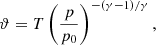 (A.1)
(A.1)
where p0 is the pressure at a specific reference height in the atmosphere with ϑ0, ρ0 (see Sutherland 2010 for a detailed introduction). The two-dimensional equations of motions can then be written as
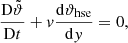 (A.2)
(A.2)
 (A.3)
(A.3)
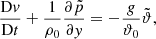 (A.4)
(A.4)
 (A.5)
(A.5)
where quantities with a tilde denote fluctuations from the hydrostatic background state, for instance  . The letters u, v refer to the horizontal and vertical components of the velocity v = (v, u)T. Further, the notation above makes use of the material derivative Dq/Dt = ∂q/∂t + v∇q.
A solution to this set of equations can be found using the ansatz of a 2D plane wave
![Mathematical equation: $$ \begin{aligned} \begin{pmatrix} \tilde{\vartheta }\\ u \\ v \\ \tilde{p} \end{pmatrix} = \begin{pmatrix} A_\vartheta \\ A_u\\ A_v \\ A_p \end{pmatrix} \, \exp {\left[i({\boldsymbol{k}}\cdot {\boldsymbol{x}}) - i\omega t\right]}, \end{aligned} $$](/articles/aa/full_html/2020/09/aa37531-20/aa37531-20-eq62.gif) (A.6)
(A.6)
which introduces the wave vector k = (kx, ky)T, the angular velocity ω, and the complex amplitudes Ai. The absolute values of these amplitudes are assumed to be small, such that terms with products of two or more amplitudes can be neglected. This essentially removes the advection term in the material derivative. Inserting the ansatz into Eqs. (A.2)–(A.5) results in a homogeneous system of linear equations of the form
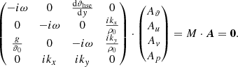 (A.7)
(A.7)
Nontrivial solutions exist only if det(M) = 0 which leads to the dispersion relation for Boussinesq IGWs
 (A.8)
(A.8)
where we have used k ⋅ ex = kx = |k|cos θ with ex being the unit vector in horizontal direction and θ the angle between the wave vector k and the horizontal direction. The dispersion relation is usually written in the form
 (A.9)
(A.9)
where
 (A.10)
is the BVFin the Boussinesq approximation (see, e.g., Sutherland 2010, Sect. 3.2). This result shows that the angular frequency does not depend on the absolute value of the wave vector k and that IGWs do not propagate isotropically. The maximum frequency is ω = N0 for θ = 0° and no purely vertical waves exist as ω = 0 for θ = 90°.
For the specific solution of Eq. (A.7), we set the amplitude of the vertical velocity as free parameter and express the other amplitudes accordingly:
 (A.11)
 (A.12)
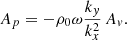 (A.13)
As Eq. (A.7) is a linear system, any superposition of solutions remains a solution to the system. The group velocity of such a wave packet is then given by
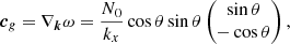 (A.14)
if one uses sin θ = ky/|k|.
In order to describe the time evolution of a wave packet, we follow the methods described in Sutherland (2010, Sect. 1.15) which we generalize to 2D and apply to the specific setup presented in Sect. 3.
In linear theory, a quasi-monochromatic wave packet η(x, t) is usually described as
![Mathematical equation: $$ \begin{aligned} \eta ({\boldsymbol{x}}, t) = \mathcal{A} ({\boldsymbol{x}}, t)\exp \left[ i\left({\boldsymbol{k}}_0\cdot {\boldsymbol{x}} - \omega \left( {\boldsymbol{k}}_0 \right) t\right)\right], \end{aligned} $$](/articles/aa/full_html/2020/09/aa37531-20/aa37531-20-eq71.gif) (A.15)
(A.15)
where the amplitude modulation function 𝒜(x, t) changes much slower in space and time than the exponential function in Eq. (A.15). The wave packet η(x, t) can be represented via a FT as
![Mathematical equation: $$ \begin{aligned} \eta ({\boldsymbol{x}}, t) = \int _{-\infty }^{\infty }\hat{\eta }({\boldsymbol{k}}) \exp \left[i\left({\boldsymbol{k}}\cdot {\boldsymbol{k}} - \omega \left({\boldsymbol{k}}\right)t \right)\right]\,\mathrm{d} {\boldsymbol{k}} \end{aligned} $$](/articles/aa/full_html/2020/09/aa37531-20/aa37531-20-eq72.gif) (A.16)
(A.16)
and, by applying the inverse FT, its spectral representation reads
![Mathematical equation: $$ \begin{aligned} \hat{\eta }({\boldsymbol{k}}) = \frac{1}{(2\pi )^2}\int _{-\infty }^{\infty } \eta ({\boldsymbol{x}}, 0) \exp \left[-i{\boldsymbol{k}}\cdot {\boldsymbol{x}}\right]\, \mathrm{d} {\boldsymbol{x}}. \end{aligned} $$](/articles/aa/full_html/2020/09/aa37531-20/aa37531-20-eq73.gif) (A.17)
(A.17)
From Eqs. (A.15) and (A.17) it further follows that
![Mathematical equation: $$ \begin{aligned} \mathcal{A} ({\boldsymbol{x}}, t)&= \eta ({\boldsymbol{x}},t) \exp \left[-i\left({\boldsymbol{k}}_0\cdot {\boldsymbol{x}} - \omega \left({\boldsymbol{k}}_0\right) t\right)\right] \nonumber \\&=\int _{-\infty }^{\infty }\hat{\eta }({\boldsymbol{k}})\exp \left[i\Delta {\boldsymbol{k}}\cdot {\boldsymbol{x}}\right] \exp \left[-i\Delta \omega t\right] \,\mathrm{d} {\boldsymbol{k}}, \end{aligned} $$](/articles/aa/full_html/2020/09/aa37531-20/aa37531-20-eq74.gif) (A.18)
(A.18)
where Δk = k − k0 and Δω = ω(k) − ω(k0). For t = 0, Eq. (A.18) illustrates that an initial amplitude modulation 𝒜(x, 0) introduces waves with k ≠ k0. Because the wave packet is quasi-monochromatic with a typical wavenumber of k0, the amplitude  must decrease quickly for k ≠ k0. However, in the presence of a nontrivial dispersion relation ω = ω(k), any superposition of waves with different wavenumbers will lead to a broadening of the initial wave packet over time. This will be explicitly shown for the setup presented in Sect. 3.
Here, the initial vertical velocity modulation is a Gaussian as given by Eq. (11):
![Mathematical equation: $$ \begin{aligned} \eta ({\boldsymbol{x}}, 0) = \underbrace{\mathcal{A} _0 \exp \left[-\frac{y^2}{2\sigma ^2}\right]}_{\mathcal{A} ({\boldsymbol{x}}, 0)} \exp \left[i{\boldsymbol{k}}_0\cdot {\boldsymbol{x}}\right] \end{aligned} $$](/articles/aa/full_html/2020/09/aa37531-20/aa37531-20-eq76.gif) (A.19)
(A.19)
with
 (A.20)
Evaluating the FT in Eq. (A.16) leads to
![Mathematical equation: $$ \begin{aligned} \hat{\eta }({\boldsymbol{k}}) = {\delta }(k_x-k_{x,0})\sqrt{2\pi }\sigma \mathcal{A} _0 \exp \left[-\frac{1}{2}\sigma ^2 \Delta k_y^2\right], \end{aligned} $$](/articles/aa/full_html/2020/09/aa37531-20/aa37531-20-eq78.gif) (A.21)
(A.21)
where δ denotes the Dirac delta function. This specific form of η(k) illustrates that a narrower Gaussian modulation in real space leads to a broader distribution in wavenumber space and consequently to a larger dispersion.
From Eqs. (A.18) and (A.21) the time evolution of 𝒜 is determined. To evaluate the FT in Eq. (A.18), we expand the dispersion relation in a Taylor series up to second order
 (A.22)
where we have introduced the abbreviations  for convenience. Inserting Eqs. (A.21) and (A.22) into Eq. (A.18) gives
![Mathematical equation: $$ \begin{aligned} \mathcal{A} ({\boldsymbol{x}}, t) =&\sqrt{2\pi }\sigma \mathcal{A} _0\,\int _{-\infty }^{\infty }\exp \left[i\Delta k_y y\right] \nonumber \\&\times \exp \left[-\frac{1}{2}\sigma ^2\Delta k_y^2 -i\left(\nabla _{{\boldsymbol{k}}}\omega |_{{\boldsymbol{k}}_0}+ \partial ^2_{k_y,k_y}\omega |_{{\boldsymbol{k}}_0}\Delta k_y^2\right)t \right]\,\mathrm{d} k_y. \end{aligned} $$](/articles/aa/full_html/2020/09/aa37531-20/aa37531-20-eq81.gif) (A.23)
(A.23)
This can be simplified to
![Mathematical equation: $$ \begin{aligned} \mathcal{A} ({\boldsymbol{X}}, t) = \sqrt{2\pi }\sigma \mathcal{A} _0 \int _{-\infty }^{\infty } \exp \left[-\frac{\tilde{\sigma }^2}{2}\Delta k_y^2\right]\exp \left[i\Delta k_y Y\right]\,\mathrm{d} k_y, \end{aligned} $$](/articles/aa/full_html/2020/09/aa37531-20/aa37531-20-eq82.gif) (A.24)
(A.24)
by transforming into a moving frame via
 (A.25)
and setting
 (A.26)
The integral in Eq. (A.24) is again the FT of a Gaussian and leads to the final expression
![Mathematical equation: $$ \begin{aligned} \mathcal{A} ({\boldsymbol{X}}, t) = \mathcal{A} _0\,\frac{\sigma }{\tilde{\sigma }}\exp \left[\frac{-Y^2}{2\tilde{\sigma }^2}\right] \end{aligned} $$](/articles/aa/full_html/2020/09/aa37531-20/aa37531-20-eq85.gif) (A.27)
(A.27)
where the absolute value of 𝒜 is given by
![Mathematical equation: $$ \begin{aligned} \left|\mathcal{A} ({\boldsymbol{X}}, t)\right| = \frac{\mathcal{A} _0 \sigma }{\left( \sigma ^4+\left(\partial ^2_{k_y,k_y}\omega |_{{\boldsymbol{k}}_0}t\right)^2 \right)^{1/4}} \cdot \exp \left[-\frac{Y^2}{2} \frac{1}{\sigma ^2 + \left(\frac{\partial ^2_{k_y,k_y}\omega |_{{\boldsymbol{k}}_0}t}{\sigma }\right)^2}\right]\cdot \end{aligned} $$](/articles/aa/full_html/2020/09/aa37531-20/aa37531-20-eq86.gif) (A.28)
(A.28)
Equations (A.27) and (A.28) describe the broadening and decrease in amplitude of an initial Gaussian profile over time when considering the dispersion relation up to second order in k in a system of coordinates moving with the wave packet at its group velocity ∇kω|k0. For the dispersion relation of a Boussinesq IGW according to Eq. (A.9), the group velocity is given by Eq. (A.14) and
 (A.29)
Appendix B: Supplementary plots and tables
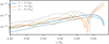 |
Fig. B.1. Relative deviation from the initial profile for the 1D simulations described in Sect. 4.1 at t ∼ 1100 h. Shown are results for the temperature T, the BVF N, and the temperature gradient ∇ = ∂ log T/∂ log P, respectively. Solid lines correspond to cylindrical geometry whereas dashed lines denote the results for spherical geometry. Only the surface of the computational domain is shown to emphasize the change at the outer radial boundary. The deviations are even smaller in the inner part which is not shown here. |
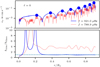 |
Fig. B.2. Check for the dispersion relation of sound waves. Upper panel: amplitudes of the radial velocity at two different frequencies for ℓ = 0. Circles mark radii where our routine detects peaks in the amplitude. The radial wavelengths are then estimated from the distance of neighboring peaks. For the blue line, the frequency matches a standing mode and it shows well defined, distinct peaks. The red line corresponds to a frequency which is between standing modes and shows small-scale incoherent oscillations with many peaks. Lower panel: resulting wave numbers from the simulation are compared to the expectation for sound waves ktheo = 2πf/csound. We find the blue line in good agreement with theory for radii above the convection zone while the red line considerably differs. |
Maximum deviations for the quantities shown in Fig. B.1.
All Tables
Timings for the SLH code (implicit and explicit) and the pseudo-spectral anelastic code SPIN to perform one time step per cell and core.
All Figures
|
Fig. 1. Results for the IGW test setup as described in Sect. 3 for the AUSM+-up solver (upper row) and the classical Roe solver (lower row). The parameters for the simulation are shown at the top of the plot and described in the main text. Left column: horizontal velocity u in the 2D domain at the end of the simulation at |
| In the text | |
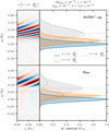 |
Fig. 2. See Fig. 1 for a description of the quantities shown. |
| In the text | |
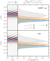 |
Fig. 3. See Fig. 1 for a description of the quantities shown. |
| In the text | |
|
Fig. 4. Expected group velocity according to Eq. (26) expressed in terms of Mach number for values of the stellar model used in Sect. 4. Contour lines mark regions of different typical Mach numbers. There are no IGWs for frequencies above the BVF (white area). Instead, one expects the excitation of sound waves only which have Mach numbers of unity. |
| In the text | |
|
Fig. 5. Density (blue) and absolute value of the BVF (orange). The dotted lines correspond to the profiles of the underlying 1D MESA model. The solid lines result from our mapping to the SLH grid. The vertical dashed line marks the radius below which the BVF has a negative sign and one therefore expects convection to develop. The applied mapping method guarantees that the position of the dashed line is identical for the mapped SLH model and the 1D MESA model. |
| In the text | |
|
Fig. 6. Blue lines: profiles of the opacity κ for the underlying 1D MESA model (dotted blue line) and the value applied for the mapped 2D SLH model (solid blue line). Orange lines: characteristic diffusion time scale according to Eq. (29) when assuming the radial spacing δr of the SLH grid as typical length scale. |
| In the text | |
|
Fig. 7. Predicted and simulated Mach numbers of the 2D model. The orange lines correspond to the MLT prediction: the dashed profile shows the original stellar values, whereas the solid line illustrates the velocities scaled by 10, according to Eq. (30). The blue line shows the 2D results averaged over roughly two convective turnover times, starting at t = 500 h. The profile ends at r ≈ 0.9 R⋆ as our domain does not contain the entire star model. The gray shaded areas mark the convective core and the small region of surface convection in the 1D model. |
| In the text | |
|
Fig. 8. Radial velocity vr and temperature fluctuations Tfluc. As both quantities have larger amplitudes at the outer parts of the model (see further Sect. 4.5) they have been scaled with the corresponding horizontal root-mean-square value at each radius r to ease the visualization. Both panels also show a magnification of the core region. The shown snapshot is taken at t ∼ 580 h. There is also a movie available on https://zenodo.org/record/3819569. |
| In the text | |
|
Fig. 9. Same quantities as in Fig. 8 but here for a 2D simulation with a viscosity and thermal diffusivity similar to the values used by EM19. We note that the domain for this simulation is comparable to Fig. 8 but not identical. The radial resolution is slightly higher for the viscous simulation and due to the high viscosity the energy input is boosted by 106 in order to get convection starting. |
| In the text | |
|
Fig. 10. Maximum (blue) and root-mean-square (orange) Mach number in the convection zone as a function of time. The gray shaded area marks the time frame that has been used to extract the spectra that are presented in this paper. |
| In the text | |
|
Fig. 11. Frequency spectrum of the radial velocity for a time span of 700 h. The normalization is done in a way that the amplitude of a narrow line of one frequency bin width corresponds to the velocity amplitude of the corresponding wave in the time domain. The data is stored in intervals of 480 s. This allows us to capture frequencies up to fmax = 103 μHz with a resolution of δf = 0.4 μHz. In order to reduce the background noise, we show the average of the spectrum of 100 individual radial rays. The doublets for the modes with f ≳ 700 μHz are due to aliasing, which we verified with a simulation with a very short cadence of outputs. The three colored dots in the uppermost panel mark the radii for which the line profiles are shown in Fig. 16. The white and black lines correspond to the BVF at start and end of the simulation, respectively. Colored dashed lines correspond to the Lamb frequencies of different ℓ values according to Eq. (32). In the first row, the uppermost part of the model is magnified (gray box) in order to illustrate the change in the BVF at the end of the simulation. For the magnification, the color scale was adapted to increase the visibility of the lines. We show the spectra for the horizontal velocity in Fig. 12. |
| In the text | |
|
Fig. 12. Frequency spectrum for the horizontal velocity, see Fig. 11 for details. The p-modes are less prominent as their dominant velocity component is radial. |
| In the text | |
|
Fig. 13. Color map of amplitudes at different frequencies as a function of the angular degree ℓ at a fixed radius of R = 0.3 R⋆. The blue dashed line corresponds to the BVF at this radius. The white dashed line indicates the cutoff frequency ωc below which waves are expected to lose too much kinetic energy due to damping to form standing modes. |
| In the text | |
|
Fig. 14. Kinetic energy as a function of angular degree ℓ (left panel) and angular frequency ω (right panel) at the top of the convection zone. Dashed lines correspond to power-law fits. This figure is similar to the second and third column in Fig. 6 of Rogers et al. (2013). |
| In the text | |
|
Fig. 15. Ratio of the left and right side of the dispersion relation Eq. (36). The method to extract kh/k from the simulation is described in the text. A ratio of unity corresponds to a perfect match and is reflected by white regions. A red color indicates a too large value of kh/k and correspondingly the ratio is too small in blue regions. The white line is the BVF. For frequencies below the yellow line, IGWs are expected to be damped by thermal diffusion. Below the magenta line, the radial wavelength is resolved by less than 10 grid cells. The left column zooms into the low frequency region of the corresponding full plane on the right. The frequency given in the white boxes denotes the value of fmax which sets the scale of the corresponding x-axis. |
| In the text | |
|
Fig. 16. Line plot representations of the spectra for horizontal and vertical velocity at three different radii 0.14 R⋆, 0.4 R⋆, and 0.8 R⋆ are shown in the upper two panels. The dashed lines correspond to the power-law fit as denoted in the labels. The lowest panel shows the ratio of the velocity components at each radius (transparent line) and compares them to the prediction according to Eq. (40) (solid lines). |
| In the text | |
|
Fig. 17. Spectra for temperature at r = 0.80 R⋆. The orange line shows the spectrum of the temperature fluctuations which have been averaged over half of the circumference of our 2D model. The blue line corresponds to the spectra averaged over 100 radial rays after the FT as it is done for the velocity spectra. The dashed blue vertical line denotes the position of the BVF. The gray line corresponds to a power-law fit for the frequencies ranging from 10 μHz to 200 μHz resulting in an exponent of b ≈ −2. |
| In the text | |
|
Fig. 18. Same quantities as in Fig. 15 but this time for the dispersion relation of sound waves (Eq. (41)). |
| In the text | |
|
Fig. 19. Velocity amplitude for different frequencies and angular degrees ℓ as function of radius. The amplitudes also include the contribution of the two adjacent frequency bins to account for the fact that peaks typically show a width of two to four bins in our simulation. The expected amplification toward the surface according to Eq. (42) is represented by dashed lines; the 1D MESA profile data serve as input variables whereas the starting points are taken as the simulated amplitudes at the first noticeable local maximum of the respective frequency and angular degree. |
| In the text | |
|
Fig. 20. Nonlinearity parameter ε according to Eq. (44) for the same frequencies and angular degrees as in Fig. 19. |
| In the text | |
|
Fig. 21. Nonlinearity parameter at r = 0.4 R⋆ for all available frequencies up to an angular degree of ℓ = 40. |
| In the text | |
|
Fig. 22. Time step size as a function of radius for different time step criteria. Because of the polar geometry of the grid, the innermost cells become narrower and thus require shorter time steps. The purple dashed horizontal line denotes the time step size of δt = 8 s that is used in the 2D simulation. The dashed vertical line marks the radius below which this step size is larger than a time step size according to Eq. (1) with a CFL number of 50. The gray shaded area indicates the convective region. |
| In the text | |
|
Fig. 23. Amplitudes for the radial velocity spectra at four different frequencies for explicit (blue) and implicit (dashed orange) time stepping. The first two frequencies correspond to p-modes whereas the lower two frequencies match g-modes. For radii above the convection zone, the amplitudes completely overlap each other. |
| In the text | |
|
Fig. B.1. Relative deviation from the initial profile for the 1D simulations described in Sect. 4.1 at t ∼ 1100 h. Shown are results for the temperature T, the BVF N, and the temperature gradient ∇ = ∂ log T/∂ log P, respectively. Solid lines correspond to cylindrical geometry whereas dashed lines denote the results for spherical geometry. Only the surface of the computational domain is shown to emphasize the change at the outer radial boundary. The deviations are even smaller in the inner part which is not shown here. |
| In the text | |
|
Fig. B.2. Check for the dispersion relation of sound waves. Upper panel: amplitudes of the radial velocity at two different frequencies for ℓ = 0. Circles mark radii where our routine detects peaks in the amplitude. The radial wavelengths are then estimated from the distance of neighboring peaks. For the blue line, the frequency matches a standing mode and it shows well defined, distinct peaks. The red line corresponds to a frequency which is between standing modes and shows small-scale incoherent oscillations with many peaks. Lower panel: resulting wave numbers from the simulation are compared to the expectation for sound waves ktheo = 2πf/csound. We find the blue line in good agreement with theory for radii above the convection zone while the red line considerably differs. |
| In the text | |
Current usage metrics show cumulative count of Article Views (full-text article views including HTML views, PDF and ePub downloads, according to the available data) and Abstracts Views on Vision4Press platform.
Data correspond to usage on the plateform after 2015. The current usage metrics is available 48-96 hours after online publication and is updated daily on week days.
Initial download of the metrics may take a while.