| Issue |
A&A
Volume 641, September 2020
Planck 2018 results
|
|
|---|---|---|
| Article Number | A2 | |
| Number of page(s) | 33 | |
| Section | Cosmology (including clusters of galaxies) | |
| DOI | https://doi.org/10.1051/0004-6361/201833293 | |
| Published online | 11 September 2020 | |
Planck 2018 results
II. Low Frequency Instrument data processing
1
AIM, CEA, CNRS, Université Paris-Saclay, 91191 Gif-sur-Yvette, France; AIM, Université Paris Diderot, Sorbonne Paris Cité, 91191 Gif-sur-Yvette, France
2
APC, AstroParticule et Cosmologie, Université Paris Diderot, CNRS/IN2P3, CEA/lrfu, Observatoire de Paris, Sorbonne Paris Cité, 10 rue Alice Domon et Léonie Duquet, 75205 Paris Cedex 13, France
3
African Institute for Mathematical Sciences, 6-8 Melrose Road, Muizenberg, Cape Town, South Africa
4
Astrophysics Group, Cavendish Laboratory, University of Cambridge, J J Thomson Avenue, CB3 0HE Cambridge, UK
5
Astrophysics & Cosmology Research Unit, School of Mathematics, Statistics & Computer Science, University of KwaZulu-Natal, Westville Campus, Private Bag X54001, 4000 Durban, South Africa
6
CITA, University of Toronto, 60 St. George St., M5S 3H8 Toronto, ON, Canada
7
CNRS, IRAP, 9 Av. colonel Roche, BP 44346, 31028 Toulouse Cedex 4, France
8
Cahill Center for Astronomy and Astrophysics, California Institute of Technology, Pasadena, CA 91125, USA
9
California Institute of Technology, Pasadena, CA, USA
10
Computational Cosmology Center, Lawrence Berkeley National Laboratory, Berkeley, CA, USA
11
Département de Physique Théorique, Université de Genève, 24 quai E. Ansermet, 1211 Genève 4, Switzerland
12
Departamento de Astrofísica, Universidad de La Laguna (ULL), 38206 La Laguna, Tenerife, Spain
13
Departamento de Física, Universidad de Oviedo, C/ Federico García Lorca, 18, Oviedo, Spain
14
Departamento de Física Matematica, Instituto de Física, Universidade de São Paulo, Rua do Matão, 1371 São Paulo, Brazil
15
Departamento de Matemáticas, Universidad de Oviedo, C/ Federico García Lorca, 18, Oviedo, Spain
16
Department of Astrophysics/IMAPP, Radboud University, PO Box 9010, 6500 GL Nijmegen, The Netherlands
17
Department of Mathematics, University of Stellenbosch, Stellenbosch 7602, South Africa
18
Department of Physics & Astronomy, University of British Columbia, 6224 Agricultural Road, Vancouver, British Columbia, Canada
19
Department of Physics & Astronomy, University of the Western Cape, 7535 Cape Town, South Africa
20
Department of Physics, Gustaf Hällströmin katu 2a, University of Helsinki, Helsinki, Finland
21
Department of Physics, Princeton University, Princeton, NJ, USA
22
Department of Physics, University of California, Santa Barbara, CA, USA
23
Department of Physics, University of Illinois at Urbana-Champaign, 1110 West Green Street, Urbana, IL, USA
24
Dipartimento di Fisica e Astronomia G. Galilei, Università degli Studi di Padova, via Marzolo 8, 35131 Padova, Italy
25
Dipartimento di Fisica e Scienze della Terra, Università di Ferrara, Via Saragat 1, 44122 Ferrara, Italy
26
Dipartimento di Fisica, Università La Sapienza, P.le A. Moro 2, Roma, Italy
27
Dipartimento di Fisica, Università degli Studi di Milano, Via Celoria, 16, Milano, Italy
28
Dipartimento di Fisica, Università degli Studi di Trieste, via A. Valerio 2, Trieste, Italy
29
Dipartimento di Fisica, Università di Roma Tor Vergata, Via della Ricerca Scientifica, 1, Roma, Italy
30
European Space Agency, ESAC, Planck Science Office, Camino bajo del Castillo, s/n, Urbanización Villafranca del Castillo, Villanueva de la Cañada, Madrid, Spain
31
European Space Agency, ESTEC, Keplerlaan 1, 2201 AZ Noordwijk, The Netherlands
32
Gran Sasso Science Institute, INFN, viale F. Crispi 7, 67100 L’Aquila, Italy
33
Haverford College Astronomy Department, 370 Lancaster Avenue, Haverford, PA, USA
34
Helsinki Institute of Physics, Gustaf Hällströmin katu 2, University of Helsinki, Helsinki, Finland
35
INAF – OAS Bologna, Istituto Nazionale di Astrofisica – Osservatorio di Astrofisica e Scienza dello Spazio di Bologna, Area della Ricerca del CNR, Via Gobetti 101, 40129 Bologna, Italy
36
INAF – Osservatorio Astronomico di Padova, Vicolo dell’Osservatorio 5, Padova, Italy
37
INAF – Osservatorio Astronomico di Trieste, Via G.B. Tiepolo 11, Trieste, Italy
38
INAF, Istituto di Radioastronomia, Via Piero Gobetti 101, 40129 Bologna, Italy
39
INAF/IASF Milano, Via E. Bassini 15, Milano, Italy
40
INFN – CNAF, viale Berti Pichat 6/2, 40127 Bologna, Italy
41
INFN, Sezione di Bologna, viale Berti Pichat 6/2, 40127 Bologna, Italy
42
INFN, Sezione di Ferrara, Via Saragat 1, 44122 Ferrara, Italy
43
INFN, Sezione di Milano, Via Celoria 16, Milano, Italy
44
INFN, Sezione di Roma 1, Università di Roma Sapienza, Piazzale Aldo Moro 2, 00185 Roma, Italy
45
INFN, Sezione di Roma 2, Università di Roma Tor Vergata, Via della Ricerca Scientifica, 1, Roma, Italy
46
Imperial College London, Astrophysics group, Blackett Laboratory, Prince Consort Road, SW7 2AZ London, UK
47
Institut d’Astrophysique Spatiale, CNRS, Univ. Paris-Sud, Université Paris-Saclay, Bât. 121, 91405 Orsay Cedex, France
48
Institut d’Astrophysique de Paris, CNRS (UMR7095), 98bis boulevard Arago, 75014 Paris, France
49
Institute Lorentz, Leiden University, PO Box 9506, 2300 Leiden, RA, The Netherlands
50
Institute of Astronomy, University of Cambridge, Madingley Road, CB3 0HA Cambridge, UK
51
Institute of Theoretical Astrophysics, University of Oslo, Blindern, Oslo, Norway
52
Instituto de Astrofísica de Canarias, C/Vía Láctea s/n, La Laguna, Tenerife, Spain
53
Instituto de Física de Cantabria (CSIC-Universidad de Cantabria), Avda. de los Castros s/n, Santander, Spain
54
Istituto Nazionale di Fisica Nucleare, Sezione di Padova, via Marzolo 8, 35131 Padova, Italy
55
Jet Propulsion Laboratory, California Institute of Technology, 4800 Oak Grove Drive, Pasadena, CA, USA
56
Jodrell Bank Centre for Astrophysics, Alan Turing Building, School of Physics and Astronomy, The University of Manchester, Oxford Road, M13 9PL Manchester, UK
57
Kavli Institute for Cosmological Physics, University of Chicago, Chicago, IL 60637, USA
58
Kavli Institute for Cosmology Cambridge, Madingley Road, CB3 0HA Cambridge, UK
59
LERMA, CNRS, Observatoire de Paris, 61 avenue de l’Observatoire, Paris, France
60
LERMA/LRA, Observatoire de Paris, PSL Research University, CNRS, Ecole Normale Supérieure, 75005 Paris, France
61
Laboratoire de Physique Subatomique et Cosmologie, Université Grenoble-Alpes, CNRS/IN2P3, 53 rue des Martyrs, 38026 Grenoble Cedex, France
62
Laboratoire de Physique Théorique, Université Paris-Sud 11 & CNRS, Bâtiment 210, 91405 Orsay, France
63
Lawrence Berkeley National Laboratory, Berkeley, CA, USA
64
Low Temperature Laboratory, Department of Applied Physics, Aalto University, Aalto, 00076 Espoo, Finland
65
Max-Planck-Institut für Astrophysik, Karl-Schwarzschild-Str. 1, 85741 Garching, Germany
66
Mullard Space Science Laboratory, University College London, RH5 6NT Surrey, UK
67
NAOC-UKZN Computational Astrophysics Centre (NUCAC), University of KwaZulu-Natal, 4000 Durban, South Africa
68
Nicolaus Copernicus Astronomical Center, Polish Academy of Sciences, Bartycka 18, 00-716 Warsaw, Poland
69
SISSA, Astrophysics Sector, via Bonomea 265, 34136 Trieste, Italy
70
San Diego Supercomputer Center, University of California, San Diego, 9500 Gilman Drive, La Jolla, CA 92093, USA
71
School of Chemistry and Physics, University of KwaZulu-Natal, Westville Campus, Private Bag X54001, 4000 Durban, South Africa
72
School of Physical Sciences, National Institute of Science Education and Research, HBNI, 752050 Jatni, Odissa, India
73
School of Physics and Astronomy, Cardiff University, Queens Buildings, The Parade, CF24 3AA Cardiff, UK
74
School of Physics and Astronomy, Sun Yat-sen University, 2 Daxue Rd, Tangjia, Zhuhai, PR China
75
School of Physics and stronomy, University of Nottingham, NG7 2RD Nottingham, UK
76
School of Physics, Indian Institute of Science Education and Research Thiruvananthapuram, Maruthamala PO, Vithura, 695551 Thiruvananthapuram Kerala, India
77
Simon Fraser University, Department of Physics, 8888 University Drive, Burnaby, BC, Canada
78
Sorbonne Université-UPMC, UMR7095, Institut d’Astrophysique de Paris, 98bis boulevard Arago, 75014 Paris, France
79
Space Science Data Center – Agenzia Spaziale Italiana, Via del Politecnico snc, 00133 Roma, Italy
80
Space Sciences Laboratory, University of California, Berkeley, CA, USA
81
The Oskar Klein Centre for Cosmoparticle Physics, Department of Physics, Stockholm University, AlbaNova, 106 91 Stockholm, Sweden
82
UPMC Univ Paris 06, UMR7095, 98bis boulevard Arago, 75014 Paris, France
83
Université de Toulouse, UPS-OMP, IRAP, 31028 Toulouse Cedex 4, France
84
Warsaw University Observatory, Aleje Ujazdowskie 4, 00-478 Warszawa, Poland
Received:
24
April
2018
Accepted:
4
September
2018
Abstract
We present a final description of the data-processing pipeline for the Planck Low Frequency Instrument (LFI), implemented for the 2018 data release. Several improvements have been made with respect to the previous release, especially in the calibration process and in the correction of instrumental features such as the effects of nonlinearity in the response of the analogue-to-digital converters. We provide a brief pedagogical introduction to the complete pipeline, as well as a detailed description of the important changes implemented. Self-consistency of the pipeline is demonstrated using dedicated simulations and null tests. We present the final version of the LFI full sky maps at 30, 44, and 70 GHz, both in temperature and polarization, together with a refined estimate of the solar dipole and a final assessment of the main LFI instrumental parameters.
Key words: space vehicles: instruments / methods: data analysis / cosmic background radiation
Corresponding author: D. Maino, This email address is being protected from spambots. You need JavaScript enabled to view it.
© ESO 2020
1. Introduction
This paper is part of the 2018 data release (PR3) of the Planck1 mission, and reports on the Low Frequency Instrument (LFI) data processing for the legacy data products and cosmological analysis. The 2018 release is based on the same data set as the previous release (PR2) in 2015, in other words, a total of 48 months of observation (eight full-sky Surveys), more than three times the nominal mission length of 15.5 months originally planned (Planck Collaboration I 2011).
This paper describes in detail the complete data flow through the LFI scientific pipeline as it was actually implemented in the LFI data-processing centre (DPC), starting from the basic steps of handling raw telemetry (for both scientific and house-keeping data), and ending with the creation of frequency maps and validation of the released data products (similar information for the High Frequency Instrument [HFI] can be found in Planck Collaboration III 2020). Since this is the last Planck Collaboration paper on the LFI data analysis, in this introduction we provide a pedagogical description of all the data-processing steps in the pipeline. Later sections report in greater detail on those pipeline steps that have been updated, modified, or improved with respect to the previous data release. For the many steps that remain unchanged, the interested reader should consult Planck Collaboration II (2016).
Processing LFI data is divided into three main levels (see Fig. 1). In Level 1, the process starts with the ingestion of the required information from the telemetry data packets and auxiliary data received from the Mission Operation Centre; both the science and housekeeping information is then transformed into a format suitable for Level 2 processing.
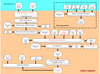 |
Fig. 1. Schematic representation of the LFI data-processing pipeline from raw telemetry down to frequency maps. Elements in red are those changed or improved with respect to Planck Collaboration II (2016). |
The goal of Level 2 is the creation of calibrated maps at all LFI frequencies in both temperature and polarization, with known systematic and instrumental effects removed. Finally, Level 3 requires the combination of both LFI and HFI data to perform astrophysical component separation (both CMB and foregrounds), extraction of CMB angular power spectra, and determination of cosmological parameters. This last level is not described in this paper: we refer readers to (Planck Collaboration I 2020; Planck Collaboration IV 2020; Planck Collaboration V 2020; Planck Collaboration VI 2020).
Level 2 includes three main blocks of the analysis pipeline: TOI processing or “preprocessing”; calibration; and mapmaking. Preprocessing starts with flagging data that were made unusable due to lost telemetry packets and spacecraft manoeuvres. It continues with corrections for nonlinearity in the analogue-to-digital converters (ADCs) and for small spurious electronic signals at 1 Hz. The ADCs convert analogue output voltages from the detectors into digital form. Any departure from exact linearity creates a distortion in the response curve of the radiometer. The current implementation of the algorithm to correct for ADC nonlinearity includes improvements made since Planck Collaboration II (2016), which are described in Sect. 2. The 1 Hz electronic spikes result from an unwanted, low-level interaction between the electronic clock and the science data, and occur in the data-acquisition electronics after the acquisition of raw data from the radiometer diodes, and before ADC conversion (Meinhold et al. 2009; Mennella et al. 2010, 2011). They appear as a 1 Hz square wave, synchronous with the on-board time signal. The procedure for correcting the data is the same as described in Planck Collaboration II (2016), and consists of fitting and subtracting a 1 Hz square wave template from the time-domain data.
In the pseudo-correlation scheme adopted for the LFI radiometers (Bersanelli et al. 2010), each radiometer diode produces an alternating sequence of sky and reference load signals at the 4096 Hz phase-switch frequency. The 1/f noise of the sky and reference data streams are highly correlated. Subtracting the optimally scaled reference data stream from the sky data stream reduces the 1/f noise in the sky data by several orders of magnitude. We calculate this optimal gain modulation factor (GMF) using the same method as for the 2015 release (Planck Collaboration II 2016).
The last preprocessing step is diode combination. This reduces the impact of imperfect isolation between the two diodes of each LFI radiometer. The weighted combinations are unchanged since the 2015 release, and may be found in Table 3 of Planck Collaboration II (2016); typical values range between 0.4 and 0.6 (a perfect diodes isolation would yield 0.5 equal weights).
The pointing pipeline runs in parallel with the preprocessing pipeline just described. It uses the focal plane geometry, the spacecraft velocity and attitude, and “PTCOR” a long-time-scale pointing correction (which takes account of both the distance from the Sun and thermometry from the Radiometer Electronics Box Assembly). The pointing pipeline reconstructs the pointing position and horn orientation for each sample in the data stream. PTCOR is unchanged from the 2015 release, and is described in Planck Collaboration I (2016).
The next step in the pipeline is photometric calibration. In addition to the pointing and sky-minus-load differences, auxiliary information is required to obtain accurate calibration. This includes the 4π beam response, a model of the CMB dipole together with the time-varying modulation of its amplitude induced by the motion of the spacecraft along its orbit – our primary calibration source – and a model of Galactic emission whose contribution through the beam far sidelobes is modelled and subtracted from each time line. The calibration process converts raw voltages at the output of the radiometers into thermodynamic temperatures. The basic calibration reference signal is the Planck dipole convolved with the full 4π beam response, properly weighted according to the bandpass of each radiometer. The Planck dipole used in this step is identical to the one employed in the earlier 2015 release (Planck Collaboration I 2016, see further details in the following sections). On the other hand, the calibration algorithm has been significantly improved compared to the previous release by including Galactic emission along with the CMB dipole in the calibration model. This is particularly important during periods when the spacecraft spin axis is nearly aligned with the CMB dipole, and the variation of the dipole signal along scan circles is small (“dipole minima”). The final gain solution is obtained with an iterative destriper, DaCapo, which at each step determines radiometer gains, constraining the data to fit the dipole + Galaxy beam-convolved model. The output gain solutions are noisy during dipole minima (especially in Surveys 2 and 4). Therefore, as in the previous release (but with further optimization), we employ an adaptive smoothing algorithm that reduces scatter in gain solutions, but preserves real discontinuities caused by abrupt changes in the radiometer operating conditions. Finally, these smoothed gain solutions are applied to raw data streams, after subtraction of both the dipole and an estimated signal contributed by Galactic emission into the beam sidelobes.
The final step of the Level 2 pipeline is mapmaking, in other words, using the calibrated data and pointing information to create Stokes I, Q, and U maps of the sky at each frequency. The LFI mapmaking code is Madam, fully described in Keihänen et al. (2005) and Planck Collaboration VI (2016), which removes correlated 1/f noise with a destriping approach. Correlated noise is modelled as a single baseline (Maino et al. 2002). The algorithm makes use of the redundancy in the observing strategy to constrain these baselines, which are then subtracted from the time-ordered data in the creation of the sky maps. The algorithm allows a selection of baseline lengths, which is always a compromise between optimal noise removal and computational cost. As in the 2015 release, we adopt baselines of 1 s at 44 and 70 GHz, and 0.25 s at 30 GHz. The shorter baseline at 30 GHz is appropriate for the higher 1/f noise of the radiometers at this frequency (see Table 1), which introduces a larger correlated component in the noise.
LFI performance parameters.
Table 1 gives typical values for the main instrument performance parameters measured in flight; similar tabulations were given in previous releases. Beam and optical properties are derived from Jupiter transits, and are consistent with 2015 results. Major improvements in the calibration uncertainty are reflected in more stable results for noise parameters. Values reported are averages among the radiometers operating at a given frequency. At 44 GHz the FWHM is not entirely representative of the actual beamwidth, since one of the three 44 GHz horns is located on the opposite site of the focal plane from the other two (Planck Collaboration IV 2016).
2. Time-ordered information (TOI) processing
The main changes in the Level 1 pipeline since the last release are related to data flagging and to correcting the nonlinearity in the analogue-to-digital converter (ADC).
We revised our flagging procedure to use more conservative and rigorously homogeneous criteria. The new procedure results in a slightly higher flagging rate, particularly during the first 200 operational days (ODs) of the mission; however, the fraction of flagged data remains negligible. Table 2 gives final values for the missing and unusable data for the full mission; changes from the release reported in Planck Collaboration II (2016) are a fraction of one percent. Since the fraction of flagged data is negligible, so the effect on science is also negligible. It is worth mentioning that although the LFI radiometers are quite stable, there are occasional jumps in gain that if not treated properly would impact the calibration procedure well beyond the single data point in which the jump occurs. These jumps are now properly identified and taken into account.
Percentage of LFI observation time lost due to missing or unusable data, and to manoeuvres.
Nonlinearity in the ADCs that convert analogue detector voltages into numbers distorts the radiometer response, possibly mimicking a sky signal. For the present release, we developed a new approach to the correction of this effect that produces significantly better results at 30 GHz.
The first step in the correction is calculation of the white-noise amplitude, given by the difference between the sum of the variances and twice the covariances of adjacent samples in the time-stream. Specifically, ![Mathematical equation: $ \sigma^2_{\mathrm{WN}} = {\mathrm{Var}}[X_{\rm o}] + {\mathrm{Var}}[X_{\rm e}] - 2 {\mathrm{Cov}}[X_{\rm o},X_{\rm e}] $](/articles/aa/full_html/2020/09/aa33293-18/aa33293-18-eq2.gif) , where Xo and Xe are data points with time-stream odd and even indices respectively. ADC nonlinearity produces a variation in the white-noise amplitude as a function of the detector voltage.
, where Xo and Xe are data points with time-stream odd and even indices respectively. ADC nonlinearity produces a variation in the white-noise amplitude as a function of the detector voltage.
In the previous release, we fitted the white-noise amplitudes binned with respect to detector voltage with a simple spline curve, and translated the results into a correction curve as described in Appendix A of Planck Collaboration III (2014). For this release, we tried a more physically motivated fitting function based on the fact that ADCs suffer from a linearity error ε on each bit. We modelled the output voltage V0 as
 (1)
(1)
where bi is 1 if the ith bit is set and 0 otherwise, εi is the linearity error of the ith bit (which is between −0.5 and +0.5), Vadu is the voltage step for one binary level change (one analogue-to-digital unit or adu), and Voff allows for a possible offset (see Figs. 9 and 10 of Planck Collaboration III 2014). Due to complex degeneracies in Eq. (1), we adopted an annealed optimization procedure to avoid local minima in the χ2 fit to this model.
Even this improved model proved to be too simple, however, as it did not reproduce some of the asymmetries present in the original ADC curve, which appeared to be due to coupling between adjacent bits. We therefore add to the previous expression an extra summation for adjacent coupled bits:
 (2)
(2)
where εi, i + 1 is the coupled error between bits i and i + 1.
We compared the results between this method and the previous one by means of null maps, checking the consistency of the resulting new gain solution with the new ADC correction applied. This was done by computing the rms scatter from the eight different survey maps, taking into account pixel hits and zero levels. A “goodness” parameter can then be derived from the mean level of the masked null map made between these survey scatter maps.
The null maps showed substantial improvement at 30 GHz, but little improvement at 44 and 70 GHz. Inspection of the ADC solutions revealed that the higher noise per radiometer and low ADC nonlinearity at 70 GHz did not allow for a good fit. At 44 GHz, on the other hand, the ADC effect was so large that the new model could not reproduce some of the details, and so led to some small residuals. The 30 GHz system has much lower noise and less thermal drift in the gain, meaning that more voltage levels were revisited more often, yielding a more consistent ADC model curve. It was therefore decided to keep the new solution only for the 30 GHz channels. The other two frequencies thus have the same correction for ADC nonlinearity as in the previous release.
3. Photometric calibration
The raw output from an LFI radiometer is a voltage, V, which we can write (Planck Collaboration II 2016) as
![Mathematical equation: $$ \begin{aligned} V(t) = G(t) \times \left[ B *(D_{\mathrm{solar} } + D_{\mathrm{orbital} } + T_{\mathrm{sky} }) + T_0\right], \end{aligned} $$](/articles/aa/full_html/2020/09/aa33293-18/aa33293-18-eq5.gif) (3)
(3)
where G is the gain B encodes both convolution with a 4π instrumental beam and the observation scanning strategy, Dsolar and Dorbital are the solar and orbital CMB dipoles2, Tsky represents the sum of the CMB and foreground fluctuations, and T0 is the sum of the 2.7 K CMB temperature, other astrophysical monopole terms, and any internal instrumental offsets. Photometric calibration is the process of determining G(t) accurately over time, which is critical for the quality of the final maps.
In the Planck 2013 release, based on 15 months of data, an accurate Planck determination of Dorbital was not possible, and G(t) was estimated from Dsolar alone. We used the best-fit, 9 year WMAP dipole estimate as the reference model against which to compare the measured voltages (Planck Collaboration V 2014; Bennett et al. 2013). Successive analyses (Planck Collaboration XXXI 2014; Planck Collaboration I 2016) showed that this model resulted in gain estimates that were offset by about 0.3% (due largely to foreground contamination in the WMAP dipole), within the originally estimated error uncertainty.
In the Planck 2015 release, we implemented internal and self-consistent estimation of the solar dipole by using the orbital dipole for absolute calibration (see Sect. 4 for further details). The orbital dipole is much smaller than the solar dipole, but is known absolutely with exquisite accuracy from the orbital motion of Planck itself. This resulted in relative calibration uncertainties ≲0.3% (Planck Collaboration II 2016), adequate to allow high-precision cosmology based on temperature measurements. However, for polarization even a relative error of 10−3 is non-negligible, and a large fraction of the LFI work on data quality since the 2015 release has revolved around reducing this error further.
As discussed extensively in Planck Collaboration II (2016) and Planck Collaboration XI (2016), one of the most notable problems in the 2015 LFI processing was the failure of a specific internal null test, namely that taken between Surveys 1, 3, 5, 6, 7, and 8, and Surveys 2 and 4. In particular, Surveys 2 and 4 showed significantly larger uncertainties in their gain estimation than the other Surveys (see Fig. 4 in Planck Collaboration II 2016), and, critically, they also showed significant excess B-mode power on the very largest scales. Although it was well-known that Surveys 2 and 4 happen to be aligned with the Planck scanning strategy in such a way that the dipole modulation reaches very low minima, thus exacerbating the impact on calibration of any potential systematic effect, we could not identify the specific source of the anomaly. Nevertheless, because of the null-test failure, those two surveys were removed from the final polarization maps and likelihood analysis.
Since that time, we have performed a series of detailed end-to-end simulations designed specifically to identify the source of this null-test failure, and this work ultimately led to a minor, but important, modification of the calibration scheme outlined above and described in detail in Planck Collaboration II (2016). In short, the survey null-test failure was due to not accounting for the polarized component of the sky signal in Eq. (3). This has now been done, as described in detail below. Thus the updated calibration scheme represents the logical conclusion of Eq. (3), since we now account for all terms as far as we are able to model them.
3.1. Joint gain estimation and component separation
Before describing the updated calibration scheme, we first establish some useful intuition regarding the physical effect in question. We start with the raw gains, G(t), as measured in 2015 (Planck Collaboration II 2016). Overall, this function may be crudely modelled over the course of the mission as a sum of a linear term and a 1-year sinusoidal term:
 (4)
(4)
where the four free parameters, {a,b,c,d}, must be fitted radiometer by radiometer. From this model, we compute the “normalized fractional gain” as
 (5)
(5)
This function is simply the fractional gain excess (or deficit) relative to a smoothly varying model, expressed as a percentage.
Each LFI horn feeds two independent polarization-sensitive radiometers with polarization angles rotated 90° with respect to each other (Planck Collaboration II 2014); these are called “M” (main) and “S” (side), respectively. Since two such radiometers are often susceptible to the same instrumental effects (thermal, sidelobes, etc.), it is useful to study differences between them to understand instrumental systematic effects. For example, Fig. 2 shows the difference in normalized fractional gain for two 30 GHz radiometers, namely  . Other 30- and 44 GHz radiometers show qualitatively similar behaviour, at the sub-percent level, whereas the 70 GHz radiometers behave differently, for reasons explained below. The following discussion therefore applies in detail only to the 30 and 44 GHz radiometers, while the 70 GHz radiometers will be treated separately.
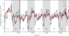 |
Fig. 2. Normalized gain difference (see main text for precise definition) between two radiometers inside the same horn (28M and 28S here) as a function of pointing ID for both the 2015 (DX11D) and 2018 calibration schemes. The coloured lines show this function for the various iterations in the new {gain-estimation + mapmaking + component separation} calibration scheme. Sky surveys are indicated by alternating white and grey vertical bands. Other 30- and 44 GHz radiometers show qualitatively similar behaviour, whereas the 70 GHz radiometers exhibit too much noise, and corresponding iterations for these detectors do not converge within this scheme. |
3.2. Calibration at 30 and 44 GHz
The black curve in Fig. 2 shows the normalized gain difference for the default 2015 orbital dipole-based calibration scheme (DX11D), and exhibits a striking oscillatory pattern with a period equal to one survey. Such a pattern is very difficult to explain instrumentally, since the two radiometers reside inside the same horn, while it is consistent with the effect of polarized foregrounds. Since the polarization angles of the two radiometers are rotated by 90°, any polarized signal on the sky will at any given time be observed with opposite signs by the two radiometers. Strong polarized foregrounds therefore lead to the kind of difference shown in Fig. 2, with a sign given by the relative orientation of the satellite and the Galactic magnetic field. Furthermore, this difference will be repeatable across surveys. This is confirmed by simulations – inserting a polarized foreground sky into end-to-end simulations induces precisely the same pattern as shown here.
The solution to this problem is to include the sky signal, Tsky, in the calibrator, on the same footing as the orbital and solar dipoles, including both temperature and polarization fluctuations. This is non-trivial, since the purpose of the experiment is precisely to measure the polarized emission from the sky. A good approximation can be established, however, through an iterative process that alternates between gain calibration, map making, and astrophysical component separation, using the following steps.
-
0.
Let Tsky be the full best-fit (Commander-based; Eriksen et al. 2008; Planck Collaboration X 2016) Planck 2015 astrophysical sky model, including CMB, synchrotron, free-free, thermal and spinning dust, and CO emission for temperature maps, plus CMB, synchrotron, and thermal dust in polarization.
-
1.
Estimate G from Eq. (3), explicitly including the temperature and polarization component of Tsky in the calibration on the same footing as Dsolar and Dorbital.
-
2.
Compute frequency maps with these new gains.
-
3.
Determine a new astrophysical model from the updated frequency maps using Commander (at present the sky model is adjusted only for LFI frequencies).
-
4.
Iterate steps (1) to (3).
Since the true sky signal is stationary on the sky, while the spurious gain fluctuations are not, this process will converge, essentially corresponding to a generalized mapmaker in which the G(t) is estimated jointly with the sky maps. Alternatively, this process may also be considered as a Gibbs sampler that in turn iterates through all involved conditional distributions, and thereby converges to the joint maximum likelihood point (Eriksen et al. 2008).
The process is, computationally expensive, however; each iteration takes about one week to complete. For practical purposes, the current process was therefore limited to four full iterations (not counting the 2015 model used for initialization). The normalized gain differences established in each iteration are shown as coloured curves in Fig. 2 for the same radiometer pair as discussed above (for example 28M and 28S). Here we see that most of the effect is accounted for simply by introducing a rough model, as already the first iteration is significantly flatter than the initial model (black versus blue curves). Subsequent iterations make relatively small differences, and, critically, the differences between consecutive iterations become smaller by almost a factor of 2 in each case, indicating that the algorithm indeed converges.
While the most obvious oscillatory pattern in the initial model has been eliminated by the introduction of the astrophysical sky model, it is not clear whether a smaller contribution remains. In Fig. 3 we therefore show the same functions, but now with all surveys stacked together. Explicitly, the coloured regions in Fig. 3 represent the mean and standard deviations as evaluated over the eight surveys. Since the surveys have slightly different lengths, the stacking is done such that the starting pointing periods of the surveys are aligned, and longer surveys are truncated at the end. These stacked functions will tend to suppress random signals across surveys, but highlight those common to all eight surveys. As before (but now more clearly), we see that the 2015 model (grey band) exhibits a highly significant Survey-dependent pattern. This pattern is greatly suppressed simply by adding a rough model to the calibrator (blue band). And the pattern is additionally reduced by further iterations, with a convergence rate of about a factor of 2 per iteration.
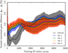 |
Fig. 3. Same as Fig. 2, but stacked over surveys. Each band corresponds to the mean and 1σ confidence region as evaluated from eight surveys. |
To understand the convergence rate in more detail, we show in Fig. 4 the differences in polarization amplitude between two consecutive iterations of the full 30 GHz map. The top panel shows the difference between the second and first iterations; the middle panel shows the difference between the third and second iterations; and, finally, the bottom panel shows the difference between the fourth and third iterations. As anticipated, here we see that the magnitude of the updates decreases by a factor of 1.5–2 at high latitudes.
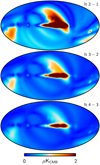 |
Fig. 4. Polarization amplitude difference maps between consecutive iterations of the internal foreground model evaluated at 30 GHz, as derived with Commander. The three panels show the differences between: the second and first iterations (top); the third and second iterations (middle); and the fourth and third iterations (bottom). All maps are smoothed to an effective angular resolution of 8° FWHM. |
In addition to the decreasing amplitude with iterations, it is also important to note that the morphology of the three difference maps is very similar, and dominated by a few scans that align with Ecliptic meridians. In other words, most of the gain uncertainty is dominated by a few strong modes on the sky, and the iterations described above largely try to optimize the amplitude of these few modes. Furthermore, as seen in Figs. 2–4, it is clear that we have not converged to numerical precision with only four iterations. Due to the heavy computational demand of the iterative process, we could not produce further steps. As a consequence, we expect that low-level residuals are still present in the 2018 LFI maps, with a pattern similar to that of the 2015 maps, though with significantly lower amplitude. For the 2018 release, we adopt the difference between the two last iterations as a spatial template of residual gain uncertainties projected onto the sky. This template is used only at 70 GHz.
3.3. Calibration at 70 GHz
As already mentioned, the above discussion applies only to the 30- and 44 GHz radiometers, since the 70 GHz radiometers behave differently. The reason for this may be seen in Fig. 5, which simply shows the final co-added 30-, 44-, and 70 GHz frequency maps, downgraded to HEALPix (Górski et al. 2005) Nside = 16 resolution (3 8 × 3
8 × 3 8 pixels) to enhance the effective signal-to-noise ratio per pixel. The grey regions show the Galactic calibration mask used in the analysis, within which we do not trust the foreground model sufficiently precisely to use it in gain calibration, primarily due to bandpass leakage effects (Planck Collaboration II 2016). Here we see a qualitative difference between the three frequency maps: while both the 30- and 44 GHz polarization maps are signal-dominated, the 70 GHz channel is noise-dominated. This has a detrimental effect on the iterative scheme described above, ultimately resulting in a diverging process; essentially, the algorithm attempts to calibrate on noise rather than actual signal.
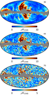 |
Fig. 5. Final low-resolution LFI 2017 polarization amplitude sky maps. From top to bottom, the panels show the co-added 30-, 44-, and 70 GHz frequency maps. The grey regions indicate the mask used during gain calibration. Each pixel is 3 |


For this channel, we therefore retain the same calibration scheme used in 2015, noting that the iterative algorithm fails because the foregrounds are weak at this channel. While this is a problem when using foregrounds directly as a calibrator, it also implies that foregrounds are much less of a problem than in the other channels. In place of an iterative scheme, we adopt the corresponding internal differences described above, obtained at 30 GHz, as a tracer of gain residuals also for the 70 GHz channel (shown in Fig. 6), and marginalize over this spatial template in a standard likelihood fit in pixel space. Indeed, we provide this additive template as part of the LFI 2018 distribution, with a normalization given by a best-fit likelihood accounting for both CMB and astrophysical foregrounds. Thus, the best-fit amplitude of the provided template is unity. For all the cosmological analysis involving the 70 GHz channel and presented in this final Planck data release we accounted for gain residuals by subtracting this correction. Therefore we strongly recommend to do the same for any other cosmological investigation involving the 70 GHz frequency channel.
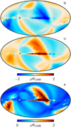 |
Fig. 6. Gain correction template for the 70 GHz channel in terms of Stokes Q (top) and U (middle), and the polarization amplitude, P (bottom). The template is smoothed to 2° FWHM, and its amplitude is normalized to the best-fit value derived in a joint maximum likelihood analysis of both the CMB power spectrum and template fit, as described in the text. |
We started this discussion by recalling the failure reported in Planck Collaboration II (2016) of a null test between Survey sets {1,3, 5–8} and {2, 4}. In Fig. 7 we therefore compare this particular null map as derived with the old (top panel) and new (bottom panel) calibration schemes. The improvement is obvious, with most fluctuations in the latter appearing consistent with noise. The remaining excesses appear on angular scales compatible with the smoothing scale of 8° FHWM, and are consistent with the position of known variable point sources. A direct comparison with WMAP frequency maps suggests similar improvements; see Appendix A for details.
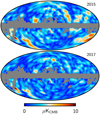 |
Fig. 7. 30 GHz polarization amplitude null maps evaluated between survey combinations {S1,S3, S5–8} and {S2, S4} for both the 2015 (top) and 2018 (bottom) calibration schemes. This particular survey split is maximally sensitive to residual gain uncertainties from polarized Galactic foreground contamination because of the orientation of the scanning strategy employed in Surveys 2 and 4; see text and Planck Collaboration II (2016) for further details. Both maps are smoothed to an effective angular resolution of 8° FWHM. |
4. The LFI dipole
The calibration signal for LFI is the dipole anisotropy due the motion of the solar system relative to the CMB. Precise knowledge of the amplitude and direction of the 3.3 mK solar dipole, however, requires another absolutely defined signal. This is given by the orbital dipole, the time-varying 200 μK modulation of the dipole amplitude induced by the motion of the spacecraft in its yearly orbit around the Sun (including the small velocity component due to the spacecraft orbit around L2). As the amplitude and orientation of the orbital dipole can be determined with exquisite accuracy from the satellite telemetry and orbital ephemeris, it is the best absolute calibration signal in all of microwave space astrophysics. It should be emphasized that the dipole determination is primarily a velocity measurement, and that the actual dipole amplitude is derived from the velocity assuming a value for the absolute temperature of the CMB; together with HFI (Planck Collaboration III 2020) we use the value T0 = 2.72548 K (Fixsen 2009).
4.1. Initial calibration to determine the amplitude and direction of the solar dipole
These two dipoles are merged into a single signal at any given time, but they can be separated over the course of the mission, since the solar dipole is fixed on the sky while the orbital dipole varies in amplitude and direction with the satellite velocity as it orbits the Sun. It is therefore possible to base the calibration entirely on the orbital dipole alone. As in the previous release (Planck Collaboration II 2016), we omit the solar dipole from the fit but retain the far-sidelobe-convolved orbital dipole and the fiducial dipole convolved again with far sidelobes, and also remove the restriction of having no dipole signal in the residual map. In this way, the solar dipole is extracted as a residual, and its amplitude and position can be determined. In this section we discuss the LFI 2018 measurements of the solar dipole and compare them to other measurements.
For accurate calibration, we have to take into account two effects that behave like the orbital dipole, in the sense that they are linked to the satellite and not to the sky: polarized foregrounds; and pick-up in the far sidelobes. While the orbital dipole calibration is robust against unpolarized foregrounds, the polarized part of the foregrounds depends on the orientation of the satellite. Similarly, the far sidelobes are also locked to the direction in which the satellite is pointing.
The corrections for polarized foregrounds are made directly in the timelines by unrolling the Q and U frequency maps from the previous internal data release, in other words, projecting them into timelines according to the scanning strategy and beam orientation, and also taking into account the gain calibration factor derived from an initial calibration run. We find that only one iteration is required to remove the polarized signal, with further iterations in this cleaning process making no difference. The amplitude of the polarized signal removed is about 40 μK at 30 GHz, 15 μK at 44, and 4 μK at 70 GHz, mainly due to the North Polar Spur and the Fan regions.
In the previous dipole analysis, the far sidelobes were removed using the GRASP beam model but reduced to the lowest multipoles to obtain the expected, properly convolved dipole signal for both the orbital and solar dipoles. In the calibration code now used (DaCapo; Planck Collaboration II 2016), we fit for the orbital dipole convolved with far sidelobes, as well as for the convolution of the solar dipole with the far sidelobes. In such a way, we force a pure dipole (without far sidelobes) into the residual map. However, we found that far-sidelobe pick-up was not completely removed, which resulted in a trend in the dipole amplitude with horn position on the focal plane, as well as small differences between the orbital and solar dipole calibration factors. By adjusting the direction of the large-scale compoment of the far sidelobes, we find a correction between 1 and 10 μK, depending on horn focal plane position, which brings both calibration factors together and, simultaneously, removes the asymmetry in the focal plane.
To calibrate on the orbital dipole, we need to mask the strong emission from the Galactic plane. The mask is generated using a 5 deg-smoothed 30 GHz intensity map with different threshold cut-offs, which result in different sky fractions. The orbital calibration is carried out using a sky fraction of 94%, since this calibration is robust to the intensity of unpolarized foregrounds. For the analysis of the resultant dipole maps, we use instead an 80% sky fraction, accounting for the presence of unpolarized foregrounds in the residual maps. An even more conservative mask with a sky fraction of 60% gives about 15% more scatter in the dipole position between channels, but not in any systematic way. This is consistent with a lower signal-to-noise ratio due to the poorer sky coverage. The actual fit is performed with a Markov chain Monte Carlo (MCMC) approach, where we search for dipole position and amplitude as well as the amplitudes of synchrotron, dust, and free-free templates derived from Commander (Planck Collaboration X 2016). We performed several tests, varying the amplitude of the mask (ranging from 60% to 80% sky fraction), with and without point source masks, in the derivation of the foreground templates. We found that use of a mask with 80% sky fraction and masked foregrounds reduces the scatter in the dipole estimation at 70 GHz by about 15%.
4.2. The solar dipole
From the MCMC samples, the 1% and 99% values are used to set the limits on the dipole amplitude and position. Figure 8 shows results for the three LFI frequencies for both dipole direction (upper panel) and amplitude (lower panel). There is a clear trend with frequency in dipole direction, due to foreground contamination. As expected, the 70 GHz channel has the lowest foreground signal, and it is used to derive the final LFI dipole. With respect to the previous release, the use of the small far-sidelobe correction has removed the systematic amplitude variation with focal plane position. Thus the cross-plane null pairs that were used in the previous release are not needed. This results in a smaller scatter of both dipole positions and derived amplitude, as shown in the bottom panel. For each LFI data point we report two error bars: the small (red) one is the actual error in the fit (also reported in Table 3); and the large (black) one is obtained by summing the calibration error in quadrature. The grey band represents the WMAP derived dipole amplitude, for comparison. Numerical results are summarized in Table 3, where single radiometer errors are derived from the MCMC samples. The final uncertainty in the LFI dipole derived from only the 70 GHz
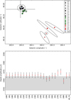 |
Fig. 8. Direction (top) and amplitude (bottom) of the solar dipole determined from each of the LFI detectors. Uncertainties in direction are given by 95% ellipses around symbols, colour-coded for frequency (70 GHz black or unfilled, 44 GHz green, and 30 GHz red). The four discrepant points are at 30 GHz, where we expect foregrounds affect dipole estimation. Amplitude uncertainties are dominated by the systematic effects of gain uncertainties. The grey band in the bottom panel shows the WMAP dipole amplitude for comparison. |
Dipole characterization.
measurements, however, also takes also into account gain errors, estimated through the use of dedicated simulations with DaCapo, in the range 0.07–0.11%. This yields a final dipole amplitude D = 3364 ± 3 μK and direction in Galactic coordinates (l, b) = (263 998 ± 0
 051, 48
 265 ± 0
 015).
015).
5. Noise estimation
We estimated the basic noise properties of the receivers (for example, knee-frequency and white-noise variance) throughout the mission lifetime. This is a simple way to track variations and possible instrument anomalies during operations. Furthermore, a detailed knowledge of noise properties is required for other steps of the analysis pipeline, such as optimal detector combination in the mapmaking process or Monte Carlo simulations used for error evaluation at the power spectrum level.
The noise model and the approach for noise estimation is the same as described in Planck Collaboration II (2016) and Planck Collaboration II (2014). We employed a noise model of the form
![Mathematical equation: $$ \begin{aligned} P(f) = P_0^2\left[ 1+\left(\frac{f}{\,f_{\rm knee}}\right)^\beta \right]\, , \end{aligned} $$](/articles/aa/full_html/2020/09/aa33293-18/aa33293-18-eq109.gif) (6)
(6)
where  is the white-noise power spectrum level, and fknee and β encode the non-white (1/f-like) low-frequency noise component. We estimate
  by taking the mean of the noise spectrum in the last few bins at the highest values of f (typically 10% at 44 and 70 GHz, and 5% at 30 GHz due to the higher knee-frequency). For the knee frequency and slope, we exploited the same MCMC engine as in the previous release. Tables 4 and 5 give white noise and low-frequency noise parameters, respectively. Comparing these results with those from the 2015 release (Planck Collaboration II 2016), we see that both the white-noise level and slope β show variations well below 0.1%, while fknee varies by less than 1.5%. However, error bars (rms fitted values over the mission lifetime) are in some cases larger than before. This results from both improved TOI processing (mainly flagging) and an improved calibration pipeline that allows us to detect a sort of bimodal distribution (at the ≃1% level) in fknee for three of the LFI radiometers. Figure 9 shows typical noise spectra at several times during the mission lifetime for three representative radiometers, one for each LFI frequency. Spikes at the spin-frequency (and its harmonics) are visible in the 30 GHz spectra due to residual signal left over in the noise estimation procedure (see Planck Collaboration II 2016). These are due to the combined effect of the large signal (mainly from the Galaxy) and the large value of the knee frequency, together with the limited time window (only 5 ODs) on which spectra are computed.
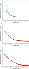 |
Fig. 9. Evolution of noise spectra over the mission lifetime for radiometer 18M (70 GHz, top), 25S (44 GHz, middle), and 27M (30 GHz, bottom). Spectra are colour-coded, ranging from OD 100 (blue) to OD 1526 (red), with intervals of about 20 ODs. White-noise levels and slope stability are considerably better than in the 2015 release, being at the 0.1% level for noise, while knee-frequencies show variations at the 1.5% level. |
White-noise levels for the LFI radio meters.
Knee frequencies and slopes for each of the LFI radiometers.
6. Mapmaking
The methods and implementation of the LFI mapmaking pipeline are described in detail in Planck Collaboration II (2016), Planck Collaboration VI (2016), and Keihänen et al. (2010). Here we report only the changes introduced into the code with respect to the previous release.
Our pipeline still uses the Madam destriping code, in which the correlated noise component is modelled as a sequence of short baselines (offsets) that are determined via a maximum-likelihood approach. In the current release, the most important change is in the definition of the noise filter in connection with horn-uniform detector weighting. When combining data from several detectors, we assign each detector a weight that is proportional to
 (7)
(7)
where  and
and  are the white-noise variances of the two radiometers (“Main” and “Side”) of the same horn. The same weight is applied to both radiometers. In the 2015 release the weighting was allowed to affect the noise filter as well: for the noise variance σ2 in Eq. (6) we used the average value Cw. For the current release we have completely separated detector weighting from noise filtering. We use the individual variances
  and
and  for each radiometer when building the noise filter. In principle, this makes maximum use of the information we have about the noise of each radiometer.
We compared the previous and the current versions of Madam, using a single noise filter, and found excellent agreement. Differences were at the 0.01 μK level, and the code took the same number of iterations. We then compared the results obtained with the combined noise filter with those obtained with the separated noise filters for each radiometer. We found that using separate filters for the two radiometers of the same horn has the effect of reducing the total number of iterations required for convergence by almost a factor of 2. The net effect of using both the new version of Madam and the separate noise filters is that we obtain the same maps as before, but considerably faster.
In Figs. 10–12, we show the 30-, 44-, and 70 GHz frequency maps. The top panels are the temperature (I) maps based on the full observation period, and presented at the original native instrument resolution, HEALPixNside = 1024. The middle and bottom panels show the Q and U polarization components, respectively; these are smoothed to 1 deg angular resolution and downgraded to Nside = 256. Polarization components have been corrected for bandpass leakage (see Sect. 7). Table 6 gives the main mapmaking parameters used in map production. All values are the same as for the previous data release except the monopole term; although we used the same plane-parallel model for the Galactic emission as for the 2015 data release, the derived monopole terms are slightly changed at 30 and 44 GHz for the adopted calibration procedure.
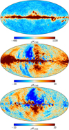 |
Fig. 10. LFI maps at 30 GHz: top: total intensity I; middle: Q polarization component; bottom: U polarization component. Stokes I is shown at instrument resolution and at Nside = 1024, while Q and U are smoothed to 1° resolution and at Nside = 256. Units are μKCMB. The polarization components have been corrected for bandpass leakage (Sect. 7). |
Mapmaking parameters used in the production of maps.
7. Polarization: Leakage maps and bandpass correction
The small amplitude of the CMB polarized signal requires careful handling because of systematic effects capable of biasing polarization results. The dominant one is the leakage of unpolarized emission into polarization; any difference in bandpass between the two arms of an LFI radiometer will result in such leakage. In the case of the CMB, this is not a problem. That is because calibration of each radiometer uses the CMB dipole, which has the same frequency spectrum as the CMB itself, and so exact gain calibration perfectly cancels out in polarization. However, unpolarized foreground-emission components with spectra different from the CMB will appear with different amplitudes in the two arms, producing a leakage into polarizaion.
In order to derive a correction for this bandpass mismatch, we exploit the IQUSS approach (Page et al. 2007) used in the 2015 release. The main ingredients in the bandpass mismatch recipe are the leakage maps L, the spurious maps Sk (see below), the a-factors, and the AQ[U] maps (see Sect. 11 of Planck Collaboration II 2016, for definitions). With respect to the treatment of bandpass mismatch in the previous release, we introduce three main improvements in the computation of the L and A maps. Leakage maps, L, are the astrophysical leakage term encoding our knowledge of foreground amplitude and spectral index. These maps are derived from the output of the Commander component-separation code. In the present analysis this is done using only Planck data from the current data release at their full instrumental resolution. In contrast, in the earlier approach we also used WMAP 9-year data and applied a 1 deg smoothing prior to the component-separation process. We also exclude Planck channels at 100 and 217 GHz, since these could be contaminated by CO line emission. Spurious maps Sk (one for each radiometer) are computed from Madam mapmaking outputs (for the full frequency map creation run). Basically, spurious maps are proportional to the bandpass mismatch of each radiometer, and can be computed directly from single radiometer timelines. As described in Planck Collaboration II (2016), the output of the Main and Side arms of a radiometer can be redefined, including bandpass mismatch spurious terms, as
 (8)
(8)
or in the more compact form
 (9)
(9)
Here α1 and α2 can take the values −1, 0, and 1. The problem of estimating m = [I, Q, U, S1, S2] is similar to a mapmaking problem, with two extra maps. The pixel-noise covariance matrix is therefore given by the already available Madam-derived covariance matrix, with two additional rows and columns, as
 (10)
(10)
The Planck scanning strategy allows only a limited range of radiometer orientations. We therefore compute a joint solution with all radiometers at each frequency that helps also to reduce the noise in the final solutions. Once spurious maps are derived, we compute the a-factors from a χ2 fit between the leakage map L and the spurious maps Sk on those pixels close to the Galactic plane, |b|< 15° (at higher latitudes both foregrounds and spurious signals are weak and do not add useful information).
The last improvement involves the final step in the creation of the correction maps. Recall that polarization data from a single radiometer probe only one Stokes parameter in the reference frame tied to that specific feedhorn. This reference frame is then projected onto the sky according to the actual orientation of the spacecraft, which modulates the spurious signal of each radiometer into Q and U. This modulation can be obtained by scanning the estimated spurious maps  , to create a timeline that is finally reprojected into a map. In the previous release, instead of creating timelines and then maps (a time- and resource-consuming operation) we built projection maps AQ[U] that accounted exactly for horn and radiometer orientation. The final correction maps were
![Mathematical equation: $$ \begin{aligned} \Delta Q[U] = L\times \sum _k a_k A_{k,Q[U]}\, , \end{aligned} $$](/articles/aa/full_html/2020/09/aa33293-18/aa33293-18-eq121.gif) (11)
(11)
where ak and Ak, Q[U] are the a-factors and the projection map for the radiometer k of a given frequency. In using this approach, however, there were two drawbacks. The first and more important one is related to a monopole term present in the leakage map L that directly impacted the correction maps. The synchrotron component, in fact, has a significant quasi-isotropic component (perhaps related to the ARCADE2-measured excess; Fixsen et al. 2011) and this contributed exactly to a monopole term in the correction map. Q and U maps, however, are produced by Madam, which tends to remove any possible monopole term. Therefore, with the simple approach of Eq. (11), we transfered the monopole term into the correction, and hence into the final bandpass-corrected map, resulting in an overestimation of the actual real effect. This was negligible at 70 GHz, but important in the 30 GHz map, which is used to correct foregrounds in the 70 GHz likelihood power spectrum estimation. The second drawback was that the resulting correction maps displayed sharp features, especially around the ecliptic poles. These were intrinsic to the projection maps, and caused problems with nearby point sources.
To resolve these issues, given new computing resources available, we exploit the scanning, timeline creation, and mapmaking approach. This is done using the Planck LevelS simulation package (Reinecke et al. 2006), which takes the harmonic coefficients aℓ m of the leakage maps, multiplied by the derived a-factors, and the actual scanning strategy, and then creates timelines accounting for proper beam convolution as well. The resulting TOD are used to create maps with the Madam mapmaking code. It is clear that in this way the final correction map is processed by the same mapmaking used for official map production and hence removes the presence of unwanted monopoles. In addition, accounting for beam convolution significantly alleviates the presence of sharp features in the correction maps.
Table 7 gives the estimated a-factors for the current release. They are very close to the 2015 values at 30 and 44 GHz, with larger (but within 1σ) variations at 70 GHz. We investigated the origin of these variations by computing the a-factors with the present data, but using the old version of the leakage map. We find results in agreement with those obtained before. We also performed the same analysis with old data but with the new version of the leakage maps. In this case, we find results in line with the current estimates. These very simple tests clearly indicate that the observed variations in the a-factors are not due to the adopted calibration pipeline, but are mainly due to the changes in the leakage maps derived using Planck data only and excluding CO-dominated HFI channels.
Bandpass mismatch a-factors from a fit to Sk = akL.
8. Data validation
We verify the LFI data quality with the same suite of null tests used in previous releases and described in Planck Collaboration II (2016). As before, null tests cover different timescales (pointing periods, surveys, survey combinations, and years) and data (radiometers, horns, horn-pairs, and frequencies) for both total intensity and polarization. These allow us to highlight possible residuals of different systematic effects still present in the final data products.
8.1. Comparison between 2015 and 2018 frequency maps
Before presenting the null-test results, we compare the 2015 and 2018 maps. We expect improvements especially at 30 and 44 GHz, where the calibration procedure is significantly changed. Figure 13 shows differences between 2018 and 2015 frequency maps in I, Q, and U. Large scale differences between the two set of maps are mainly due to changes in the calibration procedure, but the exact origin of the differences is not revealed by these overall frequency maps.
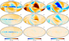 |
Fig. 13. Differences between 2018 (PR3) and 2015 (PR2) frequency maps in I, Q, and U. Maps are smoothed to 1° angular resolution for I and to 3° for Q and U, in order to highlight large-scale features. Differences are clearly evident at 30 and 44 GHz, and are mainly due to changes in the calibration procedure. |
A clearer indication of the origin of improvements in 2018 is given by survey differences at the frequency map level in temperature and polarization. From results for the previous release, we know that odd minus even surveys are the most problematic because of the low dipole signal in even numbered Surveys (especially in Surveys 2 and 4), which increases calibration uncertainty. This indeed was the motivation for the changes made in the calibration pipeline. In addition, since the optical coupling of the satellite with the sky is reversed every 6 months, such survey differences are the most sensitive to residual contamination from far sidelobes not properly accounted for and subtracted during the calibration process. We therefore consider the set of odd-even survey differences combining all eight sky surveys covered by LFI. These survey combinations optimize the signal-to-noise ratio, and are shown in Fig. 14 with a low-pass filter to highlight large-scale structures. The nine maps at the top show odd-even survey differences for the 2015 release, while the nine maps at the bottom show the same for the 2018 release.
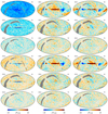 |
Fig. 14. Differences between odd (i.e., Surveys 1, 3, 5, and 7) and even (Surveys 2, 4, 6, and 8) surveys in I, Q, and U (from left to right) for the 2015 (upper nine maps) and 2018 (lower nine maps) data releases. These maps are smoothed to 3 deg to reveal large-scale structures. |
The 2015 data show large residuals in I at 30 and 44 GHz that bias the difference away from zero. This effect is considerably reduced in the 2018 release, as expected from the improvements in the calibration process. The I map at 70 GHz also shows a significant improvement. In the polarization maps, there is a general reduction in the amplitude of structures close to the Galactic plane: the Galactic centre region and the bottom-right structure in Q at 30 GHz, and the rightmost region on the Galactic plane in U.
Figure 15 shows pseudo-angular power spectra from the odd-even survey differences, using the same sky mask as for the null-test spectra in Sect. 8.2, namely the union of all the single survey masks. There is great improvement in 2018 in removing large-scale structures at 30 GHz in TT, EE, and somewhat in BB, and also in TT at 44 GHz. These improvements are again expected and the reason is two-fold. First, the improved calibration now allows better tracing of the actual instrument gain, even in the low-dipole-signal period, both for 30 and 44 GHz. Second, the improved calibration enhances our ability to remove far-sidelobe contamination, resulting in significantly cleaner 30 GHz maps. At 70 GHz, even though the calibration procedure is almost unchanged from the 2015 release, we are able to reduce large-scale residuals in TT, thanks to the combined effect of data selection and the gain smoothing algorithm.
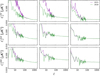 |
Fig. 15. Angular pseudo-power spectra of the odd-even survey difference maps for 30 (left column), 44 (middle column), and 70 GHz (right column), with the 2015 data in purple and 2018 in green. |
8.2. Null-test results
These findings are confirmed by specific null tests, taking differences of frequency maps for odd and even surveys. As for the previous release, we present differences among the first three sky surveys. Figure 16 shows the total amplitude of the polarized signal at 30 GHz (the channel with the largest expected differences), smoothed with an 8 deg Gaussian beam. Odd-even Survey differences reveal clear structures on large angular scales that are significantly reduced in the 2018 data set. In contrast, the Survey 1 versus Survey 3 difference map shows no large-scale features. This is expected, since for both Surveys 1 and 3 the dipole signal used for calibration is large. Moreover, the far sidelobes are orientated similarly with respect to the sky for these two surveys.
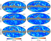 |
Fig. 16. Survey difference maps of polarization amplitude at 30 GHz for the current 2018 (right) and 2015 (left) releases. The improvement is evident, especially in odd-even difference maps, showing lower residuals due to the new calibration approach. Maps are smoothed with an 8 deg Gaussian beam to show large-scale structures. |
We also inspect angular power spectra of odd-even survey differences, adopting as a figure of merit the noise level derived from the “half-ring” difference maps (made from the first and second half of each stable pointing period) weighted by the hit count. This quantity traces the instrument noise, but filters away any component fluctuating on timescales longer than the pointing period. To illustrate the general trend in null tests and the improvements in the 2018 release, Fig. 17 shows TT and EE Survey-difference power spectra for the 2015 and 2018 data sets. We compare these spectra with noise levels derived from the corresponding half-ring maps.
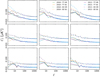 |
Fig. 17. Null-test results comparing power spectra from survey differences to those from the half-ring maps. Differences are: left: Survey 1 − Survey 2; middle: Survey 1 − Survey 3; and right: Survey 1 − Survey 4. These are for 30 GHz (top), 44 GHz (middle), and 70 GHz (bottom), for both TT and EE power spectra. There is a significant improvement in Survey 1 − Survey 2 and Survey 1 − Survey 4 at 30 GHz, especially in EE. |
Results at 30 and 44 GHz are in line with expectations. In particular we see improvements at 30 GHz (survey differences are close to half-ring spectra) when considering odd-even survey differences. The better agreement results from the improved treatment of residual polarization by iterating Galactic modelling during calibration. The 44- and 70 GHz results are basically in line with the previous release findings. That is of course expected at 70 GHz, since the calibration procedure is almost the same as in the previous release, except for the gain smoothing algorithm and the foreground model adopted (now based on the Commander solutions using only Planck data).
A more quantitative way to represent null-test results, especially at low multipoles, is to compute deviations from the half-ring noise in terms of
 (12)
(12)
We specifically sum each single  in the range ℓ = 2–50. Then, from the total value of χ2 and Ndof, we derive p-values of the distribution. While a proper set of noise simulations should in principle be considered, for this inspection it is adequate to use simple half-ring noise. Nonetheless we should be aware of the fact that any result derived with this approach is only indicative of possible issues and that a more detailed and refined analysis is required. Table 8 reports both χ2 and p-values from the three survey differences, as shown in Fig. 17 for polarization spectra at the three LFI frequencies for the 2018 and 2015 data releases. A comment is in order here. On the one hand, we see that Survey 2 and Survey 4 seem to have some problems at 70 GHz, as highlighted by the poor χ2 and p-values. However, this is expected, since we made only relatively small changes in the calibration pipeline at 70 GHz, and these surveys were known to be problematic in 2015. Nevertheless, we can anticipate that a power spectrum analysis of low-ℓ polarization at 70 GHz will find good results even including Survey 2 and Survey 4, thanks to the use of the calibration template described in Sect. 3. We note, however, that such a template does not help to improve the χ2 and p-values, since these are derived from survey differences; any global template applied to data from both surveys would cancel out and leave χ2 results unaffected. While at 44 GHz the picture is practically unchanged with respect to 2015, results at 30 GHz show in general a good trend of improvement for even survey differences, as indicated by χ2 values, and underlining again the benefit of the new calibration scheme. However, such values are far from being optimal and may indicate the presence of residuals showing up in the difference maps. Moreover we stress that this kind of analysis is only indicative and is used internally as an additional validation test.
Odd-even surveys χ2 and p-values (2 ≤ ℓ ≤ 50).
8.3. Half-ring test
The actual noise in the LFI data is given directly by the half-ring difference maps. Detailed noise characterization is of paramount importance for the creation of adequate noise-covariance matrices (NCVMs), as well as for the noise MC realizations that are required in subsequent steps of the data analysis. Any noise model has to be validated against such half-ring difference maps. In the current release, we follow the same processing steps as in the previous releases. Specifically, we compute anafast auto-spectra in temperature and polarization of the half-ring difference maps for the period covering the full mission. This is also done on MC noise simulations produced using noise estimation at the TOI level taken from FFP103. Half-ring noise power spectra are compared with the distribution of noise spectra derived from the noise simulations and with the white-noise level computed from the white-noise covariance matrices (WNCVM) produced during the mapmaking process.
Figure 18 shows such a comparison for TT, EE, and BB spectra. The grey bands represent the 16% and 84% quantiles of the noise MC, while the black solid line is the median (50% quantile) of these distributions. The half-ring spectra are depicted in red, and for ℓ ≥ 75 are binned over a range of Δℓ = 25. Even by eye the agreement is extremely good, and makes us confident about proper noise characterization in LFI data.
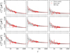 |
Fig. 18. Consistency check at the power spectrum level between half-ring difference maps (red), white-noise covariance matrices (black dash-dotted lines), and 100 full-noise MC simulations (grey band showing range for 16% and 84% quantiles of noise simulations, and the black solid lines giving the median, i.e., 50% quantile, of the distributions). From top to bottom we show TT, EE, and BB power spectra for 30 GHz (left), 44 GHz (centre), and 70 GHz (right). Half-ring spectra are binned with Δℓ = 25 for ℓ ≥ 75. |
We futher investigate the noise properties in the high-ℓ regime, taking the average of 𝒞ℓ in the range 1150 ≤ ℓ ≤ 1800 for both temperature and polarization, and then comparing with the WNCVM. Figure 19 displays the result. As already shown in previous releases, there is still an excess of 1/f noise in this high-ℓ regime, meaning that both the real data and the noise MCs predict slightly larger noise than the WNCVM. It is important to note that such noise excess is reduced considerably with resepct to the 2015 release, thanks mainly to the new and more accurate calibration procedure adopted. Residuals are ≲1.4% at 30 GHz, ≲1% at 44 GHz, and ≲0.6% at 70 GHz, for both temperature and polarization. In addition, agreement between actual noise data and MC simulations is extremely good, with deviations of only fractions of a percent.
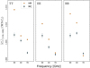 |
Fig. 19. Ratio of mean noise at high multipoles (1150 ≤ ℓ ≤ 1800) to white noise, derived from white-noise covariance matrices produced during the mapmaking process. |
8.4. Intra-frequency consistency check
Data consistency can also be checked by means of power spectra, as done in previous releases (Planck Collaboration II 2016, 2014). We consider frequency maps at 30, 44, and 70 GHz, and take the cross-spectra between half-ring maps at each frequency for the full mission time span. Taking cross-spectra has the advantage that we do not need to consider noise bias at the power spectrum level. We make use of the cROMAster code, a pseudo-Cℓ cross-spectrum estimator (Hivon et al. 2002; Polenta et al. 2005). Results obtained are sub-optimal with respect to a maximum likelihood approach, but are less computationally demanding and accurate enough for our purposes.
The actual spectra are computed using a Galactic mask obtained with the combination of the Planck G040, G060, and G070 masks at 30, 44, and 70 GHz, respectively, and accounting for the proper frequency-dependent masks for resolved point sources. Figure 20 shows cross-spectra from the half-ring maps. They agree well among the three frequencies, which is remarkable since foregrounds have not been removed from the maps, except in the masked regions. The red-dashed lines are the 2015 Planck best-fit TT spectrum, augmented by the contribution from unresolved point sources. The data are in good agreement with this model at all three frequencies. More quantitatively, we build a simple Gaussian likelihood (without any beam or foregrounds modelling) and consider multipole bins up to where the beam function blows up. We obtain the following p-values: 0.196 at 70 GHz (50 ≲ ℓ ≲ 1300); 0.262 at 44 GHz (50 ≲ ℓ ≲ 500); and 0.017 at 30 GHz (50 ≲ ℓ ≲ 500). This shows that even with this simplified approach 70 and 44 GHz are consitent with the model. The 30 GHz channel is marginally consistent with the null hypothesis and clearly requires a more detailed treatment of foregrounds.
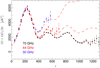 |
Fig. 20. Binned TT cross-spectra from half-ring maps at 30, 44, and 70 GHz. Foregrounds are accounted for only through the use of the proper frequency-dependent Galactic masks. Red-dashed lines are the Planck best-fit TT spectrum, to which a contribution from unresolved point sources (specific to each frequency) has been added. |
As a more quantitative test of data consistency, we build the usual scatter plots of angular power spectra for the three frequency pairs. To ensure a proper comparison, we remove the frequency-dependent contribution from unresolved sources, and perform a linear fit, accounting for errors on both axes. Figure 21 shows results in the multipole range around the first peak, where the effect of different angular resolutions at the three frequencies is still manageable. The agreement is extremely good: spectra are consistent with deviations between 0.9% and 0.1%, a result in line with findings from the previous release (Planck Collaboration II 2016). This agreement is also an indication of the calibration accuracy, which is at the sub-percent level. This is a sign of the good health of our data, given that fact that in these tests we have not accounted for any errors in the window function, calibration, or foreground removal.
 |
Fig. 21. Scatter plots of LFI angular cross-spectra around the first acoustic peak for frequency pairs: left: 70 GHz and 30 GHz; middle: 70 GHz and 44 GHz; right: 44 GHz and 30 GHz. The solid line is the linear fit obtained accounting for error bars on both axes. Slopes, within expected uncertainty, show good consistency among data sets |
8.5. Internal consistency check
We also check the internal consistency of the 70 GHz data used for the cosmological analysis. As done for the 2015 release, we create cross-spectra by taking different data splits. Specifically, we consider the half-ring maps and the year combination maps Year 1−Year 3 and Year 2−Year 4 maps. Figure 22 shows the residuals of the combination, compared with the expectations derived from FFP10 Monte Carlo simulations subjected to the same procedure. Residuals are clearly compatible with the null hypothesis.
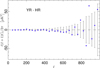 |
Fig. 22. Residuals between cross-spectra at 70 GHz from half-ring (HR) and year maps (YR). Error bars come from FFP10 Monte Carlo simulations. |
To quantify the agreement we apply the Hausman test (Polenta et al. 2005) to 70 GHz cross-spectra from half-ring and year maps. As reported in Planck Collaboration II (2016) we define the statistic
![Mathematical equation: $$ \begin{aligned} H_\ell = \left(\hat{C}_\ell - \bar{C}_\ell \right)\bigg /\sqrt{{\mathrm{Var} }\left[\hat{C}_\ell - \bar{C}_\ell \right]}, \end{aligned} $$](/articles/aa/full_html/2020/09/aa33293-18/aa33293-18-eq124.gif) (13)
(13)
where  and
and  represent the two different cross-spectra. We further compress the multipole information with
![Mathematical equation: $$ \begin{aligned} B_L(r) = \frac{1}{\sqrt{L}}\sum _{\ell =2}^{\left[Lr\right]}H_\ell ,\,\, r\in [0,1], \end{aligned} $$](/articles/aa/full_html/2020/09/aa33293-18/aa33293-18-eq127.gif) (14)
(14)
where the operator [.] returns the integer part. It can be shown that the distribution of BL(r) converges to Brownian motion, which can be simply studied by means of three statistics: s1 = sup BL(r); s2 = sup|BL(r)|; and  . Results are reported in Fig. 23, where the three statistics are compared to their expected distributions derived from FFP10 simulations. The corresponding p-values for s1, s2, and s3 are, respectively, 0.11, 0.19 and 0.13, showing again that results are perfectly compatible with the null hypothesis, and confirming the high level of internal consistency in the 70 GHz data.
 |
Fig. 23. Empirical distributions derived from FFP10 simulations for the s1, s2, and s3 statistics of the Hausman test on the 70 GHz data. Vertical lines show values derived from half-ring and year maps at 70 GHz. |
8.6. Validation summary
At the end of this detailed validation process, the improved quality of the 2018 data release, especially at 30 and 44 GHz, is clear. This improvement is mainly due to the new calibration procedure implemented. It is also evident that residuals at very low multipoles (large angular scales) are still present at 30 and at 44 GHz. One of the reasons could be the fact that the initial foreground model used for the iterative calibration, mapmaking and component-separation process was entirely based on LFI data. We took this approach to avoid dependence on WMAP and to avoid ingesting any HFI systematic effects. However, we realize that this results in a foreground model with less power than expected. This choice should in principle be investigated further, but the actual level of residuals is small and does not prevent the use of the 30 GHz data as a synchrotron template in cosmological analyses involving the 70 GHz LFI channel (see Planck Collaboration V 2020, for a detailed analysis of the low-ℓ likelihood.).
9. Updated systematic effects assessment
9.1. General approach
Analysis of LFI systematic effects from the start of the mission to the 2015 release (Planck Collaboration III 2014; Planck Collaboration II 2016; Planck Collaboration III 2016) identified uncertainty in calibration as the dominant source of systematic error. This source of error, and all other known systematic effects, are at least four orders of magnitude below the measured CMB power spectrum in total intensity for all relevant multipoles (see Figs. 24–26 of Planck Collaboration III 2016). However, this is not the case for polarization. Imperfect gain reconstruction, obtained independently for the Main and Side radiometers of each horn, translates directly into leakage of total intensity to polarization. In particular, at the large angular scales relevant for probing the reionization bump, the systematic error from calibration is comparable with the expected signal, for reasonable values of the optical depth parameter τ.
Our assessment of the overall systematic error budget remains essentially unchanged from the 2015 release, as summarized in Table 1 of Planck Collaboration III (2016) and references therein. For the present release, we have concentrated on developing a detailed simulation programme to model all known instrumental and astrophysical effects that produce uncertainty in the gain for polarization data. We first identify those parameters in the whole calibration process that are affected by uncertainties, and then set up an ad hoc Monte Carlo simulation strategy to judge the effect of varying these parameters. This process has to be both accurate and realistic. There are two possible sources of error that are quite different in nature: statistical uncertainties, related to instrumental noise in conjunction with variations in the dipole amplitude on the sky; and systematic uncertainties due to effects and assumptions in the calibration process that are not completely known. The simulations require a trade-off between a full, physically representative set of simulations and a realistic, feasible number of simulations, given the computation resources available. Ideally, we would assume that all the effects are indeed correlated with each other, and therefore the total number of simulations would be the product of the number of simulations required for each single effect. However, to reduce computer resources needed, it is more convenient to assume that all the effects are un-correlated, and the final error is obtained by summing in quadrature the error derived from each single effect. This uncorrelated assumption is clearly not completely true: it is impossible to separate the effect of different parameter values of the gain smoothing algorithm from the actual noise realization. Therefore, we follow a hybrid approach in the systematic effect simulations.
9.2. Monte Carlo of systematic effects
The FFP10 (see Planck Collaboration X 2016) simulation pipeline is the basis of our simulations pipeline, and the sky signal we include makes use of the Planck Sky Model (Delabrouille et al. 2013). A detailed description of the sky model and components is given in Appendix B. In the current implementation, the FFP10 pipeline is partially executed in full timelines (data as a function of time at the original detector sampling frequency), and partially in the ring-set domain (data binned into a partial map for every pointing period covering full circles on the sky, as identified by HEALPix pixel indices).
We start by creating separate ring-sets for each signal of interest, using the actual pointing information. We have ring-sets for CMB, Galactic foregrounds, extragalactic diffuse signals, point sources convolved with the measured LFI beams, and finally the sum of the solar and orbital dipoles, also convolved with the measured LFI beams. In the second stage of the pipeline, we perform the iterative calibration. First we divide ring-sets by a fiducial set of gains (those estimated from actual data), and then we process ring-sets to estimate the gain value for each pointing period using the same pipeline as described (although using a different implementation) in Planck Collaboration V (2016). The reconstructed gains, however, are noisy and biased when the orientation of the line of sight of the telescope scans a region where the dipole is close to its minimum. Therefore we apply the same smoothing algorithm developed by the DPC for the real data. It is important to note here that the smoothing algorithm is optimized through a detailed study of real data, and we therefore do not expect that it will perform optimally on each single simulation. Observed differences in the final maps could be used to estimated directly the impact of the smoothing process on the reconstructed gains.
The final stage of simulations produces calibrated maps with a pipeline based on TOAST4. We combine timelines of the desired input signals and noise (exactly the same as already used to create ring-sets for the calibration process), and divide by the fiducial gains, converted into kelvin with the previously computed set of reconstructed gains. From these calibrated timelines we subtract the simulated dipole signal, and then create maps with Madam. Any discrepancy between the fiducial and reconstructed gains shows up as a residual dipole and a mis-calibration of the Galactic signal and the noise. This gives an estimate of the calibration error that we believe also affects the data.
We have also examined in more depth the impact of known systematic effects on the calibration process, using targeted simulations. These simulations include noiseless maps for a few different realizations of each individual systematic effect: different solar dipole amplitudes and directions based on the expected error on the Planck dipole; different masks used inside the calibration pipeline during the gain fitting process; different beams used to convolve foreground signal and dipoles, based on the expected error on bandpasses and its impact on beams; ADC nonlinearities, based on the model fitted to real data; and finally different sky signals for input and calibrator, in order to simulate a discrepancy between input data and our sky model. We create simulations of each single effect plus a set of 20 simulations that include many different effects together by randomly sampling all the available options from dipole, beam, and ADC systematics, plus realistic noise simulations. It should be clear from this description that we are following a hybrid approach where, although simulated independently, systematic effects can be combined together to produce a new set of gains and maps.
In the following paragraph we describe results from these simulations of systematic effects. There are two outcomes. First, the results show how well we are able to simulate instrumental and data-processing effects in a direct comparison (mainly at power spectra level) with null tests on the data. Second, they provide a quantitative estimation of the amplitude of systematic effects. We will also summarize the overall systematic error budget, accounting for effects not directly simulated in 2018 by using simulations performed for the 2015 data release. In the evaluation of the various effects, we also used a perfect calibration simulation, where the pipeline is exactly the same except that we use the same set of fiducial gains in both the de-calibration and calibration processes.
9.2.1. Gain smoothing error
One of the most delicate steps in the calibration pipeline is the smoothing of the raw gains obtained from the dipole/sky fitting procedure. The smoothing algorithm is described in detail in Planck Collaboration V (2016), and has been tailored to the LFI data. Its performance is strictly linked to the actual noise in the data, the level of dipole signal with respect to the sky signal, and the contribution of the far-sidelobe pickup. An algorithm tuned to the specifics of the real data might not perform equally well on any single simulation, and one might be tempted to optimize the smoothing procedure for each one. We choose not to do that, both because it would be a lengthly process, and also because it would introduce the gain smoothing algorithm itself as a new variable that would vary among simulations, making a direct comparison much more cumbersome. Instead using exactly the same smoothing procedure applied to real data allows us to evaluate its impact on data when compared to a perfect calibration simulation.
Figure 24 compares angular power spectra of odd-even-year null tests (in other words, the difference between the sum of Year 1 and Year 3 and the sum of Year 2 and Year 4) with the distribution (median plus 16% and 84% quantiles) derived from simulations. The simulations include the impact of the gain smoothing algorithm on the gain set that has been derived using the full set of systematic simulations, but applied to the noise-only timestream. We see that there is overall good agreement between data null tests and these pure-noise simulations. However, there are clearly some multipoles for which data null values are outside the range of simulations. This tells us that there are effects in the data other than the gain smoothing error. Indeed, we made the same comparison for perfect calibration simulations, and found a very similar plot with very small differences in the distribution of simulated spectra. In order to evaluate the impact of the gain smoothing error, we take the amplitude (for both perfect calibration and gain smoothing error) of the 1σ bands for some specific range of multipoles. Considering ℓ = 4–5, the overall effect of the gain smoothing algorithm for the three frequency channels is to increase noise by ≲3 × 10⁻³ μK2 in total intensity and ≲6 × 10⁻³ μK2 in polarization, almost the same for all three frequencies. Considering higher multipole ranges, ℓ ≃ 100 and ℓ ≃ 500, errors are reduced by at least one order of magnitude with respect to the ℓ = 4–5 range, ranging between 10−4–10−5 μK2, both in temperature and polarization.
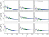 |
Fig. 24. Odd-even-year null spectra compared with simulations including the gain smoothing algorithm at 30 (left), 44 (middle), and 70 GHz (right). The pink band shows the 16%–84% quantile range of the simulations, with the median traced by the blue line. On large angular scales the data show larger variations with multipole than the simulations. |
9.2.2. ADC nonlinearities
The ADCs convert analogue detector outputs into numbers, and any nonlinearities in their response could mimic a sky signal thereby affecting data calibration. As mentioned in Sect. 2, for the current release we implemented a new method to track and correct ADC nonlinearities that improves the quality of the data at 30 GHz.
As well as the analysis done in the definition of the new correction method, we also performed specific simulations of the effects of nonlinearities in the ADCs. We created 10 noiseless simulations with the ADC effect, based on a model fitted with real data. In these simulations, we randomized the errors in the voltage steps associated with each binary bit of the ADC in a way that is consistent with what we found from the data. Results are in line with the findings in 2015, with improvements at 30 GHz where residuals decrease by almost an order of magnitude. Again considering the range ℓ = 4–5, the ADC effects now contribute an increase in the noise of ≲10−4 μK2 at 30 GHz and around 10−5 μK2 at 44 and 70 GHz. At higher multipoles the effect drops below 10−6 μK2. In polarization the effect is at least one order of magnitude smaller than in total intensity.
9.2.3. Full systematic simulations
The final set of simulations we consider includes all the effects that we expect to directly impact calibration accuracy. We now present the results obtained, together with a final comprehensive table of the estimated impact of systematic effects. In addition, we create a summary plot like the ones in Planck Collaboration III (2016), but with updates for those effects being simulated for the current data release, including plots of EE and BB.
We begin by comparing the full systematic error budgets between the current and the 2015 data release. Figure 25 shows TT and EE angular power spectra at the three LFI frequencies. Systematic simulations made for the two data releases are in very good agreement; this justifies our claim that the overall systematic error budget remains essentially unchanged between 2015 and 2018. Moreover, the null spectra from odd-even-year differences are very close to the systematic error expectations, both in temperature and polarization. There are a very few multipoles where null spectra lie outside the 1σ band of the simulations. Specifically, for TT they are ℓ = 2 and 3 at 30 GHz, and ℓ = 2 for both 44 and 70 GHz. The extra variance in the null tests is ≲0.04 μK2 at 30 and 70 GHz, and around 0.065 μK2 at 44 GHz. At higher multipoles, the agreement with simulations, dominated by instrumental noise, is extremely good.
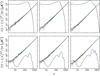 |
Fig. 25. Angular TT (top) and EE (bottom) power spectra at 30 (left), 44 (middle), and 70 GHz (right) of a complete set of systematic effects for the 2015 data release (red) and the 2018 simulations (blue, 50% percentile plus 1σ band from simulations). This shows the good agreement between the two releases. In green we show the null spectra from odd-even year difference. The CMB angular power spectra (black lines) are convolved with the frequency dependent window functions. |
For the EE power spectra, we can see again very good agreement between systematic simulations performed for the 2015 data release and those done for the current release. We see that the overall account of systematics estimated in 2015 falls very close to the median of the present simulations and, in any case, well within the 1σ limits. In addition, the odd-even-year null difference is extremely well represented by our simulations, except at a few multipoles. This again tells us that we understand well the instrumental and systematic effects actually present in the data. Evaluating the extra variance in the data not accounted for by simulations, we see that at 30 GHz the agreement is extremely good, at 44 GHz, there is an excess at ℓ = 4–6 of ≲0.05 μK2, while at 70 GHz, the very low multipoles are in line with expectations (although for ℓ = 10 there is an excess of about 0.10 μK2).
Table 9 summarizes systematic effects at the power spectrum level for three multipole ranges: ℓ = 4–5; around the CMB first peak ℓ ≃ 100; and the almost noise-dominated regime ℓ ≃ 500.
Additional noise in μK2 from systematic effects for three different multipole ranges (ℓ = 4–5, ℓ ≃ 100, and ℓ ≃ 500).
A comment is in order here: for multipoles ℓ ≳ 100, it is clear that the extra noise induced by systematic effects is well described by simulations, and accounted for in the overall estimation of the noise budget. At large angular scales, the improvement with the new calibration scheme is evident from the comparison of null-test spectra on different data combinations between the 2015 and 2018 data releases. However, there are a few multipoles that deserve particular attention, since specific null tests still show a noise excess that is not completely traced by the simulations of systematics. Nevertheless, results presented in this section are intended to be a useful indication of the overall amplitude of systematic effects. More scientifically-oriented analysis could in principle make use of the simulations to build a template that could be fitted for in a maximum likelihood approach (along the same lines as foreground emission templates), and where errors in the simulations could be properly propagated into the final low-ℓ angular power spectrum and cosmological parameters.
10. LFI data products available through the Planck Legacy Archive
Before concluding, we provide a list and short description of the Planck LFI data products available through the Planck Legacy Archive5, based on the data covering the operational lifetime of the instrument from 12 August 2009 to 23 October 2013 (for further details on the data format refer to the Explanatory Supplement, Planck Collaboration 2018).
-
Pointing timelines: identical to the 2015 release. One FITS file for each OD for each frequency. Each FITS file contains the OBT (on-board time) and the three angles, θ, ϕ, and ψ that identify each sample on the sky.
-
Time timelines: identical to the 2015 release. One FITS file for each operational day (OD) for each frequency. Each FITS file contains the OBT and its corresponding International Atomic Time (TAI) value (without leap second) in modified Julian-day format. The user can thus cross-correlate OBT with UTC.
-
Housekeeping timelines: identical to the 2015 release. All housekeeping parameters with their raw and calibrated values, separated by the housekeeping sources, for each OD.
-
Timelines in volts: raw scientific data in volts for each detector at 30, 44, and 70 GHz, and each OD, before any calibration procedure and with no instrumental systematic effects removed.
-
Cleaned and calibrated timelines: provided in KCMB units, for each detector at 30, 44, and 70 GHz, and each OD, after scientific calibration and with convolved dipoles and convolved Galactic straylight removed.
-
Scanning beam: 4π beam used in the calibration pipeline.
-
Effective beam: sky beam representation as a projection of scanning beam on the maps.
-
Full-sky maps at each frequency: maps of the observed sky at 30, 44, and 70 GHz in temperature and polarization at Nside = 1024, and also at Nnside = 2048 for 70 GHz. Maps are delivered for different data periods. We note that the Planck adopted polarization convention is not the one proposed by “IAU” but the one used more generally in CMB full-sky maps and referred to as “COSMO” (see Planck Collaboration 2018).
-
Bandpass correction maps at each frequency and maps with the bandpass correction applied to delivered frequency sky maps (one specific example of each different data period) computed according to the prescription detailed in Sect. 7.
-
Gain Correction Template: template map to be subtracted from the delivered full sky map at 70 GHz in order to account for calibration uncertainties. This template has to be removed prior of any cosmological exploitation of the 70 GHz map. For completeness we also deliver the 70 GHz map with both bandpass and gain correction template applied.
-
RIMO (Reduced Instrument MOdel): model which includes parameters for the main instrument properties, including noise, bandpass, and beam function.
11. Discussion and conclusions
We have presented a comprehensive description of the LFI data analysis pipeline that produces final frequency maps to be used for scientific exploitation. The major improvements with respect to the 2015 data release are in the new iterative calibration procedure at 30 and 44 GHz, which uses sky estimation and component separation to create a sky model to be fed into the calibration algorithm. Other minor improvements are in the re-definition of the data flags that allow better selection of data.
The validation and improvements of the current data release are performed with the usual battery of null tests on data with different observing periods (half-rings, odd-even survey differences, odd-even year differences). In addition, we performed an exhaustive comparison of the results on such null tests obtained with the 2015 and 2018 data sets. These tests, more than any others, clearly show the improvements in the data quality, especially at 30 and 44 GHz, thanks to the new calibration scheme. The better data selection in 2018 is also able to marginally improve the quality of the 70 GHz.
For the analysis of systematic effects, we chose here not to consider the whole set of effects simulated in 2015, but select only those expected to contribute to the final calibration accuracy. As a result, the overall systematic error budget remains unchanged with respect to 2015, and we have verified that this assumption is indeed true by comparing present and past simulations with current null test spectra. Specifically, we consider the ADC nonlinearity effect, the impact of the gain smoothing algorithm, and the impact of parameters in both the 4π beams and the direction and amplitude of the solar dipole. The end result is that for multipoles ℓ ≳ 100, the impact of systematic effects is well described by simulations, and is well-accounted for in the overall error budget. At large angular scales there are still a very few multipoles that show a noise excess with respect to simulations. It is important to note that our power spectrum analysis is performed on a masked sky with a pure pseudo-Cℓ approach, which is known to be sub-optimal at very low multipoles. Therefore our analysis should be regarded as an overall indication of the amplitude of systematic effects. The 2018 release includes our end-to-end simulations, which allow those interested in systematic effects to create templates of the various systematics, similar to the gain-correction template described in Sect. 3.2.
In conclusion, we have demonstrated substantial improvement in the calibration of the LFI data over previous releases, achieving an overall calibration accuracy of 0.1–0.2%. We have provided a comprehensive description of the uncertainties, including systematic effects. Additional improvements are still possible, and can be anticipated in the future.
Planck (http://www.esa.int/Planck) is a project of the European Space Agency (ESA) with instruments provided by two scientific consortia funded by ESA member states and let by Principal Investigators from France and Italy, telescope reflectors provided through a collaboration between ESA and a scientific consortium led and funded by Denmark, and additional contributions from NASA (USA).
The solar dipole is the dipole anisotropy in the CMB induced by the motion of the solar System barycentre with respect to the rest frame of the CMB itself. The orbital dipole is the modulation of the solar dipole due to the orbital motion of the spacecraft around the Sun.
This is the latest version of the Full Focal Plane Planck simulations similar to the FFP8 version used for the 2015 releases (see Planck Collaboration X 2016 for futher details).
Time Ordered Astrophysics Scalable Tools, http://hpc4cmb.github.io/toast/, developed by the Computational Cosmology Center C3 at Lawrence Berkeley National Laboratory to handle MPI-based parallel data processing.
Acknowledgments
The Planck Collaboration acknowledges the support of: ESA; CNES and CNRS/INSU-IN2P3-INP (France); ASI, CNR, and INAF (Italy); NASA and DoE (USA); STFC and UKSA (UK); CSIC, MINECO, JA, and RES (Spain); Tekes, AoF, and CSC (Finland); DLR and MPG (Germany); CSA (Canada); DTU Space (Denmark); SER/SSO (Switzerland); RCN (Norway); SFI (Ireland); FCT/MCTES (Portugal); and ERC and PRACE (EU). A description of the Planck Collaboration and a list of its members, indicating which technical or scientific activities they have been involved in, can be found at http://www.cosmos.esa.int/web/planck/. The simulations for systematics assessment used the Extreme Science and Engineering Discovery Environment (XSEDE, Towns et al. 2014), supported by National Science Foundation grant number ACI-1548562, in particular the Comet Supercomputer at the San Diego Supercomputer Center through allocation AST160021: “Monte Carlo simulations for calibration uncertainty of the Planck mission”, PI A. Zonca, CoPI P. Meinhold.
References
- Arnaud, M., Pratt, G. W., Piffaretti, R., et al. 2010, A&A, 517, A92 [NASA ADS] [CrossRef] [EDP Sciences] [Google Scholar]
- Basak, S., Prunet, S., & Benabed, K. 2009, A&A, 508, 53 [NASA ADS] [CrossRef] [EDP Sciences] [Google Scholar]
- Bennett, C. L., Larson, D., Weiland, J. L., et al. 2013, ApJS, 208, 20 [Google Scholar]
- Bersanelli, M., Mandolesi, N., Butler, R. C., et al. 2010, A&A, 520, A4 [NASA ADS] [CrossRef] [EDP Sciences] [Google Scholar]
- Blas, D., Lesgourgues, J., & Tram, T. 2011, J. Cosmol. Astropart. Phys., 7, 034 [Google Scholar]
- Cai, Z.-Y., Lapi, A., Xia, J.-Q., et al. 2013, ApJ, 768, 21 [NASA ADS] [CrossRef] [Google Scholar]
- Dame, T. M., Hartmann, D., & Thaddeus, P. 2001, ApJ, 547, 792 [NASA ADS] [CrossRef] [Google Scholar]
- Delabrouille, J., Melin, J. B., & Bartlett, J. G. 2002, ASP Conf. Ser., 257, 81 [Google Scholar]
- Delabrouille, J., Betoule, M., Melin, J.-B., et al. 2013, A&A, 553, A96 [NASA ADS] [CrossRef] [EDP Sciences] [Google Scholar]
- Dio, E. D., Montanari, F., Lesgourgues, J., & Durrer, R. 2013, J. Cosmol. Astropart. Phys., 11, 044 [Google Scholar]
- Eriksen, H. K., Jewell, J. B., Dickinson, C., et al. 2008, ApJ, 676, 10 [NASA ADS] [CrossRef] [Google Scholar]
- Fixsen, D. J. 2009, ApJ, 707, 916 [Google Scholar]
- Fixsen, D. J., Kogut, A., Levin, S., et al. 2011, ApJ, 734, 5 [NASA ADS] [CrossRef] [Google Scholar]
- Górski, K. M., Hivon, E., Banday, A. J., et al. 2005, ApJ, 622, 759 [NASA ADS] [CrossRef] [Google Scholar]
- Haslam, C. G. T., Salter, C. J., Stoffel, H., & Wilson, W. E. 1982, A&AS, 47, 1 [NASA ADS] [Google Scholar]
- Hivon, E., Górski, K. M., Netterfield, C. B., et al. 2002, ApJ, 567, 2 [NASA ADS] [CrossRef] [Google Scholar]
- Keihänen, E., Kurki-Suonio, H., & Poutanen, T. 2005, MNRAS, 360, 390 [NASA ADS] [CrossRef] [Google Scholar]
- Keihänen, E., Keskitalo, R., Kurki-Suonio, H., Poutanen, T., & Sirviö, A. 2010, A&A, 510, A57 [NASA ADS] [CrossRef] [EDP Sciences] [Google Scholar]
- Maino, D., Burigana, C., Górski, K. M., Mandolesi, N., & Bersanelli, M. 2002, A&A, 387, 356 [NASA ADS] [CrossRef] [EDP Sciences] [Google Scholar]
- Meinhold, P., Leonardi, R., Aja, B., et al. 2009, J. Inst., 4, 2009 [Google Scholar]
- Mennella, A., Bersanelli, M., Butler, R. C., et al. 2010, A&A, 520, A5 [NASA ADS] [CrossRef] [EDP Sciences] [Google Scholar]
- Mennella, A., Butler, R. C., Curto, A., et al. 2011, A&A, 536, A3 [NASA ADS] [CrossRef] [EDP Sciences] [Google Scholar]
- Miville-Deschênes, M.-A., Ysard, N., Lavabre, A., et al. 2008, A&A, 490, 1093 [NASA ADS] [CrossRef] [EDP Sciences] [Google Scholar]
- Mo, H. J., & White, S. D. M. 1996, MNRAS, 282, 347 [NASA ADS] [CrossRef] [Google Scholar]
- Page, L., Hinshaw, G., Komatsu, E., et al. 2007, ApJS, 170, 335 [NASA ADS] [CrossRef] [Google Scholar]
- Planck Collaboration. 2011, The Explanatory Supplement to the Planck Early Release Compact Source Catalogue (ESA) [Google Scholar]
- Planck Collaboration. 2015, The Explanatory Supplement to the 2015 Results (ESA), http://wiki.cosmos.esa.int/planckpla2015 [Google Scholar]
- Planck Collaboration. 2018, The Legacy Explanatory Supplement (ESA), http://wiki.cosmos.esa.int/planck-legacy-archive [Google Scholar]
- Planck Collaboration I. 2011, A&A, 536, A1 [NASA ADS] [CrossRef] [EDP Sciences] [Google Scholar]
- Planck Collaboration II. 2014, A&A, 571, A2 [NASA ADS] [CrossRef] [EDP Sciences] [Google Scholar]
- Planck Collaboration III. 2014, A&A, 571, A3 [NASA ADS] [CrossRef] [EDP Sciences] [Google Scholar]
- Planck Collaboration V. 2014, A&A, 571, A5 [NASA ADS] [CrossRef] [EDP Sciences] [Google Scholar]
- Planck Collaboration XXXI. 2014, A&A, 571, A31 [NASA ADS] [CrossRef] [EDP Sciences] [Google Scholar]
- Planck Collaboration I. 2016, A&A, 594, A1 [NASA ADS] [CrossRef] [EDP Sciences] [Google Scholar]
- Planck Collaboration II. 2016, A&A, 594, A2 [NASA ADS] [CrossRef] [EDP Sciences] [Google Scholar]
- Planck Collaboration III. 2016, A&A, 594, A3 [NASA ADS] [CrossRef] [EDP Sciences] [Google Scholar]
- Planck Collaboration IV. 2016, A&A, 594, A4 [NASA ADS] [CrossRef] [EDP Sciences] [Google Scholar]
- Planck Collaboration V. 2016, A&A, 594, A5 [NASA ADS] [CrossRef] [EDP Sciences] [Google Scholar]
- Planck Collaboration VI. 2016, A&A, 594, A6 [NASA ADS] [CrossRef] [EDP Sciences] [Google Scholar]
- Planck Collaboration X. 2016, A&A, 594, A10 [NASA ADS] [CrossRef] [EDP Sciences] [Google Scholar]
- Planck Collaboration XI. 2016, A&A, 594, A11 [NASA ADS] [CrossRef] [EDP Sciences] [Google Scholar]
- Planck Collaboration XII. 2016, A&A, 594, A12 [NASA ADS] [CrossRef] [EDP Sciences] [Google Scholar]
- Planck Collaboration XIII. 2016, A&A, 594, A13 [NASA ADS] [CrossRef] [EDP Sciences] [Google Scholar]
- Planck Collaboration XXVI. 2016, A&A, 594, A26 [NASA ADS] [CrossRef] [EDP Sciences] [Google Scholar]
- Planck Collaboration I. 2020, A&A, 641, A1 [CrossRef] [EDP Sciences] [Google Scholar]
- Planck Collaboration II. 2020, A&A, 641, A2 [CrossRef] [EDP Sciences] [Google Scholar]
- Planck Collaboration III. 2020, A&A, 641, A3 [NASA ADS] [CrossRef] [EDP Sciences] [Google Scholar]
- Planck Collaboration IV. 2020, A&A, 641, A4 [CrossRef] [EDP Sciences] [Google Scholar]
- Planck Collaboration V. 2020, A&A, 641, A5 [CrossRef] [EDP Sciences] [Google Scholar]
- Planck Collaboration VI. 2020, A&A, 641, A6 [NASA ADS] [CrossRef] [EDP Sciences] [Google Scholar]
- Planck Collaboration VII. 2020, A&A, 641, A7 [CrossRef] [EDP Sciences] [Google Scholar]
- Planck Collaboration VIII. 2020, A&A, 641, A8 [CrossRef] [EDP Sciences] [Google Scholar]
- Planck Collaboration IX. 2020, A&A, 641, A9 [CrossRef] [EDP Sciences] [Google Scholar]
- Planck Collaboration X. 2020, A&A, 641, A10 [CrossRef] [EDP Sciences] [Google Scholar]
- Planck Collaboration XI. 2020, A&A, 641, A11 [CrossRef] [EDP Sciences] [Google Scholar]
- Planck Collaboration XII. 2020, A&A, 641, A12 [CrossRef] [EDP Sciences] [Google Scholar]
- Planck Collaboration Int. XVII. 2014, A&A, 566, A55 [NASA ADS] [CrossRef] [EDP Sciences] [Google Scholar]
- Planck Collaboration Int. XLIV. 2016, A&A, 596, A105 [NASA ADS] [CrossRef] [EDP Sciences] [Google Scholar]
- Planck Collaboration Int. XLVIII. 2016, A&A, 596, A109 [NASA ADS] [CrossRef] [EDP Sciences] [Google Scholar]
- Planck HFI Core Team. 2011a, A&A, 536, A4 [NASA ADS] [CrossRef] [EDP Sciences] [Google Scholar]
- Planck HFI Core Team. 2011b, A&A, 536, A6 [NASA ADS] [CrossRef] [EDP Sciences] [Google Scholar]
- Polenta, G., Marinucci, D., Balbi, A., et al. 2005, J. Cosmol. Astropart. Phys., 11, 1 [NASA ADS] [CrossRef] [Google Scholar]
- Reinecke, M., Dolag, K., Hell, R., Bartelmann, M., & Enßlin, T. A. 2006, A&A, 445, 373 [NASA ADS] [CrossRef] [EDP Sciences] [Google Scholar]
- Remazeilles, M., Delabrouille, J., & Cardoso, J.-F. 2011, MNRAS, 418, 467 [NASA ADS] [CrossRef] [Google Scholar]
- Remazeilles, M., Dickinson, C., Banday, A. J., Bigot-Sazy, M.-A., & Ghosh, T. 2015, MNRAS, 451, 4311 [NASA ADS] [CrossRef] [Google Scholar]
- Tinker, J., Kravtsov, A. V., Klypin, A., et al. 2008, ApJ, 688, 709 [NASA ADS] [CrossRef] [Google Scholar]
- Towns, J., Cockerill, T., Dahan, M., et al. 2014, Comput. Sci. Eng., 16, 62 [CrossRef] [Google Scholar]
- Vansyngel, F., Boulanger, F., Ghosh, T., et al. 2017, A&A, 603, A62 [NASA ADS] [CrossRef] [EDP Sciences] [Google Scholar]
- Wang, L., & Steinhardt, P. J. 1998, ApJ, 508, 483 [NASA ADS] [CrossRef] [Google Scholar]
- Weiland, J. L., Osumi, K., Addison, G. E., et al. 2018, ApJ, 863, 2 [Google Scholar]
- Zacchei, A., Maino, D., Baccigalupi, C., et al. 2011, A&A, 536, A5 [NASA ADS] [CrossRef] [EDP Sciences] [Google Scholar]
Appendix A: Comparison of LFI 30 GHz with WMAP K and Ka bands
In order to provide a further check on systematic effects, we present here a comparison in polarization at large scales between the LFI 30 GHz channel and the K and Ka bands from WMAP (Bennett et al. 2013). As a first step we subtract from the Planck 2015 and 2018 maps the corresponding bandpass corrections. We then filter Planck and WMAP maps with a 10 deg-FWHM Gaussian beam in order to suppress high-frequency noise and highlight the large-scale structures. We rescale the K and Ka bands to the LFI 30 GHz effective frequency, assuming synchrotron emission with a spectral index of −3. Finally, we calculate Q and U differences between the Planck 2015 and 2018 maps and the WMAP maps, as shown in Figs. A.1 and A.2.
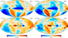 |
Fig. A.1. Stokes Q difference maps between Planck 30 GHz 2015 (top) and 2018 (bottom) and WMAP K-band (left) and Ka-band (right). The WMAP K and Ka band maps are rescaled to match the Planck 30 GHz effective frequency assuming synchrotron emission with a spectral index of −3. All maps used in this comparison have been smoothed with a 10 deg Gaussian beam. |
The amplitude of the large-scale structure in the difference maps decreases by roughly a factor of two between the 2015 and the 2018 maps, reflecting the improvements in the new calibration scheme. This improved calibration has reduced or eliminated some of the features noted by Weiland et al. (2018) in their comparison of WMAP and Planck 2015 Q and U maps. However, as pointed out in Sect. 3.2, the calibration could not be run to convergence for practical reasons, and we expect residuals in the 2018 maps with a pattern similar to that of the 2015 maps. The fact that the difference maps shown in Figs. A.1 and A.2 have some common features with the two Planck releases is therefore not a surprise. There is also some agreement between features in the difference maps and the 70 GHz gain correction template (Fig. 6), which is based in part on the 30 GHz maps. Despite the substantial improvement in the 2018 30 GHz polarization maps, residual systematics are still present, and included in our estimated error budget. Additional improvements are planned in a future paper.
Appendix B: Simulations of systematic effects
B.1. Input Sky Model
The input FFP10 sky includes the following components:
-
Galactic thermal dust, spinning dust, synchrotron, free-free, and CO line emission;
-
the cosmic infrared background;
-
Galactic and extragalactic point sources (radio and infrared);
-
thermal and kinematic Sunyaev Zeldovich effects from Galaxy clusters; and
-
the CMB.
B.1.1. Thermal dust
Galactic thermal dust emission is modelled by scaling across frequencies a polarized template of emission at 353 GHz. The intensity map has been obtained using the Generalized Needlet ILC (GNILC) method of Remazeilles et al. (2011), applied to the 2015 (PR2) release Planck HFI maps, as described in Planck Collaboration Int. XLVIII (2016). The 353 GHz Planck dust map obtained in this way is colour-corrected to obtain a template at 353 GHz. An overall offset of 0.13 MJy sr−1 (corresponding to the residual CIB monopole) is subtracted from the GNILC dust map.
Polarization templates are generated using the prescription of Vansyngel et al. (2017) to generate random dust polarization maps. The method relates the dust polarization sky to the structure of the Galactic magnetic field that is responsible for aligning elongated emitting dust grains, building on the analysis of dust polarization properties described in Planck Collaboration Int. XLIV (2016). The Galactic magnetic field is modelled as a three-dimensional superposition of a mean uniform field and a Gaussian random (turbulent) component with a power-law power spectrum of exponent −2.5. Polarization maps are obtained from the superposition of emission from four emitting layers that all share the same intensity template.
In the vicinity of the Galactic plane, the simulated polarization data are replaced by real Planck 353 GHz data. The transition between real data and simulations is made using a Galactic mask with a 5 deg apodization (which leaves 68% of the sky unmasked), taken from the set of Planck common Galactic masks available in the Planck explanatory supplement6. The first harmonic multipoles, corresponding to ℓ < 10, come from the 353 GHz polarized sky map.
The scaling in frequency of the dust templates uses the prescription used for FFP8. A different modified black-body emission law is used in each of the Nside = 2048 pixels. In addition, the dust spectral index used for scaling in frequency is different at frequencies above and below 353 GHz: for frequency above 353 GHz the modified blackbody parameters obtained in Planck Collaboration Int. XLVIII (2016) are used; below 353 GHz the temperature map is unchanged, but a map of emissivities computed as described in Planck Collaboration Int. XVII (2014) is used instead.
B.1.2. Other Galactic emission
Synchrotron intensity is modelled by scaling in frequency the 408-MHz template map from Haslam et al. (1982), as reprocessed by Remazeilles et al. (2015), using one single power law per pixel. The pixel-dependent spectral index is derived in the analysis of the WMAP data by Miville-Deschênes et al. (2008). The generation of synchrotron polarization follows the prescription of the original PSM paper (Delabrouille et al. 2013).
Free-free, spinning dust models, and Galactic CO emission are essentially the same as used for FFP8 simulations (Planck Collaboration XII 2016), but the actual synchrotron and free-free maps used for FFP10 are obtained with a different realization of small-scale fluctuations of the intensity. CO maps do not include small-scale fluctuations, and are generated from the spectroscopic survey of Dame et al. (2001). None of these three components is polarized in the FFP10 simulations.
B.1.3. Cosmological parameters
The generation of all extragalactic components in the FFP10 sky depends on the assumed cosmological scenario, and in particular values for all cosmological parameters that impact the CMB power spectra (see Planck Collaboration XIII 2016) and/or the statistical distribution of extragalactic objects. We use the parameter values listed in Table B.1, which are used as inputs to the Cosmic Linear Anisotropy Solving System (CLASS) code (Blas et al. 2011; Dio et al. 2013) for generating CMB TT, EE, BB and lensing Φ power spectra, as well as density-contrast shells in auto- and cross-spectra at a set of redshifts (used to model CIB emission). We assume 2.0328 massless neutrinos, and one massive neutrino with a mass of 60 meV, compatible with a standard neutrino hierarchy. The pivot scale for the scalar perturbations is 0.002, and the tensor spectral index and the running of the scalar spectral index are zero.
Cosmological parameters adopted in the PSM.
B.1.4. CMB
The CMB is a stationary Gaussian random field on the sphere, generated from CLASS output power spectra using the HEALPix package, and lensed using the Ilens software of Basak et al. (2009). The joint generation of density contrast shells used for the CIB simulation and of the lensing potential map provides correlation between the CMB lensing and the CIB maps. This correlation has been used to generate 25 independent CMB and CIB realizations.
B.1.5. Unresolved sources and the cosmic infrared background
Catalogues of individual radio and low-redshift infrared sources are generated in the same way as for the FFP8 simulations (Planck Collaboration XII 2016), but use a different seed for random number generation. The generation of the cosmic infrared background (CIB), due to the integrated emission of tens of billions of distant dusty galaxies, was substantially revised to allow for the simulation of correlations between the lensing potential maps and the CIB emission. Number counts for three types of galaxies – early-type proto-spheroids, along with spiral and starburst galaxies – are based on the model of Cai et al. (2013). The entire Hubble volume up to z = 6 is cut into 64 spherical shells. For each shell, we generate a map of density contrast integrated along the line of sight between zmin and zmax, such that the statistics of these density contrast maps (power spectrum of linear density fluctuations, and cross-spectra between adjacent shells and with the CMB lensing potential) agree with those computed by CLASS. For each type of galaxy (spiral, starburst, proto-spheroid), a catalogue of randomly-generated galaxies is generated for each shell, following the appropriate number counts. These galaxies are then distributed in the shell to generate a single intensity map at a given reference frequency, which is scaled across frequencies using the prototype galaxy spectral energy distribution at the appropriate redshift.
B.1.6. Galaxy clusters
A full-sky catalogue of galaxy clusters is generated based on number counts, following the method of Delabrouille et al. (2002). The mass function of Tinker et al. (2008) is used to predict number counts. Clusters are distributed in redshift shells proprotionally to the denstity contrast in each pixel with a bias b(z, M) in agreement with the linear bias model of Mo & White (1996). For each cluster, we assign a universal profile based on XMM observations, as described in Arnaud et al. (2010). Relativistic corrections are included to first order, following the expansion of Wang & Steinhardt (1998). We use a mass bias MX − Ray/Mmass − fn = 0.63 to match actual cluster number counts observed by Planck for the best-fit cosmological model based on CMB observations.
The kinematic SZ effect is computed assigning to each cluster a radial velocity that is randomly drawn from a centred Gaussian distribution, with a redshift dependent standard deviation computed from the power spectrum of density fluctuations. This neglects correlations between cluster motions such as bulk flows or pairwise velocities of nearby clusters.
B.2. Bandpass integration
The model of sky emission is finally integrated in frequency according to Planck bandpasses from the HFI and LFI Reduced Instrument Models (RIMO, version R2.00 for HFI and R2.50 for LFI).
B.3. From TOI to gains and maps
The LFI systematic effect simulations are done partially at time-line and partially at ring-set level, with the goal of being as modular as possible, in order to create a reusable set of simulations. From the input sky model and according to the pointing information, we create single-channel ring-sets of the pure sky convolved with a suitable instrumental beam. To these we add pure noise (white and 1/f) ring-sets generated from the noise power spectrum distributions measured from real data one day at a time. The overall scheme is given in Fig. B.1.
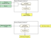 |
Fig. B.1. Signal and noise ring-set creation pipelines. |
In the same manner, we create ring-sets for each of the specific systematic effects we would like to measure. We add together signal, noise, and systematic ring-sets, and, given models for straylight (based on the GRASP beams) and the orbital dipole, we create “perfectly-calibrated” ring-sets (calibration constant = 1). We use the gains estimate from the 2018 data release to “de-calibrate” these timelines, in other words, to convert them from kelvins to volts. At this point the calibration pipeline starts, and produces the reconstructed gains that will be different from the ones used in the de-calibration process due to the presence of simulated systematic effects. The calibration pipeline is algorithmically exactly the same as that used at the DPC for product creation, but with a different implementation (based principally on python). The gain-smoothing algorithm is the same as used for the data, and has been tuned to the actual data. This means that there will be cases where reconstructed gains from simulations differ significantly from the input ones. We have verified that this indeed happens, but only for very few pointing periods, and we therefore decided not to consider them in the following analysis. The overall process for estimating gains is given in Fig. B.2.
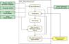 |
Fig. B.2. Gain reconstruction pipeline. |
At this point we are able to generate maps for full mission, half-ring, and odd-even-year splits) that include the effects of systematic errors on calibration. In the final step, we produce timelines (which are never stored) starting from the same fiducial sky map, using the same model for straylight and the orbital dipole as in the previous steps, and from generated noise-only timelines created with the same seeds and noise model used before. We then apply the official gains to “de-calibrate” the timelines, which are immediately calibrated with the reconstructed gains in the previous step. The nominal destriping mapmaking algorithm is then used to create final maps. The complete data flow is given in Fig. B.3.
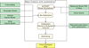 |
Fig. B.3. Final simulation step, where calibrated maps are created from reconstructed gains, including the impact of systematic effects. |
All Tables
Percentage of LFI observation time lost due to missing or unusable data, and to manoeuvres.
Additional noise in μK2 from systematic effects for three different multipole ranges (ℓ = 4–5, ℓ ≃ 100, and ℓ ≃ 500).
All Figures
|
Fig. 1. Schematic representation of the LFI data-processing pipeline from raw telemetry down to frequency maps. Elements in red are those changed or improved with respect to Planck Collaboration II (2016). |
| In the text | |
|
Fig. 2. Normalized gain difference (see main text for precise definition) between two radiometers inside the same horn (28M and 28S here) as a function of pointing ID for both the 2015 (DX11D) and 2018 calibration schemes. The coloured lines show this function for the various iterations in the new {gain-estimation + mapmaking + component separation} calibration scheme. Sky surveys are indicated by alternating white and grey vertical bands. Other 30- and 44 GHz radiometers show qualitatively similar behaviour, whereas the 70 GHz radiometers exhibit too much noise, and corresponding iterations for these detectors do not converge within this scheme. |
| In the text | |
|
Fig. 3. Same as Fig. 2, but stacked over surveys. Each band corresponds to the mean and 1σ confidence region as evaluated from eight surveys. |
| In the text | |
|
Fig. 4. Polarization amplitude difference maps between consecutive iterations of the internal foreground model evaluated at 30 GHz, as derived with Commander. The three panels show the differences between: the second and first iterations (top); the third and second iterations (middle); and the fourth and third iterations (bottom). All maps are smoothed to an effective angular resolution of 8° FWHM. |
| In the text | |
|
Fig. 5. Final low-resolution LFI 2017 polarization amplitude sky maps. From top to bottom, the panels show the co-added 30-, 44-, and 70 GHz frequency maps. The grey regions indicate the mask used during gain calibration. Each pixel is 3 |
| In the text | |
|
Fig. 6. Gain correction template for the 70 GHz channel in terms of Stokes Q (top) and U (middle), and the polarization amplitude, P (bottom). The template is smoothed to 2° FWHM, and its amplitude is normalized to the best-fit value derived in a joint maximum likelihood analysis of both the CMB power spectrum and template fit, as described in the text. |
| In the text | |
|
Fig. 7. 30 GHz polarization amplitude null maps evaluated between survey combinations {S1,S3, S5–8} and {S2, S4} for both the 2015 (top) and 2018 (bottom) calibration schemes. This particular survey split is maximally sensitive to residual gain uncertainties from polarized Galactic foreground contamination because of the orientation of the scanning strategy employed in Surveys 2 and 4; see text and Planck Collaboration II (2016) for further details. Both maps are smoothed to an effective angular resolution of 8° FWHM. |
| In the text | |
|
Fig. 8. Direction (top) and amplitude (bottom) of the solar dipole determined from each of the LFI detectors. Uncertainties in direction are given by 95% ellipses around symbols, colour-coded for frequency (70 GHz black or unfilled, 44 GHz green, and 30 GHz red). The four discrepant points are at 30 GHz, where we expect foregrounds affect dipole estimation. Amplitude uncertainties are dominated by the systematic effects of gain uncertainties. The grey band in the bottom panel shows the WMAP dipole amplitude for comparison. |
| In the text | |
|
Fig. 9. Evolution of noise spectra over the mission lifetime for radiometer 18M (70 GHz, top), 25S (44 GHz, middle), and 27M (30 GHz, bottom). Spectra are colour-coded, ranging from OD 100 (blue) to OD 1526 (red), with intervals of about 20 ODs. White-noise levels and slope stability are considerably better than in the 2015 release, being at the 0.1% level for noise, while knee-frequencies show variations at the 1.5% level. |
| In the text | |
|
Fig. 10. LFI maps at 30 GHz: top: total intensity I; middle: Q polarization component; bottom: U polarization component. Stokes I is shown at instrument resolution and at Nside = 1024, while Q and U are smoothed to 1° resolution and at Nside = 256. Units are μKCMB. The polarization components have been corrected for bandpass leakage (Sect. 7). |
| In the text | |
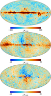 |
Fig. 11. Same as Fig. 10, for the 44 GHz channel. |
| In the text | |
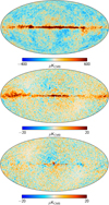 |
Fig. 12. Same as Fig. 10, for the 70 GHz channel. |
| In the text | |
|
Fig. 13. Differences between 2018 (PR3) and 2015 (PR2) frequency maps in I, Q, and U. Maps are smoothed to 1° angular resolution for I and to 3° for Q and U, in order to highlight large-scale features. Differences are clearly evident at 30 and 44 GHz, and are mainly due to changes in the calibration procedure. |
| In the text | |
|
Fig. 14. Differences between odd (i.e., Surveys 1, 3, 5, and 7) and even (Surveys 2, 4, 6, and 8) surveys in I, Q, and U (from left to right) for the 2015 (upper nine maps) and 2018 (lower nine maps) data releases. These maps are smoothed to 3 deg to reveal large-scale structures. |
| In the text | |
|
Fig. 15. Angular pseudo-power spectra of the odd-even survey difference maps for 30 (left column), 44 (middle column), and 70 GHz (right column), with the 2015 data in purple and 2018 in green. |
| In the text | |
|
Fig. 16. Survey difference maps of polarization amplitude at 30 GHz for the current 2018 (right) and 2015 (left) releases. The improvement is evident, especially in odd-even difference maps, showing lower residuals due to the new calibration approach. Maps are smoothed with an 8 deg Gaussian beam to show large-scale structures. |
| In the text | |
|
Fig. 17. Null-test results comparing power spectra from survey differences to those from the half-ring maps. Differences are: left: Survey 1 − Survey 2; middle: Survey 1 − Survey 3; and right: Survey 1 − Survey 4. These are for 30 GHz (top), 44 GHz (middle), and 70 GHz (bottom), for both TT and EE power spectra. There is a significant improvement in Survey 1 − Survey 2 and Survey 1 − Survey 4 at 30 GHz, especially in EE. |
| In the text | |
|
Fig. 18. Consistency check at the power spectrum level between half-ring difference maps (red), white-noise covariance matrices (black dash-dotted lines), and 100 full-noise MC simulations (grey band showing range for 16% and 84% quantiles of noise simulations, and the black solid lines giving the median, i.e., 50% quantile, of the distributions). From top to bottom we show TT, EE, and BB power spectra for 30 GHz (left), 44 GHz (centre), and 70 GHz (right). Half-ring spectra are binned with Δℓ = 25 for ℓ ≥ 75. |
| In the text | |
|
Fig. 19. Ratio of mean noise at high multipoles (1150 ≤ ℓ ≤ 1800) to white noise, derived from white-noise covariance matrices produced during the mapmaking process. |
| In the text | |
|
Fig. 20. Binned TT cross-spectra from half-ring maps at 30, 44, and 70 GHz. Foregrounds are accounted for only through the use of the proper frequency-dependent Galactic masks. Red-dashed lines are the Planck best-fit TT spectrum, to which a contribution from unresolved point sources (specific to each frequency) has been added. |
| In the text | |
|
Fig. 21. Scatter plots of LFI angular cross-spectra around the first acoustic peak for frequency pairs: left: 70 GHz and 30 GHz; middle: 70 GHz and 44 GHz; right: 44 GHz and 30 GHz. The solid line is the linear fit obtained accounting for error bars on both axes. Slopes, within expected uncertainty, show good consistency among data sets |
| In the text | |
|
Fig. 22. Residuals between cross-spectra at 70 GHz from half-ring (HR) and year maps (YR). Error bars come from FFP10 Monte Carlo simulations. |
| In the text | |
|
Fig. 23. Empirical distributions derived from FFP10 simulations for the s1, s2, and s3 statistics of the Hausman test on the 70 GHz data. Vertical lines show values derived from half-ring and year maps at 70 GHz. |
| In the text | |
|
Fig. 24. Odd-even-year null spectra compared with simulations including the gain smoothing algorithm at 30 (left), 44 (middle), and 70 GHz (right). The pink band shows the 16%–84% quantile range of the simulations, with the median traced by the blue line. On large angular scales the data show larger variations with multipole than the simulations. |
| In the text | |
|
Fig. 25. Angular TT (top) and EE (bottom) power spectra at 30 (left), 44 (middle), and 70 GHz (right) of a complete set of systematic effects for the 2015 data release (red) and the 2018 simulations (blue, 50% percentile plus 1σ band from simulations). This shows the good agreement between the two releases. In green we show the null spectra from odd-even year difference. The CMB angular power spectra (black lines) are convolved with the frequency dependent window functions. |
| In the text | |
|
Fig. A.1. Stokes Q difference maps between Planck 30 GHz 2015 (top) and 2018 (bottom) and WMAP K-band (left) and Ka-band (right). The WMAP K and Ka band maps are rescaled to match the Planck 30 GHz effective frequency assuming synchrotron emission with a spectral index of −3. All maps used in this comparison have been smoothed with a 10 deg Gaussian beam. |
| In the text | |
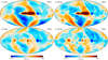 |
Fig. A.2. Same as in Fig. A.1, for Stokes U. |
| In the text | |
|
Fig. B.1. Signal and noise ring-set creation pipelines. |
| In the text | |
|
Fig. B.2. Gain reconstruction pipeline. |
| In the text | |
|
Fig. B.3. Final simulation step, where calibrated maps are created from reconstructed gains, including the impact of systematic effects. |
| In the text | |
Current usage metrics show cumulative count of Article Views (full-text article views including HTML views, PDF and ePub downloads, according to the available data) and Abstracts Views on Vision4Press platform.
Data correspond to usage on the plateform after 2015. The current usage metrics is available 48-96 hours after online publication and is updated daily on week days.
Initial download of the metrics may take a while.