| Issue |
A&A
Volume 632, December 2019
|
|
|---|---|---|
| Article Number | A46 | |
| Number of page(s) | 26 | |
| Section | Stellar structure and evolution | |
| DOI | https://doi.org/10.1051/0004-6361/201935745 | |
| Published online | 26 November 2019 | |
X-shooter spectroscopy of young stars with disks
The TW Hydrae association as a probe of the final stages of disk accretion⋆⋆⋆
1
Eberhard Karls Universität, Institut für Astronomie und Astrophysik, Sand 1, 72076 Tübingen, Germany
2
Department of Astronomy, Cornell University, Space Sciences Building, Ithaca, NY 14853, USA
3
NASA Ames Research Center, Moffett Blvd, Mountain View, CA 94035, USA
e-mail: This email address is being protected from spambots. You need JavaScript enabled to view it.
4
INAF – Osservatorio Astronomico di Palermo, Piazza del Parlamento 1, 90134 Palermo, Italy
5
INAF – Osservatorio Astronomico di Capodimonte, Salita Moiariello 16, 80131 Napoli, Italy
6
European Southern Observatory, Karl-Schwarzschild-Strasse 2, 85748 Garching bei München, Germany
7
INAF – Osservatorio Astrofisico di Catania, via S. Sofia, 78, 95123 Catania, Italy
8
INAF – Osservatorio Astronomico di Roma, via di Frascati 33, 00078 Monte Porzio Catone, Italy
9
Dipartimento di Fisica e Chimica, Università degli Studi di Palermo, Piazza del Parlamento 1, 90134 Palermo, Italy
10
Dublin Institute for Advanced Studies, 31 Fitzwilliam Place, Dublin 2, Ireland
11
INAF – Osservatorio Astrofisico di Arcetri, Largo E. Fermi 5, 50125 Florence, Italy
12
SUPA, School of Physics & Astronomy, University of St Andrews, North Haugh, St Andrews KY169SS, UK
Received:
21
April
2019
Accepted:
6
September
2019
Abstract
Context. Measurements of the fraction of disk-bearing stars in clusters as a function of age indicate protoplanetary disk lifetimes ≲10 Myr. However, our knowledge of the time evolution of mass accretion in young stars over the disk lifespans is subject to many uncertainties, especially at the lowest stellar masses (M⋆).
Aims. We investigate ongoing accretion activity in young stars in the TW Hydrae association (TWA). The age of the association (∼8–10 Myr) renders it an ideal target for probing the final stages of disk accretion, and its proximity (∼50 pc) enables a detailed assessment of stellar and accretion properties down to brown dwarf masses.
Methods. Our sample comprises eleven TWA members with infrared excess, amounting to 85% of the total TWA population with disks. Our targets span spectral types between M0 and M9, and masses between 0.58 M⊙ and 0.02 M⊙. We employed homogeneous spectroscopic data from 300 nm to 2500 nm, obtained synoptically with the X-shooter spectrograph, to derive the individual extinction, stellar parameters, and accretion parameters for each object simultaneously. We then examined the luminosity of Balmer lines and forbidden emission lines to probe the physics of the star–disk interaction environment.
Results. Disk-bearing stars represent around 24% of the total TWA population. We detected signatures of ongoing accretion for 70% of our TWA targets for which accurate measurements of the stellar parameters could be derived. This implies a fraction of accretors between 13–17% across the entire TWA (that accounts for the disk-bearing and potentially accreting members not included in our survey). The spectral emission associated with these stars reveals a more evolved stage of these accretors compared to younger PMS populations studied with the same instrument and analysis techniques (e.g., Lupus): first, a large fraction (∼50%) exhibit nearly symmetric, narrow Hα line profiles; second, over 80% of them exhibit Balmer decrements that are consistent with moderate accretion activity and optically thin emission; third, less than a third exhibit forbidden line emission in [O I] 6300 Å, which is indicative of winds and outflows activity; and fourth, only one sixth exhibit signatures of collimated jets. However, the distribution in accretion rates (Ṁacc) derived for the TWA sample closely follows that of younger regions (Lupus, Chamaeleon I, σ Orionis) over the mass range of overlap (M⋆ ∼ 0.1–0.3 M⊙). An overall correlation between Ṁacc and M⋆ is detected and best reproduced by the function Ṁacc ∝ M∝2.1±0.5.
Conclusion. At least in the lowest M⋆ regimes, stars that still retain a disk at ages ∼8–10 Myr are found to exhibit statistically similar, albeit moderate, accretion levels as those measured around younger objects. This “slow” Ṁacc evolution that is apparent at the lowest masses may be associated with longer evolutionary timescales of disks around low-mass stars, which is suggested by the mass-dependent disk fractions reported in the literature within individual clusters.
Key words: accretion / accretion disks / techniques: spectroscopic / stars: low-mass / stars: pre-main sequence / open clusters and associations: individual: TWA
Reduced spectra are also available at the CDS via anonymous ftp to cdsarc.u-strasbg.fr (130.79.128.5) or via http://cdsarc.u-strasbg.fr/viz-bin/cat/J/A+A/632/A46
Based on observations collected at the European Southern Observatory under ESO programs 084.C–0269(B), 085.C–0238(A), 086.C–0173(A), 087.C–0244(A), 287.C–5039(A), 089.C–0143(A), 093.C–0097(A), and 095.C–0147(A).
NASA Postdoctoral Program (NPP) fellow.
© ESO 2019
1. Introduction
Disks are a ubiquitous result of the earliest stages of star formation, and surround the majority of low-mass stars at an age of ∼1 Myr. Over the next few million years, the interaction between the inner disk and the central object is regulated by the process of magnetospheric accretion (see Hartmann et al. 2016 for a recent review). This process has a profound impact on the inner disk evolution and on the fundamental properties of the nascent star, such as mass and angular momentum. It also has a direct impact on planet formation, as it alters the respective gas and dust contents of the disk, modifies the local disk structure, and can trigger or halt planet migration within the disk (Alexander et al. 2014; Morbidelli & Raymond 2016).
Observational studies of disk frequencies in young star clusters as a function of age (e.g., Hernández et al. 2007; Fedele et al. 2010; Ribas et al. 2014) indicate that disks are typically cleared within a timescale of ∼10 Myr. However, the evolution of disk accretion during this time frame is not constrained as well. Indeed, while it has been shown that the characteristic timescale of disk accretion (as inferred from counting the fraction of accreting stars in populations of different ages; Jayawardhana et al. 2006; Fedele et al. 2010) is slightly shorter than that of dust dissipation in the inner disk, the actual age dependence of disk accretion remains to be elucidated.
Extensive compilations of mass accretion rates (Ṁacc) in pre-main sequence (PMS) stellar populations have been published in recent years, making use of several accretion tracers: the continuum excess emission which arises from the accretion shock at the stellar surface (e.g., Herczeg & Hillenbrand 2008; Ingleby et al. 2013; Alcalá et al. 2014, 2017; Manara et al. 2017a); the U-band flux excess used as a probe of the total accretion luminosity, Lacc (e.g., Rigliaco et al. 2011; Manara et al. 2012; Venuti et al. 2014); the Hα line emission (e.g., De Marchi et al. 2010; Kalari et al. 2015; Sousa et al. 2016; Biazzo et al. 2019) or other emission lines (e.g., Mohanty et al. 2005; Nguyen et al. 2009; Antoniucci et al. 2011, 2014; Caratti o Garatti et al. 2012) that arise from the heated gas in the accretion columns. Such surveys have enabled, for instance, detailed assessments of the relationship between Ṁacc and the stellar mass (M⋆), a key observational constraint when validating theories on the dynamics of accretion and of disk evolution (Alexander & Armitage 2006; Dullemond et al. 2006; Hartmann et al. 2006; Vorobyov & Basu 2008; Ercolano et al. 2014). However, many of the well-studied PMS populations only sample the first few (≲3–5) Myr of the early stellar evolution (see the works of Ingleby et al. 2014 and Rugel et al. 2018 on accretion in older PMS stars). Tentative relationships between Ṁacc and age have been extrapolated from intra-cluster accretion surveys, by combining Ṁacc measurements and age estimates of individual cluster members (e.g., Sicilia-Aguilar et al. 2010; De Marchi et al. 2010; Manara et al. 2012; Antoniucci et al. 2014; Hartmann et al. 2016). Such studies suggest an age dependence of Ṁacc(t) ∝ t−(1.3 ± 0.3); however, this approach is subject to the strong uncertainty on individual age estimates for young stars (Soderblom et al. 2014), and to the interplay between age-related effects and mass-related effects in Ṁacc.
Given its proximity and age, the TW Hydrae association (TWA) is an ideal target to probe disk accretion during its final stages when gas-rich disks evolve into debris disks. Located at a distance of about 50 pc (Weinberger et al. 2013), it is the closest stellar association containing PMS stars with active accretion disks. The most recent census of the TWA (Gagné et al. 2017) encompasses 55 bona fide members or high-likelihood candidate members, with or without disks, which are distributed in a total of 34 star systems (some comprising multiple stars). The bulk of these sources have spectral type (SpT) between late-K and either late-M or early-L. Recent age estimates for the TWA oscillate between ∼8 Myr (e.g., Ducourant et al. 2014; Herczeg & Hillenbrand 2014; Donaldson et al. 2016) and ∼10 Myr (Bell et al. 2015), and the association exhibits a disk fraction of nearly 25% in the M-type spectral class (Schneider et al. 2012; Fang et al. 2013a). Signatures of ongoing disk accretion in TWA members have been reported by Muzerolle et al. (2001), Scholz et al. (2005), Jayawardhana et al. (2006), Stelzer et al. (2007), Herczeg et al. (2009), and Looper et al. (2010), for example. The proximity of the association renders each of its members, down to masses ≲0.05 M⊙, accessible for detailed individual characterization. In spite of a limited population number, the TWA therefore provides key observational constraints in undersampled areas of the multi-parameter space (e.g., stellar mass, disk mass, accretion rate, stellar multiplicity) that governs the evolution of young stars and their disks.
We have recently conducted an extensive spectroscopic survey of TWA members with signatures of disks, making use of the wide-band spectrograph X-shooter (Vernet et al. 2011) at the ESO Very Large Telescope (VLT). Thanks to its broad synoptic wavelength coverage, which extends from ∼300 nm to 2500 nm, X-shooter is especially suited to investigate accretion in young stars: it provides access to a rich variety of accretion diagnostics (excess continuum, Balmer series, multiple optical and near-infrared emission lines), and enables measuring the extinction, photospheric flux, stellar parameters, and accretion parameters simultaneously, with no ambiguity related to the intrinsic variability of young stars (e.g., Costigan et al. 2014; Venuti et al. 2015). Systematic surveys of accretion in various star-forming regions have been conducted with X-shooter in the past few years (see Rigliaco et al. 2012 in the ∼6 Myr-old σ Orionis; Manara et al. 2015 in the 1–3 Myr-old ρ Ophiucus; Alcalá et al. 2017 in the < 3 Myr-old Lupus; Manara et al. 2017a in the 2–3 Myr-old Chamaeleon I; Rugel et al. 2018 in the ∼11 Myr-old η Chamaeleontis). The extent and homogeneity of such surveys has enabled, for instance, assessing the presence of a bimodality in the Ṁacc − M⋆ distribution at masses < 2 M⊙ and ages ≤3 Myr, with a steeper Ṁacc − M⋆ relationship in the lower-mass regime than in the higher-mass regime, and a break in the relationship at M⋆ ∼ 0.2 − 0.3 M⊙ (Alcalá et al. 2017; Manara et al. 2017a). In addition, a synergy between X-shooter and ALMA (Ansdell et al. 2016) surveys provided first observational evidence of a correlation between Ṁacc and disk dust masses Mdisk, dust in the Lupus cloud (Manara et al. 2016) and in the Chamaeleon I region (Mulders et al. 2017).
To complement the efforts mentioned above and extend them toward the final stages of disk accretion, we present here the X-shooter view of the accretion process across the TWA. The analysis was conducted with the same approach and methods pursued in previous X-shooter surveys of accretion in younger star-forming regions. This enables a direct and internally consistent comparison of our results to the accretion properties of the ρ Oph, Lupus, Cha I, σ Ori, and η Cha populations, aimed to constrain the evolution of disk accretion across the pre-main sequence phase, from subsolar to brown dwarf stellar masses.
Our paper is organized as follows. Section 2 provides a description of the observations used in this work, and of their reduction. In Sect. 3.1 we describe the procedure adopted to derive the stellar and accretion parameters for our targets. The resulting picture of accretion across the TWA is presented in Sect. 3.2, and information on the accretion dynamics and on the accretion and ejection processes for individual TWA members is presented in Sect. 3.3. Our results are discussed in Sect. 4, in the context of the evolution of disk accretion and of the impact of stellar parameters, disk parameters, and environmental conditions. Our conclusions are summarized in Sect. 5.
2. Sample, observations, and data reduction
2.1. Target selection
Our sample comprises 14 stars, selected among the confirmed or putative TWA members upon showing evidence of circumstellar material from mid-infrared excess in Spitzer/IRAC (Fazio et al. 2004) or WISE (Wright et al. 2010) bands. A complete list of the targets is reported in Table 1; several sources are part of multiple systems. Our targets include TWA 3B, a companion of the spectroscopic binary TWA 3A. This star is reported to be non-accreting from earlier Balmer continuum or Hα emission measurements (e.g., Herczeg et al. 2009). Furthermore, no evidence of infrared excess up to wavelengths of ∼10 μm has been detected in earlier surveys (Jayawardhana et al. 1999a,b), which indicates that the disk around this star (if present) is devoid of material in the inner regions. For these reasons, we excluded TWA 3B from any statistical analysis regarding the accretion activity in the TWA, but we report and discuss all parameters derived from our data on this target in Appendix A.
Log of X-shooter observations.
To our knowledge, and based on the latest census of the TWA (Gagné et al. 2017), our survey of accreting sources in the association is ∼85% complete in regard to its disk-hosting population. Two of the targets in our list (TWA 22 and TWA 31) were recently disputed as TWA members, and proposed to be members of the β Pictoris moving group and of the Lower Centaurus Crux association, respectively (Gagné et al. 2017). This would place them at slightly older ages than the TWA, 24 Myr (Bell et al. 2015) and 17–23 Myr (Mamajek et al. 2002), respectively. We used the newest astrometric data from Gaia DR2, together with radial velocity measurements for our targets, to derive their space velocities with respect to nearby young stellar associations. This analysis indicates that, while TWA 22 appears a more likely member of the β Pictoris association than of the TWA, TWA 31 falls among the confirmed TWA members on u, v, w diagrams. For consistency with the lower membership probability calculated by Gagné et al. (2017) for these two objects, in the following we keep them separate from the other targets when discussing the statistical inferences from our survey. Therefore, after excluding TWA 3B, the final sample of TWA members that are the focus of our study amounts to eleven stars with infrared excess. We note that our results would not change appreciably if all objects were included at every step of the analysis.
2.2. Observations and data processing
The observations were conducted in the course of multiple programs between 2010 and 2015, as reported in Table 1. Programs 084.C-0269, 085.C-0238, 086.C-0173, 087.C-0244, and 089.C-0143 (PI Alcalá) were performed as part of the X-shooter guaranteed-time observations (GTO; Alcalá et al. 2011) granted to the Italian Istituto Nazionale di AstroFisica (INAF) as member of the X-shooter consortium. Programs 093.C-0097 and 095.C-0147 (PI Stelzer) were performed later to expand the GTO survey of the TWA. More than one spectrum were acquired for some objects in the target list (TWA 1, TWA 27, TWA 30), either on the same date but using different exposure time (TWA 1) or slit width (TWA 30), or on different epochs (TWA 27) to constrain their time variability. TWA 30A and TWA 30B were additionally observed with X-shooter in the Director’s Discretionary Time (DDT) program 287.C-5039 (PI Sacco).
X-shooter comprises three spectroscopic arms, operating simultaneously in three different spectral windows: UVB (300–555 nm), VIS (545–1035 nm), and NIR (995–2480 nm). For the brightest sources in our sample, observations were acquired using slit widths of 0.5″/0.4″/0.4″ in the UVB/VIS/NIR arms, respectively, yielding a resolution R ∼ 9700/18400/11600. Fainter sources were instead observed using slit widths of 1.0″/0.9″/0.9″ (corresponding to R ∼ 5400/8900/5600) or 1.6″/1.5″/1.2″ (corresponding to R ∼ 3200/5000/4300), respectively, in the UVB/VIS/NIR arms. Observations were conducted in nodding mode, either using a one-cycle A–B pattern (two exposures), or a two-cycle A–B–B–A pattern (four exposures). For the faintest source in the target list (TWA 40), two cycles of observations with the A–B–B–A nodding mode were performed, and the resulting frames were combined to increase the signal-to-noise ratio (S/N).
The spectra were reduced using the latest version of the X-shooter pipeline (Modigliani et al. 2010) available at the end of each observing program: versions 1.0.0, 1.3.0, and 1.3.7 were used for the data from periods P084 through P089, and version 2.8.4 was employed for periods P093 and P095. The data reduction steps include bias (UVB, VIS) or dark current (NIR) subtraction, flat-field correction, wavelength calibration, measurement of the instrument resolving power, determination of the instrument response and global efficiency, sky subtraction, and flux calibration. The final one-dimensional spectra were then extracted from the pipeline output two-dimensional spectra by using the specred package in the Image Reduction and Analysis Facility (IRAF1) software (Tody 1986). This step was performed with the IRAF task apall, which involves visual optimization of the aperture for flux extraction around the bright signature of the source in the two-dimensional spectrum, and correction for deviations of the source signature from a straight baseline across the spectrum.
2.3. Telluric correction and flux calibration
The extracted one-dimensional spectra were subsequently corrected for telluric features in their VIS and NIR segments. For the observing programs in cycles P089 and earlier, the telluric correction was carried out as described in Appendix A of Alcalá et al. (2014). Namely, the spectra of the target stars were divided by the spectra of telluric standard stars, observed very close in time to the science target at a similar airmass, after normalizing the telluric spectra to their continuum and removing any stellar lines from the normalized spectra. A scaling factor was introduced in the procedure to account for small differences in airmass between the observing epochs of target star and telluric standard. For spectra acquired during the more recent observing programs, the telluric correction was handled with the molecfit tool (Smette et al. 2015; Kausch et al. 2015). A transmission spectrum of the Earth’s atmosphere, accounting for the altitude of the observing site and for the local conditions of temperature, pressure, and humidity at the time of the observation, is computed by fitting an atmospheric radiative transfer model to selected telluric regions of the science spectrum, and then using the best-fit parameters (spectral line profile, molecular column densities) to calculate the transmission spectrum over the entire wavelength range. The telluric-corrected spectrum is then obtained by dividing the science spectrum by the generated transmission curve. To verify the consistency between the two methods of telluric correction, we ran molecfit on several spectra of young stars acquired by our group in different regions, and originally corrected following the method in Alcalá et al. (2014). We then compared the telluric-corrected spectra obtained for a given source with the two methods, and could ascertain that the two corrections overlap correctly within the intrinsic spectrum noise.
To account for potential flux losses within the slit, we recalibrated the spectra to the tabulated J-band photometry for the objects from the 2MASS survey (Skrutskie et al. 2006). We converted the observed magnitudes to fluxes, using the zero-point flux provided by the SVO Filter Profile Service (Rodrigo et al. 2012), and multiplied the NIR part of the spectrum by the ratio between the J-band flux and the average spectrum flux over the J-bandpass. We then used the overlapping wavelength regions between the NIR and VIS and between the VIS and UVB parts of the spectra to align them in flux. The match was performed by computing the point-by-point flux ratio between two neighboring spectrum segments across the overlapping region, and then taking as corrective factor the median of the measured point-by-point flux ratios, after ascertaining that the VIS/NIR and UVB/VIS flux ratios calculated point by point are not dependent on wavelength.
In Fig. 1, one example of the reduced and telluric-corrected spectra from our sample is shown for illustration purposes.
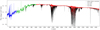 |
Fig. 1. Final processed X-shooter spectrum of TWA 32, separated into UVB (blue), VIS (green), and NIR (red) segments, after correction for telluric features with molecfit and removal of most prominent spikes. The source spectrum after the pipeline reduction but before the telluric correction is shown in black for comparison. |
3. Results
3.1. Stellar and accretion parameters
In the following we describe the procedure adopted to determine individual extinctions, spectral types, stellar luminosities, and accretion luminosities (Sect. 3.1.1), atmospheric parameters, radial velocities, projected rotational velocities, and veiling (Sect. 3.1.2), and stellar masses, radii, and mass accretion rates (Sect. 3.1.3) across our sample.
3.1.1. SpT, AV, L⋆, and Lacc
To estimate the SpT, extinction (AV), stellar luminosity (L⋆), and Lacc of all but the faintest sources in our sample (J1247−3816 and TWA 40; see below), we adopted the same method introduced in Manara et al. (2013a). In brief, a multi-component fit to the observed spectrum was carried out. The fit includes: a set of photospheric templates, consisting of X-shooter spectra of well-characterized, non-accreting young stars, to reproduce the photospheric and chromospheric emission of PMS stars with SpT between late-K and late-M (Manara et al. 2013b, 2017b); a standard interstellar reddening law with RV = 3.1 (Cardelli et al. 1989), and a grid of AV values from 0 to several magnitudes of extinction; and finally an isothermal hydrogen slab2 model, with varying temperature, electron density, and optical depth, to reproduce the emission from the accretion shock. For each point of the model grid explored (i.e., a different combination of photospheric template spectrum, AV value, slab parameters described above, and two normalization factors for the photospheric and slab emission), the model spectrum is compared to the observed spectrum in several spectral features: flux ratio at the Balmer jump (i.e., between ∼360 and 400 nm), slope of the Balmer continuum (332.5–360 nm), slope of Paschen continuum (398–477 nm), and the continuum flux level in selected, narrow (∼2 nm–wide) wavelength intervals across the spectrum (at ∼360 nm, ∼460 nm, ∼703 nm, ∼707 nm, ∼710 nm, and ∼715 nm). A χ2-like function3 is computed to measure the degree of agreement between each model fit and the observed spectrum. The best-fit parameters are determined by minimizing the χ2-like distribution. Parameters derived simultaneously via this procedure are not impacted by the degeneracy between circumstellar extinction and accretion, which affect the continuum spectrum from the UV to the NIR in a very different way: extinction reduces the observed stellar luminosity and is more efficient at shorter wavelengths, therefore making the source appear redder, hence colder, than it actually is; accretion produces a luminosity excess that peaks in the UV, which makes the source appear bluer, hence hotter and brighter, than it actually is.
The L⋆ and Lacc values were scaled using the individual distances to TWA members computed from Gaia DR2 (Gaia Collaboration et al. 2018) parallaxes. These distances are in most cases consistent with the distances listed for each object in Gagné et al. (2017), within the combined uncertainty from the new Gaia parallax errors and from the errors on the previous distance estimates. For two sources, the absolute difference between new and old distance values is more than three times larger than the total uncertainty: these are TWA 27 (previous distance 52.8 ± 1.0 pc, new distance 64.4 ± 0.7 pc) and TWA 22 (previous distance 17.5 ± 0.2 pc, new distance 19.61 ± 0.12 pc). Another two sources (J1247−3816 and TWA 28) exhibit a change in estimated distance about twice as large as the combined uncertainty. The change in distance is more marked for J1247−3816 (previous distance 68 pc, new distance 85 pc); however, this is also the source with the largest uncertainty on the distance estimate among our sample. The values of individual distances adopted here and the derived parameters for each star are reported in Table 2.
Results of the procedure described above are illustrated in Fig. F.1. The star TWA 30B appears as a severely underluminous object due to its edge-on configuration (Looper et al. 2010); we therefore exclude this star from Fig. F.1 and from subsequent analyses involving the estimated L⋆. For the remaining targets (except J1247−3816 and TWA 40, as discussed in the next paragraph), we evaluated the significance of the Lacc detection by comparing the luminosity of the observed spectrum to the normalized spectrum of the photospheric template in the Balmer continuum region (λ ∼ 332.5–360 nm). Namely, we sampled this spectral window in 2.5 nm–wide intervals, and for each interval we compared the median flux of the science target to the median flux of the photospheric template. The large noise that affects this region of the spectra, particularly for the photospheric templates, hampers a strict definition of a quantitative threshold to separate “accretion–dominated” from “chromospheric–dominated” objects. We therefore decided to sort our objects into three groups: bona fide accretors (5 objects), when the median flux measured for the science target across the Balmer continuum is systematically higher than that measured for the photospheric template, and the difference between the two is larger than the total rms spectral noise; possible accretors (4), when the science targets exhibit systematically higher median flux than the photospheric templates across the Balmer continuum, but with a flux difference comparable to the total rms noise; and upper limits (1), when the median flux measured for the science object is higher than that measured for the photospheric template only in some portions of the Balmer continuum. Separate lists for the objects that fall into each group are reported in Table 2.
For the two faintest sources of our sample (J1247−3816 and TWA 40), no solution could be determined with the multi-component fit, due to poor S/N in the UVB part of the spectrum. We therefore followed the approach of Manara et al. (2015, also used for consistency checks in Stelzer et al. 2013 and Alcalá et al. 2014, 2017) to estimate the SpT and AV of these two objects. We used photospheric templates of varying SpT from the grid of X-shooter spectra of young non-accreting stars from Manara et al. (2013b, 2017b); these were artificially reddened following the reddening law of Cardelli et al. (1989) for RV = 3.1, with AV allowed to vary between 0 and 3 mag. At each step in AV, we then normalized the spectrum of the reddened template to the observed spectrum around λ ∼ 1025 nm, and computed a χ2-like function which samples the discrepancy between the observed spectrum and the reddened template in 24 spectral windows, each a few nm wide, distributed between λ = 700 nm and λ = 1700 nm. The best (SpT, AV) solution was then determined via χ2-like minimization.
Independent estimates of SpT were derived for the whole sample by computing a variety of spectral indices (Allers et al. 2007; Jeffries et al. 2007; Riddick et al. 2007; Scholz et al. 2012; Rojas-Ayala et al. 2012; Herczeg & Hillenbrand 2014), which probe the depth of Teff–dependent molecular bands in the VIS and NIR spectra. The best SpT was computed as the average of the individual SpT estimates from the various spectral indices, after excluding those estimates that would fall outside the range of validity specified in the literature for the corresponding spectral index. An a posteriori consistency check between the SpT estimates from our multi-component fit and those from the spectral indices analysis allowed us to identify which sets of spectral indices work best in a given SpT range. In turn, this analysis allowed us to better constrain the (SpT, AV) solution for J1247−3816 and TWA 40 from the spectral fit. The L⋆ of these two stars was then estimated from the luminosity of the template corresponding to the (SpT, AV) solution, with a scaling factor that accounts for the flux and squared distance ratio between the target and the template.
In Fig. 2 we compare our measurements of L⋆ with results from previous surveys and compilations for objects in common (Ducourant et al. 2014; Kastner et al. 2016), rescaled to the values of distances adopted in this study. The diagram shows an overall agreement between different sets of measurements for the bulk of sources, with most L⋆ estimates lying close to the identity line on Fig. 2.
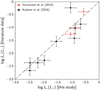 |
Fig. 2. Comparison between our L⋆ estimates (see Sect. 3.1.1 and Table 2) and values reported by Ducourant et al. (2014, red symbols) and Kastner et al. (2016, black symbols), corrected for difference in distance between our adopted values and values listed in those references for individual objects. The error bars trace the individual uncertainties associated with the L⋆ values in the compilation of Ducourant et al. (2014), and a typical uncertainty of ±0.2 dex in the other cases, for illustration purposes. The identity line is dashed in gray to guide the eye. |
3.1.2. Teff, log g, radial velocity, v sin i, veiling
To determine the atmospheric parameters (Teff, log g) of the stars and their radial velocities (RV), projected rotational velocities (v sin i), and veiling (r), we made use of the ROTFIT code (Frasca et al. 2017). In brief, BT-Settl synthetic spectra (Allard et al. 2012), degraded to match the instrument resolution, were used as templates to fit the observed spectra around spectral features particularly sensitive to the parameters of interest. Both observed spectra and templates were normalized to the local continuum before the fitting procedure, which was implemented via a χ2 routine. The fitting regions were chosen primarily in the VIS window, and selected so as to avoid any contamination from accretion or chromospheric signatures. The rotational broadening effects were simulated in the synthetic templates by convolving them with a rotational profile across a grid of v sin i values. The effects of veiling were described as (Fλ/FC)r = (Fλ/FC+r)/(1+r), where Fλ represents the line flux, FC the continuum flux, and r was set as a free parameter over a grid of test values4.
The derived parameters are reported in Table 2. Figure 3 illustrates the comparison between the Teff estimates derived with ROTFIT, and the values of Teff that would be assigned to our sources based on the SpT derived in Sect. 3.1.1 and the SpT–Teff calibration scales proposed for PMS stars by Luhman et al. (2003) and Herczeg & Hillenbrand (2014). As can be observed on the diagram, the latter calibration provides a better match to the Teff measurements obtained via spectral fitting. This is in agreement with the result obtained by Frasca et al. (2017) on a statistically larger sample of objects; we therefore adopt the Herczeg & Hillenbrand’s (2014) scale throughout this work. Our estimates of SpT are consistent with those reported in the compilation of Gagné et al. (2017) within half or one spectral subclass for all of our targets. Comparison plots between our RV and v sin i measurements and previous estimates reported in the literature are shown in Appendix B. Despite a few discrepant cases, the majority of objects fall along the identity line on both diagrams, indicating that the various sets of parameters are overall consistent with each other.
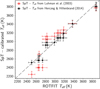 |
Fig. 3. Comparison between Teff estimates derived with ROTFIT for all targets and spectra, and Teff values corresponding to estimated SpT for each source (Table 2) using Luhman et al. (2003, red symbols) and Herczeg & Hillenbrand (2014, black symbols) calibrations. The x-axis uncertainties are those derived from the fit; the y-axis uncertainties correspond to half the difference in Teff between consecutive spectral subclasses in the corresponding SpT–Teff scale. The identity line is dashed in gray to guide the eye. |
3.1.3. Stellar mass, radius, and Ṁacc
Figure 4 shows the HR diagram populated by our targets5, using the L⋆ values reported in Table 2, and the Teff values associated with our SpT estimates following the scale of Herczeg & Hillenbrand (2014). A comparison between the location of the sources on the diagram and theoretical model isochrones, illustrated in the left panel of Fig. 4, would suggest that our sample spans the age range between 1–2 Myr and 10 Myr. This picture would also indicate that TWA 22 and TWA 31, whose membership to the TWA has recently been challenged (see Sect. 2), are slightly older than the bulk of TWA members.
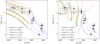 |
Fig. 4. HR diagram for stars in Table 2 (black dots) compared with disk–free TWA objects investigated in Manara et al. (2013b) and Stelzer et al. (2013) (gray diamonds), rescaled to Gaia DR2 distances and Herczeg & Hillenbrand’s (2014) SpT–based Teff. Filled symbols identify probable TWA members, open symbols targets with disputed membership. Errors on Teff and log L⋆ are as in Fig. 3 (y-axis) and Fig. 2 (x-axis), respectively. Left panel: theoretical isochrones from different model grids (Baraffe et al. 2015, dotted blue line; Siess et al. 2000, dash-dot red line; Tognelli et al. 2011, dashed green line; Spada et al. 2013, solid black line; Spada et al. 2017, solid yellow line) are shown for comparison on the diagram. The illustrated isochrone ages are, from top to bottom, 1 Myr, 2 Myr, 5 Myr, 20 Myr, and 100 Myr (the isochrones at 1, 2, and 5 Myr are not available from the models of Spada et al. 2013, and the 5 Myr isochrone is not available from the models of Spada et al. 2017). Right panel: mass tracks from the same model grids are illustrated for comparison. Displayed masses are, from right to left: 0.01 M⊙, 0.02 M⊙, 0.05 M⊙, 0.1 M⊙, 0.2 M⊙, 0.4 M⊙, and 0.6 M⊙ (Baraffe et al. 2015); 0.1 M⊙, 0.2 M⊙, 0.4 M⊙, 0.6 M⊙ (Siess et al. 2000; Spada et al. 2013); 0.2 M⊙, 0.4 M⊙, 0.6 M⊙ (Tognelli et al. 2011; Spada et al. 2017). |
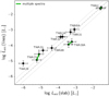 |
Fig. 5. Comparison between log Lacc values measured from excess continuum–fitting with slab emission models (Sect. 3.1.1), and values derived from emission line luminosity (Lline) measurements, using empirical Lline − Lacc calibration relationships from Alcalá et al. (2014). Error bars on the x-axis correspond to a typical uncertainty of 0.25 dex on the Lacc measurements from the multicomponent spectral fit; error bars on the y-axis follow from error propagation including uncertainties on the measured line fluxes, and uncertainties on the calibration relationships, as listed in Alcalá et al. (2014). Green lines connect multiple measurements for the same object. Light dotted lines delimit an area of ±0.3 dex around the equality line (dashed in gray on the diagram). |
Taken at face value, the data in Fig. 4 (left) appear inconsistent with a quoted age of 10 Myr for the TWA, which seems to be rather an upper limit to the age distribution of stars belonging to the association. This property appears to be shared by the sample of disk-free TWA members investigated with the same method in Manara et al. (2013b) and Stelzer et al. (2013), shown here for comparison purposes. Disk–free objects might tend to exhibit older ages than our targets, but a statistically significant comparison is hampered by the small number of objects and by the incompleteness of the sample (based on Gagné et al.’s 2017 census, only ∼25% of the disk–free stars in the TWA are shown in Fig. 4). Several studies (e.g., Hillenbrand et al. 2008; Pecaut & Mamajek 2016) have also shown that lower-mass stars tend to appear younger on PMS isochrone grids than higher-mass stars. This bias may amount to an artificial increase in logarithmic age by ∼0.7 dex over 1 dex in log M⋆ for solar-type stars at ages of a few Myr (Venuti et al. 2018), although those studies do not typically extend below M⋆ ∼ 0.2 − 0.3 M⊙, and the effect is not necessarily seen in our Fig. 4. On the other hand, a clear Teff–dependent age trend, with cooler objects in the very low-mass and brown dwarf regime appearing younger than earlier-type M-stars, is seen on the log g vs. Teff diagram in Fig. B.3, which also suggests a typical age for the TWA older than indicated on the HR diagram.
However, Fig. 4 also shows that the absolute age calibration is somewhat dependent on the model grid. This point is well discussed in Herczeg & Hillenbrand (2015), who illustrate in particular how different model grids applied to the same sample of TWA members can yield disparate age estimates between 5 and 10–15 Myr. Different ages proposed by different authors in the literature may also be affected by the limited number of objects included in each study. In addition, as shown in Fig. 4, most model tracks do not cover the region at the youngest ages and at the lowest M⋆ (≤0.1 M⊙), where it appears that small uncertainties in L⋆ would correspond to significant uncertainties on the individual age estimate (i.e., on the order of, or larger than, the age estimate itself). One of our TWA targets, J1247-3816, would seem significantly older than the others based on its location on the HR diagram (log L⋆[L⊙] ∼ −3); this is one of the two sources for which no solution could be determined via the multi-component fit (see Sect. 3.1.1), hence its L⋆ estimate may be subject to a larger uncertainty. The other source without multi-component fit solution (TWA 40) appears to be the youngest and lowest-mass object of the sample on Fig. 4; also in this case the position of the source on the HR diagram may be affected by a larger uncertainty than those of other targets.
For the reasons discussed above, we did not attempt a detailed analysis of individual ages for stars in our sample. Mass tracks from different model grids, instead, appear to be in overall agreement across the region of the HR diagram where they overlap (Fig. 4, right). We therefore estimated individual stellar masses via interpolation between theoretical mass tracks on the diagram, as detailed in the following. To ensure a uniform analysis across our sample, we adopted the set of models by Baraffe et al. (2015), which cover the entire mass range spanned by our targets, as illustrated in Fig. 4. We used the Teff and L⋆ values of the sources to interpolate their age along the isochrone grid: first, from the Teff coordinate we extracted the corresponding  along the two closest isochrones to the object’s location on the diagram; then, we interpolated between these two
  –age points to determine the age corresponding to the measured L⋆. We then used the derived value of age to extract the corresponding
  along the two closest mass tracks to the object’s location on the HR diagram, and the actual stellar Teff was used to interpolate between the resulting
  points to derive the final estimate of M⋆ for our target. Stellar radii (R⋆) were calculated using the Stefan-Boltzmann law.
The derived M⋆ and R⋆ parameters are reported in Table 2. These were in turn used, together with the Lacc from the multi-component fit, to compute the accretion rate onto the star, Ṁacc, as in Gullbring et al. (1998):
 (1)
(1)
where G is the gravitational constant. This procedure could not be adopted for J1247−3816 and TWA 40, which lack an Lacc measurement from the multi-component fit. For these two objects, an average estimate of Lacc was derived from the measured luminosities of several emission lines, as described in detail in Sect. 3.2.1. This procedure, which was applied to the entire sample as a consistency check for accretion parameters determined from different diagnostics, allowed us to obtain an estimate of Ṁacc for J1247−3816, and to set an upper limit for the Ṁacc on TWA 40, for which we did not detect any line emission. These two independent measurements of Ṁacc derived for all of our targets are also reported in Table 2.
3.2. A picture of accretion in the TWA
In this section, we compare different spectral indicators of accretion for our targets (Sect. 3.2.1) and we discuss the accretion properties derived as a function of stellar mass across the TWA (Sect. 3.2.2).
3.2.1. Continuum excess luminosity versus line luminosity
As mentioned earlier, the intense line emission produced by the heated gas in the accretion columns represents a widely used tracer of accretion, notably because such emission lines (e.g., Hα, Hβ) are more easily detected than the continuum excess luminosity on lower-mass stars and weaker accretors (e.g., Muzerolle et al. 2003). Line emission provides a more indirect diagnostics of accretion onto the star than the excess emission from the accretion shock itself, as the observed line luminosities and line profiles may also bear the imprints of magnetospheric outflows of material, as well as stellar chromospheric activity. Nevertheless, as shown in Herczeg & Hillenbrand (2008) and then in Alcalá et al. (2014), the luminosities (Lline) of several emission lines of H, He, and Ca correlate well with the values of Lacc, measured simultaneously from the spectral excess continuum emission. The derived empirical calibrations between the two quantities can therefore be used to extract an estimate of Lacc and, hence, Ṁacc from the measured Lline for individual objects (see also Frasca et al. 2017). In turn, this provides a cross-check for the accretion properties estimated on a given star from the observed excess continuum: disagreements between the two approaches may be symptomatic, for instance, of sources seen close to edge-on, where the visibility of the various accretion diagnostics may differ from case to case (e.g., Alcalá et al. 2014; Sousa et al. 2016).
In Fig. 5, Lacc measurements inferred from fitting the hydrogen slab model to the continuum excess emission are compared to the typical Lacc estimates ( ) derived from line emission diagnostics. Namely, the dereddened luminosities of several emission lines (H11, H10, H9, H8, Ca II λ3934, He I λ4026, Hδ, Hγ, Hβ, He I λ5876, Hα, and Paβ), when detected, were converted to Lacc using the relationships of Alcalá et al. (2014)6. The final
  (lines) estimate for a given object was then calculated as the median of all individual Lacc measurements from the detected emission lines, which are reported in Appendix E. A good fraction of the points on Fig. 5 are consistent, within the uncertainties, with a range of 0.3 dex around the identity line on the diagram, which corresponds to the rms scatter around the same identity line measured for the Lupus population. This suggests that the empirical Lacc − Lline calibrations determined by Alcalá et al. (2014, 2017) for the younger Lupus cluster can also be applied to derive a global picture of accretion in older PMS populations like the TWA. A few objects exhibit, however, a more conspicuous discrepancy between the different Lacc diagnostics. In the region of the diagram at log Lacc < −4, we observe two outliers (from left to right, TWA 28 and TWA 22) that fall above the diagonal strip (i.e., their Lacc estimated from the emission lines is significantly larger than their Lacc estimated from the Balmer continuum; a marginal discrepancy is observed for TWA 27).
It is interesting to note that all sources that populate the lower Lacc end of the distribution (hence presumably more evolved with respect to other accreting stars in our sample) share the property of being located above the identity line on the diagram, although in some cases being marginally consistent with the latter within the uncertainties. We speculate that, at lower accretion regimes, the emission lines may suffer a larger contamination from chromospheric activity, and therefore yield artificially higher values of Lacc than the measurement from the Balmer continuum. This effect would be especially pronounced on stars that rotate faster with respect to other accreting members, either at the end of magnetic braking or as a result of initial conditions at different stellar masses (Bouvier et al. 2014; Scholz et al. 2018; Moore et al. 2019), and therefore exhibit an enhanced chromospheric activity. Unfortunately, we could not find any estimate of rotation period reported in the literature for the two main outliers in this group to test this hypothesis, and the v sin i measurement that we have are rather uncertain. However, we note that the rotation period of 0.78 d measured by Lawson & Crause (2005) for TWA 8B, which lies at the upper end of the low log Lacc tail of objects on Fig. 5 (log Lacc [L⊙]∼ − 4), projects this object among the fastest rotators in the TWA (see also Messina et al. 2010). Some discrepancy at the lowest Lacc may also be symptomatic of less robust Lline–Lacc calibrations at these luminosity regimes, underrepresented in the Lupus sample (see Figs. C.5 and following in Alcalá et al. 2014) and where the relative contribution of chromospheric emission is more important. In addition, small differences between Lacc (slab) and Lacc (lines) might also be accounted for by the uncertainties associated with the best-fit stellar parameters.
In the area of the diagram at higher Lacc (log Lacc [L⊙]> − 4) we observe one star, TWA30 A, located below the diagonal strip (i.e., with Lacc estimate from the Balmer continuum larger than that derived from the line emission). This object is reported to be observed in a near edge-on configuration, although not fully edge-on (Looper et al. 2010). In this case, depending on the system geometry, it might occur that the regions where the line emission is mostly formed (e.g., the accretion funnels) are more occulted by the disk than the accretion shock at the star surface, thus determining the imbalance between the two approaches.
Figure 6 shows the distribution in  ratios as a function of stellar Teff, where
  is computed from the measured Lline. The diagrams also show the Teff-dependent “chromospheric noise limit” estimated for PMS stars. This corresponds to the amount of accretion luminosity that could be simulated by a non-accreting young star at the corresponding Teff or SpT, as a result of its chromospheric activity (see Sect. 3.2.2). This limit was calculated following the prescription of Manara et al. (2013b; see also Manara et al. 2017b), which was calibrated by measuring the luminosity of several emission lines, typically used as accretion tracers, on a sample of disk-free X-shooter targets in Lupus, σ Ori, and TWA. The line traces the approximate emission level below which the contribution from stellar chromospheric activity may become predominant in the observed line profiles. Conversely, stars projected well above this threshold on the diagram can be confidently assumed to be accreting. We stress that this threshold provides only an indication of where the transition occurs: as shown in Manara et al. (2013b), the sample of objects from which the calibration was drawn exhibit a scatter of ±0.2 dex in
  around the best-fitting line. Moreover, while a clear-cut boundary may be traced between strongly accreting objects and disk-free objects, this is likely not the case for weakly accreting objects, which can formally swing across the accreting vs. non-accreting threshold (e.g., Cieza et al. 2013).
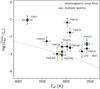 |
Fig. 6. Logarithmic ratio between median Lacc measured from Lline (see text) and stellar L⋆, as a function of Teff. Green vertical lines connect multiple measurements obtained for objects with more than one spectrum. The gray dashed line indicates the emission level below which the impact of chromospheric emission on the observed accretion signatures becomes dominant. |
Many of the stars in Fig. 6 fall above the chromospheric noise limit on the diagram, albeit by a smaller margin than observed in younger X-shooter regions (roughly half of them fall within 0.5 dex of the limit in  , whereas more than half of the Lupus targets in Alcalá et al. 2014 fall over 1 dex above the threshold). The same caveat mentioned earlier regarding the applicability of the Lline–Lacc calibrations at the lowest Lacc regimes holds here; however, we note that for at least two of the lowest Lacc objects (TWA 27 and TWA 28), an accreting nature is also suggested by their Hα flux following the criteria and empirical boundary for non-accreting objects derived by Frasca et al. (2015, Figs. 11 and 12) on the Chamaeleon I (3 Myr) and γ Velorum (5–10 Myr) populations. Two objects (TWA 30A and TWA 30B), instead, exhibit
  measurements consistent with the chromospheric noise threshold in Fig. 6. These two stars are known to be seen in a close to edge-on configuration (near edge-on but not fully edge-on for TWA 30A; fully edge-on for TWA 30B; Looper et al. 2010); it is therefore plausible that their accretion features are partly concealed from view, resulting in a low apparent accretion activity. In these cases, the measured Lacc should therefore be interpreted as a lower limit to the true level of accretion. The presence of forbidden emission lines in the spectra of both stars (see Sect. 3.3.2), on the other hand, indicates an active circumstellar environment with outflows of material.
3.2.2. The Ṁacc–M⋆ distribution
Figure 7 illustrates the distribution of Ṁacc as a function of M⋆. The accretion rates shown are the estimates derived from the continuum excess emission (Sect. 3.1.1), when available; these are complemented by the values derived from the line emission diagnostics (Sect. 3.2.1) for J1247−3816 and TWA 40 (upper limit). To estimate the mass-dependent, minimum Ṁacc we expect to be able to measure above the chromospheric noise on our targets, we followed the approach of Manara et al. (2013b, 2017b) applied to the model tracks of Baraffe et al. (2015). Namely, we took the Teff-dependent chromospheric noise limit illustrated in Fig. 6, and converted it to a range of Ṁacc by using the mass-dependent stellar parameters (L⋆, R⋆, Teff) tabulated in the theoretical models from Baraffe et al. (2015) that span the region of the HR diagram covered by our targets in Fig. 5. The result of this computation is shown as a shaded gray strip, which covers the approximate range in chromospheric emission expected, at a given mass, from stars aged between the average projected age of our targets on the HR diagram in Fig. 5 (∼3–5 Myr), and the upper estimate of 10 Myr for the nominal age of the TWA. The mass–dependent values of the Ṁacc noise threshold at an age of 10 Myr, calculated using Baraffe et al.’s (2015) models, are also reported in Table 3. The location of the Ṁacc noise threshold on the diagram in Fig. 7 is dependent, to some extent, on the specific model grid adopted for the conversion. However, a quantitative evaluation of the impact that this may have on the classification of our potential accretors is hampered by the fact that most sets of models do not cover M⋆ below ∼0.1 M⊙, as illustrated in Fig. 4. A comparison between the minimum Ṁacc obtained, as a function of M⋆, using alternatively the isochrones by Baraffe et al. (2015) and Siess et al. (2000) suggests differences on the order of 0.15 dex for M⋆ ∼ 0.1 − 0.7 M⊙. Such margin of uncertainty would not alter our selection of potential accretors above the noise threshold in Fig. 7.
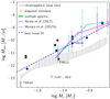 |
Fig. 7. Ṁacc vs. M⋆ distribution for stars in our sample, where Ṁacc is calculated from the measured continuum excess luminosity for all objects (filled dots) except TWA 40 and J1247−3816 (empty dots). Smaller red dots mark the locations of TWA 31 (upper point) and TWA 22 (lower point). Green vertical lines connect multiple Ṁacc measurements for the same objects. The shaded gray area traces the estimated chromospheric noise limit for Ṁacc detection, as a function of stellar mass, for stars aged between 3 and 10 Myr on Baraffe et al.’s (2015) isochrone grid. The dash-dot cyan line traces the bimodal Ṁacc − M⋆ relationship derived by Manara et al. (2017a) in the Chamaeleon I star-forming region, with a break at M⋆ ∼ 0.29 M⊙. The solid magenta line traces the bimodal relationship derived in Alcalá et al. (2017) in Lupus, assuming a break at M⋆ = 0.2 M⊙. Double arrows mark the 10th–90th percentile range in Ṁacc covered by the Lupus (magenta) and Chamaeleon I (cyan) populations as a function of mass. The dotted blue line traces a linear fit to the datapoints, which accounts for objects dominated by chromospheric emission (labeled on the diagram) as upper limits. |
Mass–dependent values of Ṁacc noise threshold, computed for stars at an age of 10 Myr using the models of Baraffe et al. (2015).
Three of our sources (from left to right, TWA 40, J1247-3816, and TWA 22) fall onto or below the estimated chromospheric noise limit. We therefore conclude that no significant accretion activity was detected for these sources. The star TWA 3A would fall above the semi-empirical Ṁacc noise threshold in Fig. 7, but we consider the corresponding Ṁacc as an upper limit rather than a true detection for the reason explained in Sect. 3.1.1. The remaining sources (8/12, excluding TWA 30B), however, exhibit some accretion activity. The measured Ṁacc show a dependence on the stellar mass. Following Venuti et al. (2014), we performed a Kendall’s τ test for correlation (Feigelson & Babu 2012; Helsel 2012) to assess the presence of a correlation trend and determine the quantitative relationship taking into account the upper limits (values consistent with the chromospheric noise threshold, labeled in Fig. 7) as censored data. Assuming a single power-law description, we obtained a best-fitting trend  with a significance of 2.5σ. This result is consistent with the relationships reported in the literature for younger clusters, albeit with a larger uncertainty that reflects the low number statistics of our sample and the sparse distribution on the diagram. The paucity of objects with M⋆ ≳ 0.3 M⊙ in our sample prevents any statistical comparison with the Ṁacc measured at those masses in younger regions. However, the levels of accretion observed on very low-mass stars and brown dwarfs in the TWA are similar in value and range to those derived with X-shooter among Lupus and Chamaeleon I stars. A more thorough discussion of these results in the context of Ṁacc evolution is reported in Sect. 4.1.
Recently, Manara et al. (2017a) and Alcalá et al. (2017) explored the possibility of a double power-law to reproduce the observed Ṁacc–M⋆ distribution in the Chamaeleon I and Lupus regions, respectively, using the same type of data and analysis adopted here. They showed that, in both cases, a double power-law, with a break around M⋆ ∼ 0.2 − 0.3 M⊙ and a steeper relationship in the lower-mass regime than in the higher-mass regime, provides a better statistical description to the observed data than a single power-law, although the latter cannot be excluded. This bimodal behavior, tentatively observed also in accretion surveys of other star-forming regions using different methods (e.g., Fang et al. 2013b; Venuti et al. 2014), has been predicted theoretically as an outcome of the early evolution of circumstellar disks governed by self-gravity and turbulent viscosity (Vorobyov & Basu 2009; other possible explanations of this bimodal trend are discussed in Manara et al. 2017a). The bimodal power law determined in Manara et al. (2017a) (break at M⋆ ∼ 0.29 M⊙) and that computed in Alcalá et al. (2017) (break at M⋆ = 0.2 M⊙) are both traced for comparison in Fig. 7. Objects in our sample do not provide sufficient parameter coverage to assess whether a bimodal or a unimodal distribution describes the observations better. We simply note that the extrapolation of Manara et al. and Alcalá et al.’s relationships (calibrated down to log M⋆ [M⊙]∼ − 1.1) does not appear to match the observed accretion properties of the lowest–mass objects in the TWA, although both descriptions could fit the data above log M⋆ [M⊙]∼ − 1.3. This is consistent with indications from Manara et al.’s (2015) study of accretion in very low-mass stars and brown dwarfs in the 1–2 Myr-old ρ Ophiucus, with measured Ṁacc that would fall well above the predicted Ṁacc at the lowest–mass regimes in the broken power-law description of Manara et al. (2017a) and Alcalá et al. (2017).
We note that cases of objects near the brown dwarf regime with Ṁacc higher than expected based on the M⋆ − Ṁacc trend for M⋆ ≃ 0.1 − 0.3 M⊙ stars were also observed in Lupus. Overall, these data hint at a different behavior of accretion at the lowest stellar masses. Alcalá et al. (2017) proposed that these objects could be understood in the theoretical framework of Stamatellos & Herczeg (2015), according to which the lowest-mass stars do not form via prestellar core collapse, but as a product of the fragmentation of disks around solar-mass stars. In this scenario, the disk that takes shape around the newly formed substellar object continues to accrete material from the parent disk before starting to evolve independently. This process leads to comparatively more massive disks, relative to the mass of the central object, than those formed via prestellar core collapse, which translates to comparatively higher accretion rates onto the star. On the other hand, Testi et al. (2016) used ALMA data to report tentative indications of a lower Mdisk/M⋆ ratio for brown dwarfs than for solar-mass stars in ρ Oph, albeit potentially affected by sample incompleteness and large uncertainties on the stellar parameters adopted.
3.3. Emission lines as tracers of the star-disk interaction environment
In this section, we explore the strength and morphology of permitted emission lines in the Balmer series (Sect. 3.3.1) and of the forbidden line [O I] 6300 Å (Sect. 3.3.2) to probe the physical conditions of the inner circumstellar environment.
3.3.1. Hα line profiles and Balmer decrements
The profiles of several emission lines, in particular Hα and others from the Balmer series, have long been investigated in the literature in connection with the physical conditions of the circumstellar environment in PMS stars. In their seminal work, Reipurth et al. (1996) established a first thorough classification of Hα line profiles in young stars. The authors identified four main types (Type I–IV) of Hα morphologies, related to the dynamics of material infall or ejection that takes place in the inner disk regions. We here applied Reipurth et al.’s (1996) classification to sort our Hα line profiles empirically based on their shapes. In addition, we implemented a simple Gaussian description to evaluate the deviation of the individual lines from a symmetric profile. Details of this analysis are reported in Appendix C, and the main inferences are summarized in the following paragraph.
While none of the observed line profiles appears strictly Gaussian, a Gaussian description appears adequate to describe the global Hα profile observed on around 50% of the targets. Overall, 50% of the Hα profiles in our sample fall into the Type I class definition (symmetric, with no absorption features); Type II profiles (double-peaked) occur in 37.5% of cases, while smaller percentages are associated with the Type III (8.3%) and Type IV (4.2%) classes. This distribution is similar to those found by Antoniucci et al. (2017) in Lupus and Sousa et al. (2016) in NGC 2264, both aged around 3 Myr. Antoniucci et al. (2017) also classified the observed Hα profiles in the Lupus region based on their FWHM, and identified two similarly populated, distinct groups: narrow-line objects, with FWHM ≲ 100 km s−1, and wide line profiles, with FWHM ∼ 200–300 km s−1. Our sample is distributed in a different way than the Lupus sample in this respect: the majority of objects (83%, including those where chromospheric activity is possibly predominant) are found in the narrow-line group, while only TWA 1 and the disputed member TWA 31 exhibit wide line profiles with FWHM ∼ 200–250 km s−1.
In the context of the X-shooter survey of the Lupus star-forming region, Antoniucci et al. (2017) also undertook a detailed analysis of the Balmer decrements, that is, of the ratio of fluxes between different HI emission lines in the Balmer series, exhibited by accreting stars in the region. As shown in their article (see in particular their Table 3), the decrement shapes can be related to the physical properties (e.g., density, temperature) of the emitting gas. Antoniucci et al. (2017) identified four main types of Balmer decrements, defined by the value of log FH9/FH4 (henceforward logH9/H4). The different decrement shapes observed were found to correspond to different predictions of the local line excitation calculations by Kwan & Fischer (2011), which describe line emission under varying physical conditions of winds and accretion flows in T Tauri stars. In Fig. 8, we illustrate the Balmer decrement shapes computed for our targets, compared with the prototypes of the four Balmer decrement types identified in Lupus by Antoniucci et al. (2017). The luminosities of the Balmer lines from Hα to H15 that we measured for our targets are reported in Table E.1. The Balmer line ratios were computed taking as reference the luminosity of the H4 (Hβ) line, in analogy with the definition of Antoniucci et al. (2017). Most of the nine objects with measured H9-to-H4 ratio in our sample (83%) fall into the type 2 category of Balmer decrement shapes, as defined by Antoniucci et al. (2017), which can be associated with total gas densities log nH ∼ 9.5 and temperatures in the range 5000–15 000 K. This result is similar to the one reported in Lupus (type 2 being the most common category of Balmer decrement shapes), but with a larger rate of occurrence than the 56% found in that case. One object (TWA 28) exhibits a type 1 Balmer decrement profile (11%). This rate, albeit subject to our very limited statistics, is similar to the one found by Antoniucci et al. (2017) in Lupus. We could not establish from the literature whether TWA 28 is also an edge-on system like the Lupus objects that exhibit type 1 Balmer decrement profiles. We note, however, that TWA 28 is the source with the largest discrepancy between  (lower) and
  (higher) in Fig. 5, which might be consistent with a geometry where the central region of the star is more obscured than the line-emitting region. Another object (TWA 27) exhibits a type 2 Balmer decrement at one epoch (P089), and a type 3 Balmer decrement in another epoch (P084). We did not detect any strong variations in the Hα FWHM, and measured a variation of only ∼0.15–0.25 dex in Ṁacc between the two epochs, which is consistent with the typical week-long (that is, on rotational timescales) accretion variability monitored on young stars at ages of a few Myr (e.g., Costigan et al. 2014; Venuti et al. 2014; Frasca et al. 2018). However, TWA 27 exhibits stronger Hα emission in P089 than in P084, but stronger Hβ emission in P084 than in P089. We note that this object had been the target of detailed spectroscopic monitoring by Stelzer et al. (2007), who reported generally multi-structured Balmer line profiles, with variations in the shape and relative intensity of the peaks on timescales ranging from hours to months. Evident variations in the Hα line morphology for TWA 27 are also observed between our two epochs, as illustrated in Fig. C.1.
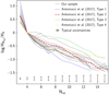 |
Fig. 8. Shapes of Balmer decrements computed for each of our targets (gray lines), defined as logHn/H4 (≡logHn/Hβ). The prototypes of Balmer decrement types identified in Lupus by Antoniucci et al. (2017) are shown with dotted lines for comparison; a thicker stroke is used to emphasize Type 2 (the most common type in their sample and in ours). Typical uncertainties on the log HNup/H4, displayed below the individual Balmer decrement trends, were calculated from the uncertainties associated with the corresponding line flux measurements. |
We did not find any straightforward correlation between the Balmer decrement type and the Hα line shape or the Ṁacc level; the typical logH9/H4 in each Hα class and Ṁacc bin falls always in the type 2 Balmer decrement category, but there might be a tendency for Type II Hα profiles to correspond to slightly larger logH9/H4, and for the strongest accretors in our sample to exhibit slightly smaller logH9/H4. Following Antoniucci et al.’s (2017) interpretation, the typical Balmer decrement properties observed may indicate that stars in the TWA are accreting at a moderate regime with optically thin emission. None of our targets with Balmer emission lines detected until the order 14 have Balmer decrements of type 4, which were associated by Antoniucci et al. with wide Hα line profiles, intense accretion activity, and optically thick emission. However, we did detect two objects (TWA 1 and TWA 31) with large Hα FWHM, as discussed earlier; these two objects exhibit the largest Ṁacc measured at the corresponding M⋆ in our sample.
For stars in Lupus, Frasca et al. (2017) also investigated the line flux ratios in the Ca II infrared triplet (IRT), which are used as tracers of both chromospheric activity and accretion, and likely probe the physical conditions of the emitting gas in a region closer to the photosphere than what traced by the Balmer lines. In our sample, Ca II 8498 Å and Ca II 8542 Å emission was only detected for seven objects (TWA 1, TWA 8A, TWA 28, TWA 30B, TWA 31, and TWA 32, plus the object TWA 3B discussed in Appendix A). In all of the cases where Ca II IRT emission was detected, the measured flux ratios are consistent with optically thick emission that may originate in accretion shocks or chromospheric plages, as illustrated in Fig. E.1.
3.3.2. Accretion and ejection activity: outflow signatures
Mass accretion processes in PMS stars are interconnected with mass ejection phenomena, such as magnetically powered jets and disk winds. These mechanisms play a crucial role in removing angular momentum from the system, which in turn allows disk material to be transported inward and accrete onto the star. Jets and winds in young stellar objects (YSOs) are revealed spectroscopically by the presence of forbidden emission lines, which are excited in the heated high-velocity gas. Such lines often exhibit a complex profile with multiple components (e.g., Rigliaco et al. 2013; Simon et al. 2016; McGinnis et al. 2018; Banzatti et al. 2019): a low velocity component (LVC), centered close to the system velocity and possibly associated with slow disk winds (e.g., Natta et al. 2014), and a high velocity component (HVC), shifted by up to ∼200 km s−1 with respect to the stellar rest frame, and associated with extended collimated jets (e.g., Nisini et al. 2018).
The [O I] 6300 Å is the most intense among the forbidden emission lines observed in YSOs. As part of the X-shooter Italian GTO survey of star-forming regions, Natta et al. (2014) and Nisini et al. (2018) recently investigated the connection between the luminosity of the LVC and the HVC of the [O I] 6300 Å line, and the stellar and accretion parameters derived simultaneously and homogeneously for YSOs in Lupus, Chamaeleon, and σ Ori. Following their approach, we here analyzed the [O I] 6300 Å emission properties for stars in the older TWA, to test any evolutive trends in the relationships reported by those authors. We identified [O I] 6300 Å emission above the local continuum in four sources: TWA 1 (both spectra), TWA 30A (all spectra and epochs), TWA 30B (both epochs), and disputed member TWA 31. Our rate of detection is therefore 4/13 objects (∼31%) across our entire sample, and 3/11 (27%) including high-likelihood TWA members only. This percentage is lower than the 77% found in Nisini et al. (2018), and than the 59% reported by McGinnis et al. (2018) in a similar study conducted with VLT/FLAMES on the NGC 2264 region (3–5 Myr). Even higher rates of detection were reported by Simon et al. (2016) in Taurus (91%, based on 32 disk-bearing objects), and by Banzatti et al. (2019, 94%) in a composite sample of 65 objects from different star-forming regions and PMS associations.
To recover the LVC and HVC, we performed a Gaussian fit to the observed line profile, after normalizing the flux to the local continuum and subtracting the photospheric contribution to the line emission. In the formulation of Eq. (C.1) (where a is fixed to 1), we explored a range of values for k, μ, and σ, and for each of them we evaluated the goodness-of-fit via the χ2 statistics. We then repeated the analysis assuming two Gaussians, and selected the best solution (single line component or two line components) as the one with the smallest reduced χ2. The results of this procedure are illustrated in Fig. 9. In half of the cases (both spectra of TWA1, TWA30 A_P087, and TWA 31) we could only identify a LVC; we instead extracted two separate components (LVC plus a blueshifted HVC) from the [O I] 6300 Å line profile exhibited by TWA 30A_P087 (both spectra) and TWA 30B (both epochs). The extracted luminosity values for both components are reported in Table D.1. Our rate of detection of a HVC is therefore 2/13 (15%) across the entire sample, and 2/11 (18%) for TWA only. For comparison, Nisini et al. (2018) reported a HVC for 30% of their targets in Lupus, Chamaeleon I and σ Ori, while McGinnis et al. (2018) detected HVCs in 17% of their targets in NGC 2264.
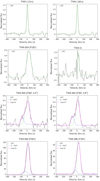 |
Fig. 9. Best single-Gaussian (LVC) or double-Gaussian (LVC+HVC) solution obtained for the [O I] 6300 Å line profile decomposition of TWA 1, TWA30 A, TWA 30B, and TWA 31. The LVC is traced with a dotted green line, the blueshifted HVC (when present) is traced as a dotted blue line, and the total fit is traced as a dotted magenta line. |
Figure D.1 shows the comparison between the luminosity measured for the [O I] 6300 Å LVC in the four objects listed above, and the corresponding stellar (L⋆, M⋆) and accretion (Lacc, Ṁacc) parameters. A statistically meaningful comparison with earlier results is prevented by the very small number of objects with [O I] 6300 Å emission in our sample. We can simply observe that the distribution of points derived here on each panel in Fig. D.1 is globally consistent with the prescriptions obtained by Nisini et al. (2018) and Natta et al. (2014), within the dispersion about the best fitting relationships measured for the Lupus, Chamaeleon, and σ Ori populations (see Figs. 4 and 6 of Nisini et al. 2018).
4. Discussion
4.1. The evolution of disk accretion between ∼1 and 10 Myr
Figure 10 summarizes the global accretion properties measured in the course of X-shooter campaigns on six PMS clusters and stellar associations of different ages: ρ Ophiuchi (Manara et al. 2015; age ∼0.5–2 Myr, Wilking et al. 2008), the previously introduced Lupus and Chamaeleon I (age ∼3 Myr, with a spread of 2 Myr), σ Orionis (Rigliaco et al. 2012; age re-estimated as  Myr by Bell et al. 2013), the η Chamaeleontis association (Rugel et al. 2018; age ∼11 ± 3 Myr, Bell et al. 2015), and the TWA investigated here (age ∼10 ± 3 Myr, Bell et al. 2015). In spite of the age controversy mentioned in Sect. 3.1.3, we adopt here the age estimates from Bell et al. (2013, 2015) for the older regions because they were obtained with a uniform approach, hence warranting at least a robust relative ordering in age. We note that, while the surveys of Lupus, Cha I and TWA are estimated to be ≳90% complete in the disk-bearing population of the targeted regions, the X-shooter surveys of ρ Oph and σ Ori specifically address the lowest mass component of the cluster populations (M⋆ ≲ 0.3M⊙), and the survey of η Cha encompasses around 68% of the suspected members of the association. To account for the different distributions in mass of each sample, we followed the approach of Rugel et al. (2018, see also Antoniucci et al. 2014), and show in Fig. 10 the median Ṁacc, normalized to
  , measured across each region. This normalization effectively removes the typical M⋆–dependence observed in the Ṁacc distributions of PMS populations (
 ; e.g., Hartmann et al. 2016), and therefore enables a comparison of the average accretion level as a function of cluster age as unaffected by the specific mass coverage as possible.
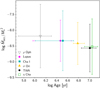 |
Fig. 10. Median age and accretion properties normalized to squared mass for six young regions targeted with X-shooter: ρ Ophiuchi (Manara et al. 2015; gray empty triangle), Lupus (Alcalá et al. 2014, 2017; magenta diamond), Chamaeleon I (Manara et al. 2017a; cyan square), σ Orionis (Rigliaco et al. 2012; yellow triangle), TWA (this study; black dot), and η Chamaeleontis (Rugel et al. 2018; green empty square). The horizontal error bars mark the measured age spread among cluster members in the case of ρ Oph, Lupus, and Cha I, and the uncertainty on the nominal age for σ Ori (Bell et al. 2013) and the associations TWA and η Cha (Bell et al. 2015). The vertical errors mark the logarithmic dispersion in |

Figure 10 seems to suggest a marginal decrease in Ṁacc with increasing age, the extent of which is, however, appreciably smaller than the 1σ scatter in value measured in any region. To assess the statistical significance of the apparent trend, we created 10 000 sets of  pairs, randomly extracted within the uncertainties illustrated in Fig. 10 assuming a uniform distribution in logAge and a Gaussian distribution in
  around the best values. For each set of simulated measurements, we computed the Pearson’s correlation coefficient r (e.g., Press et al. 1992); we then calculated the average and the standard deviation of the resulting r values as an indicator of the strength of the seeming anticorrelation trend, given the uncertainties. The distribution in r that we derived peaks around −0.2, with a standard deviation of 0.4; this result is not dependent on the number of simulated sets adopted, as the same parameters for the distribution in r are obtained when using 100 or 1000 iterations instead of 10 000. The test therefore indicates that, if we account for the uncertainties and for the intrinsic scatter in values within each population, we cannot conclude on whether a decrease in Ṁacc is actually observed on Fig. 10. Furthermore, the error bars displayed on the diagram do not include additional sources of uncertainty, such as the exact power of M⋆ that ought to be adopted to flatten the distribution in Ṁacc vs. M⋆ within a given population, or the different selection biases (for instance, the inclusion or exclusion of upper limits in Ṁacc) when computing the averaged statistics for each region.
Figure 11 illustrates the distribution of individual targets for the six regions presented in Fig. 10 on the Ṁacc − M⋆ diagram. A detailed quantitative analysis is hampered by the fact that the distributions in mass pertaining to the six samples are different from each other, and little can be said for the mass regime M⋆ ≥ 0.3 M⊙, where we have only one star from the TWA (TWA 1) and a few more from ρ Oph and η Cha, with measured Ṁacc below the median accretion level detected in the corresponding mass bin for the composite Lupus and Cha I sample (horizontal line in Fig. 11). At lower masses (M⋆ ∼ 0.08 − 0.25 M⊙), where the samples overlap, stars in ρ Oph appear located systematically above the Ṁacc levels measured in the other populations. However, this effect should be interpreted with caution since the accretion rates for ρ Oph targets were measured from the emission lines, contrary to the quasi-totality of other measurements shown on the diagram (which were derived from the Balmer continuum emission), and are subject to larger uncertainties (Manara et al. 2015). If we exclude ρ Oph, on the other hand, it appears that the remaining populations cover similar ranges in Ṁacc at the lowest stellar masses, with striking evidence for some 5–10 Myr-old accreting stars with measured Ṁacc higher than the typical level of accretion detected in the combined Lupus + Cha I sample. This comparison might be affected by different completeness limits of the various surveys over the mass range of intersection among the various samples (for instance, the Lupus surveys did not include many young star candidates with M⋆ ≲ 0.1 M⊙, and Manara et al. 2017a quote a completeness limit of SpT ∼ M6 for the Cha I sample). Nevertheless, the selection bias would impact predominantly the low Ṁacc regimes at the corresponding M⋆, and is unlikely to cause a dearth of stronger accretors in the mass range of interest for the two younger populations. The picture in Fig. 11 therefore suggests that very low-mass stars that still retain a disk at the age of the TWA can sustain a prolonged accretion activity with an Ṁacc possibly more “stable” (i.e., slowly evolving) in the long-term than on more massive stars. This may perhaps be related to a more efficient photoevaporation effect in dissipating material in the inner disks around higher mass stars.
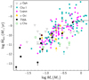 |
Fig. 11. Comparison between the Ṁacc − M⋆ distributions obtained from X-shooter data for ρ Ophiuchi, Lupus, Chamaeleon I, σ Orionis, TWA, and η Chamaeleontis (symbols and sources of data as detailed in the caption of Fig. 10). Upper limits in Ṁacc are marked by downward arrows. The horizontal lines mark the median Ṁacc measured in bins of 0.25 dex in log M⋆ for the combined Cha I and Lupus datasets. |
To ascertain whether this conclusion might be affected by the incompleteness of the X-shooter survey of disk–free PMS stars in the TWA (see Sect. 3.1.3), we examined the SpT distribution of all 55 high-likelihood members listed in Gagné et al. (2017) with reference to the presence or absence of accretion disk signatures. This analysis indicates that, while less than 10% of TWA stars with SpT between M0 and M3 exhibit such signatures, the percentage of accreting objects rises to ∼40% among M4–M9 stars. If the evolutionary timescales for disk accretion were the same for very low-mass stars and brown dwarfs (M⋆ ∼ 0.02 − 0.2 M⊙) as for higher-mass stars (M⋆ ∼ 0.2 − 0.6 M⊙), this result would imply that the lowest–mass objects in the TWA are statistically younger (i.e., they were formed at later epochs) than higher–mass objects in the same association. However, this scenario is not supported by the similarity in spatial and kinematic properties between low–mass stars and brown dwarfs in loose star–forming regions such as Taurus (Luhman et al. 2007).
We note that the mass regime (M⋆ ≤ 0.2 M⊙) where longer timescales for Ṁacc evolution appear to hold from our analysis lies below the typical mass range (M⋆ ∼ 0.3 − 1 M⊙) for which tentative Ṁacc(t) have been proposed in the literature following a multi-cluster approach (e.g., Hartmann et al. 1998, 2016; Calvet et al. 2005; Sicilia-Aguilar et al. 2010)7. Hartmann et al. (2006) speculated that low-mass disks around the lowest–mass stars might be viscously drained on shorter timescales, therefore yielding a stronger Ṁacc dependence on stellar age than observed on young stars of mass closer to 1 M⊙. In their analysis of accretion in the Orion Nebula cluster, Manara et al. (2012) combined individual Ṁacc and stellar age measurements to report a faster temporal decay of Ṁacc in very low-mass stars (M⋆ < 0.2 M⊙) than in more massive stars (M⋆ ∼ 0.4 − 1 M⊙). On the other hand, in a similar study of the NGC 2264 region Venuti et al. (2014) reported a looser correlation between Ṁacc and age for lower-mass stars (M⋆ < 0.4 M⊙) than for higher-mass stars (M⋆ ∼ 0.4 − 1 M⊙), although pointing out the uncertainty associated with model–based individual age determinations for young stars.
4.2. Connection between disk mass and mass accretion
The relationship between the mass accretion rate Ṁacc onto young stars and the mass of their circumstellar disks (Mdisk) is a key observational proxy to understand the leading physical processes in disk evolution. From a theoretical standpoint (see, e.g., Rosotti et al. 2017; Lodato et al. 2017), it is expected that, in a scenario where the disk has attained a quasi-steady state of viscous evolution, Ṁacc should be on the order of Mdisk over the age t of the star-disk system: Ṁacc ∼ Mdisk/t. Other processes that trigger an inside-out disk clearing (such as internal photoevaporation driven by the radiation from the central object) would determine a faster depletion of material from the inner disk region (where accretion takes place) than from the outer disk region; in this case, the theoretical expectation is Ṁacc < Mdisk/t. In the opposite scenario of outside-in disk clearing (which can be triggered by external photoevaporation by nearby massive stars), the disk mass decreases at a faster pace than can be accounted for by viscous accretion onto the star; in this case, Ṁacc > Mdisk/t (Rosotti et al. 2017). Recent studies (Manara et al. 2016; Mulders et al. 2017) have combined X-shooter measurements of Ṁacc with ALMA measurements of Mdisk to infer a correlation between the two parameters for young stars in Lupus and Chamaeleon I. The observed trend results compatible with the linear relationship predicted in the case of viscous disk evolution, albeit with a significant scatter that may reflect contributions from additional physical processes in the transport of material and angular momentum across the disk (grain growth and migration, disk winds), or viscous timescales longer than the average age of the regions (Lodato et al. 2017).
In Fig. 12 we compare the Mdisk − Ṁacc properties for TWA sources in our sample with the distributions reported for Lupus and Chamaeleon I. For consistency purposes, the values adopted for the latter two are those converted to individual Gaia DR2 distances and to Baraffe et al.’s (2015) models. For TWA stars, we adopted the estimates (or upper limits) of Mdisk, dust computed by Rodriguez et al. (2015) from ALMA observations, where available; the Mdisk, dust were converted to Mdisk assuming Mdisk ∼ 100 Mdisk, dust, as in Manara et al. (2016). The Mdisk shown for TWA 1 is taken from Trapman et al. (2017). With the exception of TWA 1, the TWA sources exhibit some evolution with respect to the populations of Lupus and Cha I, being located in the quarter of the diagram at low Ṁacc and low Mdisk. However, the vertical scatter among TWA members on the diagram is at least similar to that measured across the statistically larger Lupus and Cha I samples, rendering the comparison between the observed TWA properties and the theoretical viscous predictions very uncertain. J1247-3816 is the only object of the TWA subsample that exhibits a position on the diagram compatible with the expected locus for disks aged ∼10 Myr that have attained a viscous quasi-steady state. TWA 1 and TWA 32 lie roughly in the same strip traced by Lupus and Cha I members (i.e., above the viscous steady-state prediction at the nominal age of the association). TWA 30A and TWA 31 appear even above the assumed steady-state locus with a viscous timescale of 0.1 Myr, which crosses the upper envelope of the datapoints distributions pertaining to Lupus and Cha I. TWA 30A is, however, a nearly edge-on star-disk system, which may have introduced additional uncertainties on the measured parameters (see Sect. 3.2.1) and on the Mdisk derivation. As to TWA 31, its membership to the TWA has recently been disputed, as mentioned in Sect. 2.1, although the new classification would place this object at an older age than the TWA and, therefore, would render its position on Fig. 12 even more inconsistent with the predicted locus for viscously evolved disks.
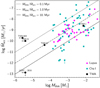 |
Fig. 12. Logarithmic Ṁacc vs. disk mass distribution for stars in the TWA, compared to the populations of the Lupus and Chamaeleon I star-forming regions. The straight lines mark the Ṁacc − Mdisk relationship predicted for different stellar ages in a scenario of viscous quasi-steady disk evolution (Rosotti et al. 2017). Upper limits are indicated by correspondingly oriented arrows. |
The scarceness of objects in our sample with definite measurements for Fig. 12 prevents us from drawing any robust conclusion from the comparison with Lupus and Cha I. What the overall picture appears to hint at is that a purely viscous disk evolution scenario is insufficient to explain all of the observations. This tentative inference is aligned with the conclusions of Ingleby et al. (2014), who compared observations of older (5–10 Myr) stars with significant accretion to the expected decline in Ṁacc with age from viscous evolution models, and showed that the latter cannot explain a prolonged accretion activity at the observed rates without assuming very high Mdisk that would render the disk unstable.
4.3. Impact of stellar mass and environmental conditions on Ṁacc evolution
Statistical studies of disk fractions in young star clusters as a function of stellar mass and age have suggested longer evolutionary timescales for disks surrounding lower-mass stars than those around higher-mass stars. Ribas et al. (2015) analyzed a large sample of stars from eleven young clusters and stellar associations of age between 1 and 10 Myr, to infer that lower-mass stars are statistically more likely to host a “protoplanetary” disk (i.e., a disk which produces an infrared excess at λ < 10 μm) than more massive stars at any given age between 1–3 and 10 Myr. However, the broad mass bins used in that study to define low-mass stars (M⋆ < 2 M⊙) and high-mass stars (M⋆ ≥ 2 M⊙) do not allow us to connect this picture with the slow Ṁacc evolution we infer for M⋆ < 0.3 M⊙ stars from the discussion in Sect. 4.1.
In their review on protoplanetary disk evolution, Williams & Cieza (2011) pointed out that the disk dissipation timescales for substellar objects appear to be at least comparable to, if not longer than, those pertaining to solar-like objects (SpT of K to early-M), with the caveat that the observational statistics available in the lowest-mass regime is significantly poorer than at higher masses. Nevertheless, some evidence of a mass-dependent disk fraction has been reported also among stars less massive than ∼1 M⊙ within a given cluster. Carpenter et al. (2006) employed Spitzer observations from 4.5 to 16 μm to assess the disk fraction of young stars in the Upper Scorpius region (∼8 Myr-old). They estimated a total disk fraction of 19% among K0–M5 stars, in contrast to ≲1% among massive stars in their sample. Their data also suggest an increasing disk fraction with later SpT among M-type stars themselves, as about 10% of early M-stars (< M3) were found to exhibit an infrared excess at 8 μm and 16 μm, while the percentage amounted to 20–30% among M4–M5 stars. Scholz et al. (2007) complemented that survey by investigating the disk fraction among young brown dwarfs in Upper Sco (SpT = M5–M9), using Spitzer data between 8–24 μm, and observed signatures of disks around 37%±9% of their targets. This value may be subject to a larger uncertainty than the estimates around higher-mass stars, perhaps reflecting completeness limits at the low-mass end of the cluster population, as suggested by the subsequent work of Riaz et al. (2009), who reported a disk fraction of  from their own sample of brown dwarfs in Upper Sco, and a combined disk fraction of
  from their and Scholz et al.’s (2007) studies.
More recently, Dawson et al. (2013) considerably expanded the census of very low-mass stars and brown dwarfs in Upper Sco, and derived a disk fraction (23%±5%) consistent with that estimated by Carpenter et al. (2006) for K0–M5 stars. On the other hand, Luhman & Mamajek (2012) examined multiple disk signatures at Spitzer and WISE wavelengths and reported a consistent increase in disk fraction with later spectral types, going from ∼10% for K-type stars to ∼20% in M0–M4 stars and ∼25% in M4–M8 stars. A definite increase in disk fraction with decreasing stellar mass in Upper Sco was also found by Cook et al. (2017), who focused in particular on the substellar mass regime and reported a disk frequency among M⋆ < 0.05 M⊙ objects about 2–3 times higher than among 0.05 − 0.15 M⊙ objects. The criteria adopted in each of these recent studies to build a census of substellar mass and brown dwarf members of the cluster (photometric association with the cluster sequence on optical and near-IR color-magnitude diagrams, kinematic association with the cluster, spectral indicators of youth) are independent of the presence or absence of a disk, which was assessed later using separate mid-IR data. Therefore, no significant biases against selection of low-mass stars without disks are expected to affect their inferences. Overall, these results provide a good statistical indication of a longer disk lifetime around very low-mass stars than around solar-mass objects. The slow evolution in Ṁacc that we observe in Figs. 10 and 11 for M⋆ ≲ 0.3 M⊙ stars between 3 and 10 Myr may be connected to the longer disk lifespans, although Scholz et al. (2007) found definite signatures of ongoing accretion only for around 30% of their targets with clear indications of inner dust disks (however, Scholz et al.’s sample includes objects with M⋆ < 0.1 M⊙, whereas the mass range where our comparison is best performed from the dataset in Fig. 11 lies between M⋆ = 0.1M⊙ and 0.3 M⊙).
Previous studies have also reported evidence for longer timescales of disk evolution in sparse stellar associations as opposed to compact or crowded clusters, where dynamical interactions with nearby objects may play a significant role. Fang et al. (2013a), in particular, examined the disk fraction vs. age relation for 19 star-forming regions and young stellar associations (including Cha I, σ Ori, Upper Sco, and the TWA) to derive the characteristic timescale τ0 for disk evolution. While the exact numbers are dependent on the specific age estimates for a given young stellar population (see discussion in Bell et al. 2013), the τ0 that they estimated from their sample of sparse associations, 4.3 ± 0.3 Myr, is significantly longer than the 2.8 ± 0.1 Myr measured for young star clusters (see also Fedele et al. 2010). The authors also inferred a tentative connection between the characteristic timescale of disk accretion and the sparseness of the stellar population, showing that at least the primary target of their investigation, the ϵ Cha association, hosts a significantly larger fraction of accreting stars than expected based on the accretion timescales estimated by Fedele et al. (2010) for their selection of clusters. More studies, combining the information on occurrence of disk-bearing and accreting objects as a function of age with accurate measurements of their accretion rates over a wide range of stellar masses and external conditions, are needed to fully elucidate the dynamics and drivers of accretion evolution in protoplanetary disks.
5. Conclusions
We have conducted a thorough spectroscopic study of disk accretion in the ∼5–10 Myr-old TWA, employing homogeneous data from the X-shooter spectrograph, and making use of well-established methods of reduction and analysis developed earlier during the Italian X-shooter GTO program on star-forming regions (Alcalá et al. 2011). Our survey encompasses eleven stars with IR signatures of circumstellar material in the TWA, plus two disk-bearing stars recently disputed as TWA members and suggested to belong to nearby PMS associations, and one TWA member with no evidence of dusty inner disk reported in the literature. Our targets account for ∼85% of the estimated population of young stars with disks in the TWA, they range in SpT between M0 and M9, and have masses between 0.58 M⊙ and 0.02 M⊙. We took advantage of the broad spectral window covered by X-shooter (from ∼300 nm to 2500 nm) to determine individual extinction, stellar parameters, and accretion parameters for each target simultaneously via multi-component fits to several features of the observed spectra. We then examined the shapes and relative strengths of the detected Balmer emission lines, and the detection rate and structure of the forbidden [O I] 6300 Å emission line, to probe the physical conditions of the accretion and ejection mechanisms at play.
The TWA offers a unique perspective into the final stages of the disk lifetimes around stars from subsolar masses to the brown dwarf regime, often inaccessible in more distant regions. We detected signatures of ongoing accretion activity above the chromospheric noise level for around 70% of our TWA targets (disk-bearing stars), which translates to a fraction of accretors of 13% to 17% across the whole TWA population (including both disk-bearing and disk-free objects). This fraction is significantly smaller than the frequencies of accreting stars typically detected in very young (< 3 Myr-old) PMS populations (∼40–50%), but larger than those measured for several > 5 Myr-old clusters in earlier studies (< 5–10%; see, e.g., Fedele et al. 2010 and references therein, and Frasca et al. 2015). Our analysis of the line emission detected on our targets indicates that some evolution has taken place with respect to younger star-forming regions investigated previously in a similar manner, most notably the 1–3 Myr-old Lupus. First of all, while the morphological classification of Hα profiles in the TWA is statistically similar to the distribution in profile types (Reipurth et al. 1996) found in younger regions (e.g., Lupus, NGC 2264), around 50% of our targets exhibit Hα lines with an overall Gaussian profile, and 83% exhibit narrow Hα lines (FWHM ≲ 100 km s−1). This percentage is significantly larger than the 44% narrow-line profiles found by Antoniucci et al. (2017) in Lupus. Furthermore, most of our targets (83%) exhibit Balmer decrements consistent with the most common class identified by Antoniucci et al. (2017) in Lupus (type 2, corresponding to moderate accretion regimes with optically thin emission), but this rate of occurrence in the TWA is larger than the one found in Lupus (56%). Forbidden [O I] 6300 Å emission indicative of disk winds and jets is observed only in 31% of our targets; this percentage is significantly lower than the detection rate of 77% reported by Nisini et al. (2018) in a composite sample from Lupus, Cha I and σ Ori, and than the 59% reported by McGinnis et al. (2018) in NGC 2264. Finally, among our stars with [O I] 6300 Å emission, only 50% exhibit the high-velocity component believed to be associated with extended jets (which corresponds to a total detection rate of 15% in our sample of disk-bearing stars, smaller than the 30% detected by Nisini et al. 2018, although comparable to the 17% detected by McGinnis et al. 2018).
Interestingly, though, the distribution in accretion rates that we measured for our targets is similar to that observed in younger regions observed with X-shooter (Lupus, Cha I, σ Ori) at the corresponding stellar mass. The different coverage in M⋆ achieved in the various surveys does not allow us to extract any inferences for the M⋆ ≳ 0.3 M⊙ regime (where we have only one object, which falls in Ṁacc close to the median level measured for Lupus and Cha I), nor for the M⋆ ≲ 0.1 M⊙ regime (where there is no substantial representation from the other surveys). However, for the mass range of overlap between the various surveys (M⋆ ≃ 0.1 − 0.3 M⊙), our results indicate that stars which still retain a disk at the age of the TWA exhibit statistically comparable accretion levels to those measured at ages ≤3 − 5 Myr. The larger disk fraction observed in the TWA by comparison with other similarly aged star clusters (where the census is often incomplete for M-stars) is consistent with the higher disk fractions typically found among the lowest-mass stars within individual clusters at any age. Together, these results suggest longer evolutionary timescales for accretion disks around very low-mass stars than assumed for their higher-mass counterparts.
As far as we can tell from our limited statistics, it appears that viscous evolution alone may not be adequate to explain the range in disk and accretion properties observed, and the slow Ṁacc evolution on low-mass objects. More observational data of accretion in young, sub-solar mass stars of different ages are needed to properly address the time dependence of Ṁacc and establish the intrinsic evolutionary timescales in different mass regimes. In this respect, new insights will soon be provided by the latest X-shooter survey of the ∼8 Myr-old Upper Scorpius region (Manara et al., in prep.), whose results appear to be in line with the picture discussed here.
IRAF is distributed by the National Optical Astronomy Observatories, which are operated by the Association of Universities for Research in Astronomy, Inc., under cooperative agreement with the National Science Foundation.
Model in which the accretion luminosity is assumed to arise from a small area of constant temperature and density (a “slab”).
Function that measures, for each point of the model grid, the residuals between the observed spectral features and their representation in the model spectrum, relative to the local observational uncertainty (see Eq. (1) of Manara et al. 2013a).
We also estimated the veiling r from the multi-component fit results, following the definition of Herczeg & Hillenbrand (2008). We could ascertain that the two approaches yield consistent results on a relative scale, albeit with some discrepancies on the individual r values that can be on the order of 50%. These discrepancies reflect the larger uncertainty associated with the veiling estimates from the multi-component fit parameters, due to the fact that the multi-component fit procedure, by construction, does not take into account the line emission but only the continuum emission.
The star TWA 30B is omitted from the diagram, as it would artificially be placed well below the 1 Gyr isochrone as a result of the L⋆ underestimate in Table 2.
Very similar results are obtained when adopting the empirical relationships by Alcalá et al. (2017). Here we use the calibrations from Alcalá et al. (2014) because they yield slightly smaller differences between the estimated  and
and  across our sample than Alcalá et al.’s (2017) calibrations.
Antoniucci et al. (2014) adopted a similar approach on a broader stellar mass range, but they focused on the earlier stages of Ṁacc evolution, for populations of the same age as Lupus or Cha I and younger.
The computation of the best-fit parameters was performed using the function nls() in the R environment.
p-value ≤ 0.05.
Acknowledgments
We wish to thank the anonymous referee for their careful manuscript reading. Work of L.V. was supported by the Institutional Strategy of the University of Tübingen (Deutsche Forschungsgemeinschaft, ZUK 63). L.V. also acknowledges financial support during her stay at Cornell University Department of Astronomy as a Visiting Scholar in Fall 2018. J.M.A., S.A., and B.N. acknowledge financial support from the project PRIN-INAF 2016 “The Cradle of Life–GENESIS-SKA” (General Conditions in Early Planetary Systems for the rise of life with SKA). C.F.M. acknowledges an ESO fellowship. Work of C.F.M. has received funding from the European Union’s Horizon 2020 research and innovation program under the Marie Sklodowska-Curie grant agreement No 823823 (DUSTBUSTERS), and was partly supported by the Deutsche Forschungsgemeinschaft (DFG, German Research Foundation) – Ref no. FOR 2634/1 TE 1024/1-1. S.A. acknowledges the support by INAF/Frontiera through the “Progetti Premiali” funding scheme of the Italian Ministry of Education, University, and Research.
References
- Alcalá, J. M., Stelzer, B., Covino, E., et al. 2011, Astron. Nachr., 332, 242 [NASA ADS] [CrossRef] [Google Scholar]
- Alcalá, J. M., Natta, A., Manara, C. F., et al. 2014, A&A, 561, A2 [NASA ADS] [CrossRef] [EDP Sciences] [Google Scholar]
- Alcalá, J. M., Manara, C. F., Natta, A., et al. 2017, A&A, 600, A20 [NASA ADS] [CrossRef] [EDP Sciences] [Google Scholar]
- Alexander, R., Pascucci, I., Andrews, S., Armitage, P., & Cieza, L. 2014, Protostars and Planets VI, 475 [Google Scholar]
- Alexander, R. D., & Armitage, P. J. 2006, ApJ, 639, L83 [NASA ADS] [CrossRef] [Google Scholar]
- Allard, F., Homeier, D., & Freytag, B. 2012, Phil. Trans. R. Soc. London Ser. A, 370, 2765 [Google Scholar]
- Allers, K. N., Jaffe, D. T., Luhman, K. L., et al. 2007, ApJ, 657, 511 [NASA ADS] [CrossRef] [Google Scholar]
- Ansdell, M., Williams, J. P., van der Marel, N., et al. 2016, ApJ, 828, 46 [Google Scholar]
- Antoniucci, S., García López, R., Nisini, B., et al. 2011, A&A, 534, A32 [NASA ADS] [CrossRef] [EDP Sciences] [Google Scholar]
- Antoniucci, S., García López, R., Nisini, B., et al. 2014, A&A, 572, A62 [NASA ADS] [CrossRef] [EDP Sciences] [Google Scholar]
- Antoniucci, S., Nisini, B., Giannini, T., et al. 2017, A&A, 599, A105 [NASA ADS] [CrossRef] [EDP Sciences] [Google Scholar]
- Banzatti, A., Pascucci, I., Edwards, S., et al. 2019, ApJ, 870, 76 [NASA ADS] [CrossRef] [Google Scholar]
- Baraffe, I., Homeier, D., Allard, F., & Chabrier, G. 2015, A&A, 577, A42 [NASA ADS] [CrossRef] [EDP Sciences] [Google Scholar]
- Bell, C. P. M., Mamajek, E. E., & Naylor, T. 2015, MNRAS, 454, 593 [NASA ADS] [CrossRef] [Google Scholar]
- Bell, C. P. M., Naylor, T., Mayne, N. J., Jeffries, R. D., & Littlefair, S. P. 2013, MNRAS, 434, 806 [NASA ADS] [CrossRef] [Google Scholar]
- Biazzo, K., Beccari, G., De Marchi, G., & Panagia, N. 2019, ApJ, 875, 51 [NASA ADS] [CrossRef] [Google Scholar]
- Bouvier, J., Matt, S. P., Mohanty, S., et al. 2014, Protostars and Planets VI, 433 [Google Scholar]
- Calvet, N., Briceño, C., Hernández, J., et al. 2005, AJ, 129, 935 [CrossRef] [Google Scholar]
- Caratti o Garatti, A., Garcia Lopez, R., Antoniucci, S., et al. 2012, A&A, 538, A64 [NASA ADS] [CrossRef] [EDP Sciences] [Google Scholar]
- Cardelli, J. A., Clayton, G. C., & Mathis, J. S. 1989, ApJ, 345, 245 [NASA ADS] [CrossRef] [Google Scholar]
- Carpenter, J. M., Mamajek, E. E., Hillenbrand, L. A., & Meyer, M. R. 2006, ApJ, 651, L49 [NASA ADS] [CrossRef] [Google Scholar]
- Cieza, L. A., Olofsson, J., Harvey, P. M., et al. 2013, ApJ, 762, 100 [NASA ADS] [CrossRef] [Google Scholar]
- Cook, N. J., Scholz, A., & Jayawardhana, R. 2017, AJ, 154, 256 [NASA ADS] [CrossRef] [Google Scholar]
- Costigan, G., Vink, J. S., Scholz, A., Ray, T., & Testi, L. 2014, MNRAS, 440, 3444 [NASA ADS] [CrossRef] [Google Scholar]
- Dawson, P., Scholz, A., Ray, T. P., et al. 2013, MNRAS, 429, 903 [NASA ADS] [CrossRef] [Google Scholar]
- De Marchi, G., Panagia, N., & Romaniello, M. 2010, ApJ, 715, 1 [NASA ADS] [CrossRef] [Google Scholar]
- Donaldson, J. K., Weinberger, A. J., Gagné, J., et al. 2016, ApJ, 833, 95 [NASA ADS] [CrossRef] [Google Scholar]
- Ducourant, C., Teixeira, R., Galli, P. A. B., et al. 2014, A&A, 563, A121 [NASA ADS] [CrossRef] [EDP Sciences] [Google Scholar]
- Dullemond, C. P., Natta, A., & Testi, L. 2006, ApJ, 645, L69 [NASA ADS] [CrossRef] [Google Scholar]
- Ercolano, B., Mayr, D., Owen, J. E., Rosotti, G., & Manara, C. F. 2014, MNRAS, 439, 256 [NASA ADS] [CrossRef] [Google Scholar]
- Fang, M., van Boekel, R., Bouwman, J., et al. 2013a, A&A, 549, A15 [NASA ADS] [CrossRef] [EDP Sciences] [Google Scholar]
- Fang, M., Kim, J. S., van Boekel, R., et al. 2013b, ApJS, 207, 5 [NASA ADS] [CrossRef] [Google Scholar]
- Fazio, G. G., Hora, J. L., Allen, L. E., et al. 2004, ApJS, 154, 10 [NASA ADS] [CrossRef] [Google Scholar]
- Fedele, D., van den Ancker, M. E., Henning, T., Jayawardhana, R., & Oliveira, J. M. 2010, A&A, 510, A72 [NASA ADS] [CrossRef] [EDP Sciences] [Google Scholar]
- Feigelson, E. D., & Babu, G. J. 2012, Modern Statistical Methods for Astronomy [Google Scholar]
- Frasca, A., Biazzo, K., Lanzafame, A. C., et al. 2015, A&A, 575, A4 [NASA ADS] [CrossRef] [EDP Sciences] [Google Scholar]
- Frasca, A., Biazzo, K., Alcalá, J. M., et al. 2017, A&A, 602, A33 [NASA ADS] [CrossRef] [EDP Sciences] [Google Scholar]
- Frasca, A., Montes, D., Alcalà, J. M., Klutsch, A., & Guillout, P. 2018, Acta Astron., 68, 403 [NASA ADS] [Google Scholar]
- Gagné, J., Faherty, J. K., Mamajek, E. E., et al. 2017, ApJS, 228, 18 [NASA ADS] [CrossRef] [Google Scholar]
- Gaia Collaboration (Brown, A. G. A., et al.) 2018, A&A, 616, A1 [NASA ADS] [CrossRef] [EDP Sciences] [Google Scholar]
- Gullbring, E., Hartmann, L., Briceño, C., & Calvet, N. 1998, ApJ, 492, 323 [NASA ADS] [CrossRef] [Google Scholar]
- Hartmann, L., Calvet, N., Gullbring, E., & D’Alessio, P. 1998, ApJ, 495, 385 [NASA ADS] [CrossRef] [Google Scholar]
- Hartmann, L., D’Alessio, P., Calvet, N., & Muzerolle, J. 2006, ApJ, 648, 484 [NASA ADS] [CrossRef] [Google Scholar]
- Hartmann, L., Herczeg, G., & Calvet, N. 2016, ARA&A, 54, 135 [NASA ADS] [CrossRef] [Google Scholar]
- Helsel, D. R. 2012, Statistics for Censored Environmental Data Using Minitab and R (Wiley Publishing) 2nd edn. [Google Scholar]
- Herczeg, G. J., & Hillenbrand, L. A. 2008, ApJ, 681, 594 [NASA ADS] [CrossRef] [Google Scholar]
- Herczeg, G. J., & Hillenbrand, L. A. 2014, ApJ, 786, 97 [NASA ADS] [CrossRef] [Google Scholar]
- Herczeg, G. J., & Hillenbrand, L. A. 2015, ApJ, 808, 23 [Google Scholar]
- Herczeg, G. J., Cruz, K. L., & Hillenbrand, L. A. 2009, ApJ, 696, 1589 [Google Scholar]
- Hernández, J., Hartmann, L., Megeath, T., et al. 2007, ApJ, 662, 1067 [NASA ADS] [CrossRef] [Google Scholar]
- Hillenbrand, L. A., Bauermeister, A., & White, R. J. 2008, in 14th Cambridge Workshop on Cool Stars, Stellar Systems, and the Sun, ed. G. van Belle, ASP Conf. Ser., 384, 200 [NASA ADS] [Google Scholar]
- Ingleby, L., Calvet, N., Herczeg, G., et al. 2013, ApJ, 767, 112 [NASA ADS] [CrossRef] [Google Scholar]
- Ingleby, L., Calvet, N., Hernández, J., et al. 2014, ApJ, 790, 47 [NASA ADS] [CrossRef] [Google Scholar]
- Jayawardhana, R., Hartmann, L., Fazio, G., et al. 1999a, ApJ, 521, L129 [NASA ADS] [CrossRef] [Google Scholar]
- Jayawardhana, R., Hartmann, L., Fazio, G., et al. 1999b, ApJ, 520, L41 [NASA ADS] [CrossRef] [Google Scholar]
- Jayawardhana, R., Coffey, J., Scholz, A., Brandeker, A., & van Kerkwijk, M. H. 2006, ApJ, 648, 1206 [NASA ADS] [CrossRef] [Google Scholar]
- Jeffries, R. D., Oliveira, J. M., Naylor, T., Mayne, N. J., & Littlefair, S. P. 2007, MNRAS, 376, 580 [NASA ADS] [CrossRef] [Google Scholar]
- Kalari, V. M., Vink, J. S., Drew, J. E., et al. 2015, MNRAS, 453, 1026 [NASA ADS] [CrossRef] [Google Scholar]
- Kastner, J. H., Principe, D. A., Punzi, K., et al. 2016, AJ, 152, 3 [NASA ADS] [CrossRef] [Google Scholar]
- Kausch, W., Noll, S., Smette, A., et al. 2015, A&A, 576, A78 [NASA ADS] [CrossRef] [EDP Sciences] [Google Scholar]
- Kellogg, K., Prato, L., Torres, G., et al. 2017, ApJ, 844, 168 [NASA ADS] [CrossRef] [Google Scholar]
- Kurosawa, R., Romanova, M. M., & Harries, T. J. 2011, MNRAS, 416, 2623 [NASA ADS] [CrossRef] [Google Scholar]
- Kwan, J., & Fischer, W. 2011, MNRAS, 411, 2383 [NASA ADS] [CrossRef] [Google Scholar]
- Lawson, W. A., & Crause, L. A. 2005, MNRAS, 357, 1399 [NASA ADS] [CrossRef] [Google Scholar]
- Lima, G. H. R. A., Alencar, S. H. P., Calvet, N., Hartmann, L., & Muzerolle, J. 2010, A&A, 522, A104 [NASA ADS] [CrossRef] [EDP Sciences] [Google Scholar]
- Lodato, G., Scardoni, C. E., Manara, C. F., & Testi, L. 2017, MNRAS, 472, 4700 [NASA ADS] [CrossRef] [Google Scholar]
- Looper, D. L., Bochanski, J. J., Burgasser, A. J., et al. 2010, AJ, 140, 1486 [NASA ADS] [CrossRef] [Google Scholar]
- Luhman, K. L., Joergens, V., Lada, C., et al. 2007, Protostars and Planets V, 443 [Google Scholar]
- Luhman, K. L., & Mamajek, E. E. 2012, ApJ, 758, 31 [NASA ADS] [CrossRef] [Google Scholar]
- Luhman, K. L., Stauffer, J. R., Muench, A. A., et al. 2003, ApJ, 593, 1093 [NASA ADS] [CrossRef] [Google Scholar]
- Malo, L., Artigau, É., Doyon, R., et al. 2014, ApJ, 788, 81 [NASA ADS] [CrossRef] [Google Scholar]
- Mamajek, E. E., Meyer, M. R., & Liebert, J. 2002, AJ, 124, 1670 [NASA ADS] [CrossRef] [Google Scholar]
- Manara, C. F., Robberto, M., Da Rio, N., et al. 2012, ApJ, 755, 154 [NASA ADS] [CrossRef] [Google Scholar]
- Manara, C. F., Beccari, G., Da Rio, N., et al. 2013a, A&A, 558, A114 [NASA ADS] [CrossRef] [EDP Sciences] [Google Scholar]
- Manara, C. F., Testi, L., Rigliaco, E., et al. 2013b, A&A, 551, A107 [NASA ADS] [CrossRef] [EDP Sciences] [Google Scholar]
- Manara, C. F., Testi, L., Natta, A., & Alcalá, J. M. 2015, A&A, 579, A66 [NASA ADS] [CrossRef] [EDP Sciences] [Google Scholar]
- Manara, C. F., Rosotti, G., Testi, L., et al. 2016, A&A, 591, L3 [NASA ADS] [CrossRef] [EDP Sciences] [Google Scholar]
- Manara, C. F., Testi, L., Herczeg, G. J., et al. 2017a, A&A, 604, A127 [NASA ADS] [CrossRef] [EDP Sciences] [Google Scholar]
- Manara, C. F., Frasca, A., Alcalá, J. M., et al. 2017b, A&A, 605, A86 [NASA ADS] [CrossRef] [EDP Sciences] [Google Scholar]
- McGinnis, P., Dougados, C., Alencar, S. H. P., Bouvier, J., & Cabrit, S. 2018, A&A, 620, A87 [NASA ADS] [CrossRef] [EDP Sciences] [Google Scholar]
- Messina, S., Desidera, S., Turatto, M., Lanzafame, A. C., & Guinan, E. F. 2010, A&A, 520, A15 [NASA ADS] [CrossRef] [EDP Sciences] [Google Scholar]
- Modigliani, A., Goldoni, P., Royer, F., et al. 2010, in Observatory Operations: Strategies, Processes, and Systems III, Proc. SPIE, 7737, 773728 [CrossRef] [Google Scholar]
- Mohanty, S., Jayawardhana, R., & Basri, G. 2005, ApJ, 626, 498 [NASA ADS] [CrossRef] [Google Scholar]
- Moore, K., Scholz, A., & Jayawardhana, R. 2019, ApJ, 872, 159 [NASA ADS] [CrossRef] [Google Scholar]
- Morbidelli, A., & Raymond, S. N. 2016, J. Geophys. Res. (Planets), 121, 1962 [NASA ADS] [CrossRef] [Google Scholar]
- Mulders, G. D., Pascucci, I., Manara, C. F., et al. 2017, ApJ, 847, 31 [NASA ADS] [CrossRef] [Google Scholar]
- Muzerolle, J., Hillenbrand, L., Calvet, N., Hartmann, L., & Briceño, C. 2001, in Young Stars Near Earth: Progress and Prospects, eds. R. Jayawardhana, & T. Greene, ASP Conf. Ser., 244, 245 [NASA ADS] [Google Scholar]
- Muzerolle, J., Hillenbrand, L., Calvet, N., Briceño, C., & Hartmann, L. 2003, ApJ, 592, 266 [NASA ADS] [CrossRef] [Google Scholar]
- Natta, A., Testi, L., Alcalá, J. M., et al. 2014, A&A, 569, A5 [NASA ADS] [CrossRef] [EDP Sciences] [Google Scholar]
- Nguyen, D. C., Scholz, A., van Kerkwijk, M. H., Jayawardhana, R., & Brandeker, A. 2009, ApJ, 694, L153 [NASA ADS] [CrossRef] [Google Scholar]
- Nisini, B., Antoniucci, S., Alcalá, J. M., et al. 2018, A&A, 609, A87 [EDP Sciences] [Google Scholar]
- Pecaut, M. J., & Mamajek, E. E. 2016, MNRAS, 461, 794 [NASA ADS] [CrossRef] [Google Scholar]
- Press, W. H., Teukolsky, S. A., Vetterling, W. T., & Flannery, B. P. 1992, Numerical recipes in C. The art of scientific computing [Google Scholar]
- Reipurth, B., Pedrosa, A., & Lago, M. T. V. T. 1996, A&AS, 120, 229 [NASA ADS] [CrossRef] [EDP Sciences] [Google Scholar]
- Riaz, B., Lodieu, N., & Gizis, J. E. 2009, ApJ, 705, 1173 [NASA ADS] [CrossRef] [Google Scholar]
- Ribas, Á., Merín, B., Bouy, H., & Maud, L. T. 2014, A&A, 561, A54 [NASA ADS] [CrossRef] [EDP Sciences] [Google Scholar]
- Ribas, Á., Bouy, H., & Merín, B. 2015, A&A, 576, A52 [NASA ADS] [CrossRef] [EDP Sciences] [Google Scholar]
- Riddick, F. C., Roche, P. F., & Lucas, P. W. 2007, MNRAS, 381, 1067 [NASA ADS] [CrossRef] [Google Scholar]
- Rigliaco, E., Natta, A., Randich, S., Testi, L., & Biazzo, K. 2011, A&A, 525, A47 [NASA ADS] [CrossRef] [EDP Sciences] [Google Scholar]
- Rigliaco, E., Natta, A., Testi, L., et al. 2012, A&A, 548, A56 [NASA ADS] [CrossRef] [EDP Sciences] [Google Scholar]
- Rigliaco, E., Pascucci, I., Gorti, U., Edwards, S., & Hollenbach, D. 2013, ApJ, 772, 60 [NASA ADS] [CrossRef] [Google Scholar]
- Rodrigo, C., Solano, E., & Bayo, A. 2012, SVO Filter Profile Service Version 1.0, IVOA Working Draft 15 October 2012 [Google Scholar]
- Rodriguez, D. R., van der Plas, G., Kastner, J. H., et al. 2015, A&A, 582, L5 [NASA ADS] [CrossRef] [EDP Sciences] [Google Scholar]
- Rojas-Ayala, B., Covey, K. R., Muirhead, P. S., & Lloyd, J. P. 2012, ApJ, 748, 93 [NASA ADS] [CrossRef] [Google Scholar]
- Rosotti, G. P., Clarke, C. J., Manara, C. F., & Facchini, S. 2017, MNRAS, 468, 1631 [NASA ADS] [Google Scholar]
- Rugel, M., Fedele, D., & Herczeg, G. 2018, A&A, 609, A70 [NASA ADS] [CrossRef] [EDP Sciences] [Google Scholar]
- Schneider, A., Melis, C., & Song, I. 2012, ApJ, 754, 39 [NASA ADS] [CrossRef] [Google Scholar]
- Scholz, A., Jayawardhana, R., & Brandeker, A. 2005, ApJ, 629, L41 [NASA ADS] [CrossRef] [Google Scholar]
- Scholz, A., Jayawardhana, R., Wood, K., et al. 2007, ApJ, 660, 1517 [NASA ADS] [CrossRef] [Google Scholar]
- Scholz, A., Muzic, K., Geers, V., et al. 2012, ApJ, 744, 6 [NASA ADS] [CrossRef] [Google Scholar]
- Scholz, A., Moore, K., Jayawardhana, R., et al. 2018, ApJ, 859, 153 [NASA ADS] [CrossRef] [Google Scholar]
- Sicilia-Aguilar, A., Henning, T., & Hartmann, L. W. 2010, ApJ, 710, 597 [NASA ADS] [CrossRef] [Google Scholar]
- Siess, L., Dufour, E., & Forestini, M. 2000, A&A, 358, 593 [Google Scholar]
- Simon, M. N., Pascucci, I., Edwards, S., et al. 2016, ApJ, 831, 169 [NASA ADS] [CrossRef] [Google Scholar]
- Skrutskie, M. F., Cutri, R. M., Stiening, R., et al. 2006, AJ, 131, 1163 [NASA ADS] [CrossRef] [Google Scholar]
- Smette, A., Sana, H., Noll, S., et al. 2015, A&A, 576, A77 [NASA ADS] [CrossRef] [EDP Sciences] [Google Scholar]
- Soderblom, D. R., Hillenbrand, L. A., Jeffries, R. D., Mamajek, E. E., & Naylor, T. 2014, Protostars and Planets VI, 219 [Google Scholar]
- Sousa, A. P., Alencar, S. H. P., Bouvier, J., et al. 2016, A&A, 586, A47 [NASA ADS] [CrossRef] [EDP Sciences] [Google Scholar]
- Spada, F., Demarque, P., Kim, Y.-C., & Sills, A. 2013, ApJ, 776, 87 [NASA ADS] [CrossRef] [Google Scholar]
- Spada, F., Demarque, P., Kim, Y.-C., Boyajian, T. S., & Brewer, J. M. 2017, ApJ, 838, 161 [Google Scholar]
- Stamatellos, D., & Herczeg, G. J. 2015, MNRAS, 449, 3432 [NASA ADS] [CrossRef] [Google Scholar]
- Stelzer, B., Scholz, A., & Jayawardhana, R. 2007, ApJ, 671, 842 [NASA ADS] [CrossRef] [Google Scholar]
- Stelzer, B., Frasca, A., Alcalá, J. M., et al. 2013, A&A, 558, A141 [NASA ADS] [CrossRef] [EDP Sciences] [Google Scholar]
- Tambovtseva, L. V., Grinin, V. P., & Weigelt, G. 2014, A&A, 562, A104 [NASA ADS] [CrossRef] [EDP Sciences] [Google Scholar]
- Testi, L., Natta, A., Scholz, A., et al. 2016, A&A, 593, A111 [NASA ADS] [CrossRef] [EDP Sciences] [Google Scholar]
- Tody, D. 1986, in Instrumentation in astronomy VI, ed. D. L. Crawford, Proc SPIE, 627, 733 [Google Scholar]
- Tognelli, E., Prada Moroni, P. G., & Degl’Innocenti, S. 2011, A&A, 533, A109 [NASA ADS] [CrossRef] [EDP Sciences] [Google Scholar]
- Trapman, L., Miotello, A., Kama, M., van Dishoeck, E. F., & Bruderer, S. 2017, A&A, 605, A69 [NASA ADS] [CrossRef] [EDP Sciences] [Google Scholar]
- Venuti, L., Bouvier, J., Flaccomio, E., et al. 2014, A&A, 570, A82 [NASA ADS] [CrossRef] [EDP Sciences] [Google Scholar]
- Venuti, L., Bouvier, J., Irwin, J., et al. 2015, A&A, 581, A66 [NASA ADS] [CrossRef] [EDP Sciences] [Google Scholar]
- Venuti, L., Prisinzano, L., Sacco, G. G., et al. 2018, A&A, 609, A10 [NASA ADS] [CrossRef] [EDP Sciences] [Google Scholar]
- Vernet, J., Dekker, H., D’Odorico, S., et al. 2011, A&A, 536, A105 [NASA ADS] [CrossRef] [EDP Sciences] [Google Scholar]
- Vorobyov, E. I., & Basu, S. 2008, ApJ, 676, L139 [NASA ADS] [CrossRef] [Google Scholar]
- Vorobyov, E. I., & Basu, S. 2009, MNRAS, 393, 822 [NASA ADS] [CrossRef] [Google Scholar]
- Webb, R. A., Zuckerman, B., Platais, I., et al. 1999, ApJ, 512, L63 [NASA ADS] [CrossRef] [Google Scholar]
- Weinberger, A. J., Anglada-Escudé, G., & Boss, A. P. 2013, ApJ, 762, 118 [NASA ADS] [CrossRef] [Google Scholar]
- Wilking, B. A., Gagné, M., & Allen, L. E. 2008, in Star Formation in the ρ Ophiuchi Molecular Cloud, ed. B. Reipurth, 351 [Google Scholar]
- Williams, J. P., & Cieza, L. A. 2011, ARA&A, 49, 67 [NASA ADS] [CrossRef] [Google Scholar]
- Wright, E. L., Eisenhardt, P. R. M., Mainzer, A. K., et al. 2010, AJ, 140, 1868 [NASA ADS] [CrossRef] [Google Scholar]
Appendix A: TWA 3B
TWA 3B is a visual companion to the spectroscopic binary TWA 3A (Malo et al. 2014). Previous study have reported weaker Hα emission toward TWA 3B than toward the primary (e.g., Webb et al. 1999; Jayawardhana et al. 2006), and no evidence of IR excess emission around TWA 3B down to wavelengths ∼10 μm (Jayawardhana et al. 1999a), which suggests the absence of dust within a distance of a few AU from the central star.
We reduced and analyzed the X-shooter spectrum of TWA 3B in a similar fashion as the other targets in Table 1, assuming the same distance as for TWA 3A (as indicated from Gaia DR2), and extracted the following parameters:
-
SpT = M4.5;
-
AV = 0.0 mag;
-
log L⋆ [L⊙]= − 1.019;
-
Teff = 3170 K ± 40 K;
-
log g = 4.40 ± 0.11;
-
RV = 8.8 km s−1 ± 1.0 km s−1;
-
v sin i = 11 km s−1 ± 10 km s−1;
-
M⋆ = 0.15 M⊙ ± 0.03 M⊙;
-
R⋆ = 1.08 R⊙.
Surprisingly, our best fit model yields ![Mathematical equation: $ \log{L_{\mathrm{acc}}^{\mathrm{slab}}}\,[L_\odot] = -3.02 $](/articles/aa/full_html/2019/12/aa35745-19/aa35745-19-eq40.gif) , which corresponds to
, which corresponds to ![Mathematical equation: $ \log{\dot{M}_{\mathrm{acc}}^{\mathrm{slab}}}\,[M_\odot\,\mathrm{yr}^{-1}] = -9.57 $](/articles/aa/full_html/2019/12/aa35745-19/aa35745-19-eq41.gif) . This value is, however, to be considered an upper limit to the true
. This value is, however, to be considered an upper limit to the true  according to the definition introduced in Sect. 3.1.1. This upper limit estimate departs significantly from the results of Herczeg et al. (2009), who reported log Ṁacc [M⊙ yr−1] < − 11.1 for TWA 3B using Keck I/LRIS spectra (λ∼3200–9000 Å), although ∼0.5 dex of the difference between the two values can be explained by the larger M⋆ and smaller R⋆ adopted by Herczeg et al. (2009) with respect to our estimates. Our accretion parameters determined from the emission lines are instead
 ![Mathematical equation: $ \log{\widetilde{L}_{\mathrm{acc}}^{\mathrm{lines}}}\,[L_\odot] = -3.92 $](/articles/aa/full_html/2019/12/aa35745-19/aa35745-19-eq43.gif) and
and ![Mathematical equation: $ \log{ < \dot{M}_{\mathrm{acc}}^{\mathrm{lines}} > }\,[M_\odot\,\mathrm{yr}^{-1}] = -10.47 $](/articles/aa/full_html/2019/12/aa35745-19/aa35745-19-eq44.gif) , closer to the upper limit measured by Herczeg et al. (2009). TWA 3B exhibits one of the narrowest Hα line profiles in our sample, with an overall shape that can be reproduced satisfactorily with a Gaussian curve, consistent with a substantially non-accreting object.
, closer to the upper limit measured by Herczeg et al. (2009). TWA 3B exhibits one of the narrowest Hα line profiles in our sample, with an overall shape that can be reproduced satisfactorily with a Gaussian curve, consistent with a substantially non-accreting object.
Appendix B: Teff, log g, RV, and v sin i measurements for TWA stars
In Fig. B.1 we compare our measurements of RV with those reported by Schneider et al. (2012), Donaldson et al. (2016), and Gagné et al. (2017) (some objects repeated in their respective literature compilations). We excluded TWA 3A from the comparison as the values of RV reported in the listed studies are systemic values and not individual estimates for the two components of the spectroscopic binary. The diagram shows overall agreement between our measurements and those reported in the literature for most stars. Significant discrepancies in the estimated RV can be observed for a few objects (see labels in Fig. B.1), located well below the equality line in Fig. B.1. These objects tend to exhibit more uncertain RV estimates, both from this study and from the literature, with respect to the other stars of the sample, as indicated by the large error bars on the diagram. We also note that the RV estimate derived from the other spectrum of TWA 27 (P084) falls well within the point dispersion around the identity line on the diagram.
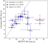 |
Fig. B.1. Comparison between our ROTFIT estimates of RV and values reported by Schneider et al. (2012, red symbols), Donaldson et al. (2016, black symbols), and Gagné et al. (2017, blue symbols), with respective uncertainties. The equality line is traced in gray to guide the eye. |
Some objects in our list have v sin i measurements in Jayawardhana et al. (2006) and Schneider et al. (2012). As illustrated in Fig. B.2 (which excludes TWA 3A for the same reason mentioned above), the three sets of measurements are overall consistent within the estimated uncertainties.
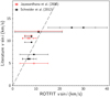 |
Fig. B.2. Comparison between our ROTFIT estimates of v sin i and values reported by Jayawardhana et al. (2006, red symbols) and Schneider et al. (2012, black symbols) for objects in common. Upper limits are marked by arrows. The equality line is traced in gray to guide the eye. |
In Fig. B.3, log g measurements for TWA objects are shown as a function of their Teff. Disk-free TWA objects from Stelzer et al. (2013) are also shown for comparison purposes. The spectra of the latter have been re-analyzed using the latest version of the ROTFIT code, in order to obtain a homogeneous set of atmospheric parameters for disk-bearing and disk-free stars in the association. The log g values adopted here for stars without disk are, therefore, slightly different than those reported in Stelzer et al. (2013) and with smaller associated uncertainties. A list of the newly derived log g parameters for TWA targets in Stelzer et al. (2013) is reported in Table B.1. As discussed in Stelzer et al. (2013), substellar mass objects appear younger on the diagram than earlier-type M-stars stars, although they exhibit a larger vertical scatter and, in some cases, large uncertainties. Objects also appear systematically older than on the HR diagram in Fig. 4, with the bulk of stars at Teff∼3000–4000 K being distributed between the 10 Myr and 20 Myr isochrones according to their log g. This effect, already observed, for instance, in the X-shooter survey of Lupus (see Figs. 4 and 6 of Frasca et al. 2017), is possibly due to issues in the log g vs. age calibration of PMS evolutionary models (see also Herczeg & Hillenbrand 2015).
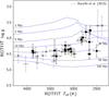 |
Fig. B.3. Measurements of log g for TWA stars with disks (this study, black dots) and without disk (Stelzer et al. 2013, gray diamonds), as a function of their Teff, both derived with ROTFIT. Empty symbols identify objects with disputed membership to the TWA in Gagné et al. (2017). PMS isochrones from Baraffe et al.’s (2015) model grid are overlaid as blue dotted lines for comparison purposes. |
New estimates of the log g parameter for disk-free TWA objects investigated in Stelzer et al. (2013), except TWA 26 and TWA 29.
Appendix C: Classification of Hα line profiles across the TWA sample
The classification of Hα line profiles developed by Reipurth et al. (1996) comprises four morphologically distinct main types: Type I, symmetric; Type II, double-peaked, with the secondary peak being at least half as strong as the primary peak; Type III, double-peaked, with the secondary peak being less than half the strength of the primary peak; and Type IV, which exhibits an absorption feature at the base of the emission line, with no secondary peak. Each of the types II, III, and IV are further distinguished into two subclasses, depending on the location of the secondary peak or absorption feature (blueward or redward of the primary peak). This variety of line profiles reflects contributions from matter inflows and outflows from the inner disk regions, filtered through the geometric configuration of the star-disk system with respect to the line of sight to the observer (e.g., Lima et al. 2010; Kurosawa et al. 2011; Tambovtseva et al. 2014).
In Fig. C.1 we illustrate all Hα line profiles observed for stars in our sample. To test the overall degree of symmetry of the line profiles, we computed how well each of them can be described as a Gaussian8 of equation
![Mathematical equation: $$ \begin{aligned} { y} = a + k \cdot \exp {\left[-\frac{(x - \mu )^2}{2 \sigma ^2}\right]}\,, \end{aligned} $$](/articles/aa/full_html/2019/12/aa35745-19/aa35745-19-eq45.gif) (C.1)
(C.1)
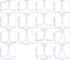 |
Fig. C.1. Hα line profiles for all objects in Table 1, except TWA 3B (which does not exhibit signatures of a disk up to 10 μm) and TWA 40 (for which no line emission was detected). The profiles are sorted according to their qualitative classification following Reipurth et al.’s (1996) scheme: Type I (first and second columns from the left), Type III (first three panels from the top in the third column from the left), Type II/III (last column from the left), Type IV (last panel from the top in the third column). Blue frames are adopted for the Hα profiles of disputed members TWA 22 and TWA 31. Only the Hα profile of the spectrum obtained with lower integration time is shown for TWA 1, because the other spectrum is likely saturated in Hα. When multiple spectra were acquired for the same star at different observing epochs (TWA 27, TWA 30A, TWA 30B), the corresponding Hα profiles are illustrated in separate panels. |
where initial guesses for the free parameters a, k, μ, and σ were defined as the normalized continuum floor (≡1), the normalized peak height, the velocity of the peak, and half the measured full width at half maximum (FWHM), respectively. Strictly speaking, none of the line profiles shown in Fig. C.1 (with the exception of the noisy profile associated with TWA 30B [P287]) can be described satisfactorily9 in terms of a Gaussian curve, according to a χ2 test. However, the best Gaussian fit is sufficient to reproduce the overall Hα profile for objects TWA 3A, TWA 8A, TWA 8B, TWA 22, TWA 30A, and J1247-3816, with point-by-point differences between the observed profile and the fitting curve that are consistent with the ±3 σ noise around the local continuum in the spectrum. These objects exhibit relatively narrow Hα line profiles (FWHM ∼ 70–85 km s−1). TWA 8B, TWA 22, TWA 30A, and J1247-3816 exhibit a single-peak profile with no absorption features, hence falling into the Type I definition of Reipurth et al. (1996). TWA 28 and TWA 32 also exhibit a Type I profile, although diverging from a Gaussian description in the broad wings at velocities ∼100 km s−1. TWA 3A, TWA 8A, and TWA 30B [P287], instead, exhibit a structured peak, with a secondary blueshifted peak appearing above the mean intensity level in the first and the fourth cases; these objects therefore classify as Types II in Reipurth et al.’s scheme. Among the remaining objects, TWA 27 exhibits a secondary redshifted peak or hump, oscillating between Type II and Type III; TWA 1 and TWA 31 exhibit very wide and multi-structured profiles, also oscillating between Type II and Type III; TWA 30B [P087] exhibits an inverse P Cygni profile, therefore qualifying as Type IV.
Appendix D: [O I ] 6300 Å emission measured in the TWA
Table D.1 reports the detected [O I] 6300 Å line luminosities for TWA 1, TWA 30A, TWA 30B, and TWA 31, decomposed into LVC and HVC. The associated uncertainties account for the continuum noise around the line and for the uncertainties on the line profile fit parameters.
[O I] 6300 Å line luminosities measured across our sample, decomposed into LVC and HVC, when detected.
In Fig. D.1 we illustrate the luminosity measured for the [O I] 6300 Å LVC in our sample (TWA 1, TWA 30A, TWA 30B, and TWA 31) as a function of their stellar (L⋆, M⋆) and accretion (Lacc, Ṁacc) parameters. Although the paucity of our sample hampers any detailed considerations with respect to the correlation trends extracted from younger YSO populations, we note that the distribution of points derived here on each panel in Fig. D.1 is globally consistent with earlier results (Nisini et al. 2018; Natta et al. 2014), within the associated dispersions. TWA 30B appears to be an outlier, at least in one epoch, with more intense [O I] 6300 Å LVC than expected, in analogy with Nisini et al.’s (2018) results, based on the estimated Lacc. This is likely due to a severe underestimate of the Lacc of the object, caused by its edge-on configuration and consequent partial concealing of its accretion features. Indeed, as noted earlier, the observed L⋆ would place this source well below the main sequence turnoff on the HR diagram in Fig. 4. Kastner et al. (2016) reported a log L⋆ [L⊙]= − 1.28 for TWA 30B, which indicates that our measurement in Table 2 may be underestimated by three orders of magnitude. The strongest accretors in our sample exhibit Lacc ∼ 0.1 × L⋆, while the bulk of the objects are distributed between Lacc ∼ 0.01 × L⋆ and Lacc ∼ 0.001 × L⋆. Therefore, the actual log Lacc [L⊙] on TWA 30B may be on the order of −3.5, which would project the star within the stripe around the log L([O I] 6300 Å)LVC − log Lacc prescriptions in Fig. D.1. Conversely, the L([O I] 6300 Å)LVC measured for TWA 31 is lower than expected based on the measured Lacc. We note that the detection of [O I] 6300 Å emission for this latter object is somewhat more uncertain than for the other objects, due to a low peak-to-continuum contrast and a noisy line profile, as shown in Fig. 9.
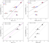 |
Fig. D.1. Logarithmic luminosity of [O I] 6300 Å LVC as a function of log Lacc (upper left panel), log Ṁacc (upper right panel), log L⋆ (lower left panel), and log M⋆ (lower right panel) for stars with detected forbidden line emission in our sample (labeled on each plot). In the upper panels, accretion parameters derived from the Balmer continuum diagnostics (see Sect. 3.1.1) are marked as blue dots, while those derived from the luminosity of emission lines (see Sect. 3.2.1) are marked as red triangles. On each panel, the correlation relationship between the relevant quantities derived by Nisini et al. (2018) is traced as a solid black line, while dotted gray lines mark a range of ±1 dex around the calibration (which corresponds to the vertical spread of points observed on the corresponding diagrams in Nisini et al. 2018). The correlation trends obtained by Natta et al. (2014) are also shown as dashed magenta lines for comparison (left panels). |
Appendix E: Tables of emission line luminosities
Table E.1 lists the measured luminosities of the Balmer series lines from Hα to H15, with relative uncertainties, which were estimated from the rms scatter of the continuum around the position of the line in the spectrum. Table E.2 lists the luminosities of additional lines that were used to estimate  , when detected. Figure E.1 illustrates the FCa II 8542/FCa II 8498 line ratio as a function of Teff for our targets.
Luminosities of Balmer series lines between Hα and H15, when detected.
Luminosities of other emission lines used as tracers of accretion, when detected.
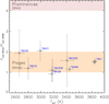 |
Fig. E.1. FCa II 8542/FCa II 8498 ratio measured for TWA targets with detected Ca II IRT emission, as a function of stellar Teff. The range of values typical for solar plages and prominences are marked as a filled strip and a cross-hatched strip, respectively, for comparison purposes. |
Appendix F: Additional figure: Results from the multicomponent fit
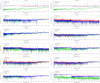 |
Fig. F.1. Results of the multicomponent fit to the observed spectra of our targets (red) around the Balmer jump region. The best-fit photospheric template is illustrated in green, the continuum emission from the hydrogen slab is shown in black, and the total fit is traced in blue. |
All Tables
Mass–dependent values of Ṁacc noise threshold, computed for stars at an age of 10 Myr using the models of Baraffe et al. (2015).
New estimates of the log g parameter for disk-free TWA objects investigated in Stelzer et al. (2013), except TWA 26 and TWA 29.
[O I] 6300 Å line luminosities measured across our sample, decomposed into LVC and HVC, when detected.
Luminosities of other emission lines used as tracers of accretion, when detected.
All Figures
|
Fig. 1. Final processed X-shooter spectrum of TWA 32, separated into UVB (blue), VIS (green), and NIR (red) segments, after correction for telluric features with molecfit and removal of most prominent spikes. The source spectrum after the pipeline reduction but before the telluric correction is shown in black for comparison. |
| In the text | |
|
Fig. 2. Comparison between our L⋆ estimates (see Sect. 3.1.1 and Table 2) and values reported by Ducourant et al. (2014, red symbols) and Kastner et al. (2016, black symbols), corrected for difference in distance between our adopted values and values listed in those references for individual objects. The error bars trace the individual uncertainties associated with the L⋆ values in the compilation of Ducourant et al. (2014), and a typical uncertainty of ±0.2 dex in the other cases, for illustration purposes. The identity line is dashed in gray to guide the eye. |
| In the text | |
|
Fig. 3. Comparison between Teff estimates derived with ROTFIT for all targets and spectra, and Teff values corresponding to estimated SpT for each source (Table 2) using Luhman et al. (2003, red symbols) and Herczeg & Hillenbrand (2014, black symbols) calibrations. The x-axis uncertainties are those derived from the fit; the y-axis uncertainties correspond to half the difference in Teff between consecutive spectral subclasses in the corresponding SpT–Teff scale. The identity line is dashed in gray to guide the eye. |
| In the text | |
|
Fig. 4. HR diagram for stars in Table 2 (black dots) compared with disk–free TWA objects investigated in Manara et al. (2013b) and Stelzer et al. (2013) (gray diamonds), rescaled to Gaia DR2 distances and Herczeg & Hillenbrand’s (2014) SpT–based Teff. Filled symbols identify probable TWA members, open symbols targets with disputed membership. Errors on Teff and log L⋆ are as in Fig. 3 (y-axis) and Fig. 2 (x-axis), respectively. Left panel: theoretical isochrones from different model grids (Baraffe et al. 2015, dotted blue line; Siess et al. 2000, dash-dot red line; Tognelli et al. 2011, dashed green line; Spada et al. 2013, solid black line; Spada et al. 2017, solid yellow line) are shown for comparison on the diagram. The illustrated isochrone ages are, from top to bottom, 1 Myr, 2 Myr, 5 Myr, 20 Myr, and 100 Myr (the isochrones at 1, 2, and 5 Myr are not available from the models of Spada et al. 2013, and the 5 Myr isochrone is not available from the models of Spada et al. 2017). Right panel: mass tracks from the same model grids are illustrated for comparison. Displayed masses are, from right to left: 0.01 M⊙, 0.02 M⊙, 0.05 M⊙, 0.1 M⊙, 0.2 M⊙, 0.4 M⊙, and 0.6 M⊙ (Baraffe et al. 2015); 0.1 M⊙, 0.2 M⊙, 0.4 M⊙, 0.6 M⊙ (Siess et al. 2000; Spada et al. 2013); 0.2 M⊙, 0.4 M⊙, 0.6 M⊙ (Tognelli et al. 2011; Spada et al. 2017). |
| In the text | |
|
Fig. 5. Comparison between log Lacc values measured from excess continuum–fitting with slab emission models (Sect. 3.1.1), and values derived from emission line luminosity (Lline) measurements, using empirical Lline − Lacc calibration relationships from Alcalá et al. (2014). Error bars on the x-axis correspond to a typical uncertainty of 0.25 dex on the Lacc measurements from the multicomponent spectral fit; error bars on the y-axis follow from error propagation including uncertainties on the measured line fluxes, and uncertainties on the calibration relationships, as listed in Alcalá et al. (2014). Green lines connect multiple measurements for the same object. Light dotted lines delimit an area of ±0.3 dex around the equality line (dashed in gray on the diagram). |
| In the text | |
|
Fig. 6. Logarithmic ratio between median Lacc measured from Lline (see text) and stellar L⋆, as a function of Teff. Green vertical lines connect multiple measurements obtained for objects with more than one spectrum. The gray dashed line indicates the emission level below which the impact of chromospheric emission on the observed accretion signatures becomes dominant. |
| In the text | |
|
Fig. 7. Ṁacc vs. M⋆ distribution for stars in our sample, where Ṁacc is calculated from the measured continuum excess luminosity for all objects (filled dots) except TWA 40 and J1247−3816 (empty dots). Smaller red dots mark the locations of TWA 31 (upper point) and TWA 22 (lower point). Green vertical lines connect multiple Ṁacc measurements for the same objects. The shaded gray area traces the estimated chromospheric noise limit for Ṁacc detection, as a function of stellar mass, for stars aged between 3 and 10 Myr on Baraffe et al.’s (2015) isochrone grid. The dash-dot cyan line traces the bimodal Ṁacc − M⋆ relationship derived by Manara et al. (2017a) in the Chamaeleon I star-forming region, with a break at M⋆ ∼ 0.29 M⊙. The solid magenta line traces the bimodal relationship derived in Alcalá et al. (2017) in Lupus, assuming a break at M⋆ = 0.2 M⊙. Double arrows mark the 10th–90th percentile range in Ṁacc covered by the Lupus (magenta) and Chamaeleon I (cyan) populations as a function of mass. The dotted blue line traces a linear fit to the datapoints, which accounts for objects dominated by chromospheric emission (labeled on the diagram) as upper limits. |
| In the text | |
|
Fig. 8. Shapes of Balmer decrements computed for each of our targets (gray lines), defined as logHn/H4 (≡logHn/Hβ). The prototypes of Balmer decrement types identified in Lupus by Antoniucci et al. (2017) are shown with dotted lines for comparison; a thicker stroke is used to emphasize Type 2 (the most common type in their sample and in ours). Typical uncertainties on the log HNup/H4, displayed below the individual Balmer decrement trends, were calculated from the uncertainties associated with the corresponding line flux measurements. |
| In the text | |
|
Fig. 9. Best single-Gaussian (LVC) or double-Gaussian (LVC+HVC) solution obtained for the [O I] 6300 Å line profile decomposition of TWA 1, TWA30 A, TWA 30B, and TWA 31. The LVC is traced with a dotted green line, the blueshifted HVC (when present) is traced as a dotted blue line, and the total fit is traced as a dotted magenta line. |
| In the text | |
|
Fig. 10. Median age and accretion properties normalized to squared mass for six young regions targeted with X-shooter: ρ Ophiuchi (Manara et al. 2015; gray empty triangle), Lupus (Alcalá et al. 2014, 2017; magenta diamond), Chamaeleon I (Manara et al. 2017a; cyan square), σ Orionis (Rigliaco et al. 2012; yellow triangle), TWA (this study; black dot), and η Chamaeleontis (Rugel et al. 2018; green empty square). The horizontal error bars mark the measured age spread among cluster members in the case of ρ Oph, Lupus, and Cha I, and the uncertainty on the nominal age for σ Ori (Bell et al. 2013) and the associations TWA and η Cha (Bell et al. 2015). The vertical errors mark the logarithmic dispersion in |
| In the text | |
|
Fig. 11. Comparison between the Ṁacc − M⋆ distributions obtained from X-shooter data for ρ Ophiuchi, Lupus, Chamaeleon I, σ Orionis, TWA, and η Chamaeleontis (symbols and sources of data as detailed in the caption of Fig. 10). Upper limits in Ṁacc are marked by downward arrows. The horizontal lines mark the median Ṁacc measured in bins of 0.25 dex in log M⋆ for the combined Cha I and Lupus datasets. |
| In the text | |
|
Fig. 12. Logarithmic Ṁacc vs. disk mass distribution for stars in the TWA, compared to the populations of the Lupus and Chamaeleon I star-forming regions. The straight lines mark the Ṁacc − Mdisk relationship predicted for different stellar ages in a scenario of viscous quasi-steady disk evolution (Rosotti et al. 2017). Upper limits are indicated by correspondingly oriented arrows. |
| In the text | |
|
Fig. B.1. Comparison between our ROTFIT estimates of RV and values reported by Schneider et al. (2012, red symbols), Donaldson et al. (2016, black symbols), and Gagné et al. (2017, blue symbols), with respective uncertainties. The equality line is traced in gray to guide the eye. |
| In the text | |
|
Fig. B.2. Comparison between our ROTFIT estimates of v sin i and values reported by Jayawardhana et al. (2006, red symbols) and Schneider et al. (2012, black symbols) for objects in common. Upper limits are marked by arrows. The equality line is traced in gray to guide the eye. |
| In the text | |
|
Fig. B.3. Measurements of log g for TWA stars with disks (this study, black dots) and without disk (Stelzer et al. 2013, gray diamonds), as a function of their Teff, both derived with ROTFIT. Empty symbols identify objects with disputed membership to the TWA in Gagné et al. (2017). PMS isochrones from Baraffe et al.’s (2015) model grid are overlaid as blue dotted lines for comparison purposes. |
| In the text | |
|
Fig. C.1. Hα line profiles for all objects in Table 1, except TWA 3B (which does not exhibit signatures of a disk up to 10 μm) and TWA 40 (for which no line emission was detected). The profiles are sorted according to their qualitative classification following Reipurth et al.’s (1996) scheme: Type I (first and second columns from the left), Type III (first three panels from the top in the third column from the left), Type II/III (last column from the left), Type IV (last panel from the top in the third column). Blue frames are adopted for the Hα profiles of disputed members TWA 22 and TWA 31. Only the Hα profile of the spectrum obtained with lower integration time is shown for TWA 1, because the other spectrum is likely saturated in Hα. When multiple spectra were acquired for the same star at different observing epochs (TWA 27, TWA 30A, TWA 30B), the corresponding Hα profiles are illustrated in separate panels. |
| In the text | |
|
Fig. D.1. Logarithmic luminosity of [O I] 6300 Å LVC as a function of log Lacc (upper left panel), log Ṁacc (upper right panel), log L⋆ (lower left panel), and log M⋆ (lower right panel) for stars with detected forbidden line emission in our sample (labeled on each plot). In the upper panels, accretion parameters derived from the Balmer continuum diagnostics (see Sect. 3.1.1) are marked as blue dots, while those derived from the luminosity of emission lines (see Sect. 3.2.1) are marked as red triangles. On each panel, the correlation relationship between the relevant quantities derived by Nisini et al. (2018) is traced as a solid black line, while dotted gray lines mark a range of ±1 dex around the calibration (which corresponds to the vertical spread of points observed on the corresponding diagrams in Nisini et al. 2018). The correlation trends obtained by Natta et al. (2014) are also shown as dashed magenta lines for comparison (left panels). |
| In the text | |
|
Fig. E.1. FCa II 8542/FCa II 8498 ratio measured for TWA targets with detected Ca II IRT emission, as a function of stellar Teff. The range of values typical for solar plages and prominences are marked as a filled strip and a cross-hatched strip, respectively, for comparison purposes. |
| In the text | |
|
Fig. F.1. Results of the multicomponent fit to the observed spectra of our targets (red) around the Balmer jump region. The best-fit photospheric template is illustrated in green, the continuum emission from the hydrogen slab is shown in black, and the total fit is traced in blue. |
| In the text | |
Current usage metrics show cumulative count of Article Views (full-text article views including HTML views, PDF and ePub downloads, according to the available data) and Abstracts Views on Vision4Press platform.
Data correspond to usage on the plateform after 2015. The current usage metrics is available 48-96 hours after online publication and is updated daily on week days.
Initial download of the metrics may take a while.