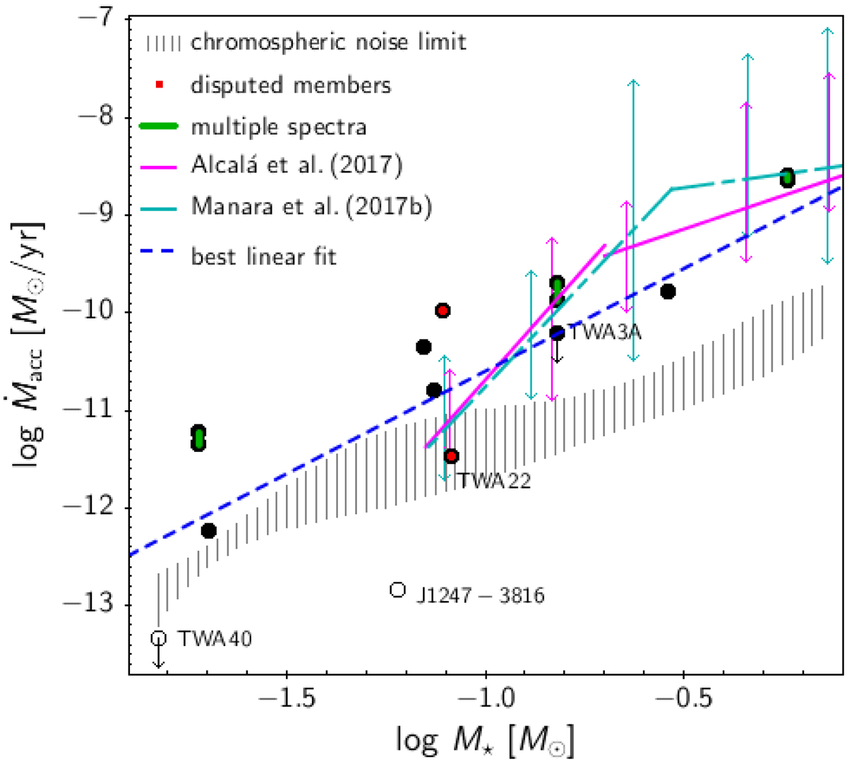
Ṁ_acc vs. M_⋆ distribution for stars in our sample, where Ṁ_acc is calculated from the measured continuum excess luminosity for all objects (filled dots) except TWA 40 and J1247−3816 (empty dots). Smaller red dots mark the locations of TWA 31 (upper point) and TWA 22 (lower point). Green vertical lines connect multiple Ṁ_acc measurements for the same objects. The shaded gray area traces the estimated chromospheric noise limit for Ṁ_acc detection, as a function of stellar mass, for stars aged between 3 and 10 Myr on Baraffe et al.’s (2015) isochrone grid. The dash-dot cyan line traces the bimodal Ṁ_acc − M_⋆ relationship derived by Manara et al. (2017a) in the Chamaeleon I star-forming region, with a break at M_⋆ ∼ 0.29 M_⊙. The solid magenta line traces the bimodal relationship derived in Alcalá et al. (2017) in Lupus, assuming a break at M_⋆ = 0.2 M_⊙. Double arrows mark the 10th–90th percentile range in Ṁ_acc covered by the Lupus (magenta) and Chamaeleon I (cyan) populations as a function of mass. The dotted blue line traces a linear fit to the datapoints, which accounts for objects dominated by chromospheric emission (labeled on the diagram) as upper limits.