| Issue |
A&A
Volume 627, July 2019
|
|
|---|---|---|
| Article Number | A68 | |
| Number of page(s) | 14 | |
| Section | Interstellar and circumstellar matter | |
| DOI | https://doi.org/10.1051/0004-6361/201935506 | |
| Published online | 01 July 2019 | |
IRAS 23385+6053: an embedded massive cluster in the making★
1
INAF, Osservatorio Astrofisico di Arcetri,
Largo E. Fermi 5,
50125
Firenze, Italy
e-mail: This email address is being protected from spambots. You need JavaScript enabled to view it.
2
Max Planck Institute for Astronomy,
Königstuhl 17,
69117
Heidelberg, Germany
3
Max-Planck-Institut für Radioastronomie,
Auf dem Hügel 69,
53121
Bonn, Germany
4
Instituto de Radioastronomía y Astrofísica, Universidad Nacional Autónoma de México,
PO Box 3-72,
58090
Morelia,
Michoacán, México
5
School of Physics and Astronomy, University of Leeds,
Leeds LS2 9JT, UK
6
UK Astronomy Technology Centre, Royal Observatory Edinburgh, Blackford Hill,
Edinburgh,
EH9 3HJ, UK
7
Institute of Astronomy and Astrophysics, University of Tübingen,
Auf der Morgenstelle 10,
72076
Tübingen, Germany
8
INAF, Osservatorio Astronomico di Cagliari,
Via della Scienza 5,
09047
Selargius (CA), Italy
9
Astrophysics Research Institute, Liverpool John Moores University,
Liverpool,
L3 5RF, UK
10
European Southern Observatory,
Karl-Schwarzschild-Str. 2,
85748
Garching bei München, Germany
11
Max-Planck-Institut für Astrophysik,
Karl-Schwarzschild-Str. 1,
85741
Garching, Germany
12
Department of Physics and Astronomy, McMaster University,
1280 Main St. W,
Hamilton,
ON L8S 4M1, Canada
13
I. Physikalisches Institut, Universität zu Köln,
Zülpicher Strasse 77,
50937
Köln, Germany
14
Department of Chemistry, Ludwig Maximilian University,
Butenandtstr. 5-13,
81377
Munich, Germany
15
Centre for Astrophysics and Planetary Science, University of Kent,
Canterbury
CT2 7NH, UK
16
Institut de Radioastronomie Millimétrique (IRAM),
300 rue de la Piscine,
38406
Saint Martin d’Hères, France
17
Center for Astrophysics, Harvard & Smithsonian,
60 Garden Street,
Cambridge,
MA
02138, USA
18
Deutsches SOFIA Institut, Pfaffenwaldring 29, Universität Stuttgart,
70569
Stuttgart, Germany
19
Universidad Autonoma de Chile,
Av. Pedro Valdivia 425,
Santiago de Chile, Chile
Received:
21
March
2019
Accepted:
23
May
2019
Abstract
Context. This study is part of the CORE project, an IRAM/NOEMA large program consisting of observations of the millimeter continuum and molecular line emission towards 20 selected high-mass star-forming regions. The goal of the program is to search for circumstellar accretion disks, study the fragmentation process of molecular clumps, and investigate the chemical composition of the gas in these regions.
Aims. We focus on IRAS 23385+6053, which is believed to be the least-evolved source of the CORE sample. This object is characterized by a compact molecular clump that is IR-dark shortward of 24 μm and is surrounded by a stellar cluster detected in the near-IR. Our aim is to study the structure and velocity field of the clump.
Methods. Observations were performed at ~1.4 mm and employed three configurations of NOEMA and additional single-dish maps, merged with the interferometric data to recover the extended emission. Our correlator setup covered a number of lines from well-known hot core tracers and a few outflow tracers. The angular (~0′′.45–0′′.9) and spectral (0.5 km s−1) resolutions were sufficient to resolve the clump in IRAS 23385+6053 and investigate the existence of large-scale motions due to rotation, infall, or expansion.
Results. We find that the clump splits into six distinct cores when observed at sub-arcsecond resolution. These are identified through their 1.4 mm continuum and molecular line emission. We produce maps of the velocity, line width, and rotational temperature from the methanol and methyl cyanide lines, which allow us to investigate the cores and reveal a velocity and temperature gradient in the most massive core. We also find evidence of a bipolar outflow, possibly powered by a low-mass star.
Conclusions. We present the tentative detection of a circumstellar self-gravitating disk lying in the most massive core and powering a large-scale outflow previously known in the literature. In our scenario, the star powering the flow is responsible for most of the luminosity of IRAS 23385+6053 (~3000 L⊙). The other cores, albeit with masses below the corresponding virial masses, appear to be accreting material from their molecular surroundings and are possibly collapsing or on the verge of collapse. We conclude that we are observing a sample of star-forming cores that is bound to turn into a cluster of massive stars.
Key words: stars: early-type / stars: formation / stars: massive / ISM: individual objects: IRAS 23385+6053
Based on observations carried out with IRAM/NOEMA. IRAM is supported by INSU/CNRS (France), MPG (Germany), and IGN (Spain).
© ESO 2019
1 Introduction
Studies of high-mass (≳104 L⊙) star formation have been hindered until recently by limited angular resolution and sensitivity. Young early-type stars are born deeply embedded in their parental cocoons, which makes observations longward of a few 100 μm necessary toinvestigate the gas and dust emission from their natal environment. In turn, this makes interferometric observations at submillimeter and millimeter wavelengths the only possibility to achieve the sub-arcsecond resolutions needed to study objects typically located at a distance of several kiloparsecs.
The advent of instruments such as the Atacama Large Millimeter/submillimeter Array (ALMA), the NOrthern Exte- nded Millimeter Array (NOEMA), and the upgraded Submillimeter Array (SMA) has allowed a breakthrough in this respect. Not only do the superior angular resolution and sensitivity make it possible to resolve structures at ≲200 au and up to distances of several kiloparsecs, but the large number of antennas allows good sampling of the u, v plane in a short time, enabling surveys of a large number of targets.
With this in mind, we undertook the large program “CORE” (PI Henrik Beuther) with the IRAM interferometer, NOEMA, targeting 20 high-mass star-forming regions. The CORE project has multiple goals: to search for circumstellar disks and study their properties; to establish the level of fragmentation of the parsec-scale molecular clumps harboring the massive young stellar objects (YSOs); and to understand the chemical composition of the gas. While some general results for the whole sample have already been presented in a previous paper (Beuther et al. 2018; hereafter BEU18), in the present study we focus on the particular source IRAS 23385+6053, in the footsteps of other articles of the same sample (Ahmadi et al. 2018; Mottram et al. 2019; Bosco et al. 2019).
IRAS 23385+6053, located at a kinematic distance of 4.9 kpc (Molinari et al. 1998), is also known as Mol160 and was selected as acandidate massive protostar by Palla et al. (1991) on the basis of its IRAS colors. Association with water maser emission (Palla et al. 1991) revealed star formation activity that was later confirmed by other studies such as Molinari et al. (1996), who detected ammonia emission from the source, indicating the presence of dense molecular gas associated with it. Subsequently, Molinari et al. (1998) investigated the structure of the source by comparing interferometric maps of the continuum and molecular line emission with images of the continuum emission in the mid-IR (MIR). From this comparison, one sees that the high-mass object is embedded in an IR-dark core surrounded by an IR-luminousstellar cluster (see Fig. A.26 of Faustini et al. 2009). While the IRAS luminosity of the region is ~ 1.6 × 10⁴ L⊙, MIPSGAL/Spitzer data (Molinari et al. 2008b) have demonstrated that the contribution of the core amounts to only ~ 3 × 10³ L⊙, consistent with IRAS 23385+6053 being a massive protostar in the main accretion phase (Molinari et al 2008a). The rest of the luminosity arises from the surrounding cluster, which is also likely ionizing the two H II regions detected by Molinari et al. (2002). Figure 1a shows a parsec-scale view of the region with the molecular core, the H II regions, and the far-IR (FIR) emission tracing the stellar cluster.
The presence of a compact molecular core was confirmed by the interferometric observations at 3 and 1.3 mm of Fontani et al. (2004) and more recently Wolf-Chase et al. (2012). From their observationsit was also possible to identify a main core and a less prominent, secondary core separated by ~2′′ to the NE. The temperature of the main core was estimated to be quite low (~40 K) compared tothe typical values of hot molecular cores (100–200 K; see Kurtz et al. 2000; Cesaroni 2005) and it was concluded that IRAS 23385+6053 is indeed a rapidly accreting massive YSO in a very early stage of its evolution. Since accretion is tightly connected to ejection, this conclusion appears to have been confirmed by the detection of outflow tracers such as broad line wings and class I methanol maser emission associated with the cores (Molinari et al. 1998; Zhang et al. 2001, 2005; Kurtz et al. 2004; Wolf-Chase et al. 2012), although a clear bipolar outflow pattern (oriented NE–SW) is seen only on large scales (~1.′5) in the single-dish maps of Wu et al. (2005). This orientation is also roughly consistent with the class I CH3 OH masers, which are distributed over a region of 6′′ × 3′′ elongated in the NNE–SSW direction and centered on the molecular core detected by Molinari et al. (1998). In summary, all these characteristics make IRAS 23385+6053 in all likelihood the youngest object of the CORE sample.
In the present study, we make use of the new high-resolution and high-sensitivity NOEMA observations to pursue the investigation of IRAS 23385+6053 and establish its structure on scales of ~0.02 pc. After describing the observations in Sect. 2, we present the results in Sect. 3, while Sect. 4 is devoted to the derivation of the physical parameters of the cores and a detailed analysis of each of them. In Sect. 5 we discuss a possible scenario for IRAS 23385+6053 and compare its properties to those of similar regions. Finally, a summary is given in Sect. 6.
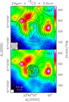 |
Fig. 1 Panel a: map of the emission integrated over the 13CO(2–1) line (solid contours) overlaid on an image of the continuum emission at 24 μm (from Molinari et al. 2008b). The latter has an angular resolution of 6′′. The 13 CO map was obtained with the IRAM 30-m data at a resolution of 12′′ (the beam is shown in the bottom left corner). Solid contour levels range from 20 to 84 in steps of 8 K km s−1. The dotted contours represent a map of the 3.6 cm continuum emission imaged with the VLA Molinari et al. (2002) and range from 0.5 to 2.3 in steps of 0.3 mJy beam−1. The synthesized beam is 10′′.2 × 9′′.0 with PA = −59°. Panel b: same as top panel, where solid contours are a map of the emission averaged over the 13 CO(2–1) line, obtained after merging the NOEMA with the IRAM 30-m data. The resulting synthesized beam is 0′′. 49×0′′.44 with PA = 57° (shown in the bottom left corner). The circle corresponds to the half-power beam width of the NOEMA antennas. The contour levels range from 36 to 144 in steps of 18 mJy beam−1. |
2 Observations
2.1 IRAM/NOEMA interferometer
The region IRAS 23385+6053 was observed in the framework of the NOEMA large program CORE. Details about the program and sample can be found in BEU18. Sources were always observed in pairs of two in the track-sharing mode. In this case, IRAS 23385+6053 was observed together with G108.7575–0.986 in three configurations (A, C and D) between January 2015 and October 2016. The number of antennas in the array varied between 6 and 8. The phase center for IRAS 23385+6053 was α(J2000.0) 23h 40m54. s400 and δ(J2000.0) +61°10′28′′.020 with the velocity of rest of –50.2 km s−1. As gain calibrator, we used the quasar 0059+581, and bandpass and flux calibrators were 3C 454.3 and MWC 349.
The spectral range covered with the broad-band WIDEX correlator was between 217.167 and 220.834 GHz at 1.95 MHz spectral resolution (corresponding to ~2.7 km s−1). Furthermore, eight narrow-band high-spectral-resolution units (~0.5 km s−1) were distributed over the bandpass, mainly covering lines from CH3 CN and H2 CO (for more details see Table 2 in BEU18).
Data calibration and imaging were mainly conducted within the GILDAS framework, with the calibration package CLIC and the imaging program MAPPING. The continuum was produced by collapsing the line-free part of the spectrum into a single continuum channel. Furthermore, the continuum data were self-calibrated in CASA to improve the signal-to-noise ratio (S/N). The continuum 1σ rms of the final images is 0.11 mJy beam−1, and for the line cubes we achieved a typical rms of ~6 mJy beam−1 in a 0.5 km s−1 channel. The spatial resolutions of the continuum and line data are 0′′. 46 and ~0′′.9, respectively, due to the different weighting adopted (uniform for the continuum, robust = 5 for the lines). The absolute flux scale is estimated to be correct to within 20%.
2.2 IRAM/30 m telescope
The above interferometer data were complemented with short spacing observations at the IRAM 30 m telescope. Details of the 30 m observations can be found in Ahmadi et al. (2018) and Mottram et al. (2019). Each source was observed in the 1.4 mm band in the on-the-fly (OTF) observation mode in map sizes of typically 1′ × 1′. On-the-fly maps were conducted in both right ascension and declination directions to reduce scanning effects. Calibration of the single-dish data was done in CLASS, and the merging of the single-dish and interferometer data was again conducted within the MAPPING program. While most compact structures were still cleaned with the CLARK algorithm, the more extended 13 CO(2–1) data were imaged with the Steer-Dewdney-Ito (SDI) method. Details of the merging and imaging are given in Mottram et al. (2019). The resulting angular resolution and 1σ rms in a 3 km s−1 channel are ~0′′.46 and 2 mJy beam−1, respectively.
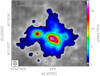 |
Fig. 2 Map of the 1.4 mm continuum emission from IRAS 23385+6053. The values of the contour levels are marked in the color scale to the right. The minimum contour level (0.55 mJy beam−1) corresponds to 5σ. The crosses indicate the positions of the three cores identified by BEU18, corresponding to A1, B, and E in Table 1. |
3 Results
Below we present our main findings. Unless otherwise specified, the maps used in our study are those obtained with the NOEMA interferometer, because only the emission of the CO isotopologs may require merging the NOEMA and 30 m data to be properly imaged.
3.1 Continuum emission
A study of the continuum emission from IRAS 23385+6053 and the other sources of the CORE sample has already been presented by BEU18. Using the CLUMPFIND algorithm, they identified three cores, whose total flux density is ~180 mJy. This is greater than the value of ~150 mJy obtained by Fontani et al. (2004). Such a difference is larger than the noise of the map of Fontani et al. (2004) (~2 mJy beam−1) and could be due to the different u, v coverage of the two data sets. In fact at the time of the Fontani et al. (2004) observations the Plateau de Bure interferometer was equipped with only five antennas, and two configurations of the array were used, compared with our NOEMA observations performed with a number of antennas ranging from six to eight and three different configurations. In particular, unlike Fontani et al. (2004), we also used the most compact (D-array) configuration and it is therefore not surprising that part of the flux density present in our images is filtered out in their data. Figure 2 shows the map of the continuum emission, with the positions of the three cores identified by BEU18 overlaid.
3.2 Line emission
While the correlator setup covers many potentially useful molecular lines, only some of these have been detected with a typical 1σ noise of 3 mJy beam−1 (~0.1 K) in a 3 km s−1 channel. The most prominent are the 13CO and C18 O(2–1) transitions. However, these CO isotopologs are largely sensitive to extended emission, which masks the compact emission from the core. In Fig. 1 we compare a map of the mean emission in the 13 CO(2–1) line to the Spitzer/MIPS image of the regionat 24 μm. More precisely, in Fig. 1a we show the 13CO map made with the 30 m telescope, while in Fig. 1b the same map has been obtained after merging the 30 m and NOEMA data. One can see that the compact core is embedded in a larger emitting region extending over at least ~20′′ (0.48 pc). As noted by Molinari et al. (2008b), the core is detected at 24 μm (whereas it is IR-dark at shorter wavelengths). It is worth noting that no clear bipolar outflow structure can be identified from our CO data, either in the channel maps or in the spectra. Although this might be due to the limited spectral resolution (3 km s−1) and the relatively small region covered by the observations, one must also consider that 12 CO would be a better outflow tracer than its isotopologs, and the outflow orientation could also prevent its detection if the axis lies close to the plane of the sky and/or the gas is ejected at low velocity. The 13 CO emitting region appears to lie between the two compact H II regions (dotted contours in Fig. 1) imaged at 3.6 cm by Molinari et al. (2002), which are ionized by B-type stars belonging to the surrounding cluster.
The present study is focused on compact cores. These are much more easily traced by other molecular species than the CO isotopologs. Our correlator setup covers several transitions of different molecular species, as one can see in the broadbandspectrum shown in Fig. 3, obtained with the WIDEX correlator towards the peak of the emission. However, for our purposes we focus mostly on the lines also covered by the high-spectral-resolution (0.5 km s−1) units of the narrow-band correlator and marked in red in Fig. 3. These belong to formaldehyde (H2 CO), methanol (CH3 OH), methyl cyanide (CH3 CN), cyanoacetylene (HC3 N), carbonyl sulfide (OCS), and ketene (H2CCO). The maps of the emission averaged over the lines of these species are shown in Fig. 4. Visual inspection of both these images and the continuum emission map in Fig. 2 allows us to identify six cores, whose positions are marked in Fig. 4 with crosses.
More specifically, cores A1+A2, B, and E were found by BEU18 from the continuum map and are clearly seen in the CH3 OH map in Fig. 4, while core D is well defined in the CH3 OH map, and core C appears as a separate entity only in the H2CCO map. We point out that we decided to split core 1 in Table A.1 of BEU18 into two cores, A1 and A2, because the head-tail structure seen in the continuum is not reproduced in some of the lines. In particular, the HC3 N, OCS, and CH3 CN emission seems to trace a circular, barely resolved core located at the position of the continuum peak (A1).
Not all molecules are detected in all cores. Table 1 lists the tracers revealed in each core, while Fig. 5 illustrates the locations of the cores through a sketch to facilitate core identification and comparison with the maps.
An interesting feature that can be seen in the maps of the H2 CO and CH3 OH emission is the presence of two blobs, F1 and F2 (see Fig. 6), separated by ~10′′ or 0.24 pc and symmetrically disposed to the SE and NW of core C. This is shown in Fig. 6, where the dashed line joins the two blobs. While these might be two additional cores, the nondetection of continuum emission from them hints at a different nature. We propose that they could be the tips of the lobes of a bipolar outflow originating from C or a nearby, low-mass undetected core. Indeed, the sensitivity (at a 5σ level) of our continuum map is ~0.1–0.5 M⊙ for a dust temperature in the range 20–70 K. These values are typically above the mass of envelopes or disks around class I YSOs. We discuss this outflow hypothesis further in Sect. 4, whereas in Sect. 4.2 we comment on the possible existence of another outflow powered by a YSO in core A1.
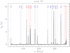 |
Fig. 3 Spectrum obtained with the WIDEX correlator at low spectral resolution towards the peak of core A1. Only the strongest molecular transitions are indicated. The red color denotes the lines observed also at high spectral resolution. |
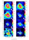 |
Fig. 4 Maps of the mean emission in various molecular lines. For the sake of direct comparison with the line maps we show again the map of the continuum emission in the bottom right panel. For each map, the values of the contour levels are marked in the corresponding color scale. The crosses and letters indicate the positions of the six cores identified by us (see also Fig. 5). Cores A1, B, and E correspond to the crosses in Fig. 2. The ellipse in the bottom right of each panel is the synthesized beam. |
 |
Fig. 5 Sketch of the cores identified by us in IRAS 23385+6053. The contour corresponds to the 5σ level of the continuum emission. The two arrows and arcs indicate the direction and location of the expanding lobes (F1 and F2) of the bipolar outflow detected in the H2 CO and CH3 OH emission, perhaps originating from core C. |
List of tracers detected in each core and corresponding parameters.
4 Analysis
The goal of our study is to establish the nature of the cores identified in our maps. In the following we derive the core physical parameters and analyze each of them in more detail.
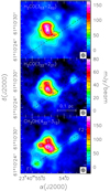 |
Fig. 6 Same as Fig. 4 but over a larger region and only for the H2 CO and CH3 OH lines. The dashed line denotes the direction defined by the two emission blobs, F1 and F2, located to the SE and NW of the main cores, respectively. |
4.1 Physical parameters of the cores
The observed ratio between the brightness temperatures of the H2 CO (322–221) and (303 –202) transitions over the cores is in all cases >0.56, the maximum local thermodynamic equilibrium (LTE) ratio expected in the optically thin case1. This indicates that the lines must be optically thick and their ratio cannot be used to estimate the gas temperature and column density of the cores. For the same reason, H2CO is not suitable for the study of the velocity field, because it traces the envelope around the cores as suggested by the size of the H2 CO emission in Fig. 4. From this figure, one sees that most of the cores are recognizable in the methanol map and we therefore prefer to use this species to obtain a picture of the core physical properties. In Fig. 7 we show maps of the line velocity and full width at half maximum obtained from the first and second moments of the CH3OH line. Overlaid on this is the map of the zero moment (integrated intensity) in the same line.
As one can see from Fig. 3, two more lines of methanol are detected in the bandwidth covered by the WIDEX correlator: the 80 –71 E2 and 201 –200 E1 transitions. One can use these transitions to calculate the rotational temperature, Trot, of the CH3OH gas all over the cores. For this purpose we used the eXtended CASA Line Analysis Software Suite (XCLASS) tool2 (Möller et al. 2017), which simultaneously fits the lines of a molecular species assuming LTE by varying the relevant physical parameters, namely the source angular size, rotational temperature, column density of the molecule, systemic local standard of rest (LSR) velocity, and line width. One of the advantages with respect to rotation diagrams is that XCLASS takes into account the line opacities in the fit. In our case, the region over which CH3OH is detected is much greater than the synthesized beam and we therefore assume a beam filling factor equal to 1. The maps of Trot and CH3OH column density are shown in Fig. 8, where both quantities peak towards the position of A1.
The same method can be applied to the CH3CN(12–11) K = 0–6 transitions, which are known to be excellent hot core tracers. As such, these are well suited to estimating the physical parameters of chemically rich cores like A1 and A2 and indeed the CH3CN emission is detected only towards these two cores. We present the corresponding Trot and column density maps in Fig. 9. The obvious difference with respect to Fig. 8 is that the temperature obtained from CH3CN is about twice as high as that derived from CH3OH. While this could be due to methanol being sub-thermally excited (Bachiller et al. 1995; Kalenskii & Kurtz 2016), it is most likely that the interplay between opacity and temperature gradients plays a dominant role. Unlike the other cores, A1 coincides with the peak of column density and it is therefore possible that species with different abundances (and opacities) trace regions with different temperatures.
Now we compute the mean values of the physical parameters of the cores. For this purpose, it is necessary to establish the border of each core. In order to simplify the problem, we assume the cores to be spherical, so that all we need to estimate is the core radius. In Table 2 we give the peak positions of the cores determined from the line and continuum maps. In particular, the positions of cores A1, B, and E are taken from Table A.1 of BEU18. These authors used CLUMPFIND to determine the core sizes, but this method was applied to the continuum image where only three cores were identified. Here we prefer to use a different approach. For each core, we consider the separation from the nearest of the other cores and assume that this is twice the radius of the core. We give the radii, Rc, in Table 2. These values should be considered with two caveats in mind. On the one hand, the method used by us overestimates the radius, because two neighboring cores are not necessarily in contact. On the other hand, we underestimate the separation because we see only the projection of it on the plane of the sky.
We calculate the mean values of the LSR velocity (V LSR), line full width at half maximum (ΔV), and temperature (Trot) by averaging the corresponding CH3OH parameters (see Figs. 7 and 8) over the surface of each core. Finally, we obtain the total core flux densities (Sν) by integrating the continuum emission (Fig. 2) inside the borders of the cores. All these quantities are listed in Table 2, where we also give virial masses, Mvir, and the core masses,  computed from the temperature, line widths, and flux densities according to Eq. (3) of MacLaren et al. (1988) and Eq. (1) of Schuller et al. 2009, under the assumptions of constant density, gas-to-dust mass ratio of 150, and dust opacity of 0.9 cm2 g−1 at 1.4 mm. In the same table we report the H2 densities, for a mean molecular weight of 2.8, and the ratios
  .
.
Clearly, the velocity changes significantly from core to core, with cores A1, A2, and E being redshifted by at least ~1 km s−1 with respect to B and D, while cores A1 and D are those with the largest line widths and possibly the highest level of turbulence. We note that in all cases the line is wider than expected from pure thermal broadening (<0.42 km s−1 for T < 120 K – see Fig. 9), which implies a contribution from nonthermal motions. The line width is also large close to core C (see Fig. 7b), where a blueshifted “spot” is seen in the velocity map (Fig. 7a; see also Sect. 4.5). Whether or not core C is really associated with such a feature is questionable. We remind the reader that this core has been identified only from the faint H2 CCO emission, which makes it difficult to determine a precise position for it. In any case, it appears that close to the geometrical center of the (putative) outflow there is a small region with a large velocity dispersion, which could contain the source powering the flow. An alternative possibility is that this “spot” is where the flow from C impinges on the dense gas, thus causing the observed enhancement of the line width. It is worth noting that Wolf-Chase et al. (2012) detected an H2 knot (MHO 2921 in their notation) close to core C, which is probably due to emission from shocks.
The velocity difference between blobs F1 and F2 is small, only ~1 km s−1, but this is expected if the outflow lobes lie close to the plane of the sky. However, very little velocity dispersion (the line FWHM is ~2 km s−1) is observed towards these blobs, in contrast with the expected line broadening at the tips of a bipolar flow. We discuss the outflow hypothesis further in Sect. 4.5.
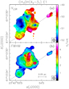 |
Fig. 7 Panel a: map of the zero moment (integrated intensity; contours) of the CH3 OH(42–31) E1 line overlaid on the map (color image) of the first moment of the same transition. Contour levels range from 0.05 to 1.25 in steps of 0.2 Jy beam−1 km s−1. The ellipse in the bottom right represents the synthesized beam. The dashed line has the same meaning as in Fig. 6. Panel b: same as top panel, but for the second moment of the methanol line. |
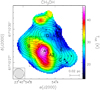 |
Fig. 8 Maps of the CH3OH rotational temperature (color image) and column density (contours) obtained with the XCLASS program. The labels indicate the cores. Contour levels range from 2 × 10¹⁵ to 1.1 × 10¹⁶ in steps of 1015 cm−2. Typical uncertainties on the values of the rotational temperature are 10–20%. The ellipse in the bottom left denotes the synthesized beam. The dashed box corresponds to the region shown in Fig. 9. |
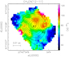 |
Fig. 9 Maps of the CH3CN rotational temperature (color image) and column density (contours) obtained with the XCLASS program. The labels have the same meaning as in Fig. 4. Contour levels range from 2 × 10¹³ to 1014 in steps of 1013 cm−2. Typical uncertainties on the values of the rotational temperature are 10–20%. |
4.2 Core A1
As already explained, we prefer to identify two cores (A1 and A2) where the analysis of BEU18 finds only one. This choice, based on the morphology of the line emission, is further supported by the different kinematical properties recognizable in Fig. 7, especially for the line FWHM which is larger (by ~1 km s−1) in A1 compared to A2.
The velocity field in A1 can be better analyzed by means of high-density, high-temperature tracers such as CH3CN. In Fig. 10 we show a map of the peak velocity of the CH3CN(12–11) transition obtained by fitting Gaussian profiles simultaneously to the strongest (K = 0–4) components, after fixing the line separations to the laboratory values and forcing the line widths to be identical. This method has the advantage of reducing the velocity and line width uncertainties with respect to fitting each K component independently or computing the first and second moments of the lines. The velocity pattern presents two redshifted and two blueshifted peaks defining two velocity gradients along directions (see the dotted and dashed lines in Fig. 10) roughly perpendicular to each other. The CH3CN emission (see contour map in Fig. 10) clearly peaks towards A1, which proves that this emission is largely dominated by A1 and the CH3CN velocity is affected only marginally by the gas in A2. In the following, we discuss three scenarios that could explain the observed velocity field in core A1.
4.2.1 Keplerian disk with expansion
The presence of two velocity gradients, directed SE–NW and SW–NE, could be due to the combination of Keplerian rotation and expansion along the surface of the disk, a situation reminiscent of disk winds.
It is worth noting that we cannot distinguish between expansion and infall on the basis of the observed velocity pattern, since in both cases the projected velocities along the line of sight give origin to the same type of velocity field. In practice, reversing the sign of the radial velocity from positive (for expansion) to negative (for infall) only swaps the red- and blueshifted sides of the disk, which can be compensated with a rotation by 180° of the position angle of the disk. Here, we rule out infall a priori, because the existence of a pair of blue- and redshifted velocity peaks close to the disk border can be explained only if the radial velocity component increases with radius. This situation is in contrast with infall, which accelerates towards the star, whereas it is acceptable for expansion, where the material is accelerated outward.
While a physical model to reproduce the observed velocity and intensity goes beyond the scope of the present article, we can compare thevelocity map in Fig. 10 with the map of the line-of-sight velocity computed from a purely kinematical model assuming Keplerian rotation and radial expansion in a geometrically thin disk. The observed velocity is given by the expression
 (1)
(1)
where x and y are Cartesian coordinates in the plane of the sky with y along the projected major axis of the disk, V sys is the systemic velocity with respect to the local standard of rest (LSR),  , Ro is the outer radius of the disk, vrot and vrad are the azimuthal and radial velocity components in the plane of the disk at Ro, θ is the anglebetween the disk axis and the line of sight, and we have assumed α = −1∕2 for Keplerian rotation and β = 1 for expansion. In Fig. 11 we show the velocity map obtained for fiducial values of the parameters (θ = 30°, vrot = 0.7 km s−1, vrad = 2 km s−1, V sys = −50.7 km s−1), obtained by visual comparison with Fig. 10. In particular, the inclination θ was obtained from the ratio between the minor axis (~2′′) and the major axis (~2′′.3) of the velocity map in Fig. 10, as θ = arccos(2∕2.3). We note that all lengths are normalized with respect to Ro and the velocity is computed down to a minimum radius Ri = 0.15 Ro.
The model presents a number of features which are clearly not in agreement with the data. For example, the two inner velocity peaks are too close to the center of the disk and the directions of the two velocity gradients (dashed and dotted lines in Fig. 11) are not perpendicular to each other as they are in Fig. 10. However, we stress that the comparison between Figs. 10 and 11 is only qualitative, as our calculations do not take into account the angular resolution of the observations and no attempt is made to compute the line intensity and width. We do not want to fit the data but only to show that rotation plus expansion could mimic the existence of two pairs of blue- and redshifted velocity peaks (connected by the dotted and dashed lines in Fig. 11), one located inside the disk, the other close to the border of it. These double peaks generate the twist in the velocity pattern that is seen in the data.
Since inthis model the disk is undergoing Keplerian rotation, one can compute the stellar mass from the high-velocity peaks close to the center of the disk. From Fig. 10 one obtains a rotation velocity3 of 0.5 km s−1 at a radius of 0′′. 73 (or 3600 au), which implies a dynamical mass Mdyn ~ 1 M⊙. This value appears far too small, compared to the mass of the core (~24 M⊙; see Table 2), to satisfy the condition Mstar > Mdisk for Keplerian rotation. Moreover, it is very unlikely that a solar-type star associated with a chemically rich molecular core (“hot corino”) could be detected at a distance of 4.9 kpc. Finally, the luminosity of the source (3000 L⊙) is three orders of magnitude greater than that of a solar-type star.
Most of these problems can be solved if the disk is sufficiently inclined with respect to the line of sight. A stellar luminosity of 3000 L⊙ corresponds to a stellar mass of M* ≃ 9 M⊙ (Mottram et al. 2011), which in turn implies an inclination of  . An even smaller θ is needed to justify M* > 24 M⊙. While an almost face-on disk is consistent with the findings of Molinari et al. (1998), the SE–NW orientation of the disk (and associated outflow) axis is not. In fact, the maps in Fig. 4 of Molinari et al. (1998), as well as the large-scale maps of Wu et al. (2005), suggest that the SiO flow is oriented NE–SW. In addition, the luminosity of a >24 M⊙ star should exceed the observed luminosity of 3000 L⊙. We therefore believe that the model consisting of a Keplerian disk with expansion is not acceptable.
Parameters of the cores in the IRAS 23385+6053 region.
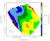 |
Fig. 10 Map of the CH3CN(12–11) line emissionaveraged over the K = 0 and 1 components (contours) overlaid on the map of the velocity in the same line, obtained by simultaneously fitting the K = 0–4 components as explained in the text. Labels A1 and A2 mark the center positions of the corresponding cores. Contour levels range from 9.5 (5σ) to 57 in steps of 9.5 mJy beam−1. The dotted and dashed LINES indicate the approximate directions of the two velocity gradients. |
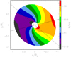 |
Fig. 11 Model velocity map for a geometrically thin disk undergoing both Keplerian rotation and expansion with radial velocity proportional to the radius. Fiducial values have been assumed for the parameters (see text). The map has been rotated by 45° to ease the comparison with Fig. 10. The dotted and dashed lines indicate the directions of the two velocity gradients defined by the blue- and redshifted velocity peaks. |
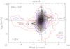 |
Fig. 12 Line intensity as a function of velocity and position along the dashed line in Fig. 10 (position angle −56°). Different colors correspond to different molecular species as indicated in the bottom right. The cross in the bottom left gives the velocity and angular resolution. The arrows indicate the possible “spurs” typical of the pattern corresponding to Keplerian rotation. The yellow butterfly-shaped curve is the region inside which emission is expected for a Keplerian disk rotating about an 8 M⊙ star. Contour levels range from 15 (5σ) to 123 in steps of 18 mJy beam−1 for OCS, from 17.5 (5σ) to 332.5 in steps of 52.5 mJy beam−1 for CH3 OH, and from 13.2 (4σ) to 151.8 in steps of 19.8 mJy beam−1 for HC3 N. |
4.2.2 Rotating disk
An alternative scenario is that the velocity pattern in Fig. 10 is due to the combination of a rotating disk oriented SE–NW and a bipolar outflow in the NE–SW direction. The SE–NW velocity gradient can be investigated through the position–velocity (PV) diagram along a suitable cut (dashed line in Fig. 10). Figure 12 shows this diagram for the lines of three species and in all cases the plot is vaguely reminiscent of the typical “butterfly-shaped” pattern consistent with Keplerian rotation (see the yellow curves in the figure; e.g., Cesaroni et al. 2005).
Under the assumption of Keplerian rotation, the velocity and position of the two putative “spurs” indicated in Fig. 12 can be used to estimate a dynamical mass, which for a Keplerian disk is the mass of the central object. We stress that we basically use the same approach as in Sect. 4.2.1 to derive an estimate of the stellar mass, with the only difference being that here the disk is oriented SE–NW (and hence responsible for the corresponding velocity gradient), whereas in Sect. 4.2.1 it is oriented NE–SW.
For a rotation velocity of ~1 km s−1 at a radius of ~1′′.5 or 0.036 pc, one obtains a stellar mass of ~8 M⊙ (see the Keplerian pattern in Fig. 12). Although this value is in good agreement with the core luminosity of 3000 L⊙ estimated by Molinariet al. (2008b), it is small compared to the mass of the core (24 M⊙), inconsistent with the assumption of Keplerian rotation, which requires the gas mass to be negligible with respect to the stellar mass. This problem can be solved if the disk is sufficiently inclined. Since M* = 8M⊙∕sin2θ (with θ angle between the disk axis and the line of sight), the stellar mass can exceed 24 M⊙ for θ < 35°. However, the luminosity of a >24 M⊙ star is > 7 × 10⁴ L⊙ (Mottram et al. 2011), much greater than the estimated value of 3000 L⊙.
All the above assumes that the disk is Keplerian. If one drops this assumption and considers a self-gravitating disk, the dynamical mass estimated above (8 M⊙) corresponds to the mass of the disk. As shown above, for a suitable inclination this can match the mass of 24 M⊙ obtained from the millimeter continuum. Since the disk is self-gravitating, the stellar mass must be significantly less than the disk mass, consistent with ~9 M⊙ derived from the luminosity of 3000 M⊙. In fact, a self-gravitating disk oriented close to face-on is in agreement with the findings of Molinari et al. (1998). Also, the size appears more consistent with those of “toroids” than with the typical diameters (~1000 au) of accretion disks around B-type stars (see Beltrán & de Wit 2016). Finally, a butterfly-shaped PV diagram is not in contradiction with a self-gravitating disk because its rotation curve could mimic that of a Keplerian disk (e.g., Bertin & Lodato 1999; Douglas et al. 2013; Ilee et al. 2018). It is worth stressing that the uncertainties on the estimate of the dynamical mass are large. For example, assuming a radius of 2′′ and a corresponding rotation velocity of 1.5 km s−1, one obtains 25 M⊙. The core mass is also uncertain, as it is inversely proportional to the dust absorption coefficient (assumed 0.9 cm2 g−1 by BEU18), which might be underestimated by a factor of approximately two (see Table 1 of Ossenkopf & Henning 1994). Furthermore, the gas-to-dust mass ratio could be 100 instead of 150 (assumed by BEU18 in their calculations), which may cause an overestimate of the mass by a factor 1.5.
Despite all these caveats, we believe that the hypothesis of a self-gravitating disk oriented SE–NW and rotating about a ~9 M⊙ star is plausible. We note that in this case, the NE–SW orientation of the disk axis would be consistent with that of the large-scale flow imaged by Wu et al. (2005).
4.2.3 Bipolar outflow
A third possibility to explain the observed velocity gradient is that of a compact bipolar outflow. Evidence for an outflow was also provided by Molinari et al. (1998) in terms of broad wings of the HCO+(1–0) and SiO(2–1) lines. Since no clear bipolar structure was identified, these authors proposed that the outflow is directed close to the line of sight. This is at odds with the small velocity difference (~1 km s−1) between thered- and the blueshifted emission observed by us, because typical flow speeds are much greater (>10 km s−1) and projection effects should not matter if the flow is directed close to the line of sight. If an outflow is traced by the SiO emission, we believe that it should be very compact and with a significant inclination with respect to the line of sight.
To helpdistinguish between the disk and outflow scenarios we consider Fig. 9. Interestingly, the temperature rises from the center to the border of the core along the direction of the SE–NW velocity gradient, while the reverse occurs for the column density. This behavior seems more compatible with a bipolar outflow than a rotating disk, because in the latter the temperature is expected to decrease with increasing radius. As a matter of fact, it would not be surprising if CH3CN was tracing an outflow, as several studies have detected CH3CN in outflows as well (e.g., Leurini et al. 2011; Busquet et al. 2014; Palau et al. 2017).
We can derive the parameters of the outflow, assuming that all the material traced by the CH3CN line participates in the expansion. As a first step, we estimate the abundance of CH3CN,  , from the ratio between the total number of CH3CN molecules and the total number of H2 molecules. The latter is obtained from the mass of 24 M⊙ from Table 2, while the former can be computed by integrating the CH3CN column density over the map in Fig. 9. We obtain
  , an order of magnitude less than the typical value of hot molecular cores, but plausible for an object in an earlier evolutionary phase (see Gerner et al. 2014). We then calculate the momentum of the flow from the expression
 (2)
(2)
where i is the inclination angle of the outflow axis with respect to the line of sight, the sum is extended over all the pixels of the map in Fig. 9, Ni and V i are the CH3CN column density and velocity at pixel j, V sys the systemic velocity (~ –50.7 km s−1), μ = 2.8 the mean molecular weight, mH the mass of the hydrogen atom, d the distance (4.9 kpc), and δΩ the solid angle of the pixel. We obtain P cosi ≃ 9 M⊙ km s−1. The corresponding timescale of the flow, tout, is given by the ratio between the SE–NW size of the region mapped in Fig. 9 and the maximum velocity range observed over the same region: tout tani = 1′′.9∕1.8 km s−1 = 0.045 pc∕1.8 km s−1 = 2.4 × 10⁴ yr. From this one obtains the momentum rate Ṗ cos2i∕sin i = 3.7 × 10⁻⁴ M⊙ km s−1 yr−1. Assuming momentum conservation in the flow, this value should be valid for the whole outflow, despite the fact that our estimate is obtained for the small region traced by the CH3CN emission.
Taken at face value and using the relationship between Ṗ and luminosity determined by Maud et al. (2015) for a distance-limited sample of outflows from massive YSOs (Log10[Ṗ] = −4.8 + 0.61 Log10[L]), the momentum rate implies a YSO luminosity of ~175 L⊙, far less than the estimate of 3 × 10³ L⊙ obtained by Molinariet al. (2008b), which instead corresponds to Ṗ = 2.1 × 10⁻³ M⊙ km s−1 yr−1. To match this value, the outflow inclination must be i ≃ 70°. Such a largeangle cannot be ruled out a priori, but is inconsistent with the claim of Molinari et al. (1996) that the outflow axis lies close to the line of sight. Moreover, the SE–NW orientation of the putative outflow in the plane of thesky is roughly perpendicular to that of the bipolar flow imaged by Wu et al. (2005) in the 12 CO(1–0) line on the arcmin scale. While comparison between scales that differ by more than an order of magnitude must be taken with caution, we believe that the outflow interpretation for the observed CH3CN velocity field is probably the least likely of all those previously discussed by us.
Based on all the above, we conclude that the CH3CN emission in A1 is unlikely to trace an outflow and we are thus inclined to prefer the disk scenario. It is also possible that the observed velocity field is contributed by an accretion flow (through the disk), as suggested by the redshifted self-absorption seen in the line profiles, as discussed later in Sect. 5.1.
4.3 Core A2
Figures 7 and 10 show that the LSR velocity increases slightly from A1 to A2. Figure 7 also shows that the velocity dispersion is significantly larger in A1 than in A2, while Figs. 4 and 6 demonstrate that the emission in all lines observed by us, as well as in the continuum, is weaker in A2. All of this evidence supports our choice to distinguish this core from A1.
Another important feature denoting a difference between the two cores is the chemical richness. From Table 1, one sees that while all listed species are detected in A1, only two of them are clearly revealed in A2. Finally, Fig. 9 demonstrates that both column density and temperature decrease going from A1 to A2, while the latter is half as massive as the former.
In conclusion, it seems unlikely that A2 is a starless core, given the relatively large temperature (typically ~60 K) obtained from CH3CN. However, the lower mass and turbulence suggest that any YSO in A2 could be less massive and/or in an earlier evolutionary phase than in A1.
4.4 Core B
This core is clearly separated from A1 only in the continuum and CH3OH emission. Although B is a fainter emitter in most tracers with respect to A1 and A2, the mass and temperature are comparable to those of A1 and A2, hinting at a substantial similarity between these cores. The most striking feature of B is the ratio  , which is the only one above unity. We comment on this fact in more detail in Sect. 5.1, but we can already draw the conclusion that B must be virialized or on the edge of collapse, and in all likelihood this core is bound to evolve into a status analogous to that of A1 and A2. Indeed, the lack of emission in most of the observed lines (see Table 1) appears consistent with the idea that this core is in an early evolutionary phase.
4.5 Core C
The most interesting feature of core C is its possible association with the bipolar outflow described in Sect. 3.2. In Fig. 13 we show the PV diagram of the emission along the dashed line in Fig. 6, in three different lines. Several comments are in order for this plot. First of all, there is a velocity trend, outlined by the dashed line in the figure. It is furthermore worth noting that the H2 CCO emission tracing coreC is centrally located with respect to the SE and NW lobes (detected in CH3OH and H2 CO) not only in space but also in velocity. Finally, the CH3OH and H2 CO emission at the center is highly asymmetric in velocity, with a broad blue wing, evident also from the spectrum in Fig. 14. At the sametime, the lack of an equally broad red wing could be explained by the presence of redshifted self-absorption in a core undergoing infall. This is consistent with the blueshifted “spot” visible in Fig. 7a, an indication of infall (see e.g., Mayen-Gijon et al. 2014). These facts suggest that indeed the YSO powering the flow could be embedded in an infalling core characterized by large velocity dispersion. Whether or not this core is indeed core C (i.e., the one identified through the H2 CCO emission) is unclear, as the latter is slightly offset from both the outflow axis (see Fig. 6) and the blueshifted “spot”. In any case, we believe that this outflow cannot be associated with a very massive object, due to the weakness of the line emission from the lobes and the lack of a well-defined core or a YSO powering it.
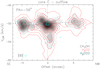 |
Fig. 13 Line intensity as a function of velocity and position along the dashed line in Fig. 6 (position angle –56°). Different colors correspond to different molecular species as indicated in the bottom right. The cross in the bottom left gives the velocity and angular resolution. The dotted vertical line marks the position of core C, while the dashed line outlines the velocity trend observed in the H2 CO and CH3 OH lines. Contour levels range from 15 (5σ) to 225 in steps of 30 mJy beam−1 for CH3 OH, from 18 (5σ) to 338 in steps of 40 mJy beam−1 for H2 CO, and from 16 (4σ) to 32 in steps of 3 mJy beam−1 for H2 CCO. |
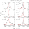 |
Fig. 14 Spectra of the H2CO(303–202) (black solid histogram) and CH3OH(42–31) E1 (red dashed histogram) lines towards the positions of the six cores identified in IRAS 23385+6053. The vertical dotted line is shown to ease the comparison between spectra of different cores. |
4.6 Cores D and E
As one can see in Fig. 4, core D is only well defined in the CH3OH map, while other tracers present at most a tail of emission towards it. Similar to core D, core E is also clearly identified inonly one tracer, this time the continuum emission. In summary, both cores have small masses and are recognizable as such only in one tracer. However, there is an important difference between the two: thevelocity dispersion in D is much greater than that in E, as evidenced by the FWHM of the CH3OH line, which is 1.8 times larger in D than in E (see Table 2). We note that the line of FWHM in D (3.6 km s−1) is even greater than that in A1 (3.2 km s−1), where various signposts indicate star formation activity.
5 Discussion
5.1 A cluster of massive stars in the making?
Based on the analysis presented above, we consider the possibility that IRAS 23385+6053 consists of multiple star-forming cores in an early stage of their evolution. Molinari et al. (2008b) provided evidence that this object is indeed in a protostellar phase, prior to the formation of an H II region. However, their analysis assumes the presence of a single YSO, which we associate with A1, because this core seems to be the most active in terms of star formation and is hence likely to dominate the luminosity and mass estimates used by Molinari et al. (2008b) to establish the evolutionary phase of IRAS 23385+6053.
We have shown that A1 is surrounded by other cores, most of which could contain embedded YSOs undergoing accretion. The first question we are asking is whether core formation proceeded through thermal Jeans fragmentation. This can be elucidated by comparing the Jeans length of the overall region with the mean separation of the cores. The latter is Δ ≃ 1′′.2 = 5900 au, whereas the former can be computed from  , assuming the mean temperature (T ≃ 30 K) from CH3OH and deriving the gas density (
 cm−3) from the ratio between the total core mass (~70 M⊙, see Table 2) and the volume occupied by the cores. The diameter of this volume (assuming spherical symmetry) is equal to the size (~4′′) of the region over which the cores are distributed on the plane of the sky. We obtain λJ ≃ 4200 au. This value is only indicative, because in the pristine cloud both the density and temperature were lower than those at the present time. In consideration of these uncertainties, we believe that λJ is comparable to Δ and thermal Jeans fragmentation could be a viable mechanism for the formation of the cores, consistent with the results of other studies of massive cores at similar spatial scales (Palau et al. 2015, 2018; Ohashi 2018; Li et al. 2019).
The next question pertains to whether or not the cores are in equilibrium. To address this issue, we consider the ratios  in Table 2. These are <1 in all cases except for core B, which seems to indicate that only one core could be effectively forming stars. To establish if this is indeed the case, we searched for evidence of infall onto the cores. In Fig. 14 we show a comparison between the optically thick H2 CO(303–202) line and the thinner CH3OH(42–31) E1 line, towards all the cores. We stress that the H2 CO spectra are obtainedby merging the NOEMA and 30 m data to also recover the extended emission. Therefore, the dips in the profiles cannot be ascribed to missing flux filtered out by the interferometer.
The H2CO transition presents redshifted self-absorption towards almost all cores except B. In fact, the H2 CO profiles are skewed towards blueshifted velocities with respect to the CH3OH line, whose peak velocity we take as a proxy for the systemic velocity of the core. This indicates the presence of redshifted self-absorption, a well-known indicator of infall (see e.g., Mardones et al. 1997 and references therein), which in turn suggests that the cores could be forming stars in the main accretion phase. This result is apparently inconsistent with the fact that all cores except B have  . We propose that instead the presence of infalling material could exert an external pressure on the cores, sufficient to stabilize them and even trigger their collapse. This scenario could explain why some of the cores are already forming stars, despite the low value of
  .
.
In practice, we can take into account the effect of external pressure using Eq. (8) of Field et al. (2011), where the surface density is expressed as . The virial mass is obtained from this equation as
 (3)
(3)
where Rc is the core radius, ΔV the line FWHM, G the gravitational constant, pe the external pressure,  , and we assume that the core has constant density (i.e., Γ = 3∕5 in the notation of Field et al. 2011; see also MacLaren et al. 1988). If pe > p0 no equilibrium configuration can be attained and the core collapses.
The external pressure on the core is the sum of the thermal pressure of the envelope plus the ram pressure of the infalling gas4, namely  , with k Boltzmann constant, T gas temperature, and vinf infall velocity. We assume vinf ≃ 2 km s−1 from the difference between the emission peak and absorption dip in the spectra of Fig. 14, while
  cm−3 and T = 30 K are estimated as previously explained. From these and the parameters in Table 2, we find that pe ≃ 9.7 × 10⁻⁷ dyn cm−2 and p0 ≃ 5.4 × 10⁻⁸–9.4 × 10⁻⁷ dyn cm−2. Therefore, in all cases pe > p0 and the cores appear to be bound to collapse.
Under the assumption that all cores are collapsing, we compute the accretion rates, Ṁ acc, and corresponding accretion timescales, tacc, from the expressions ![Mathematical equation: $\dot{M}_{\textrm{acc}}=[3/(8\,\ln2)]^{3/2}\Delta V^3/G)$](/articles/aa/full_html/2019/07/aa35506-19/aa35506-19-eq20.png) and
and  , where G is the gravitational constant. The values are listed in Table 2. While Ṁ acc is consistent with the values for stars > 10 M⊙ (see Beltrán & de Wit 2016), tacc seems quite short compared to the typical timescale for the formation of a massive star (~ 105 yr) and would imply that the cores are short lived or very young. However, on the one hand not all the core material is necessarily accreting onto a star, and on the other hand the cores could be loading fresh material from the surrounding envelope, as indicated by the evidence for infall discussed above. Our estimate of tacc is hence to be considered a lower limit.
Anothertopic that is worth considering is the chemical richness of the cores. A detailed analysis of the core chemical content requires careful identification of the molecular lines detected in all cores. This is a complex process that goes beyondthe scope of our study. However, we adopt a different approach, estimating the amount of molecular line emission in the different cores. For each core we consider the spectrum obtained with the broadband correlator WIDEX and – following Cesaroni et al. (2017) – we calculate the fraction of spectral channels, f, where emission is detected above 5σ. In Fig. 15, this parameter is plotted versus the corresponding mean S/N, obtained as the ratio between the mean flux over the detected channels and the 1σ rms of the spectrum. In this plot, for the same value of S/N, sources with higher values of Ndet∕Ntot are more line rich and presumably also more chemically rich. Therefore, we can state that D is less rich than A1, and A2 is richer than C. As for B and E, they appear line poor, but their S/N is worse than for the others and it is therefore possible that part of the line emission is not detected only because it is weaker than in the other cores.
With all of the above in mind, we conclude that some chemical diversity is present in the IRAS 23385+6053 region. However, the spread in f among the cores is significantly less than that found by Cesaroni et al. (2017) in their sample of hot molecular cores (see their Table 3). While in their case the values of f are an orderof magnitude greater, they span a wider range (a factor 4.6) than in our sample (a factor 2.1). This yields a twofold result: on the one hand, the chemistry in our cores is less evolved than in typical hot molecular cores, and on the other hand, our cores do not differ greatly from one another, which suggests that they might form the same type of stars.
In conclusion, we believe that our results provide convincing evidence that the multiple cores in IRAS 23385+6053 represent a massive cluster5 in the making. Although quite similar in mass (apart from C), the cores appear to be in (slightly) different evolutionary stages, given their differences in terms of temperature and velocity dispersion.
Is the purported cluster gravitationally bound? A rough estimate of its stability can be obtained from the virial theorem. We assimilate the core cluster to a bunch of mass particles, characterized by the masses and line-of-sight velocities given in Table 2. From the standard deviation of the velocity distribution (~0.49 km s−1) and the maximum separation among the cores (~3′′), one obtains an equivalent virial mass of ~10 M⊙, to be compared with the total mass of the cores of ~70 M⊙. Despite the large uncertainties of the method, the difference between the two masses appears large enough to indicate that the core cluster is in all likelihood gravitationally bound.
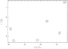 |
Fig. 15 Fraction of detected channels in the WIDEX spectrum of each core vs. the ratio between the mean intensity in the detected channels and the noise of the corresponding spectrum. The names of the cores are indicated inside the points. |
5.2 Comparison with other high-mass star-forming regions
The scenario depicted above is reminiscent of the case of W33A, investigated by Maud et al. (2017). Both sources, when observed at higher resolution, reveal a cluster of cores, possibly in different evolutionary phases, and do not present irrefutable evidence of Keplerian rotation, although the presence of disks on smaller scales is suggested in W33A by detailed modeling (Izquierdo et al. 2018). Also, in W33A accretion onto the cores appears to proceed through a spiral-like filament, while in our case the line profiles hint at infall onto most of the cores. Despite these similarities, there are also differences between IRAS 23385+6053 and W33A, the most important of which are the spatial scales investigated in the two cases. The spatial resolution is approximately ten times worse in IRAS 23385+6053 (~4400 au) than in W33A (~500 au), and the cores are distributed over a region of ~3500 au in W33A as opposed to ~20000 au in IRAS 23385+6053. Moreover, W33A is approximately 10 times more luminous but approximately 20 times less massive, and seems more chemically rich than IRAS 23385+6053. All these features reinforce our conviction that IRAS 23385+6053 is a young massive cluster in the making, with a (proto)stellar content yet in an early evolutionary phase (as predicted by Molinari et al. 1998, 2008b), whereas W33A represents a more evolved stage.
More similar to our source is probably IRAS 05358+3543, where at least four protostellar cores have been identified by Beuther et al. (2007). Although the spatial resolution is ~900 au, better than in our case, the core cluster spans a region of ~16000 au, similar to IRAS 23385+6053. The bolometric luminosity (~ 6 × 10³ L⊙) and total mass of all cores (~34 M⊙; see Table 3 of Beuther et al. 2007) are also similar to those of our source. Despite these similarities, the two objects also present two substantial differences: no free–free continuum emission has been detected from the cores in IRAS 23385+6053, whereas a hypercompact H II region is found in IRAS 05358+3543; and multiple outflows are known to be associated with the cores in this source, unlike our case where only questionable evidence of two bipolar outflows has been found. These differences seem to suggest that IRAS 05358+3543 is in a more advanced stage with respect to IRAS 23385+6053. However, one should keep in mind that no deep, sub-arcsecond continuum observation at centimeter wavelengths has been performed towards IRAS 23385+6053. It is worth noting that the presence of the two H II regions shown in Fig. 1 could make it difficult to detect faint free–free continuum emission from any putative hypercompact H II region deeply embedded in one of the cores.
6 Summary and conclusions
In the context of the CORE project (PI Henrik Beuther) we have performed observations of the continuum and molecular line emission at ~1.4 mm from the high-mass star-forming region IRAS 23385+6053. This is believed to be the youngest of the whole CORE sample. We have revealed six cores and possibly an outflow from a low-mass star. One of the cores (A1) could contain a self-gravitating disk rotating about a ~9 M⊙ star, responsible for most of the 3000 L⊙ estimated for IRAS 23385+6053. The other cores are less massive and colder, but all of them appear to be on the edge of collapse. The accretion rates estimated from the velocity dispersions are consistent with those typical of high-mass star-forming regions. We conclude that IRAS 23385+6053 contains a sample of cores that are forming, or are bound to form, a cluster of massive stars.
Acknowledgements
It is a pleasure to thank Daniele Galli for stimulating discussions and Sergio Molinari for criticallyreading the manuscript. We thank the IRAM technical staff for their support in this project. DS acknowledges support by the Deutsche Forschungsgemeinschaft through SPP 1833: “Building a Habitable Earth” (SE 1962/6-1). H.B., A.A., J.C.M., and S.S. acknowledge support from the European Research Council under the Horizon 2020 Framework Program via the ERC Consolidator Grant CSF-648505. R.K. acknowledges financial support via the Emmy Noether Research Group on Accretion Flows and Feedback in Realistic Models of Massive Star Formation funded by the German Research Foundation (DFG) under grant no. KU 2849/3-1 and KU 2849/3-2. A.P. acknowledges financial support from UNAM-PAPIIT IN113119 grant, México. R.G.M. acknowledges support from UNAM-PAPIIT Programme IN104319. This work is based on observations carried out under project number L14AB008 with the IRAM interferometer and 30-m telescope. IRAM is supported by INSU/CNRS (France), MPG (Germany) and IGN (Spain). XCLASS development is supported by BMBF/Verbundforschung through the Projects ALMA-ARC 05A11PK3 and 05A14PK1 and through ESO Project 56787/14/60579/HNE.
References
- Ahmadi, A., Beuther, H., Mottram, J. C., et al. 2018, A&A, 618, A46 [NASA ADS] [CrossRef] [EDP Sciences] [Google Scholar]
- Bachiller, R., Liechti, S., Walmsley, C. M., & Colomer, F. 1995, A&A, 295, L51 [NASA ADS] [Google Scholar]
- Ballesteros-Paredes, J., Hartmann, L. W., Vázquez-Semadeni, E., Heitsch, F., & Zamora-Avilés, M. A. 2011, MNRAS, 411, 65 [NASA ADS] [CrossRef] [Google Scholar]
- Beltrán, M. T., & de Wit, W. J. 2016, A&ARv, 24, 6 [NASA ADS] [CrossRef] [Google Scholar]
- Bertin, G., & Lodato, G. 1999, A&A, 350, 694 [NASA ADS] [Google Scholar]
- Beuther, H., Leurini, S., Schilke, P., et al. 2007, A&A, 466, 1065 [NASA ADS] [CrossRef] [EDP Sciences] [Google Scholar]
- Beuther, H., Mottram, J. C., Ahmadi, A., et al. 2018, A&A, 617, A100 [NASA ADS] [CrossRef] [EDP Sciences] [Google Scholar]
- Bosco, F., Beuther, H., Ahmadi, A., et al. 2019, A&A, submitted [Google Scholar]
- Busquet, G., Lefloch, B., Benedettini, M., et al. 2014, A&A, 561, A12 [Google Scholar]
- Cesaroni, R. 2005, in Massive star birth: A crossroads of Astrophysics, eds. R. Cesaroni, M. Felli, E. Churchwell, & M. Walmsley, IAU Symp., 227, 59 [NASA ADS] [CrossRef] [Google Scholar]
- Cesaroni, R., Neri, R., Olmi, L., et al. 2005, A&A, 434, 1039 [NASA ADS] [CrossRef] [EDP Sciences] [Google Scholar]
- Cesaroni, R., Sánchez-Monge, Á., Beltrán, M. T., et al. 2017, A&A, 602, A59 [NASA ADS] [CrossRef] [EDP Sciences] [Google Scholar]
- Douglas, T. A., Caselli, P., Ilee, J. D., et al. 2013, MNRAS, 433, 2064 [NASA ADS] [CrossRef] [Google Scholar]
- Faustini, F., Molinari, S., Testi, L., & Brand, J. 2009, A&A, 503, 801 [NASA ADS] [CrossRef] [EDP Sciences] [Google Scholar]
- Field, G. B., Blackman, E. G., & Keto, E. R. 2011, MNRAS, 416, 710 [NASA ADS] [Google Scholar]
- Fontani, F., Cesaroni, R., Testi, L., et al. 2004, A&A, 414, 299 [NASA ADS] [CrossRef] [EDP Sciences] [Google Scholar]
- Gerner, T., Beuther, H., Semenov, D., et al. 2014, A&A, 563, A97 [NASA ADS] [CrossRef] [EDP Sciences] [Google Scholar]
- Ilee, J. D., Cyganowski, C. J., Brogan, C. L., et al. 2018, ApJ, 869, L24 [NASA ADS] [CrossRef] [Google Scholar]
- Izquierdo, A. F., Galván-Madrid, R., Maud, L. T., et al. 2018, MNRAS, 478, 2505 [NASA ADS] [CrossRef] [Google Scholar]
- Kalenskii, S. V., & Kurtz, S. 2016, Astron. Rep., 60, 702 [NASA ADS] [CrossRef] [Google Scholar]
- Kurtz, S., Cesaroni, R., Churchwell, E., Hofner, P., & Walmsley, C.M. 2000, in Protostars and Planets IV, eds. V. Mannings, A. Boss & S. Russel (Tucson: University of Arizona Press), 299 [Google Scholar]
- Kurtz, S., Hofner, P., & Álvarez, C. V. 2004, ApJS, 155, 149 [NASA ADS] [CrossRef] [Google Scholar]
- Leurini, S., Codella, C., Zapata, L., et al. 2011, A&A, 530, A12 [NASA ADS] [CrossRef] [EDP Sciences] [Google Scholar]
- Li, J., Myers, P. C., Kirk, H., et al. 2019, ApJ, 871, 163 [NASA ADS] [CrossRef] [Google Scholar]
- MacLaren, I., Richardson, K. R., & Wolfendale, W. 1988, ApJ, 333, 821 [NASA ADS] [CrossRef] [Google Scholar]
- Mardones, D., Myers, P. C., Tafalla, M., et al. 1997, ApJ, 489, 719 [NASA ADS] [CrossRef] [Google Scholar]
- Maud, L. T., Moore, T. J. T., Lumsden, S. L., et al. 2015, MNRAS, 453, 645 [NASA ADS] [CrossRef] [Google Scholar]
- Maud, L. T., Hoare, M. G., Galván-Madrid, R., et al. 2017, MNRAS, 467, L120 [NASA ADS] [Google Scholar]
- Mayen-Gijon, J. M., Anglada, G., Osorio, M., et al. 2014, MNRAS, 437, 3766 [NASA ADS] [CrossRef] [Google Scholar]
- Möller, T., Endres, C., & Schilke, P. 2017, A&A, 598, A7 [NASA ADS] [CrossRef] [EDP Sciences] [Google Scholar]
- Molinari, S., Brand, J., Cesaroni, R., & Palla, F. 1996, A&A, 308, 573 [NASA ADS] [Google Scholar]
- Molinari, S., Testi, L., Brand, J., Cesaroni, R., & Palla, F. 1998, ApJ, 505, L39 [NASA ADS] [CrossRef] [Google Scholar]
- Molinari, S., Testi, L., Rodríguez, L. F., & Zhang, Q. 2002, ApJ, 570, 758 [NASA ADS] [CrossRef] [Google Scholar]
- Molinari, S., Pezzuto, S., Cesaroni, R., et al. 2008a, A&A, 481, 345 [NASA ADS] [CrossRef] [EDP Sciences] [Google Scholar]
- Molinari, S., Faustini, F., Testi, L., et al. 2008b, A&A, 487, 1119 [NASA ADS] [CrossRef] [EDP Sciences] [Google Scholar]
- Mottram, J. C., Hoare, M. G., Davies, B., et al. 2011, ApJ, 730, L33 [NASA ADS] [CrossRef] [Google Scholar]
- Mottram, J. C., Beuther, H., Ahmadi, A., et al. 2019, A&A, submitted [Google Scholar]
- Ohashi, S., Sanhueza, P., Sakai, N., et al. 2018, ApJ, 856, 147 [NASA ADS] [CrossRef] [Google Scholar]
- Ossenkopf, V., & Henning, Th. 1991, A&A, 291, 943 [Google Scholar]
- Palau, A., Ballesteros-Paredes, J., Vázquez-Semadeni, E., et al. 2015, MNRAS, 453, 3785 [NASA ADS] [CrossRef] [Google Scholar]
- Palau, A., Walsh, C., Sánchez-Monge, Á., et al. 2017, MNRAS, 467, 2723 [NASA ADS] [Google Scholar]
- Palau, A., Zapata, Luis, A., Román-Zú niga, C. G., et al. 2018, ApJ, 855, 24 [NASA ADS] [CrossRef] [Google Scholar]
- Palla, F., Brand, J., Cesaroni, R., Comoretto, G., & Felli, M. 1991, A&A, 246, 249 [NASA ADS] [Google Scholar]
- Schuller, A., Menten, K. M., Contreras, Y., et al. 2009, A&A, 504, 415 [NASA ADS] [CrossRef] [EDP Sciences] [Google Scholar]
- Wolf-Chase, G., Smutko, M., Sherman, R., Harper, D. A., & Medford, M. 2012, ApJ, 745, 116 [NASA ADS] [CrossRef] [Google Scholar]
- Wu, Y., Zhang, Q., Chen, H., et al. 2005, ApJ, 129, 330 [Google Scholar]
- Zhang, Q., Hunter, T. R., Brand, J., et al. 2001, ApJ, 552, L167 [NASA ADS] [CrossRef] [Google Scholar]
- Zhang, Q., Hunter, T. R., Brand, J., et al. 2005, ApJ, 625, 864 [NASA ADS] [CrossRef] [Google Scholar]
If the emission is thin, the ratio between the brightness temperatures of two lines is equal to the ratio between the corresponding optical depths, therefore: ![Mathematical equation: $T_{\textrm{B}}^2/T_{\textrm{B}}^1\simeq [(S\mu^2)_2/(S\mu^2)_1)] \, (\nu_2/\nu_1) \, \exp[-(E_2-E_1)/T] < [(S\mu^2)_2/(S\mu^2)_1)] \, (\nu_2/\nu_1) \simeq 0.56$](/articles/aa/full_html/2019/07/aa35506-19/aa35506-19-eq25.png) , where the line strengths and frequencies are given in Table 1.
, where the line strengths and frequencies are given in Table 1.
XCLASS is available at https://xclass.astro.uni-koeln.de
The velocity is obtained as half the difference between the velocities observed at the blueshifted (~–51 km s−1) and redshifted (~–50 km s−1) peaks located along the dotted line in Fig. 10.
Our approach of including the ram pressure in the external pressure on the core surface is not strictly correct in the hydrostatic scenario of Field et al. (2011). However, it has been shown by Ballesteros-Paredes et al. (2011) that such an approach yields results comparable to those obtained from the correct treatment of infall.
With “massive cluster” here we mean a stellar cluster with at least one massive (O-type or early B-type) YSO.
All Tables
All Figures
|
Fig. 1 Panel a: map of the emission integrated over the 13CO(2–1) line (solid contours) overlaid on an image of the continuum emission at 24 μm (from Molinari et al. 2008b). The latter has an angular resolution of 6′′. The 13 CO map was obtained with the IRAM 30-m data at a resolution of 12′′ (the beam is shown in the bottom left corner). Solid contour levels range from 20 to 84 in steps of 8 K km s−1. The dotted contours represent a map of the 3.6 cm continuum emission imaged with the VLA Molinari et al. (2002) and range from 0.5 to 2.3 in steps of 0.3 mJy beam−1. The synthesized beam is 10′′.2 × 9′′.0 with PA = −59°. Panel b: same as top panel, where solid contours are a map of the emission averaged over the 13 CO(2–1) line, obtained after merging the NOEMA with the IRAM 30-m data. The resulting synthesized beam is 0′′. 49×0′′.44 with PA = 57° (shown in the bottom left corner). The circle corresponds to the half-power beam width of the NOEMA antennas. The contour levels range from 36 to 144 in steps of 18 mJy beam−1. |
| In the text | |
|
Fig. 2 Map of the 1.4 mm continuum emission from IRAS 23385+6053. The values of the contour levels are marked in the color scale to the right. The minimum contour level (0.55 mJy beam−1) corresponds to 5σ. The crosses indicate the positions of the three cores identified by BEU18, corresponding to A1, B, and E in Table 1. |
| In the text | |
|
Fig. 3 Spectrum obtained with the WIDEX correlator at low spectral resolution towards the peak of core A1. Only the strongest molecular transitions are indicated. The red color denotes the lines observed also at high spectral resolution. |
| In the text | |
|
Fig. 4 Maps of the mean emission in various molecular lines. For the sake of direct comparison with the line maps we show again the map of the continuum emission in the bottom right panel. For each map, the values of the contour levels are marked in the corresponding color scale. The crosses and letters indicate the positions of the six cores identified by us (see also Fig. 5). Cores A1, B, and E correspond to the crosses in Fig. 2. The ellipse in the bottom right of each panel is the synthesized beam. |
| In the text | |
|
Fig. 5 Sketch of the cores identified by us in IRAS 23385+6053. The contour corresponds to the 5σ level of the continuum emission. The two arrows and arcs indicate the direction and location of the expanding lobes (F1 and F2) of the bipolar outflow detected in the H2 CO and CH3 OH emission, perhaps originating from core C. |
| In the text | |
|
Fig. 6 Same as Fig. 4 but over a larger region and only for the H2 CO and CH3 OH lines. The dashed line denotes the direction defined by the two emission blobs, F1 and F2, located to the SE and NW of the main cores, respectively. |
| In the text | |
|
Fig. 7 Panel a: map of the zero moment (integrated intensity; contours) of the CH3 OH(42–31) E1 line overlaid on the map (color image) of the first moment of the same transition. Contour levels range from 0.05 to 1.25 in steps of 0.2 Jy beam−1 km s−1. The ellipse in the bottom right represents the synthesized beam. The dashed line has the same meaning as in Fig. 6. Panel b: same as top panel, but for the second moment of the methanol line. |
| In the text | |
|
Fig. 8 Maps of the CH3OH rotational temperature (color image) and column density (contours) obtained with the XCLASS program. The labels indicate the cores. Contour levels range from 2 × 10¹⁵ to 1.1 × 10¹⁶ in steps of 1015 cm−2. Typical uncertainties on the values of the rotational temperature are 10–20%. The ellipse in the bottom left denotes the synthesized beam. The dashed box corresponds to the region shown in Fig. 9. |
| In the text | |
|
Fig. 9 Maps of the CH3CN rotational temperature (color image) and column density (contours) obtained with the XCLASS program. The labels have the same meaning as in Fig. 4. Contour levels range from 2 × 10¹³ to 1014 in steps of 1013 cm−2. Typical uncertainties on the values of the rotational temperature are 10–20%. |
| In the text | |
|
Fig. 10 Map of the CH3CN(12–11) line emissionaveraged over the K = 0 and 1 components (contours) overlaid on the map of the velocity in the same line, obtained by simultaneously fitting the K = 0–4 components as explained in the text. Labels A1 and A2 mark the center positions of the corresponding cores. Contour levels range from 9.5 (5σ) to 57 in steps of 9.5 mJy beam−1. The dotted and dashed LINES indicate the approximate directions of the two velocity gradients. |
| In the text | |
|
Fig. 11 Model velocity map for a geometrically thin disk undergoing both Keplerian rotation and expansion with radial velocity proportional to the radius. Fiducial values have been assumed for the parameters (see text). The map has been rotated by 45° to ease the comparison with Fig. 10. The dotted and dashed lines indicate the directions of the two velocity gradients defined by the blue- and redshifted velocity peaks. |
| In the text | |
|
Fig. 12 Line intensity as a function of velocity and position along the dashed line in Fig. 10 (position angle −56°). Different colors correspond to different molecular species as indicated in the bottom right. The cross in the bottom left gives the velocity and angular resolution. The arrows indicate the possible “spurs” typical of the pattern corresponding to Keplerian rotation. The yellow butterfly-shaped curve is the region inside which emission is expected for a Keplerian disk rotating about an 8 M⊙ star. Contour levels range from 15 (5σ) to 123 in steps of 18 mJy beam−1 for OCS, from 17.5 (5σ) to 332.5 in steps of 52.5 mJy beam−1 for CH3 OH, and from 13.2 (4σ) to 151.8 in steps of 19.8 mJy beam−1 for HC3 N. |
| In the text | |
|
Fig. 13 Line intensity as a function of velocity and position along the dashed line in Fig. 6 (position angle –56°). Different colors correspond to different molecular species as indicated in the bottom right. The cross in the bottom left gives the velocity and angular resolution. The dotted vertical line marks the position of core C, while the dashed line outlines the velocity trend observed in the H2 CO and CH3 OH lines. Contour levels range from 15 (5σ) to 225 in steps of 30 mJy beam−1 for CH3 OH, from 18 (5σ) to 338 in steps of 40 mJy beam−1 for H2 CO, and from 16 (4σ) to 32 in steps of 3 mJy beam−1 for H2 CCO. |
| In the text | |
|
Fig. 14 Spectra of the H2CO(303–202) (black solid histogram) and CH3OH(42–31) E1 (red dashed histogram) lines towards the positions of the six cores identified in IRAS 23385+6053. The vertical dotted line is shown to ease the comparison between spectra of different cores. |
| In the text | |
|
Fig. 15 Fraction of detected channels in the WIDEX spectrum of each core vs. the ratio between the mean intensity in the detected channels and the noise of the corresponding spectrum. The names of the cores are indicated inside the points. |
| In the text | |
Current usage metrics show cumulative count of Article Views (full-text article views including HTML views, PDF and ePub downloads, according to the available data) and Abstracts Views on Vision4Press platform.
Data correspond to usage on the plateform after 2015. The current usage metrics is available 48-96 hours after online publication and is updated daily on week days.
Initial download of the metrics may take a while.