| Issue |
A&A
Volume 679, November 2023
|
|
|---|---|---|
| Article Number | A108 | |
| Number of page(s) | 17 | |
| Section | Interstellar and circumstellar matter | |
| DOI | https://doi.org/10.1051/0004-6361/202347060 | |
| Published online | 17 November 2023 | |
JOYS: Disentangling the warm and cold material in the high-mass IRAS 23385+6053 cluster
1
Max Planck Institute for Extraterrestrial Physics,
Gießenbachstraße 1,
85749
Garching bei München, Germany
e-mail: This email address is being protected from spambots. You need JavaScript enabled to view it.
2
Max Planck Institute for Astronomy,
Königstuhl 17,
69117
Heidelberg, Germany
3
Leiden Observatory, Leiden University,
PO Box 9513,
2300 RA
Leiden, The Netherlands
4
European Southern Observatory,
Karl-Schwarzschild-Strasse 2,
85748
Garching bei München, Germany
5
Department of Experimental Physics, Maynooth University-National University of Ireland Maynooth,
Maynooth, Co Kildare, Ireland
6
INAF-Osservatorio Astronomico di Capodimonte,
Salita Moiariello 16,
80131
Napoli, Italy
7
Dublin Institute for Advanced Studies,
31 Fitzwilliam Place,
D02 XF86
Dublin, Ireland
8
UK Astronomy Technology Centre, Royal Observatory Edinburgh,
Blackford Hill,
Edinburgh
EH9 3HJ, UK
9
Department of Space, Earth and Environment, Chalmers University of Technology,
Onsala Space Observatory,
439 92
Onsala, Sweden
10
Laboratory for Astrophysics, Leiden Observatory, Leiden University,
PO Box 9513,
NL 2300 RA
Leiden, The Netherlands
11
Centro de Astrobiologia (CAB, CSIC-INTA), Carretera de Ajalvir,
8850
Torrejon de Ardoz, Madrid, Spain
12
Department of Astrophysics, University of Vienna,
Türkenschanzstr. 17,
1180
Vienna, Austria
13
ETH Zürich, Institute for Particle Physics and Astrophysics,
Wolfgang-Pauli-Str. 27,
8093
Zürich, Switzerland
14
Université Paris-Saclay, Université de Paris, CEA, CNRS, AIM,
91191
Gif-sur-Yvette, France
15
Department of Astronomy, Oskar Klein Centre, Stockholm University,
106 91
Stockholm, Sweden
16
Instituut voor Sterrenkunde, KU Leuven,
Celestijnenlaan 200D,
Bus-2410,
3000
Leuven, Belgium
Received:
31
May
2023
Accepted:
18
September
2023
Abstract
Context. High-mass star formation occurs in a clustered mode where fragmentation is observed from an early stage onward. Young protostars can now be studied in great detail with the recently launched James Webb Space Telescope (JWST).
Aims. We study and compare the warm (>100 K) and cold (<100 K) material toward the high-mass star-forming region (HMSFR) IRAS 23385+6053 (IRAS 23385 hereafter) combining high-angular-resolution observations in the mid-infrared (MIR) with the JWST Observations of Young protoStars (JOYS) project and with the NOrthern Extended Millimeter Array (NOEMA) at millimeter (mm) wavelengths at angular resolutions of ≈0.″2–1.″0.
Methods. We investigated the spatial morphology of atomic and molecular species using line-integrated intensity maps. We estimated the temperature and column density of different gas components using H2 transitions (warm and hot component) and a series of CH3CN transitions as well as 3 mm continuum emission (cold component).
Results. Toward the central dense core of IRAS 23385, the material consists of relatively cold gas and dust (≈50 K), while multiple outflows create heated and/or shocked H2 and show enhanced temperatures (≈400 K) along the outflow structures. An energetic outflow with enhanced emission knots of [Fe II] and [Ni II] suggests J-type shocks, while two other outflows have enhanced emission of only H2 and [S I] caused by C-type shocks. The latter two outflows are also more prominent in molecular line emission at mm wavelengths (e.g., SiO, SO, H2CO, and CH3OH). Data of even higher angular resolution are needed to unambiguously identify the outflow-driving sources given the clustered nature of IRAS 23385. While most of the forbidden fine structure transitions are blueshifted, [Ne II] and [Ne III] peak at the source velocity toward the MIR source A/mmA2 suggesting that the emission is originating from closer to the protostar.
Conclusions. The warm and cold gas traced by MIR and mm observations, respectively, are strongly linked in IRAS 23385. The outflows traced by MIR H2 lines have molecular counterparts in the mm regime. Despite the presence of multiple powerful outflows that cause dense and hot shocks, a cold dense envelope still allows star formation to further proceed. To study and fully understand the spatially resolved MIR properties, a representative sample of low- and high-mass protostars has to be probed using JWST.
Key words: stars: formation / ISM: individual objects: IRAS 23385+6053 / stars: jets / stars: massive
© The Authors 2023
 Open Access article, published by EDP Sciences, under the terms of the Creative Commons Attribution License (https://creativecommons.org/licenses/by/4.0), which permits unrestricted use, distribution, and reproduction in any medium, provided the original work is properly cited.
This article is published in open access under the Subscribe to Open model.
Open Access funding provided by Max Planck Society.
1 Introduction
Despite having been studied for many decades, the formation of high-mass stars (stellar masses M* > 8 M⊙) still remains a puzzle; we refer to Motte et al. (2018) and Rosen et al. (2020) for recent reviews. High-mass star-forming regions (HMSFRs) are typically located at distances of several kiloparsecs and in order to achieve a spatial resolution of a few thousand astronomical units (au), subarcsecond resolution is necessary.
With the recently launched James Webb Space Telescope (JWST), infrared(IR)-bright protostars can be characterized at subarcsecond resolution and high sensitivity in the near-infrared (NIR) and mid-infrared (MIR) regimes. The observations analyzed in this work are part of the European Consortium guaranteed time program JWST Observations of Young protoStars (JOYS, PI: E. F. van Dishoeck, id. 1290). The project targets low-mass and high-mass protostars with the Mid-InfraRed Instrument (MIRI) using the Medium Resolution Spectrometer (MRS) mode. The first target observed as part of the JOYS project is the HMSFR IRAS 23385+6053 (IRAS 23385 hereafter), also referred to as Mol 160 (Molinari et al. 1996).
IRAS 23385 is associated with H2O maser activity (Molinari et al. 1996), but remains undetected at centimeter (cm) wavelengths (Molinari et al. 1998a). This suggests that IRAS 23385 is at an evolutionary stage prior to the ultracompact (UC) H II region phase (Molinari et al. 1998b). The mass of the central object and the envelope are estimated to be ≈9 M⊙ (Cesaroni et al. 2019) and 510 M⊙ (Beuther et al. 2018), respectively. Molinari et al. (1998b) derived a mean visual extinction of the core of AV = 200 mag with a H2 column density N(H2) of 2 × 1024 cm−2.
The Two Micron All Sky Survey (2MASS) data toward the region reveal that the dense core is surrounded by NIR sources and is located in between two UCHII regions with bright cm emission (Molinari et al. 2002; Thompson & Macdonald 2003). A large-scale overview toward the region is shown in Fig. 1 and highlights the 250 μm, 70 μm, and 24 μm images in the region taken with the Herschel and Spitzer space telescopes. The central region is labeled “mm”, while the two nearby UCHII regions are labeled “VLA1” and “VLA2” (Molinari et al. 2002). Large-scale filamentary cold dust emission is revealed by the Herschel 250 μm data. The Herschel 70 μm and Spitzer 24 μm data reveal an emission arc between the UCHII region VLA2 and the mm core.
Molinari et al. (2008) detect faint 24 μm emission (with a flux density of  ) toward the position of the central dense core (their source “A”), but no emission at lower wavelengths, confirming the pre-zero-age main sequence (ZAMS) nature of the source. By modeling the spectral energy distribution (SED), the authors derive a bolometric luminosity of L = 3.2 × 10³ L⊙ for the core, while the luminosity of the entire region, that is, including the two nearby bright UCHII regions (Fig. 1), is L = 1.6 × 10⁴ L⊙ (Molinari et al. 1998b).
Bipolar outflows are found in broad line wings in CO emission (southwest(redshifted)-northeast(blueshifted), Wu et al. 2005) and in SiO and HCO+ emission (north(redshifted)– south(blueshifted), Molinari et al. 1998b). As the emission is not extended and the outflow lobes overlap, Molinari et al. (1998b) conclude that the direction of the north-south outflow is nearly pole-on.
IRAS 23385 is part of the NOrthern Extended Millimeter Array (NOEMA) large program “CORE” (PI: H. Beuther), the aim of which is to image the central dense core at an angular resolution of 0.″5 at 1 mm (Beuther et al. 2018). Cesaroni et al. (2019) carried out a case study toward IRAS 23385 using the CORE data and suggested the presence of a northwest (redshifted)–southeast(blueshifted) outflow. These authors, based on the observed IR, mm, and cm emission, concluded that a cluster of massive stars is probably being formed in the central core of IRAS 23385.
While interferometric mm observations trace the cold material, the presence of outflows and MIR emission suggests an additional warm component that is heated by the protostars and/or shocks. As a homonuclear diatomic, the most abundant molecule in the interstellar medium, H2, has no permanent dipole and therefore lacks pure rotational dipole transitions. However, ro-vibrational quadrupole transitions of H2 can be excited at high temperatures, with upper energy levels of Eu/kB > 500 K. Such transitions can be accessed with JWST/MIRI for H2 that covers the ΔJ = 0 rotational lines in the vibrational ground state 0–0 from S(1) to S(7) (Table 1). In addition, JWST/MIRI covers emission lines from neutral and ionized atoms and molecules.
The first JOYS results for IRAS 23385 using JWST/MIRI MRS data are presented in Beuther et al. (2023). Toward the central dense core, two MIR sources are detected at short wavelengths that become unresolved at longer wavelengths (λ ≳ 15 μm). Aside from continuum emission, the MIRI spectrum from 5 to 28 μm is dominated by emission of H2 lines and forbidden transitions of atomic lines tracing the MIR sources and multiple outflows. In addition, the spectrum shows deep absorption features by ice species. The continuum emission at 24 μm rises to ≃0.1–0.2 Jy, a similar value derived from past Spitzer data (0.14 Jy, Molinari et al. 2008). Using a faint Humphreys α line, an accretion rate of 0.9×10⁻⁴ M⊙ yr−1 is estimated (Beuther et al. 2023). Compact molecular line emission toward the MIR sources is being studied by Francis et al. (in prep.) and the ice properties will be presented in Rocha et al. (in prep.); see also van Dishoeck et al. (2023).
In the present work, we characterize and compare the warm and cold material in detail for the first time, taking advantage of new JWST/MIRI MRS observations that can be compared with NOEMA data at mm wavelengths and used to study the nature of the continuum sources. With NOEMA, the cold molecular gas and dust properties can be studied, while with JWST/MIRI observations we probe the warmer environment. In Sect. 2, the observational parameters and calibration of the JWST and NOEMA data are explained. An analysis of the continuum and spectral line data is presented in Sect. 3, and in Sect. 4 the results are discussed. Our conclusions are summarized in Sect. 5.
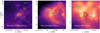 |
Fig. 1 Multi-wavelength overview of IRAS 23385. In color, the Herschel 250 μm (left), Herschel 70 μm (center), and Spitzer 24 μm (right) emission are shown in log-scale. The gray dashed squares show the field of view of the following panel. In the center and right panels, the green star labeled “mm” marks the 1 mm continuum peak position (Fig. 2). The blue stars labeled “VLA1” and “VLA2” show the position of the two nearby UCHII regions (Molinari et al. 2002). The black rectangles in the right panel indicate the JWST/MIRI MRS field of view of the four-pointing mosaic in ch1A (solid) and ch4C (dashed). |
MIR lines covered by JWST/MIRI MRS.
2 Observations
In this work, we analyze line and continuum observations at MIR wavelengths with JWST/MIRI (Sect. 2.1) and at 1 mm and 3 mm with NOEMA observations (Sect. 2.2). With angular resolutions of 0.″2−1″, spatial scales down to ≈ 1000–5000 au can be traced in IRAS 23385, at a distance of 4.9 kpc.
The kinematic distance is estimated to be 4.9 kpc (Molinari et al. 1998b) with a Local Standard of Rest (LSR) velocity of vLSR = −50.2 km s−1 (Beuther et al. 2018). Typically, kinematic distance estimates suffer from high uncertainties. Molinari et al. (2008) modeled the SED with a ZAMS star embedded in an envelope but were unsuccessful in properly explaining the observed SED. The authors argued that the region may actually be located at 8 kpc or that the source is at a younger evolutionary stage. On the other hand, using the Galactic rotation curve and spiral arm model by Reid et al. (2016, 2019), a distance of 2.7±0.2 kpc could be estimated1. However, this distance estimate includes an association with a spiral arm as a prior. Maser parallax measurements are not available for this source. Choi et al. (2014) measured maser parallaxes toward high-mass star-forming regions and compared the corresponding distances with kinematic distance estimates finding significant discrepancies. The authors concluded that for G111.23−1.23 – the source in their sample that is closest to IRAS 23385 and has a similar vLSR – the kinematic distance is 4.8 kpc (vLSR = –53 km s−1), while the maser parallax measurement suggests a distance of 3.33 kpc. However, as IRAS 23385 is not covered by Choi et al. (2014), and given the uncertainties, we assume in this work a distance of 4.9 kpc, which is consistent with previous studies in the literature and in line with the distance used by the JOYS team (Beuther et al. 2023). The high uncertainty in distance does not affect the analysis in this work.
2.1 JWST
The observations were carried out on August 22, 2022, with a total observing time of 2.12 h (40 min on source) and a mosaic of four pointings surrounding the dense core in IRAS 23385. The MIRI MRS instrument consists of four channels (ch1, ch2, ch3, ch4) and each of them is divided intro three sub-bands (short, medium, and long), which we refer to as A, B, and C. The total spectral coverage ranges from 4.9 to 27.9 μm with a resolving power R decreasing from 3 700 to 1 300 (Wells et al. 2015; Labiano et al. 2021; Argyriou et al. 2023; Jones et al. 2023).
The angular resolution can be estimated as θ = 0.033λ(μm) + 0.″106 (Law et al. 2023) and the field of view (FoV) of the four-pointing mosaic increases from ≈7″ × 7″ to ≈ 15″ × 15″ from short to long wavelengths (Fig. 1). The slice width of MIRI MRS increases from 0.″176 to 0.″645 from ch1 to ch4 (Wells et al. 2015).
The observations were calibrated using the JWST Science Calibration Pipeline (version 1.11.2) and Calibration Reference Data System (CRDS) context “jwst_1100.pmap”. In addition, astrometric corrections were applied by comparing detected sources in the Gaia data (Gaia Collaboration 2021) with those detected in the MIRI imaging field, which was observed simultaneously using MIRI. We refer to Beuther et al. (2023) for a detailed description of the calibration of this data set.
The resulting spectral cube data product consists of continuum and line emission, as well as ice absorption features. In this work, we focus on the extended H2 emission and forbidden atomic fine structure transitions. Table 1 provides an overview of all lines that are analyzed in this work. With a spectral resolution of a few tens of km s−1, the high-velocity outflow components can be resolved (Beuther et al. 2023), but a detailed kinematic analysis of the gas properties close to the protostars is difficult. Thus, in this work we focus on the spatial distribution of the integrated emission.
A 5.2 μm continuum map is created using the ch1A band at a wavelength range of between 5.2 μm and 5.3 μm, in which bright line emission or absorption features are absent. The angular resolution is ≈0.″2. Faint extended background emission with a median of 48 MJy sr−1 is subtracted from the 5.2 μm intensity map. The noise measured as the standard deviation of the 5.2 μm continuum map is 18 MJy sr−1 after background subtraction.
In individual line cubes (Table 1), the local continuum was subtracted by fitting a first-order polynomial to the spectra masking out channels with line emission. The line noise, σline, is estimated in line-free channels and decreases from 38 MJy sr−1 to 5 MJy sr−1 from ch1A to ch3C and then increases again up to 32 MJy sr−1 in ch4C.
2.2 NOEMA
Located in the Northern hemisphere, with a high declination of ≈61°, IRAS 23385 is most accessible at high angular resolution at mm wavelengths with the NOrthern Extended Millimeter Array (NOEMA).
2.2.1 1 mm data
IRAS 23385 is included in the sample of the NOEMA large program CORE (Beuther et al. 2018; Gieser et al. 2021; Ahmadi et al. 2023, PI: H. Beuther, project code L14AB). The region was observed with NOEMA in the D, A, and C configurations in January 2015, February 2016, and October 2016, respectively. The WideX correlator provides a spectral coverage from 217.2 GHz to 220.8 GHz (1.36–1.38 mm) at an angular resolution of ≈0.″5. High-resolution data with a channel width, δv, of 0.5 km s−1 are available for a few targeted molecular lines (Table 2 and 3 in Ahmadi et al. 2018). A continuous spectrum along the full bandwidth is available with a channel width of 3.0 km s−1. For the spectral line data, complementary short spacing observations with the IRAM 30 m telescope were obtained recovering missing flux filtered out by the interferometer. The combination of the interferometric and single-dish (“merged”) data is explained in Mottram et al. (2020).
The NOEMA data were calibrated using the CLIC package in GILDAS2. The interferometric line and continuum data were self-calibrated in order to increase the signal-to-noise (S/N) ratio. Phase self-calibration was performed on the continuum data and then applied to the spectral line data. A detailed description of the self-calibration procedure for the NOEMA data can be found in Gieser et al. (2021).
The NOEMA continuum and continuum-subtracted merged spectral line data were deconvolved using the GILDAS/MAPPING package and the Clark algorithm. The weighting was set to a robust parameter of 0.1 to achieve the highest possible angular resolution. For the 1 mm continuum data, the resulting synthesized beam (with major and minor axis θmaj × θmin) is 0.″48 × 0.″43 with a position angle (PA) of 58°. The continuum noise is estimated to be σcont,1mm = 0.15 mJy beam−1.
The properties of the 1 mm molecular lines presented in this work are summarized in Table 2 with the label “CORE” in the NOEMA project column. The line sensitivity σline, estimated in channels without line emission, is ≈1.2 and ≈0.4 K in the high- and low-spectral-resolution data, respectively, at an angular resolution of ≈0.″5.
Molecular lines covered by NOEMA at 1 mm and 3 mm analyzed in this work.
2.2.2 3 mm data
Using the upgraded PolyFiX correlator at NOEMA, CORE+ (PI: C. Gieser, project code W20AV) is a follow-up project of CORE targeting the 3 mm wavelength range. In a first case study, three regions of the CORE sample were selected, including IRAS 23385 (Gieser et al., in prep.). The NOEMA 3 mm observations were obtained in the A and D configuration and short-spacing information was provided by complementary IRAM 30 m observations. The observations were carried out from February to April 2021 with NOEMA and in August 2021 with the IRAM 30 m telescope. Using the high-resolution spectral units, a channel width δν of 0.8 km s−1 is achieved in the merged line data.
Phase self-calibration was performed on the continuum data using the same procedure as in the 1 mm CORE data (Gieser et al. 2021) and the gain solutions were applied to the NOEMA line data. The NOEMA continuum and continuum-subtracted merged spectral line data were deconvolved using the GILDAS/MAPPING package and the Clark algorithm. The weighting was set to a robust parameter of 1 to achieve a compromise between high-angular-resolution and good sensitivity. For the 3 mm continuum data, the resulting synthesized beam is 1.″1 × 0.″85 (PA 47°) and the noise is estimated to be σcont,3mm = 0.020 mJy beam−1.
The properties of the 3 mm molecular lines analyzed in this study are summarized in Table 2 with the label “CORE+” in the last column. The line sensitivity σline at a channel width of 0.8 km s−1 is ≈ 0.2 K.
For all 1 and 3 mm NOEMA continuum and line data products, we apply a primary beam correction taking into account the fact that the noise levels increase toward the edge of the primary beam. The primary beam is ≈22″ and ≈60″ at 1 mm and 3 mm, respectively. A larger FoV is therefore covered in the NOEMA data compared to the four-pointing mosaic JWST/MIRI observations (≈15″ at the longest wavelengths). Given that we aim to compare the MIR and mm data, we only focus here on the central area (≈12″ × 12″) that is also covered by the JWST/MIRI FoV. The upper energy levels Eu/kB of the mm lines vary between 4 and 100 K, which is significantly lower than for the JWST/MIRI transitions (>500 K). Thus, with the NOEMA continuum and line data, we are also able to trace the cold molecular gas in the same region.
3 Results
A comparison of the detected JWST/MIRI MRS and NOEMA mm lines allows us to study the properties of the warm and cold material, respectively, at subarcsecond resolution corresponding to spatial scales below 5000 au for IRAS 23385. In addition, the continuum allows us to map the different sources present in the FoV. In Sect. 3.1, the continuum emission, detected sources, and outflows are presented. The spatial morphology of atomic and molecular line emission is compared in Sect. 3.2. The temperature of the warmer gas (> 100 K) is derived from the JWST/MIRI H2 0−0 lines in Sect. 3.3, while the temperature of the cold gas (< 100 K) is estimated by modeling CH3CN emission lines in Sect. 3.4.
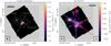 |
Fig. 2 MIR Continuum (left) and H2 0−0 S(7) line emission (right) for IRAS 23385. In the left panel, the JWST/MIRI 5.2 μm continuum with emission >5σcont,5μm is presented in color. Gray contours show the NOEMA 1 mm continuum with contour levels at 5, 10, 20, 40, and 80×σcont,1mm. The dash-dotted white circles show the aperture in which the 5.2 μm flux density F5.2μm was derived (Table 3). In the bottom left corner, the JWST/MIRI 5.2 μm and NOEMA 1 mm angular resolutions are indicated in black and gray, respectively. The mm (mmA1 and mmB, marked by green squares) and MIR (A/mmA2 and B) continuum sources are labeled in green. In the right panel, the line-integrated intensity of the H2 0−0 S(7) line with S/N > 5 is presented in color. The JWST/MIRI 5.2 μm continuum as shown in the left panel is presented as blue contours with contour levels at 5, 10, 15, 20, and 25 × σcont,5μm. The angular resolutions of the 5.2 μm continuum and H2 0−0 S(7) line data are indicated in the bottom left and right, respectively. Several shock spots evident in the MIRI MRS line emission are marked by green crosses and labeled in green (Sect. 3.2). The red and blue arrows indicate three bipolar outflows, labeled I, II, and III (as presented in Beuther et al. 2023). In both panels, the black bar indicates a spatial scale of 10 000 au at the assumed source distance of 4.9 kpc. |
3.1 Continuum sources and outflows
A comparison of the JWST/MIRI 5.2 μm and NOEMA 1 mm continuum data is presented in Fig. 2 in the left panel with detected sources labeled. For the mm and MIR sources, we follow the nomenclature of Cesaroni et al. (2019) and Beuther et al. (2023), respectively.
The 1 mm continuum data clearly resolve two cores (mmA1 and mmB) that are separated by ≈1.″6, corresponding to a projected separation of ≈7700 au. The mmA continuum peak is elongated and can be separated into two sources “mmA1” and “mmA2”.
The 5.2 μm continuum data reveal two sources, A and B, that are barely resolved at an angular resolution of 0.″2. The MIR source A is co-spatial with the elongated mm core “mmA2”, hereafter referred to as “A/mmA2”. While the two sources can be resolved in the shorter wavelength regime of MIRI, beyond ≈ 15 μm this is not possible due to the lower angular resolution (Beuther et al. 2023). Notably, no additional source is detected in the MIRI data at longer wavelengths. The positions of the four continuum sources are summarized in Table 3. In addition, the flux densities at 5.2 μm F5.2μm – calculated within a 0.″5 circular aperture (Fig. 2) – of the MIR sources A/mmA2 and B are listed. For the nondetections of sources mmA1 and mmB, 3σ upper limits are given.
The 1 mm continuum morphology surrounding the cores reveals complex substructure. The mm continuum emission is elongated toward the north from position mmA1, but is also elongated toward the southeast from position mmB. The 1 mm and 3 mm continuum data trace cold dust emission that is optically thin: Gieser et al. (2021) estimate that toward mmA1 and mmB, the values of the continuum optical depth at 1 mm, τcont,1mm, are 9.3 × 10⁻³ and 7.9 × 10⁻³, respectively. In the 3 mm continuum data, we also find τcont,3mm ≪ 1 (Sect. 3.4). The core masses of mmA1 and mmB are estimated to be 21.9 M⊙ and 9.4 M⊙ (with Tkin = 73 K, Beuther et al. 2018). Thus, mmA1 contains about twice the mass of mmB. These mass estimates are lower limits given the spatial filtering of the extended emission in the interferometric observations.
In summary, the NOEMA observations trace the optically thin dust emission of a cold envelope in which the four sources are embedded. The two MIR sources reveal two more evolved protostars with a hot thermal component. While source A has a clear counterpart at mm wavelengths (mmA2), source B does not coincide with a fragmented mm core, which may be due to the poorer angular resolution (0.″5) of the NOEMA data compared to the JWST/MIRI 5.2 μm data (072). Still, source B is embedded within the cold dust envelope. The fact that multiple sources are detected toward the central region of IRAS 23385 reinforces the idea that a cluster is forming (Cesaroni et al. 2019). The sources mmA1 and mmB with no MIR-bright counterpart could be either younger compared to A/mmA2 and B or their MIR-extinction could be sufficiently high that it completely blocks the protostellar MIR emission. The nature of the continuum sources is further discussed in Sect. 4.
The right panel in Fig. 2 shows the integrated intensity of the H2 0−0 S(7) line at 5.511 μm (Table 1), showing H2 emission at high angular resolution, revealing the presence of multiple bipolar outflows. Following Beuther et al. (2023), the outflows I, II, and III could be associated with the continuum sources B, mmA1, and A/mmA2, respectively. We note that due to the clustered nature of IRAS 23385, the outflow-driving sources cannot be unambiguously identified. We refer here to the most likely driving source, as discussed in Beuther et al. (2023). Complementary NIR observations of even higher angular resolution made with JWST could provide a more reliable assignment. The outflow directions are indicated by arrows in Fig. 2. In addition, several positions where strong shocks occur are marked by green crosses and are labeled S1, S2, S3, and S4. In addition, bright H2 emission is detected toward the south of source B and the southwest of source A/mmA2 tracing shocks and heated material very close to the protostars. While these shocked locations are already evident in the H2 0−0 S(7) map, we find that additional forbidden transitions of atomic lines could be present there, as discussed in the following section. No outflow could be linked to source mmB, because the close-by bright H2 knot (S1) toward the northeast of mmB is most likely connected to outflow III (Beuther et al. 2023).
Continuum sources in IRAS 23385.
3.2 Atomic and molecular line emission
In this work, we focus on the spatial distribution of H2 and the neutral and ionized atomic forbidden fine-structure lines, while a detailed analysis of the MIR molecular emission lines other than H2 covered by JWST/MIRI, such as CO, CO2, and HCN, will be presented in Francis et al. (in prep.). The H2 transitions covered by JWST/MIRI only trace the warmer or hotter gas (Table 1, Sect. 3.3), typically the heated and/or shocked gas along the jet or gas entrained by the jet. Therefore, we use CH3CN and the mm dust emission to trace the cold H2 component (Sect. 3.4). In this section, we first compare the spatial morphology of the emission of atoms and molecules detected by JWST and NOEMA.
All studied transitions covered by JWST/MIRI are listed in Table 1, but in the following, for H2 we only present the spatial morphology of the 0−0 S(1) transition, while for the S(7) transition it is shown in the right panel of Fig. 2, because the spatial morphology of the remaining H2 lines is similar. The studied molecular transitions covered by NOEMA are summarized in Table 2. In order to obtain the spatial distribution of each emission line, we compute the line-integrated intensity of the continuum-subtracted data cubes,  and
and  , for the JWST and NOEMA observations, respectively. Integration ranges were selected based on visual inspection of the emission. The integrated intensity maps of the emission lines are presented in Figs. 3 (MIR lines) and 4 (mm lines) with a comparison to the JWST/MIRI 5.2 μm continuum, shock positions, and outflow directions.
3.2.1 Molecular hydrogen H2
The 0−0 S(1) transition of H2 is detected everywhere within the FoV of MIRI, revealing at least three outflows (Beuther et al. 2023). Bright emission peaks are found slightly toward the south and southwest of the MIR-bright sources B and A/mmA2, respectively. Additional bright H2 emission peaks are found toward the east and north of mmB and we refer to these positions as “S1” and “S2” in the following and they are also marked in Fig. 3 (top right panel). Another interesting feature is a bright emission arc toward the east at the edge of the MIRI FoV. This arc-like structure is not seen in the S(7) integrated intensity map (Fig. 2), which is most likely because of the smaller FoV in the MIRI MRS data. This is not an artifact, but is most likely caused by the irradiation of the nearby UCHII region heating up the environment and is also seen in the Spitzer 24 μm image (Fig. 1). Otherwise, both H2 transitions trace the same spatial structures in the dense core: heated and shocked gas along the outflow direction.
3.2.2 Atomic sulfur [S I]
Atomic sulfur, [S I], is typically associated with high-density material of 105 cm−3 due to a high critical density of the line in nondissociative C-type shocks (Hollenbach & McKee 1989; Neufeld et al. 2007; Anderson et al. 2013). The atomic sulfur [S I] emission line follows a similar morphology to H2. The emission arc toward the east is not detected in [S I]; however, another bright emission peak, “S3”, toward the north of mmA1 and close to S2 has enhanced [S I] emission. This knot is also detected faintly in H2 0−0 S(1), but more clearly in H2 0−0 S(7) (Fig. 2). Both the H2 and [S I] emission reveal shocked gas toward the center of the IRAS 23385 region caused by protostellar outflows. The north-south outflow (II) most likely originates from source mmA1 (Beuther et al. 2023) with strong H2 and [S I] emission close to the source toward the south and the shocked gas at the positions S2 and S3 toward the north.
3.2.3 Iron [Fe II] and nickel [Ni II]
Fine-structure lines from ionized atoms, such as iron (Fe) and nickel (Ni), primarily arise in dissociative shock fronts in protostellar outflows (Neufeld et al. 2009). The [Fe II] and [Ni II] lines show a similar spatial distribution; both peak toward source A/mmA2, with elongated emission from northeast to southwest. Along this elongation, another emission peak, S4, appears in these lines that is located directly between the two mm continuum peak positions. This suggests that source A/mmA2 drives an outflow from the northeast to southwest (III) and that S4 and S1 reveal shocked gas along the outflow. Interestingly, the emission is not continuous, but shows emission knots suggesting an outflow with strong episodic outbursts. Outflow III is the only one that shows emission by these ionized atoms.
3.2.4 Neon ([Ne II] and [Ne II]) and argon [Ar II]
[Ne II], [Ne III], and [Ar II] display a similar spatial morphology, peaking toward the position of source A/mmA2 and with extended emission toward the west. Their spatial distribution is very different from that of [Fe II] and [Ni II]. This indicates that toward this source, the internal UV and X-ray radiation is high enough to ionize these species and to excite such transitions with upper energy levels in the range of 1000–3500 K (Table 1). There is a secondary peak, 0.″9, to the west of source A/mmA2, though only faintly seen in [Ar II]. This feature is further discussed in Sect. 4.
The [Ne II] emission also shows an extended component with bright emission toward the edges of the FoV. While [Ne II] can arise from J-type shocks (Hollenbach & McKee 1989) toward the protostars, the extended emission arises from energetic radiation from the nearby UCH II regions (Fig. 1).
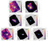 |
Fig. 3 Integrated intensity maps of atomic and molecular lines detected with JWST/MIRI MRS. In color, the line-integrated intensity is shown in a log-scale. The JWST/MIRI 5.2 μm continuum is presented as blue contours with contour levels at 5, 10, 15, 20, and 25 × σcont,5μm. The two mm sources are indicated by green squares and several shock positions are highlighted by green crosses. The angular resolution of the JWST/MIRI continuum and the line data are shown in the bottom left and right corners, respectively. In the top left panel, the bipolar outflows are indicated by red and blue dashed arrows. The shock locations (Sect. 3.2) and continuum sources are labeled in the top right and center left panel, respectively. In the [Ne II] and [Ne III] panels, the dash-dotted gray circles show the aperture (0.″9) in which the flux density was derived (Sect. 4). |
3.2.5 Millimeter lines
The integrated intensity maps of the mm lines are shown in Fig. 4. The bipolar outflows can also be partially revealed in the mm line data. A common shock tracer in the mm regime is SiO, with silicon (Si) being sputtered off the grains and forming SiO in the gas phase (e.g., Schilke et al. 1997). The SiO emission peak is toward the northern part, close to the shocked positions S2 and S3 that are also bright in H2 and [S I]. 13CS also shows an elongated structure toward the northern part. SO, H13CO+, and H2CO show bright emission toward mmA1, but are also enhanced toward the northern direction toward S2 and S3. The north-south outflow (II) thus has a rich molecular component.
In SiO, a large-scale outflow (I) is seen from the northwest to the southeast, which is also revealed by the CORE 1 mm data (Cesaroni et al. 2019). This large-scale northwest-southeast molecular outflow (I) is also faintly seen in SO, H2CO, and CH3OH and is also detected in H2 by JWST/MIRI (Fig. 2). The S-shaped morphology of the outflow, most evident in SiO, suggests a precessing jet due to binary interaction (e.g., Eisloffel et al. 1996; Fendt & Zinnecker 1998; Brogan et al. 2009; Sheikhnezami & Fendt 2015).
OCS shows very compact emission toward mmA1. HC3N shows extended emission with many filamentary structures, hinting at not only outflowing but most likely also inflowing gas, and peaks toward mmA1. CH3CN emission is strong around mmA1 and A/mmA2. Interestingly, CH3OH emission significantly drops toward the locations of the MIR-bright sources A/mmA2 and B.
mmB does not show significant emission peaks in any of the NOEMA emission maps, except for CH3OH emission. As all remaining detected continuum sources (mmA1, A/mmA2, and B) show protostellar activity through outflows and ionized gas, mmB is likely to be less evolved or less massive, although it cannot be completely ruled out that the H2 and [S I] emission toward S1 could be an outflow originating from mmB, which is directed along the line of sight.
Shocks near the protostars are caused by the emerging outflows and are seen in SiO emission, but also in sulfur-bearing species, such as atomic sulfur, SO, and 13CS. However, OCS only emits strongly toward the source mmA1, suggesting that it may be related to ice sublimation instead of shock chemistry. For SO, both high-temperature gas-phase chemistry close to the protostar and shock chemistry in the outflow (II) seem to be relevant to explain the spatial distribution. The entire region is embedded in a filamentary structure seen in HC3N, where most of these converge toward the central dense core. This suggests that, even though there exist at least three outflows seen in H2 emission by MIRI (I, II, and III, Fig. 2), they have so far had only little impact on the envelope in which the protostars are embedded. Thus, further star formation activity could still be possible in the central dense core of IRAS 23385 toward the dense mm source mmB, which currently does not show any signatures of active star formation.
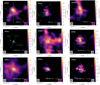 |
Fig. 4 Integrated intensity maps of molecular lines detected with NOEMA plotted over the same area as the JWST data in Figs. 2 and 3. In color, the line-integrated intensity is shown. The JWST/MIRI 5.2 μm continuum is presented as blue contours with contour levels at 5, 10, 15, 20, and 25 × σcont,5μm. The two mm sources are indicated by green squares and several shock positions are highlighted by green crosses. The synthesized beam of the NOEMA continuum and the line data are shown in the bottom left and right corners, respectively. In the top left panel, the bipolar outflows are indicated by red and blue dashed arrows (Beuther et al. 2023). The shock locations (Sect. 3.2) and continuum sources are labeled in the top central and center left panels, respectively. |
3.3 Molecular hydrogen excitation diagram analysis
The JWST/MIRI MRS spectral range covers multiple transitions of the pure rotational 0−0 state of H2 (Table 1) and the H2 column density N(H2) and rotational temperature Trot can be estimated based on the excitation diagram analysis (e.g., Neufeld et al. 2009). The lowest H2 transitions are excited through collisions (e.g., Black & van Dishoeck 1987), while higher rotational levels and vibrational states can be excited through UV pumping. The warm component linked to the collisions is therefore a realistic tracer of the underlying gas temperature, while for any hotter component, the estimated rotation temperature may not correspond to a physical property. As the angular resolution varies from 0.″2 to 0.″8 for 5 μm to 28 μm along the full MIRI spectral range, we smooth the S(7) to S(1) transitions to a common resolution of 0.″7 that corresponds to the angular resolution of the S(1) transition and regrid the remaining lines to the same spatial grid as the H2 S(1) data. Spectral binning is not performed. This allows us to carry out a pixel-by-pixel excitation diagram analysis and to obtain a complete N(H2) and Trot map, because the H2 transitions are detected within the entire FoV.
To provide reliable results, it is crucial to correct for extinction along the line of sight. We use an extinction curve derived by McClure (2009) that is valid between K-band (2.2 μm) magnitudes AK of 1 mag and 7 mag. As the extinction toward the central dense core is expected to be high (Molinari et al. 1998b), we assume a K-band extinction of AK = 7 mag in the entire FoV, which roughly corresponds to a visual extinction of ≈50 mag. We also tested lower values of AK, but found that the integrated intensity of the S(3) transition that is located within the broad 10 μm silicon-absorption feature (Beuther et al. 2023) is significantly decreased compared to the transitions outside of the absorption feature for these lower values of AK.
As a first step, in each spatial pixel, the seven H2 transitions using the extinction-corrected data were fitted by a 1D Gaussian and from the integral of the Gaussian fit the integrated intensity of each transition was computed. Example spectra and Gaussian fits of the seven transitions taken from the position of source mmA1 and source B are presented in Fig. A.1. The integrated line intensities toward all four continuum sources (Table 3) and four shock positions (S1, S2, S3, and S4) are summarized in Table A.1.
In general, the lines are barely resolved at the spectral resolution of MIRI. The uncertainty in the absolute flux calibration of the MIRI MRS instrument is only on the order of a few percent (Argyriou et al. 2023). A much higher uncertainty in the calculation of the line-integrated intensities arises from the extinction correction: we assume AK = 7 mag (AV = 54 mag) in the entire FoV, while there may be spatial differences. For comparison, in Table A.1 we also present the extinction-corrected integrated line intensities calculated with AK = 5 mag (AV = 39 mag) and AK = 3 mag (AV = 23 mag). A value of AV = 30-40 mag is estimated from the 9.7 μm silicate absorption feature (Rocha et al., in prep.), whereas previous studies suggested even higher extinction values of AV = 200 mag (Molinari et al. 1998b). Given the high column densities toward the region, AK = 5–7 mag should be a reliable estimate of the extinction. The line-integrated line intensities vary by a factor of between 2 and 3 within this K-band extinction range (Table A.1). We therefore assume in the following that the observed line-integrated intensities are uncertain by a factor of two.
Moreover, only transitions with a peak intensity of 50 MJy sr−1 (which is above the noise in the nonextinction-corrected data) and above are further considered (Table 1). With this threshold, we exclude areas with faint H2 emission in the higher excited lines where the excitation diagram analysis would provide unreliable results. As an additional constraint, a fit to the excitation diagram is only performed when five or more transitions are detected in a spatial pixel above the threshold, as otherwise a two-component fit would not provide reliable results.
The excitation diagram analysis is performed using the pdrtpy3 Python package. Typically, it is found that the observed H2 transitions are best described by two rotational temperature components, which we refer to as Twarm and Thot in the following. The observed line-integrated intensities are converted into upper-state column densities normalized by their statistical weight, Nu/gu. The H2 rotation temperature and column density can be estimated by plotting the logarithm of Nu/gu, as a function of the upper-state energy level, Eu/kB, and fitting the observed data points with a straight line for each component. The column density, log N, is proportional to the y-intercept and the slope is proportional to −1/T. We assume that all H2 transitions are optically thin (which is valid even for N(H2) > 1023 cm−2, Bitner et al. 2008).
Examples of the excitation diagram toward the sources mmA1 and B are shown in Fig. 5. The fit results obtained from pdrtpy for the warm and hot component toward all four continuum sources (Table 3) and four shock positions (S1, S2, S3, and S4) are summarized in Table A.2. Considering all positions in the map, the uncertainties for the estimated temperature are between 10 and 30%, while for the column densities the uncertainties are on the order of a factor of 0.5−3. In absolute numbers, the median uncertainties are log ΔNwarm = cm−2, log ΔNhot = 0.6 cm−2, ΔTwarm = 43 K, and ΔThot = 270 K.
The spectral line extraction and excitation diagram analysis toward the mmA1 and B sources shown in Figs. A.1 and 5, respectively, reveal bright line emission in all transitions of H2. The excitation diagram shows the necessity to fit the data with two temperature components. The warm and hot temperature components toward mmA1 are ≈400 and ≈1400 K, respectively. The total column density, considering the contribution from both temperature components, is Nwarm+hot ≈ 5 × 1023 cm−2. Toward source B we find a higher column density but lower temperature. This could be attributed to the fact that the less excited H2 lines may become optically thick toward the MIR sources; this possibility is further discussed in Sect. 4.
In Table A.2, we also present excitation diagram fitting results, with AK = 5 mag and AK = 3 mag assumed in the calculation of the extinction-corrected line-integrated intensities (Table A.1). As expected, the estimated column densities are higher when the extinction is higher. However, given the high uncertainties, the differences are not significant. There is an effect on the derived temperatures. While the temperature of the hot component does not significantly change, the temperature of the warm component does show some differences, although these cannot be considered significant given the high uncertainties. This is due to the fact that the S(3) line of H2 lies in the silicate absorption feature and thus suffers from a higher extinction Αλ compared to the remaining lines. As this line lies at the border of the two components in the excitation diagram (Fig. 5), this data point does influence the fitted slope and thus the estimated temperature.
The complete temperature and column density maps of the warm and hot components are presented in Fig. 6, and in Sect. 4 we compare the results with rotation temperature estimates based on the cold gas traced by the NOEMA data. One caveat, mentioned above, is that the excitation diagram analysis assumes that the H2 lines are optically thin, which may not be the case, especially toward the positions of the MIR sources A/mmA2 and B.
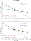 |
Fig. 5 Example of the H2 excitation diagram analysis with pdrtpy of source mmA1 (top) and source B (bottom). The observed data are shown in black and the two-component fit is shown by red and blue dots, which correspond to the warm and hot component, respectively, and the total fit is indicated by a green line. |
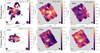 |
Fig. 6 Temperature and H2 column density of the gas components in IRAS 23385 derived using CH3CN and H2 as a diagnostic tool (Sects. 3.3 and 3.4). In the top and bottom panels, the rotation temperature and H2 column density map, respectively, of the cold (left), warm (center), and hot (right) components are shown in color. The angular resolution of the line data is indicated by a purple ellipse in the bottom right corner. The JWST/MIRI 5.2 μm continuum is presented by blue contours with contour levels at 5, 10, 15, 20, and 25 × σcont,5μm and the angular resolution is highlighted by a black ellipse in the bottom left corner. The NOEMA 3 mm continuum (top and bottom left panels) is highlighted by gray contours with levels at 5, 10, 20, 40, and 80 × σcont,3mm and the synthesized beam is highlighted by a gray ellipse in the bottom left corner. All continuum sources are labeled in green in the bottom left panel and the mm continuum sources are marked by green squares. Several shock positions are indicated by green crosses (Sect. 3.2). |
3.4 Methyl cyanide line modeling
Molecular emission at mm wavelengths can be used to probe the temperature of the cold molecular gas. In Gieser et al. (2021), the temperature of the cold gas component in the CORE regions, including IRAS 23385, is estimated using H2CO and CH3CN emission lines. Unfortunately, the H2CO lines are optically thick toward the center of IRAS 23385, causing XCLASS to converge to unrealistically high temperatures >200 K. However, this highlights again that toward the central core, the densities and extinction must be high. For CH3CN, the temperature toward mmA1 is estimated to be 100 K (Cesaroni et al. 2019; Gieser et al. 2021); however, the transitions of the J = 12–11 K-ladder at 1 mm have high upper state energies and therefore the emission is compact around mmA1 and barely resolved. With the complementary 3 mm CORE+ observations of the CH3CN J = 5–4 K-ladder, the temperature of more extended colder gas can be investigated (Table 2).
We model the rotational transitions of the CH3CN J = 5–4 K-ladder with XCLASS. With XCLASS, the 1D radiative transfer equation is solved assuming local thermal equilibrium (LTE) conditions. The fit parameters are source size θsource, rotation temperature Trot, column density N(CH3CN), line width Δν, and velocity offset voff. In total, we model four transitions of CH3CN (J = 5−4 and K = 0, 1, 2, 3, Table 2) and from the best-fit, the rotation temperature can be estimated. As these CH3CN transitions have upper state energy levels < 100 K compared to the JWST/MIRI H2 transitions with >1000 K, we refer to this temperature component as the cold component, Tcold. In each spatial pixel, the CH3CN spectrum is modeled with XCLASS if the peak brightness temperature is higher than a threshold of 0.7 K (corresponding to ≈3−4σline, Table 2).
As an example, the observed spectrum and best-fit model derived with XCLASS is shown in Fig. A.2 toward the position of mmA1. The derived rotation temperature, column density, and line width of CH3CN are 46 K, × 1013 cm−2, and 3.7 km s−1, respectively. The full temperature map is presented in Fig. 6 and is discussed and compared to the temperature estimated from H2 in Sect. 4.
Using the CH3CN temperature and the 3 mm continuum data, we can also estimate the H2 column density of the cold component, under the assumption that the 3 mm continuum stems from optically thin dust emission, and also that the gas and dust temperatures are coupled. The 3 mm continuum optical depth can be calculated according to
 (1)
(1)
where Ipix,3mm is the 3 mm intensity in a pixel, converted from Jy beam−1 to Jy pixel−1 considering the beam area Ω = π/(4ln2)θmajθmin and the area covered by one pixel (0.25″)2, and Bv(Tcold) is the Planck function. We find that τcont,3mm < 0.02 in the entire map. Thus, the 3 mm continuum emission stems from optically thin dust emission.
Using the 3 mm continuum data, which has a similar angular resolution, and the CH3CN temperature map, the H2 column density of the cold gas can be derived (Hildebrand 1983):
 (2)
(2)
We assume a gas-to-dust mass ratio of γ = 150 (see Beuther et al. 2018), a dust opacity of κν = 0 17 cm2 g−1 (Table 1 in Ossenkopf & Henning 1994, extrapolated from 1.3 mm, and assuming thin icy mantles at a gas density of 106 cm−3), a mean molecular weight of μ = 2.8, and mH is the mass of a hydrogen atom. The flux calibration of NOEMA is expected to be accurate to a 10% level at 3 mm4. The temperatures estimated with CH3CN in XCLASS have uncertainties on the order of 30% (Gieser et al. 2021). The biggest uncertainty when estimating Ncold lies in the gas-to-dust mass ratio γ and the dust opacity κν. It can therefore be estimated that the calculated Ncold values can be uncertain up to a factor of 2–4 (Beuther et al. 2018). The results for Tcold, Mcold, and Ncold(H2) are presented in Fig. 6 and are discussed in Sect. 4.
4 Discussion
The JWST/MIRI MRS observations of IRAS 23385 reveal exciting new insights into energetic processes during the formation of stars. Multiple outflows (I, II, and III, Fig. 2) can be identified, one of which shows, in addition to H2 and [S I] emission, enhanced emission from [Fe II], [Ni II], and [Ne II]. The outflows are also associated with cold molecular gas traced by mm lines. Here, we focus on a few main points based on the analysis (Sect. 3) and discuss in detail the different gas components, the outflow properties, and the spatial emission and intensity ratio of [Ne II] and [Ne III].
4.1 Gas components toward the central dense core
A comparison of the warm and hot gas traced by H2 in the JWST/MIRI observations (Sect. 3.3) and the cold gas traced by CH3CN and the 3 mm continuum in the NOEMA observations (Sect. 3.4) is presented in Fig. 6. The top and bottom panels show the H2 rotation temperature and column density, respectively, of the cold (left), warm (center), and hot component (right). To our knowledge, this is the first time that spatially resolved maps of the cold, warm, and hot components have been obtained in a high-mass cluster-forming region. The cold component consists of dense (1023–1024 cm−2) and cold (10–60 K) gas. Interestingly, we derive similar column densities for the warm component, but these are spatially different, because the H2 lines trace shocked and heated gas due to the outflows, while the mm line and continuum trace the cold envelope. The temperature of the warm component ranges between 200 and 400 K.
Comparing the temperature and column density, we find that these properties are anti-correlated, such that the temperature is lower toward the high column densities compared to the lower-column-density regions. This suggests that toward the dense shocks, the lower H2 lines could become optically thick and we only trace outer layers toward these shock positions. In the hot component, the column densities are about two orders of magnitude lower, of namely Nhot ≈ 1022 cm−2, compared to the cold and warm component and the temperatures are 1000–1800 K.
It is interesting to consider how these temperatures and column densities compare with those found in nearby low-mass regions for which more extensive studies are available in the literature. Taking as an example the L1157 Class 0 protostar (L = L⊙, Froebrich 2005), Di Francesco et al. (2020) studied the cold material using Herschel observations and find dust temperatures of 10–18 K and column densities of up to 2 × 1022 cm−2. Nisini et al. (2010) created temperature and H2 column density maps of the L1157 outflow and also find that the H2 line fluxes are best described by two temperature components, with 300–400 K and 1100–1400 K, respectively. These results are similar to the temperatures derived in the IRAS 23385 region (Fig. 6); however, the H2 column density map derived by Nisini et al. (2010) is about four orders of magnitude lower, which is expected in less massive outflows driven by low-mass protostars. Compared to previous IR studies toward HMSFRs, with JWST we are for the first time able to probe high-column density regions (>1023 cm−2) thanks to the higher angular resolution. The temperature in IRAS 23385 is also similar to low-mass protostars in NGC 1333 (Dionatos et al. 2020). In the regime of high-mass protostars, van den Ancker et al. (2000) find temperatures of the warm component of 500 and 730 K for the HMSFR S106 and Cep A, respectively. In the Orion OMC-1 outflow, Rosenthal et al. (2000) find that the bulk (≈72%) of the warm gas has a temperature of ≈630 K.
A system that is comparable to IRAS 23385 is IRAS 20126+4104 (d = 1.7 kpc, Cesaroni et al. 1997), which has a central protostar of similar mass (7 M⊙) and luminosity (104 L⊙). Jet precession in this source also hints at underlying multiplicity (e.g., Cesaroni et al. 2005; Caratti o Garatti et al. 2008). Using higher excited transitions of H2 in the NIR, a high temperature component at 2000 K is derived by these latter authors, while a warm component is also found at 500 K. Additional observations in the NIR, for example with the Near-Infrared Spectrograph (NIRSpec) instrument of JWST, are required in order to investigate the presence of components in IRAS 23385 of potentially even higher temperature.
Toward IRAS 23385, the highest mass protostar is estimated to be 9 M⊙ (Cesaroni et al. 2019), which is at the lower end of what is considered as a “high-mass” star, and therefore it is expected that more massive protostars can heat up the environment to even higher temperatures through powerful outflows and expanding UCHII regions. The fact that a cold component such as that traced by the NOEMA mm observations still exists toward the central dense core suggests that star formation can efficiently occur in shielded dense gas. While outflows seem to impact the surrounding envelope through shocks and heating of the material, the feedback is not (yet) strong enough to completely dissipate the central dense core as outflows are collimated.
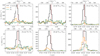 |
Fig. 7 JWST/MIRI MRS spectra of atomic line emission. In each panel, the spectra presented were extracted from the positions at the MIR source A/mmA2 (black, Table 3) and two shock locations (orange: S1 and green: S3, see Fig. 3). The bottom and top x-axes show the observed wavelength and velocity, respectively. The red vertical line indicates the wavelength of the line at a source velocity of −50.2 km s−1. |
4.2 Composition of the outflows and evolutionary stage of the continuum sources
The northeast-southwest outflow III (Fig. 2) is not only seen in H2 and [S I] emission knots, but these knots are also bright in [Fe II] and [Ni II] emission (Fig. 3). Dionatos et al. (2014) find [Fe II] and [Ne II] to trace the FUV irradiation on the disk surface and on the walls of the outflow cavity and Caratti o Garatti et al. (2015) also find that [Fe II] and H2 knots can be co-spatial. Toward the position of the source A/mmA2, we detect emission from ionized atoms from [Fe II], [Ni II], [Ne II], [Ne III], and [Ar II] (Fig. 3). This suggests that this protostar is the most evolved, with strong UV and X-ray radiation. The ionization energies are 7.6 eV (Ni), 7.9 eV (Fe), 15.8 eV (Ar), and 21.6 eV (Ne). In Fig. 7, example spectra of the atomic transitions extracted from the positions of the continuum source A/mmA2 and the shock positions S1 and S3 are shown. The [S I] line peaks at the source velocity toward source A/mmA2 and shock position S1. The shock position S3 caused by the redshifted part of outflow II is also redshifted, as expected. If detected, [Ni II], [Ar II], and [Fe II] lines are blueshifted compared to the source velocity tracing the blueshifted outflow components. The [Ne II] and [Ne III] lines are further discussed in Sect. 4.3.
Rosenthal et al. (2000) studied the MIR spectrum of one of the brightest H2 shock positions of the Orion OMC-1 outflow. In comparison with the IRAS 23385 outflows, these authors find emission from doubly or triply ionized fine structure lines of [Fe III], [S III], [P III], [S IV], and [Ar III], while in IRAS 23385 only [Ne III] is detected (the emission of this line is further discussed in the following). This suggests that the protostars and their outflows in IRAS 23385 are not energetic enough to produce and excite the doubly or higher ionized transitions.
We do not detect MIR continuum emission toward the mm continuum peak source mmA1. Either the extinction is too high toward the location of this source, for example due to the geometry or high density, or the protostar itself is at an earlier evolutionary phase compared to the MIR-bright sources A/mmA2 and B. However, we could expect this source to become bright at the longer wavelengths within the MIRI coverage, which is not the case. The bipolar outflow (II) in the north-south direction only consists of molecules and neutral atomic lines (see Fig. 7 for the atomic line emission at the shock position S1). The fact that CH3CN and OCS emission is detected toward the location of mmA1 suggests that the central protostar is currently heating up the surrounding material, creating a hot core region where ices sublimate from the grains. The high density may currently still prevent energetic UV and X-ray radiation and also the MIR radiation of the protostar itself from escaping far from the protostar, with it remaining undetected in the MIR.
The source mmB does not show any signatures of star-forming activity. Moreover, the CH3OH emission detected toward the location of mmB may be shocked gas originating from the northeast-southwest outflow (III). However, it may not be a coincidence that mmB is along this outflow direction, as it may be cold material that was swept up by outflow (III).
Tychoniec et al. (2021) provide an overview of the molecular lines that trace different physical entities surrounding low-mass Class 0 and I protostars; for example, the hot core region, outflows, UV-irradiated cavity walls, jets, disks, and the surrounding envelope (see their Fig. 11 and Table 2). All molecular lines at mm wavelengths presented in this work (Fig. 4) - except for HC3N - are covered by their overview. We find a similar spatial distribution in IRAS 23385, though due to the large distance we are not able to resolve a potential disk or differentiate between the outflow and cavity walls. Interestingly, we do not find strong emission by complex organic molecules (COMs), except for CH3OH and CH3CN. The observed CH3OH emission traces the outflow (I); it is nonthermally desorbed and likely sputtered as observed in Perotti et al. (2021). Given that the temperature of the cold component is ≈60 K, the COMs may still mostly reside in ices on the dust grains. The composition of the MIRI MRS ice absorption spectra could reveal the presence of COMs in the ices and will be presented in Rocha et al. (in prep.). Early JWST observations toward low-mass protostars and their envelopes have already revealed a variety of different ice species (Yang et al. 2022; McClure et al. 2023).
For both outflows III and II (Fig. 2), the atomic sulfur is co-spatial with H2 knots caused by shocks due to the outflow (Fig. 3). This suggests that sulfur is being released by C-type shocks (similar to outflows of Class 0 protostars, Anderson et al. 2013). As the observed [S I] line at 25.2 μm has a large critical density (105 cm−3, Hollenbach & McKee 1989), it will be readily detected in high-density shocked gas. Its abundance can be enhanced with sputtering of the grains in shocks.
Shocks in star-forming regions can occur through various processes; for example, cloud-cloud collisions, jets and molecular outflows, stellar winds, and expanding H II regions. In C-type shocks, the maximum temperature is 2000–3000 K and shock velocities are <40 km s−1, which is too low to destroy molecules, while temperatures can reach 105 K in J-type shocks, with increased fine structure emission from atoms such as Fe, Mg, and Si that sputter off the grains, and shock velocities that are typically higher than 40 km s−1 (Hollenbach & McKee 1989; van Dishoeck 2004). With the relatively low spectral resolution of JWST/MIRI MRS (R ≈ 3700−1400), it is difficult to estimate the shock velocities; however, the presence of [Fe II] (velocity-resolved maps from −185 to 120 km s−1 are presented in Beuther et al. 2023, their Fig. 6) and [Ni II] in the northeast-southwest outflow (III) suggests that there could be a contribution from J-type shocks, while for the remaining two outflows (II and I) only enhanced emission of H2 and [S I] is detected, and ionized atomic fine structure lines are absent toward these outflow directions.
4.3 PDRs versus shocks: The case of [Ne II] and [Ne III]
Previous ISO observations suggested that [Ne II] could be tracing dissociative (J-type) shocks (van Dishoeck 2004). With the low angular resolution of these older data, often multiple physical entities are covered; for example, H II regions, photon-dominated and photon-dissociation regions (PDRs), and outflows (e.g., in Orion IRc2 van Dishoeck et al. 1998). In addition, due to low filling factors toward distant HMSFRs, such lines were often not detected. With JWST/MIRI MRS, we are able to resolve individual components. Indeed, both shocks and PDRs can contribute to many of the lines observed in this work.
The spatial morphology of the [Ne II] line (Fig. 3) reveals extended emission within the full MIRI FoV, and is also detected toward the east at the arc-like structure, which is a PDR illuminated by the nearby UCH II region. In PDRs, the radiation field is dominated by FUV photons (6–13.6 eV) (e.g., Hollenbach & Tielens 1999). PDRs show emission by MIR H2 transitions, as well as neutral and singly ionized atomic fine structure lines (van Dishoeck 2004, and references within). In the case of the IRAS 23385 PDR, we detect emission of H2 and [Ne II] in the arc, highlighting the impact of the clustered mode of high-mass star formation, including photons with energies of >13.6eV, which can ionize neon.
The [Ne II] transition also traces both outflows and the inner disk toward low-mass protostars, where these regions can be sufficiently resolved (Sacco et al. 2012). These latter authors find that the [Ne II] emission is slightly blueshifted (2–12 km s−1) and argue that it may originate from a disk wind. Glassgold et al. (2007) suggest that the emission could stem from the disk that is irradiated by stellar X-rays. [Ne II] is commonly detected in Class II disks (Pascucci et al. 2023). While most atomic fine structure lines are indeed blueshifted by 50–100 km s−1 with respect to the source velocity, the [Ne II] and [Ne III] lines toward the position of source A/mmA2 are not blueshifted but are more centered on the source velocity (Fig. 7); therefore, the emission at source A/mmA2 could either stem from the protostar itself or a disk wind.
Considering the [Ne II] and [Ne III] peak toward the west of source A/mmA2 (Fig. 3), a disk wind is unlikely to explain the emission since it is ≈5000 au offset from the MIR source. Another explanation could be that we are tracing the UV and X-ray irradiated cavity of the large-scale northwest-southeast outflow (I) launched from source B. However, the emission is not perfectly aligned with that direction. The fact that most emission lines toward source A/mmA2 shown in Fig. 7 are blueshifted compared to the source velocity, while [Ne II] and [Ne III] peak at the source velocity, suggests that [Ne II] and [Ne III] are tracing a region closer to the protostar. The origin of the [Ne II], [Ne III], and faint [Ar II] emission to the west of source A/mmA2 (Fig. 3) remains unclear.
High-mass (proto)stars have enough UV intensity to ionize [Ne II] and [Ne III]. To estimate the line-integrated flux density of both [Ne II] and [Ne III] transitions, we perform aperture photometry with an aperture of 0.″9 toward both [Ne III] peak positions (highlighted by gray dash-dotted circles in Fig. 3). Toward source A/mmA2, the line-integrated flux density is 3.1 mJy for [Ne II] and 0.23 mJy for [Ne III], while toward the western position these values are 2.6 mJy and 0.19 mJy, respectively. While the flux density is higher at the position of source A/mmA2, the [Ne II]/[Ne III] flux density ratio at both positions is similar (13 and 14), suggesting that even at a projected distance of 5 000 au, the X-ray and UV radiation from the protostar can efficiently funnel along the outflow. Simpson et al. (2012) find [Ne II]/[Ne III] ratios of between 17 and 125 in a sample of massive protostars in the G333.2–0.4 giant molecular cloud and Rosenthal et al. (2000) find a ratio of 0.95 toward the brightest outflow knot in the Orion OMC-1 outflow. van Dishoeck et al. (1998) derived a ratio of 1.4 toward the Orion IRc2 source that causes this outflow and a ratio of 1.3–1.9 in the Orion PDR. Güdel et al. (2010) find a higher [Ne II] luminosity in sources associated with jets compared to those without, which would be consistent with our high ratio. These latter authors find a weak correlation with X-ray luminosity. When the full sample of the JOYS targets is observed, a statistical analysis of such properties can be conducted from low- to high-mass protostars and contributions from jets versus UV and/or X-rays can be disentangled.
5 Conclusions
In this study, we compare the MIR properties of the warm gas in IRAS 23385 - traced by JWST/MIRI MRS observations that are part of the JOYS project - with the cold material traced by NOEMA observations at mm wavelengths. In total, four continuum sources are resolved that are all embedded within the dense cold envelope. Two sources are MIR bright, while the two bright mm cores remain undetected in the MIRI range between 5 and 28 μm. The spatial morphology of the atomic and molecular lines is investigated using integrated intensity maps. The gas temperature and column density of different components are estimated using H2 MIR and CH3CN mm line emission and 3 mm continuum emission. Our conclusions are summarized as follows:
Combining the JWST/MIRI MRS and NOEMA observations allows us to disentangle several gas components, consisting of cold (<100 K), warm (200–400 K), and hot (≥1 000 K) material traced by CH3CN and H2 lines. While the warm and hot component - which is mostly caused by heated and/or shocked gas in the outflows - is extended, there is still a significant amount of cold material that allows for star formation to proceed. This is also highlighted by the H2 column densities of the cold and warm components that are both on the order of 1024 cm−2. The column density of the hot component is, in contrast, significantly lower, at approximately 1022 cm−2.
The H2 0–0 S(1) to S(7) transitions reveal C-type shocked and extended warm gas originating from multiple bipolar outflows (I, II, and III). These are also evident in the atomic sulfur line [S I], stressing the importance of sulfur being released from the grains due to shocks. The outflows and their cavities can also be seen in many molecular lines at mm wavelengths (SiO, SO, 13CS, H13CO+, H2CO, CH3OH).
An energetic outflow (III) emerges probably from source A/mmA2, where the blueshifted outflow reveals emission knots by [Fe II] and [Ni II]. Thus, the outflow seems to have undergone multiple outbursts in the past causing dissociative J-type shocks.
The MIR source A/mmA2 also shows enhanced emission from [Fe II], [Ni II], [Ne II], [Ne III], and [Ar II] toward the central location of the protostar. While the emission is blueshifted by 50–100 km s−1 compared to the source velocity for most of these species, the emission from [Ne II] and [Ne III] peaks at the source velocity. This suggests that, in these cases, not only may the outflow cause the ionization and excitation of the line emission, but, for example, a disk wind or the disk atmosphere itself or an X-ray irradiated cavity may be the cause. However, the angular and spectral resolution are not sufficient to differentiate between these possibilities.
The [Ne II] emission is extended within the full MIRI FoV and also traces bright emission toward the edges of the MIRI FoV, a PDR region caused by the nearby UCHII regions (Fig. 1).
To fully understand the clustered properties of high-mass star formation, it is important to conduct a multiwavelength study tracing both the warm and the cold gas properties. With JWST, we now have a new and unprecedented view of the IR properties and diagnostics of protostars and their environments at high angular resolution and sensitivity.
Acknowledgements
This work is based on observations made with the NASA/ESA/CSA James Webb Space Telescope. The data were obtained from the Mikulski Archive for Space Telescopes at the Space Telescope Science Institute, which is operated by the Association of Universities for Research in Astronomy, Inc., under NASA contract NAS 5-03127 for JWST. These observations are associated with program #1290. The following National and International Funding Agencies funded and supported the MIRI development: NASA; ESA; Belgian Science Policy Office (BELSPO); Centre Nationale d’Etudes Spatiales (CNES); Danish National Space Centre; Deutsches Zentrum fur Luftund Raumfahrt (DLR); Enterprise Ireland; Ministerio De Economiá y Competividad; Netherlands Research School for Astronomy (NOVA); Netherlands Organisation for Scientific Research (NWO); Science and Technology Facilities Council; Swiss Space Office; Swedish National Space Agency; and UK Space Agency. This work is based on observations carried out under project number L14AB and W20AV with the IRAM NOEMA Interferometer and the 30 m telescope. IRAM is supported by INSU/CNRS (France), MPG (Germany) and IGN (Spain). H.B. acknowledges support from the Deutsche Forschungsgemeinschaft in the Collaborative Research Center (SFB 881) “The Milky Way System” (subproject B1). E.D., M.G., L.F., K.S., W.R. and H.L. acknowledge support from ERC Advanced grant 101019751 MOLDISK, TOP-1 grant 614.001.751 from the Dutch Research Council (NWO), the Netherlands Research School for Astronomy (NOVA), the Danish National Research Foundation through the Center of Excellence “InterCat” (DNRF150), and DFG-grant 325594231, FOR 2634/2. P.J.K. acknowledges financial support from the Science Foundation Ireland/Irish Research Council Pathway programme under Grant Number 21/PATH-S/9360. A.C.G. has been supported by PRIN-INAF MAIN-STREAM 2017 “Proto-planetary disks seen through the eyes of new-generation instruments” and from PRIN-INAF 2019 “Spectroscopically tracing the disk dispersal evolution (STRADE)”. K.J. acknowledges the support from the Swedish National Space Agency (SNSA). T.H. acknowledges support from the European Research Council under the Horizon 2020 Framework Program via the ERC Advanced Grant “Origins” 83 24 28. T.P.R. acknowledges support from ERC grant 743029 EASY.
Appendix A Fit examples and results
In Sect. 3.3 the H2 0–0 S(1) to S(7) transitions covered by JWST/MIRI are used in order to estimate the temperature of the warmer gas. All lines are smoothed to a common angular resolution of 0.″7 and spatially regridded to the S(l) line data. In each spatial pixel, the spectra are extracted and fitted by a Gaussian + constant component to include the continuum emission. The line-integrated intensities are listed in Table A.1 for all continuum sources and shock positions assuming AK = 7 mag in the calculation of the extinction-corrected line-integrated intensities. For comparison, we also show the results for AK = 5 mag and AK = 3 mag. Figure A.1 shows the observed spectra and corresponding Gaussian fit toward the positions of source mmA1 (top panel) and source Β (bottom panel). The spectra are corrected for extinction using the extinction curve derived by McClure (2009).
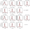 |
Fig. A.1 Examples of the observed and extinction-corrected H2 lines (black) and Gaussian fit (red line) of source mmAl (top) and source Β (bottom). The vertical gray line indicates the wavelength of each transition. |
The line-integrated intensities of the Gaussian fits are converted to upper-state column densities divided by the statistical weight and when plotted against the upper energy level, the H2 rotation temperature and column density can be estimated from the slope and intercept, respectively. Examples of the H2 excitation diagrams are shown in Fig. 5 for sources mmA1 and B. As is often the case for star-forming regions, the profile is best described by two temperature components, which we refer to as the “warm” and “hot” component in contrast to the “cold” component traced by the NOEMA data. The fit results for the warm and hot component are summarized in Table A.2 for all continuum sources and shock positions. For comparison, we also present the results using extinction values of AK = 5 mag and AK = 3 mag. There are no significant differences between the derived column densities. A small effect is seen for the temperatures given that the S (3) transition that lies in the silicate absorption feature influences the two fitted slopes.
The temperature of the cold component is estimated using CH3CN line emission covered by the CORE+ project. In each spatial pixel, the CH3CN J = 5−4 K-ladder is modeled using XCLASS (Möller et al. 2017). An example toward the location of the mmAl source is shown in Fig. A.2. In these examples, we trace for source mmAl temperature components at 50 K, 400 K, and 1400 Κ using the H2 and CH3CN lines as thermometers.
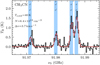 |
Fig. A.2 Example of CH3CN line modeling with XCLASS. The observed spectrum toward mmA1 is shown in black, and the best-fit model derived by XCLASS in red. The modeled transitions of CH3CN (Table 2) are indicated by blue vertical bars. |
References
- Ahmadi, A., Beuther, H., Mottram, J. C., et al. 2018, A & A, 618, A46 [NASA ADS] [CrossRef] [EDP Sciences] [Google Scholar]
- Ahmadi, A., Beuther, H., Bosco, F., et al. 2023, A & A, 677, A171 [CrossRef] [EDP Sciences] [Google Scholar]
- Anderson, D. E., Bergin, E. A., Maret, S., & Wakelam, V. 2013, ApJ, 779, 141 [Google Scholar]
- Argyriou, I., Glasse, A., Law, D. R., et al. 2023, A & A, 675, A111 [NASA ADS] [CrossRef] [EDP Sciences] [Google Scholar]
- Beuther, H., Mottram, J. C., Ahmadi, A., et al. 2018, A & A, 617, A100 [NASA ADS] [CrossRef] [EDP Sciences] [Google Scholar]
- Beuther, H., van Dishoeck, E. F., Tychoniec, L., et al. 2023, A & A, 673, A121 [NASA ADS] [CrossRef] [EDP Sciences] [Google Scholar]
- Bitner, M. A., Richter, M. J., Lacy, J. H., et al. 2008, ApJ, 688, 1326 [NASA ADS] [CrossRef] [Google Scholar]
- Black, J. H., & van Dishoeck, E. F. 1987, ApJ, 322, 412 [Google Scholar]
- Brogan, C. L., Hunter, T. R., Cyganowski, C. J., et al. 2009, ApJ, 707, 1 [CrossRef] [Google Scholar]
- Caratti o Garatti, A., Froebrich, D., Eislöffel, J., Giannini, T., & Nisini, B. 2008, A & A, 485, 137 [CrossRef] [EDP Sciences] [Google Scholar]
- Caratti o Garatti, A., Stecklum, B., Linz, H., Garcia Lopez, R., & Sanna, A. 2015, A & A, 573, A82 [CrossRef] [EDP Sciences] [Google Scholar]
- Cesaroni, R., Felli, M., Testi, L., Walmsley, C. M., & Olmi, L. 1997, A & A, 325, 725 [NASA ADS] [Google Scholar]
- Cesaroni, R., Neri, R., Olmi, L., et al. 2005, A & A, 434, 1039 [NASA ADS] [CrossRef] [EDP Sciences] [Google Scholar]
- Cesaroni, R., Beuther, H., Ahmadi, A., et al. 2019, A & A, 627, A68 [NASA ADS] [CrossRef] [EDP Sciences] [Google Scholar]
- Choi, Y. K., Hachisuka, K., Reid, M. J., et al. 2014, ApJ, 790, 99 [NASA ADS] [CrossRef] [Google Scholar]
- Di Francesco, J., Keown, J., Fallscheer, C., et al. 2020, ApJ, 904, 172 [NASA ADS] [CrossRef] [Google Scholar]
- Dionatos, O., Jørgensen, J. K., Teixeira, P. S., Güdel, M., & Bergin, E. 2014, A & A, 563, A28 [NASA ADS] [CrossRef] [EDP Sciences] [Google Scholar]
- Dionatos, O., Kristensen, L. E., Tafalla, M., Güdel, M., & Persson, M. 2020, A & A, 641, A36 [NASA ADS] [CrossRef] [EDP Sciences] [Google Scholar]
- Eisloffel, J., Smith, M. D., Davis, C. J., & Ray, T. P. 1996, AJ, 112, 2086 [NASA ADS] [CrossRef] [Google Scholar]
- Fendt, C., & Zinnecker, H. 1998, A & A, 334, 750 [NASA ADS] [Google Scholar]
- Froebrich, D. 2005, ApJS, 156, 169 [Google Scholar]
- Gaia Collaboration (Brown, A. G. A., et al.) 2021, A & A, 649, A1 [NASA ADS] [CrossRef] [EDP Sciences] [Google Scholar]
- Gieser, C., Beuther, H., Semenov, D., et al. 2021, A & A, 648, A66 [NASA ADS] [CrossRef] [EDP Sciences] [Google Scholar]
- Glassgold, A. E., Najita, J. R., & Igea, J. 2007, ApJ, 656, 515 [NASA ADS] [CrossRef] [Google Scholar]
- Güdel, M., Lahuis, F., Briggs, K. R., et al. 2010, A & A, 519, A113 [CrossRef] [EDP Sciences] [Google Scholar]
- Hildebrand, R. H. 1983, QJRAS, 24, 267 [NASA ADS] [Google Scholar]
- Hollenbach, D., & McKee, C. F. 1989, ApJ, 342, 306 [Google Scholar]
- Hollenbach, D. J., & Tielens, A. G. G. M. 1999, Rev. Mod. Phys., 71, 173 [Google Scholar]
- Jennings, D. E., Weber, A., & Brault, J. W. 1987, J. Mol. Spectr., 126, 19 [NASA ADS] [CrossRef] [Google Scholar]
- Jones, O. C., Álvarez-Márquez, J., Sloan, G. C., et al. 2023, MNRAS, 523, 2519 [Google Scholar]
- Labiano, A., Argyriou, I., Álvarez-Márquez, J., et al. 2021, A & A, 656, A57 [NASA ADS] [CrossRef] [EDP Sciences] [Google Scholar]
- Law, D. D., Morrison, J. E., Argyriou, I., et al. 2023, AJ, 166, 45 [NASA ADS] [CrossRef] [Google Scholar]
- McClure, M. 2009, ApJ, 693, L81 [NASA ADS] [CrossRef] [Google Scholar]
- McClure, M. K., Rocha, W. R. M., Pontoppidan, K. M., et al. 2023, Nat. Astron., 7, 431 [NASA ADS] [CrossRef] [Google Scholar]
- Molinari, S., Brand, J., Cesaroni, R., & Palla, F. 1996, A & A, 308, 573 [NASA ADS] [Google Scholar]
- Molinari, S., Brand, J., Cesaroni, R., Palla, F., & Palumbo, G. G. C. 1998a, A & A, 336, 339 [Google Scholar]
- Molinari, S., Testi, L., Brand, J., Cesaroni, R., & Palla, F. 1998b, ApJ, 505, L39 [NASA ADS] [CrossRef] [Google Scholar]
- Molinari, S., Testi, L., Rodriguez, L. F., & Zhang, Q. 2002, ApJ, 570, 758 [NASA ADS] [CrossRef] [Google Scholar]
- Molinari, S., Faustini, F., Testi, L., et al. 2008, A & A, 487, 1119 [NASA ADS] [CrossRef] [EDP Sciences] [Google Scholar]
- Möller, T., Endres, C., & Schilke, P. 2017, A & A, 598, A7 [CrossRef] [EDP Sciences] [Google Scholar]
- Motte, F., Bontemps, S., & Louvet, F. 2018, ARA & A, 56, 41 [NASA ADS] [CrossRef] [Google Scholar]
- Mottram, J. C., Beuther, H., Ahmadi, A., et al. 2020, A & A, 636, A118 [NASA ADS] [CrossRef] [EDP Sciences] [Google Scholar]
- Neufeld, D. A., Hollenbach, D. J., Kaufman, M. J., et al. 2007, ApJ, 664, 890 [Google Scholar]
- Neufeld, D. A., Nisini, B., Giannini, T., et al. 2009, ApJ, 706, 170 [NASA ADS] [CrossRef] [Google Scholar]
- Nisini, B., Giannini, T., Neufeld, D. A., et al. 2010, ApJ, 724, 69 [NASA ADS] [CrossRef] [Google Scholar]
- Ossenkopf, V., & Henning, T. 1994, A & A, 291, 943 [NASA ADS] [Google Scholar]
- Pascucci, I., Cabrit, S., Edwards, S., et al. 2023, ASP Conf. Ser., 534, 567 [NASA ADS] [Google Scholar]
- Perotti, G., Jørgensen, J. K., Fraser, H. J., et al. 2021, A & A, 650, A168 [CrossRef] [EDP Sciences] [Google Scholar]
- Reid, M. J., Dame, T. M., Menten, K. M., & Brunthaler, A. 2016, ApJ, 823, 77 [Google Scholar]
- Reid, M. J., Menten, K. M., Brunthaler, A., et al. 2019, ApJ, 885, 131 [Google Scholar]
- Rosen, A. L., Offner, S. S. R., Sadavoy, S. I., et al. 2020, Space Sci. Rev., 216, 62 [Google Scholar]
- Rosenthal, D., Bertoldi, F., & Drapatz, S. 2000, A & A, 356, 705 [Google Scholar]
- Sacco, G. G., Flaccomio, E., Pascucci, I., et al. 2012, ApJ, 747, 142 [NASA ADS] [CrossRef] [Google Scholar]
- Schilke, P., Walmsley, C. M., Pineau des Forets, G., & Flower, D. R. 1997, A & A, 321, 293 [NASA ADS] [Google Scholar]
- Sheikhnezami, S., & Fendt, C. 2015, ApJ, 814, 113 [NASA ADS] [CrossRef] [Google Scholar]
- Simpson, J. P., Cotera, A. S., Burton, M. G., et al. 2012, MNRAS, 419, 211 [NASA ADS] [CrossRef] [Google Scholar]
- Thompson, M. A., & Macdonald, G. H. 2003, A & A, 407, 237 [NASA ADS] [CrossRef] [EDP Sciences] [Google Scholar]
- Tychoniec, L., van Dishoeck, E. F., van’t Hoff, M. L. R., et al. 2021, A & A, 655, A65 [NASA ADS] [CrossRef] [EDP Sciences] [Google Scholar]
- van den Ancker, M. E., Tielens, A. G. G. M., & Wesselius, P. R. 2000, A & A, 358, 1035 [NASA ADS] [Google Scholar]
- van Dishoeck, E. F. 2004, ARA & A, 42, 119 [NASA ADS] [CrossRef] [Google Scholar]
- van Dishoeck, E. F., Wright, C. M., Cernicharo, J., et al. 1998, ApJ, 502, L173 [NASA ADS] [CrossRef] [Google Scholar]
- van Dishoeck, E. F., Grant, S., Tabone, B., et al. 2023, Faraday Discussions, 245, 52 [NASA ADS] [CrossRef] [Google Scholar]
- Van Hoof, P. A. M. 2018, Galaxies, 6, 63 [NASA ADS] [CrossRef] [Google Scholar]
- Wells, M., Pel, J. W., Glasse, A., et al. 2015, PASP, 127, 646 [NASA ADS] [CrossRef] [Google Scholar]
- Wu, Y., Zhang, Q., Chen, H., et al. 2005, AJ, 129, 330 [NASA ADS] [CrossRef] [Google Scholar]
- Yang, Y.-L., Green, J. D., Pontoppidan, K. M., et al. 2022, ApJ, 941, L13 [NASA ADS] [CrossRef] [Google Scholar]
pdrtpy is developed by Marc Pound and Mark Wolfire. This project is supported by NASA Astrophysics Data Analysis Program grant 80NSSC19K0573; from JWST-ERS program ID 1288 provided through grants from the STScI under NASA contract NAS5-03127; and from the SOFIA C+ Legacy Project through a grant from NASA through award #208378 issued by USRA.
All Tables
All Figures
|
Fig. 1 Multi-wavelength overview of IRAS 23385. In color, the Herschel 250 μm (left), Herschel 70 μm (center), and Spitzer 24 μm (right) emission are shown in log-scale. The gray dashed squares show the field of view of the following panel. In the center and right panels, the green star labeled “mm” marks the 1 mm continuum peak position (Fig. 2). The blue stars labeled “VLA1” and “VLA2” show the position of the two nearby UCHII regions (Molinari et al. 2002). The black rectangles in the right panel indicate the JWST/MIRI MRS field of view of the four-pointing mosaic in ch1A (solid) and ch4C (dashed). |
| In the text | |
|
Fig. 2 MIR Continuum (left) and H2 0−0 S(7) line emission (right) for IRAS 23385. In the left panel, the JWST/MIRI 5.2 μm continuum with emission >5σcont,5μm is presented in color. Gray contours show the NOEMA 1 mm continuum with contour levels at 5, 10, 20, 40, and 80×σcont,1mm. The dash-dotted white circles show the aperture in which the 5.2 μm flux density F5.2μm was derived (Table 3). In the bottom left corner, the JWST/MIRI 5.2 μm and NOEMA 1 mm angular resolutions are indicated in black and gray, respectively. The mm (mmA1 and mmB, marked by green squares) and MIR (A/mmA2 and B) continuum sources are labeled in green. In the right panel, the line-integrated intensity of the H2 0−0 S(7) line with S/N > 5 is presented in color. The JWST/MIRI 5.2 μm continuum as shown in the left panel is presented as blue contours with contour levels at 5, 10, 15, 20, and 25 × σcont,5μm. The angular resolutions of the 5.2 μm continuum and H2 0−0 S(7) line data are indicated in the bottom left and right, respectively. Several shock spots evident in the MIRI MRS line emission are marked by green crosses and labeled in green (Sect. 3.2). The red and blue arrows indicate three bipolar outflows, labeled I, II, and III (as presented in Beuther et al. 2023). In both panels, the black bar indicates a spatial scale of 10 000 au at the assumed source distance of 4.9 kpc. |
| In the text | |
|
Fig. 3 Integrated intensity maps of atomic and molecular lines detected with JWST/MIRI MRS. In color, the line-integrated intensity is shown in a log-scale. The JWST/MIRI 5.2 μm continuum is presented as blue contours with contour levels at 5, 10, 15, 20, and 25 × σcont,5μm. The two mm sources are indicated by green squares and several shock positions are highlighted by green crosses. The angular resolution of the JWST/MIRI continuum and the line data are shown in the bottom left and right corners, respectively. In the top left panel, the bipolar outflows are indicated by red and blue dashed arrows. The shock locations (Sect. 3.2) and continuum sources are labeled in the top right and center left panel, respectively. In the [Ne II] and [Ne III] panels, the dash-dotted gray circles show the aperture (0.″9) in which the flux density was derived (Sect. 4). |
| In the text | |
|
Fig. 4 Integrated intensity maps of molecular lines detected with NOEMA plotted over the same area as the JWST data in Figs. 2 and 3. In color, the line-integrated intensity is shown. The JWST/MIRI 5.2 μm continuum is presented as blue contours with contour levels at 5, 10, 15, 20, and 25 × σcont,5μm. The two mm sources are indicated by green squares and several shock positions are highlighted by green crosses. The synthesized beam of the NOEMA continuum and the line data are shown in the bottom left and right corners, respectively. In the top left panel, the bipolar outflows are indicated by red and blue dashed arrows (Beuther et al. 2023). The shock locations (Sect. 3.2) and continuum sources are labeled in the top central and center left panels, respectively. |
| In the text | |
|
Fig. 5 Example of the H2 excitation diagram analysis with pdrtpy of source mmA1 (top) and source B (bottom). The observed data are shown in black and the two-component fit is shown by red and blue dots, which correspond to the warm and hot component, respectively, and the total fit is indicated by a green line. |
| In the text | |
|
Fig. 6 Temperature and H2 column density of the gas components in IRAS 23385 derived using CH3CN and H2 as a diagnostic tool (Sects. 3.3 and 3.4). In the top and bottom panels, the rotation temperature and H2 column density map, respectively, of the cold (left), warm (center), and hot (right) components are shown in color. The angular resolution of the line data is indicated by a purple ellipse in the bottom right corner. The JWST/MIRI 5.2 μm continuum is presented by blue contours with contour levels at 5, 10, 15, 20, and 25 × σcont,5μm and the angular resolution is highlighted by a black ellipse in the bottom left corner. The NOEMA 3 mm continuum (top and bottom left panels) is highlighted by gray contours with levels at 5, 10, 20, 40, and 80 × σcont,3mm and the synthesized beam is highlighted by a gray ellipse in the bottom left corner. All continuum sources are labeled in green in the bottom left panel and the mm continuum sources are marked by green squares. Several shock positions are indicated by green crosses (Sect. 3.2). |
| In the text | |
|
Fig. 7 JWST/MIRI MRS spectra of atomic line emission. In each panel, the spectra presented were extracted from the positions at the MIR source A/mmA2 (black, Table 3) and two shock locations (orange: S1 and green: S3, see Fig. 3). The bottom and top x-axes show the observed wavelength and velocity, respectively. The red vertical line indicates the wavelength of the line at a source velocity of −50.2 km s−1. |
| In the text | |
|
Fig. A.1 Examples of the observed and extinction-corrected H2 lines (black) and Gaussian fit (red line) of source mmAl (top) and source Β (bottom). The vertical gray line indicates the wavelength of each transition. |
| In the text | |
|
Fig. A.2 Example of CH3CN line modeling with XCLASS. The observed spectrum toward mmA1 is shown in black, and the best-fit model derived by XCLASS in red. The modeled transitions of CH3CN (Table 2) are indicated by blue vertical bars. |
| In the text | |
Current usage metrics show cumulative count of Article Views (full-text article views including HTML views, PDF and ePub downloads, according to the available data) and Abstracts Views on Vision4Press platform.
Data correspond to usage on the plateform after 2015. The current usage metrics is available 48-96 hours after online publication and is updated daily on week days.
Initial download of the metrics may take a while.