| Issue |
A&A
Volume 685, May 2024
|
|
|---|---|---|
| Article Number | C5 | |
| Number of page(s) | 4 | |
| Section | Interstellar and circumstellar matter | |
| DOI | https://doi.org/10.1051/0004-6361/202450520e | |
| Published online | 22 May 2024 | |
JOYS: Disentangling the warm and cold material in the high-mass IRAS 23385+6053 cluster (Corrigendum)
1
Max Planck Institute for Extraterrestrial Physics,
Gießenbachstraße 1,
85749
Garching bei München,
Germany
e-mail: gieser@mpe.mpg.de
2
Max Planck Institute for Astronomy,
Königstuhl 17,
69117
Heidelberg,
Germany
3
Leiden Observatory, Leiden University,
PO Box 9513,
2300 RA
Leiden,
The Netherlands
4
European Southern Observatory,
Karl-Schwarzschild-Strasse 2,
85748
Garching bei München,
Germany
5
Department of Experimental Physics, Maynooth University-National University of Ireland Maynooth,
Maynooth,
Co Kildare,
Ireland
6
INAF-Osservatorio Astronomico di Capodimonte,
Salita Moiariello 16,
80131
Napoli,
Italy
7
Dublin Institute for Advanced Studies,
31 Fitzwilliam Place,
Dublin
D02 XF86,
Ireland
8
UK Astronomy Technology Centre, Royal Observatory Edinburgh,
Blackford Hill,
Edinburgh
EH9 3HJ,
UK
9
Department of Space, Earth and Environment, Chalmers University of Technology,
Onsala Space Observatory,
439 92
Onsala,
Sweden
10
Laboratory for Astrophysics, Leiden Observatory, Leiden University,
PO Box 9513,
NL 2300 RA
Leiden,
The Netherlands
11
Centro de Astrobiologıa (CAB, CSIC-INTA),
Carretera de Ajalvir, 8850 Torrejon de Ardoz,
Madrid,
Spain
12
Department of Astrophysics, University of Vienna,
Türkenschanzstr. 17,
1180
Vienna,
Austria
13
ETH Zürich, Institute for Particle Physics and Astrophysics,
Wolfgang-Pauli-Str. 27,
8093
Zürich,
Switzerland
14
Université Paris-Saclay, Université de Paris, CEA, CNRS, AIM,
91191
Gif-sur-Yvette,
France
15
Department of Astronomy, Oskar Klein Centre, Stockholm University,
106 91
Stockholm,
Sweden
16
Instituut voor Sterrenkunde, KU Leuven,
Celestijnenlaan 200D, Bus-2410,
3000
Leuven,
Belgium
Key words: stars: formation / ISM: individual objects: IRAS 23385+6053 / stars: jets / stars: massive / errata, addenda
1 Introduction
In the original article (Gieser et al. 2023), in Sect. 3.3 an error occurred in the code of the calculation of the H2 line-integrated intensities estimated from a Gaussian fit. Due to this mistake, we overestimated the H2 line-integrated intensities by a factor of (λ[µm])2. The observed line-integrated intensities were used to estimate the H2 temperature and column density, with a warm and hot component. While the conclusions of the study remain qualitatively unchanged, here we provide correct values for the line-integrated intensities as well as for the H2 temperatures and column densities.
The corrected H2 excitation diagram results toward source mmA1 and source B is shown in Fig. 1, corresponding to Fig. 5 in the original paper. The warm and hot temperature components toward mmA1 are ≈560K and ≈2600K, respectively. The total column density, considering the contribution from both temperature components, is Nwarm+hot ≈ 1.39× 1021 cm−2. Toward source B, we find a higher column density but a lower temperature.
The full temperature and column density maps are shown in Fig. 2 (Fig. 6 in the original paper), where the results for the cold component (left column) remain unchanged. With the corrected values, the H2 column densities of the warm component are about two magnitudes lower compared to the cold component. The temperature of the warm component ranges between 250 K and 600 K. In the hot component, the column densities are about two orders of magnitude lower, of namely Nhot ≈ 1019 cm−2, compared to the warm component and the temperatures are 1000–2500 K.
The median temperature is 440 K and 1700K for the warm and hot component, respectively, and the median column density is 8.7 × 1020 cm−2 and 5.8 × 1018 cm−2, respectively. In absolute numbers, the median uncertainties are log ΔNwarm = 0.24 log cm−2, log ΔNhot = 0.73 log cm−2, ΔTwarm = 60 K, and ΔThot = 680 K. Tables 1 (line-integrated intensities) and 2 (excitation diagram results) show corrected versions of Tables A.1 and A.2 of the original paper, respectively.
In Sect. 4.1 of the original paper, we compared the derived H2 column densities of IRAS 23385 to the L1157 outflow (Nisini et al. 2010). With the corrected values, we find that the H2 column densities of IRAS 23385 are not four, but two to three orders of magnitude higher. With JWST we are, for the first time, able to probe high-column density regions (>1021 cm−2) thanks to the higher angular resolution.
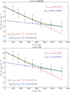 |
Fig. 1 Example of the H2 excitation diagram analysis with pdrtpy of source mmA1 (top) and source B (bottom). The observed data are shown in black and the two-component fit is shown by red and blue dots, which correspond to the warm and hot component, respectively, and the total fit is indicated by a green line. |
Line-integrated intensities of H2 (extinction-corrected, adopting values of AK = 7, 5, and 3 mag) derived from a Gaussian fit to the observed line profiles (Sect. 3.3).
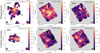 |
Fig. 2 Temperature and H2 column density of the gas components in IRAS 23385 derived using CH3CN and H2 as a diagnostic tool (Sects. 3.3 and 3.4). In the top and bottom panels, the rotation temperature and H2 column density maps, respectively, of the cold (left), warm (center), and hot (right) components are shown in color. The angular resolution of the line data is indicated by a purple ellipse in the bottom right corner. The JWST/MIRI 5.2 µm continuum is presented by blue contours with contour levels at 5, 10, 15, 20, and 25 × σcont,5 µm and the angular resolution is highlighted by a black ellipse in the bottom left corner. The NOEMA 3 mm continuum (top and bottom left panels) is highlighted by gray contours with levels at 5, 10, 20, 40, and 80 × σcont,3 mm and the synthesized beam is highlighted by a gray ellipse in the bottom left corner. All continuum sources are labeled in green in the bottom left panel and the millimeter continuum sources are marked by green squares. Several shock positions are indicated by green crosses (Sect. 3.2). |
Fit results from the H2 excitation diagram analysis with pdrtpy (Sect. 3.3) with a warm and hot component, adopting values of AK = 7, 5, and 3 mag.
References
- Gieser, C., Beuther, H., van Dishoeck, E. F., et al. 2023, A&A, 679, A108 [NASA ADS] [CrossRef] [EDP Sciences] [Google Scholar]
- Nisini, B., Giannini, T., Neufeld, D. A., et al. 2010, ApJ, 724, 69 [NASA ADS] [CrossRef] [Google Scholar]
© The Authors 2024
 Open Access article, published by EDP Sciences, under the terms of the Creative Commons Attribution License (https://creativecommons.org/licenses/by/4.0), which permits unrestricted use, distribution, and reproduction in any medium, provided the original work is properly cited.
This article is published in open access under the Subscribe to Open model.
Open Access funding provided by Max Planck Society.
All Tables
Line-integrated intensities of H2 (extinction-corrected, adopting values of AK = 7, 5, and 3 mag) derived from a Gaussian fit to the observed line profiles (Sect. 3.3).
Fit results from the H2 excitation diagram analysis with pdrtpy (Sect. 3.3) with a warm and hot component, adopting values of AK = 7, 5, and 3 mag.
All Figures
|
Fig. 1 Example of the H2 excitation diagram analysis with pdrtpy of source mmA1 (top) and source B (bottom). The observed data are shown in black and the two-component fit is shown by red and blue dots, which correspond to the warm and hot component, respectively, and the total fit is indicated by a green line. |
| In the text | |
|
Fig. 2 Temperature and H2 column density of the gas components in IRAS 23385 derived using CH3CN and H2 as a diagnostic tool (Sects. 3.3 and 3.4). In the top and bottom panels, the rotation temperature and H2 column density maps, respectively, of the cold (left), warm (center), and hot (right) components are shown in color. The angular resolution of the line data is indicated by a purple ellipse in the bottom right corner. The JWST/MIRI 5.2 µm continuum is presented by blue contours with contour levels at 5, 10, 15, 20, and 25 × σcont,5 µm and the angular resolution is highlighted by a black ellipse in the bottom left corner. The NOEMA 3 mm continuum (top and bottom left panels) is highlighted by gray contours with levels at 5, 10, 20, 40, and 80 × σcont,3 mm and the synthesized beam is highlighted by a gray ellipse in the bottom left corner. All continuum sources are labeled in green in the bottom left panel and the millimeter continuum sources are marked by green squares. Several shock positions are indicated by green crosses (Sect. 3.2). |
| In the text | |
Current usage metrics show cumulative count of Article Views (full-text article views including HTML views, PDF and ePub downloads, according to the available data) and Abstracts Views on Vision4Press platform.
Data correspond to usage on the plateform after 2015. The current usage metrics is available 48-96 hours after online publication and is updated daily on week days.
Initial download of the metrics may take a while.