| Issue |
A&A
Volume 673, May 2023
|
|
|---|---|---|
| Article Number | A121 | |
| Number of page(s) | 12 | |
| Section | Interstellar and circumstellar matter | |
| DOI | https://doi.org/10.1051/0004-6361/202346167 | |
| Published online | 18 May 2023 | |
JWST Observations of Young protoStars (JOYS)
Outflows and accretion in the high-mass star-forming region IRAS 23385+6053★
1
Max Planck Institute for Astronomy,
Königstuhl 17,
69117
Heidelberg,
Germany
e-mail: This email address is being protected from spambots. You need JavaScript enabled to view it.
2
Leiden Observatory, Leiden University,
PO Box 9513,
NL 2300
RA Leiden,
The Netherlands
3
European Southern Observatory,
Karl-Schwarzschild-Strasse 2,
85748
Garching bei München,
Germany
4
Max Planck Institute for Extraterrestrial Physics,
Gießenbachstrasse 1,
85748
Garching,
Germany
5
School of Cosmic Physics, Dublin Institute for Advanced Studies,
31 Fitzwilliam Place,
Dublin 2,
Ireland
6
UK Astronomy Technology Centre, Royal Observatory Edinburgh,
Blackford Hill,
Edinburgh
EH9 3HJ,
UK
7
INAF-Osservatorio Astronomico di Capodimonte,
Salita Moiariello 16,
80131
Napoli,
Italy
8
Laboratory for Astrophysics, Leiden Observatory, Leiden University,
PO Box 9513,
NL 2300
RA Leiden,
The Netherlands
9
Department of Space, Earth and Environment, Chalmers University of Technology, Onsala Space Observatory,
439 92
Onsala,
Sweden
10
Instituut voor Sterrenkunde, KU Leuven,
Celestijnenlaan 200D, Bus-2410,
3000
Leuven,
Belgium
11
Centro de Astrobiologia (CAB, CSIC-INTA),
Carretera de Ajalvir,
28850
Torrejon de Ardoz, Madrid,
Spain
12
DTU Space, Technical University of Denmark.
Building 328, Elektrovej,
2800 Kgs.
Lyngby,
Denmark
13
Department of Astrophysics, University of Vienna,
Türkenschanzstr. 17,
1180
Vienna,
Austria
14
ETH Zürich, Institute for Particle Physics and Astrophysics,
Wolfgang-Pauli-Str. 27,
8093
Zürich,
Switzerland
15
Université Paris-Saclay, Université de Paris, CEA, CNRS, AIM,
91191
Gif-sur-Yvette,
France
16
Department of Astronomy, Oskar Klein Centre, Stockholm University,
106 91
Stockholm,
Sweden
Received:
17
February
2023
Accepted:
22
March
2023
Abstract
Context. Understanding the earliest stages of star formation, and setting it in the context of the general cycle of matter in the interstellar medium, is a central aspect of research with the James Webb Space Telescope (JWST).
Aims. The JWST program JOYS (JWST Observations of Young protoStars) aims to characterize the physical and chemical properties of young high- and low-mass star-forming regions, in particular the unique mid-infrared diagnostics of the warmer gas and solid-state components. We present early results from the high-mass star formation region IRAS 23385+6053.
Methods. The JOYS program uses the Mid-Infrared Instrument (MIRI) Medium Resolution Spectrometer (MRS) with its integral field unit (IFU) to investigate a sample of high- and low-mass star-forming protostellar systems.
Results. The full 5–28 µm MIRI MRS spectrum of IRAS 23385+6053 shows a plethora of interesting features. While the general spectrum is typical for an embedded protostar, we see many atomic and molecular gas lines boosted by the higher spectral resolution and sensitivity compared to previous space missions. Furthermore, ice and dust absorption features are also present. Here, we focus on the continuum emission, outflow tracers such as the H2(0–0)S(7), [FeII](4F9/2−6D9/2), and [NeII](2P1/2−2P3/2) lines, and the potential accretion tracer Humphreys α H I(7−6). The short-wavelength MIRI data resolve two continuum sources, A and B; mid-infrared source A is associated with the main millimeter continuum peak. The combination of mid-infrared and millimeter data reveals a young cluster in the making. Combining the mid-infrared outflow tracers H2, [FeII], and [NeII] with millimeter SiO data reveals a complex interplay of at least three molecular outflows driven by protostars in the forming cluster. Furthermore, the Humphreys α line is detected at a 3–4σ level toward the mid-infrared sources A and B. One can roughly estimate both accretion luminosities and corresponding accretion rates to be between ~2.6 × 10⁻⁶ and ~0.9 × 10⁻⁴ M⊙ yr−1. This is discussed in the context of the observed outflow rates.
Conclusions. The analysis of the MIRI MRS observations for this young high-mass star-forming region reveals connected outflow and accretion signatures, as well as the enormous potential of JWST to boost our understanding of the physical and chemical processes at play during star formation.
Key words: stars: formation / ISM: clouds / ISM: individual objects: IRAS23385+6053 / stars: jets / stars: massive
Data (FITS files) are available at the CDS via anonymous ftp to cdsarc.cds.unistra.fr (130.79.128.5) or via https://cdsarc.cds.unistra.fr/viz-bin/cat/J/A+A/673/A121
© The Authors 2023
 Open Access article, published by EDP Sciences, under the terms of the Creative Commons Attribution License (https://creativecommons.org/licenses/by/4.0), which permits unrestricted use, distribution, and reproduction in any medium, provided the original work is properly cited.
This article is published in open access under the Subscribe to Open model.
Open Access funding provided by Max Planck Society.
1 Introduction
The earliest phases of protostellar evolution proceed deeply embedded in their natal cloud cores. Many important physical and chemical processes occur there, including the infall of the envelope, the formation of disks and outflows, the main accretion phase and growth of the final star, and the chemical enrichment of the disk directly impacting planet formation. Because of the very high extinction, AV, of several hundred or even thousands of magnitudes, these deeply embedded phases have to be studied at (mid-)infrared and (sub)millimeter wavelengths. While (sub)millimeter interferometers have allowed detailed imaging of the cold material in such star-forming cores (for a review, see Motte et al. 2018), mid-infrared continuum and line imaging of the warmer material at subarcsecond spatial resolution has been barely feasible so far. Only a few space-based studies at lower angular resolution with the Infrared Space Observatory (ISO) and Spitzer are reported (e.g., Whittet et al. 1996; van Dishoeck et al. 1998;Gibb et al. 2000;Molinari et al. 2008;An et al. 2011). The most comprehensive ISO legacy study on high-mass protostars is presented in Gibb et al. (2004).
The situation has now changed dramatically with the advent of the James Webb Space Telescope (JWST), launched on December 25, 2021, just a little more than a year ago at the time of writing. Scientific data delivery began only in July 2022, and we present the first results from the European Mid-Infrared Instrument (MIRI) Guaranteed Time Program JWST Observations of Young protoStars (JOYS; PI: E. F. van Dishoeck, pid 1290).
The JOYS program observes a total of about two dozen low-to high-mass star-forming regions with the MIRI Medium Resolution Spectrometer (MRS) and its integral field unit (IFU) to address a broad range of scientific topics. Evolutionary stages from very young embedded protostars within infrared-dark clouds to Class 0/I protostars as well as high-mass protostel-lar objects and hot molecular cores are being covered by the JOYS project. The spatial resolution of the MIRI instrument of ~ 0.19″, ~ 0.58″, and ~ 0.96″ at 5, 15, and 25 µm, respectively, corresponds, at typical distances of the low-mass cores of ~ 150 pc, to linear resolution elements of ~29, ~87, and ~ 144 au. For high-mass regions at more typical distances of ~3 kpc, the linear resolution corresponds roughly to 570, 1740, and 2880 au.
We use a set of key diagnostics in the mid-infrared band between 5 and 28 µm, including the continuum spectral energy distribution, a range of atomic and molecular gas lines, and several solid-state bands. More details about the JOYS project will be presented in a forthcoming publication by van Dishoeck et al., (in prep.).
Here, we focus on analyzing and interpreting JWST data of the first source fully observed within the JOYS program, the high-mass protostellar object IRAS 23385+6053. This high-mass star-forming region was originally identified by IRAS (Infrared Astronomical Satellite) color selection and association with H2O maser emission (Casoli et al. 1986;Cesaroni et al. 1988;Wouterloot & Brand 1989;Palla et al. 1991). Early interferometric investigations revealed that the region is embedded in a comparatively dark cloud core surrounded by larger-scale mid-infrared emission (Molinari et al. 1998). Figure 1 presents an overview of the region at 12 µm (left panel), from the Wide-field Infrared Survey Explorer (WISE) mission at 6.5″ resolution (Wright et al. 2010), and 1.3 mm emission (right panel;Beuther et al. 2018, Cesaroni et al. 2019), showing the large-scale extended mid-infrared emission that weakens at the positions of the central bright millimeter emission. The outline of the four-field MIRI-IFU coverage is shown there as well. The υlsr of the region is −50.2 km s−1. At a kinematic distance of 4.9 kpc, the total luminosity measured with the IRAS mission accounts for 1.6 × 10⁴ L⊙ (Molinari et al. 1998). However, higher-spatial-resolution Spitzer/MIPSGAL observations revealed that only ~3 × 10³ L⊙ is associated with the central core, consistent with a high-mass protostar in the main accretion phase (Molinari et al. 2008). Infrared imaging by Faustini et al. (2009) revealed an infrared cluster in the surroundings of the region. A weak K-band source is detected in their data toward the very center (Fig. 2). An H2 emission-line study at 2.12 µm revealed shocked H2 emission in the immediate surroundings of the central millimeter-core (Wolf-Chase et al. 2012). CH3OH maser emission at 44 and 95 GHz confirms shock emission in IRAS 23385+6053 (Kurtz et al. 2004;Wolf-Chase et al. 2012). The most recent high-spatial-resolution millimeter observations (~O.4″) were conducted within the IRAM Northern Extended Millimeter Array (NOEMA) large program CORE, which studied the physical and chemical properties of 20 high-mass star-forming regions (Beuther et al. 2018;Gieser et al. 2021). A detailed case study of IRAS 23385+6053 from the CORE project is presented in Cesaroni et al. (2019). Based on the line and continuum emission, Cesaroni et al. (2019) identified six cores, a new outflow candidate in the northwest-southeast direction (Fig. 1, middle panel), and a tentative detection of a disk around a ~9 M⊙ protostar within the most massive millimeter core, mmA1 (Fig. 1, right panel).
This first paper in the JOYS series presents an overview of the MIRI spectrum and then focuses on the continuum emission and a few selected molecular and atomic lines (H2(0– 0)S(7), [FeII](4F9/2−6D9/2), [NeII](2P1/2−2P3/2) and Humphreys α H I(7−6)). The data allow us to outline the general source structure, and we investigate the outflow properties and potential accretion signatures. Forthcoming articles in this series will discuss the overall extended emission of the diverse set of detected atomic and H2 lines and set them in relation to the molecular gas properties derived at millimeter wavelengths (Gieser et al., in prep.), the molecular emission around the central disk candidate (Francis et al., in prep.), and the ice properties in the region (Rocha et al., in prep.).
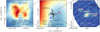 |
Fig. 1 Overview of the region around IRAS 23385+6053. The left panel shows a large-scale overview, and the middle and right panels present zoomed-in views. The color scale in the left and middle panels shows the 12 µm emission from WISE at an angular resolution of 6.5″ (Wright et al. 2010). The little squares outline the field of view of the MIRI IFU mosaic in channel 1 (each square is 3.7″ × 3.7″). The color scale in the right panel shows the new MIRI 5.2 µm continuum emission (see also Fig. 4). The contours in the middle and right panels present the 1.3 mm continuum emission (Beuther et al. 2018;Cesaroni et al. 2019). The contours start at the 5σ level of 0.55 mJy beam−1 and continue in 25σ steps. The black lines and red and blue lines in the middle panel show the directions of outflows identified in Molinari et al. (1998) and Cesaroni et al. (2019), respectively. The right panel marks the mid-infrared sources A and Β as well as the millimeter sources labeled “mm” with the corresponding source letters from Cesaroni et al. (2019). Mid-infrared source A and millimeter source mm A2 are spatially colocated. A linear scale-bar is shown in all panels. |
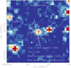 |
Fig. 2 Infrared K-band data shown in color (taken with the Palomar 60-inch telescope and the NICMOS-3 array;Faustini et al. 2009). The contours outline the 1.3 mm emission (Beuther et al. 2018;Cesaroni et al. 2019). Contour levels start at 5σ (0.55 mJy beam−1) and continue in 25σ steps. The solid and dashed white lines show the directions of outflows identified in Molinari et al. (1998) and Cesaroni et al. (2019), respectively. |
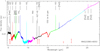 |
Fig. 3 Full MIRI spectrum extracted toward the combined sources A and B (central position: RA (J2000.0) 23:40:54.49, Dec 61:10:27.4) within a diameter of 2.4″. The color coding separates the different sub-bands from channel 1 short to channel 4 long. Prominent strong atomic and molecular lines are labeled (see Table 1). The four main lines discussed in this paper are highlighted by the red arrows at the bottom. The data are not background-subtracted. The error bars at 19 and 21 µm show the approximate 1σ rms below and above 20 µm of ~0.5 and ~2 mJy (note the log-scale), respectively (Sect. 2). |
2 Observations
IRAS 23385+6053 was observed within the European MIRI Guaranteed Time Observations (GTO) program JOYS (proposal ID 1290) for 2.12 h on August 22, 2022. The entire MIRI bandpass from ~4.9 to ~28.0 µm was covered in a 4-field mosaic (Fig. 1) around the central position of right ascension (RA; J2000.0) 23:40:54.497 and declination (Dec; J2000.0) +61:10:27.83. The total exposure time in each the three MIRI spectral filters was 200 sec, and parallel off-source imaging was conducted in the F1500W filter. A complementary background field was observed for overall background subtraction that is needed, for example an analysis of the broadband ice features. While the full-wavelength spectrum in Fig. 3 shows the non-background-subtracted data, all individual narrow gas spectral line data presented in this paper were continuum-subtracted by fitting a polynomial baseline to narrow wavelength ranges around these lines.
We reduced the data using a development version of the JWST calibration pipeline (Bushouse et al. 2022) with v. 11.16.16 and Calibration Reference Data System (CRDS) context “jwst_1017.pmap”, respectively. We used this development version as it includes cosmic ray shower flagging in the jump step of the DetectorlPipeline.
The pipeline includes fringe correction via Spec2Pipeline using a fringe flat field derived from spatially extended sources (Mueller et al., in prep.). We further reduced the fringing by applying the residual_fringe step (Kavanagh et al., in prep.), which is included in the JWST calibration pipeline package but not switched on by default.
As discussed in Pontoppidan et al. (2022), the accuracy of spacecraft pointing information for MRS exposures can be affected by guide star catalog errors and roll uncertainty. We corrected our MRS exposures following the same procedure as in that paper, that is, using identified Gaia Data Release 31 sources in the MIRI simultaneous imaging field, which led to a pointing adjustment of 1.6077″ in RA and 0.3485″ in Dec. This correction is still subject to uncertainties in the relative astrometry between the imager and the MRS, which is expected to be accurate to ≤0.1″ (Patapis et al., in prep.).
Finally, we created spectral cubes for each of the 12 MRS sub-bands (four MIRI channels with each containing a “short”, “medium”, and “long” grating setting) using the level 2 data products with corrected astrometry from which spectra were extracted. We applied the post-pipeline residual fringe correction tool to all spectra to account for high frequency fringe residuals, thought to originate in the MRS dichroics, which are not effectively removed by the residual_fringe step in the pipeline (Kavanagh et al., in prep.). The 1σ rms of the spectrum presented in Fig. 3 is typically around 0.5 mJy below 20 µm and rises to a few millijanskys at longer wavelengths.
Complementary 1.3 mm continuum data are used from the CORE project (Beuther et al. 2018;Cesaroni et al. 2019). The angular resolution and sensitivity of these data are 0.48″ × 0.43″ and 0.11 mJy beam−1, respectively. Furthermore, SiO(2−1) observations are taken from the CORE follow-up project CORE+ (PI: Caroline Gieser). This project aims to study the shock and deuterium chemistry in the CORE sample. IRAS 23385+6053 is part of the CORE+ pilot study (Gieser et al., in prep.). The corresponding angular resolution and sensitivity of the SiO(2−1) data are 1.4″ × 1.2″ and ~0.12 K per 0.8 km s−1, respectively.
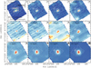 |
Fig. 4 Continuum images of IRAS 23385+6053. The color scale presents the continuum emission extracted from the MIRI-IFU data cube in a line-free part of each spectral setting centered on the wavelength labeled in each panel. The contours outline the 1.3 mm emission (Beuther et al. 2018;Cesaroni et al. 2019) starting at the 5σ level of 0.55 mJy beam−1 and continuing in 25σ steps. In the top right of each panel, the corresponding spatial resolution is shown (gray: mid-infrared, line: 1.3 mm). In the top-left panel, the two main mid-infrared sources, A and B, are labeled, and the main millimeter peak from Cesaroni et al. (2019), mmA1, is marked with with a green star. A linear scale-bar is shown as well. Note that mid-infrared sources A and B are well separated up to 8 µm, but not at longer wavelengths. |
3 Results
3.1 General spectral features
Figure 3 presents the spectrum extracted toward the combined emission from the two mid-infrared sources A and B (Sect. 3.2 and Fig. 4). We present the combined spectrum from sources A and B because at wavelengths longward of ~ 13 µm, they cannot be spatially separated anymore (Fig. 4). The color-coding corresponds to the four MIRI channels with the corresponding three grating settings each, hence 12 individual sub-bands. It is evident that JWST can now take high-quality mid-infrared spectra of sources as weak as 10 mJy in short integration times, more than a factor of 1000 fainter than previous data. Several features can directly be identified (see Table 1). Between ~5 and ~11.5 µm, the spectrum is dominated by well-known structures that stem from several ice and solid-state features (e.g., Gibb et al. 2004;Yang et al. 2022;McClure et al. 2023). In particular, the silicate band around 10 µm shows strong absorption, almost reaching full saturation. Going to longer wavelengths, the general emission rises as expected from warm dust emission. On top of the continuum emission, ice and solid-state features, as well as many strong emission lines, can be identified, in particular from H2 and atomic lines from [FeII], [ArII], [NiII], [NeII], and [SI] (all labeled in Fig. 3). In addition to these strong lines, also a few weaker molecular lines can be identified, in particular those of CO2, C2H2, CH4, and HCN (Francis et al., in prep.). While the H2 and atomic line emission is extended, the molecular emission mainly stems from the environment of the continuum sources. Selected H2, [FeII] and [NeII] line images are presented in Sect. 3.3, whereas the remaining gas and ice analysis will be discussed in accompanying papers (Sect. 1).
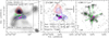 |
Fig. 5 Outflow images in NOEMA SiO(2−1) (integrated emission, left panel), JWST [FeII](4F9/2−6D9/2) at 5.34 µm (middle panel), and JWST H2(0–0)S(7) at 5.511 µm (right panel). The red and blue contours show the redshifted and blueshifted NOEMA SiO(2−1) emission in the labeled velocity regimes (υlsr = −50.2 km s−1). Contour levels are from 30 to 90% (steps of 10%) of the respective integrated peak emission. The magenta contours show the 5.2 µm continuum emission (steps 20–90% by 15%). The green contours in the left panel outline the 1.3 mm continuum starting at the 20σ levels (1σ = 1.13 mJy beam−1). A linear scale-bar is presented in the middle panel, and the green lines in the right panel outline and label potential outflows. The two mid-infrared sources are labeled in the right panel as well. The dashed line in the left panel marks a potentially precessing outflow corresponding to outflow (I). A green star in all panels marks the main millimeter peak position labeled mmA1 in Cesaroni et al. (2019). North and west are labeled in the right panel. The resolution elements are shown at the bottom right of each panel. Left: SiO(2−1) in gray and the 1.3 mm continuum as a line. Middle: [FeII]. Right: H2. |
Main spectral features.
3.2 Continuum emission
Figure 4 presents the mid-infrared continuum emission extracted for each of the twelve MIRI sub-bands averaged over wavelength ranges without significant line emission. The central wavelengths of each image are marked in all panels. We show the mid-infrared emission in comparison to the millimeter continuum emission from the CORE project (Beuther et al. 2018, Cesaroni et al. 2019; see also Fig. 1 for more detailed source labels). At the short wavelengths, one clearly identifies two mid-infrared sources associated with the main millimeter continuum core. That is also the area where the K-band emission is detected (Faustini et al. 2009, Fig. 2). The northwestern mid-infrared source A is closer to the main millimeter peak position (mmA1 in Cesaroni et al. 2019) whereas the southeastern source, B, is offset from mid-infrared source A by ~0.67″. At the given distance of 4.9 kpc, the angular offset between the two mid-infrared sources A and B corresponds to a projected linear separation of ~3280 au.
While the offset between the mid-infrared sources A and B is well determined, the absolute positional offsets between the millimeter and mid-infrared data are less well constrained. Positions from millimeter interferometer observations like the NOEMA CORE data (Beuther et al. 2018) are largely constrained by the phase error, and should be better than 0.1″ for the presented millimeter data. The corresponding 3 mm continuum data do also agree very well with the 1.3 mm data presented here (Gieser et al., in prep.). In contrast to that, the mid-infrared positional accuracy depends on the absolute JWST pointing, and the accuracy with which the data can be improved by using known Gaia positions during the data reduction. As outlined in Sect. 2, after correlating the parallel imaging data with Gaia observations, the data were shifted in RA and Dec. by ~1.6077″/0.3485″. In addition to the alignment with Gaia, this correction needs additional knowledge of the alignment of the MIRI imager with the MIRI-IFU. This alignment should be very good and accurate to 0.1″ (Sect. 2). This implies that mid-infrared source A should indeed be very close to the elongation of the main millimeter peak (the millimeter elongation is labeled peak mmA2 in Cesaroni et al. 2019) whereas the offset of mid-infrared source B to the southeast should be real as well.
Going to longer wavelengths, in the spectral range of the silicate feature between roughly 9 and 11 µm, source B almost disappears. This indicates that the silicate absorption feature toward source B is even deeper and entirely absorbs the continuum emission, whereas for source A some continuum emission still remains. A detailed analysis of all solid-state features will be presented in Rocha et al. (in prep.). Moving to even longer wavelengths beyond the silicate feature, source B reappears. From ~ 16 µm onward, the further decreasing spatial resolution does not allow us to separate the two mid-infrared sources anymore, and they merge into a single source at the long-wavelength end of the MIRI bandpass.
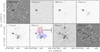 |
Fig. 6 Channel map of the H2(0–0) S(7) line at 5.511 µm. The velocity of each channel is marked in units of km s−1 in the top-left corner of the panels. The red and blue contours in the 33 km s−1 channel correspond to the same redshifted and blueshifted SiO(2−1) emission as presented in Fig. 5. A linear scale-bar is shown in that panel as well. The υlsr is −50.2 km s−1. |
3.3 H2, [Fell], and [Nell] line emission
The MIRI spectral line data now allow us to get a better understanding of the underlying outflow structures in IRAS 23385+6053. While Molinari et al. (1998) reported one outflow roughly in the north-south direction, Cesaroni et al. (2019) recently suggested that a second outflow in the northwest-southeast direction should also exist (Fig. 1, right panel). The shocked H2 emission as well as CH3OH maser emission at 44 and 95 GHz additionally confirm the existence of shocked gas (Kurtz et al. 2004;Wolf-Chase et al. 2012). Here, we focus on the high-spatial-resolution H2(0–0) S(7) line at 5.511 µm and the [FeII](4F9/2−6D9/2) line at 5.34 µm. Furthermore, we compare the results with SiO(2−1) data at 3.6 mm wavelengths obtained with NOEMA as part of the CORE+ project (Gieser et al., in prep.). Figure 5 presents a compilation of the three data sets. For the SiO(2−1) data, we show the integrated emission (±15 km s−1 around the υlsr = −50.2 km s−1) as well as separated blueshifted and redshifted high-velocity gas emission, whereas for [FeII] and H2 we present the integrated emission.
Starting with the millimeter SiO emission, these data are compatible with at least two outflows. The integrated SiO(2−1) emission (grayscale in Fig. 5, left) is consistent with the northwest-southeast outflow ((I) in Fig. 5, right panel) proposed by Cesaroni et al. (2019). The SiO emission also shows a more extended integral-shaped structure in the northwest-southeast direction (dashed line in Fig. 5, left; see the discussion in Sect. 4.2). In comparison, the redshifted and blueshifted SiO emission rather points at an outflow more aligned with the north-south direction ((IIa) & (IIb) in Fig. 5, right panel) as suggested by Molinari et al. (1998). However, especially the blueshifted SiO emission shows extensions toward the east and west that may also be associated with other outflow structures.
The [FeII] emission (Fig. 5, middle) exhibits a very different structure. It is dominated by a collimated jet-like outflow in the northeast-southwest direction ((III) in Fig. 5, right panel). But it also shows some extension toward the west, spatially associated with the blueshifted SiO emission.
Last but not least, the H2 data (Fig. 5, right) show emission structures associated with all the above mentioned outflows. There is strong emission associated with the northeast-southwest jet (III) traced also in [FeII], but it shows additional emission toward the northwest, similar to the integrated SiO emission (I). Furthermore, the H2 data also exhibit strong emission toward the north (labeled (IIa) and (IIb) in Fig. 5, right panel), and slightly weaker in the south, that corresponds to the redshifted and blueshifted SiO emission.
In addition to the integrated emission, with a spectral resolving power of ~3500 in channel 1A (Labiano et al. 20212), we can resolve velocity elements down to ~86 km s−1 (corrected for radial and heliocentric velocities). With an approximate Nyquist-sampling the channel separation is ~44 km s−1. Figure 6 presents a channel map for the H2 line at 5.511 µm. Interestingly, the gas velocities are indeed so high that we can velocity-resolve the different components. With the ilsr of IRAS 23385+6053 of −50.2 km s−1 (Beuther et al. 2018), we are covering a velocity range of roughly ±140 km s−1. For comparison, we also present the channel map of the [FeII] line at 5.34 µm in Fig. 7. Again, we can resolve blueshifted and redshifted gas, albeit with a slightly smaller velocity spread of around ±100 km s−1.
Investigating the velocity structures in a bit more detail, we find that the H2 emission features toward the north are all redshifted. This is consistent with the redshifted SiO emission – although SiO is at lower velocities – that is also found in the north (Fig. 5). In contrast to that, the strong H2 emission in the northeast is seen in all velocity channels, hence redshifted and blueshifted. If we assign that feature to the northeast-southwest jet (III) that is also seen nicely in the [FeII] emission (Figs. 5 and 7), this implies that this jet should be aligned close to the plane of the sky. The outflow (I) in the northwest-southeast direction can also be identified in the H2 channel map (Fig. 6), notably at redshifted velocities; it is barely visible in the blueshifted gas. This velocity structure is not well recovered in the SiO emission (Fig. 5)
Another potential jet-tracer is the [NeII](2P1/2−2P3/2) line at 12.814 µm (e.g., Hollenbach & McKee 1989;Lefloch et al. 2003). Figure 8 presents a comparison of the [NeII] and the [FeII] emission, and one finds two spatially very different distributions. While the [FeII] emission mainly traces the northeast-southwest oriented collimated jet-like structure, the [NeII] emission is rather double-peaked with one peak centered on mid-infrared source A, whereas the second [NeII] emission peak is offset by ~0.9″ to the west. Comparing the [NeII] emission directly to the [FeII], one finds weak [FeII] emission associated also with the secondary [NeII] peak (left panel of Fig. 8). This [FeII] emission arises mainly at relatively high projected red-shifted velocities (see channels at −22 and +22 km s−1 in Fig. 7). We note that no clear velocity structure can be spectrally resolved in the [NeII] data. The [NeII] emission can stem from extreme-UV- and/or X-ray-irradiated surface layers of accretion disks as well as from jets and outflows (e.g., Hollenbach & McKee 1989;Lefloch et al. 2003;Glassgold et al. 2007;Pascucci & Sterzik 2009;Guedel et al. 2010). The J-shock models by Hollenbach & McKee (1989) predict that the [NeII] emission should strongly increase for gas velocities greater than ~80 km s−1. In addition to this, high densities are also increasing the [NeII] intensities in these shock models (Fig. 7 in Hollenbach & McKee 1989). The spatial correspondence of the high-velocity redshifted [FeII] and [NeII] emission close to the center of the region, where gas densities are also highest, is consistent with these J-shock models. In addition to this, these regions close to the central protostars, traced by the mid-infrared continuum emission, should also be exposed most to UV radiation. Hence, a combination of fast shocks and UV radiation may favor the [NeII] emission in that region. The non-detection of compact [NeII] emission in the rest of the IRAS 23385+6053 region, where partly also high gas velocities and/or dense gas are observed (e.g., Figs. 1 and 6), confirms that not only high velocities and dense gas are important, but that the missing UV radiation further away from the main protostars is likely to play an important role as well.
In summary, the combination of these data sets reveals at least three outflows, one in the northwest-southeast direction (I), another in the northeast-southwest direction (III) and at least one more in the north-south direction (IIa and IIb). The fact that the H2 emission shows two emission peaks in the north can be explained by either an expanding outflow cavity of one outflow or alternatively by two more jet-like structures. Differentiating between these two scenarios is not possible with the given data. The three, or potentially even four outflows are marked with white lines in Fig. 5 (right panel).
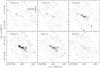 |
Fig. 7 Channel map of the Fe[II](4F9/2−6D9/2) line at 5.34 µm. The velocity of each channel is marked in units of km s−1 in the top-left corner of the panels. A linear scale-bar is shown in the top-left panel. The υlsr is −50.2 km s−1. |
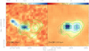 |
Fig. 8 Integrated [Fell](4F9/2−6D9/2) (left) and [Nell](2P1/2−2P3/2) (right) emission. The black contours show the 5.2 µm continuum emission (steps of 10% from 20% to 90%). The green contours again outline the [NeII] emission in 10σ steps (1σ ~ 0.09 MJy sr−1 µm). |
3.4 Humphreys α line emission as a possible accretion tracer
One crucial missing parameter in high-mass star formation is the actual accretion rate onto the protostars. Here, we differentiate the accretion rate onto the protostar from otherwise more typically reported gas infall rates within the protostellar envelopes and cores (e.g., Myers et al. 1996;Mardones et al. 1997;Beuther et al. 2013;Wyrowski et al. 2016; van Dishoeck et al. 2021). While for low-mass T Tauri stars the accretion rate can be measured with optical or near-infrared lines (e.g., Connelley & Greene 2010;Salyk et al. 2013;Hartmann et al. 2016;Alcalá et al. 2017), for the deeply embedded phases in low- and highmass star formation, one has to resort to longer wavelengths. Here, we focus on the Humphreys α line H I(7−6) at 12.37 µm. Rigliaco et al. (2015) explored this H I(7−6) line at 12.37 µm in Spitzer data of classical T Tauri stars, and they found a tentative correlation between the integrated H I(7−6) luminosity and the accretion luminosity. We now explore this relation also for IRAS 23385+6053. Figure 9 presents the spectrum of the H I(7−6) line extracted from the position in between mid-infrared sources A and B, and averaged over an aperture with radius of 2″. While the red line shows a single Gaussian fit, the blue line presents a two-component Gaussian fit. It should be noted that at this stage we consider this only a tentative detection, even though the peak flux density of the single-Gaussian fit with a peak flux density of 0.61 mJy reaches a signal-to-noise ratio S /N of 3 (in the channel with highest flux densities even S /N ~ 4.1). The peak flux densities of the two-component fit (peak flux densities of 0.78 and 0.65 mJy, respectively) have nominal S/N ratios of 3.8 and 3.2, respectively.
With a nominal central wavelength for the H I(7−6) line of 12.3719 µm, the two components are shifted by −70 and +293 km s−1, respectively. The full-width-half-maximum line-widths of the two components are ~73 and ~436 km s−1, respectively. While the two-component nature of the spectrum may be attributed to gas associated with the innermost red-shifted and blueshifted rotating gas, the line-width of several hundred km s−1 is consistent with gas at almost free-fall onto the central protostar. The free-fall velocity of gas around a 9 M⊙ protostar (Cesaroni et al. 2019) with a radius of 5 R⊙ would be ~829 km s−1, but is likely smaller if the protostar were significantly bloated (e.g., Hosokawa & Omukai 2009).
Assuming this to be a real detection, we can derive the integrated flux values of the one- and two-component fits. Since the integrated values of the different fits are similar, the following analysis is done for the two-component fit. However, with the single-component fit one gets comparable results. The integrated line luminosity of the two-component Gaussian fit is ~ 2.3 × 10⁻⁴ L⊙. This value lies at the high-luminosity end of the relation fitted by Rigliaco et al. (2015) to a sample of low-mass protostars. This then could be interpreted as an indicator that this relation may also extend to the high-mass regime.
Following Eq. (1) in Rigliaco et al. (2015), one can convert the line luminosity to an accretion luminosity of 142 L⊙. Assuming now that all that luminosity is from infalling gas that converts its energy to radiation, one can infer an estimate of the accretion rate, for example Eq. (11.5) in Stahler & Palla (2005). Taking these numbers at face-value, for an 9 M⊙ protostar (Cesaroni et al. 2019) with a radius of 5 R⊙ we can estimate an accretion rate of ~2.6 × 10⁻⁶ M⊙ yr−1.
The above fitted integrated line luminosity is a lower limit since extinction may weaken the real line emission. We now estimate an extinction correction using the extinction curve derived by McClure (2009). Based on the 9.7 µm silicate absorption feature, Rocha et al., (in prep.) estimate an extinction AV ~ 30–40 mag. Using AV ~ 30 mag, and following McClure (2009), that extinction can be converted to a K-band AK and then 12.37 µm extinction values of 3.8 and 1.86 mag, respectively. Such a 12.37 µm extinction would boost the integrated H I(7−6) line luminosity by a factor of ~5.56. Using the same approach as above, one can estimate now an extinction-corrected accretion luminosity of ~5070 L⊙ and an accretion rate of ~0.9 × 10⁻⁴ M⊙ yr−1. The latter is roughly a factor of 36 higher than the estimate without the extinction correction.
One caveat is that the extinction-corrected accretion luminosity of ~ 5070 L⊙ is on the same order as the luminosity estimated for the source of ~3000 L⊙ (Molinari et al. 2008). Because of that, higher accretion luminosities would be unreasonable, and correspondingly, we do not consider higher extinction values. This accretion luminosity would imply that most of the bolometric luminosity originates from accretion; thus, the source could be in its main accretion phase. If the approach outlined by Rigliaco et al. (2015) and followed here is also applicable for young high-mass protostars, the extinction-corrected accretion rate estimate has to be an upper limit to the real accretion rate onto the protostar. The accretion rates will be discussed in depth in Sect. 4.3.
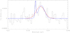 |
Fig. 9 H I(7−6) spectrum at 12.37 µm centered right in the middle between sources A and B (Fig. 4) and averaged over an aperture with radius 2″. The red line presents a single Gaussian fit to the spectrum, whereas the blue line shows a two-component Gaussian fit to the spectrum. |
4 Discussion
4.1 Embedded protostars
This leads us to questions regarding the nature of the two mid-infrared sources, A and B, more specifically as to whether they are individual protostars or potentially part of an extended disklike structure perpendicular to the northeast-southwest outflow best depicted in the [FeII] data (Fig. 5).
The spatial separation between sources A and B of 0.67″ corresponds at the measured distance of 4.9 kpc to a linear separation of ~3300 au. This seems too large to be consistent with typical disk sizes, even around high-mass stars (e.g., Kuiper et al. 2010).
Furthermore, we can inspect the full MIRI spectra toward the continuum sources. Figure 3 is extracted within a diameter of 2.4″ combining sources A and B. At the shorter wavelengths, where the sources can still be spatially separated, the main difference between A and B is an even deeper silicate absorption feature toward source B, which is also manifested in the non-detection of source B in the continuum images at 9.0 and 10.65 µm (Fig. 4). Comparing the MIRI spectrum to typical spectra from embedded protostars to evolved disks (e.g., Evans et al. 2003;Gibb et al. 2004), the MIRI spectrum presented here shows all the features typical for embedded protostars, from deep silicate absorption features around 10 µm to the rising spectral energy distribution toward long wavelengths to several ice features at shorter wavelengths. Hence, the spectra support the assessment that sources A and B are two separate embedded protostars.
As outlined in Cesaroni et al. (2019), the IRAS 23385+6053 star-formation complex is a high-mass cluster in formation. They identify already six potential star-forming cores from the 1.3 mm continuum emission (Fig. 5 in Cesaroni et al. 2019; see also the right panel of our Fig. 1). The main millimeter peak position – source mmA1 in Cesaroni et al. (2019, see our Figs. 1, 4, and 5) – has no obvious mid-infrared counterpart. However, the main millimeter peak is elongated in the southwestern direction (millimeter source mmA2 in Cesaroni et al. 2019), and this millimeter-peak mmA2 is likely the counterpart to the mid-infrared source A identified with JWST. Ahmadi et al. (2023) analyze the CH3CN millimeter line emission around the millimeter sources mmA1 and mmA2, and in their disk stability analysis they find very low Toomre Q values near millimeter peak mmA2 corresponding to the here identified mid-infrared source A. Ahmadi et al. (2023) argue that the low Toomre value could indicate a fragmenting disk-like structure. In that picture, mid-infrared source A could have potentially formed in that fragmented disk.
In comparison to that, the mid-infrared source B has no clear millimeter peak counterpart and hence can be considered as an independent entity, potentially of lower mass. Both the millimeter and the mid-infrared observations are sensitivity limited, and hence more sources should likely exist below our detection limits that could be revealed by deep MIRI imaging.
Although the MIRI spectra are dominated by protostellar envelope features, the fact that we identify several outflows, and that two of them may likely emanate from the mid-infrared sources A and B (see the following Sect. 4.2), the existence of embedded accretion disks is very likely. They are just difficult to identify because of the limited spatial resolution given the distance of the source (4.9 kpc), and the spectra being dominated by the surrounding envelopes. In addition to that, rotational signatures indicative of an embedded disk around the main millimeter continuum source mmA1 was already derived from millimeter CH3CN data (Cesaroni et al. 2019).
4.2 Outflows from mid-infrared to millimeter wavelengths
The velocity ranges observed by the mid-infrared H2 and [FeII] lines with more than ±100 km s−1 are much broader than those observed at millimeter wavelengths in the SiO emission of around ± 15 km s−1 (Fig. 5). Furthermore, the [NeII] emission requires high gas velocities as well (e.g., Hollenbach & McKee 1989). Therefore, the H2, [FeII] and [NeII] lines are tracing genuinely higher-velocity gas than the lines typically observed at millimeter wavelengths. This implies that the mid-infrared lines originate directly from the underlying jet, whereas the SiO emission rather traces outflowing gas at lower velocities. Since silicon (Si) has to be liberated from grains, some (slow) shocks are also needed for SiO emission (e.g., Schilke et al. 1997;Anderl et al. 2013). Hence, the SiO emission likely stems from a combination of low-velocity shocks caused by the jet, as well as entrained outflow gas. This behavior is also reflected by the excitation energies of the different lines. While the SiO(2−1) line has an upper level excitation energy Eu/k of only 6.3 K (e.g., Schöier et al. 2005), the presented H2, [FeII] and [NeII] lines at 5.511, 5.34 and 12.814 µm have much higher excitation energies Eu/k ~7202 K, 2694 K and 1123 K, respectively3. Hence, the mid-infrared lines trace both ionized and neutral shocked material, either from the jet itself or also from the outflow cavity walls. In contrast, the millimeter lines, even SiO that is typically also assumed to be a shock tracer (e.g., Schilke et al. 1997), traces colder components of the jet, where molecules can form at the internal working surfaces (e.g., Santiago-García et al. 2009). The lesson is that studying the jets and outflows with a single tracer may miss some components. In contrast to that, the combined mid-infrared and millimeter data reveal a much more complete picture of the dynamical outflows driven from various embedded protostars. Furthermore, this outflow multiplicity also enforces the picture of high-mass stars forming exclusively in a clustered mode.
The more extended integral-shaped SiO emission in Fig. 5 corresponds to the northwest-southeast outflow (I). We wished to determine if this could be the signature of a precessing outflow or jet. Different jet-precession scenarios are discussed in, for example, Fendt & Zinnecker (1998), and a potential precession reason is the outflow-driving within a binary or multiple system. Since we are dealing with a cluster-forming region and several identified protostars (Sect. 4.1), precession induced by multiplicity may indeed explain the observed bent SiO emission.
With multiple outflows, it is also important to assess the potential driving sources for each of them. Inspecting Fig. 5 again, the [FeII] jet (III) is most closely centered on the mid-infrared source A, but neither directly spatially aligned with mid-infrared source B or millimeter peak mmA1. Therefore, the most likely driving source for outflow (III) appears to be the mid-infrared source A (spatially coincident with the secondary millimeter-peak mmA2).
Regarding the northwest-southeastern outflow (I), Cesaroni et al. (2019) proposed a rather straight orientation center on a millimeter source C (identified in the H2CO emission, Fig. 1, right panel) at the southwestern edge of the millimeter continuum emission (in the middle between the red and blue outflow arrows in Fig. 1, right panel). Considering the more bent structure we infer from the SiO and H2 emission (Fig. 5), the driving source is more likely close to the mid-infrared sources A and B. Since source A is the likely driver of outflow (III), we propose mid-infrared source B as a candidate driving source for outflow (I).
Finally, the one (or potentially two) north-south outflows (IIa and IIb) are spatially associated with mid-infrared sources A and B as well as the main millimeter-peak mmA1. Since mid-infrared sources A and B are more likely linked to outflows (I) and (III), we propose the millimeter-peak mmA1 to host the driving source(s) of these north-south outflow(s).
4.3 Accretion rates
We now wish to determine how the Humphreys α H I(7−6) inferred accretion rate estimates between 2.6 × 10⁻⁶ and 0.9 × 10⁻⁴ M⊙ yr−1 (Sect. 3.4) compare to the outflow rates. Molinari et al. (1998) report integrated outflow rates for IRAS 23385+6053 of ≥10−3 M⊙ yr−1 based on HCO+ data. Based on their lower spatial resolution, these outflow rates likely combine the different outflows we see in the new data. Assuming momentum conservation between initial jet and entrained outflow rate, and a velocity ratio between jet and entrained gas of ~20 (e.g., Beuther et al. 2002), the jet-mass-flow rate is roughly an order of magnitude lower. Furthermore, jet models result in ratios between jet-flow rate and accretion rate of roughly 0.3 (e.g., Tomisaka 1998;Shu et al. 1999). Hence, the measured outflow rates should correspond to accretion rates on the order 10−4 M⊙ yr−1. While such accretion rate estimates are almost two orders of magnitude higher than the non-extinction-corrected H I(7−6) accretion rate estimate, they are in the same ballpark as those derived when considering the extinction correction.
Cesaroni et al. (2019) also estimated accretion rates based on the assumption that all cores are collapsing in free-fall, and they get accretion rates between a few times 10−4 and a few times 10−3 M⊙ yr−1. The corresponding timescales they estimate from the accretion rates are mostly below 104 yr. While these accretion rate estimates are again at the upper end of our H I(7−6) based estimates, Cesaroni et al. (2019) point out that their estimated timescales are too short for typical high-mass star formation times on the order 105 yr. Hence, their estimated timescales are lower limits, and correspondingly their estimated accretion rates upper limits.
Our H I(7−6) estimated accretion rates appear at the lower end of high-mass star formation accretion rates if one considers that accretion rates on the order 10−4−10−3 M⊙ yr−1 are needed to form a high-mass star within a few hundred thousand years (e.g., McKee & Tan 2003). While we cannot entirely exclude that the main object is not a 9 M⊙ protostar but maybe a multiple system containing lower-mass objects, this seems unlikely since the luminosity of 3 × 10³ L⊙ (Molinari et al. 2008) requires a more massive central object (e.g., Mottram et al. 2011;Cesaroni et al. 2019). The luminosity is also consistent with the estimated ~9 M⊙ embedded object based on the rotation curves measured in CH3CN (Cesaroni et al. 2019). In comparison to that, in the extinction-corrected accretion estimate, almost the entire luminosity should stem from the accretion processes.
Furthermore, with a total mass reservoir of the IRAS 23385+6053 star-forming region of ~510 M⊙, and assuming a typical initial mass function and star formation efficiency, no star above 10 M⊙ would be expected in this region (e.g., Tackenberg et al. 2012). One can estimate, for example, the maximum stellar mass  of a cluster following Larson (2003), Sanhueza et al. (2019), and Morii et al. (2021):

With a clump mass Mclump = 510 M⊙ and a star formation efficiency ϵSFE ~ 0.15, the resulting maximum stellar mass  would be ~8.45 M⊙, roughly what is found for IRAS23385+6053 (Cesaroni et al. 2019). Therefore, it could well be that the main accretion phase is coming to an end and hence we see comparably lower accretion rates in the H I(7−6) line. A similar decrease in accretion rates with time is also seen in low-mass regions (e.g., Evans et al. 2009).
While the outflow rate, and as such the inferred accretion rate, is an integral measure over the outflow timescale, the H I(7−6) inferred accretion rate should instead correspond to an instantaneous accretion rate onto the star at the time of observations. Considering that a 9 M⊙ protostar has already formed at the center of IRAS 23385+6053, it may well be that the outflow-inferred accretion rates correspond to the active accretion phase that comes to an end now. In that picture, the H I(7−6) accretion rate gives an estimate of the still ongoing remaining accretion. In addition to this, (high-mass) star formation is known to be episodic (e.g., Caratti o Garatti et al. 2017;Kuffmeier et al. 2017;Hunter et al. 2021;Elbakyan et al. 2021), and in that framework IRAS 23395+6053 may also be in a low-accretion phase at the time of observations.
Some potential caveats need to be discussed. The original relation between accretion luminosity and H I(7−6) line luminosity was inferred for low-mass protostars, and it is not obvious that this relation has to hold also for the high-mass regime. The H I(7−6) line is a recombination line, and while that should arise in the low-mass regime mainly from accretion processes, high-mass protostars can also emit UV radiation that could result in recombination line emission. However, toward IRAS 23385+6053, only extended cm continuum emission, most likely associated with the extended mid-infrared nebula (Fig. 1), has been detected (Molinari et al. 2002), but no compact cm free-free emission toward the central protostar could be identified (Molinari et al. 1998). Therefore, no strong ionizing radiation is emitted from the embedded high-mass protostar. Furthermore, in that evolutionary stage, high-mass protostars can also be bloated and then have much lower surface temperatures (e.g., Hosokawa & Omukai 2009;Hosokawa et al. 2010), again reducing the potential ionizing radiation. Therefore, from a conceptional point of view, in the early evolutionary stages of high-mass star formation where the protostar can be bloated and does not yet emit much ionizing radiation, the relation between accretion luminosity and H I(7−6) line luminosity may still be valid.
An additional caveat is that the H I(7−6) detection is only at a ~3−4σ level. Other HI emission lines (e.g., H I(6−5) or H I(8−7)) are also in the observed bandpass but remain undetected in IRAS23395+6053. Therefore, more observations of other high-mass star-forming regions are required to explore the capability of tracing accretion with the H I(7−6) and other recombination lines in more depth. This will become possible, given the fact that most JOYS targets are still pending in the JWST queue. With a sample of approximately two dozen regions, sufficient data will become available to derive statistically unambiguous values. The present work is a first step toward realizing this.
5 Conclusions and summary
We present some of the first JWST MIRI MRS mid-infrared observations of a young high-mass star-forming region, IRAS 23385+6053. The spectral coverage between ~5 and ~28 µm reveals a plethora of spectral gas lines from atomic and molecular species. Furthermore, we have identified several broader ice features that will be studied in accompanying papers.
In investigating the mid-infrared continuum emission, we identified two mid-infrared sources at the shortest wavelength with a separation of ~0.67″ (or ~3280 au). At the long-wavelength end of the spectrum, these two sources merge into one emission structure because of the lower angular resolution. While one of the mid-infrared sources (A) is associated with a millimeter continuum source (mmA2 in Cesaroni et al. 2019), the other mid-infrared source (B) has no obvious millimeter counterpart. The MIRI spectra of the two sources clearly show their deeply embedded protostellar nature. Combining the JWST mid-infrared and previously obtained millimeter data confirms that we are indeed observing a cluster in the making.
For the outflow analysis, we focused on two shorter-wavelength lines to take advantage of the high spatial resolution. Combining the outflow-tracing JWST MIRI H2 at 5.511 µm and [FeII] at 5.34 µm lines with the millimeter SiO(2−1) emission, we identify at least three independent outflows in the region, and it is possible to assign individual candidate driving sources to each of them. Furthermore, although only observed at a spectral resolving power of ~3500, corresponding to a velocity resolution of ~86 km s−1, with given velocity shifts of ± 140 km s−1, we can spatially and spectrally resolve the redshifted and blueshifted high-velocity gas. In particular, the redshifted high-velocity gas is spatially associated with redshifted SiO emission, although the latter is at lower velocities of ~ 15 km s−1. Furthermore, the potential additional mid-infrared outflow tracer [NeII] shows a partially overlapping morphology, with two emission peaks close to the center of the region. The two [NeII] emission structures can be associated with high-velocity gas also seen in the [FeII] emission from the northwest-southeast outflow (I), but do not fully reproduce all observed [FeII] structures. These data show that the higher excited mid-infrared data also trace the higher-velocity jet-like structures, whereas the less excited millimeter lines preferentially trace the lower-velocity jet and entrained outflow gas of the broader molecular outflow.
Our investigation of a potential accretion rate tracer, the Humphreys α H I(7−6) line, revealed a 3–4σ detection. Using the relation between integrated H I(7−6) line luminosity and accretion luminosity, and depending on extinction correction, we can estimate accretion luminosities to be between 142 and 5070 L⊙. Assuming furthermore a reasonable protostellar mass and radius, these luminosities convert to accretion rate estimates of between ~2.6 × 10⁻⁶ and ~0.9 × 10⁻⁴ M⊙ yr−1. Putting this in context with an accretion rate estimate based on outflow observations, IRAS 23385+6053 may already be close to the end of the main accretion phase. However, with data for one region so far, and with only a 3–4σ detection, these results have to be taken with a bit of caution. Observations of more high-mass star-forming regions are needed to further evaluate the possibility of estimating accretion rates with the H I(7−6) line. Nevertheless, the present work shows that the Humphreys α line has the potential to become an important accretion rate tracer with JWST. Future MIRI observations, also within the JOYS program, will set much tighter constraints on that.
In summary, these first JWST MIRI MRS observations of a high-mass star-forming region reveal important new results of the protostellar distribution, the outflow properties, and the accretion rates in IRAS 23385+6053. The complementary atomic and molecular gas lines as well as the ice features are discussed in companion papers. While interesting in themselves, these data notably show the enormous potential for JWST to boost star formation research.
Acknowledgements
The following National and International Funding Agencies funded and supported the MIRI development: NASA; ESA; Belgian Science Policy Office (BELSPO); Centre Nationale d’Études Spatiales (CNES); Danish National Space Centre; Deutsches Zentrum fur Luftund Raumfahrt (DLR); Enterprise Ireland; Ministerio De Economiá y Competividad; The Netherlands Research School for Astronomy (NOVA); The Netherlands Organisation for Scientific Research (NWO); Science and Technology Facilities Council; Swiss Space Office; Swedish National Space Agency; and UK Space Agency. We thank Fabiana Faustini for providing the infrared data. We also thank Roy van Boekel for mid-infrared line diagnostic discussions. H.B. acknowledges support from the Deutsche Forschungsgemeinschaft in the Collaborative Research Center (SFB 881) “The Milky Way System” (subproject B1). E.vD., M.vG., L.F., K.S., W.R. and H.L. acknowledge support from ERC Advanced grant 101019751 MOLDISK, TOP-1 grant 614.001.751 from the Dutch Research Council (NWO), The Netherlands Research School for Astronomy (NOVA), the Danish National Research Foundation through the Center of Excellence “InterCat” (DNRF150), and DFG-grant 325594231, FOR 2634/2. P.J.K. acknowledges financial support from the Science Foundation Ireland/Irish Research Council Pathway programme under Grant Number 21/PATH-S/9360. A.C.G. has been supported by PRIN-INAF MAIN-STREAM 2017 “Protoplanetary disks seen through the eyes of new-generation instruments” and from PRIN-INAF 2019 “Spectroscopically tracing the disk dispersal evolution (STRADE)”. K.J. acknowledges the support from the Swedish National Space Agency (SNSA). T.H. acknowledges support from the European Research Council under the Horizon 2020 Framework Program via the ERC Advanced Grant “Origins” 83 24 28.
References
- Ahmadi, A., Beuther, H., Bosco, F., et al. 2023, A&A, submitted, [arXiv:2305.00020] [Google Scholar]
- Alcalá, J. M., Manara, C. F., Natta, A., et al. 2017, A&A, 600, A20 [NASA ADS] [CrossRef] [EDP Sciences] [Google Scholar]
- An, D., Ramírez, S. V., Sellgren, K., et al. 2011, ApJ, 736, 133 [Google Scholar]
- Anderl, S., Guillet, V., Pineau des Forets, G., & Flower, D.R. 2013, A&A, 556, A69 [CrossRef] [EDP Sciences] [Google Scholar]
- Beuther, H., Schilke, P., Sridharan, T. K., et al. 2002, A&A, 383, 892 [NASA ADS] [CrossRef] [EDP Sciences] [Google Scholar]
- Beuther, H., Linz, H., & Henning, T. 2013, A&A, 558, A81 [NASA ADS] [CrossRef] [EDP Sciences] [Google Scholar]
- Beuther, H., Mottram, J. C., Ahmadi, A., et al. 2018, A&A, 617, A100 [NASA ADS] [CrossRef] [EDP Sciences] [Google Scholar]
- Bushouse, H., Eisenhamer, J., Dencheva, N., et al. 2022, https://doi.org/10.5281/zenodo.7038885 [Google Scholar]
- Caratti o Garatti, A., Stecklum, B., Garcia Lopez, R., et al. 2017, Nat. Phys., 13, 276 [Google Scholar]
- Casoli, F., Dupraz, C., Gerin, M., Combes, F., & Boulanger, F. 1986, A&A, 169, 281 [NASA ADS] [Google Scholar]
- Cesaroni, R., Palagi, F., Felli, M., et al. 1988, A&AS, 76, 445 [NASA ADS] [Google Scholar]
- Cesaroni, R., Beuther, H., Ahmadi, A., et al. 2019, A&A, 627, A68 [EDP Sciences] [Google Scholar]
- Connelley, M. S., & Greene, T. P. 2010, AJ, 140, 1214 [Google Scholar]
- Elbakyan, V. G., Nayakshin, S., Vorobyov, E. I., Caratti o Garatti, A., & Eislöffel, J. 2021, A&A, 651, A3 [NASA ADS] [CrossRef] [EDP Sciences] [Google Scholar]
- Evans, Neal J.I., Allen, L.E., Blake, G.A., et al. 2003, PASP, 115, 965 [CrossRef] [Google Scholar]
- Evans, N. J., Dunham, M. M., Jørgensen, J. K., et al. 2009, ApJS, 181, 321 [NASA ADS] [CrossRef] [Google Scholar]
- Faustini, F., Molinari, S., Testi, L., & Brand, J. 2009, A&A, 503, 801 [NASA ADS] [CrossRef] [EDP Sciences] [Google Scholar]
- Fendt, C., & Zinnecker, H. 1998, A&A, 334, 750 [NASA ADS] [Google Scholar]
- Gibb, E. L., Whittet, D. C. B., Schutte, W. A., et al. 2000, ApJ, 536, 347 [Google Scholar]
- Gibb, E. L., Whittet, D. C. B., Boogert, A. C. A., & Tielens, A. G. G. M. 2004, ApJS, 151, 35 [NASA ADS] [CrossRef] [Google Scholar]
- Gieser, C., Beuther, H., Semenov, D., et al. 2021, A&A, 648, A66 [EDP Sciences] [Google Scholar]
- Glassgold, A. E., Najita, J. R., & Igea, J. 2007, ApJ, 656, 515 [NASA ADS] [CrossRef] [Google Scholar]
- Guedel, M., Lahuis, F., Briggs, K. R., et al. 2010, A&A, 519, A113 [CrossRef] [EDP Sciences] [Google Scholar]
- Hartmann, L., Herczeg, G., & Calvet, N. 2016, ARA&A, 54, 135 [Google Scholar]
- Hollenbach, D., & McKee, C. F. 1989, ApJ, 342, 306 [Google Scholar]
- Hosokawa, T., & Omukai, K. 2009, ApJ, 691, 823 [Google Scholar]
- Hosokawa, T., Yorke, H. W., & Omukai, K. 2010, ApJ, 721, 478 [Google Scholar]
- Hunter, T. R., Brogan, C. L., De Buizer, J. M., et al. 2021, ApJ, 912, L17 [CrossRef] [Google Scholar]
- Kuffmeier, M., Haugbølle, T., & Nordlund, Å. 2017, ApJ, 846, 7 [NASA ADS] [CrossRef] [Google Scholar]
- Kuiper, R., Klahr, H., Beuther, H., & Henning, T. 2010, ApJ, 722, 1556 [NASA ADS] [CrossRef] [Google Scholar]
- Kurtz, S., Hofner, P., & Álvarez, C. V. 2004, ApJS, 155, 149 [Google Scholar]
- Labiano, A., Argyriou, I., Álvarez-Márquez, J., et al. 2021, A&A, 656, A57 [NASA ADS] [CrossRef] [EDP Sciences] [Google Scholar]
- Larson, R. B. 2003, Rep. Progr. Phys., 66, 1651 [CrossRef] [Google Scholar]
- Lefloch, B., Cernicharo, J., Cabrit, S., et al. 2003, ApJ, 590, L41 [NASA ADS] [CrossRef] [Google Scholar]
- Mardones, D., Myers, P. C., Tafalla, M., et al. 1997, ApJ, 489, 719 [Google Scholar]
- McClure, M. 2009, ApJ, 693, L81 [NASA ADS] [CrossRef] [Google Scholar]
- McClure, M. K., Rocha, W. R. M., Pontoppidan, K. M., et al. 2023, Nat. Astron., 7, 431 [NASA ADS] [CrossRef] [Google Scholar]
- McKee, C. F., & Tan, J. C. 2003, ApJ, 585, 850 [Google Scholar]
- Molinari, S., Testi, L., Brand, J., Cesaroni, R., & Palla, F. 1998, ApJ, 505, L39 [NASA ADS] [CrossRef] [Google Scholar]
- Molinari, S., Testi, L., Rodríguez, L. F., & Zhang, Q. 2002, ApJ, 570, 758 [NASA ADS] [CrossRef] [Google Scholar]
- Molinari, S., Faustini, F., Testi, L., et al. 2008, A&A, 487, 1119 [NASA ADS] [CrossRef] [EDP Sciences] [Google Scholar]
- Morii, K., Sanhueza, P., Nakamura, F., & et al. 2021, ApJ, 923, 147 [NASA ADS] [CrossRef] [Google Scholar]
- Motte, F., Bontemps, S., & Louvet, F. 2018, ARA&A, 56, 41 [NASA ADS] [CrossRef] [Google Scholar]
- Mottram, J. C., Hoare, M. G., Urquhart, J. S., et al. 2011, A&A, 525, A149 [NASA ADS] [CrossRef] [EDP Sciences] [Google Scholar]
- Myers, P. C., Mardones, D., Tafalla, M., Williams, J. P., & Wilner, D. J. 1996, ApJ, 465, L133 [NASA ADS] [CrossRef] [Google Scholar]
- Palla, F., Brand, J., Cesaroni, R., Comoretto, G., & Felli, M. 1991, A&A, 246, 249 [NASA ADS] [Google Scholar]
- Pascucci, I., & Sterzik, M. 2009, ApJ, 702, 724 [NASA ADS] [CrossRef] [Google Scholar]
- Pontoppidan, K. M., Barrientes, J., Blome, C., et al. 2022, ApJ, 936, L14 [NASA ADS] [CrossRef] [Google Scholar]
- Rigliaco, E., Pascucci, I., Duchene, G., et al. 2015, ApJ, 801, 31 [Google Scholar]
- Salyk, C., Herczeg, G. J., Brown, J. M., et al. 2013, ApJ, 769, 21 [CrossRef] [Google Scholar]
- Sanhueza, P., Contreras, Y., Wu, B., et al. 2019, ApJ, 886, 102 [Google Scholar]
- Santiago-García, J., Tafalla, M., Johnstone, D., & Bachiller, R. 2009, A&A, 495, 169 [NASA ADS] [CrossRef] [EDP Sciences] [Google Scholar]
- Schilke, P., Walmsley, C. M., Pineau des Forets, G., & Flower, D.R. 1997, A&A, 321, 293 [Google Scholar]
- Schöier, F. L., van der Tak, F.F.S., van Dishoeck, E. F., & Black, J. H. 2005, A&A, 432, 369 [NASA ADS] [CrossRef] [EDP Sciences] [Google Scholar]
- Shu, F. H., Allen, A., Shang, H., Ostriker, E. C., & Li, Z. 1999, NATO ASIC Proc., 540, 193 [Google Scholar]
- Stahler, S. W., & Palla, F. 2005, The Formation of Stars (Wiley-VCH) [Google Scholar]
- Tackenberg, J., Beuther, H., Henning, T., et al. 2012, A&A, 540, A113 [NASA ADS] [CrossRef] [EDP Sciences] [Google Scholar]
- Tomisaka, K. 1998, ApJ, 502, L163 [CrossRef] [Google Scholar]
- van Dishoeck, E. F., Wright, C. M., Cernicharo, J., et al. 1998, ApJ, 502, L173 [NASA ADS] [CrossRef] [Google Scholar]
- van Dishoeck, E. F., Kristensen, L. E., Mottram, J. C., et al. 2021, A&A, 648, A24 [NASA ADS] [CrossRef] [EDP Sciences] [Google Scholar]
- Whittet, D. C. B., Schutte, W. A., Tielens, A. G. G. M., et al. 1996, A&A, 315, L357 [Google Scholar]
- Wolf-Chase, G., Smutko, M., Sherman, R., Harper, D. A., & Medford, M. 2012, ApJ, 745, 116 [NASA ADS] [CrossRef] [Google Scholar]
- Wouterloot, J. G. A., & Brand, J. 1989, A&AS, 80, 149 [NASA ADS] [Google Scholar]
- Wright, E. L., Eisenhardt, P. R. M., Mainzer, A. K., et al. 2010, AJ, 140, 1868 [Google Scholar]
- Wyrowski, F., Güsten, R., Menten, K. M., et al. 2016, A&A, 585, A149 [NASA ADS] [CrossRef] [EDP Sciences] [Google Scholar]
- Yang, Y.-L., Green, J. D., Pontoppidan, K. M., et al. 2022, ApJ, 941, L13 [NASA ADS] [CrossRef] [Google Scholar]
All Tables
All Figures
|
Fig. 1 Overview of the region around IRAS 23385+6053. The left panel shows a large-scale overview, and the middle and right panels present zoomed-in views. The color scale in the left and middle panels shows the 12 µm emission from WISE at an angular resolution of 6.5″ (Wright et al. 2010). The little squares outline the field of view of the MIRI IFU mosaic in channel 1 (each square is 3.7″ × 3.7″). The color scale in the right panel shows the new MIRI 5.2 µm continuum emission (see also Fig. 4). The contours in the middle and right panels present the 1.3 mm continuum emission (Beuther et al. 2018;Cesaroni et al. 2019). The contours start at the 5σ level of 0.55 mJy beam−1 and continue in 25σ steps. The black lines and red and blue lines in the middle panel show the directions of outflows identified in Molinari et al. (1998) and Cesaroni et al. (2019), respectively. The right panel marks the mid-infrared sources A and Β as well as the millimeter sources labeled “mm” with the corresponding source letters from Cesaroni et al. (2019). Mid-infrared source A and millimeter source mm A2 are spatially colocated. A linear scale-bar is shown in all panels. |
| In the text | |
|
Fig. 2 Infrared K-band data shown in color (taken with the Palomar 60-inch telescope and the NICMOS-3 array;Faustini et al. 2009). The contours outline the 1.3 mm emission (Beuther et al. 2018;Cesaroni et al. 2019). Contour levels start at 5σ (0.55 mJy beam−1) and continue in 25σ steps. The solid and dashed white lines show the directions of outflows identified in Molinari et al. (1998) and Cesaroni et al. (2019), respectively. |
| In the text | |
|
Fig. 3 Full MIRI spectrum extracted toward the combined sources A and B (central position: RA (J2000.0) 23:40:54.49, Dec 61:10:27.4) within a diameter of 2.4″. The color coding separates the different sub-bands from channel 1 short to channel 4 long. Prominent strong atomic and molecular lines are labeled (see Table 1). The four main lines discussed in this paper are highlighted by the red arrows at the bottom. The data are not background-subtracted. The error bars at 19 and 21 µm show the approximate 1σ rms below and above 20 µm of ~0.5 and ~2 mJy (note the log-scale), respectively (Sect. 2). |
| In the text | |
|
Fig. 4 Continuum images of IRAS 23385+6053. The color scale presents the continuum emission extracted from the MIRI-IFU data cube in a line-free part of each spectral setting centered on the wavelength labeled in each panel. The contours outline the 1.3 mm emission (Beuther et al. 2018;Cesaroni et al. 2019) starting at the 5σ level of 0.55 mJy beam−1 and continuing in 25σ steps. In the top right of each panel, the corresponding spatial resolution is shown (gray: mid-infrared, line: 1.3 mm). In the top-left panel, the two main mid-infrared sources, A and B, are labeled, and the main millimeter peak from Cesaroni et al. (2019), mmA1, is marked with with a green star. A linear scale-bar is shown as well. Note that mid-infrared sources A and B are well separated up to 8 µm, but not at longer wavelengths. |
| In the text | |
|
Fig. 5 Outflow images in NOEMA SiO(2−1) (integrated emission, left panel), JWST [FeII](4F9/2−6D9/2) at 5.34 µm (middle panel), and JWST H2(0–0)S(7) at 5.511 µm (right panel). The red and blue contours show the redshifted and blueshifted NOEMA SiO(2−1) emission in the labeled velocity regimes (υlsr = −50.2 km s−1). Contour levels are from 30 to 90% (steps of 10%) of the respective integrated peak emission. The magenta contours show the 5.2 µm continuum emission (steps 20–90% by 15%). The green contours in the left panel outline the 1.3 mm continuum starting at the 20σ levels (1σ = 1.13 mJy beam−1). A linear scale-bar is presented in the middle panel, and the green lines in the right panel outline and label potential outflows. The two mid-infrared sources are labeled in the right panel as well. The dashed line in the left panel marks a potentially precessing outflow corresponding to outflow (I). A green star in all panels marks the main millimeter peak position labeled mmA1 in Cesaroni et al. (2019). North and west are labeled in the right panel. The resolution elements are shown at the bottom right of each panel. Left: SiO(2−1) in gray and the 1.3 mm continuum as a line. Middle: [FeII]. Right: H2. |
| In the text | |
|
Fig. 6 Channel map of the H2(0–0) S(7) line at 5.511 µm. The velocity of each channel is marked in units of km s−1 in the top-left corner of the panels. The red and blue contours in the 33 km s−1 channel correspond to the same redshifted and blueshifted SiO(2−1) emission as presented in Fig. 5. A linear scale-bar is shown in that panel as well. The υlsr is −50.2 km s−1. |
| In the text | |
|
Fig. 7 Channel map of the Fe[II](4F9/2−6D9/2) line at 5.34 µm. The velocity of each channel is marked in units of km s−1 in the top-left corner of the panels. A linear scale-bar is shown in the top-left panel. The υlsr is −50.2 km s−1. |
| In the text | |
|
Fig. 8 Integrated [Fell](4F9/2−6D9/2) (left) and [Nell](2P1/2−2P3/2) (right) emission. The black contours show the 5.2 µm continuum emission (steps of 10% from 20% to 90%). The green contours again outline the [NeII] emission in 10σ steps (1σ ~ 0.09 MJy sr−1 µm). |
| In the text | |
|
Fig. 9 H I(7−6) spectrum at 12.37 µm centered right in the middle between sources A and B (Fig. 4) and averaged over an aperture with radius 2″. The red line presents a single Gaussian fit to the spectrum, whereas the blue line shows a two-component Gaussian fit to the spectrum. |
| In the text | |
Current usage metrics show cumulative count of Article Views (full-text article views including HTML views, PDF and ePub downloads, according to the available data) and Abstracts Views on Vision4Press platform.
Data correspond to usage on the plateform after 2015. The current usage metrics is available 48-96 hours after online publication and is updated daily on week days.
Initial download of the metrics may take a while.