| Issue |
A&A
Volume 683, March 2024
|
|
|---|---|---|
| Article Number | A249 | |
| Number of page(s) | 21 | |
| Section | Interstellar and circumstellar matter | |
| DOI | https://doi.org/10.1051/0004-6361/202348105 | |
| Published online | 28 March 2024 | |
JOYS: MIRI/MRS spectroscopy of gas-phase molecules from the high-mass star-forming region IRAS 23385+6053
1
Leiden Observatory, Leiden University,
PO Box 9513,
2300 RA
Leiden,
The Netherlands
e-mail: francis@strw.leidenuniv.nl
2
Max Planck Institute for Extraterrestrial Physics,
Gießenbachstraße 1,
85749
Garching bei München,
Germany
3
Max Planck Institute for Astronomy,
Königstuhl 17,
69117
Heidelberg,
Germany
4
European Southern Observatory,
Karl-Schwarzschild-Strasse 2,
85748
Garching bei München,
Germany
5
Department of Experimental Physics, Maynooth University-National University of Ireland Maynooth,
Maynooth,
Co Kildare,
Ireland
6
INAF – Osservatorio Astronomico di Capodimonte,
Salita Moiariello 16,
80131
Napoli,
Italy
7
School of Cosmic Physics, Dublin Institute for Advanced Studies,
31 Fitzwilliam Place,
Dublin 2,
Ireland
8
UK Astronomy Technology Centre, Royal Observatory Edinburgh,
Blackford Hill,
Edinburgh
EH9 3HJ,
UK
9
Department of Space, Earth and Environment, Chalmers University of Technology,
Onsala Space Observatory,
439 92
Onsala,
Sweden
10
Laboratory for Astrophysics, Leiden Observatory, Leiden University,
PO Box 9513,
NL 2300
RA Leiden,
The Netherlands
11
Department of Astrophysics, University of Vienna,
Türkenschanzstr. 17,
1180
Vienna,
Austria
12
ETH Zürich, Institute for Particle Physics and Astrophysics,
Wolfgang-Pauli-Str. 27,
8093
Zürich,
Switzerland
13
Université Paris-Saclay, Université de Paris, CEA, CNRS, AIM,
91191
Gif-sur-Yvette,
France
14
Department of Astronomy, Oskar Klein Centre, Stockholm University,
106 91
Stockholm,
Sweden
Received:
28
September
2023
Accepted:
9
January
2024
Context. Space-based mid-infrared (IR) spectroscopy is a powerful tool for the characterization of important star formation tracers of warm gas which are unobservable from the ground. The previous mid-IR spectra of bright high-mass protostars with the Infrared Space Observatory (ISO) in the hot-core phase typically show strong absorption features from molecules such as CO2, C2H2, and HCN. However, little is known about their fainter counterparts at earlier stages.
Aims. We aim to characterize the gas-phase molecular features in James Webb Space Telescope Mid-Infrared Instrument Medium Resolution Spectrometer (MIRI/MRS) spectra of the young and clustered high-mass star-forming region IRAS 23385+6053.
Methods. Spectra were extracted from several locations in the MIRI/MRS field of view, targeting two mid-IR sources tracing embedded massive protostars as well as three H2 bright outflow knots at distances of >8000 au from the multiple. Molecular features in the spectra were fit with local thermodynamic equilibrium (LTE) slab models, with their caveats discussed in detail.
Results. Rich molecular spectra with emission from CO, H2, HD, H2O, C2H2, HCN, CO2, and OH are detected towards the two mid-IR sources. However, only CO and OH are seen towards the brightest H2 knot positions, suggesting that the majority of the observed species are associated with disks or hot core regions rather than outflows or shocks. The LTE model fits to 12CO2, C2H2, HCN emission suggest warm 120–200 K emission arising from a disk surface around one or both protostars. The abundances of CO2 and C2H2 of ~10−7 are consistent with previous observations of high-mass protostars. Weak ~500 K H2O emission at ~6–7 µm is detected towards one mid-IR source, whereas 250–1050 K H2O absorption is found in the other. The H2O absorption may occur in the disk atmosphere due to strong accretion-heating of the midplane, or in a disk wind viewed at an ideal angle for absorption. CO emission may originate in the hot inner disk or outflow shocks, but NIRSpec data covering the 4.6 µm band head are required to determine the physical conditions of the CO gas, as the high temperatures seen in the MIRI data may be due to optical depth. OH emission is detected towards both mid-IR source positions and one of the shocks, and is likely excited by water photodissociation or chemical formation pumping in a highly non-LTE manner.
Conclusions. The observed molecular spectra are consistent with disks having already formed around two protostars in the young IRAS 23385+6054 system. Molecular features mostly appear in emission from a variety of species, in contrast to the more evolved hot core phase protostars which typically show only absorption; however, further observations of young high-mass protostars are needed to disentangle geometry and viewing angle effects from evolution.
Key words: astrochemistry / stars: formation / stars: individual: IRAS 23385+6053 / stars: massive / stars: protostars
© The Authors 2024
 Open Access article, published by EDP Sciences, under the terms of the Creative Commons Attribution License (https://creativecommons.org/licenses/by/4.0), which permits unrestricted use, distribution, and reproduction in any medium, provided the original work is properly cited.
This article is published in open access under the Subscribe to Open model. Subscribe to A&A to support open access publication.
1 Introduction
Gas-phase molecular emission and absorption is ubiquitous in the spectra of the disks and outflows associated with young pro-tostars. Analysis of their spectra provides a valuable probe into the physical conditions where molecules are formed, and the mechanism for their excitation. Mid-infrared (IR) spectroscopy, in particular, offers a unique window for observing rovibrational molecular features (e.g. van Dishoeck 2004; van Dishoeck et al. 2023; Hollenbach & McKee 1989). Key star formation tracers such as C2H2, CO2, and CH4 are among the most abundant carbon and oxygen carrying species, but they do not have observable rotational spectra due to their lack of a permanent electric dipole moment, and thus they can only be observed in the mid-IR through their rovibrational transitions. Furthermore, observations from space telescopes are essential for observing molecules such as CO2 and H2O, whose presence in our atmosphere makes their detection from the ground difficult.
With the launch of the James Webb Space Telescope (JWST), space-based mid-IR spectroscopy is once again possible with the Mid-Infrared Instrument (MIRI; Rieke et al. 2015; Wright et al. 2015, 2023) Medium Resolution Spectrometer (MRS; Wells et al. 2015). JWST provides several orders of magnitude in improvements to sensitivity and spatial resolution over previous observatories such as Spitzer and the Infrared Space Observatory (ISO). The improved spectral resolution of MIRI/MRS of R = Δλ/λ ~ 3400–1600 (Argyriou et al. 2023) versus 50–600 for Spitzer significantly boosts the line to continuum ratio for gas-phase lines, although MIRI/MRS does not reach as high a resolution as the R ~ 30 000 of ISO-SWS. The unmatched sensitivity of JWST also enables spectroscopy of far fainter and more distant targets than possible before. This is particularly useful for the study of massive protostars, which are rarer than their low-mass siblings and have short evolutionary timescales of a few 100 000 yr (e.g. Mottram et al. 2011; Motte et al. 2018). Furthermore, the sub-arcsecond spatial resolution of JWST is valuable for densely clustered star-forming regions where high-mass stars preferentially form.
Past mid-IR studies of high-mass protostars have largely focussed on those in the more evolved ‘hot core’ phase, where significant heating of the envelope by a massive protostar produces diverse complex organic molecules (COMs: carbon-bearing molecules with six or more atoms) and the formation of compact HII regions (Gerner et al. 2014; Cesaroni et al. 1997). Prior to the hot core phase, the gas-phase COM abundance is lower. Towards these protostars, transitions of molecules such as CO2, C2H2, HCN, and H2O are typically seen in absorption (e.g. Evans et al. 1991; Helmich et al. 1996; Boonman et al. 2003a,c; Boonman & van Dishoeck 2003). High-resolution spectroscopy at up to R = 100 000 with the Stratospheric Observatory for Infrared Astronomy Echelon-Cross-Echelle Spectrograph (SOFIA/EXES) and Very Large Telescope Cryogenic High-resolution Infrared Echelle Spectrograph (VLT/CRIRES) suggests that the absorption features often arise from the surface layers against the accretion-heated midplane of a massive protostellar disk (Indriolo et al. 2020; Barr et al. 2020, 2022). However, mid-IR molecular emission has also occasionally been detected in high-mass protostars, where it is associated with warm gas in the outflow excited by mid-IR pumping (e.g. the outflows of Cepheus A, Sonnentrucker et al. 2006, 2007 and Orion-IRc2/KL, Boonman et al. 2003c).
Mid-IR molecular emission from embedded disks of both low- and high-mass protostars has rarely been detected, likely due to extinction from the envelope and lower sensitivities of past observatories (Lahuis et al. 2010). Recent MIRI/MRS observations of class 0 protostars have identified gas-phase features of CO and H2O possibly associated with the disk (Yang et al. 2022), and a stronger line forest from a variety of species in the eruptive protostar EX Lup (Kóspál et al. 2023). In the more evolved class II stage, molecular emission is much more frequently detected and better characterized, and previous ground-based and Spitzer surveys have shown it to originate from the hot inner disk and warm disk surface (e.g. Blake & Boogert 2004; Carr & Najita 2008, 2011; Salyk et al. 2011; Pontoppidan et al. 2010, 2014; Banzatti et al. 2022, 2023). JWST observations of class II disks have confirmed this, and also suggested links between the inner disk molecular inventory and dust transport within the disk (Grant et al. 2023; Tabone et al. 2023; Gasman et al. 2023; Perotti et al. 2023; Banzatti et al. 2023).
In this paper, we present an analysis of gas phase molecular features in JWST/MIRI observations of the high mass star-forming region IRAS 23385+6053. This paper is part of a series on the first results from the JWST Observations of Young Protostars (JOYS) collaboration: an overview of the IRAS 23385+6053 MIRI/MRS observations and the detection of the accretion-tracing Humpreys α line has been presented by Beuther et al. (2023), an analysis of the outflows and warm gas traced in the mid-IR and sub-mm by Gieser et al. (2023), and the ice absorption features by Rocha et al. (2024). Some of the data presented in this paper have also been discussed by van Dishoeck et al. (2023) in the context of the astrochemistry of planet-forming disks.
IRAS 23385+6053 is located in the outer Galaxy at a distance of 4.9 kpc (Molinari et al. 1998) and a Galactocentric distance of 11 kpc, with a luminosity of ~3000 L⊙ and total envelope mass of 510 M⊙ (Cesaroni et al. 2019). Previous observations suggest that IRAS 23385+6053 is extremely young, with a low bolometric temperature of ~40 K (Fontani et al. 2004), and no observed HII regions or free-free emission. Furthermore, IRAS 23385+6053 is not as rich in COMs as typical hot core regions (Cesaroni et al. 2019), consistent with a young age. The star formation in IRAS 23385+6053 is highly clustered, with up to 6 different cores detected in the sub-mm (Cesaroni et al. 2019) and a complex system of at least three high velocity outflows (Beuther et al. 2023). The detection of large-scale gas motions suggests a large disk may be present around a ~9 M⊙ star within one of the brightest cores (Cesaroni et al. 2019).
The remainder of this paper is organized as follows: in Sect. 2, we discuss the data reduction, extraction of spectra in apertures containing the various protostars and outflow knots, and the LTE slab models used to identify and fit the observed molecular features. In Sect. 3, we then list the identified species and the results of the LTE model fits. We continue with a discussion of the origin of each detected species and the components of the protostellar system they most likely trace in Sect. 4. Finally, we summarize our overall model for the molecular features in IRAS 23385+6053, and conclude with some remarks on the future outlook for JWST studies of high mass star formation in Sect. 5.
2 Observations and methods
2.1 Data reduction
The full details of the data reduction are described in Beuther et al. (2023). In summary, we have run the JWST calibration pipeline (Bushouse et al. 2022) using the reference context jwst_l0l7.pmap of the JWST Calibration Reference Data System (CRDS; Greenfield & Miller 2016). Additionally, we have applied an astrometric correction using Gaia DR3 stars in the simultaneous MIRI imaging field of view. A dedicated background field was taken off-source. However, due to significant astronomical emission in the dedicated background observation, subtracting this background from the science data resulted in negative fluxes. The telescope background was therefore estimated by extracting a spectrum from within the primary science field of view, but off-source from the main infrared continuum sources at the position within the IFU where the background flux was the lowest (RA (J2000) 23h40m54.15s, Dec (J2000) 61d 10m26.96s). The aperture size was the same as was used for extracting the science data (Sect. 2.2). The background subtraction also resulted in the subtraction of the strong PAH emission features around 8.6 µm and 11.3 µm since their emission was about equally strong in the offset position, although some residuals remain. However, the molecular emission discussed in this paper does not overlap with any of the PAH bands and is therefore not affected by them.
2.2 Source overview and spectra extraction
An overview of our MIRI/MRS observations of IRAS 23385+6053 has been presented by Beuther et al. (2023), which we briefly summarize here. In Fig. 1, the emission from the H2 S(7) line in channel 1 is shown in the first panel, while the continuum from the second and third MIRI/MRS channels is shown by the colour scale. For reference, we indicate the putative directions of the major outflows in the left panel. At mid-IR wavelengths, two mid-IR sources with a separation of ~0.67" / 3280 au are detected; it is not known if these sources are gravitationally bound. Following the naming of Beuther et al. (2023), we refer to the north-west and south-east sources as A and B respectively. source A and B are clearly resolved in channels 1 and 2 (4.9–11.7 µm) but begin to become blended in channel 3 (11.55–17.98 µm) and are completely blended in channel 4 (17.7–27.9 µm). Spatially extended H2 emission tracing the outflows is detected in the S(1) to S(8) transitions over the majority of the MIRI field of view (Beuther et al. 2023). On the basis of their large projected separation and the presence of ice and silicate absorption features towards both sources, Beuther et al. (2023) argue that source A and B are two distinct proto-stars, which are likely responsible for driving at least two of the observed outflows in this region.
IRAS 23385+6053 has also been observed at mm wavelengths as part of the CORE programme (Beuther et al. 2018; Cesaroni et al. 2019; Gieser et al. 2021), where extended continuum emission likely tracing the positions of several deeply embedded protostars is detected (grey contours, middle panel of Fig. 1). source A is seen to be closely aligned with an existing mm peak, but source B is clearly offset, although still located within the cold envelope. Furthermore, although mid-IR continuum emission is only detected from source A and B, up to 6 cores have been identified from sub-mm molecular emission by Cesaroni et al. (2019). The lack of significant mid-IR emission towards the other cores may reflect a difference in mass or evolutionary state of protostars in the cluster, or simply a lack of sensitivity, as suggested by Beuther et al. (2023).
As mid-IR molecular features have previously been detected at both the locations of protostars and in the outflows (Beuther et al. 2023; Gieser et al. 2023), we extract spectra towards sources A and B, as well as the three brightest H2 knots (see Fig. 1), which are named S1, S2, and S3 following Gieser et al. (2023). We note that the brightest knot (S1) is close to a bright mm peak possibly tracing a prestellar core or embedded pro-tostar, and that the H2 emission here is seen over an extensive velocity range of ± 140 km s−1, suggesting strong outflow activity (Beuther et al. 2023). Our extraction apertures for each source are shown by the circles in Fig. 1. Since the spatial resolution of MIRI/MRS varies significantly from ~0.27" in channel 1 to ~1.0" in channel 4 (Law et al. 2023), we sum the flux in a ‘conical’ aperture whose radius scales with wavelength as r = 1.22(λ/6.5m). Because of the blending of sources A and B in channels 3 and 4, we also extract a spectrum in a large aperture containing both sources with a fixed diameter of 2.5", identical to that used by Beuther et al. (2023). To all of our spectra, we apply a residual fringe correction procedure to remove fringing behaviour not corrected for by the pipeline (Kavanagh et al., in prep.).
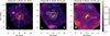 |
Fig. 1 First three channels of MIRI/MRS observations of IRAS 23385+6053. The left panel shows the H2 S(7) transition in channel 1 at 5.511 µm, while the centre and right panels show the averaged continuum in channels 2 and 3. The colour scale in all panels is normalized to the peak intensity. The arrows in the left panel indicate the directions and velocity shift of the major outflows proposed by Beuther et al. (2023). The extraction apertures for our spectra are shown in each panel by the coloured circles. Aperture A+B has a constant radius of 2.5", while all other apertures have aradius that scales with wavelength as r = 2(1.22λ/6.5 m). The grey contours overlaid on channel 2 are 1.3 mm continuum emission (Gieser et al. 2021). The white circle in the bottom left indicates the mean beam size of JWST in the given channel, while the grey ellipse in the second panel indicates the FWHM of the mm beam. |
2.3 Baseline subtraction and ice absorption correction
To characterize the molecular features, we first perform a baseline subtraction using univariate spline fits to line-free regions, in order to remove the thermal continuum, PAH emission, and ice absorption. We also model the thermal continuum using a second order polynomial fit to areas assumed to be free of ice-absorption. Two examples of local baselines and thermal continuum fits to the ~6.5 µm and ~15 µm regions are shown in Fig. A.1. More global continuum fits to study ices are presented in Rocha et al. (2024).
2.4 LTE slab models
We fitted the continuum-subtracted molecular emission using the local thermodynamic equilibrium (LTE) slab models described in Grant et al. (2023), Tabone et al. (2023), which are similar in functionality to the existing slabspec code (Salyk 2020). The molecular emission is assumed to originate in a plane-parallel uniform cylindrical slab of radius R and column density N, with a gas at a single temperature Tex. In reality, proto-stellar environments should contain gas over a wide range of densities and temperatures in the disk, outflow, and envelope which such simple models cannot capture, and non-LTE effects may be particularly important for regions with low density and strong radiative pumping (e.g. outflow shocks). In particular, the effect of mid-IR pumping in particular can result in model excitation temperatures and column densities which do not reflect the kinetic temperature and column density of that gas, which we discuss further in Sect. 4.1. Nevertheless, LTE models are still valuable for identifying and characterizing the molecular emission; we discuss caveats of their use inSect. 4.
The molecular spectroscopy data for the models (transition wavelengths, Einstein A coefficients, statistical weights, and partition functions) are taken from the HITRAN database (Gordon et al. 2022). This information is used in combination with an assumed Tex and N to solve for the level populations. The opacity at line centre is determined assuming a turbulent broadening by a Gaussian with full width at half maximum of ΔV = 4.7 km s−1, which has typically been assumed for LTE models of molecular emission in T Tauri disks (e.g. Salyk et al. 2011). The typical mm line widths in the CORE survey are between 2 and 5 km s−1, so this assumption is reasonable for IRAS 23385+6035 (see Fig. 7 of Cesaroni et al. 2019). The wavelength dependent line optical depth is computed on a high resolution (λ/Δλ) = 106 grid assuming a Gaussian line profile, as there may be significant overlap between closely spaced transitions from molecules with a Q-branch (Tabone et al. 2023). The model flux F(λ) is then computed as
 (1)
(1)
where R is the radius of the emitting slab, d = 4.9 kpc is the distance to the source, Bν is the Planck function, and τ(λ) is the line optical depth. The model is then convolved to the average MIRI instrumental resolution in each sub-band (Labiano et al. 2021; Jones et al. 2023). For comparisons with the observations, we velocity shift the convolved synthetic spectra by vLSR = −50.2 km s−1 for sources A and B (Beuther et al. 2018) and a by-eye-estimated −100 km s−1 for source S1, then finally resample at the observed wavelengths of the MIRI spectra.
Correction for extinction from the local molecular cloud and protostellar envelope is important to obtain accurate column densities from our molecular emission models. We follow the approach of Gieser et al. (2023), who corrected the IRAS 23385+6053 spectra using the extinction curves of McClure (2009) with a K-band extinction of AK = 7.0. However, we make one important modification to more accurately for the effect of ice absorption. The extinction curves of McClure (2009) include features from cloud absorption of H2O and CO2 ice, which may vary significantly from cloud to cloud in shape and depth, and extincts the molecular emission with a strong wavelength dependence. We thus remove the ice features from these extinction curves using a local polynomial fit to ice-free regions. To then include the effect of extinction by ices unique to IRAS 23385+6053 (located in either the protostellar envelope or surrounding molecular cloud), we calculate the optical depth of the ice feature τ = exp (−Fcont/Fbaseline) as a function of wavelength, and apply it as an additional correction factor to our molecular emission models. An example of this correction is shown for CO2 in Fig. A.2, where the ice absorption is seen to significantly weaken the Q and P-branch emission at λ > 14.9 µm. Similarly, from 5.5 to 7.8 µm, there is also strong absorption from H2O,  , and CH4 ice (lower panel of Fig. A.1) which overlaps with the H2O and CH4 emission features, and thus an analogous correction is applied to the models. An important caveat of this approach is the implicit assumption that all of the absorbing ice lies in front of all of the emitting gas. This assumption may not be completely correct if a large fraction of the emitting gas is in an outflow outside the protostellar envelope, and may be further complicated by the presence of multiple sources experiencing varying degrees of extinction within a single aperture in the case of IRAS 23385+6053.
Molecular absorption features are detected in one case (H2O in source B), and modelled in a similar way using LTE slab models based on the work of Helmich (1996). We follow the same procedure outlined above, but only calculating the line optical depth as a function of wavelength, followed immediately by convolution to the MIRI resolution, velocity shifting, and re-sampling. The models are compared to the observed optical depth, which is calculated as τobs = − log(Fobs/Fbaseline). Unlike the case of emission, corrections for extinction by the cloud and envelope ices are not applied, as these do not influence the observed optical depth of the transitions.
Detected molecules.
2.5 Model-fitting procedure
To identify best-fit emission models, for each molecule detected in source A, B, and S1 (see Table 1), we compute a grid of models with varying N and Tex, the details of which are provided in Appendix C. For each model, we calculate
 (2)
(2)
where Fmodel,i· is determined from Eq. (1), σ is estimated from the emission in nearby line-free regions, and a minimization routine is used to determine a value of R that minimizes χ2. The value of σ determined empirically from line-free spectral regions is 0.1 mJy. We only fit regions of the spectrum containing obvious molecular features, thus avoiding contaminating emission from bright atomic lines or other molecules. In some cases, emission from several molecules is blended together (e.g. HCN, OH, C2H2 and CO2, see Grant et al. 2023). Here, we iteratively fit each molecule in order of decreasing flux, using the residuals of the previous best-fit as the input to the following one.
A similar approach is used for identifying best-fit absorption models, but in units of model and observed optical depth, with χ2 calculated as
 (3)
(3)
where τσ = σ/Fobs,i·. We note that in the case of absorption, there is no emitting area radius R to constrain for the ‘pencil-beam’ of the absorbing column.
Uncertainties on the best-fit N and Tex are estimated following Carr & Najita (2011) and Salyk et al. (2011) by producing χ2 maps for the best-fit column density and temperature with contours of the best R value overlaid. Confidence intervals are computed assuming K = 2 degrees of freedom for the column density and temperature following the approach in Avni (1976). Specifically, for the map of  , we overlay contours relative to the best-fit minimum at levels
  . The contour levels corresponding to 1,2, and 3σ are thus
  2.3, 6.2, and 11.8.
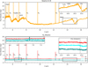 |
Fig. 2 Spectra of sources A+B (top panel) and the brightest H2 knots (lower panel) extracted from the apertures shown in Fig. 1. Flux offsets of −2.5 and −5.0 mJy are applied to the spectra of S2 and S3 respectively. In contrast with the A+B spectrum, no molecular lines other than H2, CO, and OH in S1 are detected towards the H2 knots. |
3 Results
3.1 Detections
An overview of the spectra in the first three MIRI channels is shown in Fig. 2 for the combined A+B aperture (upper panel) and the H2 knots (lower panel). Mid-IR continuum emission is detected towards A + B at a level of up to ~ 10 mJy, orders of magnitude lower than the brighter and more evolved high mass sources studied with ISO (e.g. Boonman et al. 2003a), which cannot be observed by JWST due to rapid saturation of the detectors. No continuum emission is seen at the shock positions S1 to S3. Overlaid on the continuum from A + B are strong absorption features from various silicates and ices (Rocha et al. 2024). The aforementioned H2 S(1) to S(8) transitions as well several shock-tracing ionized atomic lines are detected towards all sources (see Beuther et al. 2023).
A variety of molecular species are detected towards the different sources, which we summarize in Table 1. As previously noted, H2 is detected over the entire MIRI/MRS field of view, and is clearly associated with the outflows (see Gieser et al. 2023). The (0–0) R(6), R(5), and R(4) transitions of HD are detected, which in combination with the H2 lines, will be used as a probe of the D/H abundance in a future publication (Francis et al., in prep.). Strong molecular emission from CO2, C2H2, and HCN is detected towards source A + B (inset, top panel of Figs. 2, 3), as well as fainter ~6 µm and ~16 µm H2O features in the individual sources (Fig. 4). Towards the H2 knots no such features are present (insets, lower panel of Fig. 2), however, emission from CO and OH is detected in source S1 (see also Fig. 5).
The spectra towards source A and B are particularly rich in comparison to the H2 knot positions. In Fig. 3, we show a zoom-in on the A+B spectra in the 13.6–15.6µm range where emission from the CO2, C2H2, and HCN is detected. The CO2 emission is co-located with a strong absorption feature of CO2 ice which extincts the Q- and P-branches of the emission (Sect. 2.4). In both sources, weak emission from OH is detected from 14 to 17 µm, but most transitions except those at ~ 16.04 and ~ 16.84 µm are blended with CO2 and HCN emission. The iso-topologues 13CO2 and 13CCH2 are also detected, but are blended with emission from the P-branch of CO2 and the Q-branch of C2H2.
Several differences are apparent between the spectra of source A and B as well. In channels 1 and 2 (4.9–11.7 µm), emission from sources A and B is spatially resolved, but partial blending and overlap of our extraction apertures begins to occur in channel 3 (11.55–17.98 µm). We therefore analyse source A and B independently in channels 1 and 2 only. In source A, rovi-brational emission from the CO P-branch is detected from 4.9 to 5.2 µm with υ = 1 − 0, J → J + 1 levels up to J = 45 (Eup = 9481 K), indicating extremely energetic excitation conditions. CO emission is entirely absent in source B, however (see Fig. 4).
H2O is detected in both sources from 4.9 to 8 µm in its υ2(1 – 0) vibrational bending mode, but in emission in source A and in absorption in source B. In source A, a handful of ‘cold’ transitions of pure rotational water emission at ~16– 18 µm are also detected, though blending with source B makes this association ambiguous.
In the H2 hotspots, fewer molecules are detected. Emission from CO and OH is only seen towards the brightest source S1 (see Fig. 5), likely tracing the presence of strong, dense shocks.
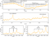 |
Fig. 3 Zoom in on the molecular emission from CO2, C2H2, HCN, and OH emission seen in the A+B aperture (see Fig. 1). No continuum subtraction has been applied. |
3.2 LTE slab model fits
As the emission from CO2 C2H2, HCN, and OH lies in channel 3 where blending between sources A and B is significant, we fitted these species using spectra from the combined A+B aperture.
For all species in channels 1 and 2, we fitted the spectra of source A and B independently. We show an example of the combined best-fit model to source A+B for each molecule in Fig. 6; the fits to the remaining molecules and sources are shown in Figs. B.1–B.3.
For each model, we obtain a best-fit N, Tex, and R, and also calculate the total number of molecules  and a column density ratio with respect to H2. The column densities of H2 for each source have been obtained with a rotational diagram analysis by Gieser et al. (2023). Two temperature components are used in the rotational diagram fitting, and we use the column density of the cooler TTot ~ 300 K H2 for our abundance calculations (see Appendix of Gieser et al. 2023). We note that this is warmer than the best-fit temperatures for CO2, C2H2, and HCN, and cooler than the temperatures for the H2O absorption, and thus the warm H2 may not trace the same reservoir of gas. The H2 emission from IRAS 23385+6053 clearly traces the outflows as well as the protostar positions (see Fig. 1 left panel), and thus our inferred abundances may be higher in reality if only a fraction of the H2 emission originates from the quiescent disk and envelope. However, Gieser et al. (2023) also determine H2 column densities using the mm continuum emission and an assumed gas-to-dust ratio, and find column densities consistent with the warm H2 within a factor of a few. The best-fit parameters of our models and estimated column density ratios are summarized in Table 2.
Confidence interval contours in the N-Tex plane for each fit are overlaid on maps of normalized χ2 in Figs. C.1–C.3. The confidence contours can be complex but typically show one of the following behaviours. 1) The emission is optically thick and the confidence contours are banana-shaped, indicating that R is well-constrained, while N and Tex have a non-linear degeneracy. 2) The emission is optically thin and the confidence contours are tongue-shaped, indicating Tex is well-constrained, but R and N are fully degenerate, and only lower and upper limits respectively can be determined. However, in this case the total number of molecules N is still well-constrained. 3) The S/N of the molecular features is low, resulting in confidence intervals showing a combination of behaviours 1 and 2. Here, solutions with either cooler and more optically thick emission or hotter and more optically thin emission are degenerate.
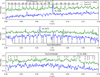 |
Fig. 4 As Fig. 3, but for the CO emission and 4.9–6.7 µm H2O absorption in the spectra of source A (green) and B (blue). |
3.2.1 Source A and B
The high S/N of the CO2 and C2H2 emission allows the parameters of the LTE model fits to be particularly well constrained. For the CO2 emission we fitted only the Q and R-branch. The width of the Q-branch and distribution of the R-branch transitions is particularly sensitive to the excitation temperature in the model fits. We do not fit the P-branch as its S/N is lower and its flux is thus more sensitive to the continuum determination and correction from ice absorption. For C2H2, only the Q-branch is clearly detected and thus used for fitting. The slab model fits for both species indicate optically thick emission, with well-constrained temperatures of 120 ± 10 K and 180 ± 30 K respectively. The best-fit emitting area radii of CO2 ( ) is larger than that of C2H2 (
 ) by a factor of ~13. The emission for HCN has a similar best-fit temperature of ~60 K, but is optically thin and has a poorly constrained emitting area radius of >400 au.
Optically thin emission from the isotopologues 13CO2 and 13CCH2 is tentatively detected, but due to the low S/N of these features, the exact column densities and temperatures cannot be well determined when fit without any constraints. We thus perform the fitting for 13CO2 and 13CCH2 with the model Tex and R fixed to the best-fit values from CO2 and C2H2 respectively, and report the resulting column densities as upper limits. The 13C/12C column density ratio is thus >14 using the CO2 and 13CO2 fits and >9 using the C2H2 and 13CCH2 fits. This ratio is consistent with what is expected from the ISM abundance at a galactocentric distance of 11 kpc of 87 ± 15 from the models of Milam et al. (2005), but higher S/N data is needed to place better constraints on the 13C/12C ratio.
Faint OH emission is detected from both sources and is blended with other molecules except for the groups of transitions at 16.0 and 16.8 micron. The OH emission appears optically thin and has a high Tex of  , as expected from its highly non-LTE formation process (see Sect. 4.5).
For molecules at shorter wavelengths where source A and B can be spatially resolved, there are stark differences between the two spectra. Emission from the P-branch of CO is only detected towards source A. The best-fit solutions suggests optically thin emission with N < 5.6 × 1018 cm−2 and Tex of  , but solutions with optically thick emission and relatively cooler temperatures of 500–1000 K are also plausible at a 2σ level (see Sect. 4.4). H2O is detected in emission from source A but in absorption from source B. The rovibrational emission towards source A is detected at low S/N, and the fitting is further complicated by the difficulty of determining the continuum for such faint features. In Fig. B.1, we thus only show a representative model with a by-eye fit to illustrate the detection. Here, the emitting area radius is set to the best-fit for CO2 of 180 au, a column density of 1014 cm−2, and excitation temperature of 500 K. A handful of pure rotational transitions of H2O in source A are also present at 16–17 µm, though at this wavelength blending with source B is strong. Here, these transitions are consistent with optically thin emission at a temperature of ~350 K but and column densities of < 1018 cm−2. In source B, the absorption model has a best-fit temperature of
  and column density of
  , which is not well constrained due to the low S/N and uncertainty in the continuum determination for H2O transitions deep within ice absorption features.
LTE slab model best-fit parameters.
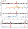 |
Fig. 6 Combined best-fit LTE model for 12CO2, 13CO2, C2H2, 13CCH2, HCN, and OH emission in source A+B (red shaded region) overlaid on the continuum subtracted data with an arbitrary flux offset (black). Prominent emission lines are labelled. Best-fit results for individual molecules are shown as the coloured lines below, with the horizontal bars indicating the regions of spectrum used for fitting. Extinction by CO2 ice has been included in the models, which suppresses the flux from the CO2 gas P-branch (see Sect. 2.4). |
3.2.2 H2 hotspots
In S1, we only detect CO P-branch, OH, and H2 emission. Towards the other H2 hotspots, no other molecular emission is detected. Notably, no CO2 emission is detected, as was seen with ISO Short Wavelength Spectrometer (SWS) towards the Orion-IRC2/KL shock positions (Boonman et al. 2003c). The CO emission appears to be optically thin and consistent with a well-constrained temperature of  . The best-fit emitting radius is larger than a few au, but degenerate with column density. The OH emission has a best-fit solution with ~1300 K optically thick emission, but higher temperatures and an optically thin solution are also possible, as is the case for source A+B.
4 Discussion
Here, we briefly discuss some of the options for the origin of the molecular emission, before discussing each molecule in turn, as they are likely tracing distinct components in IRAS 23385+6053.
4.1 Origin of the emission
Identification of the origin of the emission is complicated by several factors. The spatial resolution of MIRI/MRS at the distance to IRAS 23385+6053 ranges from 1300 to 5000 au, and thus the extraction apertures for our spectra (Fig. 1) may contain emission from a diverse range of environments, including the hot inner disk, warm and colder envelope, irradiated outflow cavity, and gas in outflows with both C and J type shocks. Furthermore, the emission from sources A and B begin to overlap in channel 3, and are entirely blended in channel 4. The fits to source A+B thus indicate the properties of molecular emission in a large region, probably containing at least two disks.
The assumption of LTE at the gas temperature Tkin is likely not appropriate for several of the detected species, as this requires that collisions are the dominant excitation mechanism, and that the density of molecular hydrogen exceeds the critical density for the observed transitions, which are of order 1012 cm−3 for rovibrational transitions (Bruderer et al. 2015). While the typical densities in disks may be large enough for colli-sional excitation, rovibrational molecular emission has also been observed in the much more tenuous gas of protostellar outflows (e.g. Sonnentrucker et al. 2006, 2007; Tappe et al. 2012). Here, radiative pumping from the mid-IR thermal dust continuum or UV emission produced in shocks may instead be responsible for the excitation, and a non-LTE model including these effects would be more appropriate. If mid-IR pumping is the dominant excitation mechanism, the best-fit LTE model temperature may reflect the temperature of the radiation field, which likely originates from the thermal dust continuum. Furthermore, pumping can cause the column density to be overestimated by several orders of magnitude. This effect has recently been identified in observations of SO2 emission from protostars at both mid-IR and sub-mm wavelengths, which confirm the presence of strong mid-IR pumping (van Gelder et al. 2024). However, in general the strength and shape of the local radiation fields are highly uncertain, and depend on the local extinction and source geometry. Even if molecular emission does originate in the disk, large gradients in temperature and density should be present, and the assumption of a single temperature may not be valid. Nonetheless, the LTE slab models provide a good fit to the observations, except for the case of H2O. We discuss in the following sections the case of each molecule in detail, and note where non-LTE effects may be important.
4.2 Simple organics – CO2, C2H2, HCN
Emission from the simple organic molecules CO2, C2H2, and HCN has often been detected in absorption towards high mass protostars in the hot core phase (e.g Lahuis & van Dishoeck 2000; Boonman et al. 2003c; Barr et al. 2020). However, IRAS 23385+6053 is likely in an earlier stage of evolution, as indicated by the lack of a compact HII region or free-free emission (Molinari et al. 1998), and the low number of detected COMs associated with high temperature chemistry and ice sublimation (Cesaroni et al. 2019; Gieser et al. 2021). The general lack of absorption, which requires colder absorbing gas in front of a warm continuum along the line of sight, is thus not surprising. The similar temperatures (100–200 K) and emitting areas (10s to 100s of au) of the LTE model fits suggest a common origin for the simple organics. For source A+B, the CO2 and C2H2 emission is optically thick while the HCN emission is optically thin, which is consistent with models that predict the strongest HCN transitions become optically thick at about an order of magnitude higher column density than C2H2 (Lahuis & van Dishoeck 2000).
The simple organics may be tracing a variety of components of a young protostellar system. Previous Spitzer observations of protostars have found emission from these species to be associated with the outflows. In Spitzer Infrared Spectrograph observations of the Cepheus A star-forming region (d = 690 pc), Sonnentrucker et al. (2006, 2007) found spatially extended (~21 000 au) CO2 and C2H2 emission with temperatures of 50–200 K and column densities of 1017 to 1019 cm−2. In the Orion-IRc2/KL (d ~ 450 pc) region, Boonman et al. (2003c) similarly detected CO2, C2H2, and HCN emission from H2 bright shocked regions. In both cases, the low densities of the outflow regions relative to the critical densities of the simple organics supported mid-IR pumping by the local dust as the dominant excitation mechanism for the observed emission. However, while Sonnentrucker et al. (2006, 2007) find a strong correlation between the spatial extent of the simple organics and extended H2 emission, in IRAS 23385+6053 these molecules are only detected towards source A and B, have emitting area radii < 200 au, and are not seen at the outflow knot positions (cf. Fig. 2 and Table 1). This would suggest that the simple organics do not primarily originate in the shocks, and are instead more likely to be associated with a protostellar disk and/or dense inner envelope. The prior detection towards source A of large scale gas motions resembling combined keplerian rotation and infall onto a nearly face on disk supports the disk scenario (Cesaroni et al. 2019).
The large emitting area radii (> 10s of au), temperatures of 100–200 K, and lack of strong water emission argues against the emission arising from the hot inner disk, as has typically been found in the more evolved T Tauris objects (Carr & Najita 2011). Instead, the emission may come from the extended warm disk surface and dense inner envelope that would be expected around young high mass protostars. The emitting radius for CO2 of ~ 180 au is much larger than a typical T Tauri star disk, but is consistent with interferometric observations of high mass protostars that suggest disks of hundreds to thousands of au in radius (e.g. Johnston et al. 2015; Maud et al. 2019). Models of high-mass embedded disks by Nazari et al. (2022, see also van Dishoeck et al. 2023) indeed show typical temperatures of 150–200 K at radii of ~100–200 au. The dense environment of the disk should exceed the critical densities of the simple organic molecules, and in this case the assumption of LTE may be reasonable. However, we cannot rule out a contribution from mid-IR pumping from the dust in the disk or outflows. The lack of mid-IR continuum emission towards the H2 knot positions suggests that pumping would only be important close to source A and B, but more modelling of the location radiation field is required to evaluate this scenario fully and is beyond the scope of this paper.
4.3 H2O
Similar to the case of the simple organics, H2O is likely not associated with large scale molecular outflows, as the emission and absorption is only detected towards sources A and B, and none of the H2 knot positions (cf. Fig. 2 and Table 1). This is in stark contrast to the ubiquitous detection of H2O far-IR and sub-mm lines in shocks and outflows (van Dishoeck et al. 2021). Mid-IR H2O emission in protostars has not been well characterized previously owing to the relative lack of sensitivity of previous space missions compared to JWST. In the low mass protostars of the Spitzer c2d survey, H2O emission was rarely detected (12/43 sources), and for all but one source, only in the more evolved class I stage (Lahuis et al. 2010). For these more evolved sources, the H2O emission appeared to have similar properties to class II disks, with hot temperatures and small emitting radii. In the sole mid-IR detection towards a class 0 source, the H2O emission appeared cold (Tex ~ 170 K) and was suggested to originate from an accretion shock onto the disk (Watson et al. 2007), although this was later disputed by an analysis of far-IR H2O emission with Herschel Herczeg et al. (2012). In source A, the parameters of the H2O emission are not well determined, but the temperature of our representative model of ~500 K would be consistent with an origin in the disk surface.
In previous observations of high mass protostars, H2O has typically been detected in absorption (Boonman et al. 2003a; Boonman & van Dishoeck 2003; Indriolo et al. 2020; Barr et al. 2022). Two non-mutually-exclusive possible scenarios involve a disk origin of the absorption and have been proposed for previous observations of protostars. In the first, absorption occurs in the disk atmosphere against the continuum from the midplane, which is viscously heated by accretion (e.g Barr et al. 2022). In the second, the disk is viewed nearly edge on relative to the observer, and the absorption occurs against the continuum from the hot inner disk on a line of sight intersecting the disk (e.g., Lahuis et al. 2006; Knez et al. 2009). A difference in inclination is an attractive possibility for explaining why we see H2O in emission in source A but in absorption in source B. However, a nearly edge-on disk would also be expected to produce strong absorption features from CO2, C2H2, and HCN which we do not detect (Lahuis et al. 2006; Knez et al. 2009). A third possibility is that the H2O absorption originates in a dense inner disk wind against the continuum from the disk, but this may require a very specific inclination angle of the disk which matches the opening angle of the wind. We propose that the most likely scenario is that the disks in source A and B are both viewed at a low to moderate inclination, but that the viscous heating of the mid-plane is stronger in source B due to a much higher accretion rate, resulting in absorption. In source A, the weak H2O emission then traces the warm inner disk, similar to what has been observed for class II disks (Carr & Najita 2011).
4.4 CO
In MIRI/MRS observations, the detection of any CO emission indicates highly energetic excitation conditions, as the shortest wavelength cutoff of 4.9 µm limits us to the detection of P-branch transitions with high upper energy levels (Eup > 4600 K, Jup > 24). The best-fit LTE CO models for source A and source S1 appear to indicate optically thin emission with high temperatures T > 1900 K. However, even with the simplifying assumption of LTE, it may not be possible to robustly determine the gas temperature due to the combination of optical depth effects and the lack of lower energy transitions (Herczeg et al. 2011). To illustrate this, we show in Fig. 7 synthetic rotational diagrams of the CO υ = 1 − 0 P-branch produced using a 1000 K LTE slab model at a variety of column densities, with the optical depth of each line indicated by the colour scale. At Eup ≳ 4600 K (dotted line), the υ = 1 − 0 P-branch transitions lie within the MIRI/MRS range at λ > 4.9 µm. A linear fit to the MIRI/MRS range transitions recovers the true temperature of 1000 K for a very optically thin model (N = 1017 cm−2), but is increasingly biased towards higher temperatures as the emission becomes optically thick. While our LTE models can account for optical depth effects, the curvature in the rotational diagram is only easily recognized in the lower upper-energy transitions located at < 4.9 µm. This effect similarly holds for the υ = 2 − 1 P-branch transitions in the MIRI range, which have even higher upper energy levels of > 7000 K. Observations with instruments covering shorter wavelengths (e.g. JWST/NIRSpec or VLT/CRIRES+) are therefore required for accurate modelling.
With this in mind, we can only conclude reliably that the observed CO emission in sources A and S1 originates from gas with a high excitation temperature, T ≳ 1000 K. What could explain this CO emission (and the non-detection of CO emission in source B)? CO rovibrational emission from protostars has been studied in detail from ground based high spectral resolution observations. Analysis of the emission line velocity profiles typically indicates that the emission originates from a broad and hot component (T ~ 1000 K) in the inner edge of the disk – similar to what is commonly observed for Class II disks (Salyk et al. 2011) – or within a narrow and cooler (T ~ 300 K), component associated with a disk wind or outflow shocks (Pontoppidan et al. 2002; Herczeg et al. 2011). Assuming that LTE holds, an inner disk-origin of the CO emission seems most reasonable for source A, and would be consistent with the other molecule detections. However, CO can be significantly pumped by strong mid-IR radiation (Blake & Boogert 2004; Thi et al. 2001), and an outflow origin cannot be ruled out. An outflow origin is more likely the case for the H2 knot in source S1. Here, strong outflow activity is suggested by the high H2 line velocities, but we do not detect mid-IR continuum emission, nor any of the H2O or simple organics seen towards source A B that suggest a disk. For source B, the reason for the non-detection of CO is unclear, as a disk is likely present given the significant H2O absorption, and there is significant outflow activity within this aperture as well. High spectral resolution studies of CO have shown that the line profiles for some sources can show a complex velocity structure with a combination of emission and absorption from the disk and disk winds (Herczeg et al. 2011; Thi et al. 2010). At low spectral resolution, blending of these features may smooth out the line profiles to a very low flux, making the CO difficult to detect. This scenario would be more likely if the H2O absorption indeed originates from a disk wind. Alternatively, the emitting region for CO may be much smaller in source B, and thus the emission would simply be below our detection threshold.
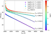 |
Fig. 7 Rotational diagrams of CO υ = 1 − 0 P-branch transitions produced using our LTE slab model for four different column densities at a temperature of T = 1000 K; the colour of each symbol indicates the line optical depth. The dotted line at Eup = 4600 K is the energy above which transitions fall shortwards of the MIRI/MRS blue wavelength limit of 4.9 µm. For each model, the rotational temperature derived from a linear fit to transitions in the MIRI range (i.e. above Eup = 4600 K) is shown by the black lines. |
4.5 OH
The OH transitions detected towards sources A+B and S1 are best fit by optically thin LTE models with high excitation temperatures of Tex > 1300 K. However, the detected transitions from 13 to 17 µm have very high upper levels (Euv ~ 8000–10 000 K, N = 21–17) as well as large Einstein A coefficients (Aij ~ 100 s−1), indicating that collisional excitation is not plausible as an excitation mechanism and that strong non-LTE processes are at play. Mid-IR OH emission has previously been detected in environments with strong UV irradiation, such as shocks from protostellar outflows (Tappe et al. 2008, 2012) and the surface layers of class II disks (Carr & Najita 2014). Here, OH transitions in extremely high rotational states (Eup ~ 40 000 K) but low lying vibrational states are observed. These transitions can be explained by the photodissociation of H2O by UV photons in the  absorption band, which produces OH in extremely hot rotational states, followed by ‘prompt’ emission of photons associated with a cascade of pure rotational transitions to the ground state (Tabone et al. 2021; Zannese et al. 2023). However, these prompt transitions lie primarily at 9–11 µm and are not detected in our observations. Furthermore, the rotational lines of OH are split into a quadruplet by spin-orbit coupling and Λ-doubling, and for prompt OH emission, a strong asymmetry is expected between the components, but we do not observe this (Tabone et al., in prep.). A different non-LTE mechanism is the formation pumping of OH to highly excited rotational and vibrational states as the result of the O + H2 → OH + H reaction (Liu et al. 2000), which can produce the emission long-wards of ~13 µm we observe. Further non-LTE modelling is required to understand the excitation mechanism, but is beyond the scope of this paper. The lack of detection of OH towards the H2 knots S2 and S3 could be explained by weaker shock activity at these locations, resulting in OH emission below our detection limits.
4.6 Chemistry
Here, we comment on the chemistry for the simple organics CO2, C2H2, and HCN, which have relatively precise LTE model fits. We caution that if significant mid-IR pumping is present, this would bias our LTE model fits towards higher column densities and abundances than are actually observed, and the excitation temperature would reflect the temperature of the radiation field rather than the kinetic temperature of the gas. The H2 column densities used for our abundance determination also likely traces gas in the outflows as well as the disk and envelope, which would bias out abundances towards lower values.
We proceed here assuming that emission from these molecules originates in the disk and is indeed in LTE. What then is the origin of the molecules themselves? The presence of deep CO2 ice absorption features at ~14.9 µm clearly indicates the presence of abundant CO2 on the grain mantles along the line of sight in the larger scale envelopes. The dust temperature towards sources A and B estimated from a black-body fit of ~150 K exceeds the sublimation temperature of CO2 of ~55 K, indicating thermal desorption closer to the protostars. The detection of [FeII], [SI] towards source A and B (Gieser et al. 2023) implies strong shocks capable of sputtering ices from the grain mantle are also present. Either or both mechanisms could release CO2 into the gas phase, and a similar scenario could apply for the C2H2 and HCN emission, although both of these molecules have yet to be detected in ices.
Gas-phase chemistry may also contribute to the formation of the observed molecules. This may particularly be likely for CO2, which has enhanced production by the reaction OH + CO → CO2 + H at temperatures of 100–250 K. Above this temperature range, Oxygen is instead driven into H2O by OH + H2 → H2O + H, and CO2 enhancement is not expected (van Dishoeck et al. 2023). For HCN and C2H2, gas phase production can occur efficiently at temperatures >200 K via the CN + H2 → HCN + H reaction for HCN, and through multiple pathways for C2H2 (Doty et al. 2002). However, our LTE model fits find excitation temperatures < 200 K for both molecules, suggesting that gas phase formation is not important.
In the context of hot core observations of gas-phase absorption, the abundance of C2H2 and HCN has been found to be correlated with Tex (Lahuis & van Dishoeck 2000), while CO2 shows no such trends (Boonman et al. 2003b). The abundance of HCN is only constrained by our modelling to <10–5, but C2H2 and CO2 abundances of ~10−7 are consistent with hot cores with Tex ~ 200 K. The hot core chemistry models of Lahuis et al. (2007) provide predictions for the CO2, C2H2, and HCN abundance over a range of excitation temperatures and X-ray fluxes. Comparing our CO2 model fit results with Fig. 3 of Lahuis et al. (2007), at a Tex of ~120 K the CO2 abundance is very sensitive to X-ray flux. However, our best-fit abundance of ~2 × 10⁻⁷ is possible for some models with lower X-ray flux (<1 erg s−1 cm−2). For C2H2 at ~180 K, very low abundances of <10−9 are expected, but we have ~3 × 10⁻⁷. Deeper JWST searches for both HCN and C2H2 ices are warranted, which could mitigate the C2H2 discrepancy.
5 Summary and future outlook
In Fig. 8, we summarize the proposed origins of the different molecular emission components observed towards IRAS 23385+6053. Taken together, the detected molecular species are largely consistent with an origin in a young disk and inner envelope, with a possible contribution from a dense inner disk wind. The major caveats to this picture are the limited spatial resolution at the large distance to the source, and the possibility of non-LTE effects, which we discuss in Sect. 4.1. With this in mind, the interpretation of our models is as follows:
In the blended spectrum from source A+B, warm 120–180 K emission of CO2, C2H2, and HCN is seen. The origin is most likely predominantly in the warm disk surface or dense inner envelope, but some contribution from the base of an outflow within the JWST beam cannot be ruled out. These species are not detected towards the shock positions in source S1–S3;
H2O is only detected towards source A and B, and not towards any shock positions, suggesting a disk rather than a large scale outflow origin. In source B, strong accretion heating in the disk midplane can produce a temperature inversion, resulting in hot 250–1050 K H2O absorption. Alternatively, the absorption may occur in a dense inner disk wind, though this requires a very specific geometry. In source A, the accretion heating is weaker, and some faint H2O emission is detected, which may originate in the inner disk.
CO tracing an inner disk and/or outflow shocks is detected towards source A and S1. Only high-J P-branch states are detectable in the MIRI/MRS range of 4.9 – 28.3 µm, which suggests high temperatures T > 1000 K. Observations at shorter wavelengths covering the lower J lines are needed to determine the temperature if the emission is optically thick. CO is not detected towards source B, possibly due to absorption in a disk wind being filled in by emission from the disk;
Highly non-LTE OH emission is detected towards source A, B, and S1, but not S2 or S3. Photo-dissociation or chemical formation pumping is likely responsible for the emission in high rotational states observed, although we do not detect the prompt OH transitions at 9–11 µm or Λ-doublet asymmetry associated with photo-dissociation.
There are many opportunities for complementary observations and modelling to improve the exploitation of MIRI/MRS data. For complex and distant high mass star-forming regions, spatial resolution is still a limiting factor. Long-baseline observations with ALMA can approach the scale of the disk, though these are not possible for IRAS 23385+6053 given its high latitude relative to the ALMA observatory. At shorter wavelengths, ground based observations of CO and H2 O with high spectral resolution can provide valuable kinematic information for distinguishing between a disk and outflow origin, although sources like IRAS 23385+6053 are too faint for 8m class telescopes. Observations with JWST/NIRSpec would capture the full CO rovibrational band and a variety of accretion tracing HI lines accessible in the near-IR. On the modelling front, non-LTE analysis will be important for molecular emission detected in the high energy and low density environments of protostellar outflows. In particular, analysis of prompt OH emission produced by photo-dissociation of H2O can provide valuable insights into the local UV fields and density of H2O.
The unprecedented sensitivity of JWST is opening a new window into high mass star formation allowing extremely faint and distant sources to be detected and characterized for the first time. With the imminent arrival of additional MIRI/MRS observations of high mass protostars, our understanding of how a very young object such as IRAS 23385+6053 fits into the broader evolution will greatly improve.
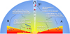 |
Fig. 8 Schematic of our proposed origins for the molecular emission and absorption observed towards source A (right half), B (left half), and S1 (outflow shocks, centre) in IRAS 23385+6053. |
Acknowledgements
We would like to thank the anonymous referee for their very constructive discussions on this paper. This work is based on observations made with the NASA/ESA/CSA James Webb Space Telescope. The data were obtained from the Mikulski Archive for Space Telescopes at the Space Telescope Science Institute, which is operated by the Association of Universities for Research in Astronomy, Inc., under NASA contract NAS 5-03127 for JWST. These observations are associated with programme 1290. Astrochemistry in Leiden is supported by funding from the European Research Council (ERC) under the European Union’s Horizon 2020 research and innovation program-meme (grant agreement no. 101019751 MOLDISK), by the Netherlands Research School for Astronomy (NOVA), and by grant TOP-1 614.001.751 from the Dutch Research Council (NWO).
Appendix A Thermal continuum and baseline modelling
Here, we show examples of the local continuum modelling procedure applied to our data and additional extinction corrections applied to our gas-phase emission models. In Figure A.1, examples of cubic spline fits to the local continuum at shown by the black points and solid lines overlaid on the data for source A in green. Additionally, the thermal dust continuum estimated with a cubic spline fit (dashed line) to the red data points is indicated. These estimates of the thermal dust continuum are used to calculate the wavelength dependent extinction of the ice features τice = − log(Fdust/Fcontinuum). The wavelength dependent extinction is applied as a correction factor exp(−τice) to our LTE models for emission from molecular species overlapping with the ice features, as demonstrated in Figure A.2 for the gas of gas-phase CO2. The effect in this case is to suppress the emission from the Q– and P– branch.
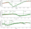 |
Fig. A.1 Example of local continuum spline fitting and modelling of the CO2 (top panel), H2O (middle panel), and |

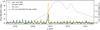 |
Fig. A.2 Correction for differential extinction by CO2 ice of the CO2 gas emission features. The blue line shows the continuum subtracted data with the CO2 ice feature removed. The best-fit LTE model of CO2 with extinction correction, but without any correction for ice absorption (orange) overproduces the Q and P-branch emission. The estimated optical depth of the CO2 ice feature (dashed grey line) is applied as a scaling factor to the same best-fit model (green curve), which significantly improves the fit to the Q-branch, though the P-branch features are now somewhat under-produced. |
Appendix B Model fits
In this section, we show the best-fit LTE models for each molecule in the same manner as Figure 6. In Figures, B.1, B.2, and B.3, the LTE model for each fit is shown by the coloured lines, and compared to the continuum-subtracted data (black) in the overlaid red-shaded region.
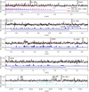 |
Fig. B.1 As Figure 6, but for the best-fit LTE models of CO, H2O emission at 5.5–7.7 µm and 16–18 µm in source A. |
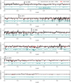 |
Fig. B.3 As Figure 6, but the observed data for source B is shown in units of optical depth with an offset of −0.5 relative to the best-fit LTE model for H2O absorption. |
Appendix C LTE model χ2 maps
The resolution of the LTE model grids used to fit our observations are the same in column density, but vary in temperature depending on the S/N of the emission and excitation conditions. For all species, the column density range is N = 1014 –1024 cm−2 in steps of log(N) = 0.166. For the relatively high S/N emission from cold CO2, HCN, and C2H2, the temperature range is T = 10 – 500 K in steps of 10 K. For the highly excited emission from CO and OH, a range of T = 10 – 500 K in steps of 67 K is used. For all other species, the the temperature in the grid ranges from T = 25 – 1500 in steps of 25K. Our LTE model fits are shown for source A+B in Figure C.1, for source A and B separately in Figure C.2, and for source S1 in Figure C.3.
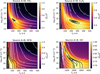 |
Fig. C.1 Normalized χ2 maps (colour scale) of the LTE model temperature and column density grids for CO2, C2H2, HCN, and OH model fits in source A+B. The best-fit emitting radius for each model is overlaid as white contours, while the 1, 2, and 3 σ confidence interval contours are overlaid in black. The best-fit model at the minimum χ2 is shown by a blue cross. |
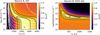 |
Fig. C.2 As Figure C.1, but for CO emission in source A and H2O absorption in source B |
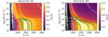 |
Fig. C.3 As Figure C.1, but for CO and OH emission in source S1. |
References
- Argyriou, I., Glasse, A., Law, D. R., et al. 2023, A&A, 675, A111 [NASA ADS] [CrossRef] [EDP Sciences] [Google Scholar]
- Avni, Y. 1976, ApJ, 210, 642 [NASA ADS] [CrossRef] [Google Scholar]
- Banzatti, A., Abernathy, K. M., Brittain, S., et al. 2022, AJ, 163, 174 [NASA ADS] [CrossRef] [Google Scholar]
- Banzatti, A., Pontoppidan, K. M., Pére Chávez, J., et al. 2023, AJ, 165, 72 [CrossRef] [Google Scholar]
- Barr, A. G., Boogert, A., DeWitt, C. N., et al. 2020, ApJ, 900, 104 [NASA ADS] [CrossRef] [Google Scholar]
- Barr, A. G., Boogert, A., Li, J., et al. 2022, ApJ, 935, 165 [NASA ADS] [CrossRef] [Google Scholar]
- Beuther, H., Mottram, J. C., Ahmadi, A., et al. 2018, A&A, 617, A100 [NASA ADS] [CrossRef] [EDP Sciences] [Google Scholar]
- Beuther, H., van Dishoeck, E. F., Tychoniec, L., et al. 2023, A&A, 673, A121 [NASA ADS] [CrossRef] [EDP Sciences] [Google Scholar]
- Blake, G. A., & Boogert, A. C. A. 2004, ApJ, 606, L73 [NASA ADS] [CrossRef] [Google Scholar]
- Boonman, A. M. S., & van Dishoeck, E. F. 2003, A&A, 403, 1003 [NASA ADS] [CrossRef] [EDP Sciences] [Google Scholar]
- Boonman, A. M. S., Doty, S. D., van Dishoeck, E. F., et al. 2003a, A&A, 406, 937 [NASA ADS] [CrossRef] [EDP Sciences] [Google Scholar]
- Boonman, A. M. S., van Dishoeck, E. F., Lahuis, F., & Doty, S. D. 2003b, A&A, 399, 1063 [NASA ADS] [CrossRef] [EDP Sciences] [Google Scholar]
- Boonman, A. M. S., van Dishoeck, E. F., Lahuis, F., et al. 2003c, A&A, 399, 1047 [NASA ADS] [CrossRef] [EDP Sciences] [Google Scholar]
- Bruderer, S., Harsono, D., & van Dishoeck, E. F. 2015, A&A, 575, A94 [NASA ADS] [CrossRef] [EDP Sciences] [Google Scholar]
- Bushouse, H., Eisenhamer, J., Dencheva, N., et al. 2022, https://doi.org/10.5281/zenodo.6984366 [Google Scholar]
- Carr, J. S., & Najita, J. R. 2008, Science, 319, 1504 [Google Scholar]
- Carr, J. S., & Najita, J. R. 2011, ApJ, 733, 102 [NASA ADS] [CrossRef] [Google Scholar]
- Carr, J. S., & Najita, J. R. 2014, ApJ, 788, 66 [NASA ADS] [CrossRef] [Google Scholar]
- Cesaroni, R., Felli, M., Testi, L., Walmsley, C. M., & Olmi, L. 1997, A&A, 325, 725 [NASA ADS] [Google Scholar]
- Cesaroni, R., Beuther, H., Ahmadi, A., et al. 2019, A&A, 627, A68 [EDP Sciences] [Google Scholar]
- Doty, S. D., van Dishoeck, E. F., van der Tak, F. F. S., & Boonman, A. M. S. 2002, A&A, 389, 446 [NASA ADS] [CrossRef] [EDP Sciences] [Google Scholar]
- Evans, Neal J., I., Lacy, J. H., & Carr, J. S. 1991, ApJ, 383, 674 [NASA ADS] [CrossRef] [Google Scholar]
- Fontani, F., Cesaroni, R., Testi, L., et al. 2004, A&A, 414, 299 [NASA ADS] [CrossRef] [EDP Sciences] [Google Scholar]
- Gasman, D., van Dishoeck, E. F., Grant, S. L., et al. 2023, A&A, 679, A117 [NASA ADS] [CrossRef] [EDP Sciences] [Google Scholar]
- Gerner, T., Beuther, H., Semenov, D., et al. 2014, A&A, 563, A97 [NASA ADS] [CrossRef] [EDP Sciences] [Google Scholar]
- Gieser, C., Beuther, H., Semenov, D., et al. 2021, A&A, 648, A66 [EDP Sciences] [Google Scholar]
- Gieser, C., Beuther, H., van Dishoeck, E. F., et al. 2023, A&A, 679, A108 [NASA ADS] [CrossRef] [EDP Sciences] [Google Scholar]
- Gordon, I. E., Rothman, L. S., Hargreaves, R. J., et al. 2022, J. Quant. Spec. Radiat. Transf., 277, 107949 [NASA ADS] [CrossRef] [Google Scholar]
- Grant, S. L., van Dishoeck, E. F., Tabone, B., et al. 2023, ApJ, 947, L6 [NASA ADS] [CrossRef] [Google Scholar]
- Greenfield, P., & Miller, T. 2016, Astron. Comput., 16, 41 [NASA ADS] [Google Scholar]
- Helmich, F. P. 1996, PhD thesis, Leiden University, The Netherlands [Google Scholar]
- Helmich, F. P., van Dishoeck, E. F., Black, J. H., et al. 1996, A&A, 315, L173 [NASA ADS] [Google Scholar]
- Herczeg, G. J., Brown, J. M., van Dishoeck, E. F., & Pontoppidan, K. M. 2011, A&A, 533, A112 [NASA ADS] [CrossRef] [EDP Sciences] [Google Scholar]
- Herczeg, G. J., Karska, A., Bruderer, S., et al. 2012, A&A, 540, A84 [NASA ADS] [CrossRef] [EDP Sciences] [Google Scholar]
- Hollenbach, D., & McKee, C. F. 1989, ApJ, 342, 306 [Google Scholar]
- Indriolo, N., Neufeld, D. A., Barr, A. G., et al. 2020, ApJ, 894, 107 [NASA ADS] [CrossRef] [Google Scholar]
- Johnston, K. G., Robitaille, T. P., Beuther, H., et al. 2015, ApJ, 813, L19 [Google Scholar]
- Jones, O. C., Álvarez-Márquez, J., Sloan, G. C., et al. 2023, MNRAS, 523, 2519 [Google Scholar]
- Knez, C., Lacy, J. H., Evans, Neal J. I., van Dishoeck, E. F., & Richter, M. J. 2009, ApJ, 696, 471 [NASA ADS] [CrossRef] [Google Scholar]
- Kóspál, Á., Ábrahám, P., Diehl, L., et al. 2023, ApJ, 945, L7 [CrossRef] [Google Scholar]
- Labiano, A., Argyriou, I., Álvarez-Márquez, J., et al. 2021, A&A, 656, A57 [NASA ADS] [CrossRef] [EDP Sciences] [Google Scholar]
- Lahuis, F., & van Dishoeck, E. F. 2000, A&A, 355, 699 [NASA ADS] [Google Scholar]
- Lahuis, F., van Dishoeck, E. F., Boogert, A. C. A., et al. 2006, ApJ, 636, L145 [NASA ADS] [CrossRef] [Google Scholar]
- Lahuis, F., Spoon, H. W. W., Tielens, A. G. G. M., et al. 2007, ApJ, 659, 296 [Google Scholar]
- Lahuis, F., van Dishoeck, E. F., Jørgensen, J. K., Blake, G. A., & Evans, N. J. 2010, A&A, 519, A3 [NASA ADS] [CrossRef] [EDP Sciences] [Google Scholar]
- Law, D. R., E. Morrison, J., Argyriou, I., et al. 2023, AJ, 166, 45 [NASA ADS] [CrossRef] [Google Scholar]
- Liu, X., Lin, J. J., Harich, S., Schatz, G. C., & Yang, X. 2000, Science, 289, 1536 [CrossRef] [Google Scholar]
- Maud, L. T., Cesaroni, R., Kumar, M. S. N., et al. 2019, A&A, 627, L6 [NASA ADS] [CrossRef] [EDP Sciences] [Google Scholar]
- McClure, M. 2009, ApJ, 693, L81 [NASA ADS] [CrossRef] [Google Scholar]
- Milam, S. N., Savage, C., Brewster, M. A., Ziurys, L. M., & Wyckoff, S. 2005, ApJ, 634, 1126 [Google Scholar]
- Molinari, S., Testi, L., Brand, J., Cesaroni, R., & Palla, F. 1998, ApJ, 505, L39 [NASA ADS] [CrossRef] [Google Scholar]
- Motte, F., Bontemps, S., & Louvet, F. 2018, ARA&A, 56, 41 [NASA ADS] [CrossRef] [Google Scholar]
- Mottram, J. C., Hoare, M. G., Davies, B., et al. 2011, ApJ, 730, L33 [Google Scholar]
- Nazari, P., Tabone, B., Rosotti, G. P., et al. 2022, A&A, 663, A58 [NASA ADS] [CrossRef] [EDP Sciences] [Google Scholar]
- Perotti, G., Christiaens, V., Henning, T., et al. 2023, Nature, 620, 516 [NASA ADS] [CrossRef] [Google Scholar]
- Pontoppidan, K. M., Schöier, F. L., van Dishoeck, E. F., & Dartois, E. 2002, A&A, 393, 585 [NASA ADS] [CrossRef] [EDP Sciences] [Google Scholar]
- Pontoppidan, K. M., Salyk, C., Blake, G. A., & Käufl, H. U. 2010, ApJ, 722, L173 [NASA ADS] [CrossRef] [Google Scholar]
- Pontoppidan, K. M., Salyk, C., Bergin, E. A., et al. 2014, in Protostars and Planets VI, eds. H. Beuther, R. S. Klessen, C. P. Dullemond, & T. Henning, 363 [Google Scholar]
- Rieke, G. H., Wright, G. S., Böker, T., et al. 2015, PASP, 127, 584 [NASA ADS] [CrossRef] [Google Scholar]
- Rocha, W. R. M., van Dishoeck, E. F., Ressler, M. E., et al. 2024, A&A, 683, A124 [NASA ADS] [CrossRef] [EDP Sciences] [Google Scholar]
- Salyk, C. 2020, https://doi.org/10.5281/zenodo.4037306 [Google Scholar]
- Salyk, C., Pontoppidan, K. M., Blake, G. A., Najita, J. R., & Carr, J. S. 2011, ApJ, 731, 130 [Google Scholar]
- Sonnentrucker, P., González-Alfonso, E., Neufeld, D. A., et al. 2006, ApJ, 650, L71 [CrossRef] [Google Scholar]
- Sonnentrucker, P., González-Alfonso, E., & Neufeld, D. A. 2007, ApJ, 671, L37 [NASA ADS] [CrossRef] [Google Scholar]
- Tabone, B., van Hemert, M. C., van Dishoeck, E. F., & Black, J. H. 2021, A&A, 650, A192 [NASA ADS] [CrossRef] [EDP Sciences] [Google Scholar]
- Tabone, B., Bettoni, G., van Dishoeck, E. F., et al. 2023, Nat. Astron., 7, 805 [NASA ADS] [CrossRef] [Google Scholar]
- Tappe, A., Lada, C. J., Black, J. H., & Muench, A. A. 2008, ApJ, 680, L117 [Google Scholar]
- Tappe, A., Forbrich, J., Martín, S., Yuan, Y., & Lada, C. J. 2012, ApJ, 751, 9 [NASA ADS] [CrossRef] [Google Scholar]
- Thi, W. F., van Dishoeck, E. F., Blake, G. A., et al. 2001, ApJ, 561, 1074 [CrossRef] [Google Scholar]
- Thi, W. F., van Dishoeck, E. F., Pontoppidan, K. M., & Dartois, E. 2010, MNRAS, 406, 1409 [Google Scholar]
- van Dishoeck, E. F. 2004, ARA&A, 42, 119 [NASA ADS] [CrossRef] [Google Scholar]
- van Dishoeck, E. F., Kristensen, L. E., Mottram, J. C., et al. 2021, A&A, 648, A24 [NASA ADS] [CrossRef] [EDP Sciences] [Google Scholar]
- van Dishoeck, E. F., Grant, S., Tabone, B., et al. 2023, Faraday Discuss, 245, 52 [NASA ADS] [CrossRef] [Google Scholar]
- van Gelder, M. L., Ressler, M. E., van Dishoeck, E. F., et al. 2024, A&A, 682, A78 [NASA ADS] [CrossRef] [EDP Sciences] [Google Scholar]
- Watson, D. M., Bohac, C. J., Hull, C., et al. 2007, Nature, 448, 1026 [NASA ADS] [CrossRef] [Google Scholar]
- Wells, M., Pel, J. W., Glasse, A., et al. 2015, PASP, 127, 646 [NASA ADS] [CrossRef] [Google Scholar]
- Wright, G. S., Wright, D., Goodson, G. B., et al. 2015, PASP, 127, 595 [NASA ADS] [CrossRef] [Google Scholar]
- Wright, G. S., Rieke, G. H., Glasse, A., et al. 2023, PASP, 135, 048003 [NASA ADS] [CrossRef] [Google Scholar]
- Yang, Y.-L., Green, J. D., Pontoppidan, K. M., et al. 2022, ApJ, 941, L13 [NASA ADS] [CrossRef] [Google Scholar]
- Zannese, M., Tabone, B., Habart, E., et al. 2023, A&A, 671, A41 [NASA ADS] [CrossRef] [EDP Sciences] [Google Scholar]
All Tables
All Figures
|
Fig. 1 First three channels of MIRI/MRS observations of IRAS 23385+6053. The left panel shows the H2 S(7) transition in channel 1 at 5.511 µm, while the centre and right panels show the averaged continuum in channels 2 and 3. The colour scale in all panels is normalized to the peak intensity. The arrows in the left panel indicate the directions and velocity shift of the major outflows proposed by Beuther et al. (2023). The extraction apertures for our spectra are shown in each panel by the coloured circles. Aperture A+B has a constant radius of 2.5", while all other apertures have aradius that scales with wavelength as r = 2(1.22λ/6.5 m). The grey contours overlaid on channel 2 are 1.3 mm continuum emission (Gieser et al. 2021). The white circle in the bottom left indicates the mean beam size of JWST in the given channel, while the grey ellipse in the second panel indicates the FWHM of the mm beam. |
| In the text | |
|
Fig. 2 Spectra of sources A+B (top panel) and the brightest H2 knots (lower panel) extracted from the apertures shown in Fig. 1. Flux offsets of −2.5 and −5.0 mJy are applied to the spectra of S2 and S3 respectively. In contrast with the A+B spectrum, no molecular lines other than H2, CO, and OH in S1 are detected towards the H2 knots. |
| In the text | |
|
Fig. 3 Zoom in on the molecular emission from CO2, C2H2, HCN, and OH emission seen in the A+B aperture (see Fig. 1). No continuum subtraction has been applied. |
| In the text | |
|
Fig. 4 As Fig. 3, but for the CO emission and 4.9–6.7 µm H2O absorption in the spectra of source A (green) and B (blue). |
| In the text | |
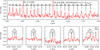 |
Fig. 5 As Fig. 3, but for the CO and OH emission spectra in the S1 knot. |
| In the text | |
|
Fig. 6 Combined best-fit LTE model for 12CO2, 13CO2, C2H2, 13CCH2, HCN, and OH emission in source A+B (red shaded region) overlaid on the continuum subtracted data with an arbitrary flux offset (black). Prominent emission lines are labelled. Best-fit results for individual molecules are shown as the coloured lines below, with the horizontal bars indicating the regions of spectrum used for fitting. Extinction by CO2 ice has been included in the models, which suppresses the flux from the CO2 gas P-branch (see Sect. 2.4). |
| In the text | |
|
Fig. 7 Rotational diagrams of CO υ = 1 − 0 P-branch transitions produced using our LTE slab model for four different column densities at a temperature of T = 1000 K; the colour of each symbol indicates the line optical depth. The dotted line at Eup = 4600 K is the energy above which transitions fall shortwards of the MIRI/MRS blue wavelength limit of 4.9 µm. For each model, the rotational temperature derived from a linear fit to transitions in the MIRI range (i.e. above Eup = 4600 K) is shown by the black lines. |
| In the text | |
|
Fig. 8 Schematic of our proposed origins for the molecular emission and absorption observed towards source A (right half), B (left half), and S1 (outflow shocks, centre) in IRAS 23385+6053. |
| In the text | |
|
Fig. A.1 Example of local continuum spline fitting and modelling of the CO2 (top panel), H2O (middle panel), and |
| In the text | |
|
Fig. A.2 Correction for differential extinction by CO2 ice of the CO2 gas emission features. The blue line shows the continuum subtracted data with the CO2 ice feature removed. The best-fit LTE model of CO2 with extinction correction, but without any correction for ice absorption (orange) overproduces the Q and P-branch emission. The estimated optical depth of the CO2 ice feature (dashed grey line) is applied as a scaling factor to the same best-fit model (green curve), which significantly improves the fit to the Q-branch, though the P-branch features are now somewhat under-produced. |
| In the text | |
|
Fig. B.1 As Figure 6, but for the best-fit LTE models of CO, H2O emission at 5.5–7.7 µm and 16–18 µm in source A. |
| In the text | |
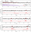 |
Fig. B.2 As Figure 6, but for the best-fit LTE model of CO and OH emission in source S1. |
| In the text | |
|
Fig. B.3 As Figure 6, but the observed data for source B is shown in units of optical depth with an offset of −0.5 relative to the best-fit LTE model for H2O absorption. |
| In the text | |
|
Fig. C.1 Normalized χ2 maps (colour scale) of the LTE model temperature and column density grids for CO2, C2H2, HCN, and OH model fits in source A+B. The best-fit emitting radius for each model is overlaid as white contours, while the 1, 2, and 3 σ confidence interval contours are overlaid in black. The best-fit model at the minimum χ2 is shown by a blue cross. |
| In the text | |
|
Fig. C.2 As Figure C.1, but for CO emission in source A and H2O absorption in source B |
| In the text | |
|
Fig. C.3 As Figure C.1, but for CO and OH emission in source S1. |
| In the text | |
Current usage metrics show cumulative count of Article Views (full-text article views including HTML views, PDF and ePub downloads, according to the available data) and Abstracts Views on Vision4Press platform.
Data correspond to usage on the plateform after 2015. The current usage metrics is available 48-96 hours after online publication and is updated daily on week days.
Initial download of the metrics may take a while.