| Issue |
A&A
Volume 623, March 2019
|
|
|---|---|---|
| Article Number | A122 | |
| Number of page(s) | 28 | |
| Section | Extragalactic astronomy | |
| DOI | https://doi.org/10.1051/0004-6361/201834239 | |
| Published online | 19 March 2019 | |
Relations between abundance characteristics and rotation velocity for star-forming MaNGA galaxies
1
Main Astronomical Observatory, National Academy of Sciences of Ukraine, 27 Akademika Zabolotnoho St, 03680 Kiev, Ukraine
e-mail: pilyugin@mao.kiev.ua
2
Astronomisches Rechen-Institut, Zentrum für Astronomie der Universität Heidelberg, Mönchhofstr. 12–14, 69120 Heidelberg, Germany
3
Kazan Federal University, 18 Kremlyovskaya St., 420008 Kazan, Russian Federation
4
Instituto de Astrofísica de Andalucía, CSIC, Apdo 3004, 18080 Granada, Spain
Received:
13
September
2018
Accepted:
30
January
2019
We derive rotation curves, surface brightness profiles, and oxygen abundance distributions for 147 late-type galaxies using the publicly available spectroscopy obtained by the MaNGA survey. Changes of the central oxygen abundance (O/H)0, the abundance at the optical radius (O/H)R25, and the abundance gradient with rotation velocity Vrot were examined for galaxies with rotation velocities from 90 km s−1 to 350 km s−1. We find that each relation shows a break at Vrot∗ ∼ 200 km s−1. The central (O/H)0 abundance increases with rising Vrot and the slope of the (O/H)0–Vrot relation is steeper for galaxies with Vrot ≲ Vrot∗. The mean scatter of the central abundances around this relation is 0.053 dex. The relation between the abundance at the optical radius of a galaxy and its rotation velocity is similar; the mean scatter in abundances around this relation is 0.081 dex. The radial abundance gradient expressed in dex/kpc flattens with the increase of the rotation velocity. The slope of the relation is very low for galaxies with Vrot ≳ Vrot∗. The abundance gradient expressed in dex/R25 is roughly constant for galaxies with Vrot ≲ Vrot∗, flattens towards Vrot∗, and then again is roughly constant for galaxies with Vrot ≳ Vrot∗. The change of the gradient expressed in terms of dex/hd (where hd is the disc scale length), in terms of dex/Re, d (where Re, d is the disc effective radius), and in terms of dex/Re, g (where Re, g is the galaxy effective radius) with rotation velocity is similar to that for gradient in dex/R25. The relations between abundance characteristics and other basic parameters (stellar mass, luminosity, and radius) are also considered.
Key words: galaxies: abundances / galaxies: kinematics and dynamics / galaxies: ISM
© ESO 2019
1. Introduction
The formation and evolution of galaxies in the lambda cold dark matter (ΛCDM) universe is mainly governed by the host dark matter halo. The dark matter halo makes a dominant contribution to the dynamical mass of a galaxy. Hence the rotation velocity of a disc galaxy, which is a tracer of the dynamical mass is the most fundamental parameter of that disc galaxy. The correlations between the rotation velocity and other basic parameters (stellar mass, size, luminosity) and, consequently, the correlations between each pair of the basic parameters are predicted by simulations (e.g. Mo et al. 1998; Mao et al. 1998; Dutton et al. 2011; Dutton 2012). Empirical scaling relations between the rotation velocity and the luminosity or stellar mass, in other words, the luminous or stellar mass Tully–Fisher (TF) relation (Tully & Fisher 1977; Reyes et al. 2011; McGaugh & Schombert 2015; Straatman et al. 2017), between the rotation velocity and the baryonic mass, in other words, the baryonic TF relation (Walker 1999; Zaritsky et al. 2014; Lelli et al. 2016; Bradford et al. 2016; Übler et al. 2017), and between the rotation velocity and the size (Tully & Fisher 1977; Karachentsev et al. 2013; Böhm & Ziegler 2016; Schulz 2017) for disc galaxies at the present epoch and at different redshifts are established in the papers referenced above along with many others. To reduce the scatter in the relation, a second parameter beyond the rotation velocity is sometimes added, that is, a correlation between TF residuals and an additional parameter is sought.
Is the chemical evolution of galaxies also governed mainly by the dynamical mass (or the host dark matter halo)? On the one hand, it is established that the characteristic oxygen abundance of a galaxy correlates with its rotation velocity, stellar mass, luminosity, and size (Lequeux et al. 1979; Zaritsky et al. 1994; Garnett 2002; Grebel et al. 2003; Pilyugin et al. 2004, 2014a; Tremonti et al. 2004; Erb et al. 2006; Cowie & Barger 2008; Maiolino et al. 2008; Guseva et al. 2009; Thuan et al. 2010; Andrews & Martini 2013; Zahid et al. 2013; Maier et al. 2014; Steidel et al. 2014; Izotov et al. 2015; Sánchez et al. 2017; Barrera-Ballesteros et al. 2017, among many others). On the other hand, the relation of the radial oxygen abundance distribution (gradient) with rotation velocity and other basic parameters of a galaxy is still not well explored. The conclusions on the correlation between the metallicity gradient and basic galaxy parameters reached in recent studies are somewhat controversial.
The radial oxygen abundance distributions across the galaxies measured by the Calar Alto Legacy Integral Field Area (CALIFA) survey (Sánchez et al. 2012a; Husemann et al. 2013; García-Benito et al. 2015) were investigated by Sánchez et al. (2012b, 2014) and Sánchez-Menguiano et al. (2016). These authors found that all galaxies that show no clear evidence of an interaction present a common gradient in the oxygen abundance expressed in terms of dex/Re, d, where Re, d is the disc’s effective radius. The slope is independent of morphology, the extistence of a bar, absolute magnitude, or mass. The distribution of slopes is statistically compatible with a random Gaussian distribution around the mean value. This conclusion was confirmed by the results based on the Multi-unit Spectroscopic Explorer (MUSE) integral field spectrograph observations of spiral galaxies (Sánchez-Menguiano et al. 2018).
Ho et al. (2015) determine metallicity gradients in 49 local field star-forming galaxies. They found that when the metallicity gradients are expressed in dex/R25 (R25 is the B-band isophotal radius at a surface brightness of 25 mag arcsec−2) then there is no correlation between the metallicity gradient and the stellar mass and luminosity. When the metallicity gradients are expressed in dex/kpc, then galaxies with lower mass and luminosity have steeper metallicity gradients, on average.
Belfiore et al. (2017) determine the oxygen abundance gradients in a sample of 550 nearby galaxies in the stellar mass range of 109 M⊙–1011.5 M⊙ with spectroscopic data from the Mapping Nearby Galaxies at Apache Point Observatory (SDSS-IV MaNGA) survey (Bundy et al. 2015). They find that the gradient in terms of dex/Re, d steepens with stellar mass until ∼1010.5 M⊙ and remains roughly constant for higher masses. The gradient in terms of dex/Re, g (where Re, g is the galaxy effective radius) steepens with stellar mass until ∼1010.5 M⊙ and then flattens slightly for higher masses. The gradient in the terms of dex/kpc steepens with stellar mass until ∼1010.5 M⊙ and then becomes flatter again. Thus, differing conclusions on the relation between the metallicity gradient and basic parameters are reached in the studies quoted above.
Our current investigation is motivated by the following deliberations. The oxygen abundances in the papers quoted are estimated through 1D calibrations. In a previous published study we have demonstrated that the 1D N2 calibration produces either a reliable or a wrong abundance depending on whether the excitation and the N to O abundance ratio in the target region is close to or differs from those parameters in the calibrating points (Pilyugin et al. 2018; hereafter Paper I). Ho et al. (2015) also note that the radial change of oxygen abundances derived with two different 1D calibrations can differ significantly when the ionization parameters change systematically with radius. We also demonstrated that the 3D R calibration from Pilyugin & Grebel (2016) produces quite reliable abundances in the MaNGA galaxies.
Here we derive rotation curves, photometric profiles, and R-calibration-based abundances for 147 MaNGA galaxies. We used the obtained rotation velocities, abundances, and photometric parameters coupled with published stellar masses to examine the correlations between chemical properties (oxygen abundances at the centres and at optical radii, and radial gradients) with the rotation velocity and other basic parameters (stellar mass, luminosity, radius) of our target galaxies.
The paper is organized in the following way. The data are described in Sect. 2. In Sect. 3 the relations between the characteristics of our galaxies are examined. Section 4 includes the discussion of our results, and Sect. 5 contains a brief summary.
Throughout the paper, we will use the rotation velocity Vrot in the units of km s−1, the photometric (Mph) and spectroscopic (Msp) stellar masses of a galaxy in the units of M⊙, and the luminosity LB in the units of L⊙. A cosmological model with H0 = 73 km s−1 Mpc−1 and Ωm = 0.27 and ΩΛ = 0.73 is adopted.
2. Data
2.1. Preliminary remarks
The spectroscopic data from the SDSS-IV MaNGA survey provide the possibility (i) to measure the observed velocity fields and derive rotation curves for a large sample of galaxies, (ii) to measure surface brightnesses and derive optical radii and luminosities, and (iii) to measure emission line fluxes and derive abundance maps. The publicly available data obtained in the framework of the MaNGA survey are the basis of our current study. We selected our initial sample of star-forming galaxies (600 galaxies) by visual examination of the images of the SDSS-IV MaNGA DR13 galaxies. The spectrum of each spaxel from the MaNGA datacubes was reduced in the manner described in Zinchenko et al. (2016). For each spectrum, the fluxes of the [O II]λ3727+λ3729, Hβ, [O III]λ4959, [O III]λ5007, [N II]λ6548, Hα, [N II]λ6584, [S II]λ6717, [S II]λ6731 lines were measured. The determinations of the photometrical properties of the MaNGA galaxies is described in Paper I. The determinations of the abundances and the rotation curves is described below.
The SDSS data base offers values of the stellar masses of galaxies determined in different ways. We have chosen the photometric Mph and spectroscopic Msp masses of the SDSS and BOSS galaxies (BOSS stands for the Baryon Oscillation Spectroscopic Survey in SDSS-III, see Dawson et al. 2013). The photometric masses, Mph, are the best-fit stellar masses from database table STELLARMASSSTARFORMINGPORT obtained by the Portsmouth method, which fits stellar evolution models to the SDSS photometry (Maraston et al. 2009, 2013). The spectroscopic masses, Msp, are the median (50th percentile of the probability distribution function, PDF) of the logarithmic stellar masses from table STELLARMASSPCAWISCBC03 determined by the Wisconsin method (Chen et al. 2012) with the stellar population synthesis models from Bruzual & Charlot (2003). The NSA (NASA-Sloan Atlas) data base also offers values of photometric stellar masses of the MaNGA galaxies, Mma. The NSA stellar masses are derived using a Chabrier (2003) initial mass function with Bruzual & Charlot (2003) simple stellar population models. Stellar masses Mma are taken from the extended NSA targeting catalogue1.
2.2. Rotation curve and representative value of the rotation velocity
2.2.1. Approach
The measured wavelength of the emission lines provides the velocity of each region (spaxel). The emission line profile is fitted by a Gaussian, and the position of the centre of the Gaussian is adopted as the wavelength of the emission line. We measured the wavelengths of the Hα and Hβ emission lines. We analysed the velocity map obtained from the Hα emission line measurements in our current study because this stronger line can usually be measured with higher precision than the weaker Hβ line. Thus we can expect that the error in the measured wavelength of the Hα emission line e(λ0) is lower than that for the Hβ emission line. Moreover, the error in the measured wavelength of the Hα line results in a lower error of the velocity e(λ0)/λ0 than the error in the measured wavelength of the Hβ line. Therefore, we obtained the position angle of the major axis of the galaxy, the galaxy’s inclination angle, and the rotation velocity from the analysis of the Hα velocity field.
The determination of the rotation velocity from the observed velocity field is performed in the standard way (e.g. Warner et al. 1973; Begeman 1989; de Blok et al. 2008; Oh et al. 2018). The parameters that define the observed velocity field of a galaxy with a symmetrically rotating disc are as follows:
-
The pixel coordinates (x0 and y0) of the rotation centre of the galaxy.
-
The velocity of the centre of the galaxy with respect to the Sun, the so-called systemic velocity Vsys.
-
The circular velocity Vrot at the distance R from the galaxy’s centre.
-
The position angle PA of the major axis.
-
The angle i between the normal to the plane of the galaxy and the line of sight, the inclination angle.
The observed line-of-sight velocities Vlos recorded on a set of pixel coordinates (x, y) are related to the kinematic parameters by:

where
where R
![$$ \begin{aligned} \begin{array}{lll} R = [ \{ - (x-x_0) \sin (\mathrm{PA}) + (y-y_0) \cos (\mathrm{PA}) \}^{2} \\ \qquad + \{((x-x_0) \cos (\mathrm{PA}) + (y-y_0) \sin (\mathrm{PA}))/\cos i\} ^{2} ]^{1/2} \end{array} \end{aligned} $$](/articles/aa/full_html/2019/03/aa34239-18/aa34239-18-eq10.gif)
is the radius of a ring in the plane of the galaxy (Warner et al. 1973; Begeman 1989; de Blok et al. 2008; Oh et al. 2018).
The deprojected galaxy plane is divided into rings with a width of one pixel. The rotation velocity is assumed to be the same for all the points within the ring. The position angle of the major axis and the galaxy inclination angle are assumed to be the same for all the rings, in other words, constant within the disc. The parameters x0, y0, Vsys, PA, i, and the rotation curve Vrot(R) are derived through the best fit to the observed velocity field Vlos(x, y), meaning we require that the deviation σVlos given by
![$$ \begin{aligned} \sigma _{V_{\rm los}} = \sqrt{ \left[\sum \limits _{j=1}^n (V_{\mathrm{los},j}^\mathrm{cal} - V_{\mathrm{los},j}^\mathrm{obs})^{2}\right] /n} \end{aligned} $$](/articles/aa/full_html/2019/03/aa34239-18/aa34239-18-eq11.gif)
is minimized. Here the  is the measured line-of-sight velocity of the jth spaxel and
  is the velocity computed through Eq. (1) for the corresponding pixel coordinates x and y.
We used two different approaches to derive rotation curves for each galaxy. In the first approach, the values of x0, y0, Vsys, PA, i, and the rotation curve Vrot(R) are derived using all the spaxels with measured Vlos. We refer to this method as case A.
In the second approach, we used an iterative procedure to determine the rotation curve. At each step, data points with large deviations from the rotation curve obtained in the previous step are rejected, and new values of the parameters x0, y0, Vsys, PA, i, and of the rotation curve Vrot(R) are derived. In the first step, the values of x0, y0, Vsys, PA, i, and the rotation curve determined via case A are adopted as values of the previous step. The chosen value of d(Vrot)max is the adopted value of the criterion of the reliability of the spaxel rotation velocity and is used to select data points with reliable rotation velocity Vrot, that is, spaxels where the deviation of the rotation velocity from the rotation curve exceeds d(Vrot)max were rejected. A ring with a width of one pixel usually contains several dozens data points; however, the number of data points in the rings near the centre and at the very periphery of the galaxy can be small. If the number of data points in the ring is lower than three then this ring was excluded from consideration. The iteration was stopped when the absolute values of the difference of x0 (and y0) obtained in successive steps is less than 0.1 pixels, the difference of PA (and i) is smaller than 0.1°, and the rotation curves agree within 1 km s−1 (at each radius). The iteration converges after up to 10 steps. We will refer to this approach as the case B.
2.2.2. Estimation of the uncertainty of the rotation curve caused by errors in the velocity measurements
The errors in the measured line-of-sight velocities Vlos of the spaxels can distort the derived rotation curve. We expect that the validity of the obtained rotation curve may depend on the value of the errors in the line-of-sight velocities and galaxy inclination.
The difference between the values of the spaxel velocity obtained from the measured wavelengths of the Hβ and Hα lines Vlos, Hβ–Vlos, Hα can be considered as some kind of estimation of the error in the spaxel velocity measurements in the MaNGA spectra. Figure 1 shows the normalized histogram of the differences Vlos, Hβ–Vlos, Hα between the measured Hβ and Hα velocities in 46 350 regions (spaxels) in the MaNGA galaxies from Paper I. The mean value of the differences is ∼ − 0.8 km s−1. The mean value of the absolute differences is ∼7 km s−1. Thus we assume that the mean value of the errors in the spaxel velocities in the MaNGA galaxies is near 7 km s−1.
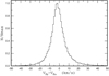 |
Fig. 1. Normalized histogram of the differences VHβ–VHα between the line-of-sight velocities measured for Hβ and Hα emission lines in 46 350 regions (spaxels) in MaNGA galaxies (Pilyugin et al. 2018). |
To examine the influence of the errors in the measured line-of-sight spaxel velocities Vlos on the obtained rotation curve we construct a set of toy models. We fixed the rotation curve and the position angle of the major axis (using PA = 45°). The fields of line-of-sight velocities Vlos were constructed for five values of the inclination angle i = 30°, 40°, 50°, 60°, and 70° using Eqs. (1)–(4). Then we introduced errors in the line-of-sight velocity Vlos of each spaxel. These errors were randomly chosen from a set of errors that follow a Gaussian distribution with σ = 7.
In case A, the rotation curve RCA is determined from each modelled field of line-of-sight velocities using all the data points. In case B, the rotation curve RCB is determined from each modelled set of line-of-sight velocities using the iterative procedure described above. If the deviation of the spaxel rotation velocity from the rotation curve of the previous iteration exceeds a fixed value then this spaxel is rejected. It should be noted that the error in the rotation velocity of the point (spaxel) d(Vrot) depends not only on the error in the line-of-sight velocity d(Vlos) but also on the galaxy inclination i and the position of the region (spaxel) in the galaxy (angle θ). Those errors are related by the expression d(Vrot) = d(Vlos)/(cosθsini) (see Eq. (1)), in other words, the error in the Vrot exceeds the error in the Vlos by a factor of 1/(cosθsini). We adopted the value of the criterion of the reliability of the spaxel rotation velocity d(Vrot)max = 21 km s−1, which exceeds the mean random error in the line-of-sight velocity Vlos measurements by a factor of three.
We have considered 30 models containing six sets of random errors of line-of-sight velocities Vlos for each of the five values of the inclination angle. The models without errors in the line-of-sight velocity Vlos measurements are also considered for comparison.
Panel a1 of Fig. 2 shows the rotation curves for the model of a galaxy with an inclination angle i = 30° obtained for case A. The model rotation curve is shown by the solid line, the rotation curve derived from the modelled map of the line-of-sight velocities without errors by plus signs, and the six rotation curves derived from the modelled map of the line-of-sight velocities with random errors by points. Panel a2 of Fig. 2 shows the same as panel a1 but for the case B of the rotation curve determination. Panels b1 and b2 show the same as panels a1 and a2 but for an inclination angle of i = 50°.
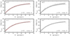 |
Fig. 2. Panel a1: rotation curves for the model of a galaxy with an inclination angle i = 30° obtained for the case A. The solid line is the model rotation curve. The rotation curve derived from the modelled map of the line-of-sight velocities without errors is shown by plus signs. Six rotation curves derived from the modelled maps of the line-of-sight velocities with random errors are indicated by points. Panel a2: same as panel a1 but for the case B. Panels b1 and b2: same as panels a1 and a2 but for an inclination angle of i = 50°. |
The quality of each obtained rotation curve can be specified by the two following characteristics. The first characteristic is the scatter σVrot in the rotation velocities of individual spaxels relative to the obtained rotation curve, which is given by the expression
![$$ \begin{aligned} \sigma _{V_{\rm rot}} = \sqrt{ \left[\sum \limits _{j=1}^n (V_{\mathrm{rot},j}^\mathrm{spaxel} - V_{\mathrm{rot},j}^\mathrm{RC})^{2}\right]/n} \end{aligned} $$](/articles/aa/full_html/2019/03/aa34239-18/aa34239-18-eq14.gif)
where  is the rotation velocity obtained through Eqs. (1)–(4) for the j spaxel of the constructed field of line-of-sight velocities and
  is the rotation velocity given by the inferred rotation curve at the corresponding galacto-centric distance. The second characteristic is the mean shift of the obtained rotation curve in comparison to the true one, that is, the mean value of the deviations d(RC) of the derived rotation curve from the true one (used in the model construction), which is estimated through the expression
![$$ \begin{aligned} d(\mathrm{RC}) = \sqrt{ \left[\sum \limits _{j=1}^n (V_{\mathrm{rot},R_j}^\mathrm{RC} - V_{\mathrm{rot},R_j}^\mathrm{mod})^{2}\right]/n} \end{aligned} $$](/articles/aa/full_html/2019/03/aa34239-18/aa34239-18-eq17.gif)
where  is the obtained rotation velocity at the radius Rj and
  is the rotation velocity given by the true rotation curve at the corresponding galacto-centric distance.
Panel a of Fig. 3 shows the difference between the obtained and true position angle of the major axis as a function of inclination angle for our set of models. Panel b shows the difference between the inferred and true inclination angle as a function of inclination angle. Panel c shows the mean shift of the derived rotation curve relative to the true rotation curve, Eq. (7), as a function of inclination angle. Panel d shows the mean shift of the obtained rotation curve in comparison to the true one as a function of the value of the scatter in the spaxel rotation velocities around the inferred rotation curve, Eq. (6). Cases A and B are shown in each panel by the circles and the plus signs, respectively.
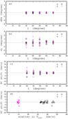 |
Fig. 3. Panel a: difference between the obtained and the true position angle of the major axis d(PA) as a function of inclination angle for our set of models. Panel b: difference between the obtained and the true inclination angle di as a function of inclination angle. Panel c: mean shift of the obtained rotation curve relative to the true rotation curve as a function of the inclination angle. Panel d: mean shift of the obtained rotation curve as a function of the value of the scatter of the spaxel rotation velocities around the obtained rotation curve. Cases A and B are shown by circles and plus signs, respectively, in each panel. |
Examination of Figs. 2 and 3 results in the following conclusions.
-
The rotation curve derived for the case A may involve data points with large deviations.
-
The mean shift of the obtained rotation curve relative to the true one does not exceed ∼5 km s−1 for galaxies with an inclination of i ≳ 40° and can reach up to ∼10 km s−1 for galaxies with i ∼ 30° if the line-of-sight velocity measurements involve random errors with σVlos = 7 km s−1. This is the mean value of the velocity measurement errors estimated from the comparison between the line-of-sight velocities measured for Hβ and Hα emission lines in 46 350 regions (spaxels) in MaNGA galaxies as mentioned earlier.
-
There is no one-to-one correspondence between d(RC) and σVrot, that is, the value of the scatter σVrot in the rotation velocities of individual spaxels around the obtained rotation curve is not a reliable indicator of the deviation d(RC) of the inferred rotation curve from the true one.
Thus, a value of the d(Vrot)max = 21 km s−1 is adopted in the determinations of the rotation curves of the target MaNGA galaxies. One can expect that the deviation d(RC) of the obtained rotation curve from the true rotation curve caused by errors in the velocity measurements does not exceed 10 km s−1 for galaxies with inclination i ≳ 30°.
2.2.3. Rotation curves of target MaNGA galaxies
We derive surface brightness profiles, rotation curves for cases A and B, and abundance distributions for our target MaNGA galaxies. Figure 4 shows the galaxy M-8141-12704, which is one of those galaxies with very good agreement between the rotation curves RCA and RCB. The shift of RCA relative to RCB is only −0.5 km s−1. Figure 5 shows the galaxy M-7975-09101, which is an example of a galaxy with an appreciable difference between RCA and RCB; here the shift between RCA and RCB is −15.6 km s−1. Figures 4 and 5 show the surface brightness distribution across the image of the galaxy in pixel coordinates (panel a1), the derived surface brightness profile (points) and the fit within the isophotal radius with a Sérsic profile for the bulge and a broken exponential for the disc (solid line) (panel a2), the observed velocity Vlos field in pixel coordinates (panel b1), the rotation curve derived for case A (panel b2), the spaxels rejected in the determination of the rotation curve for case B (panel c1), and the rotation curve derived for case B (panel c2). A prominent feature of both Figs. 4 and 5 is that the spaxels rejected in the determination of the rotation curve for the case B are usually located near the minor kinematic axis (the rotation axis) of the galaxies since even a small error in the line-of-sight velocity Vlos measurement results in a large error in the rotation velocity Vrot.
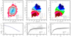 |
Fig. 4. Panel a1: surface brightness distribution across the image of the galaxy M-8141-12704 in sky coordinates (pixels). The value of the surface brightness is colour-coded with a stepsize of d(magB) = 0.5. The plus sign indicates our derived photometric centre of the galaxy. The dashed line is the major photometric axis of the galaxy. The circle denotes the inferred kinematic centre of the galaxy. The solid line indicates the major kinematic axis of the galaxy for the case B. Panel a2: derived surface brightness profile (points, where the surface brightness is given in units of L⊙/pc2 as a function of the fractional optical radius Rg = R/R25) and the fit within the isophotal radius with a Sérsic profile for the bulge and a broken exponential for the disc (line). The surface brightness profile was obtained with kinematic (case B) geometric parameters of the galaxy. Panel b1: observed velocity field in pixel coordinates. The value of the observed velocity is colour-coded with a step size of 30 km s−1. The positions of the photometric centre and the major axis come from panel a1. The cross shows the kinematic centre of the galaxy. The dotted line shows the major kinematic axis of the galaxy for the case A. Panel b2: rotation curve derived for case A. The grey points stand for the obtained rotation velocities of the individual spaxels; the dark points are the mean values of the rotation velocities in rings of a width of 1 pixel. Panel c1: observed velocity field in pixel coordinates as in panel b1 but the spaxels rejected in the determination of the rotation curve for the case B are shown by the green colour. The circle indicates the kinematic centre of the galaxy, and the solid line is the major kinematic axis of the galaxy for case B. The cross is the kinematic centre and the dotted line is the major kinematic axis of the galaxy for the case A. Panel c2: rotation curve derived for case B. The grey points are the measured rotation velocities for individual spaxels; the dark points indicate the mean values of the rotation velocities in rings of a width of one pixel. |
We selected the final sample of the MaNGA galaxies to be analysed by visual inspection of the derived surface brightness profile, rotation curve, and abundance distribution for each galaxy. We used the following criteria.
Spaxels with measured emission lines and surface brightness need to be well distributed across the galactic discs, covering more than ∼0.8R25. Those conditions provide the possibility to estimate reliable intersect values of the rotation velocity, the surface brightness, and the oxygen abundance both at the centre and at the optical radius since the extrapolation is relatively small (if any). It should be noted that only the spaxel spectra where all the used lines are measured with S/N > 3 were considered. Therefore the spaxels with the reliable measured spectra can cover less than ∼0.8R25 even if the spaxel spectra beyond 0.8 R25 are available. 151 galaxies were rejected according to this criterion.
The rotation curve should be more or less smooth. If the obtained rotation velocities show a large irregular variation at some galacto-centric distances then that galaxy was excluded from consideration. The presence of irregular variations in the rotation velocities implies that either the quality of the spectra is not good enough or the rotation is distorted. This prevents an estimation of a reliable rotation curve. The geometric angles were poorly determined in a number of galaxies, that is, the kinematic angles differ significantly from the photometric angles. Barrera-Ballesteros et al. (2014, 2015) have found that disagreement between the kinematic and photometric position angles can be caused by interactions. A galaxy was also excluded from consideration if the values of the inclination angle obtained from the analysis of the velocity field and from the analysis of the photometric map differed by more than 12°. In several cases, one can see clearly that the spiral arms (or bright star formation regions) influence the derived values of the photometric angles. Such galaxies were not rejected even if the disagreement between the kinematic and photometric angles is large. The rotation curves or/and kinematic angles were poorly determined in 157 galaxies. Those galaxies are excluded from further consideration.
Galaxies with an inclination angle less than ∼30° were rejected since even a small error in the inclination angle can result in a large error in the rotation velocity for nearly face-on galaxies. Such small values of the inclination angle were obtained in 84 galaxies.
Galaxies with an inclination angle larger than ∼70° were also rejected (61 galaxies). The fit of the Hα velocity field in galaxies with a large ratio of the major to minor axis can produce unrealistic values of the inclination angle. On the one hand, this may be caused by the problem of the determination of the rotation curves in galaxies with large inclination angles from the Hα velocity field as noted and discussed by Epinat et al. (2008). On the other hand, a seemingly high inclination angle may instead imply that some of those galaxies are not galaxies with thin discs. Since our sample includes low-mass galaxies (the stellar masses of our target galaxies lie in the range from ∼109 M⊙ to ∼1011.5 M⊙) some of them may be irregular galaxies. The intrinsic (three-dimensional) shapes of irregular galaxies have been subject for discussion for a long time (Hubble 1926; Hodge & Hitchcock 1966; van den Bergh 1988; Roychowdhury et al. 2013; Johnson et al. 2017, among others). It is usually assumed that the more massive irregular galalaxies may be considered (at least as the first-order approximation) as a disc. Roychowdhury et al. (2013) find that the intrinsic shapes of irregular galaxies change systematically with luminosity, with fainter galaxies being thicker. The most luminous irregular galaxies have thin discs, and these discs tend to be slightly elliptical (axial ratio ∼0.8).
Our final sample of galaxies selected using the above criteria comprises 147 MaNGA galaxies out of 600 considered galaxies. The selected galaxies are listed in Table A.1.
Panel a of Fig. 6 shows the comparison between the values of the inclination angle obtained from the analysis of the velocity fields, ikin, and from the analysis of the pohometric maps, iphot. The points stand for the individual galaxies. The line indicates equal values. For comparison, the data for the CALIFA galaxies from Holmes et al. (2015) are presented by plus signs. Our ikin–iphot diagram for the MaNGA galaxies is similar to the diagram for the CALIFA galaxies from Holmes et al. (2015). Panel b of Fig. 6 shows the comparison between the kinematic inclination angles derived here and the inclination angles from the HyperLeda2 database (Paturel et al. 2003; Makarov et al. 2014). Panel c shows the comparison between the photometric inclination angles derived here and the inclination angles from the HyperLeda data base. Examination of Fig. 6 shows that the HyperLeda inclination angles are in better agreement with our photometric inclination angles than with the kinematic inclination angles. The credibility of out kinematic inclination angles will be tested below.
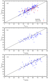 |
Fig. 6. Panel a: comparison between the values of the inclination angle obtained from the analysis of the velocity fields, ikin, and from the analysis of the photometric maps, iphot, for our sample of MaNGA galaxies. The points stand for individual galaxies. The line indicates unity. The plus signs indicate data for CALIFA galaxies from Holmes et al. (2015). Panel b: comparison between the kinematic inclination angles derived here and the inclination angles from the HyperLeda database. Panel c: comparison between the photometric inclination angles derived here and the inclination angles from the HyperLeda database. |
Figure 7 shows the shift of the initial rotation curve (RCA) relative to the final rotation curve (RCB) as a function of rotation velocity Vrot (panel a) and as a function of the scatter in the spaxel velocities around the initial rotation curve (panel b) for our sample of the MaNGA galaxies. Close examination of Fig. 7 shows that the absolute value of the shift RCA–RCB is lower that 5 km s−1 in the majority of our galaxies (112 galaxies out of 147) and exceeds 10 km s−1 only in a few galaxies (12 out of 147).
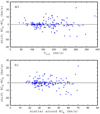 |
Fig. 7. Shift of the initial rotation curve (RCA) relative to the final rotation curve (RCB) as a function of rotation velocity Vrot (panel a) and as a function of the scatter in the spaxel velocities around the initial rotation curve (panel b) for our sample of the MaNGA galaxies. |
2.2.4. Representative value of the rotation velocity
We carried out a least-squares fit of the rotation curve using an empirical “Polyex” curve (Giovanelli & Haynes 2002; Spekkens et al. 2005):

where V0 sets the amplitude of the fit, rpe is a scale length that governs the inner rotation curve slope, and β determines the outer rotation curve slope. The obtained rotation curves for three MaNGA galaxies are shown by grey circles in Fig. 8. The bars denote the mean scatter of the spaxel rotation velocities in rings of one pixel width. The solid line is the fit with the Polyex curve. The asterisk indicates the maximum value of the rotation velocity in the rotation curve fit within the optical radius. Examination of Fig. 8 shows that the Polyex curve is a good approximation for the rotation curves with simple shapes (panels a and b). But the Polyex curve is not a satisfactory approximation for complex rotation curves, for example, rotation curves with a hump (panel c). In this case, the rotation curve fit results in a wrong maximum value of the rotation velocity within the optical radius. To obtain a correct maximum value of the rotation velocity within the optical radius in such cases, we did not fit the whole rotation curve with a Polyex curve but only the outer part of the rotation curve. The points of the rotation curve used in the construction of this fit are marked with crosses in panel c of Fig. 8. The obtained fit is presented by the dashed line, and the maximum value of the rotation velocity within the optical radius is shown by the square.
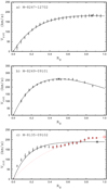 |
Fig. 8. Obtained rotation curve and fit with a Polyex curve for three MaNGA galaxies. Rg is the fractional radius (normalized to the optical radius R25). In each panel, the obtained rotation curve is represented by grey circles. The bars indicate the mean scatter of the spaxel rotation velocities in rings of 1 pixel width. The solid line is the fit with a Polyex curve. The asterisk is the maximum value of the rotation velocity in the rotation curve fit within the optical radius. In panel c, the Polyex curve fit to the outer part of the rotation curve (points marked with red crosses) is presented by a dashed line and the corresponding maximum value of the rotation velocity is indicated by a square. |
The selection of the representative value of the rotation velocity on the rotation curve for the baryonic Tully–Fisher relation is discussed by Stark et al. (2009) and Lelli et al. (2016). They argued that the rotation velocity along the flat part of the rotation curve, Vflat, is the preferable representative value.
We obtain the Vflat value using a simple algorithm similar to that of Lelli et al. (2016). Starting from the centre, R = 0, we obtain the value of Vmean for different galacto-centric distances with a step size of 0.01R25

where hd is the disc’s exponential scale length. At each step we check the condition
We adopt Vflat = Vmean when this condition is satisfied. The exponential scale length hd is estimated using a single exponential profile for the surface brightness distribution of the disc. The surface brightnesses at the optical radius, SLB, R25, and at the centre, SLB, 0, are linked by the expression

The value of the central surface brightness of the disc is obtained from bulge-disc decomposition of the surface brightness profile. The surface brightness at the optical radius is the same for all galaxies by definition. Equation (11) is used to estimate the value of hd for each galaxy. The obtained values of hd for the target galaxies are listed in Table A.1. We note that this definition of the disc scale length hd may be debatable since the surface brightness profiles of the discs of many galaxies are broken, see, for example, panel a2 of Fig. 4.
Using the criterium of Eq. (10), we obtained the rotation velocity along the flat part of the rotation curve Vflat for 81 out of 147 MaNGA galaxies of our sample. We used the maximum rotation velocity within the optical radius as the representative value of the rotation velocity. The influence of the choice of the representative value of Vrot on the result is discussed below.
2.3. Stellar masses of our galaxies
The estimation of the mass of a galaxy is also not a trivial task. The SDSS data base offers values of the stellar masses of galaxies determined in different ways, for example, photometric Mph and spectroscopic Msp masses. Kannappan & Gawiser (2007) have demonstrated that different stellar mass estimation methods yield relative mass scales that can disagree by a factor ≳3. The disagreement between the values of the mass of an individual galaxy produced by the different methods can be around an order of magnitude at 109 M⊙. Even in the case of the best studied galaxies (with accurate distances based on the Cepheid period–luminosity relation or on the brightness of the tip of the red giant branch), the values of the stellar mass determined through the different methods can differ by several times (Ponomareva et al. 2018). This can result in an additional scatter around the mass–metallicity and mass–metallicity gradient diagrams and may mask possible correlations if present.
There is a tight correlation between the rotation velocity and the baryonic (star+gas) mass of a galaxy, the baryonic TF relation (Walker 1999; Zaritsky et al. 2014; Lelli et al. 2016, among many others). Lelli et al. (2016) have found that the intrinsic scatter of the baryonic Tully–Fisher relation is ∼0.1 dex for galaxies in the range from 108 M⊙ to ∼1011 M⊙. The residuals around this relation show no trend with galaxy size or surface brightness. Thus, the rotation velocity is a reliable indicator of the baryonic (star+gas) mass of a galaxy. There is also a tight correlation between the stellar mass of a galaxy and its rotation velocity, the stellar mass TF relation, (Tully & Fisher 1977; Reyes et al. 2011; McGaugh & Schombert 2015, among many others) since the gas mass is a monotonic function of the rotation velocity (e.g. McGaugh & Schombert 2015; Zasov & Zaitseva 2017). Thus, the stellar mass of a galaxy can also be estimated from its rotation velocity.
Panel a of Fig. 9 shows the spectroscopic stellar mass as a function of photometric stellar mass for our sample of galaxies. The points represent data for the individual galaxies. The linear least-squares fit to those data

is shown by the solid line in panel a of Fig. 9. The dashed line indicates exact correspondence in the masses. There is a significant difference between the absolute values of the stellar masses Msp and Mph for our sample of MaNGA galaxies, that is, there is a shift between the zero-points of the Msp and Mph mass scales. Maraston et al. (2013) compare their photometric stellar masses with the spectral stellar masses for a large number of the SDSS galaxies. They find a systematic offset of around 0.2 dex, with the spectroscopic masses being larger than their photometric masses. The difference between the values of the photometric and spectrsoscopic masses for individual galaxies can exceed an order of magnitude (see their Fig. A1). They discuss the sources of difference between the spectroscopic and photometric stellar masses. The mean value of the scatter around the Msp–Mph relation is 0.218 dex.
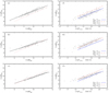 |
Fig. 9. Panel a: spectroscopic stellar mass of our galaxies, Msp, as a function of their photometric stellar mass, Mph. The points represent the individual MaNGA galaxies of our sample. The solid line is the linear best fit to those points. The dotted line indicates exact correpondence in the masses. Panel b: MaNGA stellar mass, Mma, as a function of photometric stellar mass, Mph, and panel c: MaNGA stellar mass, Mma, as a function of spectroscopic stellar mass Msp. The notations are the same as in panel a. Panels d–f: Mph, Msp, and Mma as a function of the rotation velocity Vrot, respectively. The points denote individual galaxies, the solid line is the Mph–Vrot relation (best fit), the long-dashed line is the Msp–Vrot relation, and the short-dashed line is the Mma–Vrot relation. |
Panel b of Fig. 9 shows the MaNGA stellar mass as a function of photometric stellar mass for our sample of galaxies. The points represent the data for the individual galaxies. The linear least-squares fit to those data

is shown by the solid line in panel b of Fig. 9. The dashed line indicates exact correspondence in the masses. The mean value of the scatter around the Mma–Mph relation is 0.186 dex.
Panel c of Fig. 9 shows the MaNGA stellar mass as a function of spectroscopic stellar mass for our sample of galaxies. The points represent data for the individual galaxies. The linear least-squares fit to those data

is shown by the solid line in panel c of Fig. 9. As before, the dashed line indicates exact correspondence in the masses. The mean value of the scatter around the Mma–Msp relation is 0.150 dex.
The mean value of the scatter around the Mx–My relations is between 0.150 dex and 0.218 dex. This value can be interpreted as a mean random error of the relative stellar mass determinations for our MaNGA sample.
Panels d–f of Fig. 9 show the photometric Mph, the spectroscopic Msp, and the MaNGA Mma stellar masses as a function of rotation velocity, respectively. The points in each panel denote the data for the individual galaxies. The solid line is the linear Mph–Vrot relation for galaxies with Vrot > 90 km s−1,

the long-dashed line is the linear Msp–Vrot relation for those galaxies,

the short-dashed line is the linear Mma–Vrot relation for those galaxies,

The mean value of the scatter around the Mph–Vrot relation is 0.283 dex, the mean value of the scatter around the Msp–Vrot relation is 0.233 dex, and the mean value of the scatter around the Mma–Vrot relation is 0.195 dex, that is, the values of the scatter around these M–Vrot relations are close to the values of the scatter around the MX–MY relations. This suggests that the random errors of the relative stellar mass determinations contribute significantly to the scatter around the M–Vrot relations for our MaNGA galaxy sample.
The stellar mass Tully–Fisher relation has been investigated in many works. The comparison of the Mph–Vrot diagram obtained here with the two stellar mass TF relations from Reyes et al. (2011) (for two kinds of stellar mass estimates) and with the relation from McGaugh & Schombert (2015) are shown in panel a of Fig. 10. To make a comparison clear, each relation is shifted along the M-axis in such way that the logM = 10.7 at logVrot = 2.3. Panels b and c show the same as panel a but for the Msp–Vrot and Mma–Vrot relations, respectively. The shifts along the M-axis are 0.029 dex and 0.060 dex for the TF relations A and B from Reyes et al. (2011), –0.029 dex for the relation from McGaugh & Schombert (2015), 0.657 dex for the Mph–Vrot relation, 0.090 dex for the Msp–Vrot relation, and 0.482 dex for the Mma–Vrot relation. The values of the Msp are in much better agreement with the stellar mass TF relations from Reyes et al. (2011) and McGaugh & Schombert (2015) than the Mph and Mma values. The slopes of the Mph–Vrot and Msp–Vrot relations are close to each other. The slope of the Mma–Vrot relation is slightly lower, that is, the Mma masses of the low-mass galaxies may be slightly overestimated or/and the Mma masses of the massive galaxies may be slightly underestimated (see also Fig. 5 in Barrera-Ballesteros et al. 2018).
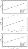 |
Fig. 10. Panel a: comparison of our Mph–Vrot relation with the stellar mass Tully–Fisher relation from McGaugh & Schombert (2015) and two relations (for two kinds of stellar mass estimates) from Reyes et al. (2011). The meaning of each line is described in the legend. Each relation is shifted along the M-axis in such a way that the log M = 10.7 at log Vrot = 2.3. Panels b and c: same as panel a but for the Msp–Vrot and Mma–Vrot relations, respectively. |
Thus, the Msp–Vrot diagram is in much better agreement with the stellar mass TF relations from Reyes et al. (2011) and McGaugh & Schombert (2015) than the Mph–Vrot and the Mma–Vrot diagram. Therefore, the spectroscopic stellar masses Msp will be used below.
The point spread function (PSF) of the MaNGA measurements is estimated to have a full width at half maximum of 2.5 arcsec or five pixels (Bundy et al. 2015; Belfiore et al. 2017). Figure 11 shows the normalized histograms of the galaxy effective radii, the optical radii, and the radii up to which the measurements are available for our sample of galaxies expressed in the units of the PSF (full width at the half maximum). The value of the effective radius of the galaxy is estimated using the photometric profile obtained during the bulge-disc decomposition.
 |
Fig. 11. Normalized histogram of the ratios of the galactic effective radius Re, g to the point spread function PSF (full width at the half maximum) for our sample of galaxies (long-dashed line). The short-dashed line indicates the normalized histograms of the optical radius R25 to the PSF ratios. The solid line denotes the histogram of the radii (expressed in units of PSF) up to which the measurements are available. |
One can expect that the spatial resolution may affect the determined rotation curve especially in the inner part of a galaxy where the change of the rotation velocity with radius is large. Here we consider the maximum rotation velocity value, which is reached in the outer part of a galaxy. Since the rotation curve in the outer part of a galaxy is rather flat then we can expect that the influence of the spatial resolution on the obtained value of the maximum rotation velocity is small, if any. Depending on their angular size, the number of fibres covering the galaxies varied during the observations with the integral field units employed by MaNGA. The panel a of Fig. 12 shows the stellar mass Tully–Fisher relation for our sample of MaNGA galaxies. The galaxies measured with the different numbers of fibres are indicated by different symbols. Inspection of the panel a of Fig. 12 shows that there is no systematic shift in the positions of the galaxies measured with the different numbers of fibres in the stellar Tully–Fisher diagram. The panel b of Fig. 12 shows the comparison of the locations of galaxies with different ratios of galactic effective radius to the point spread function, Re, g/PSF, in the stellar mass–rotation velocity diagram. Galaxies with different Re, g/PSF are indicated by different symbols. Examination of the panel b of Fig. 12 shows that the locations of the galaxies with the different Re, g/PSF ratios follow the same trend. Those two diagrams provide a strong evidence that if there is any influence of the spatial resolution on the obtained value of the maximum rotation velocity in our sample of galaxies, it is small.
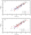 |
Fig. 12. Panel a: stellar mass Tully–Fisher relation for our sample of MaNGA galaxies. Galaxies measured with different numbers of fibres are indicated by different symbols. Panel b: same as panel a but the galaxies with different Re, g/PSF (the ratio of the effective radius of the galaxy to the full width at half maximum of the point spread function) are indicated by different symbols. |
The stellar mass TF relation can be used to test the credibility of the kinematic inclination angles determined here. If the difference between ikin and iphot is caused by the error in the determination of the ikin value then the positions of galaxies with positive values of di = ikin − iphot should show a systematic shift relative to the positions of galaxies with negative values of di. The MaNGA galaxies of our sample with different values of di are shown by different symbols in Fig. 13. There is no systematic shift of the positions of galaxies with different values of di. This suggests that the kinematic inclination angles derived here are quite reliable and the difference between ikin and iphot is not caused by the error in the determination of the ikin value.
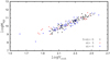 |
Fig. 13. Spectroscopic stellar mass of our galaxies, Msp, as a function of rotation velocity, Vrot. The individual MaNGA galaxies of our sample with different values of di = ikin − iphot are shown by different symbols. |
The stellar mass TF relation can also be used to test the reliability of the choice of the representative value of the rotation velocity. In Fig. 14, we plot Msp as a function of rotation velocity along the flat part of the rotation curve, Vrot, flat, for the galaxies where the Vrot, flat value was obtained (circles). In Fig. 14, we show Msp as a function of maximum rotation velocity within the optical radius Vrot, max for the other galaxies (plus signs). Inspection of Fig. 14 demonstrates that the Msp–Vrot, flat and the Msp–Vrot, flat diagrams are in satisfactory agreement, in other words, the use of the Vrot, max instead of the Vrot, flat does not change the general picture. This suggests that the use of the maximum rotation velocity within the optical radius Vrot, max as the representative value of the rotation velocity is justified.
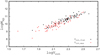 |
Fig. 14. Spectroscopic stellar mass of our galaxies, Msp, as a function of rotation velocity, Vrot. The rotation velocity along the flat part of the rotation curve, Vflat, is shown for the galaxy if this value was obtained (circles). For the other galaxies, the maximum value of the rotation velocity within optical radius is plotted (plus signs). |
3. Abundance and abundance gradient as a function of rotation velocity and other macroscopic characteristics of a galaxy
3.1. Abundance and abundance gradient
We find in a previous study (Pilyugin et al. 2018) that the three-dimensional R calibration, which uses the N2, R2, and R3 lines, produces reliable abundances for regions (spaxels) with H II region-like spectra in the MaNGA galaxies. One should clearly distinguish two questions: the nature of the line-emitting gas (the sources of the ionizing radiation) and the diagnostic of the emitting gas (the abundance determination). The abundance determination through the strong line methods (e.g. our and other calibrations) for objects with H II region-like spectra is based on the fundamental assumption that if two objects have similar spectra (similar relative intensities of the emission lines, normalized to the Hβ line) then the physical conditions and abundances are similar in those objects. This suggests that the calibrations are applicable to any object with an H II region-like spectrum independent of the sources of the ionizing radiation.
The demarcation line between AGNs and H II regions from Kauffmann et al. (2003) in the standard diagnostic diagram of the [N II]λ6584/Hα vs. the [O III]λ5007/Hβ line ratios suggested by Baldwin et al. (1981) is a useful criterion to reject spectra with significantly distorted strengths of the N2 and R3 lines. To examine the distortion of the R2 line, we have compared the behaviour of the line intensities and the abundances estimated through the R calibration for samples of slit spectra of H II regions in nearby galaxies, of the fibre spectra from the SDSS, and of the spaxel spectra of the MaNGA survey for objects located left (or below) of the Kauffmann et al.’s demarcation line in the BPT diagram (Paper I). It has been found that the mean distortion of the R2 (and N2) is less than a factor of ∼1.3. This suggests that the Kauffmann et al.’s demarcation line in the BPT diagram is also a relatively reliable criterium to reject the spectra with distorted strength of the R2 line. Thus, the Kauffmann et al.’s demarcation line in the BPT diagram serves to select objects with H II region-like spectra, that is, to reject the spectra with distorted strengths of the R3, N2, and R2 lines used in determination of the oxygen abundance through the R calibration. It should be noted that the Kauffmann et al.’s demarcation line can be insufficient to distinguish the nature of the line-emitting gas although the regions where photoionization is dominated by hot, low-mass, evolved stars (hDIG regions) are located to the right (or above) of Kauffmann et al.’s demarcation line in the BPT diagram (Lacerda et al. 2018). Here we use Kauffmann et al.’s demarcation line to select spaxels with H II-region-like spectra. All those spaxels are used for the investigation of the abundance distribution across a galaxy. The oxygen abundances for individual spaxels are estimated through the 3D R calibration from Pilyugin & Grebel (2016). It should be noted that the calibrating data points for our 3D R calibration were also selected using the Kauffmann et al.’s demarcation line, in other words, both the calibrating objects and the objects to which the calibration is applied are selected using the same criterion. For comparison, the oxygen abundances are also determined through the widely used N2 and O3N2 indexes introduced by Pettini & Pagel (2004). The N2 and O3N2 calibration relations suggested by Marino et al. (2013) are used.
The radial oxygen abundance distribution in a spiral galaxy is traditionally described by a straight line of the form

where (O/H)* ≡ 12 + log(O/H)(R) is the oxygen abundance at the fractional radius Rg (normalized to the optical radius R25), (O/H) + log(O/H)0 is the intersect central oxygen abundance, and grad is the oxygen abundance gradient expressed in terms of dex/R25. The radial abundance gradients within the optical radius in the discs of the majority of spiral galaxies are reasonably well fitted by this relation although in some cases breaks in the radial abundance gradients near the centre or near the optical radius can occur (e.g. Vila-Costas & Edmunds 1992; Edmunds & Pagel 1984; Zaritsky et al. 1994; van Zee et al. 1998; Pilyugin 2001, 2003; Sánchez et al. 2012b, 2014; Ho et al. 2015; Pilyugin et al. 2014b, 2017a; Zinchenko et al. 2016; Sánchez-Menguiano et al. 2016, 2018). To examine the influence of a possible break in the radial abundance gradient on the central (intersect) abundance and on the abundance at the optical radius (intersect), we also obtained the value of the gradient based on the points with galacto-centric distances within 0.8 > Rg > 0.2 for each galaxy. Figure 15 shows the comparison between the central abundances (and the abundances at the optical radius) obtained from the gradient for the points with galacto-centric distances within 0 < Rg < 1 (labelled case A in Fig. 15) and the central abundances (and the abundances at the optical radius) obtained from the gradient for the points with galacto-centric distances within 0.2 < Rg < 0.8 (labelled case B in Fig. 15). The circles show the central intersect oxygen abundances, and the plus symbols show the intersect oxygen abundance at the optical radius R25. The solid line indicates equal values: the dashed lines show the ±0.05 dex deviation from unity. Inspection of Fig. 15 shows that the central intersect abundances (and the intersect abundances at the optical radius) for cases A and B are in agreement, the mean difference is ∼0.013 dex. This is not surprising, since it is found that the maximum absolute difference between the abundances in a disc given by broken and pure linear relations is less than 0.05 dex for the majority of galaxies (Pilyugin et al. 2017a). The values of the central intersect abundance, the abundance at the optical radius and the radial abundance gradient obtained using the points with galacto-centric distances within 0 < Rg < 1 is examined below.
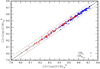 |
Fig. 15. Central intersect oxygen abundance 12 + log(O/H)B for the radial gradient based on the points within 0.2 < Rg < 0.8 as a function of central intersect oxygen abundance 12 + log(O/H)A for the radial gradient based on the points within Rg < 1 (circles). The plus symbols show the same for the intersect oxygen abundance at the optical radius R25. The solid line indicates equal values: the dashed lines show the ±0.05 dex deviation from unity. The oxygen abundances are determined through the R calibration. |
Panel a in Fig. 16 shows the comparison between the abundances obtained through the R calibration of Pilyugin & Grebel (2016) and through the N2 calibration of Marino et al. (2013). The circles are the central intersect oxygen abundances and the plus symbols are the intersect oxygen abundances at the optical radius R25. Panel b in Fig. 16 shows the comparison between the abundances obtained through the R calibration and through the O3N2 calibration. Again the circles are the central intersect oxygen abundances and the plus symbols are the intersect oxygen abundances at the optical radius R25. Panel c in Fig. 16 shows the comparison between the abundance gradients for the R-based, the N2-based and the O3N2-based abundances. The circles show the N2-based gradients vs. the R-based gradients. The plus signs denote the O3N2-based gradients vs. the R-based gradients. Inspection of Fig. 16 shows that the N2-based (and O3N2-based) abundances differ from the R-based abundances, and the difference changes with metallicity.
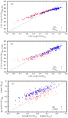 |
Fig. 16. Panel a: comparison between central intersect oxygen abundances based on the abundances obtained through the R calibration of Pilyugin & Grebel (2016) and that based on the abundances obtained through the N2 calibration of Marino et al. (2013) (circles). The plus symbols show the comparison between intersect oxygen abundances at the optical radius R25. Circles in panel b: comparison between central intersect oxygen abundances based on the abundances obtained through the R calibration and that based on the abundances obtained through the O3N2 calibration of Marino et al. (2013). The plus symbols show the comparison between intersect oxygen abundances at the optical radius R25. Circles in panel c: abundance gradient for the N2-based abundances as a function of the abundance gradient for R-based abundances. The plus symbols show the abundance gradient for the O3N2-based abundances as a function of abundance gradient for R-based abundances. The dashed line in each panel indicates equal values. |
Figure 17 demonstrates clearly the origin of the difference between the N2-based (and O3N2-based) and the R-based abundances and the change of the difference with metallicity. The positions of the spectra of the calibrating objects of different metallicities from Pilyugin & Grebel (2016) in the nitrogen line N2 intensity vs. excitation parameter P diagram are shown by the circles in panel a of Fig. 17. The plus symbols show the positions of the MaNGA spaxel spectra with the nitrogen line N2 intensity within −0.600 > log N2 > −0.610. The crosses show the positions of the MaNGA spaxel spectra with 0.265 > log N2 > 0.255. The 1D N2 calibration is based on the assumption that there is a one-to-one correspondence between the oxygen abundance and the nitrogen line N2 intensity, that is, (O/H)N2 = f(N2). In that case all the objects with the same nitrogen line N2 intensity have the same (O/H)N2 abundance. In particular, all the spaxels shown by the plus symbols in the panel a in Fig. 17 have an abundance of 12 + log(O/H)N2 ∼8.2, and all the spaxels shown by the crosses in the panel a in Fig. 17 have 12 + log(O/H)N2 ∼8.6. It is evident from the general consideration, that the nitrogen line N2 intensity in the spectrum of the object depends not only on its oxygen abundance but also on the nitrogen-to-oxygen ratio (N/O) and on the excitation P, i.e. (O/H) = f(N2,N/O,P). The positions of the calibrating objects in the nitrogen line N2 intensity vs. excitation parameter P diagram show clearly that the objects of different metallicities can show a similar nitrogen line N2 intensity depending on its excitation. Then the N2 calibration produces a realistic oxygen abundance in the objects with a given nitrogen line N2 intensity for one value of the excitation parameter P* only. The N2 calibration results in overestimated oxygen abundances for objects with an excitation parameter lower than P* and results in underestimated oxygen abundances for objects with an excitation parameter higher than P*.
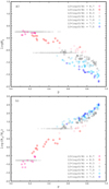 |
Fig. 17. Panel a: nitrogen line N2 intensity vs. excitation parameter P. The circles show the positions of the spectra of the calibrating objects of different metallicities (colour-coded) from Pilyugin & Grebel (2016). The plus symbols show the positions of the MaNGA spaxel spectra with −0.600 > log N2 > −0.610 (which correspond to an N2-based abundance of 12 + log(O/H) ∼8.2). The crosses show the positions of the MaNGA spaxel spectra with 0.265 > log N2 > 0.255 (which correspond to an N2-based abundance of 12 + log(O/H) ∼8.6). Panel b: R3/N2 line ratio vs. excitation parameter P. The plus symbols show the positions of the MaNGA spaxel spectra with 1.105 > log(R3/N2) > 1.095 (which correspond to an O3N2-based abundance of 12 + log(O/H) ∼8.2). The crosses show the positions of the MaNGA spaxel spectra with −0.765 > log(R3/N2) > −0.775 (which correspond to an O3N2-based abundance of 12 + log(O/H) ∼8.6). The notations of the calibrating objects are the same as in panel a. |
It is difficult to indicate the exact value of the P* for a given value of the nitrogen line N2 intensity. The N2 calibration relation from Marino et al. (2013) is based on H II regions with abundances derived through the direct method. Then, the value of P* lies within the interval of excitation parameters covered by the calibrating data points. Inspection of panel a in Fig. 17 shows that the positions of the MaNGA spaxel spectra with −0.600 > log N2 > −0.610 extend significantly towards the lower excitation parameters as compared to the calibrating points. The oxygen abundances in those MaNGA spaxels produced by the N2 calibration are overestimated. On the contrary, the positions of the MaNGA spaxels spectra with 0.265 > log N2 > 0.255 expand towards the higher excitation parameter as compared to the calibrating points. The oxygen abundances in those MaNGA spaxels produced by the N2 calibration are underestimated. Thus, one can expect that the N2-based oxygen abundances should be overestimated, on average, at low metallicities and should be underestimated, on average, at high metallicities. Figure 16 shows just such a behaviour of the N2-based abundances in comparison to the R-based abundances. It should be emphasized that the variation in the N/O ratios is also neglected in 1D calibrations. This results in an additional uncertanty in the oxygen abundances determined through the 1D calibrations.
Panel b of Fig. 17 shows the R3/N2 line ratio vs. excitation parameter P. The plus symbols show the positions of the MaNGA spaxel spectra with 1.105 > log(R3/N2) > 1.095 (which correspond to O3N2-based abundance of 12 + log(O/H) ∼ 8.2). The crosses show the positions of the MaNGA spaxel spectra with −0.765 > log(R3/N2) > −0.775 (which correspond to O3N2-based abundance of 12 + log(O/H) ∼ 8.6). The circles show the positions of the spectra of the calibrating objects of different metallicities (colour-coded) from Pilyugin & Grebel (2016). Examination of panel b in Fig. 17 suggests that the O3N2 calibration results in overestimated oxygen abundances for objects with an excitation parameter lower than P* and results in underestimated oxygen abundances for objects with an excitation parameter higher than P*.
Since the value of the over(under)estimation of the oxygen abundance obtained through the 1D (N2- and O3N2) calibration depends on the metallicity the radial abundance gradient derived using a 1D calibration is not beyond question. The overestimation of the oxygen abundance increases with galacto-centric distance (with the decrease of metallicity) and, as a consequence, the use of the 1D calibration for the abundance determination results in an underestimation of the absolute value of the gradient. Panel c of Fig. 16 shows clearly that the absolute values of the gradients based on the (O/H)N2 abundances are smaller than those for the gradients based on the (O/H)R abundances. The absolute values of the gradients based on the (O/H)O3N2 abundances are also smaller, on average, than those for the gradients based on the (O/H)R abundances.
The change of the over(under)estimation of the oxygen abundance determined through the 1D calibration with galacto-centric distance (with metallicity) can also result in an artificial break in the abundance gradient. Thus, the (O/H)N2 and the (O/H)O3N3 abundances are excuded from consideration. The abundance gradients determined for the (O/H)R abundances in the points with galacto-centric distances within 0 < Rg < 1 and corresponding central abundances and abundances at the optical radius R25 are used in analysis below.
3.2. Properties of the final sample of the galaxies
The maximum rotation velocity within the optical radius is adopted as the representative value of the rotation velocity of a galaxy, Vrot. We used the rotation curve and the values of the position angle of the major axis of the galaxy, PA, and the inclination angle, i, derived for the case B. The surface brightness profile (and, consequently, isophotal radius R25 and disc scale length hd) for each target galaxy and the galacto-centric distances of the spaxels used in the determination of the radial abundance gradient are also estimated with these values of the position angle of the major axis and the inclination angle. The oxygen abundances for individual spaxels are estimated through the 3D R calibration from Pilyugin & Grebel (2016). We adopted the spectroscopic stellar masses Msp of the galaxies. These properties are listed in Table A.1.
Figure 18 shows the properties of our final sample of galaxies, that is, the normalized histograms of the distances to our galaxies in Mpc (panel a), rotation velocities Vrot in km s−1 (panel b), spectroscopic stellar masses Msp in solar units (panel c), luminosities LB in solar units (panel d), optical radii R25 in kpc (panel e), inclination angles i in degrees (panel f), central (intersect) oxygen abundances 12 + log(O/H)0 (solid line) and oxygen abundances at the optical radii 12 + log(O/H)R25 (dashed line) (panel g), and number of points in the velocity map (solid line) and number of points used in the determination of final rotation curve (dashed line) (panel h). The distances were taken from the NASA Extragalactic Database (NED)3. The NED distances use flow corrections for Virgo, the Great Attractor, and Shapley Supercluster infall. The spectroscopic stellar masses are taken from the SDSS data base, table STELLARMASSPCAWISCBC03. Other parameters were derived in our current study. Inspection of Fig. 18 shows that the selected galaxies are located at distances from ∼50 to ∼400 Mpc and show a large variety of physical characteristics. The optical radii of the galaxies cover the interval from around 5 kpc to around 35 kpc. The velocity maps typically contain hundreds or a few thousand data points.
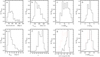 |
Fig. 18. Properties of our sample of galaxies. The panels show the normalized histograms of the distances to our galaxies in Mpc (panel a), rotation velocities Vrot in km s−1 (panel b), spectroscopic stellar masses Msp in solar units (panel c), luminosities LB in solar units (panel d), optical radii R25 in kpc (panel e), inclination angles i in degrees (panel f), central (intersect) oxygen abundances 12 + log(O/H)0 (solid line) and oxygen abundances at the optical radii 12 + log(O/H)R25 (dashed line) (panel g), number of points in the velocity map (solid line), and number of points used in the determination of the final rotation curve (dashed line) (panel h). |
3.3. Relations between oxygen abundance and other macroscopic parameters
Figure 19 shows the central oxygen abundance (O/H)0 (panel a) and the oxygen abundance at the optical radius (O/H)R25 (panel b) as a function of the rotation velocity Vrot. The points represent the individual galaxies; the solid line is the broken (O/H)0–Vrot relation (best fit),

for 90 < Vrot < 200 km s−1, and

for Vrot > 200 km s−1. The dashed line is the broken (O/H)R25–Vrot relation (best fit),

for 90 < Vrot < 200 km s−1, and

for Vrot > 200 km s−1. The notation (O/H)* = 12 + log(O/H) is used for the sake of brevity.
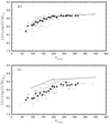 |
Fig. 19. Central oxygen abundance (O/H)0 (panel a) and the oxygen abundance at the optical radius (O/H)R25 (panel b) as a function of the rotation velocity Vrot. The grey points stand for the individual galaxies; the dark points are the binned mean values. The solid line is the broken (O/H)0–Vrot relation, and the dashed line is the broken (O/H)R25–Vrot relation. |
Figure 19 shows that both the central oxygen abundance (O/H)0 and the oxygen abundance at the optical radius (O/H)R25 correlate with the rotation velocity Vrot in a similar way, in the sense that the abundance rises with increasing Vrot and there is a break in the abundance growth rate at  km s−1, that is, the growth rate is lower for galaxies with high rotation velocities. It is difficult to establish the exact value of the dividing rotation velocity
  because of the scatter in the (O/H)–Vrot diagrams. It should be noted that the number of galaxies with Vrot < 90 km s−1 is small in our sample. Therefore we do not discuss galaxies with low rotation velocities in the current study.
The mean value of the residuals of the (O/H)0–Vrot relation is 0.053 dex, and the mean scatter around the (O/H)R25–Vrot relation is 0.081 dex. Thus the oxygen abundance at any galacto-centic distance can be estimated with a mean error of around 0.08 dex from the rotation velocity through the interpolation between the (O/H)0 and (O/H)R25 values obtained from the relations (O/H)0 = f(Vrot) and (O/H)R25 = f(Vrot), respectively.
The increase of both the central oxygen abundance (O/H)0 and the oxygen abundance at the optical radius (O/H)R25 with increasing rotation velocity Vrot is compatible with the so-called “inside-out” scenario for disc growth, where the formation and evolution are faster in the inner part of the disc compared to the outer disc. Within the simple model for the chemical evolution of galaxies the local oxygen abundance is defined by the gas mass fraction (or astration level) at a given galacto-centric distance. It should be noted that the optical radius moves outward during galaxy evolution because the stellar surface mass density at each galacto-centric distance increases with time due to star formation. Since the total (star + gas) surface mass density of the disc decreases with galacto-centric distance, a fixed value of the stellar surface mass density at a larger galacto-centric distance is reached at a larger astration level and, consequently, at a higher oxygen abundance. Thus, the more evolved (the more massive) galaxies have higher astration levels (and, consequently, higher oxygen abundances) both at the centre and at the optical radius.
The left column panels of Fig. 20 show the basic parameters X of a galaxy (where X stands for Msp in panel a1, LB (panel a2), R25 (panel a3), and Mma in panel a4) as a function of the rotation velocity Vrot. The grey points in each panel represent the data for individual MaNGA galaxies from our sample; the dark points are mean values in bins of Vrot. The middle column panels of Fig. 20 show the central oxygen abundance (O/H)0 as a function of the parameters X. The right column panels of Fig. 20 show the oxygen abundance at the optical radius (O/H)R25 as a function of parameters X. The scatter in the central oxygen abundances and in the abundances at the optical radius relative the mean values in bins are reported in Table 1.
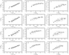 |
Fig. 20. Left column panels: parameters X( = Msp, LB, R25, Mma; from top to bottom) as a function of the value of the rotation velocity Vrot. Middle column panels: central oxygen abundance (O/H)0 as a function of the parameters X. Right column panels: oxygen abundance at the optical radius (O/H)R25 as a function of the parameters X. The grey points on each panel represent the data for individual MaNGA galaxies from our sample; the dark points are the mean values in bins. |
Scatter in the O/H values in the X vs. O/H diagrams.
Inspection of Figs. 19 and 20 show that the variation of both (O/H)0 and (O/H)R25 with any macroscopic parameter X (X = Vrot, Msp or Mma, LB, R25) is similar in the sense that the abundance grows with the increase of the value of the parameters X and there is break in the abundance growth rate at some value of X*, that is, the growth rate becomes lower beyond some value of the parameter X*. Again, it is difficult to establish the exact value of the X* because of the scatter in the (O/H)–X diagrams.
Inspection of the Table 1 shows that the scatter in the central oxygen abundances is minimum in the (O/H)0–Msp diagram being lower than that in the (O/H)0–Vrot diagram. From general considerations, it can be the case that the correlation between the oxygen abundance and the stellar mass tighter than the correlation between the oxygen abundance and the rotation velocity. If the intrinsic scatter in the baryonic Tully–Fisher relation is negligible (McGaugh & Schombert 2015) then the scatter in oxygen abundances in the (O/H)0–Mbaryonic and in the (O/H)0–Vrot diagram for a sample of the purely rotating systems should be similar. The stellar mass of the galaxy is defined by the baryonic mass of the galaxy and the astration level. The oxygen abundance in the galaxy is also defined by the astration level. Therefore the fluctuations in the astration level in the galaxies of a given baryonic mass (a given rotation velocity) result in a larger scatter in the (O/H)0–Vrot than in the (O/H)0–Msp diagram. On the other hand, the scatter in the oxygen abundances is a combination of the intrinsic scatter and that from the random errors in the abundance and stellar mass (rotation velocity) determinations. The difference between the scatter in the (O/H)0–Msp and the (O/H)0–Mma diagrams is larger than the difference between the scatter in the (O/H)0–Msp and the (O/H)0–Vrot diagrams. This may be considered as evidence that the random errors in the abundance and stellar mass (rotation velocity) determinations make a significant contribution to the scatter in those diagrams. Therefore it is difficult to conclude if the intrinsic scatter in the oxygen abundance vs. stellar mass diagram is lower than that in the oxygen abundance vs. rotation velocity diagram.
D’Eugenio et al. (2018) investigate the correlation of the oxygen abundance with the stellar mass Msp and with two parameters that are combinations of the value of the stellar mass and the value of the galactic effective radius (Msp/Re, g and  ) for 68 959 SDSS galaxies. They found that the scatter in the O/H–Msp/Re, g diagram is lower than that in the O/H–Msp and in the O/H–
 diagrams. The oxygen abundances measured in the SDSS galaxies can be considered as central oxygen abundances. The radial abundance gradients determined here provide a possibility to examine the correlation of the oxygen abundance at any fixed galacto-centric distance with the parameters considered by D’Eugenio et al. (2018). We consider the central oxygen abundance (O/H)0, the oxygen abundance at the galactic effective radius (O/H)Re, g, and the abundance at the optical radius (O/H)R25. Figure 21 shows those values of the oxygen abundance as a function of stellar mass Msp and of the parameters Msp/Re, g and
  . The grey points in each panel are the data for individual MaNGA galaxes from our sample, while the dark points are the binned mean values. The scatter in the abundances in those diagrams relative to the mean values in bins is reported in Table 1.
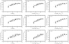 |
Fig. 21. Central oxygen abundance (row a panels), the abundance at the galaxy effective radius (row b panels), and at the optical radius (row c panels) as a function of the stellar mass Msp (left column panels), as a function of Msp/Re, g (middle column panels), and as a function of |

Inspection of Fig. 21 and Table 1 shows that the scatter in the central oxygen abundances (O/H)0 for our sample of MaNGA galaxies is minimum in the (O/H)0–Msp diagram, the scatter in the oxygen abundances at the galaxy effective radius (O/H)Re, g is similar (minimum) in the (O/H)Re, g–Msp and in the (O/H)Re, g–Msp/Re, g diagrams, and the scatter in the oxygen abundances at the optical radius (O/H)R25 is minimum in the (O/H)R25– diagram. Then it is difficult to conclude if our data are in agreement or conflict with the conclusion of D’Eugenio et al. (2018).
Thus, the variation of both (O/H)0 and (O/H)R25 with any macroscopic parameter X (X = Vrot, Msp or Mma, LB, R25) is similar in the sense that the abundance grows with the increase of the value of the parameters X and there is break in the abundance growth rate at some value of X*, in other words, the growth rate becomes lower beyond some value of the parameter X*. It is difficult to establish the exact value of the X* because of the scatter in the (O/H)–X diagrams.
3.4. Oxygen abundance gradient as a function of the macroscopic parameters
As mentioned above, the radial oxygen abundance distribution in a spiral galaxy is traditionally described by a straight line of the form

where (O/H)* ≡ 12 + log(O/H)(R) is the oxygen abundance at the galacto-centric distance R, (O/H) + log(O/H)0 is the extrapolated central oxygen abundance, graddex/Rscale is the slope of the oxygen abundance gradient expressed in terms of dex/Rscale, and Rscale is the adopted radial scale.
Different radial scalings are used to quantify the radial abundance variation in the discs of spiral galaxies. An absolute physical radius in kiloparsecs (Rscale = 1) and different dimensionless radii normalized to the isophotal radius (Rscale = R25) or to the Holmberg radius (Rscale = R26.5) of the galaxy, normalized to the disc exponential scale length (Rscale = hd), normalized to the effective (or half-light) radius of the disc (Rscale = Re, d) or the effective radius of the galaxy (Rscale = Re, g) were used to specify the radial abundance distributions in galaxies (Smith 1975; Alloin et al. 1979; Vila-Costas & Edmunds 1992; Oey & Kennicutt 1993; Zaritsky et al. 1994; Ryder 1995; Garnett et al. 1997; Garnett 1998; Pilyugin et al. 2004, 2015; Sánchez et al. 2012b, 2014; Ho et al. 2015; Bresolin & Kennicutt 2015; Belfiore et al. 2017, among many others). We consider here the values of the gradients for five radial scales (Rscale = 1, hd, R25, Re, d, Re, g), that is, the gradients are expressed in the terms of dex/kpc, dex/hd, dex/R25, dex/Re, d, and dex/Re, g.
The left column panels of Fig. 22 show the oxygen abundance gradients in units of dex/kpc as a function of rotation velocity Vrot (panel a1), spectroscopic stellar mass Msp (panel b1), luminosity in the B-band LB (panel c1), optical radius R25 (panel d1), and stellar mass Mma (panel e1) for our sample of galaxies. The grey points in each panel represent the individual galaxies, and the dark points are the binned mean values. The middle column panels of Fig. 22 show the oxygen abundance gradients in units of dex/R25 as a function of Vrot, Msp, LB, R25, and Mma. The dashed line is the mean value of the gradient –0.200 dex/R25 for our sample of galaxies. The right column panels of Fig. 22 show the oxygen abundance gradients in units of dex/hd as a function of Vrot, Msp, LB, R25, and Mma. The dashed line shows the mean value of the gradient –0.081 dex/hd for our sample of galaxies. The scatter in the gradients relative to the mean values in bins is reported in Table 2.
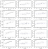 |
Fig. 22. Radial abundance gradient measured in dex/kpc (left column panels), with respect to the optical radius R25 (middle column panels), and with respect to the disc scale length hd (right column panels). Row a panels: radial abundance gradient as a function of the rotation velocity Vrot, row b panels: as a function of the stellar mass Msp, row c panels: as a function of galaxy luminosity LB, row d panels: as a function of optical radius R25, and row e panels: as a function of the stellar mass Mma. The grey points at each panel are the data for individual MaNGA galaxies from our sample, while the dark points are the binned mean values. The dashed line in the middle and right column panels show the mean values of the gradient in units of dex/R25 and dex/hd, respectively. |
Scatter in the radial oxygen abundance gradients in the gradient vs. X diagrams.
The left column panels of Fig. 23 show the radial abundance gradient in units of dex/Re, d as a function of rotation velocity Vrot (panel a1), spectroscopic stellar mass Msp (panel b1), luminosity in the B-band LB (panel c1), optical radius R25 (panel d1), and stellar mass Mma (panel e1) for our sample of galaxies. The grey points in each panel stand for the individual galaxies, and the dark points are the binned mean values. The dashed line is the mean value of the gradient –0.136 dex/Re, d for our sample of galaxies. The value of the disc effective radius Re, d is proportional to the disc scale length, Re, d = 1.67835 hd, (Sánchez et al. 2014). The right column panels of Fig. 23 show the oxygen abundance gradients in units of dex/Re, g as a function of Vrot, Msp, LB, R25, and Mma, respectively. The dashed line is the mean value of the gradient, −0.095 dex/Re, g, for our sample of galaxies. The scatter in the gradients with respect to the mean values in bins is listed in Table 2.
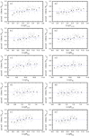 |
Fig. 23. Radial abundance gradient measured in dex/Re, d (left column panels) and dex/Re, g (right column panels). Row a panels: radial abundance gradient as a function of the rotation velocity Vrot, row b panels: as a function of the stellar mass Msp, row c panels: as a function of galaxy luminosity LB, row d panels: as a function of optical radius R25, and row e panels: as a function of the stellar mass Mma. The grey points at each panel are the data for individual MaNGA galaxes from our sample, while the dark points are the binned mean values. The dashed line in the left and right column panels show the mean values of the gradient in units of dex/Re, d and dex/Re, g, respectively. |
Examination of panel a1 of Fig. 22 shows that the oxygen abundance gradients in units of dex/kpc flatten with the increase of the rotation velocity and there is a break in the rate of flattening at Vrot ∼ 200 km s−1 in the sense that the flattening rate with increasing Vrot is lower for galaxies with high rotation velocities. The left column panels of Fig. 22 show that the behaviour of the change of the oxygen abundance gradients in units of dex/kpc is similar for increasing Vrot, Msp, Mma, LB, and R25.
Inspection of panel a2 of Fig. 22 shows that the abundance gradient expressed in dex/R25 is rougly constant for Vrot ≲ 200 km s−1, shows a break at Vrot ∼ 200 km s−1, and remains again roughly constant for higher rotation velocities. The middle column panels of Fig. 22 show that the general picture of the change of the oxygen abundance gradient in units of dex/R25 kpc with any mascroscopic parameter X (X = Msp, Mma, LB, R25) is similar to that for Vrot, in the sense that the mean value of the oxygen abundance gradient for the objects with X < X* differs from that for objects with X > X*, see Table 3.
Mean values of the radial abundance gradient for objects with X < X* and X > X*.
A comparison between the middle and right column panels of Fig. 22 shows that the general picture of the variation of the oxygen abundance gradient in units of dex/R25 kpc and in units of dex/hd is similar. This is because there is no significant change in the ratio of the disc scale length to the optical radius hd/R25 as a function of rotation velocity Vrot for our sample of galaxies; see panel a of Fig. 24. A comparison between Figs. 22 and 23 shows that the qualitative trends in the variation of the oxygen abundance gradient in units of dex/R25 kpc and in units of dex/Re, g is also similar. Again, this is because of the change in the ratio of the galactic effective radius to the optical radius Re, g/R25 as a function of rotation velocity Vrot for our sample of galaxies is rather small as can be seen in panel b of Fig. 24. The variation of the oxygen abundance gradient in units of dex/hd kpc and in units of dex/Re, d is similar because those gradients differ by a constant factor only. It was noted above that the definition of the disc scale length hd may be debatable for many galaxies since the surface brightness profile of the disc is often broken.
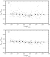 |
Fig. 24. Panel a: ratio of the disc scale length to the optical radius hd/R25 as a function of the value of the rotation velocity Vrot. The grey points represent the data for individual MaNGA galaxies from our sample, and the dark points indicate the binned mean values (omitting objects with hd/R25 > 0.7). The dotted line is the mean hd/R25 value. Panel b: same as panel a but for the ratio of the effective radius of the galaxy to the optical radius Re, g/R25. |
Thus, the radial abundance gradient expressed in dex/kpc flattens with the increase of the rotation velocity. The slope of the relation is very low for galaxies with  . The abundance gradient expressed in dex/R25 is rougly constant for galaxies with
  , flattens towards
  , and then again is roughly constant for galaxies with
  . The change of the gradient expressed in terms of dex/hd, dex/Re, d, and dex/Re, g with rotation velocity is similar to that for the gradient in dex/R25. The qualitative trends in the relations between abundance gradients and other basic parameters (stellar mass, luminosity, and radius) are similar to the trend of the abundance gradient vs. rotation velocity relation.
4. Discussion
In this study, we have considered galaxies with different angular sizes, implying that differing numbers of fibres are needed to cover them when observing them with integral field units (IFUs) as employed by MaNGA. Belfiore et al. (2017) discussed that the abundance distribution obtained in a MaNGA galaxy can depend on the conditions of the observations, that is, on the ratio of the galaxy effective radius Re, g to the PSF or on the number of the fibres with which a galaxy was covered.
Panel a of Fig. 25 shows the (O/H)0–Vrot diagram (the same as panel a of Fig. 19) but marking galaxies observed with different numbers of fibres by different symbols. We see that galaxies observed with differing numbers of fibres still follow the same trend in the (O/H)0–Vrot diagram. Panel b of Fig. 25 shows the (O/H)R25–Vrot diagram (the same as panel b of Fig. 19) but again the galaxies are marked with different symbols according to the number of IFU fibres with which they were observed. Panel b of Fig. 25 demonstrates that the galaxies again follow a single trend in the (O/H)R25–Vrot diagram. The panels c and d of Fig. 25 show the (O/H)R0–Msp and the (O/H)R25–Msp diagrams. The value of the Msp for the galaxy measured with 37 fibres is not available. As before, we can see that the galaxies observed with different numbers of IFU fibres follow a single trend. This suggests that the derived properties of our galaxies do not depend on the number of fibre bundles.
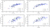 |
Fig. 25. Panel a: central oxygen abundance as a function of rotation velocity for our sample of MaNGA galaxies. Depending on their angular size, the number of fibres covering the galaxies varied during the observations with the integral field units employed by MaNGA. The differing numbers of fibres are indicated by different symbols. Panel b: same as panel a but for the oxygen abundances at the isophotal radius. Panel c: central oxygen abundance as a function of stellar mass Msp. Again the different numbers of fibres are indicated by different symbols. Panel d: same as panel c but for the oxygen abundances at the isophotal radius. The value of the Msp for the galaxy measured with 37 fibres is not available. |
Belfiore et al. (2017) find that the influence of the PSF on the obtained value of the oxygen abundance is maximum at the centre of the galaxy and can be as large as up to around 0.04 dex for a galaxy with Re, g/PSF = 1.5 and inclination angle i = 60°. The mean value of the Re, g/PSF for our sample of galaxies is around 2.75 (Fig. 11). Belfiore et al. (2017) find that the uncertainty in the central oxygen abundance due to the PSF for galaxies with Re, g/PSF = 3.0 is around around 0.02 dex or lower depending on the value of the inclination angle. Thus, the lack of the dependence of the obtained oxygen abundances on the number of the fibre bundles that we noted is in line with the results of Belfiore et al. (2017).
The mass–metallicity (or luminosity–metallicity) relation at the present epoch and its evolution with redshift has been considered previously by numerous authors (Lequeux et al. 1979; Zaritsky et al. 1994; Garnett 2002; Grebel et al. 2003; Tremonti et al. 2004; Erb et al. 2006; Pilyugin et al. 2007, 2013, 2014a; Cowie & Barger 2008; Maiolino et al. 2008; Guseva et al. 2009; Thuan et al. 2010; Pilyugin & Thuan 2011; Rosales-Ortega et al. 2012; Andrews & Martini 2013; Zahid et al. 2013; Maier et al. 2014; Steidel et al. 2014; Izotov et al. 2015; Sánchez et al. 2017; Barrera-Ballesteros et al. 2017, among many others). Different methods to estimate abundances were used in different works, which led to considerable discrepancies in the resulting oxygen abundances due to the differing abundance scales in those papers. Therefore, it is difficult to compare quantitatively the mass (luminosity)–metallicity relations derived by other authors and the ones obtained here.
In Pilyugin et al. (2017b), mass–metallicity relations for a large sample of SDSS galaxies at different redshifts were determined, measuring their oxygen abundances through the same calibration as used here. Figure 26 shows the comparison of the mass–metallicity diagram obtained in our current study for galaxies from the MaNGA survey with the mass–metallicity relation determined for the SDSS galaxies of Pilyugin et al. (2017b). MaNGA galaxies with redshift z < 0.05 are shown by circles, and galaxies with z > 0.05 are indicated by plus signs. The solid line is the O/H–Msp relation obtained for the large sample of SDSS galaxies with z = 0.03 in Pilyugin et al. (2017b). Figure 26 shows that the locations of the MaNGA galaxies in the mass–metallicity diagram agree well with the mass–metallicity relation determined for the other SDSS galaxies. We note that the abundances determined from the SDSS spectra are also in good agreement with abundances determined from the CALIFA spectra (Figs. 16 and 17 in Pilyugin et al. 2017a).
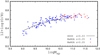 |
Fig. 26. Oxygen abundance as a function of the spectroscopic stellar mass. The oxygen abundances at the centres of individual MaNGA galaxies with redshift z < 0.05 are shown by circles, and those for galaxies at z > 0.05 are shown by plus signs. The solid line is the O/H–Msp relation obtained for a large sample of SDSS galaxies with redshift z = 0.03 in Pilyugin et al. (2017b). |
Panel a of Fig. 27 shows the stellar mass as a function of redshift for our galaxy sample. One can see the sequences of the primary (“low redshift”) and secondary (“high redshift”) sub-samples of the MaNGA targets (Bundy et al. 2015; Wake et al. 2017). Figure 27 shows that the galaxies with masses logMsp ≲ 10 are at redshifts less than ∼0.05 (i.e. spread over the small interval of redshift) and only the most massive galaxies (logMsp ≳ 11) are observed at redshifts up to ∼0.1. Panel b of Fig. 27 shows the stellar mass Tully–Fisher relation for our sample of galaxies. Panels c and d of Fig. 27 show the central oxygen abundance (panel c) and the oxygen abundance at the optical radius (panel d) as a function of stellar mass of the galaxies. In each panel, the galaxies of the primary and secondary sub-samles are denoted by different symbols. Examination of the panels b, c, and d of Fig. 27 shows that the regions of the locations of the galaxies of the primary and secondary sub-samples in different diagram are rather close to each other. A small shift of the locations of the massive galaxies of the secondary sub-sample towards the lower abundances in comparison to the locations of the galaxies of the primary sub-sample in the (O/H)R25–Msp diagram cannot be excluded. Since the shift is small (within around 0.05 dex) and the number of galaxies in this region of the diagram is also small therefore the validity of this shift is not beyond the question. If this shift is real then this can be considered as evidence in favour of the evolutionary changes at the outer parts of the galaxies of the primary (low redshift) sub-sample as compared to the galaxies of the secondary (high redshift) sub-sample. However, larger numbers of massive galaxies of both sub-samples should be considered in order to draw a solid conclusion. The locations of the massive galaxies of the secondary sub-sample and of the primary sub-sample in the (O/H)0–Msp diagram are close to each other. In Pilyugin et al. (2017b) we note that the evolutionary change of the central oxygen abundance in massive galaxies with redshifts from z ∼ 0.025 to ∼0.1 is minor.
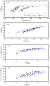 |
Fig. 27. Panel a: stellar mass as a function of redshift for our galaxy sample. The galaxies of the primary (“low redshift”) and secondary (“high redshift”) sub-samples of the MaNGA targets (Bundy et al. 2015; Wake et al. 2017) are shown by different symbols. Panel b: stellar mass Tully–Fisher relation for those galaxies. Panels c and d: central oxygen abundance (panel c) and the oxygen abundance at the optical radius (panel d) as a function of stellar mass of the galaxy. |
Abundance gradients in galactic discs are considered in several recent studies. Again it is difficult to quantitatively compare the results from different works since different methods to estimate abundances were used. Thus we restricted ourselves to the comparison of the general behaviour of the radial abundance gradient with stellar mass obtained here and by other groups of investigators.
We found that the gradient expressed in units of dex/R25 is slightly shallower in massive galaxies although it remains roughly constant both for the subsample of low-mass galaxies and for the subsample of massive galaxies. The behaviour of the gradient expressed in units of dex/hd, dex/Re, d, and dex/Re, g is similar to that for the gradient expressed in dex/R25. The relation between the gradient expressed in units of dex/Re, d and stellar mass was considered recently by Sánchez et al. (2012b, 2014), Sánchez-Menguiano et al. (2016, 2018), and Belfiore et al. (2017). Sánchez et al. (2012b, 2014), and Sánchez-Menguiano et al. (2016) find that all the CALIFA galaxies without clear evidence of an interaction present a common gradient in the oxygen abundance expressed in terms of dex/Re, d. The slope is independent of morphology, the existence of a bar, the absolute magnitude, or the mass. This conclusion is confirmed by the investigation of gradients based on MUSE observations of galaxies (Sánchez-Menguiano et al. 2018). Ho et al. (2015) find that when the metallicity gradients are expressed in dex/R25 then there is no correlation between the metallicity gradient and the stellar mass and luminosity. Belfiore et al. (2017) determine the oxygen abundance gradients in a sample of 550 nearby galaxies from the MaNGA survey. They find that the gradient in terms of dex/Re, d steepens with stellar mass until ∼1010.5 M⊙ and remains roughly constant for higher masses. We note that the lack of a correlation between the abundance gradient expressed in units of dex/hd and the luminosity has already been found in earlier studies (Zaritsky et al. 1994; Garnett et al. 1997).
In our current work, we find that the gradient expressed in dex/kpc flattens with increasing stellar mass. Ho et al. (2015) and Belfiore et al. (2017) also examine the relation between the gradient in units of dex/kpc and stellar mass. Ho et al. (2015) determine metallicity gradients in 49 local field star-forming galaxies. They find that when the metallicity gradients are expressed in dex/kpc then galaxies with lower mass and luminosity have, on average, steeper metallicity gradients. In contrast, Belfiore et al. (2017) find that the gradient in terms of dex/kpc steepens with stellar mass until ∼1010.5 M⊙, while becoming flatter again afterwards. The change of the abundance gradient expressed in units of dex/kpc with stellar mass obtained here agrees with the result of Ho et al. (2015).
Thus, the oxygen abundance of a star-forming galaxy correlates tightly with (and appears to be governed by) its rotational velocity. The central oxygen abundance (O/H)0 and the abundance at the optical radius (O/H)R25 can be found from the rotation velocity with a mean uncertainy of around 0.05 and 0.08 dex, respectively. Consequently, the oxygen abundance at any galacto-centric distance can be found through interpolation between those values with a mean uncertainty of 0.08 dex. The observed scatter in the O/H–Vrot relation is a combination of the intrinsic scatter and errors in the O/H and Vrot measurements, and can be considered as an upper limit on the intrinsic scatter. The abundance deviations of the majority of the target galaxies from the (O/H)0–Vrot and the (O/H)R25–Vrot relations are within ∼0.1 dex (see Fig. 19). The uncertainty in the central oxygen abundance and in the abundance at the optical radius caused by the errors in the oxygen abundance determination in individual regions (spaxels) and by the approximation of the radial abundance distribution by a single straight line can be around ∼0.05 dex (Pilyugin & Grebel 2016; Pilyugin et al. 2017a), meaning that it is comparable to the scatter in the (O/H)0–Vrot and/or (O/H)R25–Vrot diagrams.
It is known that the star formation history of a galaxy is related to its stellar mass, the downsizing effect (Gavazzi 1993; Cowie et al. 1996; Ibarra-Medel et al. 2016). It has also been known for a long time that the morphological Hubble type of a galaxy, expressed in terms of the T-type, is an indicator of its star formation history (e.g. Sandage 1986). The morphological type can contribute to the relations between properties of a galaxy. For example, Muñoz-Mateos et al. (2015) find that the galaxies of different Hubble types populate different areas in the stellar mass–R25.5 diagram, defining clearly distinct sequences. A well defined transition takes place when moving from Sc to Scd galaxies, in the sense that earlier-type galaxies are up to a factor of approximately ten more massive than later-type ones for the same size or isophotal radius R25.5. Therefore, one may expect that the morphological type of a galaxy should be considered as a basic characteristic of a galaxy.
However, Conselice (2003) notes that spiral galaxy classification systems are in many ways not very useful since the most popular morphological classification systems have non-physical and often purely descriptive classification criteria based on optical morphologies that do not uniquely identify, or distinguish, the morphological types of distant galaxies. The estimations of the morphological type of some galaxies from our list can be found in the HyperLeda database (Paturel et al. 2003; Makarov et al. 2014). However, the uncertainty of the numerical T-type can exceed three. Hence we do not consider the morphological types of galaxies here.
5. Summary
The publicly available data obtained within the framework of the MaNGA survey are the base of our current study. We measured the emission lines in the spectrum of each spaxel from the MaNGA datacubes for a sample of late-type galaxies. The wavelengths of the Hα line provide the observed velocity field. We derive rotation curves, surface brightness profiles, and oxygen abundance distributions for 147 galaxies. These data coupled with the available estimations of the stellar masses were used to examine the relations between abundance characteristics (abundances at the centre and at the optical radius, radial gradient) and basic galaxy parameters (rotation velocity, stellar mass, luminosity, radius).
We find that both the central oxygen abundance (O/H)0 and the abundance at the optical radius of a galaxy (O/H)R25 correlate tightly with the rotational velocity. The mean value of the scatter around the (O/H)0–Vrot relation is ∼0.053 dex and the scatter around the (O/H)R25–Vrot relation is ∼0.081 dex. Thus, the oxygen abundances at any galacto-centric distance can be found through interpolation between those values with a mean uncertainty of around 0.08 dex.
The change of both (O/H)0 and (O/H)R25 with Vrot is similar. The abundance grows with increasing Vrot. There is a break in the abundance growth rate at Vrot ∼ 200 km s−1, in the sense that the growth rate is lower for galaxies with high rotation velocities. Both the central oxygen abundance and the abundance at the optical radius of a galaxy correlate with other basic parameters (stellar mass, luminosity, radius) in a similar way as with the rotational velocity.
The oxygen abundance gradients in units of dex/kpc flatten with increasing rotational velocity. Again there is a break in the flattening rate at Vrot ∼ 200 km s−1 in the sense that the flattening rate is lower for galaxies with high rotation velocities. The behaviour of the variation of the oxygen abundance gradients in units of dex/kpc as a function of Vrot, stellar masses Msp and Mma, B-band luminosities LB, and R25 is similar.
The gradient expressed in units of dex/R25 is slightly shallower in galaxies with high rotation velocities although remains roughly constant both for the sub-sample of galaxies with low rotation velocities (Vrot ≲ 200 km s−1) and the sub-sample with high rotation velocities (Vrot ≳ 200 km s−1). The behaviour of the gradient expressed in units of dex/hd, dex/Re, d, and dex/Re, g is similar to that for the gradient expressed in dex/R25.
The NASA/IPAC Extragalactic Database (NED) is operated by the Jet Propulsion Laboratory, California Institute of Technology, under contract with the National Aeronautics and Space Administration. http://ned.ipac.caltech.edu/
Acknowledgments
We are grateful to the referee for his/her constructive comments. L.S.P., E.K.G., and I.A.Z. acknowledge support within the framework of Sonderforschungsbereich (SFB 881) on “The Milky Way System” (especially subproject A05), which is funded by the German Research Foundation (DFG). L.S.P. and I.A.Z. thank for their hospitality of the Astronomisches Rechen-Institut at Heidelberg University, where part of this investigation was carried out. I.A.Z. acknowledges the support of the Volkswagen Foundation under the Trilateral Partnerships grant No. 90411. I.A.Z. acknowledges the support by the Ukrainian National Grid project (especially subproject 400Kt) of the NAS of Ukraine. J.M.V acknowledges financial support from projects AYA2017-79724-C4-4-P, of the Spanish PNAYA, and Junta de Andalucia Excellence PEX2011-FQM705. This work was partly funded by the subsidy allocated to Kazan Federal University for the state assignment in the sphere of scientific activities (L.S.P.). We acknowledge the use of the HyperLeda database (http://leda.univ-lyon1.fr). Funding for SDSS-III has been provided by the Alfred P. Sloan Foundation, the Participating Institutions, the National Science Foundation, and the U.S. Department of Energy Office of Science. The SDSS-III web site is http://www.sdss3.org/. SDSS-III is managed by the Astrophysical Research Consortium for the Participating Institutions of the SDSS-III Collaboration including the University of Arizona, the Brazilian Participation Group, Brookhaven National Laboratory, Carnegie Mellon University, University of Florida, the French Participation Group, the German Participation Group, Harvard University, the Instituto de Astrofisica de Canarias, the Michigan State/Notre Dame/JINA Participation Group, Johns Hopkins University, Lawrence Berkeley National Laboratory, Max Planck Institute for Astrophysics, Max Planck Institute for Extraterrestrial Physics, New Mexico State University, New York University, Ohio State University, Pennsylvania State University, University of Portsmouth, Princeton University, the Spanish Participation Group, University of Tokyo, University of Utah, Vanderbilt University, University of Virginia, University of Washington, and Yale University. Funding for the Sloan Digital Sky Survey IV has been provided by the Alfred P. Sloan Foundation, the U.S. Department of Energy Office of Science, and the Participating Institutions. SDSS-IV acknowledges support and resources from the Center for High-Performance Computing at the University of Utah. The SDSS web site is www.sdss.org. SDSS-IV is managed by the Astrophysical Research Consortium for the Participating Institutions of the SDSS Collaboration including the Brazilian Participation Group, the Carnegie Institution for Science, Carnegie Mellon University, the Chilean Participation Group, the French Participation Group, Harvard-Smithsonian Center for Astrophysics, Instituto de Astrofísica de Canarias, The Johns Hopkins University, Kavli Institute for the Physics and Mathematics of the Universe (IPMU)/University of Tokyo, Lawrence Berkeley National Laboratory, Leibniz Institut für Astrophysik Potsdam (AIP), Max-Planck-Institut für Astronomie (MPIA Heidelberg), Max-Planck-Institut für Astrophysik (MPA Garching), Max-Planck-Institut für Extraterrestrische Physik (MPE), National Astronomical Observatories of China, New Mexico State University, New York University, University of Notre Dame, Observatário Nacional/MCTI, The Ohio State University, Pennsylvania State University, Shanghai Astronomical Observatory, United Kingdom Participation Group, Universidad Nacional Autónoma de México, University of Arizona, University of Colorado Boulder, University of Oxford, University of Portsmouth, University of Utah, University of Virginia, University of Washington, University of Wisconsin, Vanderbilt University, and Yale University.
References
- Alloin, D., Collin-Souffrin, S., Joly, M., & Vigroux, L. 1979, A&A, 78, 200 [Google Scholar]
- Andrews, B. H., & Martini, P. 2013, ApJ, 765, 140 [NASA ADS] [CrossRef] [Google Scholar]
- Baldwin, J. A., Phillips, M. M., & Terlevich, R. 1981, PASP, 93, 5 [NASA ADS] [CrossRef] [EDP Sciences] [Google Scholar]
- Barrera-Ballesteros, J. M., Falcón-Barroso, J., García-Lorenzo, B., et al. 2014, A&A, 568, A70 [NASA ADS] [CrossRef] [EDP Sciences] [Google Scholar]
- Barrera-Ballesteros, J. M., García-Lorenzo, B., Falcón-Barroso, J., et al. 2015, A&A, 582, A21 [NASA ADS] [CrossRef] [EDP Sciences] [Google Scholar]
- Barrera-Ballesteros, J. M., Sánchez, S. F., Heckman, T., & Blanc, G. A. 2017, ApJ, 884, 80 [NASA ADS] [CrossRef] [Google Scholar]
- Barrera-Ballesteros, J. M., Heckman, T., Sánchez, S. F., et al. 2018, ApJ, 852, 74 [NASA ADS] [CrossRef] [Google Scholar]
- Begeman, K. G. 1989, A&A, 223, 47 [NASA ADS] [Google Scholar]
- Belfiore, F., Maiolino, R., Tremonti, C., et al. 2017, MNRAS, 469, 151 [NASA ADS] [CrossRef] [Google Scholar]
- Böhm, A., & Ziegler, B. L. 2016, A&A, 592, A64 [NASA ADS] [CrossRef] [EDP Sciences] [Google Scholar]
- Bradford, J. D., Geha, M. C., & van den Bosch, F. C. 2016, ApJ, 832, 11 [NASA ADS] [CrossRef] [Google Scholar]
- Bresolin, F., & Kennicutt, R. C. 2015, MNRAS, 454, 3664 [NASA ADS] [CrossRef] [Google Scholar]
- Bruzual, G., & Charlot, S. 2003, MNRAS, 344, 1000 [NASA ADS] [CrossRef] [Google Scholar]
- Bundy, K., Bershady, M. A., Law, D. R., et al. 2015, ApJ, 798, 7 [NASA ADS] [CrossRef] [Google Scholar]
- Chabrier, G. 2003, PASP, 115, 763 [NASA ADS] [CrossRef] [Google Scholar]
- Chen, Y.-M., Kauffmann, G., Tremonti, C. A., et al. 2012, MNRAS, 421, 314 [NASA ADS] [Google Scholar]
- Conselice, C. J. 2003, ApJS, 147, 1 [NASA ADS] [CrossRef] [Google Scholar]
- Cowie, L. L., & Barger, A. J. 2008, ApJ, 686, 72 [NASA ADS] [CrossRef] [Google Scholar]
- Cowie, L. L., Songaila, A., Hu, E. M., & Cohen, J. G. 1996, AJ, 112, 839 [Google Scholar]
- Dawson, K. S., Schlegel, D. J., Ahn, C. P., et al. 2013, AJ, 145, 10 [Google Scholar]
- de Blok, W. J. G., Walter, F., Brinks, E., et al. 2008, AJ, 136, 2648 [NASA ADS] [CrossRef] [Google Scholar]
- D’Eugenio, F., Colless, M., Groves, B., Bian, F., & Barone, T. M. 2018, MNRAS, 479, 1807 [NASA ADS] [CrossRef] [Google Scholar]
- Dutton, A. A. 2012, MNRAS, 424, 3123 [NASA ADS] [CrossRef] [Google Scholar]
- Dutton, A. A., van den Bosch, F. C., Faber, S. M., et al. 2011, MNRAS, 410, 1660 [NASA ADS] [Google Scholar]
- Edmunds, M. G., & Pagel, B. E. J. 1984, MNRAS, 211, 507 [NASA ADS] [CrossRef] [Google Scholar]
- Epinat, B., Amram, P., Marcelin, M., et al. 2008, MNRAS, 388, 500 [NASA ADS] [CrossRef] [Google Scholar]
- Erb, D. K., Shapley, A. E., Pettini, M., et al. 2006, ApJ, 644, 813 [NASA ADS] [CrossRef] [Google Scholar]
- García-Benito, R., Zibetti, S., Sánchez, S. F., et al. 2015, A&A, 576, A135 [NASA ADS] [CrossRef] [EDP Sciences] [Google Scholar]
- Garnett, D. R. 1998, ASP Conf. Ser., 147, 78 [NASA ADS] [Google Scholar]
- Garnett, D. R. 2002, ApJ, 581, 1019 [NASA ADS] [CrossRef] [MathSciNet] [Google Scholar]
- Garnett, D. R., Shields, G. A., Skillman, E. D., Sagan, S. P., & Dufour, R. J. 1997, ApJ, 489, 63 [NASA ADS] [CrossRef] [Google Scholar]
- Gavazzi, G. 1993, ApJ, 419, 469 [NASA ADS] [CrossRef] [Google Scholar]
- Giovanelli, R., & Haynes, M. P. 2002, ApJ, 571, L107 [NASA ADS] [CrossRef] [Google Scholar]
- Grebel, E. K., Gallagher, J. S. I. I. I., & Harbeck, D. 2003, AJ, 125, 1926 [NASA ADS] [CrossRef] [Google Scholar]
- Guseva, N. G., Papaderos, P., Meyer, H. T., Izotov, Y. I., & Fricke, K. J. 2009, A&A, 505, 63 [NASA ADS] [CrossRef] [EDP Sciences] [Google Scholar]
- Ho, I.-T., Kudritzki, R.-P., Kewley, L. J., et al. 2015, MNRAS, 448, 2030 [NASA ADS] [CrossRef] [Google Scholar]
- Hodge, P. W., & Hitchcock, J. L. 1966, PASP, 78, 79 [NASA ADS] [CrossRef] [Google Scholar]
- Holmes, L., Spekkens, K., Sánchez, S. F., et al. 2015, MNRAS, 451, 4397 [NASA ADS] [CrossRef] [Google Scholar]
- Hubble, E. P. 1926, ApJ, 64, 321 [NASA ADS] [CrossRef] [Google Scholar]
- Husemann, B., Jahnke, K., Sánchez, S. F., et al. 2013, A&A, 549, A87 [NASA ADS] [CrossRef] [EDP Sciences] [Google Scholar]
- Ibarra-Medel, H. J., Sánchez, S. F., Avila-Reese, V., et al. 2016, MNRAS, 463, 2799 [NASA ADS] [CrossRef] [Google Scholar]
- Izotov, Y. I., Guseva, N. G., Fricke, K. J., & Henkel, C. 2015, MNRAS, 451, 2251 [NASA ADS] [CrossRef] [Google Scholar]
- Johnson, M. C., Hunter, D. A., Kamphuis, P., & Wang, J. 2017, MNRAS, 465, L49 [NASA ADS] [CrossRef] [Google Scholar]
- Kannappan, S. J., & Gawiser, E. 2007, ApJ, 657, L5 [NASA ADS] [CrossRef] [Google Scholar]
- Karachentsev, I. D., Makarov, D. I., & Kaisina, E. I. 2013, AJ, 145, 101 [NASA ADS] [CrossRef] [Google Scholar]
- Kauffmann, G., Heckman, T. M., Tremonti, C., et al. 2003, MNRAS, 346, 1055 [Google Scholar]
- Lacerda, E. A. D., Cid Fernandes, R., Couto, G. S., et al. 2018, MNRAS, 474, 3727 [NASA ADS] [CrossRef] [Google Scholar]
- Lelli, F., McGaugh, S. S., & Schombert, J. M. 2016, ApJ, 816, L14 [Google Scholar]
- Lequeux, J., Peimbert, M., Rayo, J. F., Serrano, A., & Torres-Peimbert, S. 1979, A&A, 80, 155 [Google Scholar]
- Maier, C., Lilly, S. J., Ziegler, B. L., et al. 2014, ApJ, 792, 3 [NASA ADS] [CrossRef] [Google Scholar]
- Maiolino, R., Nagao, T., Grazian, A., et al. 2008, A&A, 488, 463 [NASA ADS] [CrossRef] [EDP Sciences] [Google Scholar]
- Makarov, D., Prugniel, P., Terekhova, N., Courtois, H., & Vauglin, I. 2014, A&A, 570, A13 [CrossRef] [EDP Sciences] [Google Scholar]
- Mao, S., Mo, H. J., & White, S. D. M. 1998, MNRAS, 297, L71 [NASA ADS] [CrossRef] [Google Scholar]
- Maraston, C., Strömbäck, G., Thomas, D., Wake, D. A., & Nichol, R. C. 2009, MNRAS, 394, L107 [NASA ADS] [CrossRef] [Google Scholar]
- Maraston, C., Pforr, J., Henriques, B. M., et al. 2013, MNRAS, 435, 2764 [NASA ADS] [CrossRef] [Google Scholar]
- Marino, R. A., Rosales-Ortega, F. F., Sánchez, S. F., et al. 2013, A&A, 559, A114 [NASA ADS] [CrossRef] [EDP Sciences] [Google Scholar]
- McGaugh, S. S., & Schombert, J. M. 2015, ApJ, 802, 18 [CrossRef] [Google Scholar]
- Mo, H. J., Mao, S., & White, S. D. M. 1998, MNRAS, 295, 319 [Google Scholar]
- Muñoz-Mateos, J. C., Sheth, K., Regan, M., et al. 2015, ApJS, 219, 3 [NASA ADS] [CrossRef] [Google Scholar]
- Oey, M. S., & Kennicutt, R. C. 1993, ApJ, 411, 137 [NASA ADS] [CrossRef] [Google Scholar]
- Oh, S.-H., Staveley-Smith, L., Spekkens, K., Kamphuis, P., & Koribalski, B. S. 2018, MNRAS, 473, 3256 [NASA ADS] [CrossRef] [Google Scholar]
- Paturel, G., Petit, C., Prugniel, P., et al. 2003, A&A, 412, 45 [NASA ADS] [CrossRef] [EDP Sciences] [Google Scholar]
- Pettini, M., & Pagel, B. E. J. 2004, MNRAS, 348, L59 [NASA ADS] [CrossRef] [Google Scholar]
- Pilyugin, L. S. 2001, A&A, 373, 56 [NASA ADS] [CrossRef] [EDP Sciences] [Google Scholar]
- Pilyugin, L. S. 2003, A&A, 397, 109 [NASA ADS] [CrossRef] [EDP Sciences] [Google Scholar]
- Pilyugin, L. S., & Grebel, E. K. 2016, MNRAS, 457, 3678 [NASA ADS] [CrossRef] [Google Scholar]
- Pilyugin, L. S., & Thuan, T. X. 2011, ApJ, 726, 23 [NASA ADS] [CrossRef] [Google Scholar]
- Pilyugin, L. S., Vílchez, J. M., & Contini, T. 2004, A&A, 425, 849 [NASA ADS] [CrossRef] [EDP Sciences] [Google Scholar]
- Pilyugin, L. S., Thuan, T. X., & Vílchez, J. M. 2007, MNRAS, 376, 353 [NASA ADS] [CrossRef] [Google Scholar]
- Pilyugin, L. S., Lara-López, M. A., Grebel, E. K., et al. 2013, MNRAS, 432, 1217 [NASA ADS] [CrossRef] [Google Scholar]
- Pilyugin, L. S., Grebel, E. K., Zinchenko, I. A., & Kniazev, A. Y. 2014a, AJ, 148, 134 [NASA ADS] [CrossRef] [Google Scholar]
- Pilyugin, L. S., Grebel, E. K., & Kniazev, A. Y. 2014b, AJ, 147, 131 [NASA ADS] [CrossRef] [Google Scholar]
- Pilyugin, L. S., Grebel, E. K., & Zinchenko, I. A. 2015, MNRAS, 450, 3254 [NASA ADS] [CrossRef] [Google Scholar]
- Pilyugin, L. S., Grebel, E. K., Zinchenko, I. A., Nefedyev, Y. A., & Vílchez, J. M. 2017a, A&A, 608, A127 [NASA ADS] [CrossRef] [EDP Sciences] [Google Scholar]
- Pilyugin, L. S., Grebel, E. K., Zinchenko, I. A., Nefedyev, Y. A., & Mattsson, L. 2017b, MNRAS, 465, 1358 [NASA ADS] [CrossRef] [Google Scholar]
- Pilyugin, L. S., Grebel, E. K., Zinchenko, I. A., et al. 2018, A&A, 613, A1 (Paper I) [NASA ADS] [CrossRef] [EDP Sciences] [Google Scholar]
- Ponomareva, A. A., Verheijen, M. A. W., Papastergis, E., Bosma, A., & Peletier, R. F. 2018, MNRAS, 474, 4366 [NASA ADS] [CrossRef] [Google Scholar]
- Reyes, R., Mandelbaum, R., Gunn, J. E., Pizagno, J., & Lackner, C. N. 2011, MNRAS, 417, 2347 [NASA ADS] [CrossRef] [Google Scholar]
- Rosales-Ortega, F. F., Sánchez, S. F., Iglesias-Páramo, J., et al. 2012, ApJ, 756, L31 [NASA ADS] [CrossRef] [Google Scholar]
- Roychowdhury, S., Chengalur, J. N., Karachentsev, I. D., & Kaisina, E. I. 2013, MNRAS, 436, L104 [NASA ADS] [CrossRef] [Google Scholar]
- Ryder, S. D. 1995, ApJ, 444, 610 [NASA ADS] [CrossRef] [Google Scholar]
- Sánchez, S. F., Kennicutt, R. C., Gil de Paz, A., et al. 2012a, A&A, 538, A8 [NASA ADS] [CrossRef] [EDP Sciences] [Google Scholar]
- Sánchez, S. F., Rosales-Ortega, F. F., Marino, R. A., et al. 2012b, A&A, 546, A2 [NASA ADS] [CrossRef] [EDP Sciences] [Google Scholar]
- Sánchez, S. F., Rosales-Ortega, F. F., Iglesias-Paramo, J., et al. 2014, A&A, 563, A49 [NASA ADS] [CrossRef] [EDP Sciences] [Google Scholar]
- Sánchez, S. F., Barrera-Ballesteros, J. K., Sánchez-Menguiano, L., et al. 2017, MNRAS, 469, 2121 [NASA ADS] [CrossRef] [Google Scholar]
- Sánchez-Menguiano, L., Sánchez, S. F., Pérez, I., et al. 2016, A&A, 587, A70 [NASA ADS] [CrossRef] [EDP Sciences] [Google Scholar]
- Sánchez-Menguiano, L., Sánchez, S. F., Pérez, I., et al. 2018, A&A, 609, A119 [NASA ADS] [CrossRef] [EDP Sciences] [Google Scholar]
- Sandage, A. 1986, A&A, 161, 89 [NASA ADS] [Google Scholar]
- Schulz, E. 2017, ApJ, 836, 151 [NASA ADS] [CrossRef] [Google Scholar]
- Smith, H. E. 1975, ApJ, 199, 591 [NASA ADS] [CrossRef] [Google Scholar]
- Spekkens, K., Giovanelli, R., & Haynes, M. P. 2005, AJ, 129, 2119 [NASA ADS] [CrossRef] [Google Scholar]
- Stark, D. V., McGaugh, S. S., & Swaters, R. A. 2009, AJ, 138, 392 [NASA ADS] [CrossRef] [Google Scholar]
- Steidel, C. C., Rudie, G. C., Strom, A. L., et al. 2014, ApJ, 795, 165 [NASA ADS] [CrossRef] [Google Scholar]
- Straatman, C. M. S., Glazebrook, K., Kacprzak, G. G., et al. 2017, ApJ, 839, 57 [NASA ADS] [CrossRef] [Google Scholar]
- Thuan, T. X., Pilyugin, L. S., & Zinchenko, I. A. 2010, ApJ, 712, 1029 [NASA ADS] [CrossRef] [Google Scholar]
- Tremonti, C. A., Heckman, T. M., Kauffmann, G., et al. 2004, ApJ, 613, 898 [NASA ADS] [CrossRef] [Google Scholar]
- Tully, R. B., & Fisher, J. R. 1977, A&A, 54, 661 [NASA ADS] [Google Scholar]
- Übler, H., Förster Schreiber, N. M., Genzel, R., et al. 2017, ApJ, 842, 121 [NASA ADS] [CrossRef] [Google Scholar]
- van den Bergh, S. 1988, PASP, 100, 344 [NASA ADS] [CrossRef] [Google Scholar]
- van Zee, L., Salzer, J. J., Haynes, M. P., O’Donoghue, A. A., & Balonek, T. J. 1998, AJ, 116, 2805 [NASA ADS] [CrossRef] [Google Scholar]
- Vila-Costas, M. B., & Edmunds, M. G. 1992, MNRAS, 259, 121 [NASA ADS] [CrossRef] [Google Scholar]
- Wake, D. A., Bundy, K., Diamond-Stanic, A. M., et al. 2017, AJ, 154, 86 [NASA ADS] [CrossRef] [Google Scholar]
- Walker, M. A. 1999, MNRAS, 308, 551 [NASA ADS] [CrossRef] [Google Scholar]
- Warner, P. J., Wright, M. C. H., & Baldwin, J. E. 1973, MNRAS, 163, 163 [NASA ADS] [Google Scholar]
- Webster, B. L., & Smith, M. G. 1983, MNRAS, 204, 743 [NASA ADS] [Google Scholar]
- Zahid, H. J., Geller, M. J., Kewley, L. J., et al. 2013, ApJ, 771, L19 [NASA ADS] [CrossRef] [Google Scholar]
- Zaritsky, D., Kennicutt, R. C., & Huchra, J. P. 1994, ApJ, 420, 87 [NASA ADS] [CrossRef] [Google Scholar]
- Zaritsky, D., Courtois, H., Muñoz-Mateos, J.-C., et al. 2014, AJ, 147, 134 [NASA ADS] [CrossRef] [Google Scholar]
- Zasov, A. V., & Zaitseva, N. A. 2017, AstL, 43, 439 [NASA ADS] [Google Scholar]
- Zinchenko, I. A., Pilyugin, L. S., Grebel, E. K., Sánchez, S. F., & Vílchez, J. M. 2016, MNRAS, 462, 2715 [NASA ADS] [CrossRef] [Google Scholar]
Appendix A: Additional table
Properties of our sample of MaNGA galaxies.
All Tables
Scatter in the radial oxygen abundance gradients in the gradient vs. X diagrams.
Mean values of the radial abundance gradient for objects with X < X* and X > X*.
All Figures
|
Fig. 1. Normalized histogram of the differences VHβ–VHα between the line-of-sight velocities measured for Hβ and Hα emission lines in 46 350 regions (spaxels) in MaNGA galaxies (Pilyugin et al. 2018). |
| In the text | |
|
Fig. 2. Panel a1: rotation curves for the model of a galaxy with an inclination angle i = 30° obtained for the case A. The solid line is the model rotation curve. The rotation curve derived from the modelled map of the line-of-sight velocities without errors is shown by plus signs. Six rotation curves derived from the modelled maps of the line-of-sight velocities with random errors are indicated by points. Panel a2: same as panel a1 but for the case B. Panels b1 and b2: same as panels a1 and a2 but for an inclination angle of i = 50°. |
| In the text | |
|
Fig. 3. Panel a: difference between the obtained and the true position angle of the major axis d(PA) as a function of inclination angle for our set of models. Panel b: difference between the obtained and the true inclination angle di as a function of inclination angle. Panel c: mean shift of the obtained rotation curve relative to the true rotation curve as a function of the inclination angle. Panel d: mean shift of the obtained rotation curve as a function of the value of the scatter of the spaxel rotation velocities around the obtained rotation curve. Cases A and B are shown by circles and plus signs, respectively, in each panel. |
| In the text | |
|
Fig. 4. Panel a1: surface brightness distribution across the image of the galaxy M-8141-12704 in sky coordinates (pixels). The value of the surface brightness is colour-coded with a stepsize of d(magB) = 0.5. The plus sign indicates our derived photometric centre of the galaxy. The dashed line is the major photometric axis of the galaxy. The circle denotes the inferred kinematic centre of the galaxy. The solid line indicates the major kinematic axis of the galaxy for the case B. Panel a2: derived surface brightness profile (points, where the surface brightness is given in units of L⊙/pc2 as a function of the fractional optical radius Rg = R/R25) and the fit within the isophotal radius with a Sérsic profile for the bulge and a broken exponential for the disc (line). The surface brightness profile was obtained with kinematic (case B) geometric parameters of the galaxy. Panel b1: observed velocity field in pixel coordinates. The value of the observed velocity is colour-coded with a step size of 30 km s−1. The positions of the photometric centre and the major axis come from panel a1. The cross shows the kinematic centre of the galaxy. The dotted line shows the major kinematic axis of the galaxy for the case A. Panel b2: rotation curve derived for case A. The grey points stand for the obtained rotation velocities of the individual spaxels; the dark points are the mean values of the rotation velocities in rings of a width of 1 pixel. Panel c1: observed velocity field in pixel coordinates as in panel b1 but the spaxels rejected in the determination of the rotation curve for the case B are shown by the green colour. The circle indicates the kinematic centre of the galaxy, and the solid line is the major kinematic axis of the galaxy for case B. The cross is the kinematic centre and the dotted line is the major kinematic axis of the galaxy for the case A. Panel c2: rotation curve derived for case B. The grey points are the measured rotation velocities for individual spaxels; the dark points indicate the mean values of the rotation velocities in rings of a width of one pixel. |
| In the text | |
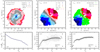 |
Fig. 5. As Fig. 4 but for the galaxy M-7975-09101. |
| In the text | |
|
Fig. 6. Panel a: comparison between the values of the inclination angle obtained from the analysis of the velocity fields, ikin, and from the analysis of the photometric maps, iphot, for our sample of MaNGA galaxies. The points stand for individual galaxies. The line indicates unity. The plus signs indicate data for CALIFA galaxies from Holmes et al. (2015). Panel b: comparison between the kinematic inclination angles derived here and the inclination angles from the HyperLeda database. Panel c: comparison between the photometric inclination angles derived here and the inclination angles from the HyperLeda database. |
| In the text | |
|
Fig. 7. Shift of the initial rotation curve (RCA) relative to the final rotation curve (RCB) as a function of rotation velocity Vrot (panel a) and as a function of the scatter in the spaxel velocities around the initial rotation curve (panel b) for our sample of the MaNGA galaxies. |
| In the text | |
|
Fig. 8. Obtained rotation curve and fit with a Polyex curve for three MaNGA galaxies. Rg is the fractional radius (normalized to the optical radius R25). In each panel, the obtained rotation curve is represented by grey circles. The bars indicate the mean scatter of the spaxel rotation velocities in rings of 1 pixel width. The solid line is the fit with a Polyex curve. The asterisk is the maximum value of the rotation velocity in the rotation curve fit within the optical radius. In panel c, the Polyex curve fit to the outer part of the rotation curve (points marked with red crosses) is presented by a dashed line and the corresponding maximum value of the rotation velocity is indicated by a square. |
| In the text | |
|
Fig. 9. Panel a: spectroscopic stellar mass of our galaxies, Msp, as a function of their photometric stellar mass, Mph. The points represent the individual MaNGA galaxies of our sample. The solid line is the linear best fit to those points. The dotted line indicates exact correpondence in the masses. Panel b: MaNGA stellar mass, Mma, as a function of photometric stellar mass, Mph, and panel c: MaNGA stellar mass, Mma, as a function of spectroscopic stellar mass Msp. The notations are the same as in panel a. Panels d–f: Mph, Msp, and Mma as a function of the rotation velocity Vrot, respectively. The points denote individual galaxies, the solid line is the Mph–Vrot relation (best fit), the long-dashed line is the Msp–Vrot relation, and the short-dashed line is the Mma–Vrot relation. |
| In the text | |
|
Fig. 10. Panel a: comparison of our Mph–Vrot relation with the stellar mass Tully–Fisher relation from McGaugh & Schombert (2015) and two relations (for two kinds of stellar mass estimates) from Reyes et al. (2011). The meaning of each line is described in the legend. Each relation is shifted along the M-axis in such a way that the log M = 10.7 at log Vrot = 2.3. Panels b and c: same as panel a but for the Msp–Vrot and Mma–Vrot relations, respectively. |
| In the text | |
|
Fig. 11. Normalized histogram of the ratios of the galactic effective radius Re, g to the point spread function PSF (full width at the half maximum) for our sample of galaxies (long-dashed line). The short-dashed line indicates the normalized histograms of the optical radius R25 to the PSF ratios. The solid line denotes the histogram of the radii (expressed in units of PSF) up to which the measurements are available. |
| In the text | |
|
Fig. 12. Panel a: stellar mass Tully–Fisher relation for our sample of MaNGA galaxies. Galaxies measured with different numbers of fibres are indicated by different symbols. Panel b: same as panel a but the galaxies with different Re, g/PSF (the ratio of the effective radius of the galaxy to the full width at half maximum of the point spread function) are indicated by different symbols. |
| In the text | |
|
Fig. 13. Spectroscopic stellar mass of our galaxies, Msp, as a function of rotation velocity, Vrot. The individual MaNGA galaxies of our sample with different values of di = ikin − iphot are shown by different symbols. |
| In the text | |
|
Fig. 14. Spectroscopic stellar mass of our galaxies, Msp, as a function of rotation velocity, Vrot. The rotation velocity along the flat part of the rotation curve, Vflat, is shown for the galaxy if this value was obtained (circles). For the other galaxies, the maximum value of the rotation velocity within optical radius is plotted (plus signs). |
| In the text | |
|
Fig. 15. Central intersect oxygen abundance 12 + log(O/H)B for the radial gradient based on the points within 0.2 < Rg < 0.8 as a function of central intersect oxygen abundance 12 + log(O/H)A for the radial gradient based on the points within Rg < 1 (circles). The plus symbols show the same for the intersect oxygen abundance at the optical radius R25. The solid line indicates equal values: the dashed lines show the ±0.05 dex deviation from unity. The oxygen abundances are determined through the R calibration. |
| In the text | |
|
Fig. 16. Panel a: comparison between central intersect oxygen abundances based on the abundances obtained through the R calibration of Pilyugin & Grebel (2016) and that based on the abundances obtained through the N2 calibration of Marino et al. (2013) (circles). The plus symbols show the comparison between intersect oxygen abundances at the optical radius R25. Circles in panel b: comparison between central intersect oxygen abundances based on the abundances obtained through the R calibration and that based on the abundances obtained through the O3N2 calibration of Marino et al. (2013). The plus symbols show the comparison between intersect oxygen abundances at the optical radius R25. Circles in panel c: abundance gradient for the N2-based abundances as a function of the abundance gradient for R-based abundances. The plus symbols show the abundance gradient for the O3N2-based abundances as a function of abundance gradient for R-based abundances. The dashed line in each panel indicates equal values. |
| In the text | |
|
Fig. 17. Panel a: nitrogen line N2 intensity vs. excitation parameter P. The circles show the positions of the spectra of the calibrating objects of different metallicities (colour-coded) from Pilyugin & Grebel (2016). The plus symbols show the positions of the MaNGA spaxel spectra with −0.600 > log N2 > −0.610 (which correspond to an N2-based abundance of 12 + log(O/H) ∼8.2). The crosses show the positions of the MaNGA spaxel spectra with 0.265 > log N2 > 0.255 (which correspond to an N2-based abundance of 12 + log(O/H) ∼8.6). Panel b: R3/N2 line ratio vs. excitation parameter P. The plus symbols show the positions of the MaNGA spaxel spectra with 1.105 > log(R3/N2) > 1.095 (which correspond to an O3N2-based abundance of 12 + log(O/H) ∼8.2). The crosses show the positions of the MaNGA spaxel spectra with −0.765 > log(R3/N2) > −0.775 (which correspond to an O3N2-based abundance of 12 + log(O/H) ∼8.6). The notations of the calibrating objects are the same as in panel a. |
| In the text | |
|
Fig. 18. Properties of our sample of galaxies. The panels show the normalized histograms of the distances to our galaxies in Mpc (panel a), rotation velocities Vrot in km s−1 (panel b), spectroscopic stellar masses Msp in solar units (panel c), luminosities LB in solar units (panel d), optical radii R25 in kpc (panel e), inclination angles i in degrees (panel f), central (intersect) oxygen abundances 12 + log(O/H)0 (solid line) and oxygen abundances at the optical radii 12 + log(O/H)R25 (dashed line) (panel g), number of points in the velocity map (solid line), and number of points used in the determination of the final rotation curve (dashed line) (panel h). |
| In the text | |
|
Fig. 19. Central oxygen abundance (O/H)0 (panel a) and the oxygen abundance at the optical radius (O/H)R25 (panel b) as a function of the rotation velocity Vrot. The grey points stand for the individual galaxies; the dark points are the binned mean values. The solid line is the broken (O/H)0–Vrot relation, and the dashed line is the broken (O/H)R25–Vrot relation. |
| In the text | |
|
Fig. 20. Left column panels: parameters X( = Msp, LB, R25, Mma; from top to bottom) as a function of the value of the rotation velocity Vrot. Middle column panels: central oxygen abundance (O/H)0 as a function of the parameters X. Right column panels: oxygen abundance at the optical radius (O/H)R25 as a function of the parameters X. The grey points on each panel represent the data for individual MaNGA galaxies from our sample; the dark points are the mean values in bins. |
| In the text | |
|
Fig. 21. Central oxygen abundance (row a panels), the abundance at the galaxy effective radius (row b panels), and at the optical radius (row c panels) as a function of the stellar mass Msp (left column panels), as a function of Msp/Re, g (middle column panels), and as a function of |
| In the text | |
|
Fig. 22. Radial abundance gradient measured in dex/kpc (left column panels), with respect to the optical radius R25 (middle column panels), and with respect to the disc scale length hd (right column panels). Row a panels: radial abundance gradient as a function of the rotation velocity Vrot, row b panels: as a function of the stellar mass Msp, row c panels: as a function of galaxy luminosity LB, row d panels: as a function of optical radius R25, and row e panels: as a function of the stellar mass Mma. The grey points at each panel are the data for individual MaNGA galaxies from our sample, while the dark points are the binned mean values. The dashed line in the middle and right column panels show the mean values of the gradient in units of dex/R25 and dex/hd, respectively. |
| In the text | |
|
Fig. 23. Radial abundance gradient measured in dex/Re, d (left column panels) and dex/Re, g (right column panels). Row a panels: radial abundance gradient as a function of the rotation velocity Vrot, row b panels: as a function of the stellar mass Msp, row c panels: as a function of galaxy luminosity LB, row d panels: as a function of optical radius R25, and row e panels: as a function of the stellar mass Mma. The grey points at each panel are the data for individual MaNGA galaxes from our sample, while the dark points are the binned mean values. The dashed line in the left and right column panels show the mean values of the gradient in units of dex/Re, d and dex/Re, g, respectively. |
| In the text | |
|
Fig. 24. Panel a: ratio of the disc scale length to the optical radius hd/R25 as a function of the value of the rotation velocity Vrot. The grey points represent the data for individual MaNGA galaxies from our sample, and the dark points indicate the binned mean values (omitting objects with hd/R25 > 0.7). The dotted line is the mean hd/R25 value. Panel b: same as panel a but for the ratio of the effective radius of the galaxy to the optical radius Re, g/R25. |
| In the text | |
|
Fig. 25. Panel a: central oxygen abundance as a function of rotation velocity for our sample of MaNGA galaxies. Depending on their angular size, the number of fibres covering the galaxies varied during the observations with the integral field units employed by MaNGA. The differing numbers of fibres are indicated by different symbols. Panel b: same as panel a but for the oxygen abundances at the isophotal radius. Panel c: central oxygen abundance as a function of stellar mass Msp. Again the different numbers of fibres are indicated by different symbols. Panel d: same as panel c but for the oxygen abundances at the isophotal radius. The value of the Msp for the galaxy measured with 37 fibres is not available. |
| In the text | |
|
Fig. 26. Oxygen abundance as a function of the spectroscopic stellar mass. The oxygen abundances at the centres of individual MaNGA galaxies with redshift z < 0.05 are shown by circles, and those for galaxies at z > 0.05 are shown by plus signs. The solid line is the O/H–Msp relation obtained for a large sample of SDSS galaxies with redshift z = 0.03 in Pilyugin et al. (2017b). |
| In the text | |
|
Fig. 27. Panel a: stellar mass as a function of redshift for our galaxy sample. The galaxies of the primary (“low redshift”) and secondary (“high redshift”) sub-samples of the MaNGA targets (Bundy et al. 2015; Wake et al. 2017) are shown by different symbols. Panel b: stellar mass Tully–Fisher relation for those galaxies. Panels c and d: central oxygen abundance (panel c) and the oxygen abundance at the optical radius (panel d) as a function of stellar mass of the galaxy. |
| In the text | |
Current usage metrics show cumulative count of Article Views (full-text article views including HTML views, PDF and ePub downloads, according to the available data) and Abstracts Views on Vision4Press platform.
Data correspond to usage on the plateform after 2015. The current usage metrics is available 48-96 hours after online publication and is updated daily on week days.
Initial download of the metrics may take a while.