| Issue |
A&A
Volume 623, March 2019
|
|
|---|---|---|
| Article Number | A179 | |
| Number of page(s) | 16 | |
| Section | Planets and planetary systems | |
| DOI | https://doi.org/10.1051/0004-6361/201833997 | |
| Published online | 02 April 2019 | |
Gas flow around a planet embedded in a protoplanetary disc
Dependence on planetary mass
1
Department of Earth and Planetary Sciences, Tokyo Institute of Technology,
Ookayama, Meguro-ku,
Tokyo
152-8551, Japan
e-mail: This email address is being protected from spambots. You need JavaScript enabled to view it.
2
Earth-Life Science Institute, Tokyo Institute of Technology,
Ookayama, Meguro-ku,
Tokyo
152-8550, Japan
Received:
1
August
2018
Accepted:
23
January
2019
Abstract
Context. The ubiquity of short-period super-Earths remains a mystery in planet formation, as these planets are expected to become gas giants via runaway gas accretion within the lifetime of a protoplanetary disc. The cores of super-Earths should form in the late stage of disc evolution to avoid runaway gas accretion.
Aims. The three-dimensional structure of the gas flow around a planet is thought to influence the accretion of both gas and solid materials. In particular, the outflow in the midplane region may prevent the accretion of solid materials and delay the formation of the super-Earth cores. However, it is not yet understood how the nature of the flow field and outflow speed change as a function of the planetary mass. In this study, we investigate the dependence of gas flow around a planet embedded in a protoplanetary disc on the planetary mass.
Methods. Assuming an isothermal, inviscid gas disc, we perform three-dimensional hydrodynamical simulations on the spherical polar grid, which has a planet located at its centre.
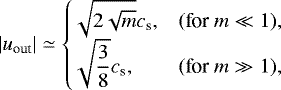
Results. We find that gas enters the Bondi or Hill sphere at high latitudes and exits through the midplane region of the disc regardless of the assumed dimensionless planetary mass m = RBondi∕H, where RBondi and H are the Bondi radius of the planet and disc scale height, respectively. The altitude from where gas predominantly enters the envelope varies with planetary mass. The outflow speed can be expressed as |uout| = √3/2mcs (RBondi ≤ RHill) or |uout| = √3/2(m/3)1/3cs (RBondi ≥ RHill), where cs is the isothermal sound speed and RHill is the Hill radius. The outflow around a planet may reduce the accretion of dust and pebbles onto the planet when m ≳ √St, where S t is the Stokes number.
Conclusions. Our results suggest that the flow around proto-cores of super-Earths may delay their growth and consequently help them to avoid runaway gas accretion within the lifetime of the gas disc.
Key words: hydrodynamics / planets and satellites: atmospheres / planets and satellites: formation / protoplanetary disks
© ESO 2019
1 Introduction
The Kepler mission has found that about 50% of Sun-like stars harbour short-period super-Earths with orbital periods of less than 85 days and radii of 1–4 R⊕ (Earth radii; e.g. Fressin et al. 2013). Radial velocity measurements and transit timing variations have also revealed that the masses of those planets are in the range of 2–20 M⊕ (Earth masses; e.g. Weiss & Marcy 2014). The reason for the ubiquity of short-period super-Earths has not been fully elucidated by planet formation theory.
According to the core accretion model, when the total mass of a planet has reached critical core mass, Mcrit ~ 10M⊕, runaway gas accretion is triggered and the planet evolves into a gas giant (e.g. Mizuno 1980; Pollack et al. 1996; Ikoma et al. 2000). The runaway timescale is about 1 Myr for a solid core of 10 M⊕, which is comparable to the typical disc lifetime of a few million years, but this timescale is much shorter when the atmosphere is dust free (Lee et al. 2014). Short-period super-Earths have avoided runaway gas accretion and growth into gas giants within the lifetime of the disc.
Hydrodynamic effects in a disc have been proposed as one solution to avoid runaway gas accretion (Ormel et al. 2015a). Gas from the protoplanetary disc enters the Bondi sphere of a planet embedded in a disc at high latitudes and leaves it through the midplane regions. The latter authors argued that the continuous recycling of atmosphere within the Bondi sphere is faster than the cooling of the envelope gas, meaning that further accretion of disc gas is prevented; though the efficiency of the atmospheric recycling is a controversial issue (Cimerman et al. 2017; Lambrechts & Lega 2017; Kurokawa & Tanigawa 2018). In addition, the dominance of disc-wind-driven accretion over viscous accretion onto the star may induce a supply limit to the gas accretion onto the cores of super-Earths (Ogihara & Hori 2018).
The late-stage core-formation model has also been suggested as another solution. In this scenario, the cores of super-Earths are assumed to have formed via coagulation of proto-cores during disc dispersal (Lee et al. 2014). The final assembly during disc dispersal is the expected result in conventional planet formation theory due to mutual gravitational interactions of proto-cores (e.g. Kominami & Ida 2002; Inamdar & Schlichting 2015). Gas accretion during the limited period before disc dispersal results in super-Earths with envelopes that make up ~1–10% of their total mass (Ikoma & Hori 2012; Owen & Wu 2016; Ginzburg et al. 2016).
The plausible late-stage core-formation scenarios involve the migration of the super-Earth cores formed at distant orbits (Tanaka et al. 2002; Ogihara & Ida 2009; Ida & Lin 2010); after forming proto-cores beyond the snow line, they begin to migrate inwards. Super-Earths form in the inner region of the disc via giant impact. This idea is supported by the inference that some of the low-density super-Earths may contain large amounts of water (Léger et al. 2004; Selsis et al. 2007; Rogers & Seager 2010; Valencia et al. 2010; Lopez & Fortney 2013; Weiss & Marcy 2014). The presence of water on the super-Earths has also been suggested from observations. From the observationsof some super-Earths – for example GJ 1214b – a featureless transmission spectrum has been found in the observed band, which suggests that the atmosphere of the planet could be dominated by relatively heavy molecules, such as water, or could contain extensive high-altitude clouds or haze (Narita et al. 2013; Kreidberg et al. 2014).
The feasibility of the late-stage core-formation scenario depends on the planet formation regimes. In the pebble accretion theory (Ormel & Klahr 2010; Lambrechts & Johansen 2012), cores accrete particles with radii of between approximately 1 mm and 1 cm drifting from the outer region of the disc. In this scenario, pebble isolation mass becomes large in the outer region of the disc,  M⊕ at 1 au (Lambrechts et al. 2014). Proto-cores can become rather heavy, which leads to runaway gas accretion and the evolution of cores into gas giants. Therefore, it is necessary to suppress pebble accretion.
The horseshoe flows extended in the anterior-posterior direction in the planet’s orbital direction have a characteristic vertical structure like a column, and a fraction of the horseshoe flow sharply descends towards the planet due to the gravity of the latter (Fung et al. 2015). These latter authors reported that outflow from the Bondi sphere at the midplane region has the speed of the order of isothermal sound speed, ~ cs. This outflow has the potential to affect the accretion of solid materials to the core of the planet and may delay its growth. The flow field around the planet affects the accretion rate of solid materials. In 2D simulations, trajectories of small solid particles vary with conditions, and accretion of these particles may be suppressed in the case of small dust-size particles (Ormel 2013). In the 3D case, small particles (10 μm–1 cm) move away from the planet in the horseshoe flow (Popovas et al. 2018).
Although there have been many previous studies with different calculation settings (isothermal or non-isothermal, inviscid or viscous, local or global frame, etc.), how the nature of the flow field changes as a function of the mass of the planet remains unclear. In this study, we therefore focus on the dependence of the flow field on planetary mass and principally investigate the speed of outflow.
The structure of this paper is as follows. In Sect. 2 we describe the numerical method. In Sect. 3 we show the results obtained from a series of simulations and present an analytic estimate of outflow speed. In Sect. 4 we discuss the implications for the formation of super-Earths. We summarise in Sect. 5.
2 Methods
In this study, we performed 3D hydrodynamical simulations of the gas of the protoplanetary disc around a planet, and investigated how the nature of the flow field changes as a function of the planetary mass. Most of our methods of the simulations followed that of Kurokawa & Tanigawa (2018); these authors focused on the differences between isothermal and non-isothermal simulations, whereas we focused on the dependence of the flow field on the planetary mass and conducted detailed studies.
2.1 Dimensionless units
The scale of the lengths, times, velocities, and densities are normalised by disc scale height H, the reciprocal of the orbital frequency Ω−1, the isothermal sound speed cs, and the gas density at planetary orbit ρdisc, respectively.In this dimensionless unit system, the dimensionless mass of the planet is expressed by the ratio of the Bondi radius of the planet, RBondi, to the scale height of the disc,
 (1)
(1)
where G is the gravitational constant, and Mp is the mass of the planet. When we assume a solar-mass star and a disc temperature profile  K, which corresponds to the minimum-mass solar nebula model (Weidenschilling 1977; Hayashi et al. 1985), Mp is described by
 (2)
(2)
where a is the orbital radius (Kurokawa & Tanigawa 2018). The dimensionless planetary mass m = 0.01 corresponds to a planet of 0.12 M⊕ revolving around a solar-mass star at 1 au (Eq. (2)).
Under this dimensionless unit, the Hill radius of the planet is given by
 (3)
(3)
and the relationships RBondi ≤ RHill and RHill ≤ H hold when m ≤ 0.58 and m ≤ 3, respectively.
2.2 Governing equations
The dimensionless governing equations for isothermal and inviscid fluid in the dimensionless unit are described as follows.
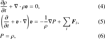
where ρ is density, t is time, v is velocity, P is pressure, and Fi is external force, respectively. Our simulations were performed on the spherical polar coordinate co-rotating with a planet at the orbital frequency Ω. Therefore, the second term in the right hand side of Eq. (5) consists of the following elements: the Coriolis force Fcor = −2Ω ×v, the tidal force Ftid = 3xΩ2ex − zΩ2ez, and the gravitational force,
![Mathematical equation: \begin{align*} \bm{F}_{\textrm{grav}}=-\nabla\Phi_{\textrm{p}}\left\{1-\exp\left[-\dfrac{1}{2}\left(\frac{t}{t_{\textrm{inj}}}\right)^{2}\right]\right\}, \end{align*}](/articles/aa/full_html/2019/03/aa33997-18/aa33997-18-eq10.png) (7)
(7)
where tinj is the injection time and Φp is the gravitational potential expressed by
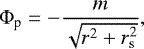 (8)
(8)
where r is the distance from the centre of theplanet, and rs is the softening length in the r-direction. We set the softening length to be equal to 7% of the Bondi radius of the planet for all simulations. Ormel et al. (2015a) reported that a rapid increase of the gravity of the planet in the unperturbed disc affects the results of the simulations. To avoid this numerical problem, the gravity of the planet is gradually inserted into the disc at the injection time, tinj.
2.3 Disc model
A planet is embedded in an isothermal, inviscid gas disc and is orbiting around the central star at the distance a with the orbital frequency  , where M* is the mass of the host star. The Bondi radius of the planet,
  , is assumed to be larger than the physical radius of the planet. In most of our simulations, RBondi was smaller than the disc scale height, H.
We consider the vertical structure of the density distribution in the disc,
![Mathematical equation: \begin{align*} \rho_{\infty}(z)=\rho_{\textrm{disc}}\exp\left[-\frac{1}{2}\left(\frac{z}{H}\right)^{2}\right],\vspace*{-4pt} \end{align*}](/articles/aa/full_html/2019/03/aa33997-18/aa33997-18-eq14.png) (9)
(9)
where ρdisc is the density of the unperturbed disc and z was the distance in the vertical direction. The density stratification is assumed to be the initial state of the disc. We set Eq. (9) as the boundary condition at the outer edge of the computational domain (see Sect. 2.4).
Keplerian shear existed in the unperturbed state of the disc and had the velocity
 (10)
(10)
where ey is the unit vector in the y-direction. We did not include the headwind of the disc (namely, the gas disc rotates in a Keplerian fashion).
2.4 Boundary conditions
Our 3D hydrodynamical simulations were performed on the spherical polar coordinates (r, θ, ϕ), which have specific boundary conditions, as described below.
Since all of our simulations were performed under the inviscid condition, we introduced the free-slip inner boundary at r = rinn to prevent the loss of mass in the radial direction, where rinn is the inner edge of the computational domain. We adopted rinn = 10−3.
We also introduced the outer edge of the computational domain at r = rout where the density and the velocity have constant values, ρ = ρ∞(z), and v = v∞(x). The choice of the domain size is justified in Sect. 3.2.1 and Appendix A. For the azimuthal direction, a periodic boundary condition was introduced such that the relationship A(r, θ, ϕ) = A(r, θ, ϕ + 2π) holds for an arbitrary scalar or vector quantity A.
We defined the simulations with the resolution [log r, θ, ϕ] = [128, 64, 128] as the fiducial models. We also performed low- and high-resolution simulations with [log r, θ, ϕ] = [100, 50, 100] and [160, 80, 160], respectively. We confirmed that the numerical convergence was achieved: the key results do not depend on resolution (see Appendix A for details). We adopted a logarithmic grid for the radial coordinate, which has a higher resolution in the vicinity of the planet.
2.5 Athena++ code
To perform our simulations, we used Athena++ code, which was a complete re-write of the Athena astrophysical magnetohydrodynamics (MHD) code (White et al. 2016; Stone et al., in prep.). Athena++ provides a Python script for reading data from output files of the calculations and, in this study, we performed various analyses using this script. In some of the results of our analysis, we averaged some components of the velocities in the azimuthal direction on the midplane of the disc (see Sect. 3). If certain components of the velocity and the density of the flow field are given as continuous functions, the weighted average velocity in the azimuthal direction is described as
 (11)
(11)
where ρgas is the gas density and vλ (λ = r, θ, ϕ) is a certain component of the velocity of gas. In a series of results obtained from our grid simulations using Athena++ code, all physical quantities were given as discrete data on grid points of each grid divided into Nr × Nθ × Nϕ = 128 × 64 × 128, where Nr, Nθ, and Nϕ refer to the number of grid sections in each direction. We set these such that each grid number in each direction is expressed as (r, θ, ϕ) = (i, j, k), and since j = 32 corresponds to the midplane of the disc, a certain component of the velocity on an arbitrary grid is represented by  . Therefore, azimuthally averaged velocity on the ith grid was calculated by
 (12)
(12)
where  and
and  are the density and the λ-component of the velocity on the arbitrary coordinate has the grid number (i, j, k).
2.6 Parameter sets
All of our simulations are listed in Table 1. When the Hill radius of the planet exceeds the size of the disc scale height (m > 3), a gap formsclose to the planet’s orbit in a disc (Lin & Papaloizou 1993). Our local simulations, however, could not handle the gap opening. For this reason we only handled a range of planetary masses, m = 0.01–2, in a series of simulations.
Through performing test simulations several times, we confirmed that an unphysical flow pattern emerged in the vicinity of the planet in the early stage of the time evolution of the flow field when tinj was short, especially for planets with m ≥ 0.5. Therefore, we set the length of the injection time to be longer for the planets with m ≥ 0.5. We also found that it takes a longer time for the flow field to reach the steady state, particularly for the planets with m ≥ 0.05. Accordingly, we set the tend long enough for the flow field to reach the steady state in all of our simulations.
3 Results
The main subject of this study is to clarify the dependence of the gas flow field on planetary mass. As a result of a series of simulations, there were some properties that varied depending on the mass of the planet and others that did not. In Sect. 3.1, we show universal properties of the flow field that are independent of the planetary mass. Section 3.2 shows the dependence of the flow field on the planetary mass.
Simulations.
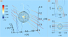 |
Fig. 1 3D structure of the flow field obtained from m1 run at t = 100. The solid lines and the sphere represent the characteristic streamlines of gas flow around the planet and the Bondi region, respectively. The colour shows the radial velocity normalised by the isothermal sound speed. The regions where vr has a positive (outflow) or a negative value (inflow) are shown in blue and red, respectively. Panel a: perspective view of the flow field. Panel b: x–y plane viewedfrom the + z direction. Panel c: y–z plane viewedfrom the − x direction. |
3.1 The structure of the gas flow field
Through performing 3D hydrodynamical simulations, we found the characteristic structures of the flow field around the planets. Figure 1 shows the 3D structure of the flow field around the embedded planet obtained from calculation of the m1 run at t = 100. Figure 1a is a bird’s-eye view of the flow field. Figure 1b and c are the x–y plane viewed from the + z direction and the y–z plane viewed from the − x direction, respectively. A planet is located at the centre of the Bondi sphere which is expressed by the black solid lines in each panel. The structure of the flow is consistent with previous studies (Ormel et al. 2015a; Fung et al. 2015; Cimerman et al. 2017; Lambrechts & Lega 2017; Kurokawa & Tanigawa 2018). Gas flows in at high latitudes of the Bondi sphere of the planets and leaves through the midplane of the disc. The flow field has three types of streamlines defined as follows.
The Keplerian shear streamline
The Keplerian shear exists near x ≳ 1.5 and extends in the y direction (Figs. 1a and b). These streamlines are slightly perturbed by the gravity of the planet however, and do not accrete onto the planet.
The horseshoe streamline
The horseshoe flow exists in the anterior-posterior direction of the orbital path of the planet (Figs. 1a and b). The streamlines show a columnar structure as reported in Fung et al. (2015). In all of our simulations, we found the horseshoe flow to have a similar vertical structure. The streamlines that are relatively close to the planet underwent a gravitational perturbation by the planet and descended somewhat towards it, but they escaped from the Bondi sphere of the planet without reaching it.
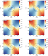 |
Fig. 2 Time evolution of the flow field around a planet with m = 1.0 at the midplane of the disc. Each panel corresponds to the snapshots at t = 2, 3, 5, 10, 50, and 100. Since we set the injection time to unity, in this run, the gravity of the planet has been completely inserted into the disc in all panels. Colour contour represents the flow speed in the radial direction. The vertical and horizontal axes are normalised by the scaleheight of the disc. The solid and dashed lines correspond to the specific streamlines and the Bondi radius of the planet, respectively. Blue and red regions imply where the gas flows inwards and outwards. After accretion phase (t < 2), gas flowing from the centre of the planet (outflow) emerges in the early stage of the time evolution. The topologies of the flow field have not significantly changed after t = 5 in this simulation. We note that the length of the arrows does not scale with the flow speed. |
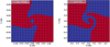 |
Fig. 3 Structure of the inflow and outflow in the region close to the planet at the midplane. Panel a: result obtained from m01 at t = 50. Panel b: result obtained from m1 at t = 100. In order to distinguish the inflow and outflow clearly, we plotted vr∕|vr|. Red and blue correspond to the regions where vr∕|vr| has positive and negative values. We note that the length of the arrows does not scale with the flow speed. |
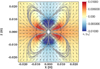 |
Fig. 4 Vertical structure of inflow and outflow at the meridian plane (y = 0) obtained from m001 at t = 10. The red andblue regions correspond to areas where gas flows outwards and inwards in the radial direction, respectively. The solid and dashed lines represent the specific streamlines of gas flow and the Bondi radius of the planet, respectively. The contourhas the same meaning as that in Fig. 2, but the ranges are different. Since we adjusted the range of thecontour to show the vertical structure of the outflow, the value of inflow is saturated in the vicinity of the planet. We note that the length of the arrows does not scale with the flow speed. |
The atmospheric recycling streamline
A few streamlines reach the vicinity of the planet (Figs. 1a–c). These streamlines start to descend halfway along the horseshoe orbit. After entering directly above the planet however, they sharply descend towards it. Subsequently, they circle the planet several times and one of them ultimately exits the Bondi sphere through the midplane region of the disc. The altitude where the gas begins to descend is approximately two times higher than the top of the Bondi sphere. This streamline connects inside and outside the Bondi sphere. Therefore, this embedded atmosphere represents an open system where gas continuously enters the Bondi sphere and leaves it (Ormel et al. 2015a).
The outflow emerged from the early stage of the time evolution. Figure 2 shows the time evolution of the flow field at the midplane of the disc. A planet is located at the centre of this figure. At the early stage of the time evolution of the flow field, gas accretes onto the planetary core (as shown in Fig. 2a). After the accretion phase, the gas begins to circulate in the vicinity of the core of the planet. As shown in Fig. 2a, inflow (represented in blue) is dominant inside the Bondi sphere at t < 3.
The situation changes after t = 3. In Figs. 2b–f, there are three types of streamlines: the Keplerian shear streamlines, the horseshoe streamlines, and the atmospheric recycling streamlines. The Keplerian shear exists on both the left and right sides of the planet. Although it is slightly distorted due to the gravity of the planet, its trajectory is almost straight without accreting onto the core of the planet. Horseshoe flows are rotationally symmetric with respect to the z-axis. Part of the horseshoe flow enters the Bondi sphere of the planet and exits it, drawing a U-turn curve without accreting onto the core of the planet. Atmospheric recycling streamlines connect inside and outside the Bondi sphere of the planet. In this phase, the topology of the flow field does not change significantly with time in the m1 run. The shape of thestreamlines experiences only a slight change in the vicinity of the planet. A similar trend was also confirmed regardless of the assumed planetary mass. After the accretion phase, the flow field approached the steady state.
What is striking about Fig. 2 is that the gas flows out from the core of the planet towards an area outside the Bondi region, travelling along the horseshoe streamlines or atmospheric recycling streamlines at the midplane of the disc. Other simulations assuming different planetary masses show similar tendencies of the outflow of gas from the vicinity of the planet. In Fig. 2, the speed of outflow near the Bondi radius has reached the order of the isothermal sound speed. Such a fast flow of gas at the midplane of the disc has the potential to affect the solid materials around the planet. If the outflow speed is high compared to the radial drift speed of the solid materials, it is probable that outflow behaves as a barrier against the accretion of solid materials and suppresses the accretion rate.
In the region close to the planet, the radial outward flow is dominant (Figs. 3a and b). We confirmed the dominance of outflow in the midplane in the vicinity of the planet in all of our simulations. When m ≤ 0.58 (RBondi < RHill), inflow emerged only at r ≳ 0.1–0.2 RBondi (Fig. 3a). Although inflow tails intrude deep inside the Bondi sphere when m ≥ 0.58 (RBondi > RHill), their width is narrow (Fig. 3b). The outflow in the midplane near the planet is expected to reduce the accretion of solid materials (see Sect. 4.3).
Figure 4 shows the vertical structure of inflow and outflow at the meridian plane, y = 0. The solid lines are the specific streamlines and they have an axisymmetric structure. Gas flows in from the vertical direction of the z-axis and escapes near the midplane to mid-latitudes of the disc. In this figure, the gas seems to be descending from a height twice as high as the top of the Bondi sphere or more. Some of the streamlines correspond to the outflow circulating inside the Bondi sphere. The vertical scale of the outflow is about 0.5 RBondi. The vertical scale of the outflow is important because the influence on the dust or pebble accretion would be determined by the ratio of the vertical extent of the flow to the scale height of the solid materials.
The fundamental features of the flow field introduced above were not changed significantly with planetary mass.
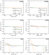 |
Fig. 5 Azimuthally averaged mass flux, |


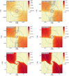 |
Fig. 6 Changes of the outflow speed at the midplane of the disc according to the planetary mass. Each panel corresponds to each result obtained from different simulations at t = tend. Colour contour represents the flow speed in the radial direction. In order to show the differences of the outflow speed specifically, we plotted in a logarithmic scale. We note that the colour contour is saturated for the inflow (vr < 0) region. The orange-red and yellow areas mostly correspond to the regions where the radial velocity is positive or negative, respectively (see Fig. 2). The solid lines correspond to the specific streamlines of the gas flow. The black dashed line corresponds to the Bondi radius of the planet. The green dashed line shown in panels e and f corresponds to the Hill radius. We note that the length of the arrows does not scale with the flow speed. |
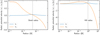 |
Fig. 7 Azimuthally averaged radial and azimuthal velocity as a function of the radius r. Left panel: result from m005 run at t = 30. Right panel: result from m2 run at t = 100. The solid lines correspond to the radial (blue) and azimuthal (orange) velocity of the gas flow in the vicinity of the planet. The dashed line shows the position of the Bondi or Hill radius of the planet. |
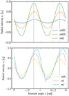 |
Fig. 8 Changes of the radial velocity in the azimuth direction at the Bondi (for m001, m005, m01, m05) or Hill radius (for m1, m2) on the midplane of the disc at t = tend. The solid lines correspond to each analytical result obtained from each simulation. Each dashed line corresponds to the locations where ϕ = 3π∕4, 7π∕4. The radial velocity reaches its maximum value near these points after it takes the periodic oscillation. The maximum value of vr increases with the planetary mass. Positive or negative values of vr refer to where inflow or outflow emerges. |
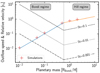 |
Fig. 9 Outflow speed as a function of dimensionless planetary mass. The cross symbols are the maximum value of the outflow speed at the Bondi (for m001, m005, m01, m05) or Hill radius (for m1, m2) on the midplane of the disc obtained from our simulations at t = tend. The blue and orange solid lines correspond to the analytical solution of the outflow speed derived from Eqs. (17) and (18), which are divided at the point where the size of the Bondi radius of the planet exceeds the size of the Hill radius (see Sect. 3.3 for details). Each black lineshows the changes of the relative velocity of the small particles for each Stokes number, St = 10−3 (dashed-dotted line), 10−2 (dotted line), and 10−1 (dashed line) derived from Eqs. (24) and (25); (see Sect. 4.3 for details). |
3.2 Dependence on planetary mass
3.2.1 Positions of inflow and outflow
The height of the starting point of gas falling increased with the planetary mass, due to the gravity of the planet becoming stronger. The width of the horseshoe streamline also widened with increasing planetary mass, and this tendency was consistent with the result of Fung et al. (2015).
When we analysed the velocity of the flow field around the planets, especially the estimation of the speed of outflow (described later in Sect. 3.3), it was necessary to judge where the gas chiefly flowed in and out. Figure 5 shows the azimuthally averaged mass flux,  , as a function of the altitude, z. The altitudeis changed along with the characteristic spherical surface: the Bondi sphere (blue), the Hill sphere (orange), twice the size of the Bondi sphere (green), and twice the size of the Hill sphere (red), respectively. Inflow and outflow are balanced in each region where
  . As shown in Fig. 5, the maximum and the minimum value of the azimuthally averaged mass flux decreases with increasing radius. Azimuthally averaged mass flux has the maximum value at the midplane of the disc and the minimum value at the zenith of the Bondi (for m001, m005, m01, m05) or Hill region (for m1, m2). Though Fig. 4 shows that gas flows in at a considerably high altitude (about twice as high as the Bondi radius of the planet), the quantitative analysis of the azimuthally averaged mass flux tells us that gas mainly flows in and out of whichever is smaller: the Bondi or Hill radius.
In m001,m005, and m01 runs, we set the size of the outer boundary to be smaller than the disc scale height. As shown in the enlarged view in the lower right corner of Figs. 5a–c, the dominant mass flux occurs at the position of the Bondi radius (blue solid line). In the outer region of the Bondi sphere, mass fluxes are almost zero (orange and green solid lines). Therefore, when the planetary mass is small, the materials that exist outside the Bondi radius hardly accrete and do not contribute to the changes of the flow field. We confirmed the validity of these arguments through the results of m001-extendD, m005-extendD, and m01-extendD runs whose domain sizes were taken to be larger than m001, m005, and m01 runs (see Appendix A for details). These results justify our assumption on the domain sizes.
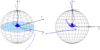 |
Fig. 10 A single specific streamline of gas flow from m005 run at t = 10. The sphere in this figure represents the Bondi sphere of the planet. The blue solid line indicates the streamline which enters at the zenith of the Bondi sphere of the planet and circles around the planet several times, finally exiting near the midplane of the disc, which is coloured light blue. For convenience when plotting a streamline, the inflow point is located at (x, y, z)= (0.001, −0.001, 0.05), which is slightly different from P1 = (0, 0, 0.05; see Sect. 3.3). |
3.2.2 The outflow speed
The speed of outflow near the Bondi or Hill radius at the midplane of the disc increases with planetary mass (Fig. 6). The topologies of the flow field are slightly different in each of the panels (a–f), especially in the vicinity of the planet, but each panel has an equal amount of each of the three types of streamlines: the Keplerian shear streamlines, the horseshoe streamlines, and the atmospheric recycling streamlines (the universal nature of the flow field was discussed in Sect. 3.1). The flow field seems to have reached a steady state. In all simulations, the maximum and the minimum values of the radial velocity show very little change over time in the late stage of the time evolution. The time until the flow field reaches the steady state was found to be longer for planets of greater mass. Whether or not the flow field has reached a steady state becomes important in deriving the analytic solution of the outflow in Sect. 3.3.
In this study, we defined the outflow region as the section where the radial velocity was dominant in the flow field near the planet compared to the azimuthal velocity; that is, a condition of vr > vϕ was set for the definition of the outflow. Figure 7 shows where the effective outflow emerges. The solid lines are the azimuthally averaged radial and azimuthal velocity of gas,  and
and  , as a function of the radius, r. In the left panel, the radial velocity exceeds the azimuthal velocity near the Bondi radius. On the other hand, for the m2 run at t = 100 shown in the right panel, the radial velocity surpasses the azimuthal velocity near the Hill radius of the planet. We also analysed other results of simulations and found that the outflow emerged from the smallest radius of the Bondi and Hill radii. These results are consistent with the analysis of the results of the azimuthally averaged mass flux, which shows where the dominant gas outflow was located (Fig. 5).
The effective outflow speed has a maximum value at ϕ ~ 3π∕4, 7π∕4 (Fig. 8). Inflow or outflow occurs where vr is positive or negative. In the 2D simulation, it is expected that the inflow and the outflow speeds will be the same in the midplane (Ormel et al. 2015b). Figure 8 shows however that the maximum and the minimum values of the radial velocity are different.
The dependency of the outflow speed on the planetary mass is presented in Fig. 9. We also plot the maximum value of the effective outflow speed at the smaller radius of the Bondi and Hill radii on the midplane of the disc obtained from the analysis of the results (Fig. 8). When the dimensionless planetary mass is smaller than unity, it seems that the outflow speed increases in proportion to the first power of the planetary mass. However, once the dimensionless planetary mass exceeds unity, the power-law index in Fig. 9 becomes less than unity. How is the outflow speed actually expressed as a function of the planetary mass? An analytical derivation of the outflow speed is presented below.
3.3 Analytical estimation of the outflow speed
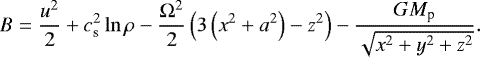
The analytical solution of the outflow speed was derived from Bernoulli’s theorem. Assuming u is the gas velocity in the rotating frame, under the isothermal and inviscid condition, Bernoulli’s function is described as
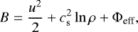 (13)
(13)
where Φeff is the effective potential expressed by
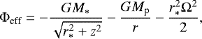 (14)
(14)
where r* is the distance from the centre of the central star. The first to the third terms in the right hand side of Eq. (14) correspond to the gravitational potential of the star, the gravitational potential of the planet, and the centrifugal potential, respectively. When this effective potential is linearly approximated with r* = a + x and |x|, |z|≪ a, Bernoulli’s function can be rewritten as
 (15)
(15)
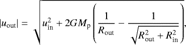
We picked up a streamline of the recycling flow (Fig. 10). We set two points on the streamline, P1 = (0, 0, z1) and  . These two points correspond to where gas flows in and out. We assume that inflow has the velocity u = uin at P1 and outflow also has the velocity u = uout at P2. Since Bernoulli’s function has the same value in the steady state at each point of P1 and P2, outflow speed can be described as
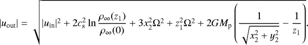 (16)
(16)
The second and fourth terms in the right-hand side of Eq. (16) would be cancelled because the stellar gravitational potential energy balances lnρ in hydrostatic equilibrium.
We defined Rin = z1 and  for convenience, which is equal to the distance from the centre of the planet where gas flowed in and out. Since we found that gas chiefly flowed in and out from the smaller of the Bondi and Hill regions – that is, the distance of the inflow and outflow point from the centre of the planet was the same – Rin = Rout. Therefore, the fifth term is also eliminated. In this case, Eq. (16) shows the relation |uout| > |uin| and gives the upper limit of the outflow speed. From the analysis of the kinetic energy of gas flow in our simulations, we found the contribution of |uin |2 was negligible at P1. Consequently, the tidal potential term determines the outflow speed uout in Eq. (16).
We defined the Bondi and Hill regimes depending on the dimensionless planetary mass. The boundary was located at m = 0.58 where the size of the Bondi sphere of the planet exceeds the size of the Hill sphere. In the Bondi regime, m < 0.58 since the effective outflow leaves the Bondi sphere near the midplane of the disc and has the maximum value at  ; Eq. (16) gives
 (17)
(17)
In the Hill regime, m > 0.58; using a similar procedure we set  and using Eq. (16) we obtain,
 (18)
(18)
Our analytic approximate solutions of the outflow speed are plotted in Fig. 9. The outflow speed increases with the dimensionless planetary mass. The power-law index depends on the regimes. The analytical estimate is found to reproduce the results of our simulations. Since Bernoulli’s theorem is applicable only to the steady flow, the agreement is consistent with the inference that our simulations at t = tend have reached a steady state. We note that the expression of uout (Eqs. (17) and (18)) represents the outflow speed not at an arbitrary point along the recycling streamline, but at a specific point where  , because we assumed Rin = Rout.
The outflow speed was similar to that of the local Keplerian shear, especially in the Bondi regime. However, one slight difference is that the local Keplerian shear velocity is expressed by vshear = −3∕2xΩ, where x is the position in the radial direction and Ω is the Keplerian frequency. By substituting  which corresponds to the outflow point, we obtain
  . Therefore, the outflow speed in the Bondi regime is slightly faster than the local Keplerian shear velocity.
We measured the outflow speed at r = min(RBondi, RHill) because this scale gives the size of the region where the flow is largely influenced by the gravity of the planet. However, the outflow extends beyond r = min(RBondi, RHill) and the speed can be estimated by Eq. (16; Appendix B).
4 Discussion
4.1 Application to the non-isothermal simulations
Our method of estimating the outflow speed is expected to be applicable to non-isothermal simulations. Under isothermal conditions, previous studies and our results have shown that gas enters at high latitudes of the Bondi or Hill sphere of the planet and leaves it through the midplane region of the disc (Ormel et al. 2015a; Fung et al. 2015; Kurokawa & Tanigawa 2018). However, non-isothermal simulations suggest different trends. A region emerges where a part of the gas is bound around the core of the planet. Three-dimensional radiation-hydrodynamical simulations on the global frame have been used to identify the interface dividing the materials bound and unbound by the planet, lying at ~ 0.4 RBondi in 5–10 au runs for m = 0.08–0.25 (D’Angelo & Bodenheimer 2013). By conducting 3D radiation-hydrodynamical inviscid simulations for m = 0.04, 0.38, 0.75, and 1.9 planets, Cimerman et al. (2017) indicated that there are no out-spiralling streamlines in the midplane corresponding to the outflow streamline as shown in Fig. 8 of Ormel et al. (2015a) or our Fig. 10. Instead, streamlines circulate close to the planet. The opacity of the disc also affects the structure of the envelope (Lambrechts & Lega 2017).The 3D radiation-hydrodynamical simulations of these latter authors on the global frame with the opacity κ = 0.01 cm^2 g^-1 found a three-layered structure inside the envelope consisting of the advection layer in the outer layer, the radiative layer in the middle layer, and the convection layer in the inner layer. These differences between isothermal and non-isothermal calculation results come from the buoyancy barrier in the envelope (Kurokawa & Tanigawa 2018). These latter authors performed two types of 3D hydrodynamical simulations on the local grid: isothermal and non-isothermal cases. In the case of non-isothermal simulations, the inflow is prevented from reaching the deep part of the envelope because buoyant force suppresses intrusion of high-entropy gas into the low-entropy atmosphere when the atmosphere starts cooling.
In the non-isothermal simulations, though the atmospheric recycling has only been observed outside the isolated inner envelope, it has not completely disappeared (Kurokawa & Tanigawa 2018). We derived the analytical solution of the outflow speed from Bernoulli’s theorem along an atmospheric recycling streamline under the isothermal condition. In the non-isothermal case, the form of Bernoulli’s function has to be changed according to the conditions. As long as the atmospheric recycling has not completely disappeared, it is expected that our method can be applied even in non-isothermal simulations. However, it is possible that the gas inflow and outflow points may change, and further studies on the current topic are therefore required.
4.2 Comparison to the analytic solution of Fung et al. (2015)
The analytical solution shown in Sect. 3.3 differs from that of Fung et al. (2015). In their study, the outflow speed was given as
 (19)
(19)
and approximately expressed by
 (20)
(20)
where the contribution of  was neglected. Equation (20) predicts that when the planetary mass is quite small, m ≪ 1, the outflow speed increases with the planetary mass; but after that, the outflow speed remains constant as the planetary mass is sufficiently large. The maximum value of the outflow speed is about uout ≃ 0.6cs. However, these analytic solutions are inconsistent with our simulation results. Our results show that the outflow speed can be slower inthe Bondi regime and faster in the Hill regime than their prediction (Fig. 9). The differences between Eqs. (17) and (18) and Eq. (20) originate from the following factors.
The use of Bernoulli’s theorem: in Fung et al. (2015), Bernoulli’s theorem was applied along with a certain horseshoe streamline. On the other hand, we applied Bernoulli’s theorem for an atmospheric recycling streamline by assuming that gas entered at the zenith of the Bondi or Hill sphere. Alternatively, they assumed that inflow and outflow only have an x- and a y-component, u = (ux, 3∕2xΩ, 0) where 3∕2xΩ is derived from the local Keplerian shear; we did not assume the components of the inflow and outflow (see Appendix of Fung et al. 2015 for details).
Configurations of inflow and outflow points: assumptions in regards to the altitude where the gas begins to descend were also different. Fung et al. (2015) considered the possibility that gas starts falling from the disc scale height, Rin≈ H. From the above-mentioned discussion (Sect. 3.2.1), we found gas mainly entered or exited whichever Bondi or Hill region of the planet was smaller. In this study we assumed the height of the falling point was the Bondi or Hill radius, Rin = min(RBondi, RHill). Though Fung et al. (2015) also assumed that the distance of the outflow point from the centre of the planet, Rout, scales with the half-width of the horseshoe orbit for the low mass limit, m ≪ 1, and scales with the Hill radius for the high mass limit, m ≫ 1, we assumed the outflow point was located at the Bondi or Hill radius, Rout = min(RBondi, RHill).
Therefore, our analytic approximate solution of the outflow speed was different from that of Fung et al. (2015)1. Since the inflow and outflow points are different from those of Fung et al. (2015), it is difficult to compare our results to theirs any further.
4.3 Implications for the formation of super-Earths via pebble accretion
We propose that the ubiquity of super-Earths may be explained by their late-stage formation due to the outflow barrier: the recycling outflow prevents dust and pebbles from accreting onto their proto-cores. In the pebble accretion theory (Ormel & Klahr 2010; Lambrechts & Johansen 2012), proto-cores can grow to a mass heavy enough to carve a gap in the pebble disc, which is given by (Lambrechts et al. 2014)
 (21)
(21)
This mass islarge enough to allow disc gas to accrete in a runaway fashion within the lifetime of a protoplanetary disc (Lee et al. 2014).
Simulations in previous studies and in this one have shown that a planet embedded in a protoplanetary disc induces outflow in the midplane region. The particle scale height is given by (Youdin & Lithwick 2007),
 (22)
(22)
where S t is the dimensionless Stokes number and α is the viscosity parameter (Shakura & Sunyaev 1973). Assuming St ~ 10−2–10−1 and α ~ 10−4–10−2 gives Hd ∕H ~ 10−2–100. Because the vertical scale of the outflow is estimated to be a few tens of percent of the Bondi radius (Fig. 4), planets with a dimensionless mass m = RBondi∕H > 10−2–100 have the potential to prevent pebbles from accreting onto them. In 2D cases, the flow field around a planet has been shown to influence the accretion rate of particles (Ormel 2013).
Three-dimensional adiabatic hydrodynamical simulations of gas and particle dynamics has shown that particles that entered the Hill sphere of the planet later exited it on the outer-trailing horseshoe flow (Popovas et al. 2018). These latter authors reported that the dominant inflow of the particles is relevant to the inner-trailing and outer-leading horseshoe flow, and dominant outflow relates to the outer-trailing and inner-leading horseshoe flow. In the Bondi region, the larger particles (> 0.1 cm) are rapidly accreted onto the planet whose mass is m = 0.011, 0.037, and 0.07. However, since the outer-trailing horseshoe flows are strong enough to carry out the smaller particles (< 0.1 cm), they do not accrete onto the planet.
We compared the outflow speed to the terminal velocity of particles within the Bondi or Hill radius in order to discuss the influence of the outflow on the core growth. Given the force balance between the gas drag and the gravity of the planet acting on the particle,
 (23)
(23)
where Δv is the terminal speed of the particle relative to the gas, and tstop is the stoppingtime expressed by tstop = St∕Ω.
In the Bondi regime, we substituted r = RBondi into Eq. (23) and obtained
 (24)
(24)
In the Hill regime, we obtained
 (25)
(25)
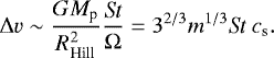
We plotted the changes of the relative velocity of the small particles as a function of the dimensionless planetary mass for each Stokes number, St = 10−3, 10−2, and 10−1 in Fig. 9. As shown in this figure, the flow field around the planets may affect the accretion of the small particles when the outflow speed exceeds the relative velocity of the particles. Planetary mass with the potential to affect the accretion can be written as  . The width of the outflow is wider than that of inflow in the midplane region near the Bondi or Hill radii (see Figs. 2and 6). It is expected that the outflow reduces the accretion of solid materials onto the planet if they enter the Bondi or Hill sphere from the outflow regions.
Even if the solid particles enter the Bondi or Hill sphere from the inflow region, the accretion onto the planet may be prevented by the flow inside the sphere. As shown in Fig. 3, outflow is dominant in the region close to the planet. The solid materials supplied from the inflow window of the Bondi or Hill sphere may be transported outwards by the outflow and are ultimately ejected from the envelope. The dense and hot envelope in the vicinity of the planet may also induce the disruption and vapourisation of solid particles, which would further prevent accretion onto the planet (Alibert 2017), though the inner part of the envelope may be isolated from the recycling flow (Kurokawa & Tanigawa 2018). Furthermore, even the particles with a relatively large Stokes number (defined at the Bondi or Hill radius) – for instance St > m2 – may also be affected by the outflow within the Bondi or Hill sphere. Since the Stokes number is inversely proportional to the gas density both in the Epstein and Quadratic regimes (e.g. Ormel & Klahr 2010), the effective Stokes number is considered to decrease inside the envelope where gas density is much higher than that of the background. In such cases, the particles become more susceptible to the outflow barrier.
Our results suggest that the flow in the vicinity of proto-cores would delay the formation of super-Earth cores and consequently help them to avoid the runaway gas accretion within the lifetime of the disk. We propose a plausible scenario for the formation ofsuper-Earths as follows.
- 1.
Proto-cores form in the outer region (~1 au) of the disc under the influence of the flow field. Due to the outflow barrier, the growth of proto-cores may halt when
 .
. - 2.
When the growth of the proto-cores halts, they begin to migrate inwards. A number of proto-cores are arranged at the inner edge of the disc.
- 3.
Super-Earths are formed by giant impact during disc dispersal. In a short time, until the gas has dissipated, an envelopeforms around each super-Earth, which has 1–10% of its mass.
In either case, further studies of the interaction between the planet-induced wind and solid materials are needed to understand the consequences on the formation scenarios of super-Earths.
5 Conclusions
We investigated gas flows around an embedded planet in a protoplanetary disc and the dependency of the flow field on the planetary mass. We considered isothermal, inviscid gas flow, and performed a series of 3D hydrodynamical simulations on a spherical polar grid that had a planet placed at its centre. We summarise our main findings as follows.
- 1.
The 3D structure of the flow field did not change significantly even if we changed the mass of the planet. Gas entered at high latitudes of the Bondi or Hill sphere and left it through the midplane of the disc, which is consistent with previous works (Ormel et al. 2015a; Fung et al. 2015; Cimerman et al. 2017; Lambrechts & Lega 2017; Kurokawa & Tanigawa 2018). The flow field had three types of streamlines: the Keplerian shear streamlines, the horseshoe streamlines, and the atmospheric recycling streamlines.
- 2.
Gas flowed in and out substantially from the smaller of the Bondi and Hill regions. Azimuthal averaged mass flux increased with the mass of the planet; it had a maximum peak at the midplane of the disc, and a minimum value at the zenith of the Bondi or Hill sphere.
- 3.
Outflow speed increased with planetary mass. Under isothermal circumstances, we derived an analytical solution for the outflow speed from Bernoulli’s theorem. Our equation predicted that the following relations held: (RBondi < RHill):
 for the Bondi regime, and (RBondi > RHill):
 for the Hill regime. These predictions were consistent with the results of numerical simulations.
 - 4.
Comparing these analytic solutions and the relative velocity of the small particles, we estimated the dimensionless planetary mass with the potential to affect the accretion of solid materials to be
 . As the mass of the planet increased, the outflow became fast and would start to prevent solid materials from accreting onto the core.
Our results suggest that the flow field around a planet has the potential to affect the accretion rate of solid materials. It is possible that the outflow barrier could inhibit the accretion of small particles. This mechanism may delay the growth of the solid core of the planet and may be helpful to explain the formation of super-Earths.
Acknowledgements
We thank Athena++ developers: James M. Stone, Kengo Tomida, and Christopher White. The authors are grateful for the constructive feedback from an anonymous referee. This study has greatly benefited from fruitful discussions with Chris W. Ormel, Michiel Lambrechts, and Anders Johansen. H.K. was supported by JSPS KAKENHI Grant number 16H04073, 17H06457, and 18K13602. S.I. was supported by JSPS KAKENHI grant 15H02065. Numerical computations were in part carried out on Cray XC30 at Earth-Life Science Institute and at the Center for Computational Astrophysics, at the National Astronomical Observatory of Japan. This research was supported by a grant from the Hayakawa Satio Fund awarded by the Astronomical Society of Japan.
Appendix A Dependence on computational resolution and domain size
To investigate the effect of numerical configuration on the main result and confirm the numerical convergence, we performed simulations with the extended domain size and with the lower or higher resolution ([logr, θ, ϕ] = [100, 50, 100] or [160, 80, 160]). All of our simulations are listed in Table 1.
As shown in Fig. A.1, the gas density obtained by fiducial (solid lines), low- (dashed lines), and high-(dotted lines) resolution simulations agree with one another.
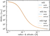 |
Fig. A.1 Gas density in the radial and vertical directions as a function of the radius, r, and altitude, z. These results are obtained from m01, m01-low, and m01-high runs at t = 30. The solid, dashed, and dotted lines correspond to the radial (blue) and vertical (orange) gas density around the planet obtained from the fiducial, low, and high resolution simulations, respectively. In the radial direction, we plotted the azimuthally averaged gas density. In the vertical direction, we plotted the gas density along the z-axis. |
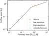 |
Fig. A.2 Maximum value of the outflow speed at the Bondi (for the planets with m = 0.01, 0.05, 0.1, and 0.5) or Hill radius (for the planets with m = 1.0 and 2.0) on the midplane of the disc obtained from the fiducial (red), low-resolution (yellow), high-resolution (green), and extended-domain (blue) simulations at t = tend. The black solid line corresponds to the analytical solution of the outflow speed derived from the analytical solution of the outflow speed derived from Eqs. (17) and (18). |
The maximum outflow speed at the midplane of the disc also matched. Figure A.2 shows the results obtained by a series of fiducial, low-resolution, high-resolution, and extended-domain simulations. Although there are slight differences in the results of the three simulations, the outflow speed obtained from simulations with different resolutions or domain sizes are also consistent with our analytic solution plotted by the black solid line.
From these results, we concluded that all of our hydrodynamical simulations reached numerical convergence and our choice of the domain size does not affect the main results.
Appendix B The application of analytic solution
Because the Bernoulli’s principle is valid along a streamline in the steady state, the outflow speed beyond r = min(RBondi, RHill) can be estimated from Eq. (16).
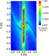 |
Fig. B.1 The colour contour shows the difference of flow speed from the Keplerian shear obtained by m05 run at t = tend. We plotted |v − v∞(x)|∕|v∞(x)|, where v is the gas velocity and v∞(x) is the Keplerian shear expressed by Eq. (10). The contour shows that the spherical region around the planet is highly influenced by the gravity. We note that the red region along x = 0 is not the outflow but the horseshoe flow. We also note that the colour contour is saturated in the region coloured with red. The grey solid lines correspond to the specific gas streamlines. We highlighted the atmospheric recycling streamline in the thick white solid line. The red, orange, green, blue, and purple dashed lines are the circles of radius RBondi, 1.5 RBondi, 1 [H], 2 [H], and 3 [H]. |
Figure B.1 shows the difference of flow speed from the unperturbed Keplerian shear. In this study, we measured the speed of planet-induced outflow at r = min(RBondi, RHill) because thisscale gives the extent of the flow influenced by the planet gravity. The outflow extends up to two to three times r = min(RBondi, RHill) and merges withthe shear flow.
Figure B.2 shows the flow speed measured at different r. Here we assumed that the gravity and density terms cancelled and that |uin|2 was negligible. The results confirm that the outflow accelerates beyond 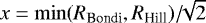 following Eq. (16).
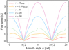 |
Fig. B.2 Flow speed obtained by m05 run as a function of azimuth angle at different r and t =tend. The cross symbols coloured by red, orange, green, blue, and purple correspond to the flow speed estimated by Eq. (16), |
References
- Alibert, Y. 2017, A&A, 606, A69 [NASA ADS] [CrossRef] [EDP Sciences] [Google Scholar]
- Cimerman, N. P., Kuiper, R., & Ormel, C. W. 2017, MNRAS, 471, 4662 [NASA ADS] [CrossRef] [Google Scholar]
- D’Angelo, G., & Bodenheimer, P. 2013, ApJ, 778, 77 [NASA ADS] [CrossRef] [Google Scholar]
- Fressin, F., Torres, G., Charbonneau, D., et al. 2013, ApJ, 766, 81 [NASA ADS] [CrossRef] [Google Scholar]
- Fung, J., Artymowicz, P., & Wu, Y. 2015, ApJ, 811, 101 [NASA ADS] [CrossRef] [Google Scholar]
- Ginzburg, S., Schlichting, H. E., & Sari, R. 2016, ApJ, 825, 29 [NASA ADS] [CrossRef] [Google Scholar]
- Hayashi, C., Nakazawa, K., & Nakagawa, Y. 1985, in Protostars and Planets II, eds. D. C. Black, & M. S. Matthews (Tucson, AZ: University of Arizona Press), 1100 [Google Scholar]
- Ida, S., & Lin,D. N. C. 2010, ApJ, 719, 810 [NASA ADS] [CrossRef] [Google Scholar]
- Ikoma, M., & Hori, Y. 2012, ApJ, 753, 66 [NASA ADS] [CrossRef] [Google Scholar]
- Ikoma, M., Nakazawa, K., & Emori, H. 2000, ApJ, 537, 1013 [NASA ADS] [CrossRef] [Google Scholar]
- Inamdar, N. K., & Schlichting, H. E. 2015, MNRAS, 448, 1751 [NASA ADS] [CrossRef] [Google Scholar]
- Kominami, J., & Ida, S. 2002, Icarus, 157, 43 [NASA ADS] [CrossRef] [Google Scholar]
- Kreidberg, L., Bean, J. L., Désert, J.-M., et al. 2014, Nature, 505, 69 [NASA ADS] [CrossRef] [Google Scholar]
- Kurokawa, H., & Tanigawa, T. 2018, MNRAS, 479, 635 [NASA ADS] [CrossRef] [Google Scholar]
- Lambrechts, M., & Johansen, A. 2012, A&A, 544, A32 [Google Scholar]
- Lambrechts, M., & Lega, E. 2017, A&A, 606, A146 [NASA ADS] [CrossRef] [EDP Sciences] [Google Scholar]
- Lambrechts, M., Johansen, A., & Morbidelli, A. 2014, A&A, 572, A35 [NASA ADS] [CrossRef] [EDP Sciences] [Google Scholar]
- Lee, E. J., Chiang, E., & Ormel, C. W. 2014, ApJ, 797, 95 [NASA ADS] [CrossRef] [Google Scholar]
- Léger, A., Selsis, F., Sotin, C., et al. 2004, Icarus, 169, 499 [NASA ADS] [CrossRef] [Google Scholar]
- Lin, D. N. C.,& Papaloizou, J. C. B. 1993, in Protostars and Planets III, eds. E. H. Levy, & J. I. Lunine (Tucson, AZ: University of Arizona Press), 749 [Google Scholar]
- Lopez, E. D., & Fortney, J. J. 2013, ApJ, 776, 2 [NASA ADS] [CrossRef] [Google Scholar]
- Mizuno, H. 1980, Prog. Theor. Phys., 64, 544 [Google Scholar]
- Narita, N., Nagayama, T., Suenaga, T., et al. 2013, PASJ, 65, 27 [NASA ADS] [Google Scholar]
- Ogihara, M., & Hori, Y. 2018, ApJ, 867, 127 [NASA ADS] [CrossRef] [Google Scholar]
- Ogihara, M., & Ida, S. 2009, ApJ, 699, 824 [NASA ADS] [CrossRef] [Google Scholar]
- Ormel, C. W. 2013, MNRAS, 428, 3526 [NASA ADS] [CrossRef] [Google Scholar]
- Ormel, C. W., & Klahr, H. H. 2010, A&A, 520, A43 [NASA ADS] [CrossRef] [EDP Sciences] [Google Scholar]
- Ormel, C. W., Shi, J.-M., & Kuiper, R. 2015a, MNRAS, 447, 3512 [NASA ADS] [CrossRef] [Google Scholar]
- Ormel, C. W., Kuiper, R., & Shi, J.-M. 2015b, MNRAS, 446, 1026 [NASA ADS] [CrossRef] [Google Scholar]
- Owen, J. E., & Wu, Y. 2016, ApJ, 817, 107 [NASA ADS] [CrossRef] [Google Scholar]
- Pollack, J. B., Hubickyj, O., Bodenheimer, P., et al. 1996, Icarus, 124, 62 [NASA ADS] [CrossRef] [Google Scholar]
- Popovas, A., Nordlund, Å., Ramsey, J. P., & Ormel, C. W. 2018, MNRAS, 479, 5136 [NASA ADS] [CrossRef] [Google Scholar]
- Rogers, L. A., & Seager, S. 2010, ApJ, 712, 974 [NASA ADS] [CrossRef] [Google Scholar]
- Selsis, F., Chazelas, B., Bordé, P., et al. 2007, Icarus, 191, 453 [NASA ADS] [CrossRef] [Google Scholar]
- Shakura, N. I., & Sunyaev, R. A. 1973, A&A, 24, 337 [NASA ADS] [Google Scholar]
- Tanaka, H., Takeuchi, T., & Ward, W. R. 2002, ApJ, 565, 1257 [NASA ADS] [CrossRef] [Google Scholar]
- Valencia, D., Ikoma, M., Guillot, T., & Nettelmann, N. 2010, A&A, 516, A20 [NASA ADS] [CrossRef] [EDP Sciences] [Google Scholar]
- Weidenschilling, S. J. 1977, Ap&SS, 51, 153 [Google Scholar]
- Weiss, L. M., & Marcy, G. W. 2014, ApJ, 783, L6 [NASA ADS] [CrossRef] [Google Scholar]
- White, C. J., Stone, J. M., & Gammie, C. F. 2016, ApJS, 225, 22 [NASA ADS] [CrossRef] [Google Scholar]
- Youdin, A. N., & Lithwick, Y. 2007, Icarus, 192, 588 [NASA ADS] [CrossRef] [Google Scholar]
We note that they measured the radial outward flows, which flow not from RBondi but from 0.5 RBondi in the midplane region. Their numerical result has shown the outflow has a speed of ~ 0.2cs. If we assume m = 0.56 and  which corresponds to the value used in Fung et al. (2015), Eq. (17) gives us
|uout | ~ 0.34cs. This prediction is consistent with their result.
which corresponds to the value used in Fung et al. (2015), Eq. (17) gives us
|uout | ~ 0.34cs. This prediction is consistent with their result.
All Tables
All Figures
|
Fig. 1 3D structure of the flow field obtained from m1 run at t = 100. The solid lines and the sphere represent the characteristic streamlines of gas flow around the planet and the Bondi region, respectively. The colour shows the radial velocity normalised by the isothermal sound speed. The regions where vr has a positive (outflow) or a negative value (inflow) are shown in blue and red, respectively. Panel a: perspective view of the flow field. Panel b: x–y plane viewedfrom the + z direction. Panel c: y–z plane viewedfrom the − x direction. |
| In the text | |
|
Fig. 2 Time evolution of the flow field around a planet with m = 1.0 at the midplane of the disc. Each panel corresponds to the snapshots at t = 2, 3, 5, 10, 50, and 100. Since we set the injection time to unity, in this run, the gravity of the planet has been completely inserted into the disc in all panels. Colour contour represents the flow speed in the radial direction. The vertical and horizontal axes are normalised by the scaleheight of the disc. The solid and dashed lines correspond to the specific streamlines and the Bondi radius of the planet, respectively. Blue and red regions imply where the gas flows inwards and outwards. After accretion phase (t < 2), gas flowing from the centre of the planet (outflow) emerges in the early stage of the time evolution. The topologies of the flow field have not significantly changed after t = 5 in this simulation. We note that the length of the arrows does not scale with the flow speed. |
| In the text | |
|
Fig. 3 Structure of the inflow and outflow in the region close to the planet at the midplane. Panel a: result obtained from m01 at t = 50. Panel b: result obtained from m1 at t = 100. In order to distinguish the inflow and outflow clearly, we plotted vr∕|vr|. Red and blue correspond to the regions where vr∕|vr| has positive and negative values. We note that the length of the arrows does not scale with the flow speed. |
| In the text | |
|
Fig. 4 Vertical structure of inflow and outflow at the meridian plane (y = 0) obtained from m001 at t = 10. The red andblue regions correspond to areas where gas flows outwards and inwards in the radial direction, respectively. The solid and dashed lines represent the specific streamlines of gas flow and the Bondi radius of the planet, respectively. The contourhas the same meaning as that in Fig. 2, but the ranges are different. Since we adjusted the range of thecontour to show the vertical structure of the outflow, the value of inflow is saturated in the vicinity of the planet. We note that the length of the arrows does not scale with the flow speed. |
| In the text | |
|
Fig. 5 Azimuthally averaged mass flux, |
| In the text | |
|
Fig. 6 Changes of the outflow speed at the midplane of the disc according to the planetary mass. Each panel corresponds to each result obtained from different simulations at t = tend. Colour contour represents the flow speed in the radial direction. In order to show the differences of the outflow speed specifically, we plotted in a logarithmic scale. We note that the colour contour is saturated for the inflow (vr < 0) region. The orange-red and yellow areas mostly correspond to the regions where the radial velocity is positive or negative, respectively (see Fig. 2). The solid lines correspond to the specific streamlines of the gas flow. The black dashed line corresponds to the Bondi radius of the planet. The green dashed line shown in panels e and f corresponds to the Hill radius. We note that the length of the arrows does not scale with the flow speed. |
| In the text | |
|
Fig. 7 Azimuthally averaged radial and azimuthal velocity as a function of the radius r. Left panel: result from m005 run at t = 30. Right panel: result from m2 run at t = 100. The solid lines correspond to the radial (blue) and azimuthal (orange) velocity of the gas flow in the vicinity of the planet. The dashed line shows the position of the Bondi or Hill radius of the planet. |
| In the text | |
|
Fig. 8 Changes of the radial velocity in the azimuth direction at the Bondi (for m001, m005, m01, m05) or Hill radius (for m1, m2) on the midplane of the disc at t = tend. The solid lines correspond to each analytical result obtained from each simulation. Each dashed line corresponds to the locations where ϕ = 3π∕4, 7π∕4. The radial velocity reaches its maximum value near these points after it takes the periodic oscillation. The maximum value of vr increases with the planetary mass. Positive or negative values of vr refer to where inflow or outflow emerges. |
| In the text | |
|
Fig. 9 Outflow speed as a function of dimensionless planetary mass. The cross symbols are the maximum value of the outflow speed at the Bondi (for m001, m005, m01, m05) or Hill radius (for m1, m2) on the midplane of the disc obtained from our simulations at t = tend. The blue and orange solid lines correspond to the analytical solution of the outflow speed derived from Eqs. (17) and (18), which are divided at the point where the size of the Bondi radius of the planet exceeds the size of the Hill radius (see Sect. 3.3 for details). Each black lineshows the changes of the relative velocity of the small particles for each Stokes number, St = 10−3 (dashed-dotted line), 10−2 (dotted line), and 10−1 (dashed line) derived from Eqs. (24) and (25); (see Sect. 4.3 for details). |
| In the text | |
|
Fig. 10 A single specific streamline of gas flow from m005 run at t = 10. The sphere in this figure represents the Bondi sphere of the planet. The blue solid line indicates the streamline which enters at the zenith of the Bondi sphere of the planet and circles around the planet several times, finally exiting near the midplane of the disc, which is coloured light blue. For convenience when plotting a streamline, the inflow point is located at (x, y, z)= (0.001, −0.001, 0.05), which is slightly different from P1 = (0, 0, 0.05; see Sect. 3.3). |
| In the text | |
|
Fig. A.1 Gas density in the radial and vertical directions as a function of the radius, r, and altitude, z. These results are obtained from m01, m01-low, and m01-high runs at t = 30. The solid, dashed, and dotted lines correspond to the radial (blue) and vertical (orange) gas density around the planet obtained from the fiducial, low, and high resolution simulations, respectively. In the radial direction, we plotted the azimuthally averaged gas density. In the vertical direction, we plotted the gas density along the z-axis. |
| In the text | |
|
Fig. A.2 Maximum value of the outflow speed at the Bondi (for the planets with m = 0.01, 0.05, 0.1, and 0.5) or Hill radius (for the planets with m = 1.0 and 2.0) on the midplane of the disc obtained from the fiducial (red), low-resolution (yellow), high-resolution (green), and extended-domain (blue) simulations at t = tend. The black solid line corresponds to the analytical solution of the outflow speed derived from the analytical solution of the outflow speed derived from Eqs. (17) and (18). |
| In the text | |
|
Fig. B.1 The colour contour shows the difference of flow speed from the Keplerian shear obtained by m05 run at t = tend. We plotted |v − v∞(x)|∕|v∞(x)|, where v is the gas velocity and v∞(x) is the Keplerian shear expressed by Eq. (10). The contour shows that the spherical region around the planet is highly influenced by the gravity. We note that the red region along x = 0 is not the outflow but the horseshoe flow. We also note that the colour contour is saturated in the region coloured with red. The grey solid lines correspond to the specific gas streamlines. We highlighted the atmospheric recycling streamline in the thick white solid line. The red, orange, green, blue, and purple dashed lines are the circles of radius RBondi, 1.5 RBondi, 1 [H], 2 [H], and 3 [H]. |
| In the text | |
|
Fig. B.2 Flow speed obtained by m05 run as a function of azimuth angle at different r and t =tend. The cross symbols coloured by red, orange, green, blue, and purple correspond to the flow speed estimated by Eq. (16), |
| In the text | |
Current usage metrics show cumulative count of Article Views (full-text article views including HTML views, PDF and ePub downloads, according to the available data) and Abstracts Views on Vision4Press platform.
Data correspond to usage on the plateform after 2015. The current usage metrics is available 48-96 hours after online publication and is updated daily on week days.
Initial download of the metrics may take a while.