| Issue |
A&A
Volume 614, June 2018
|
|
|---|---|---|
| Article Number | A118 | |
| Number of page(s) | 20 | |
| Section | Cosmology (including clusters of galaxies) | |
| DOI | https://doi.org/10.1051/0004-6361/201731950 | |
| Published online | 25 June 2018 | |
Substructure and merger detection in resolved NIKA Sunyaev-Zel’dovich images of distant clusters★,★★,★★★
1
Laboratoire Lagrange, Université Côte d’Azur, Observatoire de la Côte d’Azur, CNRS, Blvd de l’Observatoire,
CS 34229,
06304
Nice Cedex 4,
France
e-mail: This email address is being protected from spambots. You need JavaScript enabled to view it.
2
Laboratoire de Physique Subatomique et de Cosmologie, Université Grenoble Alpes,
CNRS/IN2P3,
53 avenue des Martyrs,
Grenoble,
France
3
Centro de Estudios de Física del Cosmos de Aragón (CEFCA),
Plaza San Juan, 1, Planta 2,
44001
Teruel,
Spain
4
Institut de RadioAstronomie Millimétrique (IRAM),
Grenoble,
France
5
Laboratoire AIM, CEA/IRFU, CNRS/INSU, Université Paris Diderot,
CEA-Saclay,
91191
Gif-Sur-Yvette,
France
6
Astronomy Instrumentation Group, University of Cardiff,
Cardiff,
UK
7
Institut d’Astrophysique Spatiale (IAS), CNRS and Université Paris Sud,
Orsay,
France
8
Institut Néel, CNRS and Université Grenoble Alpes,
Grenoble,
France
9
Institut de RadioAstronomie Millimétrique (IRAM),
Granada,
Spain
10
Dipartimento di Fisica, Sapienza Università di Roma,
Piazzale Aldo Moro 5,
00185
Roma,
Italy
11
Univ. Grenoble Alpes, CNRS, IPAG,
38000
Grenoble,
France
12
Aix-Marseille Université, CNRS, LAM (Laboratoire d’Astrophysique de Marseille) UMR 7326,
13388
Marseille,
France
13
School of Earth and Space Exploration and Department of Physics, Arizona State University,
Tempe
AZ 85287,
US
14
Institut d’Astrophysique de Paris, Sorbonne Universités, UPMC Univ. Paris 06,
CNRS UMR 7095,
75014
Paris,
France
15
LERMA, CNRS, Observatoire de Paris,
61 avenue de l’Observatoire,
Paris,
France
16
Department of Astronomy, University of California,
Berkeley,
CA 94720-3411,
USA
17
Université de Toulouse, UPS-OMP, Institut de Recherche en Astrophysique et Planétologie (IRAP),
Toulouse,
France
18
CNRS, IRAP,
9 Av. colonel Roche, BP 44346,
31028
Toulouse Cedex 4,
France
19
California Institute of Technology,
MC 367-17,
Pasadena,
CA 91125,
USA
Received:
14
September
2017
Accepted:
5
December
2017
Abstract
Substructures in the hot gas atmosphere of galaxy clusters are related to their formation history and to the astrophysical processes at play in the intracluster medium (ICM). The thermal Sunyaev-Zel’dovich (tSZ) effect is directly sensitive to the line-of-sight integrated ICM pressure, and is thus particularly adapted to study ICM substructures. In this paper, we apply structure-enhancement filtering algorithms to high-resolution tSZ observations (e.g., NIKA) of distant clusters in order to search for pressure discontinuities, compressions, and secondary peaks in the ICM. The same filters are applied to toy-model images and to synthetic tSZ images extracted from RHAPSODY-G cosmological hydrodynamic simulations, in order to better interpret the extracted features. We also study the noise propagation through the filters and quantify the impact of systematic effects, such as data-processing-induced artifacts and point-source residuals, the latter being identified as the dominant potential contaminant. In three of our six NIKA-observed clusters we identify features at high signal-to-noise ratio that show clear evidence for merger events. In MACS J0717.5+3745 (z = 0.55), three strong pressure gradients are observed on the east, southeast, and west sectors, and two main peaks in the pressure distribution are identified. We observe a lack of tSZ compact structure in the cool-core cluster PSZ1 G045.85+57.71 (z = 0.61), and a tSZ gradient ridge dominates in the southeast. In the highest redshift cluster, CL J1226.9+3332 (z = 0.89), we detect a ridge pressure gradient of ~45 arcsec (360 kpc) in length associated with a secondary pressure peak in the west region. Our results show that current tSZ facilities have now reached the angular resolution and sensitivity to allow an exploration of the details of pressure substructures in clusters, even at high redshift. This opens the possibility to quantify the impact of the dynamical state on the relation between the tSZ signal and the mass of clusters, which is important when using tSZ clusters to test cosmological models. This work also marks the first NIKA cluster sample data release.
Key words: techniques: high angular resolution / techniques: image processing / galaxies: clusters: intracluster medium / large-scale structure of Universe
Based on observations carried out under project number 237–13, 110–14, and 222–14, with the NIKA camera at the IRAM 30 m Telescope. IRAM is supported by INSU/CNRS (France), MPG (Germany) and IGN (Spain).
Data products, including the FITS file of the published maps are available at the NIKA2 SZ Large Program web page via http://lpsc.in2p3.fr/NIKA2LPSZ/nika2sz.release.php.
A copy of the data is only available at the CDS via anonymous ftp to cdsarc.u-strasbg.fr (130.79.128.5) or via http://cdsarc.u-strasbg.fr/viz-bin/qcat?J/A+A/614/A118
© ESO 2018
1 Introduction
The internal structure of the hot ionized gas in galaxy clusters reflects their formation through the hierarchical merging of smaller structures and groups, and the accretion of surrounding material (e.g., Kravtsov & Borgani 2012, and references therein). It is tightly connected to turbulence, shocks and sloshing (e.g., Markevitch & Vikhlinin 2007) in the intracluster medium (ICM), as well as various nongravitational physical processes such as feedback from compact sources (e.g., Fabian 2012). The study of the structure of the ICM is therefore a unique way to understand how clusters form, and to assess connections with the astrophysicsat play. As the intracluster gas is commonly used to trace the overall mass distribution of clusters, an investigation of cluster astrophysics is in turn essential to handle scatter and biases that arise in the mass-observable relations, which are fundamental when using clusters as cosmological probes (see, e.g., Allen et al. 2011, for a review).
The thermal Sunyaev-Zel’dovich (tSZ; Sunyaev & Zel’dovich 1972) effect provides a direct probe of the integrated electron pressure along the line-of-sight in clusters. It is thus an excellent diagnostic of the thermodynamical properties of the ICM that are induced by gravitational dynamics and nicely complements X-ray imaging, which is sensitive to the squared electron density with weak temperature dependance. X-ray surface brightness provides a high densitycontrast, but cannot distinguish between cold front and shocks. The latter are accessible via the tSZ surface brightness through the pressure, but discontinuities that are in quasi-pressure equilibrium (e.g., cavities, cold fronts) will remain invisible in the tSZ signal, while they will show up in the X-ray. In addition, the tSZ effect is wellsuited to study distant clusters since, unlike other probes, its surface brightness is insensitive to distance.
The study of substructures in the ICM is now routinely applied to X-ray imaging. Dedicated filtering techniques have been developed in the literature, such as unsharp masking, or gradient filtering (see, e.g., recent results by Sanders et al. 2016a), highlighting ongoing physical processes in clusters, which would be missed otherwise (e.g., cold/shock front, jet cavity, sound waves, etc.). However, only a few applications of such procedures have been performed using tSZ data (see e.g., Bourdin et al. 2015, using simulated nearby Planck clusters). Indeed, these methods require both high-angular-resolution and high-sensitivity observations in order to obtain significant detections, and the corresponding data remain challenging to obtain beyond the local universe. With the advent of new state-of-the-art millimeter-wave high-angular-resolution instruments such as NIKA2, installed on the IRAM 30 m telescope (the New IRAM KIDs Array 2, < 20 arcsec resolution at 150 and 260 GHz, Calvo et al. 2016; Catalano et al. 2016; Adam et al. 2018), or MUSTANG2, on the Green Bank Telescope (The MUltiplexed Squid Tes Array at Ninety Gigahertzh 2, ~ 8 arcsec at 90 GHz, Dicker et al. 2014), the use of tSZ data to study the inner structure of clusters is about to enter a new era. Alternatively, the use of interferometers such as Atacama Large Millimeter/submillimeter Array (ALMA) have already shown the huge potential of such observations to map the tSZ effect at unprecedented angular resolutions (Kitayama et al. 2016; Basu et al. 2016).
The NIKA2 pathfinder, NIKA (Monfardini et al. 2011; Catalano et al. 2014), has already been used to image galaxy clusters at high angular resolution, including deep observations (Adam et al. 2014, 2015, 2016, 2017b; Ruppin et al. 2017). In this paper, we apply filtering methods to the NIKA tSZ maps in order to detect and study pressure substructures in the ICM of six clusters of galaxies at 0.45 ≤ z ≤ 0.89. The same filtering methods are applied to toy models and to synthetic tSZ maps extracted from the RHAPSODY-G hydrodynamical simulations (Wu et al. 2013; Hahn et al. 2017) to provide a better interpretation of the observed structures. We also study the propagation of noise through the filters and quantify possible systematic effects arising from contaminating point sources and data processing. The detection of substructures allows us to infer the presence of ongoing merger activity of the targets and demonstrate the huge potential of future instruments for investigating cluster formation in distant clusters.
This paper is organized as follows. Section 2 describes the filtering algorithms. In Sects. 3 and 4, we apply the filtering procedure to toy models and to the RHAPSODY-G simulations. We investigate possible systematic effects and study the noise properties in Sect. 5. Finally, the filtering algorithms are applied to the NIKA cluster sample in Sect. 6 and we discuss their implications in Sect. 7. A Summary and Conclusions are provided in Sect. 8. Throughout this paper, we assume a flat Λ CDM cosmology according to Planck results (Planck Collaboration XIII 2016) with H0 = 67.8 km s−1 Mpc−1, ΩM = 0.308, and ΩΛ = 0.692.
2 Detection of pressure substructures
2.1 The thermal Sunyaev-Zel’dovich effect
The tSZ effect consists in the spectral distortion of the black-body spectrum of the cosmic microwave background (CMB) radiation. Its frequency dependence is given by (Birkinshaw 1999)
 (1)
(1)
where  is the dimensionless frequency, h the Planck constant, kB the Boltzmann constant, ν the observation frequency, and TCMB the temperature of the CMB. The term δtSZ(x, Te) corresponds to relativistic corrections, which depend on the observing frequency and the electron temperature Te (see, e.g., Itoh & Nozawa 2003). The induced change in intensity with respect to the primary CMB intensity, I0, can be expressed as
 (2)
(2)
where y is the Compton parameter, which measures the integrated electronic pressure, Pe, along the line-of-sight, dℓ, written as
 (3)
(3)
The parameter σT is the Thomson cross-section, me is the electron rest mass, and c the speed of light. In this paper, we are using the NIKA 150 GHz data only, the frequency at which the tSZ signal is close to its maximum decrement. The NIKA maps thus provide a direct measurement of the line-of-sight integrated electron pressure assuming relativistic effects are small.
Summary of the main properties of the NIKA cluster sample, ordered by increasing redshift.
2.2 NIKA data
NIKA has been used to map six clusters of galaxies using the tSZ effect at 150 and 260 GHz between November 2012 and February 2015. This sample contains both well known objects with various multi-wavelength coverage and Planck discovered sources, at intermediate and high redshifts. The names, coordinates, and main properties of the clusters are listed in Table 1, and by design, the sample contains a wide variety of cluster morphologies, spanning redshifts between 0.45 and 0.89. It was dedicated to provide pilot observations to test the feasibility of the NIKA2 (Adam et al. 2018) tSZ Large Program, which is under preparation (Comis et al. 2016; Mayet et al. 2017).
The main steps of the data reduction are described in Adam et al. (2014, 2015). The reduction of the raw NIKA data affects the reconstructed astrophysical sky signal by filtering out structures on large scales. We compute the angular transfer function of the reduction, as described in Adam et al. (2015) and use it to deconvolve the data to compensate for filtering effects. The absolute zero level of the brightness on the map remains unconstrained when observing clusters with NIKA, and it cannot be corrected using the transfer function of the processing. This corresponds to the transfer function being zero at angular wavenumber k = 0. In this paper, we use the NIKA 150 GHz tSZ maps only, deconvolved from the transfer function except for the beam smoothing (see Sect. 5.2 and Appendix B). The overall calibration uncertainty is estimated to be about 10% depending on the observation campaign (see Table 1), including the brightness temperature model of our primary calibrator, the NIKA bandpass uncertainties, the opacity correction, and the stability of the instrument (Catalano et al. 2014). All clusters are contaminated by foreground and/or background galaxies that appear as point sources in the maps and they are removed according to the procedure described in Adam et al. (2015, 2016).
The NIKA maps, M, are produced on2 arcsec × 2 arcsec pixel grids to ensure proper Nyquist sampling, with respect to the 18.2 arcsec FWHM beam. On small scales, the data aredominated by Gaussian noise. The peak signal-to-noise ratio (S/N), after smoothing the maps at a 22 arcsec FWHM resolution, depends strongly on the observing time and weather conditions, ranging from ~ 4σ to about 20σ for the deepest observations. As an example, Fig. 1 provides the raw image of one of the NIKA clusters, MACS J0717.5+3745, to illustrate the nature of the data.
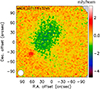 |
Fig. 1 Example of the raw surface brightness image of MACS J0717.5+3745, prior to any filter application (e.g., smoothing), point source removal and deconvolution. The data is dominated by noise on small scales. The cluster diffuse emission is nonetheless visible as a negative decrement, as well as a radio foreground galaxy (positive) on the southeast. The white circle on the bottom left corner provide the NIKA beam FWHM. |
2.3 Algorithms
In order to reveal pressure substructures, we make use of two algorithms, namely a Gaussian gradient magnitude (GGM, see also Roediger et al. 2013; Sanders et al. 2016b) filter and a Difference of Gaussians (DoG, similar to unsharp-masking, as used also in X-ray analysis, see e.g., Fabian et al. 2003) filter. These allow us to identify strong pressure gradients or discontinuities, and pressure peaks at specific scales, respectively.
2.3.1 Gaussian gradient magnitude filter
Because the NIKA data are dominated by noise on small scales, we convolve the maps with a Gaussian kernel,  , of FWHM θ0, to reduce it.We then compute the magnitude of the gradient of the maps as
![Mathematical equation: \begin{equation*} M_{\textrm{GGM}} = \sqrt{\left(\mathcal{D}_{\textrm{RA}} \ast \left[G_{\theta_0} \ast M\right]\right)^2 + \left(\mathcal{D}_{\textrm{Dec}} \ast \left[G_{\theta_0} \ast M\right]\right)^2},\vspace*{-3pt} \end{equation*}](/articles/aa/full_html/2018/06/aa31950-17/aa31950-17-eq6.png) (4)
(4)
where the convolution kernel  along the RA and Dec axis are respectively given by
 (5)
(5)
where Δθ is the map pixel size. The resulting quantity, MGGM, is therefore a measurement of the projected pressure gradient on scale θ0. It is expressed in units of surface brightness per arcmin, and can be converted to physical units of keV/cm3 Mpc per Mpc accounting for the angular diameter distance of the cluster and the conversion coefficients from Compton parameter to Jy beam−1 given in Adam et al. (2017b).
The direction of the gradient is obtained by computing its orientation on the sky, given by the angle
![Mathematical equation: \begin{equation*} \mathrm{\Psi} = \textrm{atan} \left( \frac{\mathcal{D}_{\textrm{Dec}} \ast \left[G_{\theta_0} \ast M\right]}{\mathcal{D}_{\textrm{RA}} \ast \left[G_{\theta_0} \ast M\right]} \right).\end{equation*}](/articles/aa/full_html/2018/06/aa31950-17/aa31950-17-eq9.png) (6)
(6)
2.3.2 Difference of Gaussian filter
In order to extract pressure substructures on a specific scale, we compute the difference of the NIKA maps convolved respectively with Gaussian kernels of FWHM θ1 and θ2:
 (7)
(7)
The filter thus removes signal on scales larger than θ2 and on scales smaller than θ1, allowing us to search for structures in a narrow range of angular scales. The resulting map is homogeneous to the input map, that is, it is sensitive to the projected pressure along the line-of-sight in the selected range of angular scales.
2.3.3 Baseline filtering parameters
The NIKA beam FWHM is 18.2 arcsec at 150 GHz (Catalano et al. 2014). On small scales, the noise dominates over the signal and therefore, the smallest scale at which we can search for substructures is slightly below, but of the order of the beam FWHM, depending on the S/N of the data. As the data reduction attenuates the signal on scales larger than ~ 2 arcmin (see Adam et al. 2015, and Sect. 5), the signal is also dominated by noise on large scales. Consequently the spatial dynamics accessible with NIKA data is about one order of magnitude, between 15 and 150 arcsec (limited by the beam and signal processing, respectively). Here, we aim at detecting pressure discontinuities and compression regions in distant clusters (z > 0.4), which requires probing the smallest scales available. If present, subcomponents are expected to have typical angular size smaller than that of the main clusters (~1–2 arcmin) by a factor of a few. Therefore, we focus on the following baseline parameters for our filters: θ0 = 15 arcsec, and  arcsec. In practice, it is possible to increase the S/N of the filtered maps by increasing the filters scales, at the cost of washing out the signal arising from the substructures we aim to detect. In Appendix A, we show how the extracted signal changes according to the filter parameters.
3 Application to cluster toy models
The filtering algorithms are first tested on toy models in order to highlight the signature of the filtered signal in idealized physical situations. The toy models that we consider are: a spherical generalized Navarro Frenk and White (gNFW) pressure profile (Nagai et al. 2007), a bimodal pre-merging system, a main core plus an extension, and a pressure profile that includes a shock, respectively. We apply the filters using the baseline parameters discussed in Sect. 2.3.3.
3.1 Construction of toy models
The construction of the toy models is described below. The clusters redshift is z = 0.6 because it corresponds to the mean redshift of the NIKA sample (see Sect. 2.2 and Table 1), but we also test other redshifts between z = 0.4 and z = 1.
- 1.
Spherical gNFW profile: one of the most common and simple descriptions of cluster pressure is that of a spherically symmetric radial distribution following a gNFW (Nagai et al. 2007) profile, and before using the filtered maps to investigate disturbances in the ICM, it is important to understand the response of the filters to perfectly spherical cluster signals. We thus simulate such a cluster using the best fit slopes and concentration parameters obtained by Planck Collaboration Int. V 2013 and assuming a characteristic radius R500 = 1000 kpc (comparable to NIKA clusters). The pressure is integrated along the line of sight, to produce an azimuthally symmetric Compton parameter map (Eq. (3)), which we convert into surface brightness in the 150 GHz NIKA band (Eq. (1)). We also use best fit parameter profiles of cool-core and disturbed clusters from Arnaud et al. (2010) to test changes in the steepness of the profile.
- 2.
Bimodal pre-merger system: clusters can form via the merging of sub-clusters and groups. We model such a system using our gNFW model to simulate a pair of identical clusters, separated by 100 arcsec. We add a pressure bar component between the two clusters to mimic the adiabatic compression caused by the merger. The bar has an arbitrary projected size of R500∕5 along the merger direction and R500∕1.5 in the perpendicular direction. The tSZ amplitude of the bar is 0.3 times that of the gNFW components peaks.
- 3.
Main core plus extension: it is common to find clusters made of a main core plus an extension that arises from both post-merger and pre-merger disturbances in the ICM. We model this system by a main gNFW cluster, to which we add a second gNFW sub-cluster with R500 = 300 kpc, normalized to a peak of one third that of the main core, and located 50 arcsec away.
- 4.
Shocks: merging events can cause discontinuities in the ICM gas, such as shocks in the pressure. We thus simulate a radially symmetric cluster including a pressure discontinuity in the profile. We use the Rankine-Hugoniot jump conditions (see e.g., Sarazin 2002, for a review), given by
 , with P1 and P2 the pressure before and after the shock and γad = 5∕3 the adiabatic index. We use a Mach number
  as observed in typical shocks (e.g., Markevitch & Vikhlinin 2007). The pressure profile before and after the jump is described by a power law with index 0 in the inner part (to avoid confusion with the signal that would arise from a steep core, as in the spherical gNFW profile), and index –2 in the outer part, respectively. The pressure is integrated along the line of sight and the resulting Compton parameter profile is used to generate the surface brightness. We consider a shock moving outward, with respect to the cluster center.
The toy model images are finally convolved with the NIKA beam and normalized to have a typical peak surface brightness of –1 mJy beam−1. This corresponds to a Compton parameter of about 10−4 and it is also the typical scale of the NIKA clusters.
3.2 Application of the filters
We first consider the gNFW model (see the maps of Fig. 2, top row). Because the pressure distribution is spherically symmetric, the surface brightness and the filtered maps are azimuthally symmetric (see the profiles of Fig. 3, left panel). The surface brightness profiles are peaked toward the center. We thus observe a ring with a radius that matches the filter plus beam size on the GGM map and profile. This means that at the angular scales recovered by NIKA and the redshift we consider, we are not able to observe a flattening in the profile in the core (if it exists), and the profile surface brightness always appears steeper as we get closer to the center. We observe a ring radius larger than the filter plus beam size, that is, we detect a flattening in the core, only when reaching redshifts lower than 0.5, in the case of the disturbed clusters pressure profile (i.e., the flattest that we consider here Arnaud et al. 2010). On larger scales, the GGM map smoothly vanishes. The null of the GGM map coincides with the cluster center due to smoothing. The typical scale of the gradient peak is 0.8–1.2 mJy beam−1 arcmin−1, for a surface brightness normalized to –1 mJy beam−1 at the maximum decrement. The DoG maps allow us to extract the core signal, whose amplitude is typically 20–30% of that of the peak at our scales.
The middle row of Fig. 2 provides the maps of the bimodal cluster. The GGM map is elongated along the merger axis.The strong gradients on the north and south are due to the bar, that produces an artificial edge on the surface brightness (before filter and beam smoothing), and we also observe the gradient resulting from the gNFW cores on the east and west sides. The DoG map allows us to clearly define the different components that would not necessarily be obvious on the surface brightness map in particular in the presence of noise (see also Sect. 5).
The case of the main core plus extension is given on the bottom row of Fig. 2. The GGM map presents two minima thatcorrespond to the two cores and the gradient is reduced between the two sub-clusters, with respect to the single gNFW profile. Similarly to the bimodal case, the DoG map allows us to clearly identify the two components and their locations.
Figure 3 (right panel) presents the toy model and the corresponding filter response as a function of radius, in the case of the shock, similarly to the signal that one would extract along cones in the direction of the shock. It provides the pressure profile (P, as a function of the physical radius, r, in 3D), the surface brightness profile (as a function of the projected radius R, in 2D), and the filtered map profiles, GGM(R) and DoG (R), respectively. The shock location is rshock = 400 kpc. Because of line of sight integration, the surface brightness profile does not present a trivial discontinuity. Instead, it progressively vanishes before the shock. The sharp discontinuities and peaks are then degraded due to instrumental beam smoothing. The GGM filter allows us to pick up the strong gradients in the map, and is thus well designed for highlighting shocks. It presents a peak associated to the shock, but it is not coincident with it (due to smoothing). The DoG filtered maps allow us to highlight compact substructures and the filter is efficient to pick up the cluster core. For such a shock and filter parameters, the GGM amplitude typically reaches 1–2 mJy beam−1 arcmin−1, depending on the distance from the center via the amplitude of the surface brightness at the shock location. The DoG amplitude reaches –0.1–0.5 mJy beam−1.
The different toy models show the expected signal after application of the filters under simplistic assumptions, but they correspond to typical features that one can expect in the NIKA sample. It is clear that the filtered maps provide a new way to look at our data, in particular in terms of morphological studies. At the angular scales probed by NIKA and the redshifts we consider (i.e., that of the NIKA sample), we can however see some limitations when pushing the extraction of the features to smaller angular scales. As a typical example, Fig. 3 (right panel) shows that a shock will be hardly distinguishable from a ramp at redshifts above 0.5. Similarly, the cluster core, even if purely spherical, will also show up at amplitudes similar to that of the signal arising from merging events that we want to extract.
The most accessible features correspond to scales of a few tens of arcsec, that is a few hundred kpc. Following this preparatory exercise on toy models, below we test the performances of the filters under controlled but realistic situations using cosmological hydrodynamic simulations.
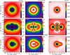 |
Fig. 2 Surface brightness and GGM and DoG response to the tSZ signal expected for a spherically symmetric gNFW pressure profile (top), a bimodal cluster plus a pressure bar (middle), and a main core plus an extension (bottom). Left: tSZ simulated surface brightness. The white circle on the bottom left provides the beam FWHM. Middle: GGM filtered maps with θ0 = 15′′. The white vectors represent the direction of the gradient, Ψ. Right: DoG filtered maps with θ1 = 15′′ and θ2 = 45′′. |
4 Application to hydrodynamical simulations
Before performing our analysis on the NIKA data, we test the behavior of the filters described in Sect. 2 by using realistic simulated cluster data. Such simulations also aid in the interpretation of the observed structures in real data, in addition to the toy models described in Sect. 3. To do so, we use synthetic tSZ images extracted from the RHAPSODY-G simulations for different cluster configurations.
4.1 Extraction of tSZ maps from the RHAPSODY-G simulations
The RHAPSODY-G simulations (Wu et al. 2013; Hahn et al. 2017) is a suite of cosmological hydrodynamics adaptive mesh refinement zoom simulations of ten massive clusters. The simulations include cooling and sub-resolution models for star formation and supermassive black hole feedback.
Boxes of co-moving volume  were used to extract Compton parameter maps around the clusters by integrating Eq. (3) along a fixed line-of-sight direction using the gas pressure in each grid cell. These maps were converted into surface brightness images in the NIKA 150 GHz bandpasses (see the coefficient provided in Adam et al. 2017b). We neglect relativistic corrections, as they can only reduce the surface brightness by up to 8% for the hottest clusters at our frequency (Itoh & Nozawa 2003). The maps were produced for a large subset of the available simulation snapshots (about 150 per cluster), tracing the evolution of the clusters from redshift z ~ 1.5 to z = 0. The knowledge of the cluster formation history from the simulation data is a key point for the interpretation of the maps.
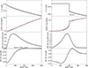 |
Fig. 3 Left: GGM and DoG response to a gNFW radial pressure profile. The vertical dashed line provides the physical size corresponding to the 15 arcsec filter plus the NIKA beam size, at the cluster redshift. Right: GGM and DoG response to a shock propagating outward, in a radially symmetrical way, with Mach number
|

4.2 Selection of a RHAPSODY-G sub-sample
A sub-sample of clusters was selected to assess the substructure detection in a quantitative way and to investigate the behavior of the filters in detail (see Sect. 5 for the end-to-end processing of the simulations). The clusterswere selected to match the redshift range of the NIKA sample (see Sect. 2.2) and to explore various cluster configurations. We thus restricted the RHAPSODY-G snapshots to the redshift range 0.4 ≲ z ≲ 1 and selected five distinct snapshots (see Fig. 4), by visual inspection, for different clusters1:
- 1.
RG361_00188: a relaxed spherical cluster at redshift z = 0.61, with minimal merging activity since z ≳ 1. The cluster is slightly elongated along the line-of-sight.
- 2.
RG474_00172: a major merger at z = 0.90. The two main sub-clusters already passed through each other, the closest encounter happening at z ~0.95. The merger axis is close to the plane of the sky.
- 3.
RG377_00181: a triple-merger with two objects of almost equal mass and a smaller sub-group at z = 0.54. The two main sub-clusters have already experienced a first encounter at z ~ 0.59, while the smaller group is spatially coincident (aligned) with one of the two main clusters.
- 4.
RG448_00211: a relaxed, slightly elliptical cluster, exhibiting strong active galactic nuclei (AGN) feedback at z = 0.40, which produces a pressure shell around the main core.
- 5.
RG474_00235: a very massive cluster, corresponding to the evolved version of RG474_00172, at z = 0.39. This cluster was selected mainly because it is relatively nearby and very massive, such that its spatial extent fits better that of the NIKA clusters, allowing us to validate our procedure in such cases. It is undergoing a major merger, mostly oriented along the line-of-sight.
We note that the RHAPSODY-G cluster masses match well those of the NIKA sample at redshift zero, but they are lower by a factor of a few at the considered redshifts (except for RG474_00235, which reaches a mass similar to the most massive NIKA cluster). Therefore the simulated surface brightnesses are also lower by a factor of ~ 2. A summary of the main properties of the four RHAPSODY-G selected clusters is provided in Table 2.
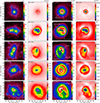 |
Fig. 4 Application of the filtering algorithms to clusters from the RHAPSODY-G suite of simulations. From top to bottom, the clusters are RG361_00188, RG474_00172, RG377_00181, RG448_00211, and RG474_00235 (see also Table 2 for the main properties of the sample). Left: projected dark matter density. Contours are linearly spaced. Units are arbitrary. Middle left: input raw tSZ surface brightness maps with dark matter map contours overlaid. Units are mJy beam−1. Middle right: GGM filtered maps with θ0 = 15′′. The white vectors represent the direction of the gradient, Ψ. Units are mJy beam−1 arcmin−1. Right: DoG filtered maps with θ1 = 15′′ and θ2 = 45′′. Units are mJy beam−1. The contours provide the true S/N expected for the simulation of the observation of these sources done in Sect. 5. They are given by steps of 2σ excluding 0 (see Sect. 5 for further discussions about the S/N estimates). |
Summary of the properties of the RHAPSODY-G selected cluster sample.
4.3 Filter application to raw RHAPSODY-G tSZ images
We first apply the filters defined in Sect. 2 to the raw RHAPSODY-G surface brightness images (i.e., without including noise or observational artifacts). The filtering parameters are set according to our baseline choice (Sect. 2.3.3), as optimized for the NIKA sample. Figure 4 provides images of the input surface brightness of the RHAPSODY-G selected sample, and the corresponding filtered maps together with the projected dark matter density distribution.
RG361_00188 (relaxed) presents a very compact core and is azimuthally symmetric. The tSZ signal matches well that of the dark matter. As the steepness of the surface brightness profile increases toward the center, the corresponding GGM map is null at the cluster peak and exhibits a quasi perfect ring with radius matching the filter scale (see also the gNFW model of Fig. 2), with a small excess in the south. The DoG map presents a single compact core component. The RG474_00172 and RG377_00181 (major and multiple mergers, respectively) tSZ maps show that the two clusters are both clearly non-spherical. The corresponding dark matter maps reflect the presence of multiple sub-clusters and the dark matter distribution deviates significantly from that of the tSZ signal. The GGM maps provide additional information by highlighting regions of strong gas compression. In the case of the major merger, RG474_00172, we observe a strongly elongated ring with two main pressure gradients in the east and west regions, comparable to the merger toy model of Fig. 2 without the bar component. Discontinuities are observed in the simulation at these locations, but they are too close to the core to be distinguished from it considering our baseline scales, and the signal we observe results from the sum of the shocks and the gNFW-like steep cores, as an overall compression. In the case of the multiple merger, RG377_00181, a strong gradient is visible in the west region, corresponding to the main core, and a ~ 70 arcsec (460 kpc) long arc propagates through the ICM on the southeast sector, corresponding to another sub-cluster moving within the ICM of the main cluster and causing a shock. The DoG maps present a double peak structure, allowing us to quantitatively identify the two sub-clusters in the case of RG474_00172. In contrast, one only finds a main core plus a weak extension in the case of RG377_00181 (comparable to the main core plus extension toy model of Fig. 2). In agreement with the dark matter distribution, RG448_00211 appears to be relatively relaxed and azimuthally symmetric. However, the GGM map reveals, in addition to the steep core, the presence of a pressure shell responsible for a strong gradient ring extending 45 arcsec (250 kpc) away from the peak. This is due to the feedback from the central AGN onto the ICM, and possibly an artifact of the specific implementation of AGN feedback as a thermal blastwave in these simulations. We also observe a plateau extending to 45 arcsec (250 kpc) radius on the DoG filtered map and we note that the core signal is slightly elongated with a main axis inclined by about 20 degrees with respect to the RA axis. RG448_00211 presents a structure that compares well to RG377_00181, both in the dark matter and the gas distribution. However, no shock front can clearly be identify, probably due to projection effects since the merger axis is mainly along the line of sight in this case. In addition, both the amplitude and the angular size of RG448_00211 are much larger than RG377_00181, because it is located at lower redshift, and because its mass is about 3.5 times larger. RG448_00211 is mainly used to validate our analysis, even in the case of very bright and very extended clusters (see Appendix B).
The morphologies seen in the filtered RHAPSODY-G sub-sample provide templates that we can compare to the structures observed in the real NIKA data. In practice, we performed this analysis using all available RHAPSODY-G snapshots and projected the data along three line-of-sight directions. Therefore, we dispose of a much larger variety of configurations, even if the four selected clusters already qualitatively sample most of the structures visible in the simulation, according to the selection of the sub-sample. These templates will allow us to better understand the physics at play in the NIKA clusters, in particular in merging systems. When using the tSZ signal as a tracer of the overall matter distribution (e.g., Adam et al. 2015, 2016; Ruppin et al. 2017), the application of such filters could also help to interpret scatters and biases between the total mass distribution and the tSZ signal, as such features reflect spatial misalignment between the dark matter distribution and the hot gas.
In summary, the GGM and the DoG filters allow for the detection of strong gradient in the surface brightness (seen as ridges in the GGM maps), and tSZ peaks in the RHAPSODY-G images, respectively. They provide templates for interpreting features observed in the NIKA data in Sect. 6. These features correspond to shocks and gas compressionregions induced by merging events, and the main cores of the merging sub-clusters, respectively. In the case of isolated spherical clusters, GGM features are also observed, showing up as rings around the tSZ peak.
5 Systematic effects and noise properties
In addition to the tSZ substructures, NIKA data are affected by several systematic effects that can potentially alter the reconstructed filtered images. In this Section we test the response of the filters described in Sect. 2 to potential bouncing artifacts due to the transfer function of the NIKA processing, spatially correlated noise, and point source residuals.
5.1 NIKA processing of the RHAPSODY-G sub-sample
While the DoG filter is linear and preserves the Gaussian nature of the noise, this is not the case for the GGM filter. Therefore, in order to validate the behavior of the filter, we use end-to-end realistic simulations of the observations and post-processing of the RHAPSODY-G sub-sample, including all the artifacts present in the real data, but for which the true input signal is known.
To obtain simulated observed surface brightness images, we make use of the real raw telescope time ordered data (TOD) collected for the cluster MACS J0717.5+3745 (the one with the largest observing time, see Sect. 6), in which we inject the signal corresponding to the considered RHAPSODY-G tSZ maps, according to the telescope scanning strategy. Prior to adding the simulated signal to the data, half of the TOD scans are multiplied by − 1 in order to cancel the astrophysical signal present in the real data, on the final co-added map. We aim at obtaining simulations corresponding to the highest S/N NIKA clusters. Therefore, before adding the simulated signal to the TOD, the noise is rescaled by the ratio of the RHAPSODY-G clusters peak surface brightness to the one of the deconvolved map of MACS J0717.5+3745 (typically a factor of ~ 2, see Sect. 4.2). We note that this high S/N case also allows us to check the behavior of the filters in the low S/N regime. Indeed, the S/N is maximal at the peak, but smoothly vanishes towards the outskirts. Nevertheless, we also consider the case where the S/N peak is 4, at 22 arcsec resolution (lowest S/N NIKA cluster, PSZ1 G046.13+30.75), to validate our procedure in the cluster center in this regime (Appendix B). After including the simulated signal, the TOD are then processed similarly to the one of the real NIKA clusters (see Adam et al. 2015, for more details).
Finally, we obtain realistic maps of the RHAPSODY-G sub-sample, as if they were truly observed using NIKA, with a S/N peak of about 20, at 22 arcsec resolution. The maps, once deconvolved from the processing transfer function (see Sect. 5.2), are displayed in Fig. 5, together with their GGM- and DoG-filtered maps obtained using our baseline parameter values (cf. Sect. 2.3.3). These maps can be compared to that of Fig. 4 to validate our procedure, and they are used in the following Subsections to quantify the properties of the filtered maps in the presence of systematic effects and noise.
5.2 Transfer function filtering
By construction, the zero level surface brightness of the NIKA maps is not defined. However, this does not affect the results presented inthis paper since both the GGM- and DoG-filtering procedures are insensitive to zero-level effects. In addition, the NIKA processing transfer function reduces the signal on scales that are larger than the instrument field of view (~ 2 arcmin). After deconvolution, small differences can remain between the deconvolved image and the original input image, due in particular to anisotropies in the scanning strategy and uncertainties in the estimated transfer function. However, these differences are mostly prominent on scales larger than the NIKA field of view, where filtering effects are important (Adam et al. 2015). By comparing the NIKA-like processed RHAPSODY-G sub-sample to the non-processed maps, we find that these differences have a negligible impact on the filter application with respect to the noise (see also Figs. 4 and 5). In Appendix B, we provide more details on the deconvolution and its impact on the results.
5.3 Noise spatial correlations and propagation through the filters
The NIKA noise is Gaussian and spatially correlated (Adam et al. 2016) but its behavior does not necessarily propagate in a trivial way under the application of the filters, especially in the case of the GGM filter, which is non-linear. In order to estimate the significance of the structures that we observe in Sect. 6, we use noise realizations of the surface brightness maps generated as described in Adam et al. (2016). They account for the map pixel-to-pixel correlated noise induced by residual atmospheric and electronic noise, the inhomogeneities of the noise due to the scanning strategy, and the contribution of the cosmic infrared background, which is non-negligible for the deepest observations. For each cluster, we produce a set of 1000 surface brightness noise realizations, N(i), which are deconvolved from the transfer function associated to the NIKA data processing similarly to their corresponding cluster data and used to estimate the noise in the filtered maps using the following procedure.
As the DoG filter is linear and preserves the noise Gaussianity, we process these surface-brightness-noise-only Monte Carlo realizations through the same filter as the data. Then, we estimate the respective DoG filtered maps standard deviation by taking the root-mean-square of all the processed Monte Carlo realizations, for each pixel of the map. The DoG S/Ns are straightforwardly obtained by normalizing the filtered cluster data by the standard deviation maps, and follow Gaussian statistics.
According to the definition of Eq (4), the noise of the GGM filtered maps depends on the surface brightness signal itself because of the non-linearity of the filter. Therefore, we use the observed signal as an estimate of the true signal, Ŝ, to which weadd the surface brightness noise realizations, prior to processing them through the GGM filter.The estimate of the filtered map noise contribution, from each Monte Carlo realization i, is then given by
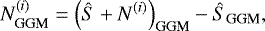 (8)
(8)
where the index GGM corresponds to the filter application defined by Eq (4). For each pixel of the map, we compute μGGM and σGGM, the mean and the standard deviation of the noise realizations  per map pixel, respectively. Accounting for the non-zero mean of the filtered map noise, the effective S/N is defined as
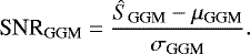 (9)
(9)
In practice, the estimated surface brightness signal is the sum of the true signal, S, and the noise, N, as Ŝ = S + N. In the low surface brightness S/N regions, Ŝ is therefore dominated by the noise, which can mean that our estimations are biassed toward lower values of μGGM. In the case of the RHAPSODY-G sub-sample, we also dispose of the true input surface brightness signal, Ŝ = S, and we use it to compute the true S/N, to quantify the reliability of our S/N estimation procedure, as discussed below.
The noise distribution is illustrated in Fig. 6 for both the GGM and the DoG filters. The data of CL J1226.9+3332 are used as an example, in the case of our baseline filter parameters (Sect. 2.3.3). The histograms account for the pixels that are enclosed within 30 arcsec from the cluster center, where the noise is homogeneous. In the case of the GGM filter, we consider both the possibility in which the cluster signal, Ŝ, is set to the measured signal from CL J1226.9+3332, and where it is set to zero in Eq. (8), to illustrate the noise behavior in low S/N regions. As we can see, the DoG noise statistics (Fig. 6, left panel) is described by a Gaussian distribution with a mean compatible with zero, by construction. The GGM noise distribution is well described by a Gaussian distribution in signal-dominated regions (middle panel). However, as the signal vanishes, such as in the external regions, the noise becomes non Gaussian, its mean increases and the distribution becomes positively skewed. Despite the fact that the non-zero mean of the noise is corrected for when computing the significance of the data, we note that the noise is boosted by up to 15% (in the wing of the distribution) in the extreme case of zero signal, with respect to what one would expect for Gaussian noise (Fig. 6, red line).
The validation of the S/N reconstruction of the GGM filtered maps is illustrated in Fig. 7. It shows the estimated S/N as a function of the true S/N, computed using the RHAPSODY-G sub-sample for which both Ŝ and S are available. We can observe that in the low S/N regime, the estimated S/N is overall biased high, due to the fact that μGGM is biased low. At higher S/N (≳3), the estimated S/N converges to the true S/N within a few percent. Our procedure is thus valid in this regime.
Finally, we use the end-to-end processed and filtered maps from a RHAPSODY-G sub-sample, shown in Fig. 5, to check that the structures we recover are reliable. Indeed, above three, the S/N of the recovered features is consistent with what we expect in the case of the raw maps of Fig. 4 when using the true S/N.
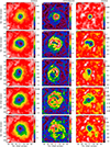 |
Fig. 5 As in Fig. 4 but for the case of end-to-end processing of the simulated RHAPSODY-G sub-sample: surface brightness maps (left), GGM filtered maps (middle) and DoG filtered maps (right). From top to bottom, the clusters areRG361_00188, RG474_00172, RG377_00181 and RG448_00211 (see also Table 2 for the main properties of the sample). The surface brightness images are deconvolved from the transfer function (but not from the beam smoothing) and the S/N contours are estimated as in the case of real data (separated by steps of 2σ). |
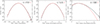 |
Fig. 6 Noise distribution of all the pixels enclosed within 30 arcsec radius from the cluster center, in the case of CL J1226.9+3332, for our baseline filter parameters. The red curves provide the best Gaussian fit to the histograms. Left: DoG noise histogram. Middle: GGM noise histogram in the case of Ŝ set to the observed signal of CL J1226.9+3332. Right: GGM noise histogram in the case where Ŝ = 0 in Eq (8). |
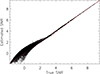 |
Fig. 7 Comparison of the estimated GGM filtered maps S/N as a function of the true S/N, using the RHAPSODY-G sub-sample. The estimated S/N is computed using the NIKA processed RHAPSODY-G sub-sample (Eq. (9)). The red dashed line represent the one to one correspondence. Each point corresponds to a pixel of the map. |
5.4 Point-source residuals
Foreground, background, or cluster-member galaxies can show up as point sources in tSZ images, which constitutes a well known potential bias. In the case of NIKA, these sources are subtracted either by fitting their flux together with the tSZ signal (Adam et al. 2015), or by modeling their spectral energy distribution (SED) and fitting them to multi-wavelength photometric data to extrapolate their flux in the respective NIKA bands (see the method detailed in Adam et al. 2016). Even if such procedures provide a good first estimate of the contaminant, they are limited by the accuracy of the model to describe the data, the limited available extra data, and miscentering arising from limited accuracy in the source coordinate or telescope pointing precision. At 150 GHz, the contaminant sources are mostly radio galaxies, but infrared galaxies can also have a significant contribution.
We estimate the impact of residual point sources by considering the following approach in two upper limit cases:
- 1.
Point sources below the detection threshold that are not subtracted: we simulate point sources with a flux of 3σ times that of the noise rms, and assume that it is not subtracted from the tSZ map.
- 2.
Point sources that are poorly subtracted: we assume a given degree of contamination by simulating a 3 mJy point source (the typical flux of the brightest radio sources observed in the NIKA clusters at 150 GHz), which we subtract assuming a flux that is off by 10%, and including a miscentering offset of 3 arcsec (the NIKA pointing accuracy for one scan Catalano et al. 2014).
As the GGM filter is not linear, the point source contamination induced by the application of the filter depends not only on the point sources themselves, but also on the local environment of the source. Therefore, we test both the case where the sources are simulated in the outskirts of the clusters, where the noise dominates, and within a few arcsec of the cluster core, where the signal dominates.
Using our baseline filter parameters, we find that the difference between the point-source-contaminated and the tSZ-only maps can reach deviations of up to 4σ, both for the GGM and the DoG filters. As the S/N of the simulated clusters is set to match the highest-S/N NIKA clusters, it represents an upper limit of the contamination. In addition, the biases remain local on the maps and exhibit specific structures that are distinct from the ones that appear in the case of interacting clusters (ring-like shaped, azimuthally symmetric, or dipole-like at the scale of the filter, see Fig. 4). Nonetheless, point source residuals could mimic compact tSZ cores, at the scale of the beam. As we increase the filter scales, the signal arising from point source residuals quickly becomes insignificant. The signatures of point source residuals are illustrated in Fig. 8. Due to the non-linearity of the GGM, the corresponding extra signal arising from point sources can slightly deviate from the one shown in Fig. 8.
We conclude that undetected or mismodeled point sources are an unavoidable potential bias. They can affect the interpretation of the signal at the level of a few σ, but they cannot lead to a mis-interpretation of the overall signal observed in tSZ maps as the contamination remains local. Other artifacts areexpected to produce negligible signal in our filter data. Despite the nonlinearity of the GGM filter, we have developed a method to estimate the statistical significance of the corresponding signal that is accurate above a S/N of three.
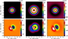 |
Fig. 8 Application of the filters to point source residuals in case 1 (no source subtraction, top) and case 2 (source improperly subtracted, bottom). The input point source flux has been normalized to one. Left: input surface brightness map. Middle: GGM filtered map. Right: DoG filtered map. |
Coordinates of the main X-ray peak.
6 Application to the NIKA clusters sample
The NIKA surface brightness maps at 150 GHz are provided in Fig. 9 together with the filter algorithm results. They are deconvolved from the processing transfer function, smoothed to an effective resolution of 22 arcsec FWHM and cleaned from point source contamination. The three clusters, RX J1347.5–1145, MACS J1423.8+2404, and PSZ1 G046.13+30.75, have been imaged with NIKA. Despite the relatively low significance of this sub-sample (less than 10σ per beam at the22 arcsec resolution), we apply the GGM and DoG filter to the maps. We observe hints for internal structures, but only at low significance level, as briefly discussed below. The three other NIKA clusters, MACS J0717.5+3745, PSZ1 G045.85+57.71, and CL J1226.9+3332, present a peak significance greater than 10 σ at the 22 arcsec resolution, with a maximum of more than 18σ for MACS J0717.5+3745 (see Fig. 9). This is comparable to the RHAPSODY-G processed tSZ maps of Fig. 5 and we thus expect to be able to find substructure features at a similar significance within these clusters. The GGM- and DoG-filtered maps of the NIKA clusters are presented in Fig. 9 for our baseline filter parameters. In the following Subsections, we discuss the individual cluster analyses.
6.1 RX J1347.5–1145
RX J1347.5–1145 is a massive cluster at redshift 0.45, and one of the most luminous X-ray clusters. Being an extremely bright tSZ source, it has already been observed using the tSZ effect by several groups (e.g., Komatsu et al. 1999; Pointecouteau et al. 1999; Kitayama et al. 2004, 2016; Mason et al. 2010; Plagge et al. 2013; Adam et al. 2014; Sayers et al. 2016). RX J1347.5–1145 presents a dense core, but also shows an extension toward the southeast, which is associated with the merging of a sub-cluster. The tSZ peak is aligned with the southeast extension, corresponding to the overpressure caused by the merger in this region. This cluster was observed with an early setup of the NIKA instrument (bandpass, sensitivity, calibration procedure; see Adam et al. 2014, for more details). In addition, the scanning strategy was not isotropic due to a mistake in the control software, leading to possible uncontrolled systematics in the filtered map. Therefore, the application of the filtering algorithms on the NIKA map of RX J1347.5–1145 is meant to remain qualitative in this paper. The GGM-filtered map presents a ≳ 2σ ridge (≳ 4σ when using θ0 = 20 arcsec) inclined by 40 degrees with respect to the Dec axis, about 30 arcsec (178 kpc) east from the X-ray center. It could be associated to the eastern shock front seen in Chandra data by Kreisch et al. (2016), but deeper tSZ observations are necessary to confirm this. The DoG-filtered map shows that the tSZ pressure in the cluster core is elongated from SE to NW. Large scales being filtered out, the morphology of the map compares well with that of MUSTANG (Mason et al. 2010) and ALMA (Kitayama et al. 2016), which are sensitive to smaller scales and intrinsically filter out large scales. The tSZ SE extension that we observe, and which is tracking a hot spot in RX J1347.5–1145, is coincident with that identified by NOBA (Nobeyama Bolometer Array Kitayama et al. 2004) and DIABOLO (on the IRAM 30 m telescope Pointecouteau et al. 1999, 2001) observations. Nevertheless, the exact location of the tSZ peak is not clear due to the uncertainties in the flux of a radio source located in the brightest cluster galaxy.
6.2 MACS J1423.8+2404
MACS J1423.8+2404 is a very relaxed system and a typical cool-core, at redshift 0.55. The corresponding NIKA observations and data reduction are detailed in Adam et al. (2016), including a detailed description of the cluster. The peak S/N of the NIKA map reaches about 6 at the 22 arcsec resolution. The GGM and DoG maps do not allow us to identify substructures that deviate from that expected for a spherically symmetric object, within the noise fluctuations whose magnitude is large. A small GGM excess (≳ 4σ), with respect to gNFW expectation (see Fig. 2), is visible in the south, but point source contamination (AGN and IR) is strong near the cluster center, and this could be due to mis-modeling of the contamination (see Adam et al. 2016, and the discussion of Sect. 5.4).
6.3 MACS J0717.5+3745
MACS J0717.5+3745 is one of the most disturbed clusters known to date. It is made of at least four interacting sub-clusters (Ma et al. 2009), and is thus an excellent target to search for compression regions, discontinuities, and secondary peaks in tSZ maps. In addition to the systematic uncertainties discussed in Sect. 5, MACS J0717.5+3745 contains a significant amount of kinetic Sunyaev-Zel’dovich (kSZ; Sunyaev & Zeldovich 1980). Because of large uncertainties in the estimates of this contaminant, it is only possible to test the impact of the kSZ signal on our result by comparing the recovered signal in the cases with and without kSZ correction, as detailed in Appendix C. Since MACS J0717.5+3745 disposes of excellent X-ray data, we also provide a multi-wavelength view of the cluster together with our filtered maps in Fig. 10.
The disturbed dynamical state of MACS J0717.5+3745 is obvious, as can be observed in Figs. 9 and 10. The overall structure of the GGM and the DoG maps are the same for the case with and without kSZ, but the relative amplitude of the structures strongly depends on the correction (see Appendix C). Therefore, the kSZ contaminant only allows us a qualitative estimate of the gas inner structure. The GGM maps present two strong ridges on the east and southeast regions, of ~ 1 arcmin (395 kpc) each (SNRGGM > 8). In addition, we observe a large arc (~90 arcsec) in the west sector that surrounds the X-ray main core. The southeast GGM ridge is spatially coincident with the southeast edge of the hot temperature bar caused by adiabatic compression (see Fig. 10), and could trace a shock in this region (see also thecomparison to X-ray in Fig. 11, and the corresponding discussion below). The eastern GGM ridge is nearly aligned with a radio relic (see, e.g., van Weeren et al. 2017), and both could be sourced by a shock caused by the ongoing merger. It also corresponds to a secondary vertical structure in the temperature map. The null of the gradient (i.e., flat surface brightness or constant projected ICM pressure) extends across all the brightest regions of the cluster in the case without kSZ correction, while it presents two nulls for the kSZ cleaned version of the map. In both cases, the main X-ray peak is aligned with a null region of the gradient, but we note that the the X-ray structure is itself complex and presents several peaks. Both DoG maps highlight the presence of two main peaks in the pressure distribution (at > 4σ). This was also observed by Mroczkowski et al. (2012) using MUSTANG data. One of the peaks coincides with the main X-ray peak while the other one is coincident with the most massive sub-cluster, as identified from a strong lensing reconstruction (e.g., Limousin et al. 2016). It is also the location of the hottest region that shows adiabatically compressed gas from the merger of the two main clusters. Weaker extensions in the DoG map, such as the one extending to the southwest, coincide with secondary X-ray peaks and allow us to identify substructures also in the pressure distribution.
In Fig. 11, we focus on the southeast ridge (the brightest one) by providing the surface brightness and GGM profiles in a slice of the cluster that encloses the ridge (see the gray dashed line in Fig. 9). We also compare these profiles to the X-ray photon count, as measured using Chandra data. We can see that the most prominent GGM feature traces well the steepest surface brightness change in the profile, which is possibly related to a discontinuity in the pressure. It also corresponds to a jump in the density, as probed by the X-ray photon counts, which is expected in the case of a shock. We note that the latter is offset by about 7 arcsec with respect to the GGM expectation. However, this could be the result of the very different resolution of Chandra and NIKA, 0.5 and 18.2 arcsec, respectively, or projection effect in such a complex system.
The GGM- and DoG-filtered maps of MACS J0717.5+3745 compare well to multiple major mergers as identified in the RHAPSODY-G simulation. They provide further insight into the gas structure of the cluster, with respect to the surface brightness image, by allowing us to identify regions of compressed gas. They are consistent with a major merger of two main sub-clusters and that of one (or more), likely smaller, additional sub-cluster. Nevertheless, projection effects limit our interpretation of the data, in particular in the case of such a complex object. Using the filtered maps together with multi-wavelength data might in the future provide a better understanding of the ongoing merger scenario.
MACS J0717.5+3745 is among the most violent mergers in the Universe, in which kSZ contamination is expected to be large (Mroczkowski et al. 2012; Sayers et al. 2013; Adam et al. 2017b), and where the gas can reach a temperature of up to 25 keV (e.g., Adam et al. 2017a). As shown in Appendix C, kSZ contamination can significantly alter the relative brightness and location of the tSZ peaks we identify using the DoG filter. Similarly. the location of the identified ridges in the GGM map can change significantly when considering the kSZ signal. While MACS J0717.5+3745 is certainly an extreme case (the only single cluster in which kSZ has been clearly detected so far), we note that the kSZ signal potentially affects all the tSZ maps to some extent, and thus the filtered maps. Unfortunately, the current sensitivity to kSZ imaging is not yet sufficient to extract accurate kSZ corrections for all clusters in our sample. By using maps of the ICM temperature (e.g., Adam et al. 2017a), it is possible to account for relativistic corrections to the tSZ spectrum in the NIKA band. In the hottest region of the cluster (~ 25 keV), the correction reaches 13% (see also Table 1 in Adam et al. 2017b), and the relative amplitude of the correction is 8% over thecluster extension. By comparing the filtered map with and without considering the correction, we find that only the amplitude of the signal can change significantly (by typically 10%), but the relative spatial variations are not significant with respect to the noise. Since MACS J0717.5+3745 is the most disturbed and the hottest cluster in our sample, it is thus justified to neglect relativistic corrections for our purpose. Accounting for them would require high-resolution mapping of the temperature, which is generally difficult to achieve at high redshift.
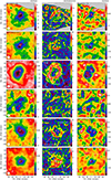 |
Fig. 9 Redshift-ordered maps of the NIKA cluster sample at 150 GHz. Left: surface brightness images. Each map has been smoothed to an effective angular resolution of 22 arcsec FWHM, as shown by the bottom left white circle. Point sources have been subtracted and the data have been deconvolved from the transfer function, but the zero level absolute brightness remains unconstrained. Middle: GGM filtered maps. Right: DoG filtered maps. In all cases, contours provide the S/N, starting at ± 2σ and increasing by 2σ steps. The white crosses provide the main X-ray peak (see Table 3). In the case of MACS J0717.5+3745, the kSZ contribution is not accounted for in the map presented here (see Appendix C and Sect. 6.3 for more details). In the case of CL J1226.9+3332 and MACS J0717.5+3745, the dashed lines correspond to the cone used to define the GGM ridge region when extracting profiles in Figs. 12 and 11. |
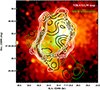 |
Fig. 10 Multi-probe view of the cluster MACS J0717.5+3745: Chandra X-ray surface brightness image (ObsID4200), plotted on a square root scale (thus proportional to the projected density) with XMM-Newton temperature (green contours from Adam et al. 2017a) and the DoG (black contours) and GGM (white contours) maps overlaid. |
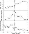 |
Fig. 11 Profile of MACS J0717.5+3745 in the region defined to include the strongest GGM ridge (east ridge, see Fig. 9, as the dark gray dashed line on the surface brightness image). The dashed-dotted line correspond to the GGM ridge location. Top: surface brightness profile. Middle: GGM profile. Bottom: Chandra photon count per unit area profile. |
6.4 PSZ1 G046.13+30.75
PSZ1 G046.13+30.75 is a Planck-discovered cluster (Planck Collaboration XXIX 2014), at redshift 0.55, and was observed during the same campaign as another NIKA cluster, PSZ1 G045.85+57.71 (see Ruppin et al. 2017, for more details). The observing weather conditions were unstable with a high opacity and the cluster significance barely reaches 4σ per 22 arcsec FWHM beam at the peak on the NIKA map. The GGM- and DoG-filtered maps are consistent with noise.
6.5 PSZ1 G045.85+57.71
PSZ1 G045.85+57.71 is a Planck-discovered cluster (Planck Collaboration XXIX 2014), at redshift 0.61, and was observed during the same campaign as PSZ1 G046.13+30.75 (see Ruppin et al. 2017, for more details). It was classified as a cool-core cluster based on its temperature and entropy profile, both fully consistent with the REXCESS cool-core sub-sample (Böhringer et al. 2007; Arnaud et al. 2010; Pratt et al. 2010). Its morphology is highly elliptical, with a main axis oriented about 45 degrees with respect to the RA axis, as can be observed in Fig. 9, but Ruppin et al. (2017) do not find evidence for merging activity. The tSZ peak is consistent with that of the X-ray, and the tSZ elongation is mostly prominent toward the southwest.
The GGM map of PSZ1 G045.85+57.71 is that of an elongated ring following the morphology of the cluster. On the southeast region, we observe a stronger pressure gradient extending over about 45 arcsec (312 kpc) and reaching SNRGGM = 5.8. In contrast to the RHAPSODY-G relaxed cluster RG361_00188, the GGM map shows that the projected pressure is approximately constant (i.e., null of the gradient, or constant surface brightness), over a wide area from the X-ray core to the southwest extension. PSZ1 G045.85+57.71 is a cool-core cluster with a dense X-ray core, indicating that the temperature rises in the southwest sector. The DoG map does not show the presence of any strong core and is consistent with the projected pressure being relatively constant from the X-ray core to the southwest extension. As a consequence of the lack of signal on small scales, the DoG map significance is relatively low, reaching only 4σ at the peak. The main peak is located within a few arcsec of the X-ray core, but two secondary peaks are visible toward the southwest and to the north.
The GGM and DoG images of PSZ1 G045.85+57.71 are consistent with that of a merging sub-group falling from the southwest to the main cluster. This sub-group could be responsible for the local temperature rise and the gas overpressure in the southwest. Such scenarios are commonly observed in the RHAPSODY-G clusters. In contrast, relaxed RHAPSODY-G systems do not present similar features in their filtered maps, which reinforces the interpretation proposed above. Nevertheless, we note that the S/N remains limited in the case of this cluster, and any stronger conclusions would require deeper data.
6.6 CL J1226.9+3332
CL J1226.9+3332 is a hot and massive high redshift cluster, at z = 0.89. It was discovered by ROSAT (Ebeling et al. 2001) and has been the subject of several multi-wavelength studies since then. In particular, Maughan et al. (2007) identified a temperature excess in the southwest region from XMM-Newton and Chandra X-ray observations, in agreement with a tSZ sub-structure observed by MUSTANG (Korngut et al. 2011). This extension seen in the gas distribution is attributed to the merging of a smaller cluster that is visible from Hubble lensing data (Jee & Tyson 2009). NIKA was used to map the tSZ signal toward CL J1226.9+3332 as discussed in Adam et al. (2015), who also found an extension in the southwest region when subtracting a spherical model fitted to their data.
The large scale morphology of the NIKA map presented in Fig. 9 shows that CL J1226.9+3332 is overall spherical and we observe a good match between the X-ray and tSZ peaks. This is confirmed by the GGM filtered map, where the location of the null of the gradient (the tSZ main peak) at the tSZ peak is in excellent agreement with the X-ray peaks. The gradient is strong around the core, indicating the presence of a compact pressure structure. However, we observe a strong GGM ridge in the southwest region (SNRGGM = 5.7), extending over about 45 arcsec (360 kpc). The DoG map agrees with CL J1226.9+3332 being dominated by a compact core (− 7.7σ) that matches the X-ray peak. It also shows an extension towards the west (> − 4σ).
In Fig. 12, we provide the surface brightness and GGM profiles of CL J1226.9+3332 in the region of the GGM ridge and in the complementary region. The region is defined by the cone shown on the surface brightness image of Fig. 9. It is designed to enclose the tSZ extension and to point in a direction perpendicular to the GGM ridge. We also compare the profiles to Chandra X-ray photon counts, extracted in the same region, as a proxy for the gas density.
The signal observed in the GGM ridge region is in excellent agreement with that expected from a shock, as in Fig. 3 (right panel). The GGM profile peaks at θ = 37.5 arcsec and we observe a discontinuity at the same radius in the surface brightness. On the contrary, the signal extracted from the complementary region is in good agreement with that of a relaxed spherical cluster. As expected in this case, the GGM signal peak is located at a radius that corresponds to the filter size (see also Fig. 2 and Sect. 3) and the GGM profile smoothly vanishes as the radius increases. The X-ray photon count profiles also show an excess of signal in the region of the GGMridge (at radii between 10 and 35 arcsec from the center) with respect to the rest of the cluster. A possible discontinuity, which is also expected in the gas density in the case of a shock, is seen in the X-ray photon count profile, but it is located at a radius about 5 arcsec lower than the GGM peak, as was the case in Fig. 11 for MACS J0717.5+3745. While the presence of a compression region is clear, confirmation of the presence of a shock would require deeper observationsand a more thorough analysis. We note that presence of the GGM ridge could affect the pressure profile extraction as done in Romero et al. (2018). It could be responsible for the preferred large value of the α gNFW parameter, which describes the width of the transition between the core and the outskirt.
The GGM and DoG analysis of CL J1226.9+3332 is fully consistent with that of a shock occurring within the merger scenario discussed above (see also Adam et al. 2015, for more details). Chandra data also seems to support this hypothesis. The structure observed in the signal matches well what is seen in the case of the RHAPSODY-G multiple merger RG377_00181. Nonetheless, the strength of the tSZ extension with respect to the main cluster is larger in the case of CL J1226.9+3332 and the GGM ridge we observe is in a more compact configuration, closer to the core.
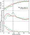 |
Fig. 12 Comparison of the profile of CL J1226.9+3332 in the region of the GGM ridge (green) to its complement (red). The GGM ridge region is define in Fig. 9, as the black dashed line on the surface brightness image. The dashed-dotted line correspond to the GGM ridge location. Top: surface brightness profile. Middle: GGM profile. Bottom: Chandra photon count per unit area profile. |
7 Discussions and perspectives
Cosmological studies using tSZ observations of clusters of galaxies generally rely on mass estimates based on various hypotheses, such as the hydrostatic equilibrium of the ICM or the 3D structure for lensing masses, and the self-similarity of the galaxy cluster population. These assumptions enable a calibration of the scaling law linking the integrated Compton parameter to the cluster total mass (see, e.g, Arnaud et al. 2007, 2010; Planck Collaboration Int. V 2013), and using a universal pressure profile to compute thetSZ power spectrum (e.g., Komatsu & Seljak 2002). However, deviations from these hypotheses have already been identified and may lead to biases on cosmological parameters estimated using galaxy clusters (see, e.g., Ichikawa et al. 2013; McDonald et al. 2014; Planck Collaboration XX 2014; Planck Collaboration XXIV 2016; Planck Collaboration XXII 2016).
Deviations from hydrostatic equilibrium are expected for unrelaxed clusters where the non-thermal pressure content due to turbulence and bulk flows contributes significantly to the equilibrium of the gas in the gravitational potential (e.g., Siegel et al. 2016). Such effects suppress power principally on large scales in the tSZ power spectrum whereas AGN feedback has a significant impact on small scales (e.g., Shaw et al. 2010). Furthermore, the bias affecting the estimate of the cluster mass under the hydrostatic equilibrium assumption in unrelaxed clusters is expected to be higher than for relaxed clusters. The complex inner structure that can arise in the case of disturbed clusters can also affect lensing mass estimates. In this context, dynamical state indicators such as the features identified by the GGM and DoG filters are powerful tools to identify unrelaxed gas structures, which can help to understand the scatter and offset in the scaling relations.
While the tSZ surface brightness map of a cluster subject to AGN feedback can display an apparent relaxed morphology (see the cluster RG448_00211 in Fig. 4), the GGM map of this system reveals a characteristic ring feature which is not observed for a fully relaxed cluster (see the cluster RG361_00188 in the same figure). The GGM map can then be used as a dynamical indicator to identify unrelaxed ICM regions in cluster outskirts and could therefore be linked to the amplitude of the hydrostatic bias.
Information on the dynamical state of the ICM is also given by the comparison of the distinct projected distributions of gas and dark matter. In the case of relaxed systems such as RG361_00188, the gas distribution follows that of the dark matter density, contrarily to major mergers or clusters with disturbed outskirts. Although the tSZ surface brightness map does not enable one to constrain the dark matter density distribution, the gas compression direction provided by both the GGM and DoG maps can provide information on the projected shape of the underlying gravitational potential. For example, while the apparent ICM morphology of the cluster RG448_00211 in Fig. 4 is azimuthally symmetric, the DoG map of this cluster displays an elliptical morphology with a major axis direction matching the one of the dark matter density distribution. The features in the DoG filter maps can therefore be used as a morphology indicator to identify potential deviations between the gas and the dark matter distribution.
Constraining the distribution of the cluster merger rate in large ranges of halo mass and redshift is of key importance to improve our understanding of the formation of large-scale structures (e.g., Fakhouri et al. 2010). The GGM map of the head-on merger RG474_00172 (see Fig. 5) displays a characteristic bimodal distribution giving the locations of high gas compression. Such information is not provided by the tSZ surface brightness map obtained after the end-to-end processing of the RHAPSODY-G simulated cluster. The GGM filter could therefore be used to improve on the identification of mergers by discriminating relaxed elongated ICM and major mergers.
The gas compression intensity, given by the amplitude of the gradient in the GGM maps, could also be compared to radio relic observations (e.g., van Weeren et al. 2010). The identification of a correlation between the two observables would enable to link the amplitude of the gradient in the GGM maps to the Mach number. Such information would greatly enhance the understanding of structure assembly especially when combined with the gas line of sight velocity provided by kSZ effect observations.
8 Summary and conclusions
The tSZ effect provides a direct observable for the ICM pressure in galaxy clusters. In order to search for pressure substructures, which are related to the formation history of the clusters, we have applied filtering methods to resolved NIKA tSZ maps of six galaxy clusters at intermediate and high redshift. The same methods were applied to toy models and to the RHAPSODY-G hydrodynamical simulations in order to better interpret our results. Additionally, a careful investigation of the impact of possible systematic effects was performed. We considered contamination from compact sources, the filtering due to the NIKA processing, and the propagation of the spatially correlated noise.
While half of the clusters in the NIKA sample do not present sufficiently high S/N to enable the identification of internal pressure structures with confidence, the three others show significant features that are not visible in the raw tSZ maps. The observed structures show signatures that are similar to the ones observed in the RHAPSODY-G simulations where they can be clearly attributed to compressions and shocks in the hot gas due to merging events. The potential point source residual contamination is unlikely to cause such structures because its signature is different from the one we observe, and expected to be subdominant. Similarly, we find that the effects of the NIKA processing are not significant at the scales of the observed structures and are subdominant given the available S/N. Finally, we account for spatial correlations of the noise in order to assess the significance of the detections.
The three clusters with the highest S/N in our sample, MACS J0717.5+3745 at z = 0.54, PSZ1 G045.85+57.71 at z= 0.61 and CL J1226.9+3332 at z = 0.89, were investigated in more depth. MACS J0717.5+3745 is clearly disturbed at all scales probed by NIKA. Three strong pressure gradient features are observed in the northwest, east, and southeast sectors, using the GGM filter. We also identified two main peaks in the pressure distribution from the DoG filtered map, which are associated with sub-groups seen at other wavelengths. PSZ1 G045.85+57.71 is elongated on large scales, but we do not observe significant sub-clumps. A GGM ridge is observed in the southeast of the cluster, potentially indicating ongoing merging activity. CL J1226.9+3332 appears to be relaxed on large scales, but the GGM filtered map shows a ~ 45 arcsec (360 kpc) long GGM ridge in the west region associated with an elongation of the gas on small scales as observed in the DoG filtered map. Its signature is in excellent agreement with that of a shock.
The combined high angular resolution and high sensitivity of current tSZ data has now reached a state where the detailed study of the ICM structure of galaxy clusters is possible up to intermediate and high redshifts. In the case of our sample, significant substructures start to be visible for clusters with a peak S/N of ≳ 10 per ~ 22 arcsec beam.
Our analysis shows that it is possible to explore the details of cluster assembly in distant clusters using deep tSZ imaging. New-generation instruments, such as NIKA2 (Calvo et al. 2016; Catalano et al. 2016; Adam et al. 2018) at the IRAM 30 m telescope, are expected to provide unprecedented high-sensitivity tSZ data at high angular resolution. NIKA2 observations (such as the ones of the tSZ large program, Comis et al. 2016; Mayet et al. 2017) should therefore allow for in-depth investigation of the inner structure of the ICM pressure of a cosmologically representative cluster sample. Currently, the sample that we used in this paper is limited to redshifts larger than 0.45, at which the 18 arcsec FWHM NIKA resolution at 150 GHz corresponds to about 100 kpc. With an instantaneous field of view of 6.5 arcmin, NIKA2 will also allow us to observe lower redshift clusters more easily, and thus enable access to smaller physical scales at similar integration time. At intermediate and high redshift, the mapping speed should increase by a factor of up to ~ 10 from NIKA to NIKA2, thus providing very high-S/N images in very short observing time.
Acknowledgements
We are thankful to the anonymous referee for useful comments, which helped improve the quality of the paper. We would like to thank the IRAM staff for their support during the campaigns. The NIKA dilution cryostat has been designed and built at the Institut Néel. In particular, we acknowledge the crucial contribution of the Cryogenics Group, and in particular Gregory Garde, Henri Rodenas, Jean Paul Leggeri, Philippe Camus. This work has been partially funded by the Foundation Nanoscience Grenoble, the LabEx FOCUS ANR-11-LABX-0013 and the ANR under the contracts “MKIDS”, “NIKA” and ANR-15-CE31-0017. This work has benefited from the support of the European Research Council Advanced Grants ORISTARS and M2C under the European Union’s Seventh Framework Programme (Grant Agreement nos. 291294 and 340519). We acknowledge funding from the ENIGMASS French LabEx (B. C. and F. R.), the CNES post-doctoral fellowship program (R. A.), the CNES doctoral fellowship program (A. R.) and the FOCUS French LabEx doctoral fellowship program (A. R.). R.A. acknowledges support from Spanish Ministerio de Economía and Competitividad (MINECO) through grant number AYA2015-66211-C2-2. E. P. acknowledges the support of the French Agence Nationale de la Recherche under grant ANR-11-BS56-015. O.H. acknowledges funding from the European Research Council (ERC) under the European Union’s Horizon 2020 research and innovation programme (grant agreement No 679145, project COSMO_SIMS). D.M. acknowledges support from the Swiss National Science Foundation (SNSF) through the SNSF Early.Postdoc and Advanced.Postdoc Mobility Fellowships.
Appendix A Impact of the filter parameters
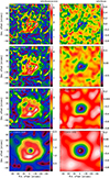 |
Fig. A.1 Evolution of the GGM (left) and DoG (right) filtered maps of CL J1226.9+3332 as a function of the filter parameters. From left to right, the parameters are
|


In Fig. A.1, we provide the extracted filtered signal as a function of the filtering parameters in the case of CL J1226.9+3332. As the size of the filters increases, the detection strength increases, but the small scale signal we aim at extracting becomes washed out. The baseline parameters chosen in this paper correspond to the second row.
Appendix B Transfer function deconvolution
In order to account for the NIKA processing transfer function, we compute the fraction of filtering, as a function of wave number k, by comparing input simulations with known signal (typically cluster toy models that contain signal mostly on large scales, to which we add white noise that contains signal at all scales). We refer to Adam et al. (2015, 2016), for more details on the procedure. The surface brightness images are deconvolved from the filtering by dividing the data by the transfer function in Fourier space. We also refer to the NIKA sample data release web page2, where we provide an IDL script to account for the transfer function. The noise is boosted on large scales, and this is included in our analysis by considering the deconvolved noise Monte Carlo realization when using the deconvolved images. We note that the data processing might generally lead to bouncing artifacts around the brightest signal regions, which could propagate into the filtered maps. However, these effects are strongly mitigated by the masking of the source that is done by iteratively flagging the highest S/N regions (see Adam et al. 2015). Such artifacts remain insignificant with respectto the noise, as shown in Fig. B.1 and discussed below. Further details and more illustrations about the data reduction can be found in the Ph.D. thesis by Adam (2015), in particular in Chapter 7.
The two first columns of Fig. B.1 show the processed surface brightness images before and after deconvolution, in the case of the relatively nearby and very massive test case RHAPSODY-G cluster RG474_00235. This cluster is chosen because of its large angular size on the sky, such that it is the most affected by transfer function effects, and corresponds to an upper limit case with respect to the NIKA clusters. The top row corresponds to a case with S/N peaking at about 20 onthe surface brightness, at 22 arcsec resolution (scaled to the best NIKA detection), and the bottom row to a peak S/N of 4 (the lowest NIKA detection). The three last columns of Fig. B.1 provide the difference maps between the processed data and the true expected maps (see Fig. 4), for the deconvolvedsurface brightness, the GGM filter and the DoG filter. The difference maps are provided in terms of S/N.
shown in Fig. B.1, the differences between the maps are consistent with noise. In the surface brightness map, most of the residual power is on large scales. This is because the noise is boosted by the deconvolution, mainly on large scales, but also becauseof the small inaccuracies in the transfer function that lead to differences between the true initial map and the one we recover. Thelatter is particularly true for this test cluster, in the high-S/N case, because the signal is very large on large scales, where the filtering of the transfer function is important. For the low-S/N case, the effect of errors in the deconvolution has the same amplitude, but is subdominant compared to the noise that is larger. In the case of the GGM and the DoG filters, the scales that we consider are smaller than those where the deconvolution is critical and thus, the maps are not affected significantly by the deconvolution. Both residual maps do not show any structure above the noise, even in the high-S/N regime. In the low-S/N regime, the GGM filter map presents more structure (still well below detection limits) that arise because of inaccuracies in the input map, which is used in the filter (Ŝ in Eq. (8)), as discussed in Sect. 5.3 and shown in Fig. 7.
In summary, the systematic effects introduced by the deconvolution are negligible with respect to the noise, even in the highest-S/N cases available from the NIKA sample. In the low-S/N regime, the deconvolution does not introduce any uncontrolled artifacts. Therefore, systematics associated to the transfer function can be safely neglected in the main paper analysis.
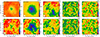 |
Fig. B.1 Effect of the deconvolution on the processed map (first two columns) and difference between the expected signal and the recovered signal (3 last columns), in the case of the very massive and nearby test cluster RG474_00235. The top panel correspond to the high S/N case, and the bottom panel to the low signal-to-noise case, with a peak S/N of about 20 and 3, respectively, at the 22 arcsec resolution. From left to right, we provide: the raw processed surface brightness, the deconvolved surface brightness, the deconvolved surface brightness difference map, the GGM difference map, and the DoG difference map. In all cases, contours provide the S/N, starting at ± 2σ and increasing by 2σ steps. |
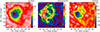 |
Fig. B.2 Surface brightness (left), GGM (middle) and DoG (right) maps of MACS J0717.5+3745 in the case of kSZ correction applied. See Fig. 9 for further details. |
Appendix C Impact of kSZ signal in MACS J0717.5+3745
The surface brightness of MACS J0717.5+3745 is affected by kSZ signal, and it is the only cluster for which an individual kSZ detection has been obtained to date (Mroczkowski et al. 2012; Sayers et al. 2013; Adam et al. 2017b). The kSZ signal is related to the gas density and line-of-sight velocity and has to be considered in order to study the pressure structure via the tSZ signal. Mroczkowski et al. (2012), Sayers et al. (2013) and Adam et al. (2017b) have obtained several kSZ signal models, but they are all limited by the large uncertainties in their best-fit parameters and are subject to strong assumptions in the gas modeling. Therefore, it is only possible to test the impact of the kSZ signal on our result by comparing the recovered substructures in the cases with and without kSZ correction. We thus produce a kSZ clean map of MACS J0717.5+3745 using the best-fit kSZ model from Adam et al. (2017b) to do so. Figure B.2 provides the surface brightness and filtered maps of MACS J0717.5+3745 in the case where the kSZ signal model has been subtracted to the data. The overall structure is similar to that observed in Fig. 9, where no correction is applied, butthe magnitude of the different structures is significantly affected. See Sect. 6.3 for discussions.
References
- Adam, R. 2015, PhD Thesis, Université Grenoble-Alpes, France [Google Scholar]
- Adam, R., Comis, B., Macías-Pérez, J. F., et al. 2014, A&A, 569, A66 [NASA ADS] [CrossRef] [EDP Sciences] [Google Scholar]
- Adam, R., Comis, B., Macías-Pérez, J.-F., et al. 2015, A&A, 576, A12 [NASA ADS] [CrossRef] [EDP Sciences] [Google Scholar]
- Adam, R., Comis, B., Bartalucci, I., et al. 2016, A&A, 586, A122 [NASA ADS] [CrossRef] [EDP Sciences] [Google Scholar]
- Adam, R., Arnaud, M., Bartalucci, I., et al. 2017a, A&A, 606 A64 [NASA ADS] [CrossRef] [EDP Sciences] [Google Scholar]
- Adam, R., Bartalucci, I., Pratt, G. W., et al. 2017b, A&A, 598, A115 [NASA ADS] [CrossRef] [EDP Sciences] [Google Scholar]
- Adam, R., Adane, A., Ade, P. A. R., et al. 2018, A&A, 609, A115 [NASA ADS] [CrossRef] [EDP Sciences] [Google Scholar]
- Allen, S. W., Evrard, A. E., & Mantz, A. B. 2011, ARA&A, 49, 409 [NASA ADS] [CrossRef] [Google Scholar]
- Arnaud, M., Pointecouteau, E., & Pratt, G. W. 2007, A&A, 474, L37 [NASA ADS] [CrossRef] [EDP Sciences] [Google Scholar]
- Arnaud, M., Pratt, G. W., & Piffaretti, R., et al. 2010, A&A, 517, A92 [NASA ADS] [CrossRef] [EDP Sciences] [Google Scholar]
- Basu, K., Sommer, M., & Erler, J., et al. 2016, ApJ, 829, L23 [NASA ADS] [CrossRef] [Google Scholar]
- Birkinshaw, M. 1999, Phys. Rep., 310, 97 [NASA ADS] [CrossRef] [Google Scholar]
- Böhringer, H., Schuecker, P., Pratt, G. W., et al. 2007, A&A, 469, 363 [NASA ADS] [CrossRef] [EDP Sciences] [Google Scholar]
- Bourdin, H., Mazzotta, P., & Rasia, E. 2015, ApJ, 815, 92 [NASA ADS] [CrossRef] [Google Scholar]
- Calvo, M., Benoît, A., Catalano, A., et al. 2016, J. Low Temp. Phys., 184, 816 [NASA ADS] [CrossRef] [Google Scholar]
- Catalano, A., Calvo, M., Ponthieu, N., et al. 2014, A&A, 569, A9 [NASA ADS] [CrossRef] [EDP Sciences] [Google Scholar]
- Catalano, A., Adam, R., Ade, P., et al. 2016, ArXiv e-prints, [arXiv:1605.08628] [Google Scholar]
- Comis, B., Adam, R., Ade, P., et al. 2016, ArXiv e-prints, [arXiv:1605.09549] [Google Scholar]
- Dicker, S. R., Ade, P. A. R., Aguirre, J., et al. 2014, in Millimeter, Submillimeter, and Far-Infrared Detectors and Instrumentation for Astronomy VII, Proc. SPIE, 9153, 91530J [NASA ADS] [CrossRef] [Google Scholar]
- Ebeling, H., Jones, L. R., & Fairley, B. W., et al. 2001, ApJ, 548, L23 [NASA ADS] [CrossRef] [Google Scholar]
- Fabian, A. C. 2012, ARA&A, 50, 455 [NASA ADS] [CrossRef] [Google Scholar]
- Fabian, A. C., Sanders, J. S., Allen, S. W., et al. 2003, MNRAS, 344, L43 [NASA ADS] [CrossRef] [Google Scholar]
- Fakhouri, O., Ma, C.-P., & Boylan-Kolchin, M. 2010, MNRAS, 406, 2267 [NASA ADS] [CrossRef] [Google Scholar]
- Hahn, O., Martizzi, D., & Wu, H.-Y., et al. 2017, MNRAS, 470, 166 [NASA ADS] [Google Scholar]
- Ichikawa, K., et al. 2013, ApJ, 766, 90 [NASA ADS] [CrossRef] [Google Scholar]
- Itoh, N., & Nozawa, S. 2003, ArXiv e-prints, [arXiv:astro-ph/0307519] [Google Scholar]
- Jee, M. J., & Tyson, J. A. 2009, ApJ, 691, 1337 [NASA ADS] [CrossRef] [Google Scholar]
- Kitayama, T., Komatsu, E., Ota, N., et al. 2004, PASJ, 56, 17 [NASA ADS] [Google Scholar]
- Kitayama, T., Ueda, S., Takakuwa, S., et al. 2016, PASJ, 68, 88 [NASA ADS] [CrossRef] [Google Scholar]
- Komatsu, E., & Seljak, U. 2002, MNRAS, 336, 1256 [NASA ADS] [CrossRef] [Google Scholar]
- Komatsu, E., Kitayama, T., Suto, Y., et al. 1999, ApJ, 516, L1 [NASA ADS] [CrossRef] [Google Scholar]
- Korngut, P. M., Dicker, S. R., Reese, E. D., et al. 2011, ApJ, 734, 10 [NASA ADS] [CrossRef] [Google Scholar]
- Kravtsov, A. V., & Borgani, S. 2012, ARA&A, 50, 353 [NASA ADS] [CrossRef] [Google Scholar]
- Kreisch, C. D., Machacek, M. E., Jones, C., & Randall, S. W. 2016, ApJ, 830, 39 [NASA ADS] [CrossRef] [Google Scholar]
- Limousin, M., Richard, J., Jullo, E., et al. 2016, A&A, 588, A99 [NASA ADS] [CrossRef] [EDP Sciences] [Google Scholar]
- Ma, C.-J., Ebeling, H., & Barrett, E. 2009, ApJ, 693, L56 [NASA ADS] [CrossRef] [Google Scholar]
- Markevitch, M., & Vikhlinin, A. 2007, Phys. Rep., 443, 1 [NASA ADS] [CrossRef] [EDP Sciences] [Google Scholar]
- Mason, B. S., Dicker, S. R., Korngut, P. M., et al. 2010, ApJ, 716, 739 [NASA ADS] [CrossRef] [Google Scholar]
- Maughan, B. J., Jones, C., Jones, L. R., & Van Speybroeck, L. 2007, ApJ, 659, 1125 [NASA ADS] [CrossRef] [Google Scholar]
- Mayet, F., Adam, R., Ade, P.,et al. 2017, ArXiv e-prints [arXiv:1709.01255] [Google Scholar]
- McDonald, M., Benson, B. A., Vikhlinin, A., et al. 2014, ApJ, 794, 67 [NASA ADS] [CrossRef] [Google Scholar]
- Monfardini, A., Benoit, A., Bideaud, A., et al. 2011, ApJS, 194, 24 [NASA ADS] [CrossRef] [Google Scholar]
- Mroczkowski, T., Dicker, S., Sayers, J., et al. 2012, ApJ, 761, 47 [NASA ADS] [CrossRef] [Google Scholar]
- Nagai, D., Vikhlinin, A., & Kravtsov, A. V. 2007, ApJ, 655, 98 [NASA ADS] [CrossRef] [Google Scholar]
- Plagge, T. J., Marrone, D. P., Bonamente, Z, et al. 2013, ApJ, 770, 112 [NASA ADS] [CrossRef] [Google Scholar]
- Planck Collaboration XX 2014, A&A, 571, A20 [NASA ADS] [CrossRef] [EDP Sciences] [Google Scholar]
- Planck Collaboration XXIX 2014, A&A 571, A29 [NASA ADS] [CrossRef] [EDP Sciences] [Google Scholar]
- Planck Collaboration XIII 2016, A&A, 594, A13 [NASA ADS] [CrossRef] [EDP Sciences] [Google Scholar]
- Planck Collaboration XXIV 2016, A&A, 594, A24 [NASA ADS] [CrossRef] [EDP Sciences] [Google Scholar]
- Planck Collaboration XXII 2016, A&A, 594, A22 [NASA ADS] [CrossRef] [EDP Sciences] [Google Scholar]
- Planck Collaboration XXVII 2016, A&A, 594, A27 [NASA ADS] [CrossRef] [EDP Sciences] [Google Scholar]
- Planck Collaboration Int. V 2013, A&A, 550, A131 [NASA ADS] [CrossRef] [EDP Sciences] [Google Scholar]
- Pointecouteau, E., Giard, M., Benoit, A., et al. 1999, ApJ, 519, L115 [NASA ADS] [CrossRef] [Google Scholar]
- Pointecouteau, E., Giard, M., Benoit, A., et al. 2001, ApJ, 552, 42 [NASA ADS] [CrossRef] [Google Scholar]
- Pratt, G. W., Arnaud, M., Piffaretti, R., et al. 2010, A&A, 511, A85 [NASA ADS] [CrossRef] [EDP Sciences] [Google Scholar]
- Roediger, E., Kraft, R. P., Forman, W. R., Nulsen, P. E. J., & Churazov, E. 2013, ApJ, 764, 60 [NASA ADS] [CrossRef] [Google Scholar]
- Romero, C., McWilliam, M., Mac"i"as-Perez, J.-F., et al. 2018, A&A, 612, A39 [NASA ADS] [CrossRef] [EDP Sciences] [Google Scholar]
- Ruppin, F., Adam, R., Comis, B., et al. 2017, A&A, 597, A110 [NASA ADS] [CrossRef] [EDP Sciences] [Google Scholar]
- Sanders, J. S., Fabian, A. C., Russell, H. R., Walker, S. A., & Blundell, K. M. 2016a, MNRAS, 460, 1898 [NASA ADS] [CrossRef] [Google Scholar]
- Sanders, J. S., Fabian, A. C., Taylor, G. B., et al. 2016b, MNRAS, 457, 82 [NASA ADS] [CrossRef] [Google Scholar]
- Sarazin, C. L. 2002, in Merging Processes in Galaxy Clusters, eds. L. Feretti, I. M. Gioia, & G. Giovannini, Astrophys. Space Sci. Lib., 272, 1 [NASA ADS] [Google Scholar]
- Sayers, J., Mroczkowski, T., Zemcov, M., et al. 2013, ApJ, 778, 52 [NASA ADS] [CrossRef] [Google Scholar]
- Sayers, J., Zemcov, M., Glenn, J., et al. 2016, ApJ, 820, 101 [NASA ADS] [CrossRef] [Google Scholar]
- Shaw, L. D., Nagai, D., Bhattacharya, S., & Lau, E. T. 2010, ApJ, 725, 1452 [NASA ADS] [CrossRef] [Google Scholar]
- Siegel, S. R., et al. 2016, ArXiv e-prints [arXiv:1612.05377] [Google Scholar]
- Sunyaev, R. A., & Zel’dovich, Y. B. 1972, Astrophys. Space Phys. Res., 4, 173 [Google Scholar]
- Sunyaev, R. A., & Zeldovich, I. B. 1980, MNRAS, 190, 413 [NASA ADS] [CrossRef] [Google Scholar]
- van Weeren, R. J., Rottgering, H. J. A., Bruggen, M., & Hoeft, M. 2010, Science, 330, 347 [NASA ADS] [CrossRef] [PubMed] [Google Scholar]
- van Weeren, R. J., Ogrean, G. A., Jones, C., et al. 2017, ApJ, 835, 197 [NASA ADS] [CrossRef] [Google Scholar]
- Wu, H.-Y., Hahn, O., Wechsler, R. H., Mao, Y.-Y., & Behroozi, P. S. 2013, ApJ, 763, 70 [NASA ADS] [CrossRef] [Google Scholar]
The three-digit number after “RG” refers to the respective RHAPSODY-G halo, while the second five-digit number refers to the snapshot number of the analyzed map.
All Tables
Summary of the main properties of the NIKA cluster sample, ordered by increasing redshift.
All Figures
|
Fig. 1 Example of the raw surface brightness image of MACS J0717.5+3745, prior to any filter application (e.g., smoothing), point source removal and deconvolution. The data is dominated by noise on small scales. The cluster diffuse emission is nonetheless visible as a negative decrement, as well as a radio foreground galaxy (positive) on the southeast. The white circle on the bottom left corner provide the NIKA beam FWHM. |
| In the text | |
|
Fig. 2 Surface brightness and GGM and DoG response to the tSZ signal expected for a spherically symmetric gNFW pressure profile (top), a bimodal cluster plus a pressure bar (middle), and a main core plus an extension (bottom). Left: tSZ simulated surface brightness. The white circle on the bottom left provides the beam FWHM. Middle: GGM filtered maps with θ0 = 15′′. The white vectors represent the direction of the gradient, Ψ. Right: DoG filtered maps with θ1 = 15′′ and θ2 = 45′′. |
| In the text | |
|
Fig. 3 Left: GGM and DoG response to a gNFW radial pressure profile. The vertical dashed line provides the physical size corresponding to the 15 arcsec filter plus the NIKA beam size, at the cluster redshift. Right: GGM and DoG response to a shock propagating outward, in a radially symmetrical way, with Mach number
|
| In the text | |
|
Fig. 4 Application of the filtering algorithms to clusters from the RHAPSODY-G suite of simulations. From top to bottom, the clusters are RG361_00188, RG474_00172, RG377_00181, RG448_00211, and RG474_00235 (see also Table 2 for the main properties of the sample). Left: projected dark matter density. Contours are linearly spaced. Units are arbitrary. Middle left: input raw tSZ surface brightness maps with dark matter map contours overlaid. Units are mJy beam−1. Middle right: GGM filtered maps with θ0 = 15′′. The white vectors represent the direction of the gradient, Ψ. Units are mJy beam−1 arcmin−1. Right: DoG filtered maps with θ1 = 15′′ and θ2 = 45′′. Units are mJy beam−1. The contours provide the true S/N expected for the simulation of the observation of these sources done in Sect. 5. They are given by steps of 2σ excluding 0 (see Sect. 5 for further discussions about the S/N estimates). |
| In the text | |
|
Fig. 5 As in Fig. 4 but for the case of end-to-end processing of the simulated RHAPSODY-G sub-sample: surface brightness maps (left), GGM filtered maps (middle) and DoG filtered maps (right). From top to bottom, the clusters areRG361_00188, RG474_00172, RG377_00181 and RG448_00211 (see also Table 2 for the main properties of the sample). The surface brightness images are deconvolved from the transfer function (but not from the beam smoothing) and the S/N contours are estimated as in the case of real data (separated by steps of 2σ). |
| In the text | |
|
Fig. 6 Noise distribution of all the pixels enclosed within 30 arcsec radius from the cluster center, in the case of CL J1226.9+3332, for our baseline filter parameters. The red curves provide the best Gaussian fit to the histograms. Left: DoG noise histogram. Middle: GGM noise histogram in the case of Ŝ set to the observed signal of CL J1226.9+3332. Right: GGM noise histogram in the case where Ŝ = 0 in Eq (8). |
| In the text | |
|
Fig. 7 Comparison of the estimated GGM filtered maps S/N as a function of the true S/N, using the RHAPSODY-G sub-sample. The estimated S/N is computed using the NIKA processed RHAPSODY-G sub-sample (Eq. (9)). The red dashed line represent the one to one correspondence. Each point corresponds to a pixel of the map. |
| In the text | |
|
Fig. 8 Application of the filters to point source residuals in case 1 (no source subtraction, top) and case 2 (source improperly subtracted, bottom). The input point source flux has been normalized to one. Left: input surface brightness map. Middle: GGM filtered map. Right: DoG filtered map. |
| In the text | |
|
Fig. 9 Redshift-ordered maps of the NIKA cluster sample at 150 GHz. Left: surface brightness images. Each map has been smoothed to an effective angular resolution of 22 arcsec FWHM, as shown by the bottom left white circle. Point sources have been subtracted and the data have been deconvolved from the transfer function, but the zero level absolute brightness remains unconstrained. Middle: GGM filtered maps. Right: DoG filtered maps. In all cases, contours provide the S/N, starting at ± 2σ and increasing by 2σ steps. The white crosses provide the main X-ray peak (see Table 3). In the case of MACS J0717.5+3745, the kSZ contribution is not accounted for in the map presented here (see Appendix C and Sect. 6.3 for more details). In the case of CL J1226.9+3332 and MACS J0717.5+3745, the dashed lines correspond to the cone used to define the GGM ridge region when extracting profiles in Figs. 12 and 11. |
| In the text | |
|
Fig. 10 Multi-probe view of the cluster MACS J0717.5+3745: Chandra X-ray surface brightness image (ObsID4200), plotted on a square root scale (thus proportional to the projected density) with XMM-Newton temperature (green contours from Adam et al. 2017a) and the DoG (black contours) and GGM (white contours) maps overlaid. |
| In the text | |
|
Fig. 11 Profile of MACS J0717.5+3745 in the region defined to include the strongest GGM ridge (east ridge, see Fig. 9, as the dark gray dashed line on the surface brightness image). The dashed-dotted line correspond to the GGM ridge location. Top: surface brightness profile. Middle: GGM profile. Bottom: Chandra photon count per unit area profile. |
| In the text | |
|
Fig. 12 Comparison of the profile of CL J1226.9+3332 in the region of the GGM ridge (green) to its complement (red). The GGM ridge region is define in Fig. 9, as the black dashed line on the surface brightness image. The dashed-dotted line correspond to the GGM ridge location. Top: surface brightness profile. Middle: GGM profile. Bottom: Chandra photon count per unit area profile. |
| In the text | |
|
Fig. A.1 Evolution of the GGM (left) and DoG (right) filtered maps of CL J1226.9+3332 as a function of the filter parameters. From left to right, the parameters are
|
| In the text | |
|
Fig. B.1 Effect of the deconvolution on the processed map (first two columns) and difference between the expected signal and the recovered signal (3 last columns), in the case of the very massive and nearby test cluster RG474_00235. The top panel correspond to the high S/N case, and the bottom panel to the low signal-to-noise case, with a peak S/N of about 20 and 3, respectively, at the 22 arcsec resolution. From left to right, we provide: the raw processed surface brightness, the deconvolved surface brightness, the deconvolved surface brightness difference map, the GGM difference map, and the DoG difference map. In all cases, contours provide the S/N, starting at ± 2σ and increasing by 2σ steps. |
| In the text | |
|
Fig. B.2 Surface brightness (left), GGM (middle) and DoG (right) maps of MACS J0717.5+3745 in the case of kSZ correction applied. See Fig. 9 for further details. |
| In the text | |
Current usage metrics show cumulative count of Article Views (full-text article views including HTML views, PDF and ePub downloads, according to the available data) and Abstracts Views on Vision4Press platform.
Data correspond to usage on the plateform after 2015. The current usage metrics is available 48-96 hours after online publication and is updated daily on week days.
Initial download of the metrics may take a while.