| Issue |
A&A
Volume 613, May 2018
|
|
|---|---|---|
| Article Number | A11 | |
| Number of page(s) | 26 | |
| Section | Interstellar and circumstellar matter | |
| DOI | https://doi.org/10.1051/0004-6361/201731587 | |
| Published online | 16 May 2018 | |
Gravity drives the evolution of infrared dark hubs: JVLA observations of SDC13★
1
School of Physics and Astronomy, Cardiff University,
Queens Buildings, The Parade,
Cardiff
CF24 3AA, UK
e-mail: williamsgwen12@gmail.com
2
Jodrell Bank Centre for Astrophysics, School of Physics and Astronomy, University of Manchester,
Manchester
M13 9PL, UK
3
UK ALMA Regional Centre Node,
Manchester
M13 9PL, UK
Received:
17
July
2017
Accepted:
22
January
2018
Context. Converging networks of interstellar filaments, that is hubs, have been recently linked to the formation of stellar clusters and massive stars. Understanding the relationship between the evolution of these systems and the formation of cores and stars inside them is at the heart of current star formation research.
Aims. The goal is to study the kinematic and density structure of the SDC13 prototypical hub at high angular resolution to determine what drives its evolution and fragmentation.
Methods. We have mapped SDC13, a ~1000 M⊙ infrared dark hub, in NH3(1,1) and NH3(2,2) emission lines, with both the Jansky Very Large Array and Green Bank Telescope. The high angular resolution achieved in the combined dataset allowed us to probe scales down to 0.07 pc. After fitting the ammonia lines, we computed the integrated intensities, centroid velocities and line widths, along with gas temperatures and H2 column densities.
Results. The mass-per-unit-lengths of all four hub filaments are thermally super-critical, consistent with the presence of tens of gravitationally bound cores identified along them. These cores exhibit a regular separation of ~0.37 ± 0.16 pc suggesting gravitational instabilities running along these super-critical filaments are responsible for their fragmentation. The observed local increase of the dense gas velocity dispersion towards starless cores is believed to be a consequence of such fragmentation process. Using energy conservation arguments, we estimate that the gravitational to kinetic energy conversion efficiency in the SDC13 cores is ~35%. We see velocity gradient peaks towards ~63% of cores as expected during the early stages of filament fragmentation. Another clear observational signature is the presence of the most massive cores at the filaments’ junction, where the velocity dispersion is largest. We interpret this as the result of the hub morphology generating the largest acceleration gradients near the hub centre.
Conclusions. We propose a scenario for the evolution of the SDC13 hub in which filaments first form as post-shock structures in a supersonic turbulent flow. As a result of the turbulent energy dissipation in the shock, the dense gas within the filaments is initially mostly sub-sonic. Then gravity takes over and starts shaping the evolution of the hub, both fragmenting filaments and pulling the gas towards the centre of the gravitational well. By doing so, gravitational energy is converted into kinetic energy in both local (cores) and global (hub centre) potential well minima. Furthermore, the generation of larger gravitational acceleration gradients at the filament junctions promotes the formation of more massive cores.
Key words: stars: formation / stars: massive / ISM: clouds / ISM: kinematics and dynamics / ISM: structure
The FITS files of the JVLA and GBT combined NH3(1,1) and NH3(2,2) data cubes are also available at the CDS via anonymous ftp to cdsarc.u-strasbg.fr (130.79.128.5) or via http://cdsarc.u-strasbg.fr/viz-bin/qcat?J/A+A/613/A11
© ESO 2018
1 Introduction
The star formation process can be perceived as the mechanism leading to the concentration of diffuse interstellar clouds into compact, nuclear burning, balls of gas. While the importance of interstellar filaments had been recognised already in the seventies (Schneider & Elmegreen 1979), observations of the Galactic interstellar medium with Herschel have revealed that they are a key intermediate stage towards the formation of stars (André et al. 2010; Molinari et al. 2010; Arzoumanian et al. 2011). Indeed, the majority of pre-stellar and proto-stellar cores are embedded in thermally supercritical filaments (Polychroni et al. 2013; Könyves et al. 2015; Marsh et al. 2016), that is filaments whose mass-per-unit-length Mline is larger than the theoretical upper limit for an isothermal, infinitely long cylinder to maintain hydrostatic equilibrium (Ostriker 1964). Understanding the connection between filament evolution and core formation has become one of the main goals of star formation research over the past decade.
While a lot of effort has focused on the properties of individual filaments in nearby star-forming regions (Arzoumanian et al. 2011; Peretto et al. 2012; Palmeirim et al. 2013; Panopoulou et al. 2014; Salji et al. 2015), here we focus on hub filament systems (HFS), i.e. a small network of spatially converging interstellar filaments (Myers 2009). The converging nature of such systems is suggestive of the role played by gravity in shaping them. Follow-up observations have shown that hubs are likely collapsing on parsec scales, gathering matter at their centre as a result of the collapse (Kirk et al. 2013; Peretto et al. 2013, 2014; Liu et al. 2013). One of the most massive proto-stellar cores ever observed in the Galaxy has been found lying at the centre of such hubs (Peretto et al. 2013), indicating that they might play a key role in the formation of massive stars. Schneider et al. (2012) also showed that stellar protoclusters in the Rosette molecular cloud tend to form at the junctionof filamentary structures. Understanding how hubs form and evolve can tell us what physical mechanisms are behind the fragmentation of filaments and how their interaction influence the formation of more massive objects. High-angular resolution observationsof infrared dark clouds (IRDCs) provides us with the opportunity to study such systems very early on in their evolution.
IRDCs are cold (T < 20 K) and dense (n > 103 cm−3) reservoirs ofgas seen in extinction against the bright mid-infrared emission of the Galactic plane background (Perault et al. 1996; Egan et al. 1998; Simon et al. 2006; Peretto & Fuller 2009; Butler & Tan 2009; Peretto et al. 2010). They are considered to be mostly undisturbed by stellar feedback due to the lack of a significant embedded population of stars, and exhibit a wide range of morphologies, masses and sizes (Peretto et al. 2010). The most massive of these IRDCs are thought to contain the initial conditions for massive star formation (Rathborne et al. 2006; Pillai et al. 2006; Beuther & Steinacker 2007).
SDC13 (Fig. 1) is a remarkable filamentary hub IRDC system that lies 3.6 ± 0.4 kpc away in the Galactic plane and contains ~ 1000 M⊙ of material (Peretto et al. 2014). Each of its four well-defined parsec-long filaments (including SDC13.174−0.07, SDC13.158−0.073 and SDC13.194−0.073, Peretto & Fuller 2009, subsequently named following their on-sky orientation) converges on a central hub. With the analysis of 1.2 mm dust continuum data from the MAMBO bolometer array on the IRAM 30m telescope (at 12″ resolution) 18 compact sources were extracted and their starless or proto-stellar nature identified from 8 μm and 24 μm Spitzer images. The two most massive cores (named MM1 and MM2) are located right at the junction of the hub filaments, the substructure of which was studied using high resolution (< 3″) 1.3 mm SMA dust continuum emission (McGuire et al. 2016). MM1 was found to contain two subfragments, the centremost being brighter than the MM2 fragment. Modelling the cores with RADMC-3D reveals that MM2 requires a steeper density profile than MM1, suggesting that it may be most likely to form a single massive central object (Girichidis et al. 2011). Tracing the dense gas in N2 H+(1–0) with the IRAM 30 m telescope (at 27″ resolution) Peretto et al. (2014) identified velocity gradients along each of the filamentary arms of SDC13. Infall velocities larger at the filament ends anti-correlate with the velocity dispersion gradients which reach their maximum at the hub centre. This was interpreted as the consequenceof the collapse of the gas along the filaments, generating an increase of kinetic pressure at the centre of the hub and providing the necessary conditions for the formation of super-Jeans cores, i.e. cores with masses that are several times larger than the local Jeans mass.
In this paper we present new high-resolution ammonia observations of SDC13 obtained with the Jansky Very Large Array (JVLA) andthe Green Bank Telescope (GBT). These observations allow us to resolve, for the first time, the density structure and kinematics of the SDC13 filaments, expanding on the analysis of previous work. In Sect. 2 we present the observationsand discuss the process of combining the two data sets. Section 3 presents our line fitting and analysis of the observed kinematics of the system. In Sect. 4 we discuss the identification of filament and core structures. We discuss the fragmentation and dynamics of the system in Sect. 5, and finally, we summarise our conclusions in Sect. 6.
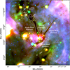 |
Fig. 1 Three colour image of SDC13. R, G and B bands correspond to 70 μm HIGAL (Molinari et al. 2010), 24 μm Spitzer MIPSGAL (Carey et al. 2009) and 8 μm Spitzer GLIMPSE (Churchwell et al. 2009) maps, respectively. The overplotted contour is from the H2 column density map at 2 × 1022 cm−2 (see Sect. 3.2 and the middle panel of Fig. 5). A 1 pc scale bar is plotted in the bottom right corner. The filament names are labelled following those used by Peretto et al. (2014). |
2 Observations
We observedammonia (NH3) at the position of SDC13 with both the JVLA and the GBT. NH3 is rather abundant in star forming regions (Cheung et al. 1968), with an abundance of [NH3]∕[H2] ~ 3 × 10⁻⁸ (Harju et al. 1993). The (J, K) = (1, 1) and (2,2) rotation inversion transitions with their relatively large critical density (ncrit = 103 cm−3, Ho & Townes 1983; Shirley 2015) are particularly good tracers of the cold and dense gas during the early stages of star formation as they are excited at the low temperatures (<20 K) of molecularclouds and IRDCs, and exhibit very little, if any, depletion. Studies of the hyperfine splitting of the (1,1) and (2,2) transitions (e.g. Gunther-Mohr 1954; Kukolich 1967) show that they have 18 and 24 hyperfine components, emitting in the radio regime at 23.69 and 23.72 GHz, respectively (e.g. Ho & Townes 1983). The detection of both these lower metastable states allows for the direct calculation of the opacity, temperature and column density of the gas (e.g. Ho & Townes 1983; Ungerechts et al. 1986).
2.1 JVLA observations
The NH3(1,1) and NH3(2,2) transitions were observed at the position of the SDC13 infrared dark cloud (J2000 18:14:30.0–17:32:50.0) at 23.7 GHz using the JVLA in the DnC configuration, using the 1 GHz band with 4 MHz sub-bands. We observed the NH3 (3,3) transition, but it was not significantly detected. The angular resolution achieved of 3.3″ is an 8-fold improvement on the 27″ resolution of the N2 H+(1–0) molecular line IRAM 30 m data (Peretto et al. 2014), probing 0.07 pc spatial scales. A mosaic across the full 5′ × 5′ extent of the cloud was performed in eight, half-beam spaced pointings, collected over 8 observing sessions between 18 and 20 of May 2013, with 102.4 min integration time per position. Further information on these data are provided in Table 1.
Data reduction and calibration was completed using CASA1 (McMullin et al. 1992). Phase and flux calibration was completed using the two bright quasars J1832−1035 and 3C286, respectively. The phase calibrator was chosen to sit within 6° to the target on the sky to ensure similar atmospheric conditions. Bandpass calibration was completed with the J1743−0350 quasar. We flagged any bad data using the flagcmd() and flagdata() tasks within CASA, and imaged both NH3 transitions using the deconvolution task, clean(). Our imaging implements the Natural weighting scheme, which puts less emphasis on the smallest scale coverage of the data. This was done as our u–v coverage was slightly stretched in this regime due to the low declination of the source.
Summary of the observational properties of the JVLA, GBT and combined data.
2.2 GBTobservations
We used the 7-beam K-band Focal Plane Array at the GBT with the VEGAS (Versatile GBT Astronomical Spectrometer) backend to observe the NH3 (1,1) and (2,2) transitions employing a position switched scheme, where the Off source reference position (18:13:59.3–17:35:02.0) was devoid of NH3 emission. Two maps were scanned in right ascension, while another two were scanned in declination so as to mitigate any artefacts that could arise during imaging had only one mapping scheme been used. All four maps were observed on 14 November 2015, each with an integration time of 17.9 min (see Table 1 for data properties). We ran the GBT pipeline (Masters et al. 2011) on each map scan separately to calibrate, reduce and subtract the continuum emission. All scans were then combined and imaged in AIPS using the aipspy ParselTongue scripts included with the pipeline. Possible issues with the noise diode voltages at the time of observation skewed our flux calibration but had no effect on the quality of the data. This resulted in the measured flux of the flux calibrator (J1833−2103, a quasar) to be lower than expected from published calibration tables. We applied an appropriate calibration factor (a ratio of the expected to the measured flux) to our data to correct for this.
2.3 Combination of JVLA and GBT data
Interferometers only probe a limited range of spatial frequencies of the source brightness spatial distribution, the largest frequency being determined by the shortest distance between any pair of the interferometer antennas. As a consequence, interferometers filter out extended emission. In order to recover this large-scale emission, and therefore be able to analyse the source structure on all spatial scales, one needs to combine interferometer data with single dish data. Hence, we combined our JVLA data with the GBT observations.
As a preliminary combination step, we re-clean our JVLA visibilities in the same way as described in Sect. 2.1, whilst using the GBT cube as a starting model (Dirienzo et al. 2015). This method assists in initializing the clean algorithm by using the GBT primary beam to determine the flux scale. Moreover, as the JVLA is missing information at the shortest baselines, this approach allows the clean algorithm to extrapolate the GBT data and converge on a better solution in this u–v regime. We note that this is not the same as performing a joint deconvolution.
Combination is achieved with the use of the CASA task, feather. With the high and low resolution images as inputs, feather Fourier transforms the two cubes, applies a low-pass filter to the low resolution data and a high-pass filter to the high resolution data, sums the two Fourier and filtered cubes in u–v space, and reconvolves the final combined cube. The low and high pass filters (weights calculated from the input clean beams) are applied to recover the larger scale emission of the GBT data at low u–v distances which the JVLA naturally filters out, whilst retaining the fine scale structure probed by the JVLA at larger u–v distances which the GBT cannot be sensitive to. The primary beam response of the JVLA was applied to the GBT data prior to feathering, so that only emission within the JVLA mosaic area was considered.
The casafeather visual interface provides the tools to inspect slices of the u–v plane of both the original and weighted deconvolved input images. This is especially useful while setting the sdfactor parameter, which applies a flux scaling factor to the low resolution image. For the conservation of flux, one would expect the fluxes of the weighted deconvolved high and low resolution images to be roughly equal. One can achieve this by altering the sdfactor until the casafeather plots demonstrate this equality. Given the uncertainty in the flux calibration of the GBT, we expected a factor would be required, however, we find a satisfactory result with the default sdfactor of 1. This demonstrates that the calibration factor applied to the GBT data in the first instance was sound and appropriate.
Figure 2 shows a comparison of the GBT, JVLA and combined integrated intensity maps of NH3 (1,1). It is clear that the combined data recovers more extended flux than the JVLA-only, resulting in a doubling of the JVLA flux on the whole, whilst retaining the small scale detail and RMS noise of the interferometer. We can clearly see that the negative bowl features, a consequence of missing flux, that surrounds the cloud structure in the JVLA-only map are mostly eradicated in the combined map and filled by the recovered extended emission. A check was made on the conservation of flux, performed by smoothing the feathered image to the resolution of the GBT, converting the units to Jy per GBT beam, and dividing by the original GBT map. In doing this, we find that flux is conserved. In the filament regions, we find a ratio of unity on the whole, whilst in the regions of significant emission such as the hub the combined flux is typically ~20% less than the GBT map (a similar result to that reported by Dirienzo et al. 2015).
In order to gain in signal to noise ratio we convolved the combined datacube with a Gaussian kernel of 2.4″, degrading the angular resolution to ~4″.
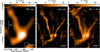 |
Fig. 2 Comparison between the integrated intensity maps of the NH3(1,1) emission from the GBT (left), the JVLA (middle) and the combined GBT and JVLA (right) data sets. The GBT map displayed here has already had the calibration factor applied (see Sect. 2.2). The beam sizes are plotted in the bottom right corner of each panel. A parsec scale at the distance of the cloud is plotted in the first panel. |
3 Results
Here we present the results obtained from fitting the NH3 hyperfine structure, and from deriving a H2 column density map from the NH3 emission.
3.1 Line fitting
We performed hyperfine structure fitting of the combined JVLA and GBT data using the NH3(1,1) and NH3(2,2) fitting schemes within the CLASS2 software, where the spectra are fitted at every pixel over all channels. Figure 3 shows examples of ten spectra and their hyperfine structure fits from positions distributed across the cloud. After visual inspection, we do not find multiple velocity components, even at the filament junctions in the hub centre, therefore we proceed to fit a single velocity component everywhere. Using the result command, a model fit to the data was created, where opacity-corrected Gaussian profiles are fitted to each hyperfine transition. The channel maps of the resulting cube are shown in Fig. A.1. We use these model fit cubes for all analysis conducted in the rest of the paper.
Due to a miss-alignment of the centre of the bandwidth with respect to the main hyperfine component at the cloud velocity (vsys = 37 km s−1) we do not detect the fifth hyperfine satellite of the NH3(1,1) line at 57 km s−1. To correct for this missing flux, in the construction of integrated intensity maps we assumed that the missing component’s intensity was identical to that of its symmetric pair at 17 km s−1. Using the GBT data, which does cover all hyperfine components, we estimate that this correction leads to an uncertainty on the total integrated intensity of ≤5%.
3.1.1 Integrated intensity
Figure 4 (left) shows the integrated intensity of the NH3(1,1) (top) and NH3(2,2) (bottom) hyperfine structure lines. The structures in both maps are very similar even though, being typically 6 times weaker, the NH3(2,2) emission is less extended and noisier than the NH3(1,1) emission. When comparing the integrated intensity maps (or column density map – see Sect. 3.2) to both the 1.2 mm dust continuum and 8 μm maps (see Fig. 5) we find excellent agreement between the structures seen in the different images. All four filamentary arms seen in dust extinction/emission are well resolved in our NH3 maps. This demonstrates that ammonia is an excellent tracer of cold dense gas as numerous previous works had already theoretically (Bergin & Langer 1997) or observationally (Lu et al. 2014) shown. There is, however, one exception to this excellent match between ammonia and dust emission. Indeed, we do not detect MM1 (74.8 ± 27.1 M⊙ within 0.26 pc, Peretto et al. 2014, labelled in Fig. 5), the largest proto-stellar source detected in the 1.2 mm dust continuum map. This is a rather striking result since ammonia has consistently shown to be a good tracer of both cold and warm dense gas in star-forming clouds (Pillai et al. 2011; Ragan et al. 2011). Because of the proto-stellar nature of MM1, the lack of ammonia in the gas phase points towards a destruction mechanism rather than depletion. Chemical modelling of MM1 wouldbe necessary to better constrain the physical origin of the lack of ammonia, but this goes beyond the scope ofthis paper. Also, the cavity in column density (centred on 18:14:29.3–17:33:37.4) is also seen in the 8 μm Spitzer dataas diffuse emission, with no evidence of any related compact source that may have caused clearing of surrounding material.
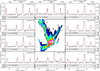 |
Fig. 3 Examples of NH3(1,1) spectra at ten positions in the cloud, plotted surrounding the H2 column density derived from the NH3 emission (discussed later in Sect. 3.2). The model fit is plotted over each spectrum in red, whilst the residual of the two is plotted in the bottom panel with the standard deviation quoted in mJy beam−1. Regions of specific interest include those where the velocity width is seen to increase (spectra 1 and 6), positions where the centroidvelocity changes as a filament meets the central hub (spectra 3, 4 and 7) and the large starless core MM2 (spectrum 8). It is clear that there is only a single velocity component everywhere in the cloud, with some lines being narrow enough to start resolving further hyperfine components (spectrum 10), and some showing the tell-tale signs of the cloud identified by Peretto et al. (2014) at a V sys = 54 kms−1 that likely overlaps in projection with the north-east filament (spectrum 1 and 2). |
3.1.2 Centroid velocity
The channel map of the main NH3(1,1) transition in this model cube is shown in Fig. A.1. It shows large-scale velocity structures, with filaments appearing at different velocities, with a total velocity span of ~7 km s−1, consistent with the global velocity structure observed in N2 H+(1–0) by Peretto et al. (2014). Figure 4 (middle columns) display the line of sight centroid velocity from both the NH3(1,1) and (2,2) transitions. As a result of the increased angular resolution (almost by an order of magnitude), we observe a far more complex velocity field in SDC13 than previously revealed by the IRAM 30 m data. In particular, we resolve both longitudinal and radial velocity gradients across all filaments (where filaments are named following the same convention as Peretto et al. 2014, and their extraction is discussed in Sect. 4.2). This is most evident across the bottom half of the north-east orientated filament, and across the entire south-east orientated filament (labelled in Figs. 4 and 5). At face value, it is not clear that our ammonia velocity map is consistent with the N2 H+(1–0) data published by Peretto et al. (2014). In order to check for consistency, we fitted the hyperfine components of the NH3(1,1) and NH3(2,2) emission from the GBT data only (see Appendix D), at a similar angular resolution to the IRAM 30 m data. The GBT velocity map reveals gradients along each and every filamentary arm towards the centre of the system, identical to those observed in the N2 H+(1–0) IRAM 30 m data. The large number of NH3(1,1) hyperfine components makes the best fit centroid velocity and velocity width both very accurate. We estimate that the related uncertainty is less than half a channel width, i.e. ~0.05 km s−1.
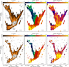 |
Fig. 4 Integrated intensity (first column), centroid velocity (middle column) and velocity width (right column) of the NH3 (1,1) transition (top row) and NH3(2,2) transition (bottom row). The NH3(1,1) data were masked to 5σ, while the weaker NH3(2,2) data were masked to 3σ. Filaments are named in the top left panel. Contours in the top left panel are in steps of 7 K × km s−1, from 5 K × km s−1 to 61 K × km s−1, while contours in the bottom left panel are in steps of 1 K × km s−1, from 1 K × km s−1 to 6 K × km s−1. Beam information is plotted in the bottom right corner of each panel, while the scale of 1 pc is plotted in each panel of the top row. |
3.1.3 Velocity width
Figure 4 (right column) shows the FWHM velocity width of the dense gas. We report an increased velocity width at the filament hub junction, peaking at ~1.6 km s−1, consistent with the broadening reported by Peretto et al. (2014). Interestingly, we also observe local increases of the velocity width sprinkled along each filamentary arms. As discussed later in Sect. 4, these are correlated to peaks in the H2 column density. We note that opacity broadening is accounted for as a consequence of the fitting procedure used. However, because of the relatively large peak NH3(1,1) main line opacity of 4.7, we independently performed a Gaussian fit of the optically thinner of the hyperfine components. By doing so, we observe the same increase of the line width. We conclude that the line widths plotted in Fig. 4 represent the true velocity dispersion of the dense gas. Furthermore, we also notice the velocity width increases around some localised regions at the edges of filaments, most evident on the Eastern edge of the lower portion of the north-east filament, and the western edge of the lower portion of the north-west filament.
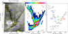 |
Fig. 5 Left: Spitzer 8 μm flux density in units of MJy sr−1, overlaid with IRAM 30m MAMBO 1.2 mm dust continuum contours in steps of 5 mJy beam−1, from 3 to 88 mJy beam−1. Crosses denote the positions of identified 1.2 mm MAMBO compact sources (white for starless and blue for proto-stellar, Peretto et al. 2014) and two 1.3 mm SMA continuum sources (in black crosses, McGuire et al. 2016). Middle: H2 column density map in units of 1022 cm−2, derived fromthe NH3 integrated intensity. Overlaid contours are placed in 1 × 1022 cm−2 steps, from 2 × 1022 cm−2 to 12 × 1022 cm−2. Right: extracted cores (black crosses, numbered according to Table 2) and filaments (labelled coloured lines). The extraction of these structures are discussed in Sect. 4. Extra cores at the outskirts of the north-east and south-east arms are in the more diffuse regions of the cloud where the spines did not extend through. Spine colours match those in subsequent figures. |
3.2 H2 column density map
Ammonia isoften called the thermometer of molecular clouds (e.g. Maret et al. 2009), as the temperature of the gas can be directly calculated from the ratio of the intensities of the two main lower metastable transitions, NH3(1,1) and NH3(2,2). In turn, the ammonia column density map can be calculated using the temperature, opacity and brightness temperature maps. The derivations of each of these quantities can be found in Appendix B. Using a constant abundance of ammonia with respect to H2 of 3 × 10⁻⁸ (Harju et al. 1993) one can then compute the H2 column density map of SDC13. This calculation is however limited by the weaker emission of the NH3(2,2) transition, which in our case traces 42% less of the cloud area than the NH3(1,1) transition. To overcome this, we take a median value of the temperature across the cloud of 12.7 K (the full temperature map and histogram are shown in Appendix B). The corresponding column density map is displayed in Fig. 5. Comparing this column density map to that calculated with a non-uniform temperature, we are satisfied that assuming a constant temperature across the entire cloud does not introduce any significant changes to the morphology of features in the map, whilst extending the coverage of the map (a result also reported by Morgan et al. 2013). Increasing the temperature by a standard deviation (1.8 K) decreases the column density by 12%. It is important to note that given our non-detection of the MM1 proto-stellar core, our assumption of constant abundance across the entire cloud (whilst a fair assumption given the excellent correlation between the NH3(1,1) integrated intensity and the 8 μm Spitzer emission) does not hold entirely for such portions of the cloud as the MM1 region. Deriving the H2 column density from the 1.2 mm dust continuum emission (presented in Peretto et al. 2014) and comparing it to the NH3 column density shows that the assumed abundance is consistent with the data, and has a dispersion of only ~3%. Overall, we take a conservative estimate of the uncertainty on the column density of 20%.
4 Analysis: structure extraction
In this section, we discuss the identification of cores and filaments within SDC13.
4.1 Cores
Dendrograms are a useful tool for the understanding of hierarchical structure and are invaluable for understanding the fragmentation of molecular clouds (e.g. Rosolowsky et al. 2008). We used the dendrogram code developed by Peretto & Fuller (2009) to extract all clumps from the NH3 derived H2 column density map at regular isocontours. A minimum isocontour value is set at N(H2) = 1 × 1022 cm−2 defining the“trunk” of the dendrogram tree, with a regular isocontour spacings at 1σ of 0.04 × 1022 cm−2 throughout, and a 5σ detection threshold. A pixel limit of seven defines the smallest size of structure considered resolved, as it roughly matches the beam shape. Cores were identified as the highest levels in the dendrogram hierarchy (termed “leaves”) meaning that they contain onlythemselves and no other sub-structures. All observed core properties are listed in Table 2, such as the central core co-ordinates, major and minor axes, position angle, aspect ratio, radius and mean H2 column density. Core radii were calculated by considering each isocontour core boundary a disc with an equivalent area. The smallest deconvolved core radius can be seen to match half of the beam width, a direct effect of matching the pixel limit of the extraction code to the beam.
We identified 28 cores, of which seven lie along each of the north-west and north-east filaments, three lie along the south-east filament and two along the north filament (plotted in the right panel of Fig. 5). The remaining cores mostly lie at the end of the north-east filament. Their starless (or proto-stellar) nature was identified by the lack (or presence) of Spitzer 8 and 24 μm sources. Only three proto-stellar sources were detected, which were already identified by (Peretto et al. 2014; listed in Table 2). Core masses were calculated by taking the mean H2 column density (middle panel of Fig. 5, calculated from the NH3 column density) within the core boundary, and setting the average molecular weight, μ = 2.8. Two mass estimates were calculated for each core, one excluding the outer column density shell (effectively excluding the “background”, equivalent to the “clipping” scheme of Rosolowsky et al. 2008) regarded as the lower limit of the mass, and one that incorporates the background column density (equivalent to the “bijection” scheme of Rosolowsky et al. 2008), regarded an upper limit of the mass. Small column density peaks on top of a large background column density will generate very different mass estimates. The cores we identify here range from low- to high-mass, with the most massive ones being located near the filament junctions (core IDs 26, 27 and 28 – see Fig. 5). Both mass ranges, as well as the virial ratio (see Sect. 5.5) are listed in Table 2. The association of the newly identified cores with those published in Peretto et al. (2014) is also provided in the table. The dominant source of uncertainties in the estimate of core properties are the distance (11%), the abundance (within a factor of two) and the way cores are defined (bijection versus clipping – see Table 2). We note that uncertainties related to distance and abundance are systematic and therefore will not change observed trends.
As already mentioned in Sect. 3.1.3, we do observe a correlation between the increase of velocity width and the presence of cores. In order to quantify the number of cores displaying such behaviour, we systematically computed the average velocity width within the extracted core area at its position in the dendrogram tree where it is first identified as a leaf (Δ V core). Doing so we find that 73% of the cores show an increase in their mean velocity width of ≥10% when compared to the velocity width of the underlying “branch” structure of the dendrogram tree (Δ V branch, as shown in Fig. 6). Furthermore, 87.5% of these belong to the starless core population (according to the lack of mid-infrared point source). To visually demonstrate this increase even further, we split the cores into two sub-samples. The first contains cores with Δ V core∕ΔV branch > 1, whilst the second contains cores with ΔV core∕ΔV branch ≤ 1.
In Fig. 7 we stack each of the sub-samples separately and take the mean velocity width (for starless cores only). The overplotted contours are of the average H2 column density. This figure clearly shows that the velocity dispersion is increased over the entire extent of the cores, with a peak towards their centres.
Observed and calculated properties of extracted cores.
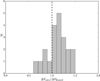 |
Fig. 6 Histogram of the ratio of the average velocity width within a core region (Δ V core) to that of the underlying branch structure (ΔV branch) in the dendrogram tree. The vertical dashed line indicates where ΔV core = ΔV branch. |
4.2 Filaments
The orientation and morphology of all filamentary structures were constrained by identifying the spines of the filaments. As the name suggests, the spine is considered the backbone of a filament, tracing the pixels where the column density exhibits a local maximum in at least one direction. This was quantified by computing the second derivative matrix (e.g. Schisano et al. 2014), that is the Hessian matrix, for each pixel in the column density map. Then, by diagonalising the matrix, and selecting areas where at least one of the eigenvalues is negative, we can identify the filament areas. To reduce this to a spine, we used the THIN IDL function. The local orientation of the filaments at each pixel along the spine is provided by the angle of the first eigenvector and the x axis of the image. Figure 5 shows the spines of each of the four identified filaments, and Table 3 compiles their properties. The masses of all filaments (including the portions of the spines that intersect the central hub) total to ~1000 M⊙, equal the mass quoted by Peretto et al. (2014). Separating the central hub region from the filaments places half the total mass in the hub region and half in the filaments.
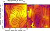 |
Fig. 7 Average stacked velocity width of cores identified with ΔV core∕ΔV branch > 1 (left) and those with ΔV core∕ΔV branch < 1 (right). Included in the construction of the left and right panels are 12 and 5 cores, respectively. Only starless cores within the filamentary arms are included, excluding both proto-stellar and central hub region sources. Contours are of the respective average stacked column density in 0.5 × 1022 cm−2 steps from 0 to 6 × 1022 cm−2 on the left, and in 0.4 × 1022 cm−2 steps from 0.2 to 3.8 × 1022 cm−2 on the right. |
4.2.1 Longitudinal filament profiles
We first study the filaments along their spines. Figure 8 plots the line profiles of all four filaments in H2 column density (first row), velocity width (second row) and absolute centroid line-of-sight velocity (third row) where the origin of the filaments was defined to reside at the centre of the hub. Filaments show variations in all quantities, and on a range of spatial scales. First, we notice that these variations are correlated in all three quantities, being particularly obvious for the north-east and north-west filaments. More specifically, core positions (marked by shaded regions on all panels) correlate with the velocity width, but also in centroid velocity where local velocity gradients are developed. This is shown in the fourth row of Fig. 8 where we plot the absolutevelocity gradient along the spine, evaluated over the mean core size of 0.1 pc. We note that a significant fraction of the cores (~63%) are located at a peak of velocity gradient. In the bottom row of Fig. 8 we plot the rotational temperature derived from the NH3 emission. Although quite variable along the length of the filament, we do not find a correlation between the temperature and core positions, nor the kinematic properties. We conduct Spearman’s rank correlation coefficient test on these correlations for all four filaments separately. We find a definite correlation between the column density and velocity width peaks in every filament (as shown in Fig. 9) with vanishingly small p-values in every filament with coefficients ranging from 0.24 in the north-east filament (indicating a moderate correlation), to 0.74–0.91 in the other three filaments (indicating a strong correlation). We find similarly small p-values in the column density and centroid velocity correlations, showing to us a definite link between all three of these properties. Furthermore, we notice that there are other common features to all filaments, such as the strongest column density and velocity dispersion peaks located at the origin of the filaments. Note that this is not true for the north-east filament, but would likely be true if the abundance of ammonia towards the MM1 proto-stellar core (Peretto et al. 2014 labelled in the left panel of Fig. 5) were not decreased (see Sect. 3.1.1). More generally, it is interesting to note thatsimilarities emerge in the large scale morphology of all profiles between pairs of filaments (the north-west and north-east filaments on one side, and the north and south-east filaments on the other). Overall, such similarities are suggestive of the common physical origin of the SDC13 filament evolution, as discussed in detail throughout Sect. 5.
Summary of filament properties.
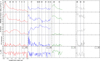 |
Fig. 8 Profiles along the spines, where each column denotes a different filament (north-west in red, north-east in blue, north in green and south-east in grey). The origin of each spine was centred at the hub region. The first row plots the column density of H2 calculated from the fitted NH3 integrated intensity. The second row plots the FWHM velocity width, while the third row plots the absolute centroid line-of-sight velocity (offset from the cloud systemic velocity of 37 km s−1), both also from the hyperfine structure fitting. The fourth row plots the absolute velocity gradient evaluated over the mean core size of ~0.1 pc. The fifth row plots the rotational temperature derived from the NH3 emission (see Appendix B.2) which has a standard deviation of 1.8 K. The drops of temperature below 8 K are artificial and due to missing NH3 (2,2) detections at these particular locations. The vertical shaded regions in each panel correspond to the peak N(H2) positions of the cores along the spine, and are ~0.1 pc wide. |
4.2.2 Radial filament profiles
To construct a radial view of the filaments, we interpolate along an 0.4 pc slice perpendicularly orientated to each spinal pixel using a Taylor expansion method (where the interpolation step is equivalent to half a pixel). Every slice is used to construct radial position-velocity (PV) profiles from the NH3 hyperfine structure fitted cube. Any prevailing velocity gradient orientated parallel to the filaments however causes each radial PV slice to be centred differently in velocity, effectively smearing the mean radial PV profile. This was corrected by aligning each PV slice to the central velocity of the slice.
It is clear from the on-axis concentric nature of the highest intensity emission in the north and north-west filaments in Fig. 10 that any radial velocity gradient does not dominate the velocity field. The intensity-weighted mean of these profiles doesappear flat at their centremost regions around the spinal pixel, with relatively low radial velocity gradients of 0.3 km s−1 pc−1 and 0.2 km s−1 pc−1, respectively.In contrast, the south-east and north-east filaments have rather significant mean radialvelocity components across their entire width, corresponding to 1.1 and 1.5 km s−1 pc−1, respectively.Although significant in this context, these gradients are not as strong as others observed by Fernández-López et al. (2014) or Beuther et al. (2015) for example, who observe radial gradients an order of magnitude larger than longitudinal velocity gradients in Serpens South and IRDC 18223, respectively. The radial variations of the velocity width are plotted in the bottom panels of Fig. 10. These profiles show that the longitudinally averaged velocity dispersion varies across all filaments, with, in some cases, local minima along the filament spine, and local maxima at the edges. However, as discussed in Sect. 4, these trends result from the average of a number of different processes that are mixed-up together in such profiles.
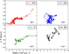 |
Fig. 9 Correlations of velocity width to H2 column density along the filament spine directions for the north-west (top left) north-east (top right), north (bottom left) and south-east (bottom right) filaments, excluding the portion of the spines that intersect the central hub regions (identified as where the filament can no longer be distinguished from the hub). Filled circles denote the spinal pixel position of the identified cores along the filaments. A mean error is plotted in the bottom right of each panel, equal to ±20% on the mean H2 column density, and ± 0.05 km s−1 on Δ V. |
4.3 JVLA/GBT combined versus JVLA-only datasets
In previous sections, results obtained from the combined JVLA/GBT dataset were presented. As already mentioned in Sect. 2.3, such a combined dataset is optimal to recover emission at all spatial scales. However, when trying to characterise the gas properties of the densest parts of the filaments (i.e. cores and filament spines) as we have done above, results can be affected by the contamination of the larger scale, more diffuse, foreground/background emission. The effect of this contamination would be to dilute the observational signatures one is trying to identify.
For that reason we redid some of the analysis presented in earlier sections using the JVLA-only dataset, which traces only the most compact/densest regions of the cloud. We particularly focus on the velocity dispersion variations along the filament spines and towards the cores. By fitting the hyperfine components of the JVLA-only NH3 emission, wefind that the increase of the velocity width at the core positions is even larger than in the combined data set. This is illustrated in Figs. 11 and 12, reproductions of Figs. 7 and 8 but of the JVLA-only data. From these figures, one can see that the JVLA-only velocity width towards the core centres is 1.5–2 times larger than that of the surroundings, compared to a 1.1–1.4 factor in the JVLA/GBT combined data. We also notice that in the JVLA-only data the remaining starless cores also display an increase of velocity width. This analysis strengthens our conclusions about the local increase of velocity dispersion towards the SDC13 starless cores.
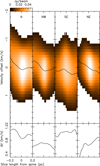 |
Fig. 10 Top:mean position-velocity diagrams across the north, north-west, south-east and north-east filaments (from left to right), where position denotes the length of a perpendicular slice relative to the central spine pixel in parsec, and the velocity are relative to the peak velocity of each slice. The overplotted black line shows the trend of the intensity-weighted mean offset velocity at each position along the radial slice. Mean radial gradients were computed within the inner 0.2 pc width around the spinal pixel. Bottom: mean variation in the velocity width in the radial direction, in km s−1. |
5 Discussion
In this section, we discuss the various observational properties of the filaments in SDC13 in terms of filament evolution theories. To facilitate the visualisation of the filament properties, the radial interpolation carried out in Sect. 4.2.2 was carried out on the column density, centroid velocity, velocity width and Spitzer 8 μm opacity for all filaments. Aligning each slice to the pixel that lies along the filament spines gives us a unique deprojected perspective of the filaments (Fig. 13) i.e. a view of the filament independent of their on-sky projection, making some of the filament features discussed below stand out.
 |
Fig. 11 Velocity width profiles of the north-west (red), north-east (blue), north (green) and south-east (grey) filaments in the combined data (top row, as presented in the second row of Fig. 8) and the JVLA-only data (bottom row), evaluated over the same filament spines as identified in Sect. 4.2. |
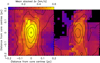 |
Fig. 12 Reproduction of Fig. 7, but for the JVLA-only data. The average stacked velocity width of cores identified with velocity width peaks (left) and those without peaks (right). Included in the construction of the left and right panels are 13 and 4 cores, respectively. Plot details are the same as those detailed in the caption of Fig. 7. |
5.1 Supercritical filaments
One important parameter of interstellar filaments regarding their stability is their mass-per-unit-length, Mline. The first step towards measuring this quantity is to determine their radial column density profiles. In our attempt to compute these profiles, neither a Gaussian distribution nor a Plummer profile (Whitworth & Ward-Thompson 2001) accurately reflects the complexity of the radial column density distributions (unlike Arzoumanian et al. 2011, for example, see Appendix E). Therefore, we instead integrate all radial column density distributions using the Trapezoidal rule at every position along the filaments spines to calculate the mass per unit length. A rough estimation of the filament widths were obtained by taking  times the standard deviation of the radial column density profiles. In calculating the mean Mline and filament widths (listed in Table 3), we excluded the regions that intersected the cloud hub (identified as belonging to the radial column density slices where the extended nature of the hub emission makes the determination of the width impractical). Figure 14 plots the evolution of the filament width and Mline along the filament lengths, respectively. The critical mass per unit length,
  (where a0 is the isothermal sound speed and G is the gravitational constant) is the critical value above which an interstellar filament becomes gravitationally unstable to radial contraction and fragmentation (Ostriker 1964). For a typical 10 K filament, Mline,crit = 16M⊙ pc
![$^{-1} \left[\frac{T}{10K}\right]$](/articles/aa/full_html/2018/05/aa31587-17/aa31587-17-eq3.png) . At the mean rotational temperature of SDC13 of 12.7 K, a0 = 0.21 km s−1 and the critical mass per unit length is 20.4 M⊙ pc−1. All SDC13 filaments can be classed as thermally supercritical (see Table 3) therefore prone to radial gravitational contraction and fragmentation along their lengths. When considering the effective sound speed,
. At the mean rotational temperature of SDC13 of 12.7 K, a0 = 0.21 km s−1 and the critical mass per unit length is 20.4 M⊙ pc−1. All SDC13 filaments can be classed as thermally supercritical (see Table 3) therefore prone to radial gravitational contraction and fragmentation along their lengths. When considering the effective sound speed,  km s−1 (where σNT,0 = 0.15 ± 0.02 km s−1, taken from Fig. 17 as the most representative value of the filament dense gas prior to fragmentation – see Sect. 5.4) the critical mass per unit length becomes 31.3 M⊙ pc−1, a factor of 1.5 larger than the previously calculated thermal Mline,crit, but still a factor of 4–10 lower than the measured filament line masses.
5.2 Core separation and age estimates
The separation of cores along filaments can provide indication on the physical mechanism driving the fragmentation. The top panel of Fig. 15 shows the Gaussian Kernel Density Estimation (KDE) plot of core separations in all filaments (excluding hub cores) where the two plotted distributions each use a different bandwidth Gaussian. The core separations were calculated on the original on-sky projected filament spines, and not from the deprojected plots in Fig. 13, although both provide identical results. There is clearly a peak in each distribution at a core separation λcore ≃ 0.37 ± 0.16 pc. Regular spacings in IRDCs with core separation ranging between ~0.2 and 0.4 pc have already been reported (Beuther et al. 2015; Henshaw et al. 2016; Zhang et al. 2009). For comparison, we simulated the four filaments by randomly placing the same number of cores as observed along each of the four filament lengths and calculated the separation of each consecutive core pair (e.g. Teixeira et al. 2016), and repeated the process 100 000 times. In doing this, we stipulated that the smallest core separation in these random core distributions must exceed the beam size, equivalent to 0.07 pc spatial scale. We can clearly see that the observed cumulative histogram (black) is steeper than the simulated cumulative histogram (red) in the bottom panel of Fig. 15. To quantify these differences, we used the Kolmogorov–Smirnov test to estimate the probability that these two histograms originate from the same parent distribution. We find that there is a 15% chance that this is the case, exceeding the significant test limit of 5%. However, coupled with the relatively large K-S statistic of 0.28 (suggesting a large maximum distance between the two cumulative distributions), we reject the null hypothesis and consider that these two histograms are significantly different, demonstrating that the core spacing in the SDC13 filaments are not randomly distributed. The median value of λcore in each filament is given in Table 3. Note that looking at the deprojected view of the filaments in Fig. 13, the spacing of the north-west filament seems to be more regular than the others. This is supported by the lower core spacing standard deviation of the north-west filament, i.e. 0.06 pc (whilst excluding core number 27 in the hub centre) versus 0.21 pc for the north-east filament.
Inutsuka & Miyama (1992) and Miyama et al. (1994) showed that filaments in hydrostatic equilibrium fragment under density perturbations whose wavelengths are four times the filament diameter. Looking at the relevant values given in Table 3 we see that the ratio between the core separation of the SDC13 filaments and their widths varies between 1.1 and 2.1 which, given the unknown inclination, is compatible with a ratio of 4. However, in a turbulent medium, filaments in equilibrium are likely to be rare objects. Interestingly, Clarke et al. (2016, 2017) studied the fragmentation of non-equilibrium, accreting filaments and showed that the fastest growing mode of density perturbations in such systems, λcore, is a function of the time it takes to build-up a critical filament through accretion, τcrit, and the effective sound speed, aeff,0:
 (1)
(1)
By measuring the core separation and the gas temperature, it then becomes possible to derive τcrit. One can also relate τcrit to the accretion rate onto the filament Ṁ by:
 (2)
(2)
where Mline,crit is the critical mass per unit length. Values for τcrit and Ṁ (derived using the previously calculated aeff,0 = 0.26 km s−1 and Mline,crit = 31.3 M⊙ pc−1) are given in Table 3 for each filament. According to this model, we see that it takes on average ~0.68 Myr to form the SDC13 filaments up to the critical mass per unit length, with an average accretion rate ~46.5 M⊙ pc−1 Myr−1. Interestingly, assuming that the derived accretion rate remained constant over the entire filament lifetime, one can derive the age, τage, through:
 (3)
(3)
As shown in Table 3 we obtain an average value of τage ~ 5.9 Myr, which implies that the elapsed time since the filaments became critical is ~5.2 Myr. Based on the observed longitudinal velocity gradients and assuming that the gas is free-falling, Peretto et al. (2014) estimated that the SDC13 filaments had been collapsing for ~1–4 Myr. This is consistent with the estimate based on the Clarke et al. (2016, 2017) model. However, in the calculation of τcrit we have not taken into account projection effects in the estimate of λcore. Doing so will increase τcrit by a factor 1∕ cos(θ) where θ is the angle between the direction of the main axis of the filament and the plane of the sky, which for an average angle of 67° (Peretto et al. 2014) is equal to 1.7 Myr. This brings the estimated age of the filament to 15.1 Myr, more than a factor of 3 larger than the dynamical timescale estimated by Peretto et al. (2014).
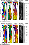 |
Fig. 13 Deprojected views of the north-west (top) and north-east (bottom) filaments. The filament length is plotted on the y-axis, while the length of the radial slices from the central spine pixel in plotted on the x-axis. In both sub-figures, the panels show (from left to right) the H2 column density derived from the NH3 emission, the line-of-sight velocity, the velocity width, the opacity derived from the 8 μm Spitzer emission, and finally the core ID as listed in Table 2. Contours in the first four panels are of the column density, from 1 × 1022 cm−2 to 11 × 1022 cm−2, spaced by 1 × 1022 cm−2. The plots for the south-east and north filaments are in Appendix C. |
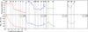 |
Fig. 14 Caption as for Fig. 8. First row: filament width calculated from 2.35 times the standard deviation of the radial column density distributions. The jump in width seen at roughly 1.2 pc in the north-west and north-east filaments is due to the exit of the filament spine from the hub. The mean filament width was evaluated beyond this point. Second row:mass per unit length, evaluated from conducting a Trapezoidal integration under all radial column density distributions. |
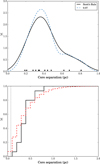 |
Fig. 15 Top:Gaussian Kernel Density Estimation (KDE) plot of the separation of each consecutive core pair in each of the four filaments. Each line denotes a different bandwidth Gaussian, 0.07 pc (equivalent to the beam size, in dashed blue) and 0.1 pc (derived by the standard Scott’s Rule, and equivalent to the mean core radius, in black). Black circles at N = 0.05 are overplotted to show the positions of the individual spacings in the sample. The standard deviation is 0.16 pc. Bottom: normalised, cumulative distribution of the observed core separation (black line) and the 100 000 simulated core separations (dashed red line). The bin size in both plots was set to be slightly larger than the beam at 0.1 pc in size. The verticaldotted line in both denotes the data spatial resolution of 0.07 pc, used as a cut-off of the allowed simulated spacings. |
5.3 Collapse timescales
With all the hierarchical structure in SDC13 extracted using the dendrogram method, we calculate their radii, aspect ratios and mean densities. As the free-fall collapse time of a structure depends only on the density, we calculate tff for all extracted structures, from the base of the dendrogram tree up to the leaves using:
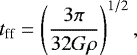 (4)
(4)
where G is the gravitational constant, and ρ is the density of the core (for which we use the upper limit on the mass in Col. 12 of Table 2). However, this is not an appropriate approach for non-spherical objects like the high-aspect ratio filamentary structures within SDC13 (Pon et al. 2012; Toalá et al. 2012). Clarke & Whitworth (2015) derive a collapse timescale (tcol) valid for both filamentary and near spherical structures:
 (5)
(5)
where Ao is the aspect ratio, valid down to values of Ao ≳ 2. The filamentary nature of SDC13 from large to small scale (i.e. 61% of cores having Ao > 2 – Table 2) justifies the need to use Eq. (5). Figure 16 shows the collapse time tcol for all identified structures in the SDC13 dendrogram. Overall we see a decrease of the collapse time, from ~0.7 to 0.1 Myr as we go from large to small structures as a result of the structures’ decreasing aspect ratios and increasing densities. A consequenceof this hierarchical collapse time is that cores will collapse well before the filaments. This is the basic idea behind the hierarchical star formation models of Vázquez-Semadeni et al. (2009, 2017). On the same figure, we see one structure in the north-east filament that departs from the rest of the SDC13 structures, with a longer collapse time than the structure in which it is embedded in. This is due to the particularly long aspect ratio of that particular structure. We also notice that the same structure exhibits the strongest radial velocity gradient (see Sect. 5.2) and the smallest core separation (see Table 3). As speculated later in the paper, we argue that this is a direct consequence of the compression of the pre-existing filament by the feedback of a nearby star formation event.
5.4 Linewidth as a probe of infall
The increase of velocity width within the cores can be quantitatively compared to the velocity dispersion within the filaments. In that respect, we calculated the non-thermal contribution of each pixel within SDC13 following (Myers 1983):
 (6)
(6)
where ΔV obs is the fitted FWHM velocity width, kb is the Boltzmann constant, and  is the mass of an NH3 molecule. To determine whether the filaments are subsonic or supersonic in nature, we compare this non-thermal sigma velocity dispersion to the isothermal sound speed a0 at 12.7 K of 0.21 km s−1. Figure 17 shows the histograms of σNT∕a0 for all four filaments, where pixels within core regions only are overplotted in white. Overplotted in black are the corresponding distributions taken from the JVLA-only data. We see that in all filaments the gas in the combined data is predominantly supersonic, however, the north-west and north-east filaments also peaks significantly in the sub- and/or transonic regime. This second peak is coincident with that of the JVLA data which only exhibits a minor supersonic tail in its distribution whilst peaking sub- and/or transonically.
Barranco & Goodman (1998) and Goodman et al. (1998) find that σNT remains constant across core regions, and increases once outside the core boundary. They call this behaviour velocity “coherence”, suggesting that cores have sizes that are intimately linked to the turbulence properties. We observe a different behaviour, with 88% of pixels within core regions have σNT∕a0 ≥ 1. This is consistent with our systematic identification of 73% of cores exhibiting a peak in velocity width. However, 87% of pixels within the surrounding filament also have σNT∕a0 ≥ 1. Despite this similarity in the core and filament pixel distributions, conducting a Kolmogorov–Smirnov test of the two show vanishingly small p-values with moderate coefficient values (between 0.2 and 0.3), indicating they are significantly different. In the JVLA data however, 55% of pixels within core regions peak supersonically compared to only 36% of filament pixels. This furtherdemonstrates that with the addition of the extended background emission in the combined data, the kinematics of the cores have become diluted and similar to that of the surrounding filament. Probing the densest gas with the JVLA-only shows that the kinematics of the cores are more distinct from the surrounding filament.
A decrease of velocity dispersion towards low-mass pre-stellar cores has been previously observed (Fuller & Myers 1992; Goodman et al. 1998; Caselli et al. 2002; Pineda et al. 2010, 2015). More recently, this transition to coherence has also been observed towards entire, parsec-long filaments (Hacar & Tafalla 2011; Hacar et al. 2016). Transonic cores and filaments are expected to form in a turbulent ISM where supersonic shocks generate stagnation regions where turbulent energy has been dissipated (Padoan et al. 2001; Klessen et al. 2005; Federrath et al. 2016). In SDC13, with mostly transonic velocity dispersion (where both the combined and JVLA data sets peak in Fig. 17, hence best representing the dense gas of the system), everything indicates that the filaments represent such post-shock regions, the increase of the dispersion in some localised region at the edge of the filament being reminiscent of what Klessen et al. (2005) sees in their turbulent simulation of core formation. In this context, the velocity dispersion increase towards the core would be then purely generated by gravity (e.g. Ballesteros-Paredes et al. 2017).
Another possible explanation for a local increase of velocity dispersion towards the cores could be the presence of embedded proto-stellar sources. Even though we do not see any mid-infrared sources towards them, such protostars could be embedded enough to remain undetectable with both Spitzer and Herschel. These protostars could have associated outflows which disrupt the surrounding gas, contributing to a local increase in the velocity dispersion (Duarte-Cabral et al. 2012). ALMA observations of SDC13 cores at sub-arcsecond resolution could settle this issue.
 |
Fig. 16 Map where the outline of all extracted structures are coloured by their collapse timescale tcol in Myr. |
 |
Fig. 17 Non-thermal contribution to the velocity dispersions, divided by the isothermal sound speed at the temperature of the NH3 gas of 12.7 K i.e. the Mach number. The red histogram is the north-west filament, blue is the north-east, green is the north while grey is the south-east. The vertical dashed line denotes the transition from subsonic to supersonic motions. Overplotted in white in each panel is the Mach number of the core regions only from the combined data. The overplotted black line is the distribution of the JVLA-only velocity dispersion results. |
5.5 Evolution of the virial ratio from large to small scale
Using the dendrogram tree, we can estimate the virial ratio for all extracted structures. Following Bertoldi & McKee (1992), the virial ratio of a uniform density sphere is given by:
 (7)
(7)
where R is the radius and M is the mass of the cores found by the extraction code, respectively, and aeff is the total velocity dispersion considering both thermal and non-thermal contributions from all molecules. We use the upper limit on the mass as it matches the amount of gas responsible for the observed velocity dispersion. In the absence of significant magnetic energy density, structures with αvir < 2 are thought to be gravitationally bound, those with αvir ~ 1 are compatible with hydrostatic equilibrium, those with αvir < 1 are likely to be gravitationally unstable, while structures with αvir > 2 are unbound and either dispersing or held together by external pressure. Figure 18 shows the map of virial ratios for all SDC13 structures. Based on this map, it is clear that as we go from large to small scale, the virial ratio increases from αvir ~ 0.1 towards 1. Such low-values suggest that SDC13 is gravitationally unstable on all scales, and that the transfer of gravitational to kinetic energy could be the process responsible for the increase of the virial ratios on small scales.
Such an evolution of the viral ratio can be analytically described by the following equation:
 (8)
(8)
where Ek and Eg are the kinetic and gravitational energies, respectively, the 0 index indicates the initial value, i.e. at the start of the collapse/fragmentation, and ϵ is the fraction of the gravitational energy which is converted into kinetic energy. Note that as |Eg | becomes increasingly larger during the collapse, ϵ = 1 translates into αvir → 2, which is expected if all the gravitational energy were to be converted into kinetic energy. A mean aeff,0 ~ 0.26 ± 0.02 km s−1 is evaluated from Fig. 17 (as discussed in Sect. 5.1). By estimating each energy term of Eq. (8) for every core showing an increase of velocity dispersion one can determine which value of ϵ is required to reproduce the observed αvir value. Assuming that the cores of initial diameter λcore result from the fragmentation of a uniform density transonic filament of initial velocity dispersion aeff,0, one can rewrite Eq. (8) as:
 (9)
(9)
where  is a factor depending on the power law index kρ of the density profile of thecollapsing core, and β0 is its initial value before the onset of collapse (see Appendix F for a more detailed derivation). For simplicity, we assumed an initially flat density profile (i.e. β0 = 3∕5), and kρ = 2 once collapse begins (i.e. β =1). Figure 19 plots the energy conversion efficiency ϵ against the virial ratio for every core for both the combined JVLA/GBT data and JVLA-only data. On this plot, only starless cores are included, as proto-stellar cores, or cores at filament junctions are subject to extra energy sources that will affect the estimate of ϵ. One can see that a conversion efficiency between 20 and 50% can explain most of the observed velocity dispersion increases towards starless cores. The JVLA-only data points (orange circles), believed to be less contaminated by foreground/background emission to the cores, are clustered around a median efficiency of 35%.
Klessen & Hennebelle (2010) proposed a theory according to which accretion is capable of driving turbulent motions in galaxies on all scales, finding an ϵ value of a few percent when considering both galaxy and molecular cloud sized structures. Clarke et al. (2017) evaluate the efficiency required to reproduce a given velocity dispersion due to accretion driven turbulence in filament structures. They find an ϵ = 5–10% is sufficient to drive a σ1D ~ 0.23 km s−1, a consistent efficiency to that found by Heitsch (2013). While these are theoretical estimates, our observationally derived value of ~35% is somewhat larger. This could point towards an even more important role of gravity-driven turbulence than previously thought (see also Traficante et al. 2018; Ballesteros-Paredes et al. 2017).
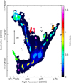 |
Fig. 18 Virial ratio map of all identified dendrogram structures. |
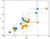 |
Fig. 19 Observed virial ratio plotted against the energy conversion efficiency of gravitational energy into kinetic energy for the combined JVLA/GBT data (in blue), and the JVLA-only data (in orange). Only starless along the filaments are plotted, as proto-stellar or hub centre cores are subject to extra energy source that will effect the estimate of ϵ. Errors were propagated using a Monte Carlo error propagation method. |
5.6 Origin of the radial velocity gradients
Two of the four SDC13 filaments exhibit strong radial velocity gradients, the largest of which in the combined data set reaches 1.5 km s−1 pc−1, an order of magnitude larger than in the remaining two filaments. In the JVLA-only data, although the morphology of the centroid line-of-sight velocity is the same as in the combined data, the magnitude of the radial velocity gradients double, approaching ~3.0 km s−1 pc−1 in both the north-east and south-east filaments. The physical origin of such gradients is unclear as they could be the result of accretion/compression, rotation, shear, or a combination of these. It is important to realise that, given the measured velocity gradients (up to 3.0 km s−1 pc−1), the crossing time of the filaments is ~0.3–0.4 Myr, which is a factor of ~3 lower than the estimated age of the filaments. This implies that, whatever the origin of the gradient is, it cannot be of disruptive nature or the filaments would already have dispersed. This therefore excludes shear motions as a possible origin. Here, we are going to investigate if the magnitude of the gradients are compatible with gravity and/or rotation.
For gravity to be responsible for radial velocity gradients in filaments, large-scale accretion into a plane is the only option as axisymmetric accretion would not produce any velocity gradients. Assuming that the filaments are infinitely long, then one can estimate the acceleration of a piece of gas at a radius r (Palmeirim et al. 2013), as:
 (10)
(10)
Substituting for the mean observed Mline of SDC13 we may calculate the rinitial that would produce the observed velocity (~0.3 km s−1) at a distance of 0.20 pc from the spine of the filament. By doing so we obtain rinitial ≃ 0.21 pc. The associated dynamical timescale is 3.3 × 10⁴ yr, nearly two orders of magnitude shorter than our age estimates for the filaments. This suggests that gravity alone is not the origin of the observed radial velocity gradients in SDC13. As proposed by Arzoumanian et al. (2013), turbulence generated by the accretion of matter onto filaments can provide an additional kinetic pressure that can eventually counteract the pull of gravity, and slow down the filament radial contraction, even though such a process might not be efficient enough (Seifried & Walch 2015). Magnetic fields can also contribute to slow down radial contraction, either when they run parallel to the main axis of filaments (Seifried & Walch 2015), or when in a helical configuration (Fiege & Pudritz 2000). However, B fields are often observed to be perpendicular to the main axis of the star-forming filaments (e.g. Palmeirim et al. 2013; Cox et al. 2016), therefore leaving the radial contraction unaffected.
We now investigate whether rotation could explain these observed gradients. Recchi et al. (2014) simulate the rotation about the main axis of filaments in equilibrium. They predict the radial velocity gradient required for rotation to stabilise filaments with varying Mline and temperature profiles against gravitational instabilities. Following their calculations for a mean SDC13 filament mass of 319 M⊙, mean filament length and width of 2.11 and 0.26 pc, respectively (hence central density of 4.8 × 10⁻¹⁷ kg m−3), and uniformtemperature profile (given we assume a constant temperature everywhere), a radial velocity gradient of 1.42 km s−1 pc−1 is required for rotation to halt the fragmentation of SDC13. Despite this being larger than the mean radial velocity gradient across the south-east filament (and less than that across the north-east filament) it is clear from the core extraction that there is indeed fragmentation along both filaments. Hence, we conclude that the observed radial velocity gradient cannot be solely due to rotation as the fragmentation was not halted. The model also only considers equilibrium filaments, which seems to be an unrealistic assumption to make for such a dynamic system as SDC13.
Therefore, we believe that the most likely origin for the observed radial velocity gradients is compression. We speculate that an external site of active star formation, clearly seen in Fig. 1 within 1 pc proximity to the north-east filament on the sky (centred on 18:14:33.5–17:33:30.0) may be compressing the north-east and south-east filaments of SDC13, influencing the radial velocity field and their density structures. The WISE catalogue ofHII region sources (Anderson et al. 2014) reveals a HII region they term as being radio-quiet (called G013.170−00.097) coinciding with this external star formation site, however there is no kinematic information available. Further to this, large scale 13 CO(1–0) and C18 O(1–0) emission from the IRAM 30 m telescope seem to show a cavity in emission corresponding to this region (Williams et al., in prep.), consistent with the clearing of material due to feedback effects. We find no maser emission such as water (Walsh et al. 2008; Purcell et al. 2012) nor methanol (Breen et al. 2012) around the position of the HII region. Other works have shown the influence of external feedback on the density structure of star-forming filaments (Peretto et al. 2012; Tremblin et al. 2014).
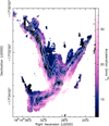 |
Fig. 20 Map of gravitational acceleration in SDC13 in units of 1× 10⁻¹² km s−2. Mass was calculated from the H2 column density map in the middle panel of Fig. 5. Contours are of the H2 column density in Fig. 5, plotted in 1 × 1022 cm−2 steps, from 2 × 1022 cm−2 to 12 × 1022 cm−2. |
 |
Fig. 21 Profiles along the spines, where each column denotes a different filamentary arm, as labelled (north-west in red, north-east in blue, north in green and south-east in grey). The origin of each of the spines was defined to begin at the heart of the hub. First row: acceleration due to gravity in SDC13 where the mass was calculated using the H2 column density map, while a uniform, mean cloud mass was used for the acceleration in the second row. Third row: absolute gradient of the acceleration from row three evaluated at each position over the mean core size of ~0.1 pc. The vertical shaded regions correspond to the positions of the cores along each of the filaments, are ~0.1 pc wide and overplotted by the core ID number in Table 2. |
5.7 Origin of the longitudinal velocity gradients
As mentioned in Sect. 4.2.1, the SDC13 filaments exhibit a complex oscillating longitudinal velocity profile which is at least partially correlated to their column density structure. In their simulations of turbulent cloud evolution, Smith et al. (2016) find very similar looking filament velocity profiles (see their Fig. 6). However, they argue that they do not see any clear correlation between the velocity fluctuations and the location of density peaks, concluding that the velocity fluctuations are the result of transient motions generated by the turbulent field in which the filaments are immerged. While we might be partly witnessing such effect in some of the SDC13 filaments, we do observe that ~63% of the SDC13 cores are located at a peak of velocity gradient as expected for cores accreting from their parent filaments.
One specificity of SDC13 is its hub morphology, suggestive of converging gravity-driven flows towards the filament junction. In order to evaluate if the hub morphology has an impact on the density and velocity profiles of SDC13, for each position we computed the amplitude of the acceleration following:
 (11)
(11)
where indices i and j correspond to given pixels in our SDC13 column density map, mi is the gas mass at pixel i, and ri,j is the distance between pixels i and j. Observationally, one only has access to the 2D projected quantities, and acceleration estimated that way can only provide trend indications and order of magnitude estimates. Figure 20 shows the acceleration map obtained from the SDC13 H2 column density map. As expected, the accelerations along the filament spine are at a minimum due to the axisymmetric nature of gravity in such systems. The acceleration appears to peak around the filament hub junctions and the edges of some filaments, reminiscent of the behaviour seen in the velocity dispersion map in Fig. 4. More interestingly, we have constructed acceleration profiles along each filament. These are shown in the first row of Fig. 21. We observe oscillations of the acceleration and an increase of the acceleration towards the hub centre which are reminiscent of the velocity structure. In order to check if this behaviour is due to the presence of cores or to the hub morphology, we constructed another acceleration map with uniform column density, effectively removing the presence of density fluctuations. The second row of Fig. 21 shows such profiles. One can see that, for the two main filaments (north-east and north-west), the acceleration profiles remain mostly unchanged, demonstrating that the hub morphology is the main driver of the acceleration fluctuation we observed, and therefore the driver of the SDC13 kinematics as a whole. Another interesting point is given by the last row of Fig. 21 where the gradients of the acceleration is provided. We notice here that the strongest acceleration gradient peak is associated with the most massive core within SDC13. Gradients of acceleration represent accumulation points and are therefore privileged locations for the formation of massive cores. The systematic presence of massive cores near the hub centre could therefore be a direct consequence of large acceleration gradients generated by the hub morphology.
6 Summary and conclusions
We have conducted a study of the SDC13 infrared dark hub filament system using the rotation inversion transition of NH3(1,1) and NH3(2,2). The fitting of the hyperfine structure of these lines allowed the construction of centroid velocity, velocity dispersion and H2 column density maps. These maps were used to identify both core structures and filament spines, allowing us to characterise their kinematics. We find that all filaments are supercritical, with an average transonic non-thermal velocity dispersion, and that core spacing is typically regular along them (~0.37 ± 0.16 pc). Using semi-analytical models of non-equilibrium filaments (Clarke et al. 2016, 2017) we determine that the filaments are a few Myr old, consistent with the SDC13 dynamical timescale derived by Peretto et al. (2014). We find that the large radial velocity gradients across two of the four filament cannot be due to gravity nor rotation, but most likely due to the compression caused by a nearby HII region. We also find that the velocity dispersion increases towards 73% of the identified cores, which we interpret as the result of the accumulation of matter due to the filament fragmentation process itself. We derive an average gravitational to kinetic energy conversion efficiency within these cores of ϵ ≃ 35%, larger than theoretical values published in the literature. Finally, we propose that the presence of massive cores near the filament junction is due to the large acceleration gradients produced by the hub morphology.
All elements put together, we propose a scenario for the evolution of the SDC13 hub-filament system in which filaments first form as post-shock structures in a supersonic turbulent flow. As a result of the turbulent energy dissipation in the shock, the dense gas within the filaments is initially mostly sub-sonic. Then gravity takes over and starts shaping the evolution of the hub, both fragmenting filaments and pulling the gas towards the centre of the gravitational well. By doing so, gravitational energy is converted into kinetic energy in both local (cores) and global (hub centre) potential well minima, generating more massive cores at the hub centre as a result of larger acceleration gradients.
Acknowledgements
GMW gratefully acknowledges the support of an STFC postgraduate studentship. NP wishes to acknowledgesupport from STFC under grant number ST/N000706/1 and ST/M000893/1. We thank the anonymous referee whose report helped improve the quality of this paper. This research made use of APLpy, an open-source plotting package for Python hosted at http://aplpy.github.com.
Appendix A Channel map
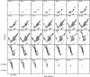 |
Fig. A.1 Channel map of the main transition of NH3(1,1) in the model combined data cube. Contour levels are placed at 0.05 Jy beam−1 steps, from 0.05 Jy beam−1 to 0.2 Jy beam−1. The channel velocity in km s−1 is plotted inthe top left corner of each panel. Right Ascension and Declination are in the J2000 epoch. |
Here we show the channel map of the main NH3(1,1) emission in SDC13.
Appendix B Opacity, temperature and column density
Here we present a more in depth discussion on the calculation of the opacity, temperature and column density directly from the relative intensities of the NH3(1,1) and NH3(2,2) lines.
B.1 Opacity
The optical depth defines the extent to which the NH3 gas is opaque or transparent, and was solved numerically (Barrett et al. 1977),
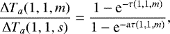 (B.1)
(B.1)
where the parameters ΔTa(1, 1, m) and Δ Ta(1, 1, s) refer to the observed peak spectra of the NH3(1,1) main (denoted by the m) and satellite (denoted by the s) components, which we take from the model hyperfine structure fit. The
expected relative intensities between the main and inner satellite lines is denoted by a. The opacity of the main NH3(1,1) line is denoted by τ(1, 1, m). This opacity is converted to the total opacity, τ(1, 1, t), by dividing by the relative strength of 0.502 (Li et al. 2003).
The opacity of NH3(2,2) is calculated similarly (Barrett et al. 1977),
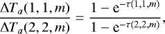 (B.2)
(B.2)
where ΔTa(2, 2, m) and τ(2, 2, m) are the observed peak of the spectra and the opacity of the NH3(2,2) main component, respectively. This opacity is converted to the total opacity, τ(2, 2, t) of NH3(2,2) by dividing by the relative strength of 0.796 (Li et al. 2003).
B.2 Temperature
The rotational temperature, which describes the relative populations of the NH3(1,1) and NH3(2,2) levels, was found using the following equation (Ungerechts et al. 1986),
![\begin{equation*} T_{\textrm{rot}} = - {T_{0}} \,/\, \mathrm{ln} \left( \frac{9}{20} \frac{\tau(2,2,t)}{\tau(1,1,t)} \left[ \frac{{\mathrm{\Delta}} v_{2,2}}{{\mathrm{\Delta}} v_{1,1}} \right] \right),\end{equation*}](/articles/aa/full_html/2018/05/aa31587-17/aa31587-17-eq20.png) (B.3)
(B.3)
where τ(2, 2, t) and τ(1, 1, t) are the total optical depths, and Δv2,2 and Δ v1,1 are the velocity widths of the NH3(2,2) and NH3(1,1) lines, respectively, and T0 = (E2,2 −E1,1)∕k = 41 K, where E1,1 and E2,2 are the energies of the NH3(1,1) and NH3(2,2) lines, respectively. The resulting Trot map is shown in the top panel of Fig. B.1, with its corresponding histogram in the bottom panel. We find no correlation between temperature and core positions, and only notice a very mild warming of material at the filament hub junctions.
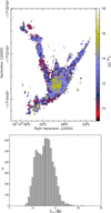 |
Fig. B.1 Top: map of the rotational temperature calculated using Eq. (B.3). It is clear that the coverage of the image is limited to that of the weaker NH3 (2,2) line. No correlation is found between temperature and core position. Bottom: histogram of the Trot map in the top panel. Vertical dashed line indicates the median value of 12.7 K. The standard deviation is 1.8 K. |
As outlined in Sect. 3.1.1, the NH3(2,2) emission is approximately 6 times weaker than that of NH3(1,1), resulting in 42% less coverage in the NH3(2,2) maps, and hence, the temperature maps. This limits the calculation of the column density of the cloud to this lesser coverage. To overcome this hindrance, we took a median Trot across the entire cloud of 12.7 K (e.g. Morgan et al. 2013). We discounted using the full temperature map whilst setting the median in the NH3(1,1) regions of emission only, as this caused edge effects in the resulting column density.
B.3 Column density
With opacity and temperature, we calculated the total column density of NH3 and H2. Firstly, the column density of the NH3(1,1) upper level only was calculated (Goldsmith & Langer 1999),
![\begin{equation*} N[\mathrm{NH}_{3}(1,1)] = \frac{8{k\pi}\nu^{2}_{1,1}}{{A}_{\mathrm{u,l}}{hc}^{3}} \int_{-\infty}^{\infty}T_{b}\mathrm{d}v\left ( \frac{\tau(1,1,t)}{1-\textrm{e}^{-\tau(1,1,t)}} \right ),\end{equation*}](/articles/aa/full_html/2018/05/aa31587-17/aa31587-17-eq21.png) (B.4)
(B.4)
where k is the Boltzmann’s constant, ν1,1 is the rest frequency of the NH3(1,1) line, Aul is the Einstein Coefficient for spontaneous emission, h is the Planck constant, c is the speed of light, τ(1, 1, t) is the total opacity of the NH3(1,1) line, and  dv is the integrated intensity of NH3(1,1) in Fig. 4a. Beam information has been cancelled out under the assumption that the source fills the beam.
Assuming local thermodynamic equilibrium (LTE), where the rotational temperature is assumed to equal the excitation temperature, we converted N[NH3(1, 1)] into the total column density of Ammonia, N(NH3), using (Goldsmith & Langer 1999),
![\begin{equation*} N(\mathrm{NH}_{3}) =\frac{N[\mathrm{NH}_{3}(1,1)]}{g_{1,1}} \textrm{e}^{E_{1,1}/{{k}T_{\textrm{rot}}}}Q(T_{\textrm{rot}}),\end{equation*}](/articles/aa/full_html/2018/05/aa31587-17/aa31587-17-eq23.png) (B.5)
(B.5)
where g1,1 is the statistical weight, E1,1 is the energy of the NH3(1,1) line, k is the Boltzmann constant, Trot is the rotational temperature, and Q(Trot) is the partition function. Expanding the partition function, Q(Trot) = ∑ igie−Ei∕kTrot over J and K energy levels, where J and K are the transition quantum numbers (Ungerechts et al. 1986),
![\begin{equation*} N(\mathrm{NH}_{3}) = N[\mathrm{NH}_{3}(1,1)]\left [ \frac{1}{3}\textrm{e}^{+23.26/T_{\textrm{rot}}}+1+\frac{5}{3}\textrm{e}^{-41.18/T_{\textrm{rot}}}\cdots \right ],\end{equation*}](/articles/aa/full_html/2018/05/aa31587-17/aa31587-17-eq24.png) (B.6)
(B.6)
where Trot is the median rotational temperatureof 12.7 K, and N[NH3(1, 1)] follows fromEq. (B.4).
We calculated the H2 column density by converting from NH3 using an abundance of [NH3]/[H2] ~ 3 × 10⁻⁸ (Harju et al. 1993). The final H2 column density map is shown in Fig. 5b.
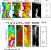 |
Fig. B.2 Deprojected views of the south-east (top) and north (bottom) filaments. The north filament was restricted to 0.2 pc either side of the spine due to contamination from the north-west and north-east filaments. The filament length is plotted on the y-axis, while the length of the radial slices from the central spine pixel in plotted on the x-axis. In both sub-figures (from the left), the first panel shows the H2 column density in units of 1022 cm−2, the second panel shows the line-of-sight velocity in km s−1, the third panel shows the velocity width in km s−1, the fourth panel shows the opacity derived from the 8 μm Spitzer emission, whilst the final panel labels the ID number of the identified cores. Contours in each panel are of the column density, from 1 × 1022 cm−2 to 11 × 1022 cm−2, spaced by 1 × 1022 cm−2. |
Appendix C Deprojected filaments
In Fig. B.2 we show the deprojected views of the south-east and north filaments (in the top and bottom panels, respectively). It is clear that there are radial velocity gradients present in both, stronger in the
south-east.
Appendix D GBT data
In Fig. D.1 we show the NH3(1,1) and NH3(2,2) integrated intensity, centroid line-of-sight velocity and velocity width of the GBT data.
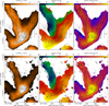 |
Fig. D.1 Integrated intensity (first column), centroid velocity (middle column) and velocity dispersion (right column) of the NH3 (1,1) transition (top row) and NH3(2,2) transition (bottom row) of the GBT data. The data has been regridded to the JVLA pixel size. The NH3 (1,1) data was masked to 3σ, while the weaker NH3(2,2) data was masked to 2σ. Contours in the top row correspond to the integrated intensity of the combined JVLA and GBT NH3 (1,1) data in stepsof 0.04 Jy beam−1 × km s−1, from 0.05 Jy beam−1 × km s−1 to 0.29 Jy beam−1 × km s−1, while contours in the bottom row correspond to the integrated intensity of the combined NH3 (2,2) data in stepsof 0.008 Jy beam−1 × km s−1, from 0.008 Jy beam−1 × km s−1 to 0.096 Jy beam−1 × km s−1. Beam information is plotted in the bottom right corner of each panel, while the scale of 1 pc is plotted in each panel of the top row. |
Appendix E Characterising radial column density profiles
To characterise the SDC13 filaments, we proceeded to fit each radial column density slice (found in Fig. 13) with Gaussian and Plummer (Whitworth & Ward-Thompson 2001) profiles, and intended to find the function that best described the observed structure. Examples of such fits are shown in Fig. E.1. Looking at the mean profiles of the north-east and north-west filaments (the fourth panels of Fig. E.1), it is clear that they are not well described by neither Plummer nor Gaussian fits. This trend continues when considering individual column density slices along the filaments (shown in the first three panels of Fig. E.1). Although a Plummer may reasonably well describe slice 50 in the north-west filament (and perhaps even the centre-most portion of slice 54 in the north-east filament) the extended emission in the majority of slices renders fitting them with Gaussian or
Plummer profiles inappropriate. We have evaluated further the impact of constraining the Gaussian fit parameters on the goodness of the fit itself. While setting the peak position of the Gaussian profiles to lie on the spine (i.e. x = 0) does not improve the produced fits, restricting the fitting to the inner portion of the filaments does result in better Gaussian fits of the central portion of the filament. However, filament properties (width and line mass) derived from such fits are very much dependent on the exact fitting range used. Such properties calculated from Trapezoidal integration of the asymmetrical profiles (as shown in Table 3 and Fig. 14) are less affected by such restrictions, and therefore more robust. Characterising filaments is fraught with difficulty, and caution must be observed whilst deriving global properties from their mean profiles (e.g. Panopoulou et al. 2017).
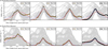 |
Fig. E.1 Results of fitting Gaussian (red line) and Plummer (blue dashed line) profiles to individual radial column density slices (orange circles in the first, second and third panels of each row) and the mean radial column density profile (black circles in the fourth panel of each row) of (a) the north-east filament (top row) and (b) the north-west filament (bottom row). The grey points in the background of each panel plots all of the radial column density slices simultaneously. Plummer profiles may on occasion well describe the inner regions of the filaments only, whilst Gaussian profiles fail to fit any of the distributions. Gaussian profiles are only found to reasonably fit some of the data once the fitting range is restricted tothe inner portion of the filament. |
Appendix F Derivation of the analytical expression of the virial ratio
Consider a uniform density filament fragmenting at the length scale equal to the separation of a core, λcore. In an idealised scenario, energy is conserved during collapse whilst fragmentation is happening. However, there is a fraction of energy converted from gravitational potential energy (Eg) into kinetic energy (Ek) at the time the filament fragmentation starts. This conversion may be expressed in the virial equation as an efficiency ϵ, where if no energy is converted,ϵ = 0. If energy conversion does occur, this can be expressed as a fractional increase in Ek, expressed as Ek = Ek,0 + ΔEk, where Ek,0 is the initial kinetic energy of the fragmenting core before collapse. This fractional increase in kinetic energy can be expressed as 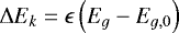 , where Eg,0 is the initial gravitational potential energy. Substitution into the standard virial ratio of αvir = 2Ek∕Eg gives:
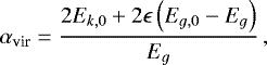 (F.1)
(F.1)
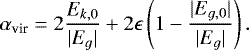
The energy terms may be expressed as:
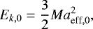 (F.3)
(F.3)
where aeff,0 is the 1D velocity dispersion, and:
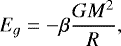 (F.4)
(F.4)
where  is a factor depending on the power law index kρ of the density profile of collapsing cores, and:
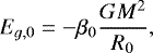 (F.5)
(F.5)
where β0 and R0 are the initial values of β and R before the onset of collapse. Making these substitutions gives:
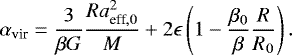 (F.6)
(F.6)
One may rewrite Ro as λcore∕2 under the assumption that all cores are initially their separation in size, and β0 = 3∕5 under the assumption that the filament is initially uniform in density (i.e. kρ = 0) before the onset of collapse. Making these assumptions simplifies the equation to:
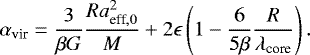 (F.7)
(F.7)
References
- Anderson, L. D., Bania, T. M., Balser, D. S., et al. 2014, ApJS, 212, 1 [NASA ADS] [CrossRef] [Google Scholar]
- André, P., Men’shchikov, A., Bontemps, S., et al. 2010, A&A, 518, L102 [NASA ADS] [CrossRef] [EDP Sciences] [Google Scholar]
- Arzoumanian, D., André, P., Didelon, P., et al. 2011, A&A, 529, L6 [Google Scholar]
- Arzoumanian, D., André, P., Peretto, N., & Könyves, V. 2013, A&A, 553, A119 [NASA ADS] [CrossRef] [EDP Sciences] [Google Scholar]
- Ballesteros-Paredes, J., Vázquez-Semadeni, E., Palau, A., & Klessen, R. S. 2017, MNRAS, submitted [arXiv:1710.07384] [Google Scholar]
- Barranco, J. A., & Goodman, A. A. 1998, ApJ, 504, 207 [NASA ADS] [CrossRef] [Google Scholar]
- Barrett, A. H., Ho, P. T. P., & Myers, P. C. 1977, ApJ, 211, L39 [NASA ADS] [CrossRef] [Google Scholar]
- Bergin, E. A.,& Langer, W. D. 1997, ApJ, 486, 316 [NASA ADS] [CrossRef] [Google Scholar]
- Bertoldi, F., & McKee, C. F. 1992, ApJ, 395, 140 [NASA ADS] [CrossRef] [Google Scholar]
- Beuther, H., & Steinacker, J. 2007, ApJ, 656, L85 [NASA ADS] [CrossRef] [Google Scholar]
- Beuther, H., Ragan, S. E., Johnston, K., et al. 2015, A&A, 584, A67 [NASA ADS] [CrossRef] [EDP Sciences] [Google Scholar]
- Breen, S. L., Ellingsen, S. P., Caswell, J. L., et al. 2012, MNRAS, 426, 2189 [NASA ADS] [CrossRef] [Google Scholar]
- Butler, M. J., & Tan, J. C. 2009, ApJ, 696, 484 [NASA ADS] [CrossRef] [Google Scholar]
- Carey, S. J., Noriega-Crespo, A., Mizuno, D. R., et al. 2009, PASP, 121, 76 [NASA ADS] [CrossRef] [Google Scholar]
- Caselli, P., Benson, P. J., Myers, P. C., & Tafalla, M. 2002, ApJ, 572, 238 [NASA ADS] [CrossRef] [Google Scholar]
- Cheung, A. C., Rank, D. M., Townes, C. H., Thornton, D. D., & Welch, W. J. 1968, Phys. Rev. Lett., 21, 1701 [Google Scholar]
- Churchwell, E., Babler, B. L., Meade, M. R., et al. 2009, PASP, 121, 213 [NASA ADS] [CrossRef] [Google Scholar]
- Clarke, S. D., & Whitworth, A. P. 2015, MNRAS, 449, 1819 [NASA ADS] [CrossRef] [Google Scholar]
- Clarke, S. D., Whitworth, A. P., & Hubber, D. A. 2016, MNRAS, 458, 319 [NASA ADS] [CrossRef] [Google Scholar]
- Clarke, S. D., Whitworth, A. P., Duarte-Cabral, A., & Hubber, D. A. 2017, MNRAS, 468, 2489 [NASA ADS] [CrossRef] [Google Scholar]
- Cox, N. L. J., Arzoumanian, D., André, P., et al. 2016, A&A, 590, A110 [NASA ADS] [CrossRef] [EDP Sciences] [Google Scholar]
- Dirienzo, W. J., Brogan, C., Indebetouw, R., et al. 2015, ApJ, 150, 159 [NASA ADS] [CrossRef] [Google Scholar]
- Duarte-Cabral, A., Chrysostomou, A., Peretto, N., et al. 2012, A&A, 543, A140 [NASA ADS] [CrossRef] [EDP Sciences] [Google Scholar]
- Egan, M. P., Shipman, R. F., Price, S. D., et al. 1998, ApJ, 494, L199 [NASA ADS] [CrossRef] [Google Scholar]
- Federrath, C., Rathborne, J. M., Longmore, S. N., et al. 2016, ApJ, 832, 143 [NASA ADS] [CrossRef] [Google Scholar]
- Fernández-López, M., Arce, H. G., Looney, L., et al. 2014, ApJ, 790, L19 [NASA ADS] [CrossRef] [Google Scholar]
- Fiege, J. D., & Pudritz, R. E. 2000, MNRAS, 311, 85 [NASA ADS] [CrossRef] [Google Scholar]
- Fuller, G. A. & Myers, P. C. 1992, ApJ, 384, 523 [NASA ADS] [CrossRef] [Google Scholar]
- Girichidis, P., Federrath, C., Banerjee, R., & Klessen, R. S. 2011, MNRAS, 413, 2741 [NASA ADS] [CrossRef] [Google Scholar]
- Goldsmith, P. F., & Langer, W. D. 1999, ApJ, 517, 209 [NASA ADS] [CrossRef] [Google Scholar]
- Goodman, A. A., Barranco, J. A., Wilner, D. J., & Heyer, M. H. 1998, ApJ, 504, 223 [NASA ADS] [CrossRef] [Google Scholar]
- Gunther-Mohr, G. R. 1954, Ph.D. thesis, Columbia University [Google Scholar]
- Hacar, A., & Tafalla, M. 2011, A&A, 533, A34 [NASA ADS] [CrossRef] [EDP Sciences] [Google Scholar]
- Hacar, A., Kainulainen, J., Tafalla, M., Beuther, H., & Alves, J. 2016, A&A, 587, A97 [NASA ADS] [CrossRef] [EDP Sciences] [Google Scholar]
- Harju, J., Walmsley, C. M., & Wouterloot, J. G. A. 1993, A&AS, 98, 51 [NASA ADS] [Google Scholar]
- Heitsch, F. 2013, ApJ, 769, 115 [NASA ADS] [CrossRef] [Google Scholar]
- Henshaw, J. D., Caselli, P., Fontani, F., et al. 2016, MNRAS, 463, 146 [NASA ADS] [CrossRef] [Google Scholar]
- Ho, P. T. P., & Townes, C. H. 1983, ARA&A, 21, 239 [NASA ADS] [CrossRef] [Google Scholar]
- Inutsuka, S.-I., & Miyama, S. M. 1992, ApJ, 388, 392 [NASA ADS] [CrossRef] [Google Scholar]
- Kirk, H., Myers, P. C., Bourke, T. L., et al. 2013, ApJ, 766, 115 [NASA ADS] [CrossRef] [Google Scholar]
- Klessen, R. S., & Hennebelle, P. 2010, A&A, 520, A17 [NASA ADS] [CrossRef] [EDP Sciences] [Google Scholar]
- Klessen, R. S., Ballesteros-Paredes, J., Vázquez-Semadeni, E., & Durán-Rojas, C. 2005, ApJ, 620, 786 [NASA ADS] [CrossRef] [Google Scholar]
- Könyves, V., André, P., Men’shchikov, A., et al. 2015, A&A, 584, A91 [NASA ADS] [CrossRef] [EDP Sciences] [Google Scholar]
- Kukolich, S. G. 1967, Phys. Rev., 156, 83 [NASA ADS] [CrossRef] [Google Scholar]
- Li, D., Goldsmith, P. F., & Menten, K. 2003, ApJ, 587, 262 [NASA ADS] [CrossRef] [Google Scholar]
- Liu, H. B., Ho, P. T. P., Wright, M. C. H., et al. 2013, ApJ, 770, 44 [NASA ADS] [CrossRef] [Google Scholar]
- Lu, X., Zhang, Q., Liu, H. B., Wang, J., & Gu, Q. 2014, ApJ, 790, 84 [NASA ADS] [CrossRef] [Google Scholar]
- Maret, S., Faure, A., Scifoni, E., & Wiesenfeld, L. 2009, MNRAS, 399, 425 [NASA ADS] [CrossRef] [Google Scholar]
- Marsh, K. A., Kirk, J. M., André, P., et al. 2016, MNRAS, 459, 342 [NASA ADS] [CrossRef] [Google Scholar]
- Masters, J., Garwood, B., Langston, G., & Shelton, A. 2011, in Astronomical Data Analysis Software and Systems XX, eds. I. N. Evans, A. Accomazzi, D. J. Mink, & A. H. Rots, ASP Conf. Ser., 442, 127 [NASA ADS] [Google Scholar]
- McGuire, C., Fuller, G. A., Peretto, N., et al. 2016, A&A, 594, A118 [NASA ADS] [CrossRef] [EDP Sciences] [Google Scholar]
- McMullin, J. P., Waters, B., Schiebel, D., Young, W., & Golap, K. 1992, ASP Conf. Ser., 376, 127 [Google Scholar]
- Miyama, S. M., Nakamoto, T., Kikuchi, N., et al. 1994, The Stability of Circumstellar Disks (Cambridge: Cambridge University Press) [Google Scholar]
- Molinari, S., Swinyard, B., Bally, J., et al. 2010, PASP, 122, 314 [NASA ADS] [CrossRef] [Google Scholar]
- Morgan, L. K., Moore, T. J. T., Allsopp, J., & Eden, D. J. 2013, MNRAS, 428, 1160 [NASA ADS] [CrossRef] [Google Scholar]
- Myers, P. C. 1983, ApJ, 270, 105 [NASA ADS] [CrossRef] [Google Scholar]
- Myers, P. C. 2009, ApJ, 700, 1609 [NASA ADS] [CrossRef] [EDP Sciences] [Google Scholar]
- Ostriker, J. 1964, ApJ, 140, 1056 [NASA ADS] [CrossRef] [MathSciNet] [Google Scholar]
- Padoan, P., Nordlund, Å., Rögnvaldsson, Ö. E., & Goodman, A. 2001, in From Darkness to Light: Origin and Evolution of Young Stellar Clusters, eds. T. Montmerle, & P. André, ASP Conf. Ser., 243, 279 [Google Scholar]
- Palmeirim, P., André, P., Kirk, J., et al. 2013, A&A, 550, A38 [NASA ADS] [CrossRef] [EDP Sciences] [Google Scholar]
- Panopoulou, G. V., Tassis, K., Goldsmith, P. F., & Heyer, M. H. 2014, MNRAS, 444, 2507 [NASA ADS] [CrossRef] [Google Scholar]
- Panopoulou, G. V., Psaradaki, I., Skalidis, R., Tassis, K., & Andrews, J. J. 2017, MNRAS, 466, 2529 [NASA ADS] [CrossRef] [Google Scholar]
- Perault, M., Omont, A., Simon, G., et al. 1996, A&A, 315, L165 [NASA ADS] [Google Scholar]
- Peretto, N., & Fuller, G. A. 2009, A&A, 505, 405 [NASA ADS] [CrossRef] [EDP Sciences] [Google Scholar]
- Peretto, N., Fuller, G. A., Plume, R., et al. 2010, A&A, 518, L98 [NASA ADS] [CrossRef] [EDP Sciences] [Google Scholar]
- Peretto, N., André, P., Könyves, V., et al. 2012, A&A, 541, A63 [NASA ADS] [CrossRef] [EDP Sciences] [Google Scholar]
- Peretto, N., Fuller, G. A., Duarte-Cabral, A., et al. 2013, A&A, 555, A112 [NASA ADS] [CrossRef] [EDP Sciences] [Google Scholar]
- Peretto, N., Fuller, G. A., André, P., et al. 2014, A&A, 561, A83 [NASA ADS] [CrossRef] [EDP Sciences] [Google Scholar]
- Pillai, T., Wyrowski, F., Carey, S. J., & Menten, K. M. 2006, A&A, 450, 569 [NASA ADS] [CrossRef] [EDP Sciences] [Google Scholar]
- Pillai, T., Kauffmann, J., Wyrowski, F., et al. 2011, A&A, 530, A118 [NASA ADS] [CrossRef] [EDP Sciences] [Google Scholar]
- Pineda, J. E., Goodman, A. A., Arce, H. G., et al. 2010, ApJ, 712, L116 [NASA ADS] [CrossRef] [Google Scholar]
- Pineda, J. E., Offner, S. S. R., Parker, R. J., et al. 2015, Nature, 518, 213 [NASA ADS] [CrossRef] [Google Scholar]
- Polychroni, D., Schisano, E., Elia, D., et al. 2013, ApJ, 777, L33 [NASA ADS] [CrossRef] [Google Scholar]
- Pon, A., Toalá, J. A., Johnstone, D., et al. 2012, ApJ, 756, 145 [NASA ADS] [CrossRef] [Google Scholar]
- Purcell, C. R., Longmore, S. N., Walsh, A. J., et al. 2012, MNRAS, 426, 1972 [NASA ADS] [CrossRef] [Google Scholar]
- Ragan, S. E., Bergin, E. A., & Wilner, D. 2011, ApJ, 736, 163 [NASA ADS] [CrossRef] [Google Scholar]
- Rathborne, J. M., Jackson, J. M., & Simon, R. 2006, ApJ, 641, 389 [NASA ADS] [CrossRef] [Google Scholar]
- Recchi, S., Hacar, A., & Palestini, A. 2014, MNRAS, 444, 1775 [NASA ADS] [CrossRef] [Google Scholar]
- Rosolowsky, E. W., Pineda, J. E., Kauffmann, J., & Goodman, A. A. 2008, ApJ, 679, 1338 [NASA ADS] [CrossRef] [Google Scholar]
- Salji, C. J., Richer, J. S., Buckle, J. V., et al. 2015, MNRAS, 449, 1782 [NASA ADS] [CrossRef] [Google Scholar]
- Schisano, E., Rygl, K. L. J., Molinari, S., et al. 2014, ApJ, 791, 27 [NASA ADS] [CrossRef] [Google Scholar]
- Schneider, S. & Elmegreen, B. G. 1979, ApJS, 41, 87 [NASA ADS] [CrossRef] [Google Scholar]
- Schneider, N., Csengeri, T., Hennemann, M., et al. 2012, A&A, 540, L11 [NASA ADS] [CrossRef] [EDP Sciences] [Google Scholar]
- Seifried, D., & Walch, S. 2015, MNRAS, 452, 2410 [NASA ADS] [CrossRef] [Google Scholar]
- Shirley, Y. L. 2015, PASP, 127, 299 [NASA ADS] [CrossRef] [Google Scholar]
- Simon, R., Rathborne, J. M., Shah, R. Y., Jackson, J. M., & Chambers, E. T. 2006, ApJ, 653, 1325 [NASA ADS] [CrossRef] [Google Scholar]
- Smith, R. J., Glover, S. C. O., Klessen, R. S., & Fuller, G. A. 2016, MNRAS, 455, 3640 [NASA ADS] [CrossRef] [Google Scholar]
- Teixeira, P. S., Takahashi, S., Zapata, L. A., & Ho, P. T. P. 2016, A&A, 587, A47 [NASA ADS] [CrossRef] [EDP Sciences] [Google Scholar]
- Toalá, J. A., Vázquez-Semadeni, E., & Gómez, G. C. 2012, ApJ, 744, 190 [NASA ADS] [CrossRef] [Google Scholar]
- Traficante, A., Fuller, G. A., Smith, R. J., et al. 2018, MNRAS, 473, 4975 [NASA ADS] [CrossRef] [Google Scholar]
- Tremblin, P., Schneider, N., Minier, V., et al. 2014, A&A, 564, A106 [NASA ADS] [CrossRef] [EDP Sciences] [Google Scholar]
- Ungerechts, H., Winnewisser, G., & Walmsley, C. M. 1986, A&A, 157, 207 [NASA ADS] [Google Scholar]
- Vázquez-Semadeni, E., Gómez, G. C., Jappsen, A.-K., Ballesteros-Paredes, J., & Klessen, R. S. 2009, ApJ, 707, 1023 [NASA ADS] [CrossRef] [Google Scholar]
- Vázquez-Semadeni, E., González-Samaniego, A., & Colín, P. 2017, MNRAS, 467, 1313 [NASA ADS] [Google Scholar]
- Walsh, A. J., Lo, N., Burton, M. G., et al. 2008, PASA, 25, 105 [NASA ADS] [CrossRef] [Google Scholar]
- Whitworth, A. P., & Ward-Thompson, D. 2001, ApJ, 547, 317 [NASA ADS] [CrossRef] [Google Scholar]
- Zhang, Q., Wang, Y., Pillai, T., & Rathborne, J. 2009, ApJ, 696, 268 [NASA ADS] [CrossRef] [Google Scholar]
The Common Astronomy Software Applications package http://casa.nrao.edu
All Tables
All Figures
|
Fig. 1 Three colour image of SDC13. R, G and B bands correspond to 70 μm HIGAL (Molinari et al. 2010), 24 μm Spitzer MIPSGAL (Carey et al. 2009) and 8 μm Spitzer GLIMPSE (Churchwell et al. 2009) maps, respectively. The overplotted contour is from the H2 column density map at 2 × 1022 cm−2 (see Sect. 3.2 and the middle panel of Fig. 5). A 1 pc scale bar is plotted in the bottom right corner. The filament names are labelled following those used by Peretto et al. (2014). |
| In the text | |
|
Fig. 2 Comparison between the integrated intensity maps of the NH3(1,1) emission from the GBT (left), the JVLA (middle) and the combined GBT and JVLA (right) data sets. The GBT map displayed here has already had the calibration factor applied (see Sect. 2.2). The beam sizes are plotted in the bottom right corner of each panel. A parsec scale at the distance of the cloud is plotted in the first panel. |
| In the text | |
|
Fig. 3 Examples of NH3(1,1) spectra at ten positions in the cloud, plotted surrounding the H2 column density derived from the NH3 emission (discussed later in Sect. 3.2). The model fit is plotted over each spectrum in red, whilst the residual of the two is plotted in the bottom panel with the standard deviation quoted in mJy beam−1. Regions of specific interest include those where the velocity width is seen to increase (spectra 1 and 6), positions where the centroidvelocity changes as a filament meets the central hub (spectra 3, 4 and 7) and the large starless core MM2 (spectrum 8). It is clear that there is only a single velocity component everywhere in the cloud, with some lines being narrow enough to start resolving further hyperfine components (spectrum 10), and some showing the tell-tale signs of the cloud identified by Peretto et al. (2014) at a V sys = 54 kms−1 that likely overlaps in projection with the north-east filament (spectrum 1 and 2). |
| In the text | |
|
Fig. 4 Integrated intensity (first column), centroid velocity (middle column) and velocity width (right column) of the NH3 (1,1) transition (top row) and NH3(2,2) transition (bottom row). The NH3(1,1) data were masked to 5σ, while the weaker NH3(2,2) data were masked to 3σ. Filaments are named in the top left panel. Contours in the top left panel are in steps of 7 K × km s−1, from 5 K × km s−1 to 61 K × km s−1, while contours in the bottom left panel are in steps of 1 K × km s−1, from 1 K × km s−1 to 6 K × km s−1. Beam information is plotted in the bottom right corner of each panel, while the scale of 1 pc is plotted in each panel of the top row. |
| In the text | |
|
Fig. 5 Left: Spitzer 8 μm flux density in units of MJy sr−1, overlaid with IRAM 30m MAMBO 1.2 mm dust continuum contours in steps of 5 mJy beam−1, from 3 to 88 mJy beam−1. Crosses denote the positions of identified 1.2 mm MAMBO compact sources (white for starless and blue for proto-stellar, Peretto et al. 2014) and two 1.3 mm SMA continuum sources (in black crosses, McGuire et al. 2016). Middle: H2 column density map in units of 1022 cm−2, derived fromthe NH3 integrated intensity. Overlaid contours are placed in 1 × 1022 cm−2 steps, from 2 × 1022 cm−2 to 12 × 1022 cm−2. Right: extracted cores (black crosses, numbered according to Table 2) and filaments (labelled coloured lines). The extraction of these structures are discussed in Sect. 4. Extra cores at the outskirts of the north-east and south-east arms are in the more diffuse regions of the cloud where the spines did not extend through. Spine colours match those in subsequent figures. |
| In the text | |
|
Fig. 6 Histogram of the ratio of the average velocity width within a core region (Δ V core) to that of the underlying branch structure (ΔV branch) in the dendrogram tree. The vertical dashed line indicates where ΔV core = ΔV branch. |
| In the text | |
|
Fig. 7 Average stacked velocity width of cores identified with ΔV core∕ΔV branch > 1 (left) and those with ΔV core∕ΔV branch < 1 (right). Included in the construction of the left and right panels are 12 and 5 cores, respectively. Only starless cores within the filamentary arms are included, excluding both proto-stellar and central hub region sources. Contours are of the respective average stacked column density in 0.5 × 1022 cm−2 steps from 0 to 6 × 1022 cm−2 on the left, and in 0.4 × 1022 cm−2 steps from 0.2 to 3.8 × 1022 cm−2 on the right. |
| In the text | |
|
Fig. 8 Profiles along the spines, where each column denotes a different filament (north-west in red, north-east in blue, north in green and south-east in grey). The origin of each spine was centred at the hub region. The first row plots the column density of H2 calculated from the fitted NH3 integrated intensity. The second row plots the FWHM velocity width, while the third row plots the absolute centroid line-of-sight velocity (offset from the cloud systemic velocity of 37 km s−1), both also from the hyperfine structure fitting. The fourth row plots the absolute velocity gradient evaluated over the mean core size of ~0.1 pc. The fifth row plots the rotational temperature derived from the NH3 emission (see Appendix B.2) which has a standard deviation of 1.8 K. The drops of temperature below 8 K are artificial and due to missing NH3 (2,2) detections at these particular locations. The vertical shaded regions in each panel correspond to the peak N(H2) positions of the cores along the spine, and are ~0.1 pc wide. |
| In the text | |
|
Fig. 9 Correlations of velocity width to H2 column density along the filament spine directions for the north-west (top left) north-east (top right), north (bottom left) and south-east (bottom right) filaments, excluding the portion of the spines that intersect the central hub regions (identified as where the filament can no longer be distinguished from the hub). Filled circles denote the spinal pixel position of the identified cores along the filaments. A mean error is plotted in the bottom right of each panel, equal to ±20% on the mean H2 column density, and ± 0.05 km s−1 on Δ V. |
| In the text | |
|
Fig. 10 Top:mean position-velocity diagrams across the north, north-west, south-east and north-east filaments (from left to right), where position denotes the length of a perpendicular slice relative to the central spine pixel in parsec, and the velocity are relative to the peak velocity of each slice. The overplotted black line shows the trend of the intensity-weighted mean offset velocity at each position along the radial slice. Mean radial gradients were computed within the inner 0.2 pc width around the spinal pixel. Bottom: mean variation in the velocity width in the radial direction, in km s−1. |
| In the text | |
|
Fig. 11 Velocity width profiles of the north-west (red), north-east (blue), north (green) and south-east (grey) filaments in the combined data (top row, as presented in the second row of Fig. 8) and the JVLA-only data (bottom row), evaluated over the same filament spines as identified in Sect. 4.2. |
| In the text | |
|
Fig. 12 Reproduction of Fig. 7, but for the JVLA-only data. The average stacked velocity width of cores identified with velocity width peaks (left) and those without peaks (right). Included in the construction of the left and right panels are 13 and 4 cores, respectively. Plot details are the same as those detailed in the caption of Fig. 7. |
| In the text | |
|
Fig. 13 Deprojected views of the north-west (top) and north-east (bottom) filaments. The filament length is plotted on the y-axis, while the length of the radial slices from the central spine pixel in plotted on the x-axis. In both sub-figures, the panels show (from left to right) the H2 column density derived from the NH3 emission, the line-of-sight velocity, the velocity width, the opacity derived from the 8 μm Spitzer emission, and finally the core ID as listed in Table 2. Contours in the first four panels are of the column density, from 1 × 1022 cm−2 to 11 × 1022 cm−2, spaced by 1 × 1022 cm−2. The plots for the south-east and north filaments are in Appendix C. |
| In the text | |
|
Fig. 14 Caption as for Fig. 8. First row: filament width calculated from 2.35 times the standard deviation of the radial column density distributions. The jump in width seen at roughly 1.2 pc in the north-west and north-east filaments is due to the exit of the filament spine from the hub. The mean filament width was evaluated beyond this point. Second row:mass per unit length, evaluated from conducting a Trapezoidal integration under all radial column density distributions. |
| In the text | |
|
Fig. 15 Top:Gaussian Kernel Density Estimation (KDE) plot of the separation of each consecutive core pair in each of the four filaments. Each line denotes a different bandwidth Gaussian, 0.07 pc (equivalent to the beam size, in dashed blue) and 0.1 pc (derived by the standard Scott’s Rule, and equivalent to the mean core radius, in black). Black circles at N = 0.05 are overplotted to show the positions of the individual spacings in the sample. The standard deviation is 0.16 pc. Bottom: normalised, cumulative distribution of the observed core separation (black line) and the 100 000 simulated core separations (dashed red line). The bin size in both plots was set to be slightly larger than the beam at 0.1 pc in size. The verticaldotted line in both denotes the data spatial resolution of 0.07 pc, used as a cut-off of the allowed simulated spacings. |
| In the text | |
|
Fig. 16 Map where the outline of all extracted structures are coloured by their collapse timescale tcol in Myr. |
| In the text | |
|
Fig. 17 Non-thermal contribution to the velocity dispersions, divided by the isothermal sound speed at the temperature of the NH3 gas of 12.7 K i.e. the Mach number. The red histogram is the north-west filament, blue is the north-east, green is the north while grey is the south-east. The vertical dashed line denotes the transition from subsonic to supersonic motions. Overplotted in white in each panel is the Mach number of the core regions only from the combined data. The overplotted black line is the distribution of the JVLA-only velocity dispersion results. |
| In the text | |
|
Fig. 18 Virial ratio map of all identified dendrogram structures. |
| In the text | |
|
Fig. 19 Observed virial ratio plotted against the energy conversion efficiency of gravitational energy into kinetic energy for the combined JVLA/GBT data (in blue), and the JVLA-only data (in orange). Only starless along the filaments are plotted, as proto-stellar or hub centre cores are subject to extra energy source that will effect the estimate of ϵ. Errors were propagated using a Monte Carlo error propagation method. |
| In the text | |
|
Fig. 20 Map of gravitational acceleration in SDC13 in units of 1× 10⁻¹² km s−2. Mass was calculated from the H2 column density map in the middle panel of Fig. 5. Contours are of the H2 column density in Fig. 5, plotted in 1 × 1022 cm−2 steps, from 2 × 1022 cm−2 to 12 × 1022 cm−2. |
| In the text | |
|
Fig. 21 Profiles along the spines, where each column denotes a different filamentary arm, as labelled (north-west in red, north-east in blue, north in green and south-east in grey). The origin of each of the spines was defined to begin at the heart of the hub. First row: acceleration due to gravity in SDC13 where the mass was calculated using the H2 column density map, while a uniform, mean cloud mass was used for the acceleration in the second row. Third row: absolute gradient of the acceleration from row three evaluated at each position over the mean core size of ~0.1 pc. The vertical shaded regions correspond to the positions of the cores along each of the filaments, are ~0.1 pc wide and overplotted by the core ID number in Table 2. |
| In the text | |
|
Fig. A.1 Channel map of the main transition of NH3(1,1) in the model combined data cube. Contour levels are placed at 0.05 Jy beam−1 steps, from 0.05 Jy beam−1 to 0.2 Jy beam−1. The channel velocity in km s−1 is plotted inthe top left corner of each panel. Right Ascension and Declination are in the J2000 epoch. |
| In the text | |
|
Fig. B.1 Top: map of the rotational temperature calculated using Eq. (B.3). It is clear that the coverage of the image is limited to that of the weaker NH3 (2,2) line. No correlation is found between temperature and core position. Bottom: histogram of the Trot map in the top panel. Vertical dashed line indicates the median value of 12.7 K. The standard deviation is 1.8 K. |
| In the text | |
|
Fig. B.2 Deprojected views of the south-east (top) and north (bottom) filaments. The north filament was restricted to 0.2 pc either side of the spine due to contamination from the north-west and north-east filaments. The filament length is plotted on the y-axis, while the length of the radial slices from the central spine pixel in plotted on the x-axis. In both sub-figures (from the left), the first panel shows the H2 column density in units of 1022 cm−2, the second panel shows the line-of-sight velocity in km s−1, the third panel shows the velocity width in km s−1, the fourth panel shows the opacity derived from the 8 μm Spitzer emission, whilst the final panel labels the ID number of the identified cores. Contours in each panel are of the column density, from 1 × 1022 cm−2 to 11 × 1022 cm−2, spaced by 1 × 1022 cm−2. |
| In the text | |
|
Fig. D.1 Integrated intensity (first column), centroid velocity (middle column) and velocity dispersion (right column) of the NH3 (1,1) transition (top row) and NH3(2,2) transition (bottom row) of the GBT data. The data has been regridded to the JVLA pixel size. The NH3 (1,1) data was masked to 3σ, while the weaker NH3(2,2) data was masked to 2σ. Contours in the top row correspond to the integrated intensity of the combined JVLA and GBT NH3 (1,1) data in stepsof 0.04 Jy beam−1 × km s−1, from 0.05 Jy beam−1 × km s−1 to 0.29 Jy beam−1 × km s−1, while contours in the bottom row correspond to the integrated intensity of the combined NH3 (2,2) data in stepsof 0.008 Jy beam−1 × km s−1, from 0.008 Jy beam−1 × km s−1 to 0.096 Jy beam−1 × km s−1. Beam information is plotted in the bottom right corner of each panel, while the scale of 1 pc is plotted in each panel of the top row. |
| In the text | |
|
Fig. E.1 Results of fitting Gaussian (red line) and Plummer (blue dashed line) profiles to individual radial column density slices (orange circles in the first, second and third panels of each row) and the mean radial column density profile (black circles in the fourth panel of each row) of (a) the north-east filament (top row) and (b) the north-west filament (bottom row). The grey points in the background of each panel plots all of the radial column density slices simultaneously. Plummer profiles may on occasion well describe the inner regions of the filaments only, whilst Gaussian profiles fail to fit any of the distributions. Gaussian profiles are only found to reasonably fit some of the data once the fitting range is restricted tothe inner portion of the filament. |
| In the text | |
Current usage metrics show cumulative count of Article Views (full-text article views including HTML views, PDF and ePub downloads, according to the available data) and Abstracts Views on Vision4Press platform.
Data correspond to usage on the plateform after 2015. The current usage metrics is available 48-96 hours after online publication and is updated daily on week days.
Initial download of the metrics may take a while.