| Issue |
A&A
Volume 591, July 2016
|
|
|---|---|---|
| Article Number | A39 | |
| Number of page(s) | 30 | |
| Section | Cosmology (including clusters of galaxies) | |
| DOI | https://doi.org/10.1051/0004-6361/201628366 | |
| Published online | 08 June 2016 | |
Joint signal extraction from galaxy clusters in X-ray and SZ surveys: A matched-filter approach
1
Laboratoire AIM, IRFU/Service d’Astrophysique – CEA/DRF – CNRS – Université
Paris Diderot, Bât. 709, CEA-Saclay,
91191
Gif-sur-Yvette Cedex,
France
e-mail:
This email address is being protected from spambots. You need JavaScript enabled to view it.
2
DRF/IRFU/SPP, CEA-Saclay, 91191
Gif-sur-Yvette Cedex,
France
Received: 22 February 2016
Accepted: 13 April 2016
Abstract
The hot ionized gas of the intra-cluster medium emits thermal radiation in the X-ray band and also distorts the cosmic microwave radiation through the Sunyaev-Zel’dovich (SZ) effect. Combining these two complementary sources of information through innovative techniques can therefore potentially improve the cluster detection rate when compared to using only one of the probes. Our aim is to build such a joint X-ray-SZ analysis tool, which will allow us to detect fainter or more distant clusters while maintaining high catalogue purity. We present a method based on matched multifrequency filters (MMF) for extracting cluster catalogues from SZ and X-ray surveys. We first designed an X-ray matched-filter method, analogous to the classical MMF developed for SZ observations. Then, we built our joint X-ray-SZ algorithm by combining our X-ray matched filter with the classical SZ-MMF, for which we used the physical relation between SZ and X-ray observations. We show that the proposed X-ray matched filter provides correct photometry results, and that the joint matched filter also provides correct photometry when the FX/Y500 relation of the clusters is known. Moreover, the proposed joint algorithm provides a better signal-to-noise ratio than single-map extractions, which improves the detection rate even if we do not exactly know the FX/Y500 relation. The proposed methods were tested using data from the ROSAT all-sky survey and from the Planck survey.
Key words: methods: data analysis / techniques: image processing / galaxies: clusters: general / large-scale structure of Universe / X-rays: galaxies: clusters
© ESO, 2016
1. Introduction
Galaxy clusters, composed of dark matter, hot ionized gas and hundreds or thousands of galaxies, are the largest collapsed structures in the Universe. Since the history of cosmic structure formation depends on the cosmology, studying galaxy clusters at different redshifts can help us testing cosmological models and constraining cosmological parameters. Furthermore, galaxy clusters are celestial laboratories in which we can study different astrophysical phenomena. Therefore, galaxy clusters have been studied for decades both as cosmological tools and as astrophysical laboratories.
To conduct these studies, there has been an increasing need for cluster catalogues with high purity and completeness. Since the first cluster catalogue constructed by Abell (1958) by analysing photographic plates, numerous catalogues have been compiled using observational data sets at different wavelengths, from microwaves to X-rays. The first cluster catalogues were built from optical data sets, where clusters are identified as overdensities of galaxies. Clusters can also be detected in X-ray observations, where they appear as bright sources with extended emission from the hot intra-cluster medium (ICM). Finally, over the last decade, clusters have begun to be detected thanks to the characteristic spectral distortion they produce on the cosmic microwave background (CMB), known as the Sunyaev-Zel’dovich (SZ) effect, due to Compton scattering of the CMB photons by the ICM electrons.
It is natural to think that cluster detection could be improved by combining observations at different wavelengths and from different surveys. Although multiwavelength, multisurvey detection of clusters was theoretically conceived some years ago (Maturi 2007; Pace et al. 2008), it is a very complex task and, so far, it has only been attempted in practice in the pilot study of Schuecker et al. (2004) on X-ray data from the ROSAT All-Sky Survey (RASS; Truemper 1993; Voges et al. 1999) and optical data from the Sloan Digital Sky Survey (SDSS; York et al. 2000).
The goal of this paper is to advance this topic by proposing a novel cluster extraction technique that is based on simultaneous search on SZ and X-ray maps. Combining these two complementary sources of information can improve the cluster detection rate when compared to using only one of the probes because both the cluster thermal radiation in the X-ray band and the distortion of the CMB through the SZ effect probe the same medium: the intra-cluster hot ionized gas. However, the combination is not trivial because of the different statistical properties of the signals (nature of noise, astrophysical background, etc.).
With the motivation of obtaining a tool that is compatible with Planck, we decided to use a matched-filter approach to build our joint X-ray-SZ analysis tool. The Matched Multi-Filter (MMF; Herranz et al. 2002; Melin et al. 2006, 2012) is a popular approach to detect clusters through the SZ effect, and has been extensively used and tested in several SZ surveys such as Planck (Planck Collaboration VIII 2011), the South Pole Telescope (SPT) survey (Bleem et al. 2015), and the Atacama Cosmology Telescope (ACT) survey (Hasselfield et al. 2013). This technique assumes prior knowledge of the cluster shape and the frequency dependence of the SZ signal and leaves the cluster size and the SZ flux amplitude as free parameters.
X-ray cluster detection techniques usually follow a different approach that is based on maximum likelihood. A classical X-ray cluster detection algorithm is the so-called sliding box, in which windows of varying size are moved across the data, marking the positions where the count rate in the central part of the window exceeds the value expected from the background determined in the outermost regions of the window by a certain predetermined factor. This technique is usually followed by a maximum-likelihood routine that evaluates the source position, the detection significance, and the source extent and its likelihood. The flux is determined in a subsequent step, using a growth curve method (Böhringer et al. 2000), for example.
A popular alternative cluster detection technique was designed by Vikhlinin et al. (1998) for the ROSAT Position Sensitive Proportional Counter (PSPC). This technique combines a wavelet decomposition to find candidate extended sources and a maximum-likelihood fitting of the surface brightness distributions to determine the significance of the source extent. The same principles are followed in the XMM-LSS survey (Pacaud et al. 2006). In this case, the images are filtered in wavelet space with a rigorous treatment of the Poisson noise, and then SExtractor (Bertin & Arnouts 1996) is used to find groups of adjacent pixels above a given intensity level in the filtered image. Cluster analysis again follows a maximum-likelihood approach: for each detected candidate, the model that maximizes the probability of generating the observation is determined and, from this, some cluster characteristics are obtained (source counts, extension probability, etc.).
The Voronoi tessellation and percolation (VTP) method of Ebeling & Wiedenmann (1993), used in the WARPS survey (Scharf et al. 1997), has also proved to be well-suited for the detection of extended and low surface brightness emission. The method finds regions of enhanced surface brightness relative to the Poissonian expectation and then derives the source extent from the measured area and flux.
As a first step to build our X-ray-SZ detector, we developed an X-ray matched-filter detection method, analogous to the MMF developed for SZ observations, which provides X-ray detection results that are readily compatible with those yielded by the SZ detection algorithm. The main difficulty to solve was tuning the filter to take the effects of the Poisson noise in the X-ray signal into account. Although this approach is different from classic X-ray detection techniques, the idea of using a matched filter for X-ray cluster detection was already proposed by Pace et al. (2008), where a simple filter matched to the X-ray profile was used to detect clusters on synthetic X-ray maps built from hydrodynamical simulations. However, the filter was not designed to extract cluster characteristics, such as the flux and the size, and it did not consider Poisson noise.
In a second step, we built the joint X-ray-SZ algorithm by combining our X-ray matched filter with the classical MMF for SZ, for which we used the physical relation between SZ and X-ray observations. The main idea of our joint detection algorithm is to consider the X-ray map as an additional SZ map at a given frequency and to introduce it, together with other SZ maps, in the classical SZ-MMF. To our knowledge, our proposal is the first complete analysis tool for X-ray clusters based on the matched-filter approach tuned to take the effect of the Poisson noise into account and, furthermore, is the first combined X-ray-SZ extraction technique.
The goal of this paper is to check whether this X-ray-SZ tool can be used to estimate the flux of a cluster accurately, whether the provided signal-to-noise ratio (S/N) is correct, and in particular to analyse whether it represents a gain with respect to SZ-only or X-ray-only cluster detection; in other words: whether the proposed technique improves the completeness. To this end, we focus on the performance of the proposed X-ray-SZ matched filter assuming that we know the position of the cluster and its size. This means that we will not use the filter to detect new clusters, but to estimate some properties of already detected clusters. The performance of the filter as a blind detection tool, which should include an analysis of both the cluster detection rate (completeness) and the false detection rate (or the purity), will be assessed in future work. Although this is a simplification of the complete problem, it is necessary to correctly understand the behaviour of the filter when the statistical properties of the signal are different from those for which the filter was initially designed. In particular, by adding the X-ray information, we must tune the filter to consider Poisson fluctuations on the signal, which are not present in SZ maps. The main goal of this paper is therefore to master this challenge.
Our approach uses all-sky maps from Planck and RASS surveys. RASS is the only full-sky X-ray survey conducted with an X-ray telescope (Truemper 1993; Voges et al. 1999), which makes it the ideal data set to combine with the all-sky Planck survey and compile a joint all-sky cluster catalogue with a large number of clusters. Nevertheless, the proposed technique is general and is also applicable to other surveys, including those from future missions such as e-ROSITA (Merloni et al. 2012), a four-year X-ray survey that is scheduled to start in 2017 and to be much deeper than RASS. Using the currently available observations, we are particularly interested in extending the Planck catalogue by pushing its detection threshold towards higher redshift, with the specific aim of detecting massive and high-redshift clusters.
The structure of the paper is as follows. In Sect. 2 we present the X-ray matched filter and evaluate its performance by injecting simulated clusters on RASS maps and by extracting known clusters on RASS maps. In Sect. 3 we briefly revise the MMF for SZ maps. Section 4 describes the joint X-ray-SZ MMF and evaluates its performance using RASS and Planck maps. Finally, we conclude the paper and discuss ongoing and future research directions in Sect. 5.
Throughout, we adopt a flat ΛCDM cosmological model with H0 = 70 km s-1 Mpc-1 and ΩM = 1 − ΩΛ = 0.3. We define R500 as the radius at which the average density of the cluster is 500 times the critical density of the Universe, θ500 as the corresponding angular radius, M500 as the mass enclosed within R500, and L500 as the X-ray luminosity within R500 in the [0.1–2.4] KeV band.
2. Extraction of galaxy clusters on X-ray maps
In this section, we describe and evaluate the proposed algorithm for extracting galaxy clusters on X-ray maps. The algorithm is based on the matched-filter approach and was designed to be compatible with the SZ MMF known as MMF3, described by Melin et al. (2012) and used by the Planck Collaboration XXIX (2014), Planck Collaboration XXVII (2016) to construct their SZ cluster catalogues. This compatibility motivates some of the details of the algorithm and its practical implementation, such as the assumption of a generalized Navarro-Frenk-White (GNFW) profile (Nagai et al. 2007) to describe the squared density of the gas and the use of HEALPix maps (Górski et al. 2005).
2.1. X-ray matched filter: description of the algorithm
Galaxy clusters are powerful and spatially extended X-ray sources. This X-ray emission is due to the very hot, low-density gas of the ICM. The X-ray emission of the ICM is that of a coronal plasma at ionization equilibrium. All emission processes (like the Bremsstrahlung emission) result from collisions between electrons and ions (Arnaud 2005), thus the emission scales as  , where ne is the electron density and Te is the temperature. The observed surface brightness scales as the integral of
  along the line of sight multiplied by the emissivity Λ(Te,z), which takes ε(Te), the absorption, the cluster redshift, and the instrumental response into account.
The X-ray brightness profile of a cluster at a given energy band can be written as 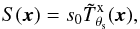 (1)where x indicates the 2D position on the sky (with x = 0 corresponding to the center of the cluster),
  is a normalized cluster spatial profile (normalized so that its central value is 1), and s0 is the cluster central surface brightness. The notation indicates that the cluster profile depends on the apparent size of the cluster through the characteristic cluster scale θs.
Let us imagine that we have an X-ray map of a certain region of the sky in which a cluster is located at position x0, characterized by a profile and a central surface brightness s0. If we denote the convolution of the cluster profile with the point spread function (PSF) of the X-ray instrument Bxray(x) by  , we can express this X-ray map as
 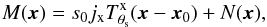 (2)where jx is simply a conversion factor to express the map in any desired units (jx = 1 if the map is expressed in surface brightness units), and N(x) is the noise map, which includes instrumental noise and astrophysical X-ray background. The nature of the X-ray signal means that the map is affected by Poisson noise. Consequently, each pixel of our X-ray map can be characterized as a Poisson random variable with variance equal to the expected value of counts. Let us represent the cluster signal, in counts, by
  , where
  is the expected number of counts at position x and Na(x) is the random noise in addition to this, with zero-mean (⟨Na(x)⟩ = 0) and variance
  . Then, we can rewrite Eq. (2) as
  (3)where Nsig(x) is the additional random noise in the cluster signal that is due to Poisson fluctuations, and Nbk(x) is the background noise. If we define u = s0jx/a as the unit conversion factor from counts to the units of the X-ray map, then we have that Nsig(x) = uNa(x) is a random variable with zero-mean (
 ) and variance equal to
  (4)It is important to keep in mind that, in general, u = u(x) is not constant across the map, but depends on the position. This is because the conversion from counts to surface brightness depends on the exposure time and on the NH column density, which in turn depend on the position. However, for small scales (a few arcminutes), it can be approximated as constant.
If the cluster profile is known, the problem in Eqs. (2) or (3) reduces to estimating the amplitude s0 of a known signal from an observed signal that is contaminated by noise. Generally speaking, if we do not know the probability density function of the noise, we cannot calculate the optimal estimator, that is, the minimum variance unbiased (MVU) estimator. However, we can restrict the estimator to be linear and then find the linear estimator that is unbiased and has minimum variance, that is, the best linear unbiased estimator (BLUE).
We can construct a linear estimator, ŝ0, of the central brightness s0 as a linear combination of the observed data,  (5)where Ψθs can be interpreted as a filter to be applied to the X-ray map. We note that Eq. (5) yields a scalar value if we know the position x0 of the cluster, whereas if it is unknown, we can apply the equation for every possible value of x0 to obtain a ŝ0-map with the same size as the observed map.
If we restrict this linear estimator to be unbiased and to have minimum variance, we obtain the following expression for the filter in Fourier space (the derivation is analogous to that in Haehnelt & Tegmark 1996; Herranz et al. 2002; Melin et al. 2006, 2012):  (6)where
 ![Mathematical equation: \begin{eqnarray} \label{eq:Xray_sigmaMF} \sigma_{\theta_{\rm s}}^2 = \left[j_{\rm x}^2 \sum_{{\vec k}} \frac{\left| T^{\rm{x}}_{\theta_{\rm s}}({\vec k})\right|^2}{{P}({\vec k})} \right] ^{-1} \end{eqnarray}](/articles/aa/full_html/2016/07/aa28366-16/aa28366-16-eq49.png) (7)is, approximately, the background noise variance after filtering (see Appendix A for derivation) and P(k) is the noise power spectrum, given by ⟨N(k)N∗(k′)⟩ = P(k)δ(k − k′). Here and in the remainder of the paper, we use k to denote the two-dimensional spatial frequency, corresponding to x in the Fourier space. All the variables expressed as a function of k are then to be understood as variables in the Fourier space. The filter is determined by the shape of the cluster X-ray signal and by the power spectrum of the noise, hence, the name of X-ray matched filter.
(7)is, approximately, the background noise variance after filtering (see Appendix A for derivation) and P(k) is the noise power spectrum, given by ⟨N(k)N∗(k′)⟩ = P(k)δ(k − k′). Here and in the remainder of the paper, we use k to denote the two-dimensional spatial frequency, corresponding to x in the Fourier space. All the variables expressed as a function of k are then to be understood as variables in the Fourier space. The filter is determined by the shape of the cluster X-ray signal and by the power spectrum of the noise, hence, the name of X-ray matched filter.
Taking the Fourier transform of Eq. (3), we have  (8)When we apply the matched filter given by Eq. (6), the filtered map in Fourier space is
 ![Mathematical equation: \begin{eqnarray} \label{eq:filteredmapFT} \sum_{{\vec k}}^{}\Psi_{\theta_{\rm s}}^\ast({\vec k}) {M}({\vec k})& = & s_{0} j_{\rm x}^2 \sigma_{\theta_{\rm s}}^2 \sum_{{\vec k}}^{} \frac{\left| T^{\rm{x}}_{\theta_{\rm s}}({\vec k}) \right|^2 }{P({\vec k})} \!+ \!j_{\rm x} \sigma_{\theta_{\rm s}}^2 \sum_{{\vec k}}^{} \frac{ T^{\rm{x}\ast}_{\theta_{\rm s}}({\vec k}) }{P({\vec k})} {N_{\rm sig}}({\vec k}) \nonumber\\[3.5mm] \qquad &&\!+\! j_{\rm x} \sigma_{\theta_{\rm s}}^2 \sum_{{\vec k}}^{} \frac{ T^{\rm{x}\ast}_{\theta_{\rm s}}({\vec k}) }{P({\vec k})} N_{\rm bk}({\vec k}), \end{eqnarray}](/articles/aa/full_html/2016/07/aa28366-16/aa28366-16-eq54.png) (9)where the first term on the right-hand side of the equation is equal to s0 (the amplitude of the cluster profile), the third term is the filtered background noise, whose variance is given by Eq. (7) (approximately), and the second term is the filtered Poisson fluctuations on the signal. The variance due to the Poisson fluctuations on the signal, after passing through the filter, can be written as (see derivation in Appendix A)
(9)where the first term on the right-hand side of the equation is equal to s0 (the amplitude of the cluster profile), the third term is the filtered background noise, whose variance is given by Eq. (7) (approximately), and the second term is the filtered Poisson fluctuations on the signal. The variance due to the Poisson fluctuations on the signal, after passing through the filter, can be written as (see derivation in Appendix A)  (10)where n2 is the total number of pixels in the map and the double sum can be computed efficiently by making use of the cross-correlation theorem, as explained in Appendix A. We note that this variance depends on s0, the real value of the central surface brightness. As this is not known in practice, it is necessary to approximate it by its estimated value ŝ0.
Therefore, we can characterize our central brightness estimator ŝ0 as a random variable with mean equal to the true central brightness s0 and variance given by the sum of the variances of the filtered background noise and the filtered Poisson fluctuations on the signal. That is, 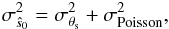 (11)where we have assumed that the Poisson fluctuations on the signal are independent of the background noise, as expected, given their independent origin. Considering this Poisson term in the final variance is essential to correctly characterize the errors on our flux estimation, and it is specially important for bright clusters, where the Poisson noise is dominant over the background noise.
As previously said, if the exact position of the cluster is unknown (or if its accuracy is not high enough), we can apply Eq. (5) for every possible value of x0 and obtain a ŝ0-map with the same size as the observed map. In this case, we also obtain a σPoisson-map that represents the variance due to the Poisson fluctuations on the signal at every position of the map (because u and ŝ0 depend on the position) and a S/N map (ŝ0/σθs) with the same size. The cluster is then detected as a peak in this S/N map, down to a given threshold. In this way, the proposed filter could also be used as a blind detection tool and not only as an estimator of the cluster properties. In this paper we focus on the performance of the filter as an extraction tool (once we know that there is a cluster at a given position); the assessment of its performance as a detector is beyond the scope of this paper and will be undertaken in future work.
It is important to remark that this X-ray matched-filter approach relies on the knowledge of the normalized cluster brightness profile  . In practice this profile is not known, therefore we need to use a theoretical profile that represents the average brightness profile of the clusters we wish to detect as well as possible. Here we assume the average gas density profile from Piffaretti et al. (2011):
 ![Mathematical equation: \begin{eqnarray} \label{eq:densprof} \rho_{\rm gas} \propto \left( \frac{x}{x_{\rm c}}\right)^{-\alpha '} \times \left[1+\left( \frac{x}{x_{\rm c}}\right)^{2}\right] ^{-3\beta'/2+\alpha'/2}, \end{eqnarray}](/articles/aa/full_html/2016/07/aa28366-16/aa28366-16-eq62.png) (12)where xc = 0.303, α′ = 0.525, β′ = 0.768, x = θ/θ500 is the distance to the center of the cluster in θ500 units, and the free parameter θ500 relates to the characteristic cluster scale θs through the concentration parameter c500 (θs = θ500/c500). It can be seen that
(12)where xc = 0.303, α′ = 0.525, β′ = 0.768, x = θ/θ500 is the distance to the center of the cluster in θ500 units, and the free parameter θ500 relates to the characteristic cluster scale θs through the concentration parameter c500 (θs = θ500/c500). It can be seen that  can be written as a GNFW profile given by
 ![Mathematical equation: \begin{eqnarray} \label{eq:pressure_prof} p(x) \propto \frac{1}{\left( c_{500}x\right) ^{\gamma} \left[1+\left( c_{500}x\right) ^{\alpha}\right]^{(\beta-\gamma)/\alpha} } \end{eqnarray}](/articles/aa/full_html/2016/07/aa28366-16/aa28366-16-eq70.png) (13)with α = 2, β = 6β′, γ = 2α′ and c500 = 1 /xc. We therefore describe the squared average density profile using Eq. (13) with the parameters
(13)with α = 2, β = 6β′, γ = 2α′ and c500 = 1 /xc. We therefore describe the squared average density profile using Eq. (13) with the parameters ![Mathematical equation: \begin{eqnarray} \label{eq:xray_param} \left[\alpha, \beta, \gamma, c_{500}\right] = \left[2.0, 4.608, 1.05, 1/0.303\right]. \end{eqnarray}](/articles/aa/full_html/2016/07/aa28366-16/aa28366-16-eq75.png) (14)This expression is convenient to facilitate compatibility with the classical SZ MMF, which uses a GNFW model to describe the cluster profile (see Sect. 3). As previously said, the observed intensity at a given energy in an X-ray map depends on and Λ(Te,z). In the soft X-ray band (below 2 keV), the emissivity Λ(Te,z) is approximately independent of the temperature, so the X-ray emission is approximately proportional to the square of the gas density
(14)This expression is convenient to facilitate compatibility with the classical SZ MMF, which uses a GNFW model to describe the cluster profile (see Sect. 3). As previously said, the observed intensity at a given energy in an X-ray map depends on and Λ(Te,z). In the soft X-ray band (below 2 keV), the emissivity Λ(Te,z) is approximately independent of the temperature, so the X-ray emission is approximately proportional to the square of the gas density  . Thus, the cluster profile
  can be obtained by numerically integrating the cluster 3D squared-density profile (Eq. (13)) along the line of sight.
Finally, to take the effect of beam smoothing affecting the observed signal into account, the cluster profile has to be convolved by the PSF of the instrument, namely Bxray(x). Here we used the X-ray maps of the ROSAT All-Sky Survey, whose PSF is not Gaussian (see Boese 2000; Böhringer et al. 2013). In absence of an analytical expression for the RASS PSF, we have estimated it numerically by stacking observations of X-ray point sources. In particular, we stacked all the point sources in the Bright Source Catalogue (Voges et al. 1999) with Galactic latitude |l| > 30° and computed the azimuthal average of the stack.
On the other hand, the noise power spectrum P(k) can be estimated in practice from the X-ray image itself, after masking and inpainting the cluster region.
2.2. Performance evaluation: simulation results
2.2.1. Description of the simulations
To assess the performance of the proposed X-ray matched filter, we carried out an experiment in which we injected simulated clusters into real X-ray maps and extracted them using the proposed filter, assuming their positions and their sizes are known. The objective of this experiment was to check whether the flux estimated with the matched filter and its associated error bar are consistent with the flux of the injected clusters because a correct photometry at this point will be important for the joint X-ray-SZ algorithm, which relies on the FX/Y500 relation (i.e., the ratio between the X-ray flux of the cluster within R500 in the [0.1–2.4] KeV band and the SZ flux of the cluster within R500). The injection into real maps provides a very realistic environment, with real background contributions and perfectly known cluster characteristics against which to compare the results.
We simulated the clusters as follows. Given the redshift z, the mass M500, and the luminosity L500 of a cluster, we first created a map containing the cluster profile corresponding to the size θ500 of the cluster (calculated from z and M500). This was done by integrating the average profile defined by Eq. (13) with the parameters given in Eq. (14). Then we normalized this map so that its total flux coincided with the flux of the cluster within 5R500 (we assumed that the total flux of the cluster is contained within this radius and calculated it by extrapolating L500 up to 5R500 using the shape of the cluster profile) and convolved this map with the instrument beam. Finally, to obtain a simulated image of the cluster that reproduces the observational noise, we added Poisson fluctuations according to the local photon flux. To this end, we converted the flux at each pixel into counts by using the NH value and the exposure time corresponding to the position where the simulated cluster was going to be injected.
These simulated maps were then added to real X-ray patches centered on random positions of the sky, corresponding to the positions of the simulated clusters. These X-ray patches were constructed in two steps. First, we created an all-sky HEALPix map (Górski et al. 2005) using all the fields of the ROSAT all-sky survey, as described in Appendix B. Second, we projected this HEALPix map onto small 10° × 10° flat patches centered on the cluster position. This way of creating the X-ray patches is, of course, not the only alternative, but we chose it to guarantee compatibility with the SZ MMF that we have used, so that it will be useful for the joint X-ray-SZ algorithm.
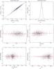 |
Fig. 1 Photometry results of the extraction of simulated MCXC clusters (as described in Sect. 2.2.1) using the proposed X-ray matched filter and assuming the position and size of the clusters are known. Top left panel: extracted versus injected L500. Individual measurements are shown as black dots. The solid blue line shows the line of zero intercept and unity slope and the dashed magenta line the best linear fit to the data. Top right panel: histogram of the difference between the extracted and the injected L500, divided by the estimated |
In particular, we injected 1743 clusters at random positions of the sky, with characteristics (z, M500, and L500) taken from the 1743 clusters in the MCXC catalogue (Piffaretti et al. 2011). Then, we applied the X-ray matched filter described in Sect. 2.1 at each cluster position, fixing the cluster size to the true value. We chose to simulate this sample because it is an X-ray selected sample, and thus it is appropriate for evaluating the performance of our X-ray filter.
2.2.2. Results of the simulations
Figure 1 shows the extraction results for the experiment described above. Figure 1a shows the extracted value of L500 for each cluster as a function of the injected value. We used the redshift in the catalogue to convert from flux to L500. The black dots show the individual measurements, and the red filled circles represent the corresponding averaged values in several luminosity bins. These bin-averaged values were calculated as 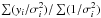 , where yi is the estimated flux of cluster i scaled to L500 units and σi is the estimated
  (also scaled to L500 units) for cluster i. The position of these bin-averaged values in the x-axis was calculated by averaging the injected flux of the clusters in the bin with the same weights that were used to average the extracted flux. The extracted flux follows the injected flux very well, with some dispersion. The best linear fit to these data is given by y = 0.978( ± 0.005)x + 1.2( ± 2.7) × 10-4, which is very close to the unity-slope line, as shown in Fig. 1a.
Figure 1b shows the histogram of the difference between the extracted and the injected value, divided by the estimated standard deviation . Some of the properties of this histogram are summarized in Table 1. In this histogram there is no bias, and the estimated error bars describe the dispersion on the results well (as 68% of the extractions fall in an interval that is close to ± 1σŝ0). The small asymmetry is produced by the fact that we are approximating s0 in Eq. (10) by its estimated value ŝ0, which yields larger error bars for the clusters with overestimated flux and smaller error bars for the clusters with underestimated flux.
Figures 1c to 1f show the difference between the extracted and the injected value, divided by the estimated standard deviation as a function of the redshift, the size, the flux, and the S/N of each cluster. The extraction behaves correctly for all the values of these parameters, and they do not introduce any systematic error or bias in the results.
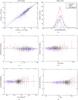 |
Fig. 2 Photometry results of the extraction of the real MCXC clusters using the proposed X-ray matched filter and assuming the position and size of the clusters are known. The six panels are analogous to those in Fig. 1, but comparing the extracted L500 with the published L500. Individual measurements in panels a), c), d), e), and f) are shown as black and blue dots: the black dots correspond to clusters originally detected in RASS, the blue dots to serendipitous clusters. Panel b) shows three histograms that correspond to the RASS clusters (black), the serendipitous clusters (blue), and the complete MCXC sample (red). |
2.3. Performance evaluation: extraction of real clusters
Given that the X-ray matched filter performs well when applied to simulated clusters, the next step is to check its performance on real clusters. This section presents the results of the extraction of known clusters from real X-ray data, assuming that we know their position and size. The objective is to check whether the photometry is still correct for real clusters, and also to quantify the detection probability in this case.
2.3.1. Extraction of MCXC clusters
We started the analysis with the 1743 clusters of the MCXC sample (Piffaretti et al. 2011). We extracted these clusters on 10° × 10° patches centered on the cluster position, following the same procedure as in the previous section. Figures 2 and 3 show the extraction results for this experiment, where we divided the MCXC sample into two subsamples: clusters that were originally detected in RASS and clusters detected in ROSAT serendipitous (deeper) observations.
Figure 2a shows the extracted value of L500 for each cluster as a function of the published value. As in the simulations, we used the redshift in the catalogue to convert from flux to L500. The extracted flux follows the published flux quite well, but the dispersion is larger than in the simulations (Fig. 1a). The best linear fit to these data is given by y = 0.913( ± 0.004)x − 3.76( ± 0.29) × 10-3.
Figure 2b shows the histogram of the difference between the extracted and the published value, divided by the estimated standard deviation . Some of the properties of this histogram are summarized in Table 1. In this histogram we show again that there is no bias for the complete sample, but this time the estimated error bars do not describe the dispersion of the results (as the 68% of the extractions fall in an interval that is almost ± 2σŝ0). It is reasonable to assume that this additional dispersion comes from the difference between the profile used for extraction and the real profile of each particular cluster (see Sect. 2.3.2). We also need to take into account that the published flux has some uncertainties It is difficult to characterize how these affect the dispersion in our histogram because some of the clusters were observed in RASS, that is, using the same data as we used, and others were serendipitous (deeper) observations, for which the published flux is expected to have a lower uncertainty.
Figures 2c to f show the difference between the extracted and the published value, divided by the estimated standard deviation as a function of the redshift, the size, the flux, and the S/N of each cluster. The extraction behaves correctly for almost all the values of these parameters (except for clusters with a very large apparent size, usually very nearby in redshift, which are not the main objects of our interest), and no systematic error is introduced in our region of interest (more distant clusters).
Figure 3 shows the percentage of clusters whose extracted S/N is above a given S/N threshold, which is an indicator of the detection probability of our method. We defined this S/N threshold in terms of the estimated signal ŝ0 divided by the estimated background noise σθs (and not by the estimated total noise ), as done in the classical SZ MMF. For the clusters that were originally detected with RASS observations (the same as we used here), our method finds 95% of them above a S/N threshold of 2, 90% above a S/N threshold of 3, and 84% above a S/N threshold of 4. We recall that the proposed method was designed to be compatible with the MMF used for SZ cluster detection, meaning that it is not specifically optimized for the detection of X-ray clusters. Nevertheless, its performance in this sense is satisfactory. Obviously, our method is not able to detect many of the serendipitous clusters because they were originally detected using deeper observations, but still, some of them are detected: 31%, 20%, and 13% above S/N thresholds of 2, 3, and 4, respectively.
2.3.2. Effect of profile mismatch
As we mentioned above, the additional dispersion we found in the extraction of real clusters may come from the mismatch between the cluster profile and the profile used for the extraction. Since we do not know the real profiles of all the MCXC clusters, we checked the effect of the profile mismatch with the ESZ-XMM sample (Planck Collaboration XI 2011), a well-studied cluster sample composed of 62 clusters detected at high S/N in the first Planck data set and present in XMM-Newton archival data. We chose this sample because its good quality data allows accurately computing the individual cluster profiles.
These 62 clusters were extracted from 10° × 10° patches centered at the cluster positions. We repeated the extraction of these clusters twice. First, we performed the extraction using the average profile defined by Eq. (13) with parameters given in Eq. (14), as previously. Second, we also performed the extraction using the individual profile of each cluster, which was obtained by fitting an AB model (Eq. (12)) to the density profile data used to derive the pressure profiles presented by the Planck Collaboration V (2013), obtained from XMM-Newton observations.
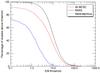 |
Fig. 3 Percentage of MCXC clusters whose extracted S/N, using the proposed X-ray matched filter and assuming the position and size of the clusters are known, is above a given S/N threshold. Red corresponds to the complete MCXC sample, while black and blue correspond to the RASS and serendipitous subsamples, respectively. S/N is defined here as the estimated signal ŝ0 divided by the estimated background noise σθs. |
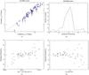 |
Fig. 4 Photometry results of the extraction of the ESZ-XMM clusters using the proposed X-ray matched filter with the average cluster profile and assuming the position and size of the clusters are known. Top left panel: extracted versus published L500. The error bars correspond to the estimated |
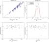 |
Fig. 5 Photometry results of the extraction of the ESZ-XMM clusters using the proposed X-ray matched filter with the individual cluster profiles and assuming the position and size of the clusters are known. The four panels are analogous to those in Fig. 4. The top right panel includes in this case two histograms, one corresponding to the whole ESZ-XMM sample (black) and another corresponding to the ESZ-XMM-A subsample (red), which includes the clusters well within the XMM-Newton field of view. |
Figure 4 shows the results of extracting the 62 ESZ-XMM clusters using the average profile, and Fig. 5 shows the results using the individual profile of each cluster. Figures 4a and 5a show that the extracted flux is consistent with the published flux, as there is no bias (see also Figs. 4b and 5b). The dispersion in Fig. 4b shows the same behaviour as for the MCXC clusters (Fig. 2b): when the average profile is used, the estimated error bars are not enough to describe the dispersion of the results (68% of the extractions fall in the interval ± 2σŝ0). Figure 4c shows that in this case the extracted flux value depends on the shape of the “real” profile of the cluster: if the cluster is very peaked, we tend to overestimate the flux, whereas if the cluster has a flat profile, we tend to underestimate its flux. This effect is especially strong in clusters with larger apparent size θ500, as shown in Fig. 4d. However, when individual profiles, which are better matched to the “real” profiles of the cluster, are used, this dependency disappears, as shown in Figs. 5c and d. The dispersion of the results when we used the individual profiles for the extraction (Fig. 5b) is smaller than when we used the average profile, but it is not completely well characterized by the estimated standard deviation. However, if we focus on subsample ESZ-XMM-A, which includes the clusters with θ500< 12 arcmin (well within the XMM-Newton field of view), the result is much better. We therefore conclude that the additional dispersion when we use the average profile for extraction comes mainly from the profile mismatch.
Since the profile mismatch produces an additional scatter in the estimated flux, it will also produce an additional scatter in the estimated S/N of the clusters. The average S/N, and consequently the global detection probability, will not be affected, but clusters with a peaked profile will be more easily detected than clusters with a flat profile, as in standard detection techniques.
2.4. Practical form of the algorithm
In practice, we do not know the exact profile of the clusters we will detect, so in any case we need to use the average profile. If we assume that the additional dispersion we will have in this case is due to the profile mismatch, we could correct for it using a simple expression depending only on the apparent size of the cluster. Thus, we propose to correct the estimated standard deviation , given in Eq. (11), in the following way: 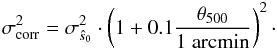 (15)The correction factor was obtained by calculating for the MCXC clusters in several θ500 bins the standard deviation of the difference between the extracted and the published value, divided by the estimated , and checking that it increased roughly linearly with θ500 and tended to 1 when θ500 → 0. It is important to remark that this correction factor is not universal: it depends on the beam, on the cluster sample we are working with (meaning that it depends on the selection function), and on the evolution of the sample. However, this correction is stronger in the regime we are not interested in (clusters with large apparent sizes, hence at low redshift), therefore we consider it as a good approximation for our purposes.
When we apply this empirical correction to the estimated in the MCXC cluster sample, we obtain the histogram in Fig. 6 (see main properties summarized in Table 1), which again shows that there is no bias and that the corrected error bars now describe the dispersion on the results well (as the 68% of the extractions fall in the interval ± 1σ).
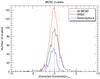 |
Fig. 6 Histogram of the difference between the extracted and the published L500, divided by the standard deviation after correcting for the effect of the profile mismatch (σcorr, scaled to L500 units) for the MCXC clusters extracted with the proposed X-ray matched filter using the average profile and assuming the position and size of the clusters are known. Red corresponds to the complete MCXC sample, while black and blue correspond to the RASS and serendipitous subsamples, respectively. For each color, the central vertical line shows the median value, whereas the other two vertical lines indicate the region inside which 68% of the clusters lie. |
3. Matched multifilter (MMF) for SZ cluster detection
The matched multifilter (MMF) is a well-studied approach that was developed for SZ detection within the Planck mission (Planck Collaboration VIII 2011). It has also been used to detect clusters in other SZ surveys, such as the South Pole Telescope (SPT) survey (Bleem et al. 2015) and the Atacama Cosmology Telescope (ACT) survey (Hasselfield et al. 2013). In this section we recall how it works, since its formulation is used for the joint X-ray-SZ extraction technique.
When CMB photons pass through a galaxy cluster, they can interact with the high-energy electrons in the ICM, gaining energy in the process. This effect, known as thermal Sunyaev-Zel’dovich (SZ) effect, produces a small distortion in the CMB spectrum, which can be observed as a temperature change relative to the mean CMB temperature TCMB (Sunyaev & Zeldovich 1970, 1972). The frequency dependency of this spectral distortion is universal in the non-relativistic limit, while its amplitude, given by the Compton y parameter (proportional to the integral of the gas pressure along the line of sight), depends on the cluster and its spatial profile (Carlstrom et al. 2002; Birkinshaw 1999).
The brightness profile of a cluster as a function of the observation frequency ν can be written as 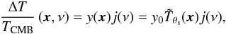 (16)where j(ν) is the universal dependency on frequency of the SZ signal and y(x) is the Compton y parameter at position x, which can be decomposed into y0, the cluster central y-value, multiplied by
  , a normalized cluster spatial profile (normalized so that its central value is 1).
Let us imagine that we have carried out an SZ survey covering a certain region of the sky at Nν observation frequencies νi (i = 1,...,Nν), producing Nν survey maps, and let us denote the instrument beam at observation frequency νi by Bνi(x). Let us further assume there is a cluster in the observed region, at a position x0, characterized by a profile and a central y-value y0. The set of survey maps will contain the SZ signal of the cluster plus noise and can be expressed in matrix form as  (17)where M(x) is a column vector whose ith component is the map at observation frequency νi: M(x) = [M1(x),...,MNν(x)] T, Fθs(x) is a column vector whose ith component is given by Fi(x) = j(νi)Ti(x), where j(νi) is the SZ spectral function at frequency νi and Ti(x) is the normalized cluster profile convolved with the instrument beam at frequency νi (
 ), and N(x) is a column vector whose ith component is the noise map at observation frequency νi: N(x) = [N1(x),...,NNν(x)] T. In this context, noise means anything that is not the SZ signal, that is, instrumental noise and astrophysical foregrounds, such as extragalactic point sources, diffuse Galactic emission, and the primary CMB anisotropy.
There is a clear analogy between the SZ maps defined in Eq. (17) and the X-ray map defined in Eq. (2). Again, if the cluster profile is known, the problem reduces to estimating the amplitude y0 of a known signal from an observed signal contaminated by noise. Therefore, a linear estimator, ŷ0, of y0 can be constructed as a linear combination of the observed data (the Nν observed maps in this case):  (18)where the Nν × 1 column vector Ψθs can be interpreted as a filter whose ith component will filter the map at observation frequency νi. As in the X-ray case, when we restrict this linear estimator to be unbiased and to have minimum variance, we obtain the following expression for the filter in Fourier space (Haehnelt & Tegmark 1996; Herranz et al. 2002; Melin et al. 2006, 2012):
  (19)where
 ![Mathematical equation: \begin{eqnarray} \label{eq:sigma_sz} \sigma_{\theta_{\rm s}}^2 = \left[\sum_{{\vec k}} {\vec F}_{\theta_{\rm s}}^{\rm T}({\vec k}) {\vec P}^{-1}({\vec k}) {\vec F}_{\theta_{\rm s}}({\vec k}) \right] ^{-1} \end{eqnarray}](/articles/aa/full_html/2016/07/aa28366-16/aa28366-16-eq127.png) (20)is the total noise variance after filtering and P(k) is the noise power spectrum, a Nν × Nν matrix whose ij component is given by
(20)is the total noise variance after filtering and P(k) is the noise power spectrum, a Nν × Nν matrix whose ij component is given by  .
.
As in the X-ray case, this approach relies on the knowledge of the cluster brightness profile  , which is not known in practice. Therefore, we again need to use a theoretical profile that represents as well as possible the average brightness profile of the clusters we wish to detect. Melin et al. (2006) used a projected spherical β-profile with β = 2 / 3 to describe as a function of the characteristic scale radius θs. The Planck Collaboration XXIX (2014) assumed that the 3D pressure profile of the cluster followed the GNFW profile of Arnaud et al. (2010), given by Eq. (13) with the parameters
 ![Mathematical equation: \begin{eqnarray} \label{eq:sz_param} \left[\alpha, \beta, \gamma, c_{500}\right] = \left[1.0510, 5.4905, 0.3081, 1.177\right]. \end{eqnarray}](/articles/aa/full_html/2016/07/aa28366-16/aa28366-16-eq135.png) (21)The cluster profile can be then obtained by numerically integrating the cluster 3D pressure profile in Eq. (13) along the line of sight. We will also adopt this model for the SZ cluster profile.
(21)The cluster profile can be then obtained by numerically integrating the cluster 3D pressure profile in Eq. (13) along the line of sight. We will also adopt this model for the SZ cluster profile.
Finally, as in the X-ray case, we need to convolve this cluster profile by the instrument beams Bνi(x). We used the six highest frequency Planck maps, from 100 to 857 GHz, and assumed that the PSF of the instrument is Gaussian, with FWHM between 9.66 and 4.22 arcmin, depending on the frequency, as shown in Table 6 of Planck Collaboration VIII (2016).
4. Joint extraction of galaxy clusters on X-ray and SZ maps
In this section, the proposed joint X-ray-SZ extraction algorithm is described and evaluated.
4.1. Description of the algorithm
The main idea of our joint extraction algorithm is to consider the X-ray map as an additional SZ map at a given frequency and to introduce it, together with the other SZ maps, into the classical SZ-MMF described in Sect. 3. To do so, we need to convert our X-ray map into an equivalent SZ map at a reference frequency νref, leveraging the expected FX/Y500 relation. The details of this conversion are described in Appendix B.
Once the X-ray map is expressed in the same units as the SZ maps (we used ΔT/TCMB units), the MMF described in Sect. 3 can be applied almost directly to the complete set of maps (the original Nν SZ maps obtained at observation frequencies ν1,...,νNν and an additional SZ map at the reference frequency νref, obtained from the X-ray map). If there is a cluster in the observed region at position x0, characterized by an SZ profile  , a central y-value y0, and an X-ray profile , taking the conversion from the original X-ray map to its equivalent SZ map into account, this set of maps can be expressed in matrix form using Eq. (17) again, where M(x), Fθs(x) and N(x) are now column vectors with Nν + 1 components, defined as
![Mathematical equation: \begin{eqnarray} && {\vec M}({\vec x})=[M_{1}({\vec x}), ..., M_{N_\nu}({\vec x}), M_{\rm ref}({\vec x})]^{\rm T},\\ \label{eq:F_joint} &&{\vec F}_{\theta_{\rm s}}({\vec x}) = [j(\nu_{1}) T_{1}({\vec x}), ..., j(\nu_{N_{\nu}}) T_{N_{\nu}}({\vec x}), C j(\nu_{\rm ref}) {T}^{\rm{x}}_{\theta_{\rm s}}({\vec x})]^{\rm T},\\ && {\vec N}({\vec x}) = [N_{1}({\vec x}), ..., N_{N_\nu}({\vec x}), N_{\rm ref}({\vec x})]^{\rm T}, \end{eqnarray}](/articles/aa/full_html/2016/07/aa28366-16/aa28366-16-eq142.png) where ,
where ,  and the constant C is the ratio of the integrated fluxes of the normalized SZ and X-ray 3D profiles up to R500, that is,
  (25)The subindex “ref” denotes the component corresponding to the additional map. Therefore, Nref(x) contains two types of noise: the background noise and the random noise in addition to the cluster signal that is due to Poisson fluctuations, as described in Sect. 2 (Nref(x) = Nsig(x) + Nbk(x)).
Again, if the cluster profile is known, the problem reduces to estimating the amplitude y0 of a known signal from an observed signal contaminated by noise and, as before, its best linear unbiased estimator ŷ0 is given by Eqs. (18)–(20), where the new (Nν + 1) × 1 column vector Ψθs can be interpreted as a filter whose ith component will filter the map at observation frequency νi,  is, approximately, the background noise variance after filtering, Fθs is defined in Eq. (23) and P(k) is the noise power spectrum, a (Nν + 1) × (Nν + 1) matrix whose ij component is given by . Considering that the noise in the X-ray map and the SZ maps is uncorrelated, we can write the noise power spectrum as
 ![Mathematical equation: \begin{eqnarray} \label{eq:P_joint} {\vec P}({\vec k}) = \left[\begin{array}{c c} {\vec P}_{\rm SZ}({\vec k}) & {\vec 0}_{N_\nu \times 1} \\ {\vec 0}_{1 \times N_\nu} & P_{\rm X}({\vec k})\\ \end{array}\right], \end{eqnarray}](/articles/aa/full_html/2016/07/aa28366-16/aa28366-16-eq152.png) (26)where PSZ(k) is the noise power spectrum of the SZ maps, defined in Sect. 3, PX(k) is the noise power spectrum of the X-ray map, defined in Sect. 2, and 0n × m denotes a vector with n rows and m columns whose elements are all equal to 0.
(26)where PSZ(k) is the noise power spectrum of the SZ maps, defined in Sect. 3, PX(k) is the noise power spectrum of the X-ray map, defined in Sect. 2, and 0n × m denotes a vector with n rows and m columns whose elements are all equal to 0.
As in the X-ray case, the filtered map is composed of three terms: the amplitude of the cluster profile y0, plus the filtered background noise and the filtered Poisson fluctuations on the X-ray signal. The variance of the filtered background noise is given (approximately) by Eq. (20) and the variance due to the Poisson fluctuations on the signal, after passing through the filter, can be written as  (27)where n2 is the total number of pixels in the map, u is the unit conversion factor from counts to the units of the SZ-equivalent X-ray map (ΔT/TCMB units in this case), and the double sum can be computed efficiently by making use of the cross-correlation theorem, as explained in Appendix A. The derivation of this expression is completely analogous to that of the X-ray case included in Appendix A, assuming uncorrelated X-ray and SZ noise. We note that this variance depends on y0, the real value of the central y-value. As this is not known in practice, it is necessary to approximate it by its estimated value ŷ0.
Therefore, we can characterize our central y-value estimator ŷ0 as a random variable with mean equal to the true central y-value y0 and variance given by the sum of the variances of the filtered background noise and the filtered Poisson fluctuations on the signal. That is,  (28)where we have assumed that the Poisson fluctuations on the signal are independent of the background noise.
As in the previous cases, the cluster profile is not known, so we will need to approximate it by the theoretical profile that best represents the clusters we wish to detect. In this case, we again assumed the GNFW profile given by Eq. (13), with parameters given by Eqs. (21) and (14) for the components corresponding to the original SZ maps and the additional X-ray map, respectively. The cluster profile is then obtained by numerically integrating these GNFW profiles along the line of sight. Finally, as in the previous cases, we need to convolve this cluster profile by the instrument beams, for which we used the beams defined in Sects. 2 and 3.
K-correction for Tref = 7 keV.
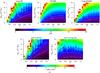 |
Fig. 7 Top panels: S/N of the clusters extracted with the proposed X-ray matched filter (left panel), the classical SZ MMF (middle panel), and the proposed X-ray-SZ MMF (right panel), averaged in different mass and redshift bins. White lines indicate smoothed isocontours corresponding to a S/N of 3, 4, and 5. White bins indicate a S/N greater than 20. Bottom panels: average difference between the S/N obtained with the proposed X-ray-SZ MMF and the S/N obtained with SZ MMF (left panel) and the X-ray MF (right panel). White lines indicate smoothed isocontours corresponding to a difference in S/N of 1, 2, and 3. White bins indicate a difference in S/N greater than 10. |
4.2. Performance evaluation: gain with respect to single-survey extractions
The goal of our joint matched filter is to improve the cluster detection rate with respect to the classical SZ MMF approach. Our technique gives a priori a higher S/N than the SZ MMF alone due to the inclusion of the additional map, so it may improve the detectability of galaxy clusters. Clearly, the false-detection rate should also be kept at a low value for a good detector performance. This latter point is beyond the scope of the present work, but we will explore it in a future work. It can be proven that the filtered background noise in the proposed algorithm is related to the filtered background noise of the SZ and the X-ray maps by the following relation:  (29)where σJOINT is given by Eq. (20) (with Fθs and P defined in Eqs. (23) and (26)), and σSZ and σXray are calculated in an analogous way, but just using the Nν SZ components of Fθs and PSZ in the first case, and the X-ray component of Fθs and PX in the second case. According to the previous relation, if the signal is perfectly estimated, there is always a gain in S/N with respect to using a single-map extraction (
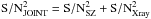 ). In practice, however, we may not always see this gain in S/N because of estimation errors.
In this section we compare the performance of the proposed joint matched filter to that of the classical SZ MMF and the proposed X-ray matched filter in terms of gain in the S/N of the extracted objects, or equivalently, in terms of detection probability (note that when we define a cluster to be detected when its S/N is above a given threshold, the S/N gain will translate into a higher detection rate). This comparison is made both with simulated and real clusters.
4.2.1. Description of the simulations
For this comparison, we first carried out a series of experiments in which we injected simulated clusters into real SZ and X-ray maps and extracted them using the three considered methods: the classical SZ MMF described in Sect. 3, the proposed X-ray matched filter, and the proposed joint matched filter. In the three cases, we assumed that the positions and sizes of the clusters are known, and in the joint MMF case, we further assumed that their redshifts are known. For the injections, we used the six highest frequency Planck all-sky maps and the X-ray all-sky HEALPix map that we constructed from RASS data (see Appendix B).
Given the redshift z, the mass M500, the luminosity L500 and the SZ flux Y500 of each cluster, the clusters to inject into the X-ray maps were simulated as explained in Sect. 2.2. The simulation of the corresponding SZ clusters was done similarly: we first created a map containing the SZ cluster profile corresponding to the size θ500 of the cluster (calculated from z and M500). This was done by integrating the average profile defined by Eq. (13) with the parameters given in Eq. (21). Then we normalized this map so that its total SZ flux coincided with the SZ flux of the cluster within 5R500. This total SZ flux was calculated by extrapolating Y500 up to 5R500 using the shape of the cluster profile. Finally, we convolved this map with the six different Planck beams and applied the SZ spectral function for the corresponding Planck frequencies to obtain a set of Nν = 6 images of the simulated cluster. These simulated maps were then added to real 10° × 10° patches centered on the (random) positions of the simulated clusters.
We divided the redshift-mass plane into 32 bins (four mass bins: 2–4, 4–6, 6–8, and 8–10 × 1014 M⊙ and eight redshift bins: 0.1–0.3, 0.3–0.5, 0.5–0.6, 0.6–0.7, 0.7–0.8, 0.8–0.9, 0.9–1.0, and 1.0–1.1), and for each bin, we injected 1000 clusters at random positions of the sky, with z and M500 uniformly distributed in the bin. L500 was calculated from the L-M relation in Arnaud et al. (2010), Planck Collaboration XI (2011), including the scatter σlog L = 0.183, and Y500 was calculated from the nominal value of L500 (from L-M relation without scatter), assuming a given L500 − Y500 relation. For these simulations we assumed the relation found by the Planck Collaboration I (2012): ![Mathematical equation: \begin{eqnarray} \label{eq:FxY500relation} \frac{F_X \left[{\rm erg s^{-1} cm^{-2}}\right]}{Y_{500} \left[{\rm arcmin}^{2}\right]} = 4.95 \times 10^{-9} \cdot E(z)^{5/3} (1+z)^{-4} K(z). \end{eqnarray}](/articles/aa/full_html/2016/07/aa28366-16/aa28366-16-eq178.png) (30)The K-correction was obtained by interpolating in Table 2, which was calculated using a mekal model for a reference temperature of Tref = 7 keV (corresponding approximately to the median of the clusters above z = 0.3). Since we did not include scatter in the Y-M relation (because it is much smaller than the L-M scatter), the σlog L = 0.183 scatter translates directly into a FX/Y500 scatter. Then we applied the three extraction methods at each cluster position. For the X-ray-SZ matched filter, we assumed the same FX/Y500 relation used in the injection (Eq. (30)), with the real redshift of the clusters, to convert the X-ray map into an equivalent SZ map.
(30)The K-correction was obtained by interpolating in Table 2, which was calculated using a mekal model for a reference temperature of Tref = 7 keV (corresponding approximately to the median of the clusters above z = 0.3). Since we did not include scatter in the Y-M relation (because it is much smaller than the L-M scatter), the σlog L = 0.183 scatter translates directly into a FX/Y500 scatter. Then we applied the three extraction methods at each cluster position. For the X-ray-SZ matched filter, we assumed the same FX/Y500 relation used in the injection (Eq. (30)), with the real redshift of the clusters, to convert the X-ray map into an equivalent SZ map.
4.2.2. Results of the simulations
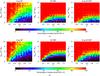 |
Fig. 8 Estimated completeness of the proposed X-ray matched filter (left panels), the classical SZ MMF (middle panels) and the proposed X-ray-SZ MMF (right panels) for a S/N threshold of 3.0 (top panels) and 4.5 (bottom panels), in different redshift-mass bins. |
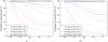 |
Fig. 9 Estimated completeness of the proposed X-ray matched filter (dashed lines), the classical SZ MMF (dotted lines), and the proposed X-ray-SZ MMF (solid lines) as a function of redshift for a S/N threshold of 3.0 (left panel) and 4.5 (right panel). The different colors correspond to different mass bins, as indicated in the legend. |
Figure 7 shows the average S/N of the injected clusters using the three different methods and the gain in S/N of the joint MMF with respect to the single-survey methods. For this computation, we excluded the clusters injected in the Galactic region, where the foreground emission is very high, using the cosmology mask defined by the Planck Collaboration XXVII (2016). We first note in this figure the different performance that we achieve using the X-ray information from RASS and the SZ information from Planck. While the dependence on redshift and mass is quite steep for the X-ray case, for the SZ case it becomes flatter at high redshift (because the SZ signal is insensitive to the (1 + z)4 dimming), which makes high-redshift clusters easier to detect using the SZ information. For this particular configuration, for example, the S/N = 5 and S/N = 3 isocontours of these two cases cross at z = 0.5 and z = 0.6, respectively, meaning that below this redshift the X-ray information provided by the RASS survey is more significant than the one provided by the Planck survey, while for higher redshift SZ maps become more helpful. This figure also shows that adding the X-ray information to the SZ maps improves the S/N over the whole range of redshifts and masses, although the gain with respect to using only the SZ information decreases with increasing redshift and with decreasing mass, as expected, since the amount of information brought by the X-ray map diminishes in these cases. For example, the typical S/N for a cluster with M500 = 5 × 10¹⁴ M⊙ and z = 0.5 is around 5.4 for the X-ray MF, around 5.2 for the SZ MMF, and around 7.5 for the X-ray-SZ MMF, while the same cluster at z = 1.0 will typically have a S/N around 2.8 for the X-ray MF, around 4.4 for the SZ MMF, and around 5.2 for the X-ray-SZ MMF.
Figures 8 and 9 show the percentage of clusters found above S/N = 4.5 and S/N = 3.0 in different mass and redshift bins, that is, the estimated completeness, for the three different methods. These figures show that adding the X-ray information improves the detection rate over the whole range of redshifts and masses, although the gain with respect to using only the SZ information decreases with redshift, as expected. From the 20%, 50%, and 80% completeness levels overplotted in Fig. 8, the advantage of using the joint algorithm is clearly visible because the detection limit is pushed towards higher redshift and lower mass clusters. We checked that the SZ results are compatible with the theoretical expectations using the ERF error function approximation (Planck Collaboration XXIX 2014) and with the results presented by the Planck Collaboration XXVII (2016). We reach a 100% detection rate for the highest mass bin with the SZ and the joint MMF. Interestingly, a low, but non-zero, fraction of the low-mass and high-redshift clusters can also be detected. We checked that these are real clusters and not only noise peaks or other objects in the maps because the extraction at the same positions but without the injected clusters provides only one false detection in the last bin (0.1%) with the SZ MMF and no false detection with the other two methods.
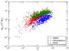 |
Fig. 10 MCXC and PSZ2 cluster samples in the mass-redshift plane. The MCXC sample is divided into RASS and serendipitous subsamples. |
4.2.3. Extraction of real clusters
The analysis presented above illustrates the advantage of using the proposed X-ray-SZ MMF on simulated clusters. However, the simulations are based on some assumptions that may not hold in the real world, for example, an ideal cluster profile or a perfectly known FX/Y500 relation. To check whether the expected behavior is maintained in a more realistic scenario, we carried out another set of experiments in which we extracted known real clusters, using the three methods. In particular, we extracted the 1743 clusters of the MCXC sample (Piffaretti et al. 2011), for which we already presented the X-ray extraction results in Sect. 2.3, and the 926 confirmed clusters with redshift estimates of the second Planck SZ (PSZ2) catalogue (Planck Collaboration XXVII 2016) that were detected with the MMF3 method, which we used as basis of our algorithm (described in Sect. 3). Figure 10 shows these clusters in the mass-redshift plane. These two samples were chosen to analyse the possible differences in the performance of the proposed joint X-ray-SZ on X-ray selected clusters, as the MCXC clusters, and on SZ selected clusters, as the PSZ2 clusters.
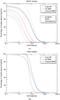 |
Fig. 11 Percentage of MCXC (top panel) and PSZ2 (bottom panel) clusters extracted with the proposed X-ray matched filter (green), the classical SZ MMF (red), and the proposed X-ray-SZ MMF (blue) whose S/N is above a certain S/N threshold. In the top panel, the complete MCXC sample (solid lines) is divided into RASS (dotted lines) and serendipitous clusters (dashed lines). |
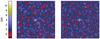 |
Fig. 12 S/N maps obtained in the extraction of cluster PSZ2 G156.26+59.64 using the SZ-MMF (left) and the X-ray-SZ MMF (right). The S/N at the cluster position improves from 5.38 to 11.92. The angular size of the images is 3°. The cluster redshift is z = 0.59. We have masked an X-ray source to the bottom-left of the cluster. |
The MCXC clusters were extracted on 10° × 10° patches centered on the cluster position, fixing the cluster size to the true value. In this case, we assumed the following FX/Y500 relation to convert the X-ray map into an equivalent SZ map: ![Mathematical equation: \begin{eqnarray} \label{eq:FxY500relation_PXCC} \frac{F_X \left[{\rm erg s^{-1} cm^{-2}}\right] }{Y_{500} \left[{\rm arcmin}^{2}\right] } = 7.41 \times 10^{-9} \cdot E(z)^{5/3} (1+z)^{-4} K(z). \end{eqnarray}](/articles/aa/full_html/2016/07/aa28366-16/aa28366-16-eq191.png) (31)This expression was obtained from the
(31)This expression was obtained from the  relation found by the Planck Collaboration X (2011) for this cluster sample, with the approximation
  for a pivot luminosity of 1 erg/s. We note the difference in the normalization with respect to Eq. (30). In Sect. 4.4 we investigate the effects of the assumed FX/Y500 relation in detail.
For the PSZ2 sample, we used the same extraction procedure as for the MCXC clusters, but in this case we assumed the general FX/Y500 relation defined in Eq. (30), since there is no better relation available for this particular sample. We also allowed for a small freedom (2.5 arcmin) in the position to account for the lower position accuracy provided by the PSZ2 catalogue.
Due to the small number of clusters in these samples, we cannot statistically analyse the results in different mass and redshift bins, as we did for the simulations, but we can show the global behaviour. Figure 11a shows how the proposed joint algorithm increases the detection probability with respect to the X-ray matched filter and the classical SZ MMF for the MCXC clusters. In comparison with the extraction of the MCXC clusters using the X-ray matched filter (see Sect. 2.3), the joint algorithm is able to detect slightly more clusters: 97%, 93%, and 87% of the RASS clusters (and 36%, 23%, and 14% of the serendipitous clusters) for S/N thresholds of 2, 3, and 4, respectively. As expected, for this X-ray selected sample, including the SZ information slightly improves the detection probability, while adding the X-ray map to the classical SZ MMF has a strong effect. Figure 11b shows the percentage PSZ2 clusters detected above a given S/N threshold for the three detection methods. For this SZ selected sample, the proposed joint algorithm again increases the detection probability with respect to the X-ray matched filter and the classical SZ MMF alone. In Appendix C we present a more detailed comparison of the estimated S/N obtained for the MCXC clusters and the PSZ2 clusters using the three detection methods as a function of redshift and mass, which shows that there is a S/N gain for most of the clusters, even for high redshift. We therefore conclude that in comparison with the single-survey filters, the proposed X-ray-SZ MMF provides a better significance of the extracted clusters, helping to detect clusters up to higher redshift and lower mass. Of course, to use the proposed technique as a blind detection tool, the detection probability not only has to be high, but the false-detection rate must also be kept at a low value. The latter point is beyond the scope of this paper, but will be investigated in future work.
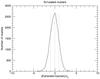 |
Fig. 13 Histogram of the difference between the extracted and the injected L500, divided by the estimated |
As a visual illustration of the gain we can achieve, Fig. 12 shows the S/N maps obtained in the extraction of cluster PSZ2 G156.26+59.64, a massive cluster at z = 0.59, using the SZ MMF and the X-ray-SZ MMF. In these images the improvement in S/N is obvious.
4.3. Performance evaluation: photometry
Since the joint matched filter provides an estimate of the flux of the detected clusters by combining the X-ray and SZ information and assuming a given underlying relation, it is important to check whether the provided photometry is accurate and how it depends on the assumptions. In this section we assess the performance of the proposed joint matched filter in terms of photometry, through simulations and through extraction of real clusters.
First, with the aim of checking that the photometry results are correct in the ideal setting, we carried out an injection experiment, similar to the one presented in the previous section, but without scatter in the L-M relation. We checked that the extracted flux follows the injected flux very well, with a linear fit that is very close to the unity-slope line (y = 1.0067( ± 0.0015)x − 9.8( ± 0.9) × 10-2). Figure 13 shows the histogram of the difference between the extracted and the injected flux, divided by the estimated standard deviation  corresponding to this experiment. This histogram shows that there is no bias and that the estimated error bars describe the dispersion on the results well (as 68% of the extractions fall in an interval that is close to ±1). We also checked that the extraction behaves correctly for all the values of redshift, size, flux, and S/N and that these parameters do not introduce any systematic error or bias in the results.
From this experiment, we conclude that the combined X-ray-SZ matched filter performs well when applied to ideal simulated clusters. However, the simulations are based on some assumptions that may not hold in the real world (ideal cluster profiles, known L500/Y500 relation with no scatter). Therefore, the final step in this paper is to check the performance of the proposed filter on real clusters. In the following, we present the photometry results from the extraction of known clusters on real SZ and X-ray data, assuming that we know their position, size, and redshift. In particular, we focused on the MCXC and the PSZ2 samples presented in Sect. 4.2.
Figure 14 shows the extraction results for the MCXC sample. Figure 14a shows the extracted value of L500 for each cluster as a function of the published value. As in the simulations, we used the redshift in the catalogue to convert from flux to L500. The extracted flux follows the published flux quite well, but the dispersion is larger than in the simulations. The best linear fit to these data is given by y = 0.972( ± 0.004)x + 3.03( ± 0.28) × 10-3, which is very close to the unity-slope line, as shown in Fig. 14a. The subplot shows the histogram of the difference between the extracted and the published flux, divided by the estimated standard deviation . Some of the properties of this histogram are summarized in Table 3. This histogram again shows that there is no bias, but that this time the estimated error bars are not large enough to describe the dispersion of the results (as the 68% of the extractions fall in an interval that is almost ± 2σŷ0). This additional dispersion may come from the difference between the profile used for extraction and the real profile of each particular cluster, as in the X-ray case, but also from the scatter in the real L500/Y500 relation (we refer to Appendix D for an illustration based on simulations of how this scatter increases the dispersion in the extracted flux).
Since in practice the exact profile of the clusters we will detect and their L500/Y500 are unknown, we will multiply the estimated value of , given in Eq. (28), by a correction factor to embed the additional dispersion into the estimated standard deviation, as we did in the X-ray case. In particular, we will use the following expression, which was obtained similarly to the correction factor for the X-ray case, 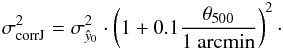 (32)As for the X-ray case, this correction factor is not universal. However, the correction is stronger in the regime we are not interested in (clusters with large apparent sizes), therefore we consider it as a good approximation for our purposes.
By applying this empirical correction, we obtain the histogram in Fig. 14b (see main properties on Table 3), which again shows that there is no bias and that the corrected error bars now describe the dispersion on the results well (as the 68% of the extractions fall in the interval ± 1σ). Figures 14c to f show the difference between the extracted and the published flux, divided by the corrected as a function of the redshift, the size, the flux, and the S/N of each cluster. The extraction behaves correctly for almost all the values of these parameters (except for clusters with very large apparent size or that are very close, which are not the objects of our interest), and that no systematic error is introduced in our region of interest (more distant clusters).
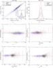 |
Fig. 14 Photometry results of the extraction of the MCXC clusters using the proposed X-ray-SZ filter with the average cluster profile and assuming the position, size, and redshift of the clusters are known. The top left panel is analogous to the top left panel of Fig. 2, and its subpanel shows the histogram of the difference between the extracted and the published L500, divided by the estimated |
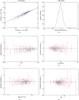 |
Fig. 15 Photometry results of the extraction of the PSZ2 clusters using the proposed X-ray-SZ filter with the average cluster profile and assuming the position, size, and redshift of the clusters are known. The six panels are analogous to those in Fig. 14, with panel e showing the difference between the extracted and the published L500, divided by the corrected standard deviation σcorrJ as a function of the mass of each cluster instead of as a function of the flux as in Fig. 14e. |
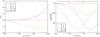 |
Fig. 16 Expected values of the extracted flux (left panel) and the estimated S/N (right panel) when an incorrect FX/Y500 relation is assumed. The figure shows the ratio with respect to the expected value corresponding to the true relation as a function of the relative contribution of the X-ray and SZ background noises ω (low ω values represent better SZ maps and high ω values correspond to a better X-ray map). Different values of a = (FX/Y500)assumed/ (FX/Y500)true are shown in different colors, according to the legend. |
Figure 15 shows the extraction results for the PSZ2 sample. Figure 15a shows the extracted value of L500 for each cluster as a function of the published value. As before, we used the redshift in the catalogue to convert from flux to L500. Figure 15b shows the histogram of the difference between the extracted and the published flux, divided by σcorrJ, the estimated standard deviation corrected according to Eq. (32). Some of the properties of this histogram are summarized in Table 3. This histogram shows a small negative bias and a dispersion that is higher than expected. The bias arises because the assumed FX/Y500 relation is not perfectly suited for this sample of clusters. The additional dispersion may again stem from the scatter in the relation and from the profile mismatch, and the correction that we found for the MCXC clusters is not perfect in this case. Figures 15c to 15f show the difference between the extracted and the published flux, divided by the corrected as a function of the redshift, the size, the mass, and the S/N of each cluster. In the range we are interested in, these parameters do not introduce additional biases.
4.4. Considerations on the FX/Y500 relation
A key point of the joint algorithm is the expected FX/Y500 relation that is used to convert the X-ray map into an additional single-frequency SZ map. If the assumed relation does not correspond to the true relation for a given cluster, the estimated flux for that cluster will be incorrect, and so will its estimated S/N. We have already pointed out the effects on photometry in the previous section, where we showed with the extraction of the MCXC clusters that although we know the average FX/Y500 relation for this cluster sample, the intrinsic dispersion in this relation produces an additional scatter in the estimated flux. We also showed with the extraction of the PSZ2 clusters that if we do not precisely know the average FX/Y500 relation for the clusters we extract, we will get a bias in the extracted flux. In this section, we quantitatively analyse the effects of using an incorrect FX/Y500 relation on the photometry and also on the estimated S/N.
Let us consider a given cluster for which the assumed relation differs from the true relation by a factor a defined as follows: 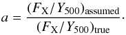 (33)It can be proven that the expected values for the extracted joint flux and the S/N of that cluster are given by
  where
where  (36)and y0 and S/N = y0/σθs are the expected values when the true FX/Y500 relation is known.
Figure 16 shows the effect of using an incorrect FX/Y500 on the extracted flux and the estimated S/N. The joint flux can be severely affected, especially when the noise of the X-ray map is small in comparison to the noise of the SZ maps. For example, when we use a relation that is a factor of two higher than the true one, the estimated flux can be divided by two. The figure also shows that when the assumed relation is smaller than the true relation (a< 1), the joint flux is overestimated (so the SZ flux obtained from it will be also overestimated, and the corresponding estimated X-ray flux will be underestimated), while when the assumed relation is higher (a> 1), the joint flux is underestimated. For the S/N the effect of using an incorrect FX/Y500 is not as significant as for the flux. The S/N is always underestimated with respect to the S/N that we would obtain with the correct FX/Y500 relation. However, the ratio between the two is bounded: there is a minimum at ω = 1 /a, whose value is  (note that this value is the same for a and 1 /a). For example, if we are incorrect by a factor of two in the FX/Y500 relation, we will obtain down to 94% of the S/N, while if we are incorrect by a factor of three, we will obtain down to 87% of the S/N. Given that we do not expect to deviate from the true relation by much more than this, we can conclude that the estimated S/N will be affected by at most a few percent, which means that the effect on the detection probability will be weak as well.
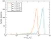 |
Fig. 17 Histogram of the relative contribution of the X-ray and SZ background noises ω for the RASS and Planck maps. |
To estimate the effect of using an incorrect FX/Y500 relation with this figure, we still have two questions to answer. First, what is the range of ω values that we have in our maps? And second, what is the range of values that we expect for a? Figure 17 answers the first question, showing the regime of ω values that we have in our maps, that is, the six highest frequency Planck all-sky maps and the X-ray all-sky map that we constructed from RASS data. The histograms were calculated by filtering 1000 random patches of the sky with different filter sizes. The value of ω slightly depends on the size of the filter, while it depends much more on the reference redshift that we use to convert the X-ray map into an equivalent SZ map, since  is proportional to (FX/Y500)2(z).
To illustrate the effect of the FX/Y500 relation that is assumed in the extraction, we carried out an experiment in which we simulated clusters according to the Tinker mass function (Tinker et al. 2008), with M500> 3 × 10¹⁴ M⊙ and 0 <z< 1. In this simulation, we injected clusters following, on average, the FX/Y500 relation in Eq. (30), and we added a scatter of σlog L = 0.183, which is the typical scatter found in the L − M relation (Arnaud et al. 2010; Planck Collaboration XI 2011). A total of 1787 clusters were injected in the maps and extracted using the proposed joint matched filter, assuming three different FX/Y500 relations for the extraction (similar to Eq. (30), but with different normalizations: 3.30, 4.95 and 7.40). Although assuming a FX/Y500 relation different from the real one introduces, as discussed previously, errors in the estimated flux, it has no strong effect on the S/N of the detected clusters and therefore does not affect the detection probability of the method, as illustrated in Fig. 18. We also checked that the assumed FX/Y500 does not have an effect on the estimated S/N of the joint extraction of the real MCXC clusters, which makes the detection robust against possible errors in the assumed relation.
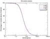 |
Fig. 18 Percentage of simulated clusters (as described in Sect. 4.4) whose extracted S/N, using the proposed X-ray matched filter and assuming the position, size, and redshift of the clusters are known, is above a given S/N threshold. The different colors correspond to different normalizations of the FX/Y500 relation assumed for the extraction, as indicated in the legend. |
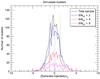 |
Fig. 19 Histogram of the difference between the extracted and the injected L500, divided by the estimated |
Regarding the second question, the FX/Y500 relation for a given cluster is not a fixed quantity: it depends on the redshift and on the luminosity of the cluster, and even for a given redshift and luminosity, it also has some intrinsic dispersion. In the following, we summarize how these variables are expected to affect the joint extraction results:
-
Redshift: when we search for clusters whose redshift we do not know, we assume a reference redshift zref for all the potential clusters in our maps. For example, if we take an intermediate redshift of 0.5 as reference, and assuming the FX/Y500 only depends on the redshift as in Eq. (30), then the values of a would range between 0.5 and 1.7 for clusters at z = 0.1 and z = 1, respectively. Since the FX/Y500 relation decreases with redshift, if the real redshift of a cluster is higher (or lower) than zref, then a> 1 (a< 1), so that its SZ flux will be underestimated (or overestimated). Regarding the S/N, the effect of using a reference redshift that is different from the cluster redshift is limited. For example, if we take an intermediate redshift of 0.5 as reference, then the S/N for a cluster at z = 1 will only be 96.6% (at most) of the one we would obtain with the correct redshift.
-
Luminosity: the FX/Y500 relation is calculated by approximating the Y500 − L500 relation by a unity-slope relation for a pivot luminosity. If this reference luminosity is higher than the true luminosity, the assumed relation will be smaller (a< 1). For example, the FX/Y500 relation in Eq. (30) comes from the Y500 − L500 relation derived by the Planck Collaboration XI (2011), for a pivot luminosity of 7 × 1044 erg/s. For clusters with luminosities ranging from 1042 to 1046 erg/s, the difference between Eq. (30) and the FX/Y500 value derived from the original Y500 − L500 relation (without approximations) ranges between a = 0.88 and a = 1.05. This clearly is a second-order effect, and it could be further reduced by using an iterative process (assume luminosity, then extract flux for the corresponding relation, calculate new relation corresponding to estimated luminosity, re-extract, and so on), which means that we do not need to worry about it.
-
Intrinsic scatter: even if we knew the redshift and luminosity of our cluster, there is an intrinsic dispersion in the FX/Y500 relation. This will introduce an additional scatter in the estimated flux (see Appendix E for an illustration), as we have mentioned before, and slightly reduce the S/N of the clusters.
Finally, we should note that the average FX/Y500 depends on the sample, therefore selection effects play a role in its average value. If we take an average FX/Y500 relation that does not correspond to the true average FX/Y500 relation of the clusters we detect, the flux of the sample will be biased. To illustrate the effect of the last point, we analysed the photometry results from the last simulation (clusters following the Tinker mass function). Figure 19 shows how the histogram of the difference between the extracted and the injected value, divided by the estimated standard deviation , changes depending on the selection of the sample. For the complete sample, we can see that there is no bias, but because of the scatter in the L500 − Y500 relation, the estimated error bars are not enough to fully describe the dispersion on the results. If we select only those clusters for which the S/N in the Planck maps is above a given threshold, an increasing positive bias appears.
From these considerations we can conclude that the proposed X-ray-SZ matched filter will provide a higher detection probability than single-survey filters, even if we have some error in the assumed FX/Y500 relation, since the S/N of the detected clusters is only slightly affected by these errors. However, not knowing the value of the FX/Y500 relation has a stronger effect on the photometry, which means that the fluxes estimated by the joint algorithm will not be precise. It is therefore better to keep the independent flux estimates from the two single-survey filters instead of using the combined flux that depends on our knowledge of the FX/Y500 relation.
We remark that the effects described in this section are averaged effects, that is, they refer to the expected values of the flux and S/N. In addition, there will be a scatter caused by the filtered noise, which will be smaller for clusters with higher flux.
5. Conclusions
In this paper we have proposed a matched-filter approach to extract the signal from galaxy clusters using X-ray and SZ maps simultaneously. The method is based on the combination of the classical SZ MMF and an analogous single-frequency matched filter developed for X-ray maps. The combination relies on the physical relation between X-ray and SZ emission, namely the expected FX/Y500 relation.
We have shown through the injection of simulated clusters on RASS maps and through the extraction of known clusters that the proposed X-ray matched filter provides correct photometry results for the extracted clusters. The estimated standard deviation accounts correctly for the noise in the maps (background and Poisson contributions), but not for other issues that increase the dispersion of the results, mainly the mismatch between the real profile of the cluster and the one assumed for the extraction. We proposed an empirical correction to account for this additional dispersion.
We have also demonstrated through the injection of simulated clusters on RASS and Planck maps and through the extraction of known clusters on these maps that the proposed joint MMF also provides a correct photometry as long as we know the FX/Y500 relation of our clusters. The estimated standard deviation in this case correctly describes the noise in the maps (background and Poisson contributions), but does not take into account other effects that may come into play, such as the profile mismatch, the mismatch between the real and the assumed FX/Y500 relation, or a possible shift between the X-ray and SZ peaks. An empirical correction for the standard deviation is proposed to incorporate part of these effects.
We have also checked that the proposed joint algorithm provides, in general, a better S/N than the single-map extractions, which results in an increase of the detection rate with respect to the X-ray MF detection or the SZ MMF detection. Interestingly, the assumed FX/Y500 relation does not have a strong effect on the estimated S/N, making the detection robust against possible errors in the assumed relation.
In future work we will assess the performance of the proposed filter as a blind detection tool, dealing with the fact that we do not know the position, the size, and the redshift of the clusters. In particular, we are planning to study the detection probability and the false-detection rate (i.e. the purity) and compare it with other cluster detection methods. We will also analyse the effect of the point sources (or other objects) on the detector performance.
The main challenge to be solved when using the proposed X-ray-SZ MMF for blind detection will be to maintain a highpurity. Although adding the X-ray information increases the cluster detection probability, it will also increase the number of false detections, produced by non-cluster X-ray sources (mainly AGNs). To deal with them correctly, we will take into account the S/N of the blind detection candidates when extracted from X-ray-only and SZ-only maps.
The proposed method, applied on Planck and RASS maps, will provide the last and deepest all-sky cluster catalogue before the e-ROSITA mission.
We built a HEALPix NH map from the NH map of the Leiden/Argentine/Bonn (LAB) survey (Kalberla et al. 2005). The HEALPix NH map was created at a low resolution, enough for the NH map (r = 8, nside = 256), and then up-sampled to the necessary resolution. The NH value at each HEALPix pixel was calculated by taking the average of the original NH data within a radius of 1 degree of the considered HEALPix pixel.
Acknowledgments
This research is based on observations obtained with Planck (http://www.esa.int/Planck), an ESA science mission with instruments and contributions directly funded by ESA Member States, NASA, and Canada. This research has made use of the ROSAT all-sky survey data which have been processed at MPE. The authors acknowledge the use of the HEALPix package (Górski et al. 2005). The authors would like to thank Nabila Aghanim, Etienne Pointecouteau, Amandine Le Brun and Remco van der Burg for helpful comments and suggestions. The authors thank an anonymous referee for constructive comments. The research leading to these results has received funding from the European Research Council under the European Union’s Seventh Framework Programme (FP7/2007-2013) / ERC grant agreement no 340519.
References
- Abell, G. O. 1958, ApJS, 3, 211 [NASA ADS] [CrossRef] [Google Scholar]
- Arnaud, M. 2005, in Background Microwave Radiation and Intracluster Cosmology, eds. F. Melchiorri, & Y. Rephaeli (IOS Press), 77 [Google Scholar]
- Arnaud, M., Pratt, G. W., Piffaretti, R., et al. 2010, A&A, 517, A92 [NASA ADS] [CrossRef] [EDP Sciences] [Google Scholar]
- Bertin, E., & Arnouts, S. 1996, A&AS, 117, 393 [NASA ADS] [CrossRef] [EDP Sciences] [Google Scholar]
- Birkinshaw, M. 1999, Phys. Rep., 310, 97 [NASA ADS] [CrossRef] [Google Scholar]
- Bleem, L. E., Stalder, B., de Haan, T., et al. 2015, ApJS, 216, 27 [NASA ADS] [CrossRef] [Google Scholar]
- Boese, F. G. 2000, A&AS, 141, 507 [NASA ADS] [CrossRef] [EDP Sciences] [Google Scholar]
- Böhringer, H., Voges, W., Huchra, J. P., et al. 2000, ApJS, 129, 435 [NASA ADS] [CrossRef] [Google Scholar]
- Böhringer, H., Chon, G., Collins, C. A., et al. 2013, A&A, 555, A30 [NASA ADS] [CrossRef] [EDP Sciences] [Google Scholar]
- Carlstrom, J. E., Holder, G. P., & Reese, E. D. 2002, ARA&A, 40, 643 [NASA ADS] [CrossRef] [Google Scholar]
- Ebeling, H., & Wiedenmann, G. 1993, Phys. Rev. E, 47, 704 [NASA ADS] [CrossRef] [Google Scholar]
- Górski, K. M., Hivon, E., Banday, A. J., et al. 2005, ApJ, 622, 759 [NASA ADS] [CrossRef] [Google Scholar]
- Haehnelt, M. G., & Tegmark, M. 1996, MNRAS, 279, 545 [NASA ADS] [CrossRef] [Google Scholar]
- Hasselfield, M., Hilton, M., Marriage, T. A., et al. 2013, J. Cosmology Astropart. Phys., 7, 8 [Google Scholar]
- Herranz, D., Sanz, J. L., Hobson, M. P., et al. 2002, MNRAS, 336, 1057 [NASA ADS] [CrossRef] [Google Scholar]
- Kalberla, P. M. W., Burton, W. B., Hartmann, D., et al. 2005, A&A, 440, 775 [NASA ADS] [CrossRef] [EDP Sciences] [Google Scholar]
- Maturi, M. 2007, Astron. Nachr., 328, 690 [NASA ADS] [Google Scholar]
- Melin, J.-B., Bartlett, J. G., & Delabrouille, J. 2006, A&A, 459, 341 [NASA ADS] [CrossRef] [EDP Sciences] [Google Scholar]
- Melin, J.-B., Aghanim, N., Bartelmann, M., et al. 2012, A&A, 548, A51 [NASA ADS] [CrossRef] [EDP Sciences] [Google Scholar]
- Merloni, A., Predehl, P., Becker, W., et al. 2012, ArXiv e-prints [arXiv:1209.3114] [Google Scholar]
- Nagai, D., Kravtsov, A. V., & Vikhlinin, A. 2007, ApJ, 668, 1 [NASA ADS] [CrossRef] [Google Scholar]
- Pacaud, F., Pierre, M., Refregier, A., et al. 2006, MNRAS, 372, 578 [NASA ADS] [CrossRef] [Google Scholar]
- Pace, F., Maturi, M., Bartelmann, M., et al. 2008, A&A, 483, 389 [NASA ADS] [CrossRef] [EDP Sciences] [Google Scholar]
- Piffaretti, R., Arnaud, M., Pratt, G. W., Pointecouteau, E., & Melin, J.-B. 2011, A&A, 534, A109 [NASA ADS] [CrossRef] [EDP Sciences] [Google Scholar]
- Planck Collaboration VIII. 2011, A&A, 536, A8 [NASA ADS] [CrossRef] [EDP Sciences] [Google Scholar]
- Planck Collaboration X. 2011, A&A, 536, A10 [NASA ADS] [CrossRef] [EDP Sciences] [Google Scholar]
- Planck Collaboration XI. 2011, A&A, 536, A11 [NASA ADS] [CrossRef] [EDP Sciences] [Google Scholar]
- Planck Collaboration I. 2012, A&A, 543, A102 [NASA ADS] [CrossRef] [EDP Sciences] [Google Scholar]
- Planck Collaboration V. 2013, A&A, 550, A131 [NASA ADS] [CrossRef] [EDP Sciences] [Google Scholar]
- Planck Collaboration XXIX. 2014, A&A, 571, A29 [NASA ADS] [CrossRef] [EDP Sciences] [Google Scholar]
- Planck Collaboration VIII. 2016, A&A, in press, DOI: 10.1051/0004-6361/201525820 [Google Scholar]
- Planck Collaboration XXVII. 2016, A&A, in press, DOI: 10.1051/0004-6361/201525823 [Google Scholar]
- Scharf, C. A., Ebeling, H., Perlman, E., Malkan, M., & Wegner, G. 1997, ApJ, 477, 79 [NASA ADS] [CrossRef] [Google Scholar]
- Schuecker, P., Böhringer, H., & Voges, W. 2004, A&A, 420, 61 [NASA ADS] [CrossRef] [EDP Sciences] [Google Scholar]
- Sunyaev, R. A., & Zeldovich, Y. B. 1970, Comm. Astrophys. Space Phys., 2, 66 [Google Scholar]
- Sunyaev, R. A., & Zeldovich, Y. B. 1972, Comm. Astrophys. Space Phys., 4, 173 [Google Scholar]
- Tinker, J., Kravtsov, A. V., Klypin, A., et al. 2008, ApJ, 688, 709 [NASA ADS] [CrossRef] [Google Scholar]
- Truemper, J. 1993, Science, 260, 1769 [NASA ADS] [CrossRef] [PubMed] [Google Scholar]
- Vikhlinin, A., McNamara, B. R., Forman, W., et al. 1998, ApJ, 502, 558 [NASA ADS] [CrossRef] [Google Scholar]
- Voges, W., Aschenbach, B., Boller, T., et al. 1999, A&A, 349, 389 [NASA ADS] [Google Scholar]
- York, D. G., Adelman, J., Anderson, Jr., J. E., et al. 2000, AJ, 120, 1579 [Google Scholar]
Appendix A: Derivation of the noise variance after the X-ray matched filter
Let us assume that we have an X-ray map of dimension n × n
pixels, which we can express using Eq. (3).
Taking its Fourier transform, we have  (A.1)The
matched filter in this case is given by Eqs. (6) and (7). The filtered map in
Fourier space is then
(A.1)The
matched filter in this case is given by Eqs. (6) and (7). The filtered map in
Fourier space is then 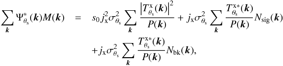 (A.2)where
the first term on the right-hand side of the equation is equal to s0 (the
amplitude of the cluster profile), the second term is the filtered Poisson fluctuations on
the signal, and the third term is the filtered background noise.
(A.2)where
the first term on the right-hand side of the equation is equal to s0 (the
amplitude of the cluster profile), the second term is the filtered Poisson fluctuations on
the signal, and the third term is the filtered background noise.
The variance of the filtered background noise can be calculated as follows: 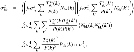 (A.3)where
we used that
(A.3)where
we used that 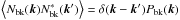 and that Pbk(k) ≈
P(k). The validity
of this approximation was confirmed empirically by checking that the power spectra of the
maps were dominated by the background.
and that Pbk(k) ≈
P(k). The validity
of this approximation was confirmed empirically by checking that the power spectra of the
maps were dominated by the background.
The variance due to the Poisson fluctuations on the signal, after passing through the
filter, can be written as 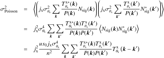 (A.4)where
the last equality comes from
(A.4)where
the last equality comes from  where
we used that
where
we used that  , Eq. (4), and the definition of the 2D Fourier
transform,
, Eq. (4), and the definition of the 2D Fourier
transform,  (A.5)where
the sum is over all the pixels in the map.
(A.5)where
the sum is over all the pixels in the map.
The double sum in Eq. (A.4) can be reduced to a single sum and calculated very efficiently by expressing it as a cross-correlation of two signals and making use of the cross-correlation theorem, as we explain next.
Let us call  ,
,
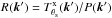 and
m =
k −
k′. Then we can express the
double sum in Eq. (A.4) as
and
m =
k −
k′. Then we can express the
double sum in Eq. (A.4) as
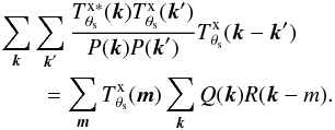 (A.6)The
second sum in the right-hand side of this equation is the cross-correlation of
Q∗ and R, evaluated at
−
m, that is,
(A.6)The
second sum in the right-hand side of this equation is the cross-correlation of
Q∗ and R, evaluated at
−
m, that is,
 (A.7)which
can be computed very efficiently by making use of the cross-correlation theorem:
(A.7)which
can be computed very efficiently by making use of the cross-correlation theorem:
 (A.8)where
ℱ denotes the Fourier
transform. Thus, the double sum in Eq. (A.4) can be calculated very quickly using the following expression:
(A.8)where
ℱ denotes the Fourier
transform. Thus, the double sum in Eq. (A.4) can be calculated very quickly using the following expression:
![Mathematical equation: \appendix \setcounter{section}{1} \begin{eqnarray*} && \sum_{{\vec k}}\sum_{{\vec k}'}\frac{T^{\rm x \ast}_{\theta_{\rm s}}({\vec k})T^{\rm x}_{\theta_{\rm s}}({\vec k}')}{P({\vec k}) P({\vec k}')} T^{\rm x}_{\theta_{\rm s}}( {\vec k}-{\vec k}') \\ && \qquad = n^2 \sum_{{\vec m}} T^{\rm x}_{\theta_{\rm s}}( {\vec m}) \left[\mathcal{F}^{-1}\left( (\mathcal{F}(R))^\ast \mathcal{F}(Q^\ast)\right)\right]^{\rm T}. \end{eqnarray*}](/articles/aa/full_html/2016/07/aa28366-16/aa28366-16-eq252.png)
Appendix B: Generation of an X-ray all-sky HEALPix map
In this section we describe how we constructed our all-sky HEALPix map using the 1378 individual RASS fields. Each RASS field covers an area of 6.4 deg× 6.4 deg (512 × 512 pixels), has a resolution of 0.75 arcmin/pixel and gives information on the number of counts in the total (0.1–2.4 keV), hard (0.5–2.0 keV) and soft (0.1–0.4 keV) bands, and the corresponding exposure time. We used the hard band information and the exposure time to build our X-ray all-sky map.
The procedure to create the all-sky map consisted of assigning each RASS pixel to the nearest HEALPix pixel (to be more precise, the sky coordinates of the center of each RASS pixel were calculated and the HEALPix pixels that contained those sky positions were assigned to them). In doing so, we came across two main difficulties: the different resolution of HEALPix maps and RASS fields, and the overlapping of contiguous RASS fields.
The Hierarchical Equal Area isoLatitude Pixelization (HEALPix) scheme (Górski et al. 2005) is based on a division of the
sphere into 12 large pixels that are further subdivided dyadically at the desired
resolution, yielding maps of Npix = 12 ×
22r pixels at resolution r, with a pixel size of
 .
For example, at Planck resolution (r = 11), we have 1.72
arcmin/pixel, while if we increase the resolution (r = 12), the pixel size is
divided by two: 0.86 arcmin/pixel. The resolution of the RASS fields is 0.75 arcmin/pixel,
which means that it does not coincide with any of the possible HEALPix resolutions. To
construct our all-sky map, we decided to work with the HEALPix resolution closest to the
RASS resolution, that is, 0.86 arcmin/pixel. Therefore, we have 1.3 RASS pixels on average
per each HEALPix pixel. To conserve the total flux of the map, we constructed the all-sky
map by summing for each HEALPix pixel the count rate (counts/second) of the corresponding
RASS pixels.
.
For example, at Planck resolution (r = 11), we have 1.72
arcmin/pixel, while if we increase the resolution (r = 12), the pixel size is
divided by two: 0.86 arcmin/pixel. The resolution of the RASS fields is 0.75 arcmin/pixel,
which means that it does not coincide with any of the possible HEALPix resolutions. To
construct our all-sky map, we decided to work with the HEALPix resolution closest to the
RASS resolution, that is, 0.86 arcmin/pixel. Therefore, we have 1.3 RASS pixels on average
per each HEALPix pixel. To conserve the total flux of the map, we constructed the all-sky
map by summing for each HEALPix pixel the count rate (counts/second) of the corresponding
RASS pixels.
A second difficulty is the fact that RASS fields overlap at least 0.23 degrees with contiguous fields. The overlapping region of two fields contains the same information, but with a different projection (so that overlapping RASS pixels do not exactly match). We decided to deal with these regions by considering only one of the fields and discarding the information from the other fields. It is worth mentioning that this choice implies that we may lose a small fraction of the flux in the borders of the overlapping regions, since the RASS pixels assigned to a HEALPix pixel in one of these borders may not cover all that HEALPix pixel area.
At this point we have a HEALPix X-ray count rate map ready to be used in the X-ray matched filter. To use this map together with the Planck multifrequency maps to jointly extract clusters using the joint X-ray-SZ MMF, we need to express all the maps in the same units. Therefore, the last step in the map construction consists of converting the X-ray map from counts/second to the equivalent ΔT/TCMB units. To do so, we need to choose a reference redshift (zref), a reference frequency (νref) and a reference temperature (Tref), as explained below, and apply the following steps:
-
1.
Convert countrate into X-ray flux: we convert counts/s (in the 0.5–2 keV band) into erg/s/cm2 (in the 0.1–2.4 keV band) using an all-sky NH map1 and interpolating in a conversion table, calculated for a temperature of Tref = 7 keV and a redshift of z = 0.3 using a mekal model and the PSPC-C response file.
-
2.
Convert X-ray flux into equivalent Y500 integrated flux: We convert the X-ray flux in the 0.1–2.4 keV band (in erg/s/cm2) into Y500 flux (in arcmin2), using the expected FX/Y500 relation. It is important to note that this expression depends on the redshift: we express our X-ray flux in the equivalent Y500 flux that we expect for clusters situated at a given redshift. Clearly, the redshifts of the clusters we are going to detect are not known in advance, so that to apply this expression we need to assume a reference redshift zref. The choice of the reference redshift will have an effect, as discussed in Sect. 4.4.
-
3.
Convert from integrated Y500 flux (in arcmin2) into y flux (adimensional), dividing the flux of each pixel by the HEALPix pixel area.
-
4.
Convert from y units into ΔT/TCMB units, using the following expression:
![Mathematical equation: \appendix \setcounter{section}{2} \begin{eqnarray} \label{eq:yDeltaTTconversion} \frac{data \left[\Delta T/T \mbox{units} \right]}{data \left[y \mbox{ units} \right]} = x \frac{{\rm e}^{x}+1}{{\rm e}^{x}-1}-4, \end{eqnarray}](/articles/aa/full_html/2016/07/aa28366-16/aa28366-16-eq269.png) (B.1)where
x =
(hν) /
(kTCMB). This step
creates a mono-frequency SZ map corresponding to the calculated flux. To apply this
conversion we need to assume a reference frequency νref for
the map, which is just a fiducial value, with no effect on the extraction algorithm.
In our case, we took νref = 1000 GHz.
(B.1)where
x =
(hν) /
(kTCMB). This step
creates a mono-frequency SZ map corresponding to the calculated flux. To apply this
conversion we need to assume a reference frequency νref for
the map, which is just a fiducial value, with no effect on the extraction algorithm.
In our case, we took νref = 1000 GHz.
Appendix C: Additional results on the gain of the X-ray-SZ MMF
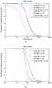 |
Fig. C.1 Percentage of RASS (top panel) and PSZ2 (bottom panel) clusters extracted with the proposed X-ray matched filter (green), the classical SZ MMF (red) and the proposed X-ray-SZ MMF (blue) whose S/N is above a certain S/N threshold, in two different redshift bins. |
In this section we provide some additional results related to the extraction of the MCXC and PSZ2 clusters using the three different filters: the classical SZ-MMF, the proposed X-ray matched filter and the proposed X-ray-SZ MMF. These results illustrate the advantage of the joint MMF, summarized in Fig. 11 for the complete samples, as a function of redshift and mass. Figure C.1 shows how the proposed joint MMF improves the detection probability of the RASS and PSZ2 clusters with respect to the single-survey filters. The samples are divided in two redshift bins to show that the gain in both regimes. Figures C.2 and C.3 compare the estimated S/N obtained for the MCXC clusters and the PSZ2 clusters using the three detection methods as a function of redshift and mass. Figure C.2 shows the individual values for each cluster, while Fig. C.3 shows the corresponding histograms. There is a S/N gain for most of the clusters, even for high redshift.
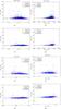 |
Fig. C.2 S/N gain of the joint extraction of the MCXC clusters (panels a)–d)) and the PSZ2 clusters (panels e)–h)) with respect to the individual SZ-only and X-ray-only extractions. The upper panels show the difference between the S/N of the joint extraction and the S/N of the SZ-only extraction, as a function of redshift a) and mass b), for the MCXC clusters. The panels in the second row show the difference between the S/N of the joint extraction and the S/N of the X-ray-only extraction, as a function of redshift c) and mass d), for the MCXC clusters. The four bottom panels are analogous to panels a)–d), but for the PSZ2 clusters. In all the cases, the S/N is defined as the estimated flux divided by the estimated background noise. Individual measurements are color-coded according to the best extraction. |
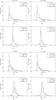 |
Fig. C.3 Histograms of the S/N gain of the joint extraction of the MCXC clusters (panels a)–d)) and the PSZ2 clusters (panels e)–h)) with respect to the individual SZ-only and X-ray-only extractions. The upper panels show the histogram of the difference between the S/N of the joint extraction and the S/N of the SZ-only extraction, on two redshift bins a) and two mass bins b), for the MCXC clusters. The panels in the second row show the histogram of the difference between the S/N of the joint extraction and the S/N of the X-ray-only extraction, on two redshift bins c) and two mass bins d), for the MCXC clusters. The four bottom panels are analogous to panels a)–d), but for the PSZ2 clusters. In all the cases, the S/N is defined as the estimated flux divided by the estimated background noise. |
Appendix D: Additional results on the photometry of the X-ray-SZ MMF
In this section, we provide additional results related to the photometry of the proposed joint MMF. In particular, we present the results from an experiment in which we injected simulated clusters in real SZ and X-ray maps and extracted them using the proposed filter, assuming their positions, sizes, and redshifts are known. In particular, we injected 1743 clusters at random positions of the sky, with characteristics (z, M500 and L500) taken from the 1743 clusters in the MCXC catalogue (Piffaretti et al. 2011), to compare with the results obtained in the extraction of the real MCXC clusters. The injection was performed following the same procedure as in Sect. 4.2, but without scatter in the FX/Y500 relation. Then, we applied the X-ray-SZ matched filter described in Sect. 4.1 at each cluster position, fixing the cluster size to the true value. To convert the X-ray map into an equivalent SZ map, we assumed the same FX/Y500 relation as used in the injection (Eq. (30)), with the real redshift of the clusters. Figure D.1 shows the extraction results for this experiment.
Main properties of the histogram in Fig. D.1.
Figure D.1a shows the extracted value of L500 for each cluster as a function of the injected value. We used the same L500 − Y500 relation as in the injection and the redshift in the catalogue to convert from the extracted Y500 value to L500. The extracted flux follows the injected flux very well, with some dispersion. The best linear fit to these data is given by y = 0.990( ± 0.004)x − 0.8( ± 2.5) × 10-4, which is very close to the unity-slope line, as shown in the figure.
Figure D.1b shows the histogram of the difference between the extracted and the injected
value, divided by the estimated standard deviation .
Some of the properties of this histogram are summarized in Table D.1. This histogram shows that there is no bias and that the estimated
error bars describe the dispersion on the results well (as 68% of the extractions fall in an interval
that is close to ±1).
The small asymmetry is produced by the fact that we are approximating y0 in Eq. (27) by its estimated value ŷ0, which yields
larger error bars for the clusters with overestimated flux and smaller error bars for the
clusters with underestimated flux.
Figures D.1c to D.1f show the difference between the extracted and the injected value,
divided by the estimated standard deviation ,
as a function of the redshift, the size, the flux, and the S/N of each cluster. The
extraction behaves correctly for all the values of these parameters, and they do not
introduce any systematic error or bias in the results.
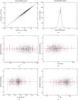 |
Fig. D.1 Photometry results of the extraction of simulated MCXC clusters (as described in Appendix D) using the proposed X-ray-SZ MMF and assuming the position, size, and redshift of the clusters are known. The six panels are analogous to those in Fig. 1. |
Appendix E: Effect of the scatter on the FX/Y500 relation
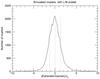 |
Fig. E.1 Histogram of the difference between the extracted and the injected L500,
divided by the estimated |
To estimate the effect of the scatter in the FX/Y500
relation, we compared the results of the simulations presented in Sect. 4.3 (see Fig. 13),
where we simulated ideal clusters covering a large area in the mass-redshift plane, with
the simulations carried out in Sect. 4.2, where we
simulated clusters with the same positions and characteristics, but adding scatter in the
L-M relation. The case with scatter shows a very good match between the extracted and the
injected flux, as in the no-scatter case, with a linear fit which is very close to the
unity-slope line (y = 1.010( ±
0.001)x − 6.3( ± 0.9) × 10-2). We also
checked that the extraction behaves correctly for all the values redshift, size, flux, and
S/N, and that these parameters do not introduce any systematic error or bias in the
results. However, we noted that the dispersion was larger than in the no-scatter case.
Figure E.1 shows the histogram of the difference
between the extracted and the injected value, divided by the estimated standard deviation
for the simulations with scatter. By comparing this to Fig. 13, we can see that the scatter in the L-M relation increases the scatter in the
extracted flux.
All Tables
All Figures
|
Fig. 1 Photometry results of the extraction of simulated MCXC clusters (as described in Sect. 2.2.1) using the proposed X-ray matched filter and assuming the position and size of the clusters are known. Top left panel: extracted versus injected L500. Individual measurements are shown as black dots. The solid blue line shows the line of zero intercept and unity slope and the dashed magenta line the best linear fit to the data. Top right panel: histogram of the difference between the extracted and the injected L500, divided by the estimated |
| In the text | |
|
Fig. 2 Photometry results of the extraction of the real MCXC clusters using the proposed X-ray matched filter and assuming the position and size of the clusters are known. The six panels are analogous to those in Fig. 1, but comparing the extracted L500 with the published L500. Individual measurements in panels a), c), d), e), and f) are shown as black and blue dots: the black dots correspond to clusters originally detected in RASS, the blue dots to serendipitous clusters. Panel b) shows three histograms that correspond to the RASS clusters (black), the serendipitous clusters (blue), and the complete MCXC sample (red). |
| In the text | |
|
Fig. 3 Percentage of MCXC clusters whose extracted S/N, using the proposed X-ray matched filter and assuming the position and size of the clusters are known, is above a given S/N threshold. Red corresponds to the complete MCXC sample, while black and blue correspond to the RASS and serendipitous subsamples, respectively. S/N is defined here as the estimated signal ŝ0 divided by the estimated background noise σθs. |
| In the text | |
|
Fig. 4 Photometry results of the extraction of the ESZ-XMM clusters using the proposed X-ray matched filter with the average cluster profile and assuming the position and size of the clusters are known. Top left panel: extracted versus published L500. The error bars correspond to the estimated |
| In the text | |
|
Fig. 5 Photometry results of the extraction of the ESZ-XMM clusters using the proposed X-ray matched filter with the individual cluster profiles and assuming the position and size of the clusters are known. The four panels are analogous to those in Fig. 4. The top right panel includes in this case two histograms, one corresponding to the whole ESZ-XMM sample (black) and another corresponding to the ESZ-XMM-A subsample (red), which includes the clusters well within the XMM-Newton field of view. |
| In the text | |
|
Fig. 6 Histogram of the difference between the extracted and the published L500, divided by the standard deviation after correcting for the effect of the profile mismatch (σcorr, scaled to L500 units) for the MCXC clusters extracted with the proposed X-ray matched filter using the average profile and assuming the position and size of the clusters are known. Red corresponds to the complete MCXC sample, while black and blue correspond to the RASS and serendipitous subsamples, respectively. For each color, the central vertical line shows the median value, whereas the other two vertical lines indicate the region inside which 68% of the clusters lie. |
| In the text | |
|
Fig. 7 Top panels: S/N of the clusters extracted with the proposed X-ray matched filter (left panel), the classical SZ MMF (middle panel), and the proposed X-ray-SZ MMF (right panel), averaged in different mass and redshift bins. White lines indicate smoothed isocontours corresponding to a S/N of 3, 4, and 5. White bins indicate a S/N greater than 20. Bottom panels: average difference between the S/N obtained with the proposed X-ray-SZ MMF and the S/N obtained with SZ MMF (left panel) and the X-ray MF (right panel). White lines indicate smoothed isocontours corresponding to a difference in S/N of 1, 2, and 3. White bins indicate a difference in S/N greater than 10. |
| In the text | |
|
Fig. 8 Estimated completeness of the proposed X-ray matched filter (left panels), the classical SZ MMF (middle panels) and the proposed X-ray-SZ MMF (right panels) for a S/N threshold of 3.0 (top panels) and 4.5 (bottom panels), in different redshift-mass bins. |
| In the text | |
|
Fig. 9 Estimated completeness of the proposed X-ray matched filter (dashed lines), the classical SZ MMF (dotted lines), and the proposed X-ray-SZ MMF (solid lines) as a function of redshift for a S/N threshold of 3.0 (left panel) and 4.5 (right panel). The different colors correspond to different mass bins, as indicated in the legend. |
| In the text | |
|
Fig. 10 MCXC and PSZ2 cluster samples in the mass-redshift plane. The MCXC sample is divided into RASS and serendipitous subsamples. |
| In the text | |
|
Fig. 11 Percentage of MCXC (top panel) and PSZ2 (bottom panel) clusters extracted with the proposed X-ray matched filter (green), the classical SZ MMF (red), and the proposed X-ray-SZ MMF (blue) whose S/N is above a certain S/N threshold. In the top panel, the complete MCXC sample (solid lines) is divided into RASS (dotted lines) and serendipitous clusters (dashed lines). |
| In the text | |
|
Fig. 12 S/N maps obtained in the extraction of cluster PSZ2 G156.26+59.64 using the SZ-MMF (left) and the X-ray-SZ MMF (right). The S/N at the cluster position improves from 5.38 to 11.92. The angular size of the images is 3°. The cluster redshift is z = 0.59. We have masked an X-ray source to the bottom-left of the cluster. |
| In the text | |
|
Fig. 13 Histogram of the difference between the extracted and the injected L500, divided by the estimated |
| In the text | |
|
Fig. 14 Photometry results of the extraction of the MCXC clusters using the proposed X-ray-SZ filter with the average cluster profile and assuming the position, size, and redshift of the clusters are known. The top left panel is analogous to the top left panel of Fig. 2, and its subpanel shows the histogram of the difference between the extracted and the published L500, divided by the estimated |
| In the text | |
|
Fig. 15 Photometry results of the extraction of the PSZ2 clusters using the proposed X-ray-SZ filter with the average cluster profile and assuming the position, size, and redshift of the clusters are known. The six panels are analogous to those in Fig. 14, with panel e showing the difference between the extracted and the published L500, divided by the corrected standard deviation σcorrJ as a function of the mass of each cluster instead of as a function of the flux as in Fig. 14e. |
| In the text | |
|
Fig. 16 Expected values of the extracted flux (left panel) and the estimated S/N (right panel) when an incorrect FX/Y500 relation is assumed. The figure shows the ratio with respect to the expected value corresponding to the true relation as a function of the relative contribution of the X-ray and SZ background noises ω (low ω values represent better SZ maps and high ω values correspond to a better X-ray map). Different values of a = (FX/Y500)assumed/ (FX/Y500)true are shown in different colors, according to the legend. |
| In the text | |
|
Fig. 17 Histogram of the relative contribution of the X-ray and SZ background noises ω for the RASS and Planck maps. |
| In the text | |
|
Fig. 18 Percentage of simulated clusters (as described in Sect. 4.4) whose extracted S/N, using the proposed X-ray matched filter and assuming the position, size, and redshift of the clusters are known, is above a given S/N threshold. The different colors correspond to different normalizations of the FX/Y500 relation assumed for the extraction, as indicated in the legend. |
| In the text | |
|
Fig. 19 Histogram of the difference between the extracted and the injected L500, divided by the estimated |
| In the text | |
|
Fig. C.1 Percentage of RASS (top panel) and PSZ2 (bottom panel) clusters extracted with the proposed X-ray matched filter (green), the classical SZ MMF (red) and the proposed X-ray-SZ MMF (blue) whose S/N is above a certain S/N threshold, in two different redshift bins. |
| In the text | |
|
Fig. C.2 S/N gain of the joint extraction of the MCXC clusters (panels a)–d)) and the PSZ2 clusters (panels e)–h)) with respect to the individual SZ-only and X-ray-only extractions. The upper panels show the difference between the S/N of the joint extraction and the S/N of the SZ-only extraction, as a function of redshift a) and mass b), for the MCXC clusters. The panels in the second row show the difference between the S/N of the joint extraction and the S/N of the X-ray-only extraction, as a function of redshift c) and mass d), for the MCXC clusters. The four bottom panels are analogous to panels a)–d), but for the PSZ2 clusters. In all the cases, the S/N is defined as the estimated flux divided by the estimated background noise. Individual measurements are color-coded according to the best extraction. |
| In the text | |
|
Fig. C.3 Histograms of the S/N gain of the joint extraction of the MCXC clusters (panels a)–d)) and the PSZ2 clusters (panels e)–h)) with respect to the individual SZ-only and X-ray-only extractions. The upper panels show the histogram of the difference between the S/N of the joint extraction and the S/N of the SZ-only extraction, on two redshift bins a) and two mass bins b), for the MCXC clusters. The panels in the second row show the histogram of the difference between the S/N of the joint extraction and the S/N of the X-ray-only extraction, on two redshift bins c) and two mass bins d), for the MCXC clusters. The four bottom panels are analogous to panels a)–d), but for the PSZ2 clusters. In all the cases, the S/N is defined as the estimated flux divided by the estimated background noise. |
| In the text | |
|
Fig. D.1 Photometry results of the extraction of simulated MCXC clusters (as described in Appendix D) using the proposed X-ray-SZ MMF and assuming the position, size, and redshift of the clusters are known. The six panels are analogous to those in Fig. 1. |
| In the text | |
|
Fig. E.1 Histogram of the difference between the extracted and the injected L500,
divided by the estimated |
| In the text | |
Current usage metrics show cumulative count of Article Views (full-text article views including HTML views, PDF and ePub downloads, according to the available data) and Abstracts Views on Vision4Press platform.
Data correspond to usage on the plateform after 2015. The current usage metrics is available 48-96 hours after online publication and is updated daily on week days.
Initial download of the metrics may take a while.