| Issue |
A&A
Volume 590, June 2016
|
|
|---|---|---|
| Article Number | A127 | |
| Number of page(s) | 56 | |
| Section | Interstellar and circumstellar matter | |
| DOI | https://doi.org/10.1051/0004-6361/201527867 | |
| Published online | 27 May 2016 | |
Resolving the extended atmosphere and the inner wind of Mira (o Ceti) with long ALMA baselines
1
Max-Planck-Institut für Radioastronomie,
Auf dem Hügel 69,
53121
Bonn,
Germany
e-mail: This email address is being protected from spambots. You need JavaScript enabled to view it.
; This email address is being protected from spambots. You need JavaScript enabled to view it.
; This email address is being protected from spambots. You need JavaScript enabled to view it.
2
ESO, Alonso de Córdova 3107, Vitacura, Casilla 19001,
Santiago,
Chile
e-mail:
This email address is being protected from spambots. You need JavaScript enabled to view it.
Received: 1 December 2015
Accepted: 9 March 2016
Abstract
Context. High angular resolution (sub)millimetre observations of asymptotic giant branch (AGB) stars, now possible with the Atacama Large Millimeter/submillimeter Array (ALMA), allow direct imaging of these objects’ photospheres. The physical properties of the molecular material around these regions, which until now has only been studied by imaging of maser emission and spatially unresolved absorption spectroscopy, can be probed with radiative transfer modelling and compared to hydrodynamical model predictions. The prototypical Mira variable, o Cet (Mira), was observed as a Science Verification target in the 2014 ALMA Long Baseline Campaign, offering the first opportunity to study these physical conditions in detail.
Aims. With the longest baseline of 15 km, ALMA produces clearly resolved images of the continuum and molecular line emission/absorption at an angular resolution of ~30 mas at 220 GHz. Models are constructed for Mira’s extended atmosphere to investigate the physics and molecular abundances therein.
Methods. We imaged the data of 28SiO ν= 0, 2J = 5−4 and H2O v2 = 1JKa,Kc = 55,0−64,3 transitions and extracted spectra from various lines of sight towards Mira’s extended atmosphere. In the course of imaging the emission/absorption, we encountered ambiguities in the resulting images and spectra that appear to be related to the performance of the CLEAN algorithm when applied to a combination of extended emission, and compact emission and absorption. We addressed these issues by a series of tests and simulations. We derived the gas density, kinetic temperature, molecular abundance, and outflow/infall velocities in Mira’s extended atmosphere by modelling the SiO and H2O lines.
Results. We resolve Mira’s millimetre continuum emission and our data are consistent with a radio photosphere with a brightness temperature of 2611 ± 51 K. In agreement with recent results obtained with the Very Large Array, we do not confirm the existence of a compact region (<5 mas) of enhanced brightness. Our modelling shows that SiO gas starts to deplete beyond 4 R⋆ and at a kinetic temperature of ≲ 600 K. The inner dust shells are probably composed of grain types other than pure silicates. During this ALMA observation, Mira’s atmosphere generally exhibited infall motion with a shock front of velocity ≲ 12 km s-1 outside the radio photosphere. Despite the chaotic nature of Mira’s atmosphere, the structures predicted by the hydrodynamical model, codex, can reproduce the observed spectra in astonishing detail, while some other models fail when confronted with the new data.
Conclusions. For the first time, millimetre-wavelength molecular absorption against the stellar continuum has been clearly imaged. Combined with radiative transfer modelling, the ALMA data successfully demonstrates the ability to reveal the physical conditions of the extended atmospheres and inner winds of AGB stars in unprecedented detail. Long-term monitoring of oxygen-rich evolved stars will be the key to understanding the unsolved problem of dust condensation and the wind-driving mechanism.
Key words: radiative transfer / stars: atmospheres / stars: winds, outflows / stars: AGB and post-AGB / stars: individual: oCet / radio continuum: stars
Member of the International Max Planck Research School (IMPRS) for Astronomy and Astrophysics at the Universities of Bonn and Cologne.
© ESO, 2016
1. Introduction
Mira A (o Ceti; Mira) is an oxygen-rich, long-period variable star on the asymptotic giant branch (AGB). Together with Mira B (VZ Ceti), which is possibly a white dwarf (Sokoloski & Bildsten 2010), they form the symbiotic binary system Mira AB. Mira A is the prototype of Mira variables. Its period of visual brightness variation is about 332 days and the visual V-band magnitude of the star varies by up to about 8.1 mag (a factor of >1700) in each cycle (based on the data in the American Association of Variable Star Observers, AAVSO, International Database). The large variation in the visual magnitude is caused by a combined effect of stellar pulsation and variable opacity of metal oxides whose abundance changes with the effective temperature of the star (Reid & Goldston 2002). The distance of the Mira AB system was estimated to be 110 ± 9 pc (Haniff et al. 1995), which is based on the period-luminosity relation derived by Feast et al. (1989), the infrared K-band magnitude from Robertson & Feast (1981), and the period of the visual V variation from the GCVS (Kholopov 1987). Throughout the article we adopt this value, which is roughly consistent with the revised Hipparcos value of 92 ± 10 pc (van Leeuwen 2007).
Observed spectral lines in ALMA Band 6.
Traditionally, AGB star atmospheres have been probed by molecular absorption spectroscopy, which delivers spatially unresolved line of sight information. Examples include the detection of the near-infrared H2O absorption band from the warm molecular forming layer (known as the MOLsphere) around M giant stars and Mira variables with the Infrared Space Observatory (ISO) (e.g. Tsuji et al. 1997; Woitke et al. 1999; Tsuji 2000). In addition, mid-infrared interferometry with the Very Large Telescope Interferometer (VLTI) can also probe the molecular layers and dust shells around these stars (e.g. Ohnaka et al. 2005; Karovicova et al. 2011). Maser emission from SiO and/or H2O in the extended atmospheres of Mira variables has been imaged (see e.g. Cotton et al. 2004; and Perrin et al. 2015 with the Very Long Baseline Array (VLBA); and Reid & Menten 2007 with the Very Large Array (VLA)).
In order to test the predictions of existing hydrodynamical models for the extended atmospheres of Mira variables, which typically has a radius of only a few R⋆ (a few tens of milli-arcseconds for Mira A), high angular and spectral resolution observations of the molecular emission and absorption from these regions are mandatory. The Atacama Large Millimeter/submillimeter Array (ALMA) with long baselines thus allows us to reach the required angular resolution at high sensitivity and to study the detailed kinematics of the innermost envelope of Mira A. Observations of radio and (sub)millimetre wavelength molecular line emission/absorption, in particular the rotational transitions not exhibiting strong masers, can be used to compare and test the predicted structures of the extended atmospheres by hydrodynamical models. Through modelling the radiative transfer of the transition lines with the predicted atmospheric structures used as the inputs, synthesised spectra can be produced and compared to the observed ones.
In this article, we present the new ALMA observations of the Mira AB system, which was selected as one of the Science Verification (SV) targets in the 2014 ALMA Long Baseline Campaign to demonstrate the high angular resolution capability of ALMA (ALMA Partnership et al. 2015). Based on the visual magnitude data reported by the AAVSO, the stellar phase of Mira A is ~0.45 at the time of this observation, and we adopt this phase throughout the article. In Sect. 2, we describe the SV observation of Mira AB and the data processing. In Sect. 3, we present the results including the radio continuum data of Mira A and B in the SV dataset, and the images and spectra of the SiO and H2O lines from Mira A as covered in the observations. In Sect. 4, we present our radiative transfer modelling results of the SiO and H2O spectra of Mira A. In Sect. 5, we discuss the implications of our modelling results for our understanding of Mira A’s extended atmosphere, including the structures, dust condensation process, shock dissipation, and the kinematics and compare these values with predictions from hydrodynamical models.
2. Observations and data processing
The Mira AB system was observed with ALMA on 2014 October 17 and 25 (ALMA Band 3) and on 2014 October 29 and November 1 (ALMA Band 6) as part of the 2014 ALMA Long Baseline Campaign Science Verification with the longest baseline of 15.24 km. (ALMA Partnership et al. 2015). By referring to the AAVSO visual data for Mira, we find that the ALMA observations took place between the visual phases 0.42 (2014 Oct. 17) and 0.47 (2014 Nov. 01)1.
The shortest baselines (and the maximum number of antennae) in the observations of Bands 3 and 6 are 29.07 m (38) and 15.23 m (39), respectively. The maximum recoverable scales2 of the SiO lines in Bands 3 and 6 are therefore  and
and  , respectively, and that of the H2O v2 = 1 line in Band 6 is
  . In Band 3, three continuum windows at 88.2, 98.2, and 100.2 GHz were observed, in addition to four spectral line windows of 58.6 MHz bandwidth around the transitions of 28SiO ν= 0,1,2J = 2−1 and 29SiO ν= 0J = 2−1. The channel width of the spectral windows is 61.0 kHz (~0.21 km s-1). In Band 6, a continuum window at 229.6 GHz together with six spectral line windows of 117.2 MHz bandwidth around 28SiO ν= 0,1,2J = 5−4, 29SiO ν= 0J = 5−4, H2O v2 = 1JKa,Kc = 55,0−64,3, and the H30α recombination line were observed. The channel width of the four SiO windows is 122.1 kHz (~0.17 km s-1) and that of the H2O and H recombination line windows is 61.0 kHz (~0.08 km s-1). Table 1 summarises the observed spectral lines and their parameters.
The SV data was calibrated by staff members of the Joint ALMA Observatory (JAO) and the ALMA Regional Centres (ARCs), with the Common Astronomy Software Applications (CASA; McMullin et al. 2007) package3 version 4.2.2. Detailed calibration scripts, preliminarily calibrated data products (i.e. without self-calibration), and self-calibration solutions for both continuum and spectral line data are available at the ALMA Science Portal4. Self-calibration solutions were derived from the continuum data for the continuum data itself and from the strongest spectral channels of the 28SiO ν= 1 data, which exhibits strong maser emission for the spectral line data. We downloaded the self-calibration solutions from the ALMA Science Portal and applied them to the preliminarily calibrated data, and then imaged the continuum and spectral line data. We used CASA version 4.2.2 for the self-calibration and imaging (except for the image binning task as mentioned below), and the Miriad package5 for our continuum analysis in Sect. 3.1 and Appendix A (Sault et al. 1995).
We determined the centre of Mira A’s continuum emission to be at  by fitting its image, produced from the visibility data before self-calibration, in the 229.6 GHz continuum windows (i.e. spectral windows spw= 0,7 in the SV dataset). We adopt these coordinates as the absolute position of Mira A. The position and proper motion of Mira A in the Hipparcos Catalogue are
 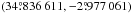 at the Julian epoch 1991.25 and (9.33 ± 1.99,−237.36 ± 1.58) mas yr-1, respectively (van Leeuwen 2007). At the epoch of the ALMA SV observation, ~2014.83 (JD 2 456 959.6 and JD 2 456 962.7), the expected coordinates of Mira A due to proper motion should be
  . So the observed absolute position of Mira A is within 2σ of the predicted position of the Hipparcos Catalogue.
We then produced two sets of spectral line images, with and without subtraction of the continuum. The continuum was subtracted with the uvcontsub task in CASA by fitting a linear polynomial to the real and imaginary parts of the visibility data of the line-free (i.e. continuum-only) channels in each spectral window. Our selection of the line-free channels was slightly different from that in the example imaging script provided along with the SV data6.
The spectral line image data cubes of the SiO and H2O lines in ALMA Band 6 were created by the image deconvolution task clean in CASA. The task performs an inverse Fourier transform to the visibility data (uv-data) and creates a raw image data cube (the DIRTY image), then deconvolves the ALMA point-spread function from each frequency plane of the image with the Clark image deconvolution algorithm (Högbom 1974; Clark 1980; the CLEAN process). The product of image deconvolution for each frequency is a set of point sources (the CLEAN component models) which, in aggregate, reproduce the same input DIRTY image when convolving with the array’s point-spread function. The task finally restores the CLEAN component models with a restoring beam (the CLEAN beam) of parameters either determined from fitting the point-spread function (taking its full width at half maximum, FWHM) or specified by the user. The local standard of rest (LSR) velocities covered by the image cubes range from 26.7 km s-1 to 66.7 km s-1, centred at the systemic (centre of mass) LSR velocity of 46.7 km s-1, which corresponds to 57.0 km s-1 in the heliocentric rest frame. We determined the systemic velocity from the mid-point of the total velocity ranges of the entire line-emitting/absorbing region, assuming that the global infall or expansion motions at the extreme velocities are symmetric about the stellar systemic velocity. We weighted the visibilities with a robust (Briggs) parameter of ℛBriggs = 0.5 and CLEANed the images down to a threshold of ~2−3 mJy beam-1, which is about 1.5 times the rms noise level. We restored the images with a circular beam of FWHM  for the 28SiO and 29SiO lines, and of FWHM
  for the H2O v2 = 1 line. The FWHM of the beams are the geometric means of the major- and minor-axes of the elliptical point-spread functions fitted by the clean task.
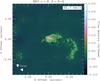 |
Fig. 1 Map of SiO ν= 0J = 5−4 (with the continuum) at the channel of the systemic velocity (46.7 km s-1) with a channel width of 1.0 km s-1. The positions of Mira A (o Ceti; cyan cross) and Mira B (VZ Ceti; yellow cross) are indicated in the image. The horizontal and vertical axes are the relative offsets (arcsec) in the directions of right ascension (X) and declination (Y), respectively, with respect to the continuum centre of Mira A. The white box centred at the fitted position of Mira A indicates the |

At 220 GHz, the primary beam FWHM of the 12 m array is about 28″, which is much larger than the size of the line emission/absorption, and therefore no primary beam correction is needed. Figure 1 is the only primary beam-corrected image in this article, which shows remote emission in the vibrational ground state 28SiO up to a distance of ~3″. There is no significant difference in the flux of detectable emission from the image without primary beam correction.
Photospheric parameters from fitting the continuum visibility data, using the uvfit task in the Miriad software, of Mira A and B in the continuum window at 229.6 GHz of ALMA Band 6.
The spectral line channel maps presented in Sect. 3.2 and Appendix C are further binned with the image binning task imrebin (new from version 4.3.0) in CASA version 4.4.0. We use Python to generate plots with the aid of the matplotlib plotting library (version 1.4.3; Hunter 2007), the PyFITS module (version 3.3), and the Kapteyn Package7 (version 2.3; Terlouw & Vogelaar 2015).
The cell size and total size of the images are  and 15″ × 15″, respectively. Figure 1 shows the map of the SiO ν= 0J = 5−4 line at the systemic velocity channel over a
  region centred at Mira A. As shown in this figure, there is remote, arc-like emission extending up to about 3 arcsec from the star between the LSR velocities of 43.7 km s-1 and 49.7 km s-1.
Moreover, we use the images without continuum subtraction for our spectral line modelling (Sect. 3.3 and later), instead of the continuum-subtracted images as in the reference images in the ALMA Science Portal. As a result, our images only contain emission from spectral line and/or the radio continuum from Mira A and B throughout without any real negative signals. As we will explain in further detail in Appendix B, we find spurious “bumps” in the absorption profiles of continuum-subtracted spectra. We believe that the image deconvolution of the strong line emission surrounding Mira’s radio photosphere may have impaired the deconvolution of the region showing line absorption against the background continuum. The images (and hence the spectra) deconvolved without continuum subtracted should better represent the real emission and absorption of the SiO and H2O lines.
3. Results
3.1. Continuum
Matthews et al. (2015) and Vlemmings et al. (2015) have independently analysed the continuum data of the Mira AB system in both ALMA Bands 3 (96 GHz) and 6 (229 GHz) of this SV dataset. Additionally, Matthews et al. (2015) include the continuum data from their Q-band (46 GHz) observation with the Karl G. Jansky VLA in 2014. Vlemmings et al. (2015) also include the continuum data from ALMA Band 7 (338 GHz); some of these results have been reported by Ramstedt et al. (2014). From this SV dataset, both Matthews et al. (2015) and Vlemmings et al. (2015) found that the visibilities of Mira A in the continuum of Band 6 can be better fitted with a two-component model consisting of an elliptical uniform disk plus an additional Gaussian component than with a single-component model. Moreover, Vlemmings et al. (2015) found that the additional Gaussian component is a compact, bright hotspot with a FWHM of ~4.7 mas and a brightness temperature of ~10 000 K.
We conducted a similar analysis of the continuum data of Mira A and B as these authors for the Band 6 data. From the continuum map, the total flux of Mira A is 149.70 ± 0.04 mJy and that of Mira B is 11.19 ± 0.04 mJy. In our model fitting, the elliptical uniform disk component for Mira A has a size of about (51.2 ± 0.1) mas × (41.0 ± 0.1) mas, PA = −45.0° ± 0.5° and a flux of S229.6 GHz = 102 ± 9 mJy. This corresponds to a brightness temperature of 1630 ± 175 K. For the additional Gaussian component of Mira A, the fitted flux is about 47 ± 9 mJy and its FWHM is about (26.4 ± 0.2) mas × (22.4 ± 0.2) mas, PA = 34.0° ± 1.7°, which is much larger than the size of the purported 4.7 mas hotspot. The brightness temperature of this Gaussian component corresponds to 1856 ± 419 K, which is much smaller than 10 000 K. Our elliptical Gaussian model for Mira B has a FWHM of about (25.5 ± 0.3) mas × (22.5 ± 0.3) mas, PA = 72.7° ± 3.6° and a flux of about (11.3 ± 0.5) mJy. In general, our results are consistent with those reported by Matthews et al. (2015). However, we did not find any evidence of the compact hotspot or reproduce the similar results of the visibility fitting as reported by Vlemmings et al. (2015). We present our detailed continuum analysis of the visibility data in Appendix A.
In this section, we only present our model fitting results using a single model component for Mira, i.e. an elliptical uniform disk or an elliptical Gaussian, but not both. Table 2 shows the results of our single-component fitting in the continuum window centred at 229.6 GHz. The brightness temperature of the uniform disk model of Mira A is found to be 2611 ± 51 K.
In addition, we created continuum images by integrating all the line-free channels in each of the four SiO and one H2O spectral line windows. By calculating the total flux, Sν, from Mira A within a  -radius circle (which safely includes all possible continuum emission from Mira A, but does not contain any emission from Mira B) at respective frequencies, ν, we derive an independent spectral index (using the spectral line windows in Band 6 only) of 1.82 ± 0.33, which is consistent with the value (1.86) derived by Reid & Menten (1997a).
3.2. Images
Figure 1 shows the map of the SiO ν= 0J = 5−4 transition in the LSR velocity of 46.7 km s-1, which is the systemic (centre of mass) velocity of Mira A, over a  box centred at Mira A. The position of Mira B,
  , determined by fitting its image produced from the uv-data before self-calibration, is also indicated on the map. To the west of Mira A, the SiO vibrational ground state emission extends to a larger projected radial distance than other directions. This emission feature emerges from the west and north-west of Mira A and appears as an arc-like feature, which turns south at around 2″ west of the star and reaches a maximum projected distance of ~3″.
As we explain in Appendix B, there are spurious bumps in the spectra extracted from the line of sight towards the continuum of Mira in the maps produced from the data continuum-subtracted before imaging. Since we are more confident in the quality of the image deconvolution without the subtraction of the continuum, we extract the spectra from the maps retaining the continuum (full data maps) for our radiative transfer modelling in Sects. 3.3 and later. These full data maps are presented in Appendix C. In this section, we only show the maps that are first imaged with the continuum, and then continuum-subtracted with the CASA task imcontsub. Such post-imaging continuum subtraction can avoid the spurious features seen in pre-imaging continuum-subtracted images (and also the spectra).
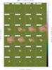 |
Fig. 2 Channel maps of post-imaging continuum-subtracted SiO ν= 0J = 5−4 from LSR velocity 35.7 km s-1 to 58.7 km s-1, with a channel width of 1.0 km s-1. The systemic velocity is 46.7 km s-1. The horizontal and vertical axes indicate the relative offsets (arcsec) in the directions of right ascension (X) and declination (Y), respectively, with respect to the fitted absolute position of Mira A. The white contours represent 6, 12, 18, 24, 48, and 72σ and yellow contours represent −60, −36, and −6σ, where σ = 0.80 mJy beam-1 is the map rms noise. The circular restoring beam of |

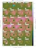 |
Fig. 3 Same as Fig. 2 for the zoomed ( |

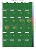 |
Fig. 4 Same as Fig. 2 for the channel maps of post-imaging continuum-subtracted 29SiO ν= 0J = 5−4. The white contours represent 6, 12, 24, 48, 96, and 144σ and yellow contours represent −72, −54, −36, and −6σ, where σ = 0.65 mJy beam-1 is the map rms noise. |
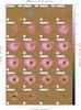 |
Fig. 5 Same as Fig. 2 for the zoomed ( |
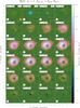 |
Fig. 6 Same as Fig. 2 for the zoomed ( |
Figure 2 shows the continuum-subtracted channel maps of the SiO ν= 0J = 5−4 transition in the LSR velocity range of 35.7−58.7 km s-1 over a  box centred at Mira A (Mira hereafter). Contour lines at the −36, −6, 6, 12, 24, 48, and 72σ levels, where σ = 0.80 mJy beam-1, are drawn to indicate the region with significant line absorption (yellow contours for negative signals) or emission (white contours for positive signals).
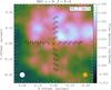 |
Fig. 7 Map of SiO ν= 0J = 5−4 (with the continuum) at the channel of the systemic velocity (46.7 km s-1) with a channel width of 1 km s-1. The centre of Mira’s continuum is indicated by a black cross. Orange contours represent 10%, 30%, 50%, 70%, and 90% of the peak continuum flux (73.4 mJy beam-1). The black plus signs (+) indicate the positions at which SiO and H2O spectra are sampled and modelled in Sect. 4. The sampling positions are separated by 32 mas along each arm of this array of points. The circular restoring beam of |
Figure 3 shows the same channel maps as Fig. 2, but zoomed in to show the inner  region around Mira. Overall, the emission of the vibrational ground state SiO line in the inner winds of Mira (
 ) appears to be spherically symmetric, although we find significant inhomogeneities with stronger emission from clumps that are localised in relatively small regions and which stretch over limited velocity ranges.
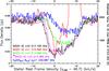 |
Fig. 8 Spectral lines in ALMA Band 6 extracted from the line of sight towards the centre of Mira’s continuum. The SiO ν= 1J = 5−4 transition (in red) shows intense maser emission around + 10 km s-1, with the peak flux density of 1.73 Jy at + 8.8 km s-1. The maser spectrum above 0.10 Jy is not shown in this figure. |
As shown in Fig. 4, the absorption and emission in the J = 5−4 transition of the vibrational ground state of the 29SiO isotopologue appears to have a very similar extent to that observed in the analogous line to the main isotope of SiO. On larger scales, the 29SiO emission also appears to extend to the west of Mira, while its intensity falls off much more rapidly with increasing radius and no significant emission is seen beyond ~0.5″. This is expected because the isotopic ratio of 28Si/29Si in oxygen-rich giants is ≳ 13 (e.g. Tsuji et al. 1994; Decin et al. 2010; Ohnaka 2014). The 29SiO emission within  also exhibits (1) general spherical symmetry and (2) localised, clumpy structures with more intense emission. While the maps in both isotopologues have a similar overall morphology, the peaks in the 29SiO emission do not all coincide with the 28SiO peaks.
Figures 5 and 6 show the continuum-subtracted maps of the SiO ν= 2J = 5−4 and H2O v2 = 1JKa,Kc = 55,0−64,3 lines, respectively. Since the emission of these two lines is more smoothly distributed than that in the vibrational ground state SiO and 29SiO lines, we can clearly see ring-like emission structures around the line absorption against Mira’s continuum in the velocity channels around the systemic velocity (46.7 km s-1). In most velocity channels, the emission from both lines are confined well within  of the centre of the continuum, and there is no remote emission beyond
  as in the ground state SiO lines.
Close to the systemic velocity, there is a clump at about 0 05 to the east of Mira which strongly emits in both the SiO ν= 2 and H2O v2 = 1 lines. The brightness temperatures of the SiO ν= 2 and H2O v2 = 1 emission are ~600 K and ~1000 K, respectively. However, this eastern clump is not prominent in the vibrational ground state SiO and 29SiO lines, which have very low excitation energies (i.e. the upper-state energy, Eup). This clump therefore probably contains shock-heated gas at a high kinetic temperature (Tkin ≳ 1000 K). On the other hand, the intensely emitting clumps in the ground state of SiO or 29SiO lines do not appear in the highly excited SiO ν= 2 and H2O v2 = 1 lines, which have excitation energies of Eup/k ≳ 3500 K.
3.3. Spectra
We have extracted the SiO and H2O spectra from the centre of Mira’s continuum, and from an array of positions at radii 0.̋032, 0.̋064, 0.̋096, 0.̋128, and 0.̋160 from the centre, along the legs at PA = 0°, 90°, 180°, and 270°. The positions are shown in Fig. 7, which is the map of SiO ν= 0J = 5−4, without subtraction of the continuum, in the channel of the stellar systemic velocity (vLSR = 46.7 km s-1). The full set of the spectra are presented along with the modelling results in Sect. 4. Because the inner envelope around Mira is partially filled with intense clumpy emission, we did not compute the azimuthally averaged spectra in order to avoid the averaged spectra from being contaminated by isolated intense emission and to obtain a more representative view of the general physical conditions of the envelope.
Figure 8 shows the spectra of various lines in ALMA Band 6 extracted from the centre of the continuum. As we did not subtract the continuum from the data, the flat emission towards the low- and high-velocity ends of the spectra represents the flux from the radio continuum of Mira near the frequencies of the respective spectral lines. In Appendix B, we show the spectra with the continuum subtracted (in the visibility data) before imaging.
The SiO ν= 1J = 5−4 transition shows strong maser emission across a wide range of LSR velocities, which introduces sharp spikes in its spectrum. For other lines which do not show strong maser emission (i.e. all except SiO ν= 1), absorption against the continuum ranges between the offset velocity (relative to the stellar LSR velocity) of approximately −4 km s-1 and + 14 km s-1. The absorption is in general redshifted relative to the systemic velocity. This indicates that the bulk of the material in the inner envelope is infalling towards Mira during the ALMA SV observation (near stellar phase 0.45). Infall motion at phase 0.45 is expected for another oxygen-rich Mira variable, W Hya, based on the detailed modelling of the CO Δν = 3 line profiles, as observed by Lebzelter et al. (2005), presented in the paper of Nowotny et al. (2010). The CO Δν = 3 lines probe the pulsation-dominated layers of the atmospheres of Mira variables, and therefore the radial velocity variation of these lines indicate the infall or expansion velocities of the global motion of the extended atmospheres below the dust formation (and circumstellar wind acceleration) regions (e.g. Hinkle et al. 1982; Nowotny et al. 2005a).
The spectra of 28SiO ν= 0J = 5−4 and 29SiO ν= 0J = 5−4 appear to be virtually identical. From the similarity of the line profiles and considering the high expected isotopic ratio of 28Si/29Si (≳13), the vibrational ground state 28SiO and 29SiO lines we see in Fig. 8 are likely to be both very optically thick (saturated) and thermalised.
In Fig. 8, we can also see trends in the width and depth of the absorption profiles with excitation. The vibrationally excited SiO ν= 2 and H2O v2 = 1 lines show narrower and shallower absorption than the two ground state SiO lines. This suggests that the vibrationally excited energy levels are less readily populated than the ground state levels, and hence the kinetic temperature of the bulk of the infalling material should be much lower than 3500 K, which corresponds to the excitation energies of SiO ν= 2 and H2O v2 = 1 lines. This also explains the small radial extent of these two lines as shown in the channel maps because the kinetic temperature (and hence the excitation) in general falls off with the radial distance from the star. Because the SiO ν= 2 and H2O v2 = 1 lines have very similar excitation energy (Eup/k ~ 3500 K), the difference in their line profiles is probably due to differences in the molecular abundance and molecular parameters such as the (de-)excitation rate coefficients.
There are two features in the spectra that strongly constrain our modelling in Sect. 4. The first is the small blueshifted emission feature at the offset velocities between −10 and −3 km s-1. The size of the synthesised beam under robust weighting (ℛBriggs = 0.5) is about  , which is comparable to that of the disk of the continuum emission (with minor axis about
  ). Hence, some emission from the hottest inner layers of the envelope just outside the edge of the continuum disk is expected to “leak” into the beam. Since the innermost envelope shows global infall kinematics, the flux leakage should appear as excess blueshifted emission, i.e. an inverse P Cygni profile. We have also checked the spectra at different offset positions (some of which are modelled in Sect. 4) and found that over the same blueshifted velocity range, the excess emission becomes more prominent as the continuum level decreases towards outer radial distances. For the H2O transition, we also find a much weaker emission component near the offset velocity of −3 km s-1, and a similar check at different offset positions also indicates that the component is likely to be real.
The other feature is presented by the redshifted wings in the offset velocity range between + 10 and + 14 km s-1 of the 28SiO ν= 0 and 2 and the 29SiO ν= 0 lines, which do not show strong maser emission. As shown in Fig. 8, the redshifted part of the absorption profiles of all these lines appears to be nearly identical. The lines could be in the optically thin regime only if the isotopic ratio of 28SiO/29SiO is close to unity, which is not expected. So we believe that all the lines are in the optically thick regime in this velocity range. The brightness temperatures of the redshifted wings thus give an indication of the kinetic temperature of the coolest gas around the corresponding infall velocities.
4. Radiative transfer modelling
We modelled the H2O and SiO spectra with the radiative transfer code ratran8 (Hogerheijde & van der Tak 2000). The public version of the code accepts 1D input models only. Despite the clumpy structures of the inner envelope, we find that the line spectra exhibit general spherical symmetry within  and therefore 1D modelling is applicable. Since the ALMA SV observations only provide a snapshot of Mira’s extended atmosphere in its highly variable pulsation cycles, and the hydrodynamical models that we compare and discuss in Sect. 5.3 are also one dimensional, using a multi-dimensional radiative transfer code probably does not lead to better understanding of the general physical conditions of Mira’s extended atmosphere. ratran solves the coupled level population and radiative transfer equations with the Monte Carlo method and generates an output image cube for each of the modelled lines. We then convolved the image cubes with the same restoring beam as in our image processing and extracted the modelled spectra from the same set of positions as the observed spectra (Fig. 7). In the following subsections, we describe the details of our modelling, including the molecular data of H2O and SiO, and the input physical models for the inner envelope with the continuum.
4.1. H2O molecular data
The molecular data include information about all the energy levels considered in our radiative transfer model, and all possible transitions among these levels. The energies and statistical weights of the energy levels, and the Einstein A coefficients (the rates of spontaneous emission), frequencies, upper level energies, and collisional rate coefficients at various kinetic temperatures of the transitions are stored in a molecular datafile. The molecular datafile of H2O is from the Leiden Atomic and Molecular DAtabase9 (LAMDA; Schöier et al. 2005). The LAMDA H2O datafile includes rovibrational levels up to about Eup/k = 7190 K (Tennyson et al. 2001). In our modelling, we only include 189 energy levels up to 5130 K in order to speed up the calculation. The selection includes 1804 radiative transitions and 17 766 downward collisional transitions. The numbers of energy levels and transitions were reduced by more than half and three quarters, respectively, compared to the original LAMDA file. Experiments have shown that such truncation of the datafile only has minute effects on the modelled spectra. The Einstein A coefficients were provided by the BT2 water line list10 (Barber et al. 2006) and the collisional rate coefficients of H2O with ortho-H2 and para-H2 were calculated by Faure & Josselin (2008). The rates for ortho-H2 and para-H2 were weighted using the method described in Schöier et al. (2005).
4.2. SiO molecular data
Our radiative transfer modelling of SiO lines considers the molecule’s vibrational ground and the first two excited states (ν= 0,1, and 2) up to an upper-state energy, Eup/k, of about 5120 K, similar to that for our H2O modelling. There are a total of 167 rotational energy levels in these vibrational states, where J(ν = 0) ≤ 69, J(ν = 1) ≤ 56, and J(ν = 2) ≤ 39. Among these energy levels are 435 radiative transitions (subject to the dipole selection rule ΔJ = ± 1) and 13 861 downward collisional transitions. The energies and statistical weights of the energy levels, and the line frequencies and Einstein A coefficients of the radiative transitions are obtained from the EBJT SiO line list11 (Barton et al. 2013). These values are similar to those in the Cologne Database for Molecular Spectroscopy (CDMS12; version Jan. 2014; Müller et al. 2001, 2005, 2013).
The rate coefficients for collisions between SiO and H2 molecules in the vibrational ground state (ν= 0 → 0) are extrapolated from the scaled (by 1.38) rate coefficients between SiO−He collisions as derived by Dayou & Balança (2006). The SiO−He rate coefficients only include rotational levels up to J(ν = 0) = 26 and H2 gas temperature up to 300 K (Dayou & Balança 2006). We extrapolate the ν= 0 → 0 rate coefficients to higher J and T with the methods presented in Appendix D. Our temperature-extrapolated rate coefficients are consistent, within the same order of magnitude, with the corresponding values in the LAMDA SiO datafile (Schöier et al. 2005). Rate coefficients of the rotational transitions involving vibrationally excited states (i.e. ν= 1,2, where Δν = 0,1) can be computed with the infinite-order sudden (IOS) approximation (e.g. Goldflam et al. 1977), whose parameters are given by Bieniek & Green (1983a,b) for J(ν) ≤ 39 and 1000 K ≤ T ≤ 3000 K. We extrapolate the parameters of Bieniek & Green (1983a,b) to higher J (see Appendix D) and assume the temperature dependence of the parameters for T< 1000 K and T> 3000 K to be the same as that for 1000 K ≤ T ≤ 3000 K. For ν= 2 → 0 transitions, we simply assume the rate coefficients from ν= 2 → 0 to be 10% of those from ν= 2 → 1 transitions. We note that these coefficients in general do not affect the radiative transfer significantly (e.g. Langer & Watson 1984; Lockett & Elitzur 1992).
Our extrapolation scheme of the SiO−H2 collisional rate coefficients (Appendix D) is different from that described by Doel (1990), on which the rate coefficients adopted by Doel et al. (1995) and Humphreys et al. (1996) are based. In particular, their extrapolation of the rate coefficients (including those for ν= 0 → 0 transitions) was based entirely on the set of parameters given by Bieniek & Green (1983a,b), which was the most complete and accurate one available at that time; they also refrained from further extrapolating the parameters beyond J(ν) = 39 for ν= 0,1,...,4 and beyond the temperature range considered by Bieniek & Green (1983a,b), for detailed discussion, see Sect. 7.2 of Doel (1990).
We use the Python libraries, NumPy13 (version 1.9.2) (van der Walt et al. 2011) and SciPy14 (version 0.15.1) (Jones et al. 2001) in our extrapolation of the SiO collisional rate coefficients and compilation of the molecular datafile. Line overlapping between SiO and H2O transitions, which may significantly affect the pumping of SiO masers (e.g. Desmurs et al. 2014, and references therein), is neglected.
4.3. Continuum emission
We include the continuum emission in the modelling. In ratran, however, the ray-tracing code (sky) assumes that the size of the continuum is much smaller than the pixel size, which is not true in this ALMA dataset. Hence, we cannot include the continuum by setting the default ratrancentral parameter, which describes the radius and blackbody temperature of the central source, in the straightforward manner. Instead, in our input physical model, we have created a pseudo-continuum in the innermost three grid cells of the 1D input model by setting (1) the outer radius of the third grid cell to be the physical radius of the radio continuum; (2) the “kinetic temperature” to be the brightness temperature of the continuum; (3) the outflow velocity to zero; (4) the turbulence velocity to 100 km s-1 to get an effectively flat continuum spectrum within the velocity range of interest; and (5) the molecular abundance to be exceedingly high to get an optically thick core which blocks all the line emission from behind it. The exact number of grid cells representing the pseudo-continuum does not affect the results. The velocity range of the ratran image cubes was selected to be ±25 km s-1 from the systemic velocity, which is the same as for our ALMA image products.
In our modelling, the continuum level and spectral line absorption/emission were fitted from independent sets of parameters. The radius and effective temperature of the radio continuum were determined by fitting the modelled continuum levels to the ones in the observed spectra extracted from the centre, from 32 mas and from 64 mas. Beyond these distances the continuum level is effectively zero. The derived radius and effective temperature of the pseudo-continuum is Rcontinuum = 3.60 × 1013 cm (21.8 mas) and 2600 K, respectively. These values are comparable to the mean radii and brightness temperatures of the elliptical disks fitted by us (Appendix A), by Matthews et al. (2015), and by Vlemmings et al. (2015).
4.4. Modelling results
In the models of Mira’s extended atmosphere and its inner wind, power-laws are adopted for the H2 gas density and kinetic temperature profiles such that the density and temperature attain their maximum values at the outer surface of the radio photosphere, Rcontinuum. The profiles of the physical parameters are expressed as functions of the radial distance from the continuum centre, which is defined as “radius” in the following discussion and in the plots of the input physical models. In order to reproduce the intensity of the spectra extracted from the centre and different projected distances, SiO abundance (relative to molecular hydrogen abundance) has to decrease with radius. We assume a simple two-step function for the SiO abundance, where the outer abundance is ~1% of the inner abundance. The radius at which SiO abundance drops significantly is assumed to be rcond = 1.0 × 1014 cm ≈ 5 R⋆ in our preferred model. As we will discuss in Sect. 5.2.3, the observed spectra can still be fitted if rcond ≳ 4 R⋆ or if the outer SiO abundance is ~10% of the inner value (i.e. a degree of condensation of 90%). The depletion of SiO molecule represents the dust condensation process in the transition zone between the inner dynamical atmosphere and the outer, fully accelerated circumstellar envelopes. For the H2O molecule, however, condensation onto dust grains or solid ice is not expected in the modelled region where the gas temperature is at least a few hundred Kelvin. Furthermore, in the non-equilibrium chemical modelling of Gobrecht et al. (2016), the H2O abundance in the inner winds of the oxygen-rich Mira variable IK Tau remains roughly constant with radius at a given stellar pulsation phase. So we assume the H2O abundance (relative to H2) near Mira to be constant at 5.0 × 10⁻⁶ throughout the modelled region (out to 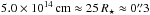 ). For the reason discussed in Sect. 4.4.1, we also considered an alternative H2O abundance profile with a sharp increase in H2O abundance near the radio photosphere.
In our radiative transfer modelling, the expansion/infall velocity, gas density, and gas kinetic temperature are the crucial parameters in the input physical model. We empirically explored different types of profiles that are plausible in the inner winds and circumstellar envelopes of evolved stars. To improve the readability of the article, we present in Appendix E various plausible models that fail to reproduce the observed spectra. In this section, we only discuss our preferred model − Model 3 − in which both infall and outflow layers coexist in the extended atmosphere of Mira. In Sect. 5.3, we compare the velocity, density, and temperature profiles in our preferred model with those predicted by current hydrodynamical models of pulsating stellar atmospheres. We also model the line radiative transfer with the atmospheric structures derived from those hydrodynamical models.
4.4.1. Preferred model: Mixed infall and outflow
Our modelling shows that pure infall would produce too much emission in the blueshifted velocities of the spectra than is observed (Appendix E). The excess emission component, as we have discussed in Sect. 3.3, originates from the far-side of the innermost layer (beyond the radio photosphere) of Mira’s extended atmosphere that is not blocked by the radio continuum disk. In our preferred model, we introduce a thin expanding layer (~5 × 1011 cm ≈ 0.03 R⋆) in the innermost radii between the radio photosphere and the globally infalling layer. Alternating outflow and infall velocity profiles have been calculated numerically by Bowen (1988a,b) for Mira-like variables, and subsequently adopted by Humphreys et al. (1996, 2001) to simulate the SiO and H2O masers from a Mira-like M-type variable star at a single stellar phase. The infall velocity immediately above this expanding layer is about 7.3 km s-1, and the expansion velocity below this layer is about 4.0 km s-1. The outer infalling gas and the inner expanding layer produce a shocked region with the shock velocity of ΔV ≲ 12 km s-1 near the radio photosphere of Mira. The maximum gas infall speed of ~7 km s-1 is consistent with the proper motions of SiO maser spots around another oxygen-rich Mira variable TX Cam, which lie in the velocity range of 5−10 km s-1 (Diamond & Kemball 2003). The emission from the far-side of the expanding layer would appear at redshifted velocities and the absorption from the near-side would be in the blueshifted part (i.e. the usual P Cygni profile). The excess emission from the pure infall models is therefore reduced to a level that fits the observed spectra.
To properly fit the line profiles, the radius of peak infall velocity adopted is 3.75 × 1013 cm, where the gas density is almost 1013 cm-3. Figure 9 shows the important input parameters in our model, including the molecular H2 gas density (top left), infall velocity (top right), molecular SiO and H2O abundances (middle), and the gas kinetic temperature (bottom). The bottom row of Fig. 9 also shows the excitation temperatures of the SiO and H2O transitions (in colour).
Figures 10−12 show the comparison of our modelled and observed spectra of SiO ν= 0J = 5−4, SiO ν= 2J = 5−4, and H2O v2 = 1JKa,Kc = 55,0−64,3, respectively. The top left panel of these figures show the spectra extracted from the line of sight towards the continuum centre.
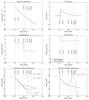 |
Fig. 9 Inputs of our preferred model. Shown in the panels are the H2 gas density (top left), infall velocity (negative represents expansion; top right), 28SiO abundance (middle left), H2O abundance (middle right), and the kinetic temperature (in black) and excitation temperatures (in colours) of the three 28SiO transitions (bottom left) and the H2O transition (bottom right). In the bottom right panel, the solid red line indicates positive excitation temperature (i.e. non-maser emission) of the H2O transition, and the dashed red line indicates the absolute values of the negative excitation temperature (i.e. population inversion) between 1.7 × 10¹⁴ and 2.4 × 1014 cm. Small negative values for the excitation temperature would give strong maser emission. Vertical dotted lines indicate the radii where the spectra were extracted; coloured horizontal dotted lines in the bottom panels indicates the upper-state energy (Eup/k) of the respective transitions. The innermost layer within Rcontinuum represents the grid cells for the pseudo-continuum, whose input values for H2 gas density and molecular abundances are above the range of the plots. |
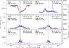 |
Fig. 10 Preferred model: spectra of SiO ν= 0J = 5−4 at various positions. The black histogram is the observed spectrum at the centre of continuum, green, blue, cyan, and magenta histograms are the observed spectra along the eastern, southern, western, and northern legs, respectively, at various offset radial distances as indicated in each panel. The red curves are the modelled spectra predicted by ratran. Our model does not produce the population inversion (i.e. negative excitation temperature) required for maser emission in this SiO transition, so we do not expect our modelled spectra to show any maser emission, as seen in the spike in the upper right panel (see text for the discussion of the spike). |
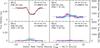 |
Fig. 11 Preferred model: spectra of SiO ν= 2J = 5−4 at various positions. The black histogram is the observed spectrum at the centre of continuum, green, blue, cyan, and magenta histograms are the observed spectra along the eastern, southern, western, and northern legs, respectively, at various offset radial distances as indicated in each panel. The red curves are the modelled spectra predicted by ratran. |
The top right panel of Fig. 10 shows the modelled and observed SiO spectra at 32 mas. In our modelled spectrum, there is a small absorption feature near the redshifted velocity of + 10 km s-1, which is not seen in the data. This spectral feature is indeed part of the broad absorption as seen along the line of sight towards the radio continuum, which appears in the spectra at 32 mas owing to beam convolution. Hence, we may have introduced too much absorption into the model, in particular near the peak infall velocities. Inhomogeneities in the images may have introduced additional emission features to the spectra, but this is not the case here. For example, there is a sharp spike in the observed spectra extracted from the southern position (in blue). This feature is due to an intensely emitting SiO clump at ~26 mas to the south of the continuum centre. The maximum brightness temperature of this clump in the map is ~2300 K. The intense emission from this clump is probably due to maser action; if it were thermal in nature, then one would also expect the corresponding 29SiO line to be detected with intense emission from this clump. However, this clump is too far away from the other positions from which the spectra were extracted to contribute significant emission. Another possible explanation is that the infall velocity in our model may decrease too quickly with radius. For example, at the offset of 64 mas, our modelled SiO ν= 0 spectrum appears to be narrower than the observed spectra (middle left panel of Fig. 10). We tried including a constant velocity layer of 1013 cm at the peak infall velocity, but we were not able to eliminate the absorption feature near + 10 km s-1. If we adopt a much higher temperature, up to about 2600 K, in the immediate proximity of the radio photosphere, then we would introduce too much blueshifted emission to the resultant spectra. Also, our spherically symmetric and homogeneous model obviously fails to reproduce the features arising in individual clumps.
In Fig. 12, we present two different models of the H2O spectral fitting using different input abundance profiles, which are plotted in the middle right panel of Fig. 9. As shown in the top left panel of Fig. 12, the modelled spectra using constant abundance profile (“Model 3 abundance”; in red) do not fit well to the observed H2O absorption spectra (in black) along the line of sight towards the continuum centre. In particular, the modelled spectrum does not show the strong observed absorption in the extreme redshifted velocities >10 km s-1. Hence, we have to introduce a sharp rise in the input H2O abundance by about 10 times, to 5.0 × 10⁻⁵, within the innermost region where the infall velocity peaks (“High H2O abundance”; in blue) in order to reproduce the strong redshifted absorption feature in the spectrum.
Overall, considering the complexity of Mira’s extended atmosphere and inner wind, we believe that Model 3 can satisfactorily reproduce most of the features in the observed SiO and H2O spectra in ALMA Band 6. We therefore adopt it as our preferred model and use it as the base model of our further tests in Sect. 5.
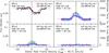 |
Fig. 12 Preferred model: spectra of H2O v2 = 1JKa,Kc = 55,0−64,3 at various positions. The black histogram is the observed spectrum at the centre of continuum, green, blue, cyan, and magenta histograms are the observed spectra along the eastern, southern, western, and northern legs, respectively, at various offset radial distances as indicated in each panel. The red curves are the modelled spectra predicted by ratran, and the blue dashed curves are the same model adopting a high H2O abundance (see the middle right panel of Fig. 9). |
5. Discussion
5.1. Caveat in the interpretation of the gas density
In our modelling, we assume that the gas in Mira’s extended atmosphere is composed of purely neutral, molecular hydrogen (H2) in its rotationally ground state, J = 0. At radii close to the radio photosphere of evolved stars, atomic hydrogen could be the dominant species in terms of number density (Glassgold & Huggins 1983; Doel 1990; Reid & Menten 1997a). Glassgold & Huggins (1983) have demonstrated that the atmosphere of an evolved star with the effective temperature of about 3000 K would be essentially atomic, and that the atmosphere of a star of about 2000 K would be essentially molecular. Since the effective temperature of the star is expected to be higher than the brightness temperature of the radio photosphere (e.g. Reid & Menten 1997a), there should be a significant amount of atomic hydrogen present in the regions being modelled. Intense hydrogen Balmer series emission lines have long been detected in the atmosphere of Mira (e.g. Joy 1926, 1947, 1954; Gillet et al. 1983; Fabas et al. 2011). The hydrogen emission is thought to be the result of dissociation and recombination of the atom due to shock waves propagating through the partially ionized hydrogen gas in the atmospheres of Mira variables (e.g. Fox et al. 1984; Fadeyev & Gillet 2004). In addition, molecular hydrogen could well be excited to higher rotational levels (see our discussion in Appendix D).
We note that the collisional rate coefficients between SiO molecule and atomic hydrogen (H) and electrons (e−) have already been computed by Palov et al. (2006) and Varambhia et al. (2009), respectively. However, in this study we did not attempt to calculate the fractional distribution of atomic/molecular hydrogen or to consider the collisions between SiO molecules and atomic hydrogen, helium, or electrons. Hence, the derived H2 gas density from our ratran modelling is just a proxy of the densities of all possible collisional partners of SiO, including rotationally excited molecular hydrogen, atomic hydrogen, helium, and even electrons, in the extended atmosphere of Mira.
In order to examine how well the H2 gas density in our preferred model is constrained, we modelled the SiO and H2O spectra by scaling the gas density by various factors. Figure 13 shows the results of these sensitivity tests on the input gas density. We find that the SiO spectra, extracted from the line of sight towards the centre of the continuum, does not vary too much, even if the gas density is varied by about an order of magnitude. On the other hand, the H2O spectra extracted from the centre shows significant change in the absorption depth even if the gas density is changed by a factor of ~2. Hence, assuming other input parameters (particularly the molecular abundances and gas temperature) of Model 3 are fixed, our derived gas density is tightly constrained. The gas density reaches 1012−1013 cm-3, just beyond the radio photosphere. This is consistent with other models that explain the radio continuum fluxes from Mira’s radio photosphere (Reid & Menten 1997a) and the near-infrared H2O spectrum (Yamamura et al. 1999). On the other hand, the derived gas density is much higher (by 2−4 orders of magnitude) than those predicted from hydrodynamical models (see Sect. 5.3.3).
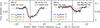 |
Fig. 13 Spectra of SiO ν= 0J = 5−4 (left) and H2O v2 = 1JKa,Kc = 55,0−64,3 (right) extracted from the centre of the continuum. The black histogram is the observed spectrum and the red curves are the modelled spectra from our preferred model, Model 3. The blue dashed curves are the spectra obtained by reducing the input H2 gas density by a factor of 5; and the green dotted curves are the spectra obtained by increasing the input gas density by a factor of 5 for the modelling of SiO, and a factor of 2 for H2O. |
5.2. Structure of the extended atmospheres
Our modelling results of the molecular emission and absorption of SiO and H2O gas allow us to compare the structure of the extended atmosphere of Mira as inferred from previous observations in various frequencies. We first briefly summarise the relevant observations of Mira in Sect. 5.2.1, then discuss our interpretation on Mira’s molecular layer in Sect. 5.2.2, and the dust condensation zone in Sect. 5.2.3.
5.2.1. Previous observations
Combining their centimetre-wavelength observations and millimetre/infrared fluxes in the literature, Reid & Menten (1997a) have demonstrated that long-period variables have a “radio photosphere” with a radius about twice that of the optical/infrared photosphere. The latter is determined from the line-free regions of the optical or infrared spectrum and is defined as the stellar radius, R⋆. In the following discussion, we adopt the value of R⋆ to be 12.3 mas (or 292 R⊙) as determined by Perrin et al. (2004). The spectral index in the radio wavelengths is found to be 1.86( ≈ 2), close to the Rayleigh-Jeans law at low frequencies of an optically thick blackbody (Reid & Menten 1997a). Matthews et al. (2015) and Planesas et al. (2016) found that this spectral index can also fit well the submillimetre flux densities of o Cet at 338 GHz in ALMA Band 7 and at 679 GHz in ALMA Band 9, respectively.
The radio photosphere encloses a hot, optically thick molecular layer (~2 × 10³ K) predominantly emitting in the infrared. Observations have revealed that this molecular layer lies between radii of ~1 and 2 R⋆. Haniff et al. (1995) found that, for o Cet, the derived radius of the strong TiO absorption near 710 nm with a uniform disk model is about 1.2 ± 0.2 R⋆. Perrin et al. (2004) have fitted a model consisting of an infrared photosphere and a thin, detached molecular (H2O+CO) layer to the infrared interferometric data, and have found that the radius of the molecular layer around o Cet is about 2.07 ± 0.02 R⋆. Alternatively, Yamamura et al. (1999) have modelled the H2O spectral features in the near-infrared (~2−5 μm) spectrum of o Cet with a stack of superposing plane-parallel layers: the star, an assumed hot SiO (2000 K) layer, a hot H2O (2000 K), and a cool H2O (1200 K) layers. Assuming the hot SiO layer has a radius of 2.0 R⋆, they have derived the radii of the hot and cool H2O layers to be 2.0 R⋆ and 2.3 R⋆, respectively. Ohnaka (2004) have employed a more realistic model for the extended molecular layer with two contiguous spherical shells, a hotter and a cooler H2O shell, above the mid-infrared photosphere. By fitting to the 11 μm spectrum, Ohnaka (2004) have derived the radii of 1.5 R⋆ and 2.2 R⋆ for the hot (1800 K) and cool (1400 K) H2O shells, respectively.
Beyond the molecular layer and the radio photosphere, there is a ring-like region of SiO maser emission at the radius between 2 R⋆ and 3 R⋆. Maser emission naturally arises from a ring-like structure because the maser requires a sufficiently long path length of similar radial velocity in order to be tangentially amplified to a detectable brightness (Diamond et al. 1994). Such a SiO maser ring has been imaged in detail at various stellar phases towards the oxygen-rich Mira variable TX Cam (e.g. Diamond & Kemball 2003; Yi et al. 2005). For o Cet, Reid & Menten (2007) have directly imaged the radio photosphere and the SiO J = 1−0 maser emission at 43 GHz and found that the radii of the radio photosphere and the SiO maser ring are about 2.1 R⋆ and 3.3 R⋆, respectively, with R⋆ = 12.29 ± 0.02 mas being the radius of the infrared photosphere as model-fitted by Perrin et al. (2004).
Further out, beyond the SiO maser emission region, dust grains start to form. The major types of dust around oxygen-rich AGB stars are corundum (Al2O3) and silicate dust. Using the hydrodynamical model from Ireland et al. (2004a,b), Gray et al. (2009) have modelled SiO maser emission in Mira variables and found that the presence of Al2O3 dust may either enhance or suppress SiO maser emission. From interferometric observations of various Mira variables at near-infrared (2.2 μm), mid-infrared (8−13 μm), and radio (43 GHz, 7 mm) wavelengths, Perrin et al. (2015) have fitted the visibility data with models similar to those of Perrin et al. (2004; stellar photosphere + detached shell of finite width) and found that Al2O3 dust predominantly forms between 3 R⋆ and 4.5 R⋆, while silicate dust forms in 12−16 R⋆, which is significantly beyond the radius of SiO maser emission and the silicate dust formation radius derived from previous observations (e.g. Danchi et al. 1994).
5.2.2. Molecular layer
From our visibility analysis (see Appendix A), we determine the mean radius of the 1.3 mm photosphere to be R229 GHz = 22.90 ± 0.05 mas (543 R⊙). This is about 1.9 times the size of the near-infrared photosphere (R⋆ = 12.3 mas; 292 R⊙) determined by Perrin et al. (2004). As we have summarised, previous visibility modelling of near- (2−5 μm) and mid-infrared (11 μm) interferometric data has suggested the existence of an optically thick, hot molecular H2O+SiO layer with a maximum radius of 2.3 R⋆ (~30 mas; Yamamura et al. 1999; Ohnaka 2004). Thus, this ALMA SV observation has a sufficient angular resolution to resolve the hot molecular layer in the millimetre-wavelength regime and, in addition, allows its velocity structure to be probed.
Modelling the spectral lines of H2O and SiO molecules at various projected radial distances from the star, we have determined that the kinetic gas temperature within the mid-infrared molecular layer (30 mas ~ 5 × 1013 cm) has to be about 1400−2100 K. The temperature range is consistent with those previously modelled by Reid & Menten (1997a) from their centimetre-wavelength observations of Mira’s radio photosphere, and by Yamamura et al. (1999) and Ohnaka (2004) from infrared observations using simple models of contiguous, uniform molecular H2O+SiO layers.
In our maps, the emission from the vibrationally excited (Eup/k> 3500 K) SiO ν= 2 and H2O v2 = 1 lines has an extent of ≲ 100 mas (≲ 8 R⋆). The core emission region of the SiO 5−4 ν= 0 vibrational ground state line (i.e. excluding the extended filamentary or arc-like emission feature to the west/south-west) that is detected at ≥3σ has radii between 200 mas (3.3 × 1014 cm; to the south-east) and 600 mas (9.9 × 1014 cm; to the west), and the size of the half-maximum emission is roughly 100−150 mas (see Fig. 2). Hence, SiO emits rotational emission up to a radius of ~50 R⋆, far beyond the radius of the molecular layer probed by infrared interferometers. Perrin et al. (2015), assuming that the mid-infrared N-band visibilities between 7.80 μm and 9.70 μm are the only signature of gas-phase SiO emission, concluded that the SiO can only be found in gas phase within 3 R⋆. We suggest that this discrepancy is due to the excitation effect of SiO molecules. The ground state SiO line in the ALMA SV observation has an energy above the ground of only ~30 K, and therefore is excited throughout the region within the silicate dust condensation zone. While the ALMA images indicate a significant amount of gas-phase SiO molecules, the gas temperature beyond the molecular layer (≲ 1000 K) is insufficient to collisionally excite the SiO molecules to higher vibrational states. Thus, the SiO molecule does not produce detectable infrared emission beyond ~3 R⋆ even if it is abundant there.
5.2.3. Dust shells and the sequence of dust condensation
The radii of dust shells around Mira were measured with infrared interferometry at 11 μm by Danchi et al. (1994) and Lopez et al. (1997). A single silicate dust shell from 60−2500 mas with a dust temperature of 1063 K at the inner radius was adopted in the model of Danchi et al. (1994). Lopez et al. (1997) used a two-shell model composed purely of silicate grains at radii of 50 mas and 200 mas. The dust temperature of the inner radius of the inner dust shell is about 1160−1380 K. These results suggest that dust grains start to form around Mira at a temperature above 1000 K and a radius of ~2−3 R⋆, where R⋆ was determined to be 19.3−23.6 mas. If we use our adopted value of 12.3 mas for R⋆, then the inner dust formation radius would be ~4−5 R⋆. Compared to the recent model of Perrin et al. (2015), this range is significantly smaller than the silicate formation radii, which is at least 12 R⋆, but is consistent with the radii of corundum formation.
Studies of silicate dust formation suggest that efficient condensation occurs only when the gas temperature drops to below 600 K (e.g. Gail & Sedlmayr 1998). This allows the SiO gas to emit to a much larger radius in the extended atmosphere of Mira than the radii of its dust shells derived previously and described above. The discussion of higher silicate dust condensation temperatures has been recently revived by Gail et al. (2013). Their new measurements of the vapour pressure of solid SiO suggest that gas-phase SiO molecules may first nucleate into SiO clusters and then condense onto dust grains (Gail et al. 2013). The gas temperature at which SiO gas start to deplete (also assumed to be the dust temperature at the inner boundary of the dust shell) is estimated to be about 600 K, for a mass-loss rate, Ṁ, of ~10-6M⊙ yr-1, increasing to 800 K for Ṁ = 10-4M⊙ yr-1. The SiO nucleation process thus allows the depletion of SiO gas to begin at a higher gas temperature, i.e. at a smaller inner radius, than previously thought. However, the result of Gail et al. (2013) still cannot explain the high dust temperature (>1000 K) as derived from visibility fitting by Danchi et al. (1994) and Lopez et al. (1997).
In our Model 3, the radius at which the 28SiO abundance decreases significantly is ~60 mas, which corresponds to 1.0 × 1014 cm or ~5 R⋆. The modelled gas temperature at this radius is ~600 K. In addition to this SiO abundance profile, we have also tested with other two-step functions in order to determine the maximum and minimum amount of SiO and the possible range of SiO depletion radii required to reproduce the observed ALMA spectra. Figure 14 shows three examples of alternative SiO abundance models. All these models are as good as our Model 3 in reproducing the spectra. Our experiments show that, at the very least, the SiO abundance should be ~1 × 10⁻⁶ within ~4 R⋆ and ~10-8−10-7 beyond that. In other words, SiO molecules cannot deplete onto dust grains in a significant amount within ~4 R⋆. This radius is consistent with the inner radius of the silicate dust shells derived in the literature. Our tests, however, have shown that the synthesised SiO spectra in the outer radii are not sensitive to a higher value of the SiO abundance, or the exact shape of the abundance profile. The actual radius where gas-phase SiO molecule condenses onto dust grains may therefore be much further from the star than 4 R⋆. Moreover, the actual degree of SiO gas depletion, through silicate dust condensation, nucleation of molecular clusters, or other gas-phase chemical reactions (e.g. Gail et al. 2013; Gobrecht et al. 2016), may not be as high as assumed in our preferred model.
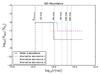 |
Fig. 14 Alternative input 28SiO abundance profiles for Model 3 which produce similar modelled spectra. The solid black curve is the same two-step abundance profile as in Model 3, which is close to the minimum possible abundance to fit the ALMA spectra. The three other coloured curves are alternative abundance profiles also using two-step functions. Abundance profile 1 (blue, dashed) has an inner abundance of 1 × 10⁻⁶ up to the radius of ~6 R⋆ and an outer abundance of 1 × 10⁻⁷; profile 2 (green, dash-dotted) has an inner abundance of 8 × 10⁻⁷ up to ~10 R⋆ and an outer abundance of 1 × 10⁻⁸; and profile 3 (red, dotted) has an inner abundance of 1 × 10⁻⁶ up to ~4 R⋆ and an outer abundance of 1 × 10⁻⁷. |
The gas temperature at which SiO gas starts to deplete in our models is about 490−600 K, far below the dust temperature at the inner dust shells as derived observationally by Danchi et al. (1994) and Lopez et al. (1997). This temperature is also somewhat lower, by about 100 K, than the gas temperature at which SiO gas starts to nucleate into clusters (Gail et al. 2013). However, we note that the visibility models derived by Danchi et al. (1994) and Lopez et al. (1997) have assumed that the dust around Mira is composed of pure silicate grains. The derived parameters are therefore based on the adopted optical properties of silicate dust grains. Other possible compositions of dust grains around oxygen-rich stars such as corundum or the mixture of corundum and silicate cannot be excluded, but have not been explored in those models.
Corundum, the crystalline form of aluminium oxide (Al2O3), has a high condensation temperature of ~1700 K (e.g. Grossman & Larimer 1974; Lorenz-Martins & Pompeia 2000) and is the most stable aluminium-containing species at a temperature below 1400 K (Gail & Sedlmayr 1998). Little-Marenin & Little (1990) classified the circumstellar dust shells of oxygen-rich AGB stars into several groups according to the spectral features found in their mid-infrared spectral energy distributions (SEDs). These SED groups show (a) broad emission features from 9 to 15 μm; (b) multiple components with peaks near 10, 11.3, and 13 μm; and (c) strong, well-defined characteristic silicate peaks at 9.8 and 18 μm. Little-Marenin & Little (1990) have also suggested that the circumstellar dust shells follow an evolutionary sequence starting from the class showing the broad feature, then multiple components, and finally silicate features in the SED. From a survey of O-rich AGB stars, most of which are Mira variables, Lorenz-Martins & Pompeia (2000) have successfully fitted the SEDs showing (a) broad features; (b) multiple components (or the intermediate class); and (c) silicate features and with corundum grains, a mixture of corundum and silicate grains, and pure silicate grains, respectively. Their results show that the inner radius of the modelled dust shells increases from the broad class, the intermediate class, and the silicate class. The fitted dust temperature of the hottest grains also follows the same sequence. In addition, they also found that the optical depths of the corundum-dominated emission are much smaller than those of the silicate-dominated emission. Lorenz-Martins & Pompeia (2000) thus concluded that their results were consistent with the evolutionary sequence suggested by Little-Marenin & Little (1990). Corundum grains are the first species to form in the circumstellar dust shells, at a small radius of ~2−3 R⋆ and a temperature of ~1400−1600 K. At a later stage, silicate grains start to form and dominate the emission features in the SED. The inner radius of the silicate dust shells and temperature of the hottest silicate grains are ~5−20 R⋆ and ~500−1000 K, respectively.
Our modelling results have shown that gas-phase SiO starts to deplete at a radius of at least 4 R⋆ and a gas temperature of ≲ 600 K. In addition, the observed spectra show that SiO molecules survive in the gas-phase well below 1000 K. This is apparently inconsistent with the fitting by Danchi et al. (1994) and Lopez et al. (1997) who found that the silicate dust shells form at a temperature above 1000 K. We therefore suggest that the inner hot dust shells around Mira may indeed be composed of other grain types, possibly corundum, instead of silicate grains as previously assumed. Although no prominent spectral features of corundum have been reported (e.g. Lopez et al. 1997; Lobel et al. 2000), we note that the corundum grains may be coated with silicates when the temperature becomes low further out in the dust shell (e.g. Karovicova et al. 2013, Sect. 6.1 and references therein). The optical depth of pure corundum grains, which only exist close to the star, may also be much lower than that of silicate grains (e.g. Lorenz-Martins & Pompeia 2000) and therefore the corundum features may not be easily distinguished in the SED from the silicate features.
5.2.4. Maser emission
Among all the spectral lines covered in this ALMA SV observation, only SiO ν= 1J = 5−4 and ν= 1J = 2−1 (in ALMA Band 3; not included in this article) exhibit strong maser emission (Fig. 8). In the images, isolated SiO ν= 1J = 5−4 maser spots are seen outside Mira’s radio photosphere, primarily at the radial distances between ~30 and 120 mas from the fitted position of the radio continuum. The relative spatial distribution of the SiO ν= 1 maser is consistent with those previously reported by Boboltz & Claussen (2004) and Cotton et al. (2008, and references therein) in other lower-J maser transitions. The presence of maser emission indicates that the SiO gas in those maser-emitting spots must not be in local thermodynamic equilibrium (LTE). In our preferred model (1D and smooth), the gas density is uniformly high throughout the maser-emitting region and hence all possible maser action is quenched. The predicted excitation temperature does not show any negative values throughout the modelled region (Fig. 9) and therefore population inversion, a prerequisite for maser emission to take place, of the SiO ν= 1 transition cannot be predicted by our simple model. We note that our model does not include any external infrared radiation field, in particular the infrared pumping band of SiO molecule near 8.1 μm (Δν = 1, fundamental) and 4.0 μm (Δν = 2, first overtone). The only input radiation field in our model is a blackbody of 2600 K representing the radio photosphere of Mira. This temperature is lower than the typical infrared effective temperature of Mira, which is about 3200 K (Woodruff et al. 2004). So the radiation field does not realistically approximate the radiative excitation of SiO molecule to higher vibrational states. Because our modelling aims to explain the general physical conditions of Mira’s extended atmosphere, we did not attempt to construct a sophisticated model to explain both maser and non-maser emission.
The water line covered in this SV observation, H2O v2 = 1 JKa,Kc = 55,0−64,3, near 232.7 GHz does not show any maser emission. Gray et al. (2016) have conducted extensive radiative transfer modelling to explore the physical conditions under which the modelled H2O lines (including all possible lines covered by ALMA) would exhibit maser emission in the envelopes of evolved stars. Slab geometry and silicate dust, which is optically thin in the millimetre wavelengths and optically thick in the radiative pumping bands of H2O’s vibrational states (e.g. the v2 band at 6.27 μm), have been assumed in their modelling (Gray et al. 2016). The 232.7 GHz H2O emission is seen from the radio photosphere up to about 80 mas (Fig. 6). Hence, the H2O-emitting region corresponds to the kinetic temperature of ~550−2100 K, the gas density of nH2 ~ 4 × 10¹⁰−1 × 1013 cm-3, and hence the H2O molecular density of nH2O ~ 2 × 10⁵−5 × 107 cm-3 in our preferred model. Our derived H2O molecular density lies well within the range in the model of Gray et al. (2016) that is predicted to exhibit strong maser emission in the 232.7 GHz transition if the dust temperature is high enough. The absence of the 232.7 GHz H2O maser is consistent with a silicate-type dust temperature lower than approximately 900, 1000, and 1600 K for the respective gas kinetic temperature of about 500, 1000, and 1500 K (see Fig. 10 of Gray et al. 2016). These comparisons, although not a conclusive proof, suggest that hot dust grains that are optically thick at the v2 band (6.27 μm) did not exist in Mira’s extended atmosphere during the ALMA SV observation.
5.3. Comparison with current hydrodynamic models
5.3.1. Early hydrodynamic models for stellar pulsation
There are many numerical hydrodynamical calculations on Mira variables to simulate the variation of pulsation velocity, number density, and kinetic temperature as functions of the stellar phase and/or radial distance from the star. Pioneering work includes the studies of Willson & Hill (1979), Hill & Willson (1979), Wood (1979), Willson (1987), as well as Beach et al. (1988) and Bowen (1988a,b, 1989), (hereafter Bowen’s models). Wood (1979), Willson (1987), and Bowen (1988a,b, 1989) have compared the effect of radiation pressure on dust on the mass-loss rate and the velocities of the stellar outflows. The outflow/infall velocity profiles as a function of radius as derived from these models are qualitatively similar. These authors all predict alternating outflow and infall layers in close proximity to the star, within about 4−6 × 1013 cm. Beyond that radius, the dust-driven winds exhibit accelerating outflow. In the region where material expands and falls back, large-scale shocks are produced at the interface between the outer infall layer and the inner outflow.
Infall motions in the extended atmosphere of the star can be observed as inverse P Cygni profiles in the spectra. The material at the near side of the star will show redshifted absorption and the material at the far side that is not blocked by the continuum will show blueshifted emission. These emission features are present even if there is no hot material (perhaps shock-heated) with a temperature higher than the continuum brightness temperature, and are also known as the “nebular” effect (e.g. Bessell et al. 1996; Scholz & Wood 2000), in which the large volume of the highly extended atmosphere, albeit only weakly emitting per unit volume, adds up to produce significant emission. For example, the redshifted absorption in the CO second overtone lines (Δν = 3) from o Cet indicates infall motions in the deep photospheric layers of the star (Hinkle et al. 1984). Results from the early spectroscopy by Joy (1926, 1954) also suggest infall motion in the extended atmosphere of o Cet based on modern information on the systemic (i.e. centre of mass) velocity of the star (see also the interpretation by Gabovitš 1936).
Bowen’s models were adopted by Humphreys et al. (1996) and Humphreys et al. (2001) to simulate the SiO (ν= 1 and 2) and H2O (ground state and v2 = 1) masers from a template M-type Mira (parameters were based on o Cet) at a single stellar phase, and by Gray & Humphreys (2000) and Humphreys et al. (2002) to simulate the variability of SiO (ν= 1) masers at various epochs of a stellar cycle of the model Mira. Gray et al. (2009) have comprehensively reviewed the success and limitations of these precursor models for SiO maser simulations. One major drawback of Bowen’s hydrodynamical solutions is that the pulsation phase in the model (with phase 0 defined as the moment when the inner boundary of the model atmosphere, or the “piston”, is moving outwards at the maximum speed) is disconnected from the stellar phase as determined from the optical or infrared brightness variations (Humphreys et al. 1996). In addition, the assumption of a constant infrared radiation field by dust and the stellar photosphere was also too simplistic for Mira variables (Gray et al. 2009).
Solving the hydrodynamical equations as presented in Richtmyer & Morton (1967, Chap. 12), who adopted the von Neumann-Richtmyer pseudo-viscosity method as the artificial shock dissipation mechanism (von Neumann & Richtmyer 1950), the authors of early hydrodynamic models derived the dynamical structures around Mira-like variables. Bowen’s models also considered the thermal relaxation of shocks via radiative cooling from neutral hydrogen atoms at high temperatures (≳ 6000 K) and from other species (which is represented by an assumed cooling coefficient) at low temperatures (see Sects. II(b) and II(c)(iii) of Bowen 1988a). Bowen’s models predicted the existence of an extended (~1014 cm) post-shock region of elevated gas temperatures (~10 000 K) near the optical/infrared photosphere.
On the other hand, using the hydrogen Balmer series emission lines as the signatures of shock-heated region, Fox et al. (1984) and Fox & Wood (1985) developed a theoretical model of shock waves in the atmosphere of Mira variables and predicted that these pulsation-driven shocks dissipate within a very thin region in the extended atmospheres, that is several orders of magnitude smaller than the stellar radius (i.e. ≪ 1012 cm). The circumstellar shock models by Willacy & Cherchneff (1998) and Gobrecht et al. (2016) predict that the cooling length of H2 dissociation, depending on the shock velocities, is typically < 108 cm. The very narrow post-shock region suggests that the relaxation of the shocked material towards radiative equilibrium and local thermodynamic equilibrium is essentially instantaneous and therefore the post-shock heating might be neglected. Woitke et al. (1996) argued that Bowen’s cooling rate was underestimated by a few orders of magnitude, thus resulting in an atmosphere with highly elevated gas temperature. Furthermore, based on the observational constraints from Mira’s radio continuum emission at 8 GHz, Reid & Menten (1997a,b) have shown that the amplitude of gas temperature disturbance, probably due to shocks or pulsations, can only be about 300 K (assuming a shock propagation speed of 7.3 km s-1). These are in contrast with Bowen’s non-equilibrium models which expect a rather extended shock-heated region with highly elevated gas temperature. Bessell et al. (1989) compared the synthesised spectra from Bowen’s non-equilibrium model with the observed spectrum between 600 nm and 4 μm, and found that they did not match at all. Moreover, the hydrogen spectra (e.g. Hα) predicted by Luttermoser & Bowen (1990, 1992) using Bowen’s model were much broader and had line profiles that were different to what was actually observed (Woodsworth 1995). Hence, the non-equilibrium models with extended high-temperature regions are not suitable for the extended atmospheres of Mira variables (see also the discussions in Woitke 1998; Willson 2000).
For the purpose of verification, we have also conducted similar tests to those of Bessell et al. (1989) by introducing into our preferred model (Model 3) an arbitrary extended layer (≳ 1012 cm) of elevated gas temperature (~4000 K) at various radial distances from Mira. The elevated temperature is significantly higher than the brightness temperature of the stellar radio continuum (~2600 K). Figure 15 shows an example of our tests. Even though the gas temperature is elevated for just a relatively thin layer (2 × 1013 cm ~ R⋆) compared to Bowen’s non-equilibrium model (~1014 cm), the synthesised spectra exhibit very strong emission features that are absent in the data. In fact, if we extend the zone of elevated gas temperature further, the emission spikes only become more prominent. Therefore our tests suggest that during this particular ALMA SV observation, the extended atmosphere of Mira did not contain an extended (≳ 1012 cm) shock-heated (above the brightness temperature of the radio continuum) region as was predicted from the non-equilibrium model. This is consistent with those shock wave models that suggest that the shock relaxation in the Mira atmosphere takes place within a very thin zone compared to the stellar radius (e.g. Fox et al. 1984; Fox & Wood 1985). In addition, we do not expect the existence of stellar chromosphere beyond the radio photosphere of Mira during this ALMA SV observation. Stellar chromosphere was suggested to explain the Hα absorption lines from some semi-regular variables (Luttermoser et al. 1994; Wood et al. 2004), but it may not exist around Mira at all because the Hα line from the star has only been seen in emission, not absorption (e.g. Joy 1947; Gillet et al. 1983, 1985).
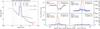 |
Fig. 15 Preferred model with a layer of an elevated gas temperature. The layer has a width of 2.0 × 1013 cm and an arbitrarily chosen temperature of 4000 K. The left panel shows the elevated gas temperature profiles and the right panel shows the observed and modelled SiO ν= 2J = 5−4 spectra as examples. All other parameters are the same as our preferred model (Model 3). |
5.3.2. More recent hydrodynamic models
Based on the assumption of negligible post-shock heating, Bessell et al. (1996) and Hofmann et al. (1998) made series of pulsation models to theoretically calculate the photospheric structure (e.g. density, temperature, outflow/infall velocities) of Mira variables. Applying the predictions from these model series, Bessell et al. (1996) and Scholz & Wood (2000) predicted the near-infrared spectra of selected atomic and molecular lines, which exhibit both the normal and inverse P Cygni profiles, and show significant variations with the stellar phase.
New hydrodynamical solutions have also been derived by Ireland et al. (2004a,b) and adopted by Gray et al. (2009) to simulate SiO maser emission in Mira variables. The model series are based on self-excited pulsation as in Hofmann et al. (1998), instead of piston-generated pulsation in other hydrodynamical models. Simulations have shown that SiO masers form a ring of typically ~2.2 R⋆ around the star (Gray et al. 2009), which is close to but beyond the radius of the radio photosphere. The results are consistent with the previous observations of SiO maser shells around Mira by Reid & Menten (1997a, 2007). Hence, strong SiO masers within the radio photosphere are prohibited (Reid & Menten 1997a; Gray et al. 2009). Comparing the hydrodynamical solutions of Ireland et al. (2004a,b) with observations, the strongest inner shocks (with ΔV> 20 km s-1) are enclosed within the radio photosphere, and the shocks beyond that only cause a velocity change of ~7 km s-1. The low shock velocity beyond the radio continuum is also consistent with the proper motion velocities of SiO masers observed in TX Cam (Diamond & Kemball 2003) and the nearly constant radio light curves observed in several Mira variables (Reid & Menten 1997a,b). In addition, Gray et al. (2009) have found that the presence of corundum (Al2O3) dust grains can both enhance or suppress SiO maser emission.
More recently, Ireland et al. (2008, 2011) and Scholz et al. (2014) have developed the Cool Opacity-sampling Dynamic EXtended (codex) atmosphere models, based on an improved self-excited pulsation code by Keller & Wood (2006) to determine the pressure and luminosity, and an opacity-sampling method to derive the gas and dust temperatures (see also the review by Ireland 2011). The mass density and velocity profiles in the extended atmosphere can also be computed. Thus far, the codex models have only been compared to the spectro-interferometric and spectro-photometric observations of Mira variables in the infrared wavelengths (e.g. Woodruff et al. 2009; Wittkowski et al. 2011; Hillen et al. 2012). Our radiative transfer modelling of the submillimetre molecular transitions from Mira as observed by the ALMA long baselines, including the vibrational ground state lines that are less affected by excitation effects, can provide an alternative probe to the detailed physical conditions in Mira’s extended atmosphere at a spatial scale of a few R⋆. In Sects. 5.3.3 and 5.3.4 we present our modelling results using the predicted atmospheric structures from codex and alternative velocity profiles in Mira’s extended atmosphere.
5.3.3. Kinematics
As described above, our high angular-resolution ALMA long baseline data clearly resolve the line emission/absorption from the extended atmosphere of Mira. Employing radiative transfer modelling we can test the atmospheric structures predicted by the latest hydrodynamical models. In particular, we consider the hydrodynamical model series, codex, developed by Ireland et al. (2008, 2011) and Scholz et al. (2014). We use the o54 5400 L⊙ model series, which is based on the stellar parameters of our target source, Mira (o Cet). From the codex developers we have obtained the atmospheric structure information of the o54 model series, including the total mass density, kinetic temperature (which is not the computed non-grey equilibrium temperature in the final model atmospheres; see Ireland et al. 2008), and the radial expansion or infall velocity of the gas at different radii. Among the six complete stellar pulsation cycles computed by the developers, the models at the stellar phases closest to this 2014 ALMA SV dataset (near phase 0.45) are models 25042015 (phase 0.38), 261740 (0.40), 286060 (0.41), 287880 (0.40), 289440 (0.40), and 291820 (0.41) (Ireland et al. 2008, 2011).
Because of the assumption of instantaneous shock dissipation, there is no extended zone of elevated gas kinetic temperature above the stellar brightness temperature in the extended atmosphere. The gas temperature profiles of the codex models are lower (by <500 K) and higher (by <700 K) than the values we empirically derive in Sect. 4.4 for the inner radii (≲ 5 × 1013 cm ≈ 2.5 R⋆) and outer radii, respectively. The temperature in Mira’s extended atmosphere is always <2000 K, except at radii very close to the radio continuum.
The codex code computes the mass density of all particles in the atmosphere. In our ratran input models, we convert the mass density to number density by division with the average mass of the particles in the wind, mpart = 0.7mH2 + 0.3mHe = 4.3372 × 10⁻²⁴ g, assuming the typical helium mass fraction of Y ≈ 0.3 (e.g. Wood & Cahn 1977; Lattanzio & Wood 2003; Ireland et al. 2008; Ventura et al. 2013). In our modelling, however, we only consider the collision of H2O and SiO with rotational ground-state H2 molecules.
However, if we apply this conversion to the input models, the number density in Mira’s extended atmosphere will be about 108−1010 cm-3, which is too low to excite the molecules and to produce significant emission or absorption in the synthesised spectra. The deep absorption features observed towards the continuum disk and the emission profiles towards various radial distances from the star can only be reproduced by arbitrarily increasing the converted number density by a large factor. In our modelling, therefore, we scale the number density of all codex models by a factor of 104 such that the density outside the radio photosphere reaches at least 1012 cm-3. This density is similar to the value adopted in our empirical modelling (Sect. 4), and is also consistent with that derived by Reid & Menten (1997a), who modelled the centimetre-wavelength radio fluxes from the radio photospheres of Mira variables (including Mira). Furthermore, the density is also compatible with the lower limit of 1011 cm-3, which is estimated by modelling the near-infrared H2O spectrum and assuming a relatively high H2O abundance of ~3 × 10⁻⁴ (Yamamura et al. 1999). If the adopted H2O abundance is similar to our assumed value of ~10-5, then the lower limit of the gas density derived by Yamamura et al. (1999) would also be close to the values in our modelling. We note, however, that the gas density should be interpreted with caution − see our discussion in Sect. 5.1.
In our initial test, we replaced our preferred model (Model 3) with the codex-predicted gas number density (scaled by 104), kinetic temperature, and radial velocity profiles. All other parameters, namely the SiO abundance profile, the local velocity dispersion, and the radio continuum, are the same as in Model 3. The outer radius of our model is greater than the outer boundaries of the codex models. The outer boundaries depend on individual codex models. For each model, we extrapolate the number density and kinetic temperature in power laws near the outer boundary, i.e. linear extrapolation in log-log relation. We also assume the infall or expansion velocity at and beyond the codex model boundary to be constant because we have no information of the kinematics beyond that. Since the gas density and molecular SiO abundance are usually too low to cause significant excitation in the outer regions, the precise extrapolation method has little effect on the synthesised spectra.
Figure 16 shows the results of our initial test of the velocity profiles from these six codex models. Remarkably, near the observed stellar phase all six models are able to qualitatively reproduce the general spectral features, including (1) the strong absorption profile in the line of sight towards the radio continuum of Mira and (2) gradually decreasing emission flux and line width in the lines of sight towards increasing radial offsets from the star. Closer inspection reveals that all six models produce an extra high-velocity absorption wing in either the redshifted or blueshifted part of the spectra towards the centre of the continuum. The velocities of the absorption wings correspond to the high-velocity gas at 10−20 km s-1 near the radio continuum of Mira, i.e. 3.6 × 1013 cm (1.8 R⋆). Because there is no sign of any absorption wings broader than ± 10 km s-1 in the observed spectra, the strong velocity variation as seen in these models, in particular models 261740, 286060, 287880, and 289440, cannot explain the specific atmosphere structure of Mira during the time of the 2014 ALMA SV observation.
The velocity profiles of codex models 250420 and 291820 are qualitatively similar to our Model 3 (see Fig. 9, top right panel). First, the extended atmosphere exhibits slowly varying, infall motion over a wide range of radii. Second, there is a sharp change in velocity, representing a strong shock front with ΔV ≳ 10 km s-1 just outside the radio continuum (3.60 × 1013 cm). The strong shock front in model 250420 is located at 3.64 × 1013 cm, and in model 291820 it is at 3.83 × 1013 cm (Ireland et al. 2011). In our second test, we increase the radius of our radio pseudo-continuum to engulf the strong shock fronts in models 250420 and 291820. Figure 17 shows the modelled spectra as a result of hiding the strong shock fronts. The high-velocity absorption wings in the blueshifted part of the SiO spectra extracted from the continuum centre has disappeared, and hence the synthesised spectra can now better fit the observed ALMA spectra. We therefore conclude that, at the time of the 2014 ALMA SV observation (stellar phase ~0.45), there is no strong shock with a high velocity of ΔV ≳ 20 km s-1 in the extended atmosphere of Mira beyond the radius of its 229-GHz radio photosphere. Furthermore, the infall and outflow velocities of the gas beyond the radio photosphere of Mira are bounded by ~7 km s-1 and ~4 km s-1, respectively.
Our finding is consistent with previous observations of SiO maser emission from other oxygen-rich Mira variables. For example, Wittkowski et al. (2007) found that the expansion velocity of the SiO maser-emitting shell around S Ori is about 10 km s-1 by fitting the projected radii of the maser spots and their line-of-sight velocities; Diamond & Kemball (2003) also found that the infall velocities of the SiO maser emission around TX Cam range from 5−10 km s-1 by tracing the proper motions of the maser spots. Based on their shock damping model, Reid & Menten (1997b) have excluded the shock propagation velocities significantly (by a few km s-1) higher than 7 km s-1 in order to explain the multi-epoch radio flux variation of Mira at 8 GHz, assuming that the amplitude of temperature disturbance due to shocks is ≳ 300 K or the factor of density compression is ≳ 2. Hence, any gas infall or outflow motion with speed above 10 km s-1 is unlikely beyond the radio photosphere of Mira, and therefore the very high-velocity shocks of ΔV ≳ 20 km s-1 as predicted by the codex models, in particular models 285180 (phase 0.80) and 287980 (phase 0.61) in the same o54 model series (Ireland et al. 2011), are not expected.
The above exercises have demonstrated that the atmospheric structures predicted by the codex models can qualitatively reproduce the general spectral features of the molecular transitions originating from the extended atmospheres and the inner wind of Mira. As already suggested by the authors of codex, the derived structures of the model atmosphere, such as the stellar radius, mass density, gas temperature, and velocity, exhibit significant cycle-to-cycle variations and appear to be chaotic (Ireland et al. 2011; Ireland 2011). The combination of the expansion/infall velocity profile and the locations of shock fronts are different in each cycle. It may take tens of stellar cycles (over a decade) for similar atmospheric structures to reappear (e.g. Fig. 1 of Ireland et al. 2011). We therefore expect that the radio and (sub)millimetre spectra of the molecular transitions would also exhibit significant cycle-to-cycle variation in addition to rapid variation within a single cycle. Long-term monitoring (multi-cycle and multi-epoch) of Mira variables with the ALMA long baseline is therefore necessary to fully test the predictions from hydrodynamical models, especially the amplitudes of pulsation-driven shocks above the radio photospheres of these stars.
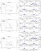 |
Fig. 16 Modified Model 3 with input gas density, kinetic temperature, and velocity profiles from codex models 250420 (top), 261740 (middle), and 286060 (bottom). Special scaling has been applied to the input gas density (see text). The infall velocity profiles are plotted on the left and the selected resultant spectra are shown on the right. We applied constant extrapolation of the infall velocity beyond the outer boundary of codex models. |
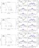 |
Fig. 16 Continued for codex models 287880 (top), 289440 (middle), and 291820 (bottom). |
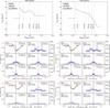 |
Fig. 17 Similar to Fig. 16, except that the radius of the pseudo-continuum in the model, Rcontinuum, is changed to 3.65 × 1013 cm for model 250420 (left column) and 3.85 × 1013 cm for model 291820 (right column). The modelled continuum levels are therefore slightly higher than those adopting Rcontinuum = 3.60 × 1013 cm. The strong shock fronts predicted in these two models are hidden inside the radio continuum. The middle and bottom rows show the selected resultant SiO spectra from the corresponding models. |
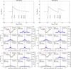 |
Fig. 18 Input radial velocity profile (top row) and modelled SiO (middle and bottom rows) spectra of two nearly identical models, except that for the model on the left there is only one large-scale velocity variation close to the radio continuum, while for the model on the right there is an additional strong velocity variation near 1.8 × 1014 cm = 109 mas ~ 5 R⋆. |
5.3.4. Wind acceleration
Höfner et al. (2003) also developed models of the dynamical atmospheres by solving time-dependent dynamic equations and frequency-dependent radiative transfer equations (i.e. non-grey dynamical model), including a time-dependent description of dust formation for carbon-rich atmospheres (see also the review by Höfner 2015). Based on Höfner’s hydrodynamical model, Gautschy-Loidl et al. (2004) were able to reproduce the infrared spectra of carbon-rich stars in the wavelength range of 0.5−25 μm, observed at various stellar phases, with a single consistent model atmosphere for each star. Nowotny et al. (2005a,b, 2010) have also compared the synthesised spectra of CO and CN in the infrared wavelengths with the observed spectra of carbon-rich stars and found that the general line profiles and radial velocities of the observed photospheric lines can be explained by the model atmospheres derived from the hydrodynamical code of Höfner et al. (2003). On the other hand, in the case of oxygen-rich model atmospheres, Höfner et al. (2003) have adopted a simple parametrised description for the dust opacity as in Eq. (5) of Bowen (1988a). If non-grey radiative transfer were considered in the dynamical models, however, there would be too little radiative pressure to drive the winds in oxygen-rich stars (e.g. Woitke 2006; Höfner & Andersen 2007). Both Woitke (2006) and Höfner (2007) have concluded that the iron content of the wind-driving dust grains must be low, otherwise the dust condensation radius would be too far away from the star (>10 R⋆) and hence dust-driven winds could not form. Höfner & Andersen (2007) have considered the possibility that the winds being driven by a small amount of carbon-bearing grains in the oxygen-rich atmospheres. By varying the grain properties in their dynamical models, Höfner (2008) has predicted that the size of the wind-driving (iron-free) grains must be in the narrow range between 0.1 and 10 μm. Scicluna et al. (2015) have reported the detection of large grains with an average size of ~0.5 μm in the oxygen-rich circumstellar envelope of the red supergiant (RSG) VY Canis Majoris based on optical polarimetric imaging. However, the implication of their results on AGB stars, which are the low-mass counterparts of RSGs, is unclear. In contrast, Ireland et al. (2011) and Ireland (2011) have found that both large iron-poor grains and small (<70 nm) iron-rich grains may drive the winds in oxygen-rich atmospheres, although the material still has to be lifted to a radius of at least 3−5 R⋆ where dust grains start to condense efficiently.
One notable difference between the results of the codex code and that developed by Höfner is that codex models exhibit large-scale velocity variations at radii up to ~10 R⋆, while the models based on Höfner’s code only show large-scale velocity variation of ΔV> 10 km s-1 within ~2−3 R⋆. In Höfner’s model atmospheres, the winds are efficiently accelerated by Fe-free dust grains that condense at ~3 R⋆ (e.g. Höfner 2009, 2015) and therefore the velocity profile becomes a generally continuous outflow with small-amplitude pulsation (ΔV ≲ 2 km s-1) due to previous shock episodes (e.g. Höfner et al. 2003; Nowotny et al. 2005a, 2010).
We have conducted another test to examine whether large-scale velocity variations of ΔV ~ 5 km s-1 at a large radial distance ~10 R⋆ from the star are possible. Instead of employing Höfner’s model atmospheres directly, we constructed a model nearly identical to our preferred Model 3 with a modified input velocity profile. Figure 18 shows the results of this test. The model in the left column presents the input velocity profile (top panel), the modelled and observed SiO ν= 0 (middle) and SiO ν= 2 (bottom) spectra of Model 3 for comparison. The model in the right column shows the input and results of the alternative velocity variation. This alternative model exhibits significant increase in the infall velocity, ΔV ≈ 6 km s-1 at ~9 R⋆, which can only be seen in Ireland’s codex atmospheres but not in Höfner’s. As long as the infall velocity does not exceed ~5 km s-1, the modelled spectra does not show a significant difference regardless of the radial distance where the gas from the extra shock episode is located. Based on the molecular spectra of Mira at this particular stellar phase alone, we cannot distinguish whether such an extra episode of shocked gas exists at all nor can we determine its possible distance from the star. On the other hand, our test concerning the SiO molecular abundance in Sect. 5.2.3 shows that the radius at which SiO starts to condense onto dust grains is at least 4 R⋆. This suggests that the actual wind acceleration may occur beyond ~4 R⋆ and hence some velocity variations could still be possible beyond ~2−3 R⋆.
6. Conclusions
-
1.
With the long ALMA baselines of~15 km, we are now able to probe the physical conditions in the extended atmospheres and the inner winds (within the dust condensation zone) of AGB stars in unprecedented detail. Mira (o Cet) has been observed as a Science Verification target in the 2014 ALMA Long Baseline Campaign. The angular resolution of the long baseline is ~30 mas at 220 GHz, which is high enough to resolve the radio continuum of Mira. For the first time, spectral line absorption against the stellar radio continuum has been clearly imaged in the millimetre wavelengths (1.3 mm) in the transitions of SiO ν= 0,1,2J = 5−4 and H2O v2 = 1JKa,Kc = 55,0−64,3.
-
2.
Through radiative transfer modelling, we are able to reconstruct the detailed physical conditions of Mira’s extended atmosphere, namely the gas density, kinetic temperature, abundance of SiO and H2O molecules, and the expansion/infall velocity as functions of radial distance from the star. We fit the SiO and H2O spectra along the lines of sight towards the stellar continuum and towards positions at various sky-projected radii and position angles from the star. In our preferred model, which successfully reproduces the spectra of SiO ν= 0,2 and H2O v2 = 1, the extended atmosphere shows infall motion in general. A shock of velocity ΔV ~ 12 km s-1 is found above Mira’s 229 GHz radio photosphere. The SiO abundance drops significantly from 1 × 10⁻⁶ to 1 × 10⁻⁸−1 × 10⁻⁷ at the radius of about 1.0 × 1014 cm = 5 R⋆, where R⋆ = 12.3 mas = 292 R⊙ is our adopted radius of Mira’s infrared photosphere. However, we have also shown that the SiO depletion radius may indeed be anywhere from 4 R⋆ outwards. In addition, the H2O spectra may be better fitted by adopting an abundance distribution that shows a sharp rise in abundance (of about 10 times) near the radio photosphere.
-
3.
We have also tested the predictions from current hydrodynamical models, in particular the codex model series that are tailored for Mira. We have used the predicted atmospheric structures as the inputs of our line radiative transfer modelling. The models are able to qualitatively reproduce the absorption features against the continuum. After fine-tuning the radial distances and the magnitudes of the major shock front(s), which are chaotic in nature, the synthesised spectra from the codex models can then fit the observed spectra in this SV observation reasonably well. Considering the chaotic nature of Mira’s extended atmosphere, the modelled spectra from the codex atmospheres fit the observed ALMA spectra remarkably well. In addition, we also demonstrated that some other models of Mira’s circumstellar environment (e.g. the presence of a chromosphere) do not have support in this ALMA data.
-
4.
We carried out model fitting of Mira’s radio continuum emission at 229.6 GHz and compared the results with two other independent results published in mid-2015. Our continuum models for Mira A and B are consistent with those fitted by Matthews et al. (2015). The single uniform disk model for Mira A is consistent with a radio photosphere with a brightness temperature of 2611 ± 51 K. On the other hand, we did not find any sign of a compact (~4.7 mas) hotspot (Tb ~ 10 000 K) in Mira A’s continuum as suggested by Vlemmings et al. (2015) even though we essentially adopted the identical fitting procedure and cross-checked with another visibility fitting software.
-
5.
The long ALMA baselines have demonstrated their capability to produce high-angular resolution and high-sensitivity spectral line images in the extended atmospheres of evolved stars. In order to test the validity of current hydrodynamical models and address the long-standing puzzle of dust condensation and wind-driving mechanism in oxygen-rich evolved stars, long-term monitoring (multi-cycle and multi-epoch) of Mira variables and AGB stars is necessary.
The period of Mira changes by a few days on a time span of decades (Templeton & Karovska 2009) and the dates of maximum need to be determined observationally for each cycle to provide a reliable phase scaling. In recent cycles, however, the phases preceding and during the maxima cannot be observed in the optical because Mira is too close to the Sun. To obtain the phases of the ALMA observations in 2014, we first phased the AAVSO data for the cycles in 2000−2013 with a period of 333 days and the date of maximum on JD 2 452 161.0, which had a bright and very well-defined maximum (Kamiński et al., in prep.). The data covering the cycle of the 2014 ALMA observations were then phased with the same period but their date of maximum (or phase 0) was determined by a phase shift of about + 0.05 with respect to JD 2 452 161.0 (as adopted for the 2000−2013 cycles). In this way we are able to match the data in the 2014 cycle with the phased data from 2000−2013 and therefore we obtain slightly later phases for the ALMA observations than those calculated from a periodicity scale given by AAVSO and used in Matthews et al. (2015).
Defined to be 0.6 × (wavelength/shortestbaseline) (Schieven 2015).
Available from the CASA Guides: http://casaguides.nrao.edu/index.php?title=ALMA2014_LBC_SVDATA&oldid=18077
These model numbers correspond to various phases of the models in the o54 series in chronological order. Models 248480−251160 are the models in the compact atmospheric cycles where most of the mass in the model atmosphere is contained within a relatively small radial extent, models 260820−263740 are those in the extended atmospheric cycles, and models 285180−291860 cover almost four consecutive pulsation cycles of the model atmosphere with intermediate extents of the mass-zones (see Fig. 1 and Tables 2−4 in Ireland et al. 2011).
NRAO Astronomical Image Processing System.
See footnote 2.
Acknowledgments
This paper makes use of the following ALMA data: ADS/JAO.ALMA#2011.0.00014.SV. ALMA is a partnership of ESO (representing its member states), NSF (USA) and NINS (Japan), together with NRC (Canada) and NSC and ASIAA (Taiwan), and KASI (Republic of Korea), in cooperation with the Republic of Chile. The Joint ALMA Observatory is operated by ESO, AUI/NRAO and NAOJ. We thank M. Scholz, M. J. Ireland, and P. R. Wood for kindly providing their model atmospheres from the o54 series of the Cool Opacity-sampling Dynamic EXtended (codex) atmosphere model. We thank M. J. Reid for a careful reading of the manuscript and for his highly useful comments. We also thank the anonymous referee and also L. D. Matthews and E. W. Greisen for their insightful comments and suggestions, which have inspired some of our tests to address the imaging issues. We acknowledge with thanks the variable star observations from the AAVSO International Database contributed by observers worldwide and used in this research. This research has made use of NASA’s Astrophysics Data System Bibliographic Services. This research has made use of the SIMBAD database, operated at CDS, Strasbourg, France. PyFITS is a product of the Space Telescope Science Institute, which is operated by AURA for NASA. K. T. Wong was supported for this research through a stipend from the International Max Planck Research School (IMPRS) for Astronomy and Astrophysics at the Universities of Bonn and Cologne and also by the Bonn-Cologne Graduate School of Physics and Astronomy (BCGS). K. T. Wong also acknowledges the BCGS Honors Budget which covers the digitisation cost of the Ph.D. thesis of R. C. Doel.
References
- Albrecht, M. A. 1983, A&A, 127, 409 [NASA ADS] [Google Scholar]
- ALMA Partnership, Fomalont, E. B., Vlahakis, C., et al. 2015, ApJ, 808, L1 [Google Scholar]
- Bajaja, E., & van Albada, G. D. 1979, A&A, 75, 251 [NASA ADS] [Google Scholar]
- Barber, R. J., Tennyson, J., Harris, G. J., & Tolchenov, R. N. 2006, MNRAS, 368, 1087 [NASA ADS] [CrossRef] [Google Scholar]
- Barton, E. J., Yurchenko, S. N., & Tennyson, J. 2013, MNRAS, 434, 1469 [NASA ADS] [CrossRef] [Google Scholar]
- Beach, T. E., Willson, L. A., & Bowen, G. H. 1988, ApJ, 329, 241 [NASA ADS] [CrossRef] [Google Scholar]
- Belov, S. P., Kozin, I. N., Polyansky, O. L., Tret’yakov, M. Y., & Zobov, N. F. 1987, J. Mol. Spectr., 126, 113 [NASA ADS] [CrossRef] [Google Scholar]
- Bessell, M. S., Brett, J. M., Wood, P. R., & Scholz, M. 1989, A&A, 213, 209 [NASA ADS] [Google Scholar]
- Bessell, M. S., Scholz, M., & Wood, P. R. 1996, A&A, 307, 481 [NASA ADS] [Google Scholar]
- Bieging, J. H., Knee, L. B. G., Latter, W. B., & Olofsson, H. 1998, A&A, 339, 811 [NASA ADS] [Google Scholar]
- Bieniek, R. J., & Green, S. 1981, Chem. Phys. Lett., 84, 380 [NASA ADS] [CrossRef] [Google Scholar]
- Bieniek, R. J., & Green, S. 1983a, ApJ, 265, L29 [NASA ADS] [CrossRef] [Google Scholar]
- Bieniek, R. J., & Green, S. 1983b, ApJ, 270, L101 [NASA ADS] [CrossRef] [Google Scholar]
- Boboltz, D. A., & Claussen, M. J. 2004, ApJ, 608, 480 [NASA ADS] [CrossRef] [Google Scholar]
- Bowen, G. H. 1988a, ApJ, 329, 299 [NASA ADS] [CrossRef] [Google Scholar]
- Bowen, G. H. 1988b, in Pulsation and Mass Loss in Stars, eds. R. Stalio, & L. A. Willson (Dordrecht: Kluwer Academic Publishers), Astrophys. Space Sci. Lib., 148, 3 [Google Scholar]
- Bowen, G. H. 1989, in Evolution of Peculiar Red Giant Stars, eds. H. R. Johnson, & B. Zuckerman (Cambridge: Cambridge University Press), IAU Colloq., 106, 269 [Google Scholar]
- Braun, R., & Walterbos, R. A. M. 1985, A&A, 143, 307 [NASA ADS] [Google Scholar]
- Carrillo, R. E., McEwen, J. D., & Wiaux, Y. 2014, MNRAS, 439, 3591 [NASA ADS] [CrossRef] [MathSciNet] [Google Scholar]
- Clark, B. G. 1980, A&A, 89, 377 [NASA ADS] [Google Scholar]
- Cornwell, T. J., Uson, J. M., & Haddad, N. 1992, A&A, 258, 583 [NASA ADS] [Google Scholar]
- Cotton, W. D., Mennesson, B., Diamond, P. J., et al. 2004, A&A, 414, 275 [NASA ADS] [CrossRef] [EDP Sciences] [Google Scholar]
- Cotton, W. D., Perrin, G., & Lopez, B. 2008, A&A, 477, 853 [NASA ADS] [CrossRef] [EDP Sciences] [Google Scholar]
- Dabrowski, I. 1984, Can. J. Phys., 62, 1639 [NASA ADS] [CrossRef] [Google Scholar]
- Danchi, W. C., Bester, M., Degiacomi, C. G., Greenhill, L. J., & Townes, C. H. 1994, AJ, 107, 1469 [NASA ADS] [CrossRef] [Google Scholar]
- Daniel, F., Dubernet, M.-L., & Grosjean, A. 2011, A&A, 536, A76 [NASA ADS] [CrossRef] [EDP Sciences] [Google Scholar]
- Dayou, F., & Balança, C. 2006, A&A, 459, 297 [NASA ADS] [CrossRef] [EDP Sciences] [Google Scholar]
- de Jong, T., Dalgarno, A., & Chu, S.-I. 1975, ApJ, 199, 69 [NASA ADS] [CrossRef] [Google Scholar]
- Decin, L., De Beck, E., Brünken, S., et al. 2010, A&A, 516, A69 [NASA ADS] [CrossRef] [EDP Sciences] [Google Scholar]
- DePristo, A. E., Augustin, S. D., Ramaswamy, R., & Rabitz, H. 1979, J. Chem. Phys., 71, 850 [NASA ADS] [CrossRef] [Google Scholar]
- Desmurs, J.-F., Bujarrabal, V., Lindqvist, M., et al. 2014, A&A, 565, A127 [NASA ADS] [CrossRef] [EDP Sciences] [Google Scholar]
- Diamond, P. J., & Kemball, A. J. 2003, ApJ, 599, 1372 [NASA ADS] [CrossRef] [Google Scholar]
- Diamond, P. J., Kemball, A. J., Junor, W., et al. 1994, ApJ, 430, L61 [NASA ADS] [CrossRef] [Google Scholar]
- Doel, R. C. 1990, Ph.D. Thesis, University of Bristol, available from http://ethos.bl.uk/OrderDetails.do?uin=uk.bl.ethos.667872 [Google Scholar]
- Doel, R. C., Gray, M. D., Humphreys, E. M. L., Braithwaite, M. F., & Field, D. 1995, A&A, 302, 797 [NASA ADS] [Google Scholar]
- Edmonds, A. R. 1960, Angular Momentum in Quantum Mechanics, the second edn. (3rd printing) (Princeton: Princeton University Press) [Google Scholar]
- Fabas, N., Lèbre, A., & Gillet, D. 2011, A&A, 535, A12 [NASA ADS] [CrossRef] [EDP Sciences] [Google Scholar]
- Fadeyev, Y. A., & Gillet, D. 2004, A&A, 420, 423 [NASA ADS] [CrossRef] [EDP Sciences] [Google Scholar]
- Faure, A., & Josselin, E. 2008, A&A, 492, 257 [NASA ADS] [CrossRef] [EDP Sciences] [Google Scholar]
- Feast, M. W., Glass, I. S., Whitelock, P. A., & Catchpole, R. M. 1989, MNRAS, 241, 375 [NASA ADS] [CrossRef] [Google Scholar]
- Field, D. 1998, in The Molecular Astrophysics of Stars and Galaxies, eds. T. W. Hartquist, & D. A. Williams (Oxford: Clarendon Press), International Series in Astronomy and Astrophysics, 4, 313 [Google Scholar]
- Flower, D. R. 1989, Phys. Rep., 174, 1 [Google Scholar]
- Fox, M. W., & Wood, P. R. 1985, ApJ, 297, 455 [NASA ADS] [CrossRef] [Google Scholar]
- Fox, M. W., Wood, P. R., & Dopita, M. A. 1984, ApJ, 286, 337 [NASA ADS] [CrossRef] [Google Scholar]
- Gabovitš, J. 1936, Publications of the Tartu Astronomical Observatory, 29, 1 [Google Scholar]
- Gail, H.-P., & Sedlmayr, E. 1998, Faraday Discussions, 109, 303 [Google Scholar]
- Gail, H.-P., Wetzel, S., Pucci, A., & Tamanai, A. 2013, A&A, 555, A119 [NASA ADS] [CrossRef] [EDP Sciences] [Google Scholar]
- Gautschy-Loidl, R., Höfner, S., Jørgensen, U. G., & Hron, J. 2004, A&A, 422, 289 [NASA ADS] [CrossRef] [EDP Sciences] [Google Scholar]
- Gillet, D., Maurice, E., & Baade, D. 1983, A&A, 128, 384 [NASA ADS] [Google Scholar]
- Gillet, D., Ferlet, R., Maurice, E., & Bouchet, P. 1985, A&A, 150, 89 [NASA ADS] [Google Scholar]
- Glassgold, A. E., & Huggins, P. J. 1983, MNRAS, 203, 517 [NASA ADS] [Google Scholar]
- Gobrecht, D., Cherchneff, I., Sarangi, A., Plane, J. M. C., & Bromley, S. T. 2016, A&A, 585, A6 [NASA ADS] [CrossRef] [EDP Sciences] [Google Scholar]
- Goldflam, R., Kouri, D. J., & Green, S. 1977, J. Chem. Phys., 67, 4149 [NASA ADS] [CrossRef] [Google Scholar]
- Gordon, R. G., & Kim, Y. S. 1972, J. Chem. Phys., 56, 3122 [NASA ADS] [CrossRef] [Google Scholar]
- Gray, M. D., & Humphreys, E. M. L. 2000, New Astron., 5, 155 [NASA ADS] [CrossRef] [Google Scholar]
- Gray, M. D., Wittkowski, M., Scholz, M., et al. 2009, MNRAS, 394, 51 [NASA ADS] [CrossRef] [Google Scholar]
- Gray, M. D., Baudry, A., Richards, A. M. S., et al. 2016, MNRAS, 456, 374 [NASA ADS] [CrossRef] [Google Scholar]
- Grossman, L., & Larimer, J. W. 1974, Rev. Geophys. Space Phys., 12, 71 [NASA ADS] [CrossRef] [MathSciNet] [Google Scholar]
- Haniff, C. A., Scholz, M., & Tuthill, P. G. 1995, MNRAS, 276, 640 [NASA ADS] [CrossRef] [Google Scholar]
- Hill, S. J., & Willson, L. A. 1979, ApJ, 229, 1029 [NASA ADS] [CrossRef] [Google Scholar]
- Hillen, M., Verhoelst, T., Degroote, P., Acke, B., & van Winckel, H. 2012, A&A, 538, L6 [NASA ADS] [CrossRef] [EDP Sciences] [Google Scholar]
- Hinkle, K. H., Hall, D. N. B., & Ridgway, S. T. 1982, ApJ, 252, 697 [NASA ADS] [CrossRef] [Google Scholar]
- Hinkle, K. H., Scharlach, W. W. G., & Hall, D. N. B. 1984, ApJS, 56, 1 [NASA ADS] [CrossRef] [Google Scholar]
- Hofmann, K.-H., Scholz, M., & Wood, P. R. 1998, A&A, 339, 846 [NASA ADS] [Google Scholar]
- Höfner, S. 2007, in Why Galaxies Care About AGB Stars: Their Importance as Actors and Probes, eds. F. Kerschbaum, C. Charbonnel, & R. F. Wing, ASP Conf. Ser., 378, 145 [Google Scholar]
- Höfner, S. 2008, A&A, 491, L1 [NASA ADS] [CrossRef] [EDP Sciences] [Google Scholar]
- Höfner, S. 2009, in Cosmic Dust − Near and Far, eds. T. Henning, E. Grün, & J. Steinacker, ASP Conf. Ser., 414, 3 [Google Scholar]
- Höfner, S. 2015, in Why Galaxies Care about AGB Stars III: A Closer Look in Space and Time, eds. F. Kerschbaum, R. F. Wing, & J. Hron, ASP Conf. Ser., 497, 333 [Google Scholar]
- Höfner, S., & Andersen, A. C. 2007, A&A, 465, L39 [NASA ADS] [CrossRef] [EDP Sciences] [Google Scholar]
- Höfner, S., Gautschy-Loidl, R., Aringer, B., & Jørgensen, U. G. 2003, A&A, 399, 589 [NASA ADS] [CrossRef] [EDP Sciences] [Google Scholar]
- Högbom, J. A. 1974, A&AS, 15, 417 [NASA ADS] [Google Scholar]
- Hogerheijde, M. R., & van der Tak, F. F. S. 2000, A&A, 362, 697 [NASA ADS] [Google Scholar]
- Humphreys, E. M. L., Gray, M. D., Yates, J. A., et al. 1996, MNRAS, 282, 1359 [NASA ADS] [CrossRef] [Google Scholar]
- Humphreys, E. M. L., Yates, J. A., Gray, M. D., Field, D., & Bowen, G. H. 2001, A&A, 379, 501 [NASA ADS] [CrossRef] [EDP Sciences] [Google Scholar]
- Humphreys, E. M. L., Gray, M. D., Yates, J. A., et al. 2002, A&A, 386, 256 [NASA ADS] [CrossRef] [EDP Sciences] [Google Scholar]
- Hunter, J. D. 2007, Comput. Sci. Engrg., 9, 90 [Google Scholar]
- Ireland, M. J. 2011, in Why Galaxies Care about AGB Stars II: Shining Examples and Common Inhabitants, eds. F. Kerschbaum, T. Lebzelter, & R. F. Wing, ASP Conf. Ser., 445, 83 [Google Scholar]
- Ireland, M. J., Scholz, M., Tuthill, P. G., & Wood, P. R. 2004a, MNRAS, 355, 444 [NASA ADS] [CrossRef] [Google Scholar]
- Ireland, M. J., Scholz, M., & Wood, P. R. 2004b, MNRAS, 352, 318 [NASA ADS] [CrossRef] [Google Scholar]
- Ireland, M. J., Scholz, M., & Wood, P. R. 2008, MNRAS, 391, 1994 [NASA ADS] [CrossRef] [Google Scholar]
- Ireland, M. J., Scholz, M., & Wood, P. R. 2011, MNRAS, 418, 114 [NASA ADS] [CrossRef] [Google Scholar]
- Jones, E., Oliphant, E., Peterson, P., et al. 2001, SciPy: Open source scientific tools for Python, http://www.scipy.org/ [Google Scholar]
- Joy, A. H. 1926, ApJ, 63, 281 [NASA ADS] [CrossRef] [Google Scholar]
- Joy, A. H. 1947, ApJ, 106, 288 [NASA ADS] [CrossRef] [Google Scholar]
- Joy, A. H. 1954, ApJS, 1, 39 [NASA ADS] [CrossRef] [Google Scholar]
- Junklewitz, H., Bell, M. R., Selig, M., & Enßlin, T. A. 2016, A&A, 586, A76 [NASA ADS] [CrossRef] [EDP Sciences] [Google Scholar]
- Karovicova, I., Wittkowski, M., Boboltz, D. A., et al. 2011, A&A, 532, A134 [NASA ADS] [CrossRef] [EDP Sciences] [Google Scholar]
- Karovicova, I., Wittkowski, M., Ohnaka, K., et al. 2013, A&A, 560, A75 [NASA ADS] [CrossRef] [EDP Sciences] [Google Scholar]
- Keller, S. C., & Wood, P. R. 2006, ApJ, 642, 834 [NASA ADS] [CrossRef] [Google Scholar]
- Kholopov, P. N. 1987, General Catalogue of Variable Stars, the fourth edn. (Moscow: Publishing House of the Academy of Sciences of the U.S.S.R.) [Google Scholar]
- Kłos, J., & Lique, F. 2008, MNRAS, 390, 239 [NASA ADS] [CrossRef] [Google Scholar]
- Langer, S. H., & Watson, W. D. 1984, ApJ, 284, 751 [NASA ADS] [CrossRef] [Google Scholar]
- Lattanzio, J. C., & Wood, P. R. 2003, in Asymptotic giant branch stars, eds. H. J. Habing, & H. Olofsson (New York: Springer Science+Business Media), Astron. Astrophys. Lib., 23 [Google Scholar]
- Lebzelter, T., Hinkle, K. H., Wood, P. R., Joyce, R. R., & Fekel, F. C. 2005, A&A, 431, 623 [NASA ADS] [CrossRef] [EDP Sciences] [Google Scholar]
- Lewars, E. G. 2011, Computational Chemistry: Introduction to the Theory and Applications of Molecular and Quantum Mechanics, the 2nd edn. (Dordrecht: Springer Science+Business Media B.V.) [Google Scholar]
- Lique, F., & Kłos, J. 2008, J. Chem. Phys., 128, 034306 [NASA ADS] [CrossRef] [Google Scholar]
- Little-Marenin, I. R., & Little, S. J. 1990, AJ, 99, 1173 [NASA ADS] [CrossRef] [Google Scholar]
- Lobel, A., Bagnulo, S., Doyle, J. G., & Power, C. 2000, MNRAS, 317, 391 [NASA ADS] [CrossRef] [Google Scholar]
- Lochner, M., Natarajan, I., Zwart, J. T. L., et al. 2015, MNRAS, 450, 1308 [NASA ADS] [CrossRef] [Google Scholar]
- Lockett, P., & Elitzur, M. 1992, ApJ, 399, 704 [NASA ADS] [CrossRef] [Google Scholar]
- Lopez, B., Danchi, W. C., Bester, M., et al. 1997, ApJ, 488, 807 [NASA ADS] [CrossRef] [Google Scholar]
- Lorenz-Martins, S., & Pompeia, L. 2000, MNRAS, 315, 856 [NASA ADS] [CrossRef] [Google Scholar]
- Luttermoser, D. G., & Bowen, G. H. 1990, in Cool Stars, Stellar Systems, and the Sun, ed. G. Wallerstein,ASP Conf. Ser., 9, 491 [Google Scholar]
- Luttermoser, D. G., & Bowen, G. H. 1992, in Cool Stars, Stellar Systems, and the Sun, eds. M. S. Giampapa, & J. A. Bookbinder,ASP Conf. Ser., 26, 558 [Google Scholar]
- Luttermoser, D. G., Johnson, H. R., & Eaton, J. 1994, ApJ, 422, 351 [NASA ADS] [CrossRef] [Google Scholar]
- Martí-Vidal, I., Vlemmings, W. H. T., Muller, S., & Casey, S. 2014, A&A, 563, A136 [NASA ADS] [CrossRef] [EDP Sciences] [Google Scholar]
- Matthews, L. D., Reid, M. J., & Menten, K. M. 2015, ApJ, 808, 36 [NASA ADS] [CrossRef] [Google Scholar]
- McMullin, J. P., Waters, B., Schiebel, D., Young, W., & Golap, K. 2007, in Astronomical Data Analysis Software and Systems XVI, eds. R. A. Shaw, F. Hill, & D. J. Bell, ASP Conf. Ser., 376, 127 [Google Scholar]
- Messiah, A. 1962, Quantum mechanics, Vol. II, the first edn. (4th printing) (Amsterdam: North-Holland Publication) [Google Scholar]
- Müller, H. S. P., Thorwirth, S., Roth, D. A., & Winnewisser, G. 2001, A&A, 370, L49 [NASA ADS] [CrossRef] [EDP Sciences] [Google Scholar]
- Müller, H. S. P., Schlöder, F., Stutzki, J., & Winnewisser, G. 2005, J. Molec. Struct., 742, 215 [CrossRef] [Google Scholar]
- Müller, H. S. P., Spezzano, S., Bizzocchi, L., et al. 2013, J. Phys. Chem. A, 117, 13843 [CrossRef] [Google Scholar]
- Nowotny, W., Aringer, B., Höfner, S., Gautschy-Loidl, R., & Windsteig, W. 2005a, A&A, 437, 273 [NASA ADS] [CrossRef] [EDP Sciences] [Google Scholar]
- Nowotny, W., Lebzelter, T., Hron, J., & Höfner, S. 2005b, A&A, 437, 285 [NASA ADS] [CrossRef] [EDP Sciences] [Google Scholar]
- Nowotny, W., Höfner, S., & Aringer, B. 2010, A&A, 514, A35 [NASA ADS] [CrossRef] [EDP Sciences] [Google Scholar]
- Ohnaka, K. 2004, A&A, 424, 1011 [NASA ADS] [CrossRef] [EDP Sciences] [Google Scholar]
- Ohnaka, K. 2014, A&A, 561, A47 [NASA ADS] [CrossRef] [EDP Sciences] [Google Scholar]
- Ohnaka, K., Bergeat, J., Driebe, T., et al. 2005, A&A, 429, 1057 [NASA ADS] [CrossRef] [EDP Sciences] [Google Scholar]
- Palov, A. P., Gray, M. D., Field, D., & Balint-Kurti, G. G. 2006, ApJ, 639, 204 [NASA ADS] [CrossRef] [Google Scholar]
- Perrin, G., Ridgway, S. T., Mennesson, B., et al. 2004, A&A, 426, 279 [NASA ADS] [CrossRef] [EDP Sciences] [Google Scholar]
- Perrin, G., Cotton, W. D., Millan-Gabet, R., & Mennesson, B. 2015, A&A, 576, A70 [NASA ADS] [CrossRef] [EDP Sciences] [Google Scholar]
- Planesas, P., Alcolea, J., & Bachiller, R. 2016, A&A, 586, A69 [NASA ADS] [CrossRef] [EDP Sciences] [Google Scholar]
- Ramaswamy, R., Depristo, A. E., & Rabitz, H. 1979, Chem. Phys. Lett., 61, 495 [NASA ADS] [CrossRef] [Google Scholar]
- Ramstedt, S., Mohamed, S., Vlemmings, W. H. T., et al. 2014, A&A, 570, L14 [NASA ADS] [CrossRef] [EDP Sciences] [Google Scholar]
- Reid, M. J., & Goldston, J. E. 2002, ApJ, 568, 931 [NASA ADS] [CrossRef] [Google Scholar]
- Reid, M. J., & Menten, K. M. 1997a, ApJ, 476, 327 [NASA ADS] [CrossRef] [Google Scholar]
- Reid, M. J., & Menten, K. M. 1997b, Ap&SS, 251, 41 [NASA ADS] [CrossRef] [Google Scholar]
- Reid, M. J., & Menten, K. M. 2007, ApJ, 671, 2068 [NASA ADS] [CrossRef] [Google Scholar]
- Richtmyer, R. D., & Morton, K. W. 1967, Difference Methods for Initial-Value Problems, the second edn. (New York: John Wiley & Sons) [Google Scholar]
- Robertson, B. S. C., & Feast, M. W. 1981, MNRAS, 196, 111 [NASA ADS] [CrossRef] [Google Scholar]
- Rupen, M. P. 1999, in Synthesis Imaging in Radio Astronomy II, eds. G. B. Taylor, C. L. Carilli, & R. A. Perley, ASP Conf. Ser., 180, 229 [Google Scholar]
- Sault, R. J. 1994, A&AS, 107, 55 [NASA ADS] [Google Scholar]
- Sault, R. J., Teuben, P. J., & Wright, M. C. H. 1995, in Astronomical Data Analysis Software and Systems IV, eds. R. A. Shaw, H. E. Payne, & J. J. E. Hayes, ASP Conf. Ser., 77, 433 [Google Scholar]
- Schieven, G. 2015, Observing with ALMA: A Primer for Early Science, ALMA Doc. 3.1, ver. 4 [Google Scholar]
- Schöier, F. L., van der Tak, F. F. S., van Dishoeck, E. F., & Black, J. H. 2005, A&A, 432, 369 [NASA ADS] [CrossRef] [EDP Sciences] [Google Scholar]
- Scholz, M., & Wood, P. R. 2000, A&A, 362, 1065 [NASA ADS] [Google Scholar]
- Scholz, M., Ireland, M. J., & Wood, P. R. 2014, A&A, 565, A119 [NASA ADS] [CrossRef] [EDP Sciences] [Google Scholar]
- Scicluna, P., Siebenmorgen, R., Wesson, R., et al. 2015, A&A, 584, L10 [NASA ADS] [CrossRef] [EDP Sciences] [Google Scholar]
- Sokoloski, J. L., & Bildsten, L. 2010, ApJ, 723, 1188 [NASA ADS] [CrossRef] [Google Scholar]
- Sutter, P. M., Wandelt, B. D., McEwen, J. D., et al. 2014, MNRAS, 438, 768 [NASA ADS] [CrossRef] [Google Scholar]
- Templeton, M. R., & Karovska, M. 2009, ApJ, 691, 1470 [NASA ADS] [CrossRef] [Google Scholar]
- Tennyson, J., Zobov, N. F., Williamson, R., Polyansky, O. L., & Bernath, P. F. 2001, J. Phys. Chem. Ref. Data, 30, 735 [NASA ADS] [CrossRef] [Google Scholar]
- Terlouw, J. P., & Vogelaar, M. G. R. 2015, Kapteyn Package, version 2.3, Kapteyn Astronomical Institute, Groningen, available from http://www.astro.rug.nl/software/kapteyn/ [Google Scholar]
- Thomas, L. D., Kraemer, W. P., & Diercksen, G. H. F. 1980, Chem. Phys., 51, 131 [NASA ADS] [CrossRef] [Google Scholar]
- Thompson, A. R., Moran, J. M., & Swenson, Jr., G. W. 2001, Interferometry and Synthesis in Radio Astronomy, the 2nd edn. (Weinheim: WILEY-VCH Verlag GmbH & Co. KGaA) [Google Scholar]
- Tsuji, T. 2000, ApJ, 540, L99 [NASA ADS] [CrossRef] [Google Scholar]
- Tsuji, T., Ohnaka, K., Hinkle, K. H., & Ridgway, S. T. 1994, A&A, 289, 469 [NASA ADS] [Google Scholar]
- Tsuji, T., Ohnaka, K., Aoki, W., & Yamamura, I. 1997, A&A, 320, L1 [NASA ADS] [Google Scholar]
- Turner, B. E., Chan, K.-W., Green, S., & Lubowich, D. A. 1992, ApJ, 399, 114 [NASA ADS] [CrossRef] [Google Scholar]
- van der Walt, S., Colbert, S. C., & Varoquaux, G. 2011, Comput. Sci. Engng., 13, 22, http://www.numpy.org/ [Google Scholar]
- van Langevelde, H. J., & Cotton, W. D. 1990, A&A, 239, L5 [NASA ADS] [Google Scholar]
- van Leeuwen, F. 2007, A&A, 474, 653 [NASA ADS] [CrossRef] [EDP Sciences] [Google Scholar]
- Varambhia, H. N., Gupta, M., Faure, A., Baluja, K. L., & Tennyson, J. 2009, J. Phys. B At. Mol. Phys., 42, 095204 [NASA ADS] [CrossRef] [Google Scholar]
- Ventura, P., Di Criscienzo, M., Carini, R., & D’Antona, F. 2013, MNRAS, 431, 3642 [NASA ADS] [CrossRef] [Google Scholar]
- Vlemmings, W. H. T., Ramstedt, S., O’Gorman, E., et al. 2015, A&A, 577, L4 [NASA ADS] [CrossRef] [EDP Sciences] [Google Scholar]
- von Neumann, J., & Richtmyer, R. D. 1950, J. Appl. Phys., 21, 232 [NASA ADS] [CrossRef] [MathSciNet] [Google Scholar]
- Willacy, K., & Cherchneff, I. 1998, A&A, 330, 676 [NASA ADS] [Google Scholar]
- Willson, L. A. 1987, in Late Stages of Stellar Evolution, eds. S. Kwok, & S. R. Pottasch (Dordrecht: D. Reidel Publishing Company), Astrophys. Space Sci. Lib., 132, 253 [Google Scholar]
- Willson, L. A. 2000, ARA&A, 38, 573 [NASA ADS] [CrossRef] [Google Scholar]
- Willson, L. A., & Hill, S. J. 1979, ApJ, 228, 854 [NASA ADS] [CrossRef] [Google Scholar]
- Wittkowski, M., Boboltz, D. A., Ohnaka, K., Driebe, T., & Scholz, M. 2007, A&A, 470, 191 [NASA ADS] [CrossRef] [EDP Sciences] [Google Scholar]
- Wittkowski, M., Boboltz, D. A., Ireland, M., et al. 2011, A&A, 532, L7 [NASA ADS] [CrossRef] [EDP Sciences] [Google Scholar]
- Woitke, P. 1998, in Cyclical Variability in Stellar Winds, eds. L. Kaper, & A. W. Fullerton (Berlin: Springer-Verlag), 278 [Google Scholar]
- Woitke, P. 2006, A&A, 460, L9 [NASA ADS] [CrossRef] [EDP Sciences] [Google Scholar]
- Woitke, P., Krueger, D., & Sedlmayr, E. 1996, A&A, 311, 927 [Google Scholar]
- Woitke, P., Helling, C., Winters, J. M., & Jeong, K. S. 1999, A&A, 348, L17 [NASA ADS] [Google Scholar]
- Wood, P. R. 1979, ApJ, 227, 220 [NASA ADS] [CrossRef] [Google Scholar]
- Wood, P. R., & Cahn, J. H. 1977, ApJ, 211, 499 [NASA ADS] [CrossRef] [Google Scholar]
- Wood, P. R., Olivier, E. A., & Kawaler, S. D. 2004, ApJ, 604, 800 [NASA ADS] [CrossRef] [Google Scholar]
- Woodruff, H. C., Eberhardt, M., Driebe, T., et al. 2004, A&A, 421, 703 [NASA ADS] [CrossRef] [EDP Sciences] [Google Scholar]
- Woodruff, H. C., Ireland, M. J., Tuthill, P. G., et al. 2009, ApJ, 691, 1328 [NASA ADS] [CrossRef] [Google Scholar]
- Woodsworth, A. W. 1995, ApJ, 444, 396 [NASA ADS] [CrossRef] [Google Scholar]
- Yamamura, I., de Jong, T., & Cami, J. 1999, A&A, 348, L55 [NASA ADS] [Google Scholar]
- Yi, J., Booth, R. S., Conway, J. E., & Diamond, P. J. 2005, A&A, 432, 531 [NASA ADS] [CrossRef] [EDP Sciences] [Google Scholar]
Appendix A: Continuum analysis of Mira A and B
Photospheric parameters from fitting the continuum visibility data, with the uvfit task in the Miriad software, of Mira A and B in different continuum and spectral line windows of ALMA Band 6.
The size and flux density of the elliptical disk component fitted by Matthews et al. (2015) are 52.2 mas × 40.7 mas (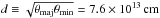 ) and S229.6 GHz = 92 ± 30 mJy, respectively, and those of the additional Gaussian component are 26.0 mas × 23.9 mas (d = 4.1 × 1013 cm) and S229.6 GHz = 59 mJy, respectively. However, significantly different results have been reported by Vlemmings et al. (2015). The elliptical disk component fitted by Vlemmings et al. (2015) has a size of ~43.4 mas × 38.5 mas (d = 6.7 × 1013 cm) and a flux density of S229.6 GHz = 139 ± 0.2 mJy, while the additional Gaussian, which was assumed to be circular in their model, has d = 4.7 mas (0.8 × 1013 cm) and S229.6 GHz = 9.6 ± 0.1 mJy. At 229.6 GHz, the brightness temperature of the 4.7 mas Gaussian component is approximately 10 000 K (Vlemmings et al. 2015), which is much higher than that of the uniform elliptical disk component of Mira A. Vlemmings et al. (2015) therefore argue the existence of a hotspot, or a cluster of unresolved spots, and speculate that its origin may be connected to the stellar magnetic activity of Mira A.
We also conducted a similar continuum analysis of the Mira AB system in ALMA Band 6. In addition to the data in the continuum windows of this SV dataset (spw= 0,7; at 229.6 GHz) as already analysed by Matthews et al. and Vlemmings et al., we also include the continuum data from the six spectral line windows (spw= 1−6 and 8−13). The continuum data in these spectral line windows were prepared by averaging and splitting out the line-free channels in the windows corresponding to each distinct frequency range (see the first two columns of Table A.1), and then exporting the visibility data to Miriad. The visibilities of Mira A and B were fitted simultaneously using the similar model adopted by Matthews et al. (2015) and Vlemmings et al. (2015), i.e. a uniform disk plus an additional Gaussian component for Mira A, and a single Gaussian model for Mira B. We fit the visibilities with the task uvfit (Revision 1.10, 2013 August) in Miriad. Miriad/uvfit is preferred to the uvmodelfit task in CASA because it allows multiple model components to be fitted simultaneously. We cross-checked the uv-fitting results from the respective tasks in Miriad and CASA with single-component models, and both tasks return similar results. To compare the results of Matthews et al. (2015) and Vlemmings et al. (2015), the visibilities of the 229 GHz continuum windows (spw= 0,7) were fitted in a similar manner.
Table A.1 shows the uv-fitting results to the continuum data in the ascending order of the range of rest frequencies. For Mira A, whilst the major and minor axes of the elliptical components appear to be consistent among all spectral windows, the fluxes shared by the uniform disk and the Gaussian component show great variation. The formal errors of the fluxes reported by uvfit are ~9 mJy for the continuum window and 35−40 mJy for the six spectral line windows. Hence, the fitted fluxes of the individual components of Mira A in the line windows are not as reliable as those in the continuum window at 229.6 GHz. Figures A.1 and A.2 show the visibility plots and the maps, respectively, of the fitted continuum models and residuals for all seven continuum and spectral line windows in the Band 6 data. In the maps there are some ~6σ residuals in the 229-GHz continuum window. However, our experiment shows that adding one or two more Gaussian components to the uv-fitting does not significantly improve the results. The residuals in the spectral line windows appear to be less significant than the continuum, probably because the map rms noises are much higher (by a factor of about four) than that in the map of the continuum window.
The size and flux density of our elliptical disk model for Mira A in the continuum window are 51.2 mas × 41.0 mas (d = 7.6 × 1013 cm) and S229.6 GHz = 102 ± 9 mJy. This corresponds to a brightness temperature of 1630 ± 175 K. The uncertainly takes into account the formal errors of the flux (which is the dominant formal error), major and minor axes of the disk model (~0.1 mas), and the bandwidth of the continuum spectral window (~1.7 GHz). The additional Gaussian component for Mira has a size of 26.4 mas × 22.4 mas (d = 4.0 × 1013 cm) and a flux density of S229.6 GHz = 47 ± 9 mJy. These values are consistent with those from Matthews et al. (2015) within uncertainties, but significantly different from the fitting of Vlemmings et al. (2015).
We have tested the uv-fitting model of Vlemmings et al. (2015) in Miriad/uvfit by setting their model parameters for Mira A and B as the initial inputs. Without fixing any parameters, all the fitting trials with Miriad/uvfit eventually converge to our values as presented in Table A.1. The derived major and minor axes of the additional Gaussian component of Mira A are always in the range of ~20−30 mas, which are much larger than 4.7 mas as reported by Vlemmings et al. (2015). On the other hand, even when we fixed the sizes of the uniform disk and Gaussian components to be the same as their values, we were still not able to obtain the same results as in Vlemmings et al. (2015). Figures A.3 (top two panels) and A.4 show the visibility plots and the maps, respectively, in the 229 GHz continuum window of the continuum model and residuals of both Mira A and B using the parameters fitted by Vlemmings et al. (2015). In the model where Mira A was fitted with two components, a uniform disk (UD) and a 4.7 mas Gaussian, we obtain huge residuals that appear to be completely different to the residual image presented in Fig. 1 (right) of Vlemmings et al. (2015). Moreover, in the UD-only model for Mira A (using the best-fit disk model by Vlemmings et al.), we do not obtain the single, compact and bright hotspot near the phase centre as shown in Fig. 1 (middle) of Vlemmings et al. (2015). Instead, we find a pair of strong positive residual features along the SE−NW axis and strong negative features along the SW-NE axis, which may be indicative of an inappropriate shape of the subtracted uniform disk component. We also note that the UD-only residual image of Vlemmings et al. (2015) may show a negative spot in the north-east of the central compact hotspot (their Fig. 1 middle). However, Vlemmings et al. (2015) did not show any negative contour lines or negative colour scale in their figures.
Vlemmings et al. (2015) fitted the continuum visibilities differently from those in Matthews et al. (2015) and from ours in two ways. First, they fitted the continuum dataset of each observing day independently, instead of combing both days together. Second, Vlemmings et al. (2015) used a different uv-fitting tool, UVMULTIFIT, which has been developed by the Nordic ALMA Regional Center Node16 and can be implemented in CASA (Martí-Vidal et al. 2014).
We conducted additional tests to see if we were able to reproduce the fitting results of Vlemmings et al. (2015) by following any one, or both aspects of their approach. Figures A.3 (middle two and bottom two panels) and A.5 show the visibility plots and maps, respectively, of the fitting results using Miriad/uvfit, by splitting the continuum data into individual days of observation. In the fitting, we fixed the sizes and flux densities of the model components of Mira A and B to be the same as used by Vlemmings et al. (2015). The positions of the uniform disk (UD) component of Mira A and the Gaussian component of Mira B were also fixed at the respective stellar positions. The only free parameter in the UD + Gaussian model is therefore the position of the additional Gaussian component of Mira A. Although there are some significant differences between the residual maps on the two observing days, we did not obtain any satisfactory fitting with the parameters obtained by Vlemmings et al. (2015), nor did we find any evidence for the bright spot in the UD-only model. In the UD + Gaussian model for the first day of observation (2014 Oct. 29), we even found the best-fit position of the purported hotspot to be outside the uniform disk component of Mira A, which is far away from the best-fit position as reported by Vlemmings et al. (2015).
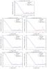 |
Fig. A.1 Visibility plots of the continuum fitting with the task uvfit in Miriad. The plot on the top is the continuum window at 229.6 GHz, and the six below are (from top to bottom, and from left to right) the spectral line windows in ascending order of frequency: 214.0 GHz, 214.3 GHz, 215.5 GHz, 271.1 GHz, 231.8 GHz, 231.6 GHz as listed in Table A.1. The error bars in the continuum window and spectral line windows are 10 times and 1 time, respectively, the standard deviation in the mean of the amplitude of visibilities in the respective bin of uv-distance. The large error bar near 10 Mλ is due to the small number of data points. |
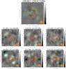 |
Fig. A.2 Continuum fitting results with the task uvfit in Miriad. The large map on the top is the continuum window at 229.6 GHz, the six smaller maps below are (from top to bottom, and from left to right) the spectral line windows in ascending order of frequency: 214.0 GHz, 214.3 GHz, 215.5 GHz, 271.1 GHz, 231.8 GHz, and 231.6 GHz as listed in Table A.1. In all the panels, the orange contours are the continuum models for Mira A, with parameters listed in Table A.1. The sizes of the uniform disk and Gaussian models for the respective spectral windows are shown by blue open ellipses (larger and smaller, respectively). The continuum contour levels are −3,3,10,30,60,120,180,240,300,340 × 0.20 mJy. The green contours and the greyscale maps are the residual images (difference between the data and modelled continuum) of the respective spectral windows. The residual contour levels are −2,2,4,6 × σ, where σ = 0.04 mJy for the continuum window (top) and σ = 0.20 mJy for the six line windows (bottom two rows). The restoring beam of |

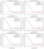 |
Fig. A.3 Visibility plots of the continuum fitting with the task uvfit in Miriad using the parameters obtained by Vlemmings et al. (2015). All the plots are the results of the continuum window at 229.6 GHz. The top panels are the results without splitting the datasets into individual days. The middle and bottom panels are the results of split data for 2014 October 29 and 2014 November 01, respectively. The three panels on the left are the results using uniform disk and a Gaussian to fit Mira A, and the three on the right are the results using only a uniform disk for Mira A. The error bars in the continuum window and spectral line windows are 10 times and 1 time, respectively, the standard deviation in the mean of the amplitude of visibilities in the respective bin of uv-distance. The large error bar near 10 Mλ is due to the small number of data points. |
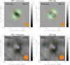 |
Fig. A.4 Results of continuum fitting with the task uvfit in Miriad without splitting the data into two observing days. The top and bottom rows show the results for Mira A and Mira B, respectively. The left column shows the results when Mira A was fitted with a uniform disk and a Gaussian (UD + Gaussian), while the right shows the results when Mira was fitted with the same uniform disk only (UD-only). The parameters for Mira A and B are fixed to those from Vlemmings et al. (2015), except the position of the additional Gaussian component for the UD + Gaussian model of Mira A. The sizes of the uniform disk and Gaussian models for the respective spectral windows are shown by blue open ellipses/circles (larger and smaller, respectively). In all the panels, the orange contour levels for the continuum model are 3,10,30,60,120,180,240,300,360,420, and 540 × 0.20 mJy. The green contours and the greyscale maps are the residual images produced after the modelled continuum visibilities have been subtracted from the respective windows. The residual contour levels for the images of Mira A (top row) are −160,−80,−40,−20,−10,10,20,40, and 80 × σ, and for Mira B (bottom row) are −4,−2,2, and 4 × σ, where σ = 0.04 mJy. The restoring beam of |
Using CASA/UVMULTIFIT (version 2.1.4-r3), we also obtained similar results to those reported above. Assuming that the additional Gaussian component is circular, which is exactly the same model as used by Vlemmings et al. (2015), the size and flux density of the elliptical disk component for Mira A are found to be 50.3 mas × 41.0 mas and S229.6 GHz = 92.9 ± 0.1 mJy, respectively, and those of the additional Gaussian component are 25.4 mas × 25.4 mas and S229.6 GHz = 56.6 ± 0.1 mJy, respectively.
We therefore failed to reproduce any evidence of the compact (<5 mas) Gaussian component in Mira A as suggested by Vlemmings et al. (2015), even if we carried out the fitting using the exact same approach with the same set of model components (elliptical uniform disk + circular Gaussian). Self-calibration may be a possible cause for the discrepancy. However, from their Sect. 2, it is unclear whether Vlemmings et al. (2015) have derived the self-calibration solutions on their own or obtained the solutions from the ALMA Science Portal (as we did). Although Vlemmings et al. (2015) discovered a compact hotspot from their fitting in Band 6, they could not find a similar structure in the continuum data of Band 3 (94.2 GHz) in this ALMA SV dataset with a rms sensitivity of ~40 μJy beam-1. Assuming the size of 4.7 mas and Gaussian brightness distribution, Vlemmings et al. (2015) estimated in their Sect. 4.1.3 the upper limit of the hotspot brightness temperature in Band 3 to be Tb ≲ 17 500 K. However, by repeating the same calculation, we obtained an upper limit of Tb ≲ 250 K, which is a factor of 70 lower than their estimate. Hence we cast doubt on the existence of any detectable compact hotspot near the centre of Mira A’s radio continuum disk near 229 GHz in this ALMA SV data.
Appendix B: A discussion on continuum subtraction in spectral line imaging
It is a standard practice to subtract continuum emission from spectral line data (either from the visibility domain or from the image domain) before image deconvolution (e.g. van Langevelde & Cotton 1990; Thompson et al. 2001, Sect. 11.9). Otherwise, the image deconvolution algorithm (e.g. CLEAN) has to reconstruct a continuum image for each individual, narrowband channel. Because of the non-linear nature of image deconvolution, small differences among channels (such as the frequency-dependent uv-coverage or the noise) may lead to very different convergence of the continuum image (e.g. Cornwell et al. 1992; Rupen 1999, Sect. 6). Further discussions on the necessity of continuum subtraction in spectral line imaging can be found in Sect. 1 of Sault (1994), Sect. 16.9 of the Miriad User Guide17 (version 14 Sept. 2015), and Sect. 8.3 of the  18
18 19 (version 31 Dec. 2015).
B.1. Imaging problem
In our imaging exercises, we find that the images produced from the continuum-subtracted visibility data (hereafter, “continuum-subtracted images/spectra”) and those from the full line and continuum data (hereafter, “full data images/spectra”) are significantly different. Figure B.1 shows the continuum-subtracted spectra of all the observed SiO and H2O lines in ALMA Band 6 extracted from the centre of Mira’s radio continuum. Comparing these spectra to the full data spectra shown in Fig. 8, we expected the only differences to be the trivial constant offsets of about 70−80 mJy/beam, which are the peak radio continuum fluxes of Mira in the respective frequency ranges. In reality, however, the depths of absorption near the systemic velocity channels in the continuum-subtracted spectra are significantly shallower than expected, especially for the vibrational ground state transitions of 28SiO and 29SiO. The effects appear as perplexing bumps near the systemic velocity in the continuum-subtracted spectra. In these velocity channels, bright SiO-emitting clumps and large-scale (≳) SiO emission are present around Mira’s radio photosphere. The discrepancy also appears in the nearby pixels, which show SiO line absorption against the continuum of Mira’s radio photosphere.
In the line-free channels (positive and negative velocity ends of the spectra), the continuum-subtracted spectra have much lower noise than the full data spectra. This is consistent with the fact that CLEAN would introduce additional noise to the image areas where real sources exist (in our case the radio continuum) (see e.g. Sect. 8.3 of the ).
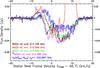 |
Fig. B.1 Spectral lines in ALMA Band 6 extracted from the line of sight towards the centre of Mira’s continuum from the continuum-subtracted maps. The channel maps are presented in Figs. 2−6. The maser emission from SiO ν= 1J = 5−4 transition (in red) above 0.025 Jy is not shown in this figure. |
B.2. Continuum subtraction in the visibility and the image domains
We first compared the imaging results of continuum subtraction in the visibility domain and in the (DIRTY) image domain, using the CASA tasks uvcontsub (then clean) and imcontsub (then deconvolve, which deconvolves the images purely in the image domain), respectively. Both approaches produce the same bumps in the absorption spectra. Hence, we conclude that the discrepancy between the continuum-subtracted and the full data images arises from the image deconvolution (CLEAN) process, but not continuum subtraction.
The following are the two most probable causes of the discrepancy:
-
1.
the full data imaging has failed to recover all SiO line emission,possibly extended, around Mira’s radio photosphere (i.e.missing emission) or, conversely,
-
2.
the continuum-subtracted imaging has failed to recover the correct amount of SiO line absorption against Mira’s radio continuum (i.e. missing absorption).
B.3. Natural weighting versus robust weighting
The first possibility depends on the scales of emission structures and the antenna configuration. In the full data images, all real astrophysical signals would have non-negative fluxes because the continuum emission is included in the data. The strongest line absorption can at most attenuate all the radio flux (i.e. down to zero, but not to a negative value) from the continuum behind the column of gas along the line of sight. In the continuum-subtracted images, on the other hand, strong negative signals would appear in the pixels of Mira’s radio photosphere − representing the line absorption against the continuum − and, strong positive signals would appear around the continuum disk − representing the line-emitting gas outside the radio photosphere. Because of the negative “hole” amidst the positive pixels, any real emission or absorption structures in the continuum-subtracted images would appear to be less extended than those in the full data images. Since the visibility plane sampling (uv-sampling) of ALMA in the long baseline configuration is rather sparse, full data imaging may not be able to recover all possible extended SiO emission from the inner wind of Mira.
Our imaging (Sect. 2) has adopted robust weighting with the parameter ℛBriggs = 0.5. If the “missing emission” scenario is true, then the discrepancy between the continuum-subtracted and the full data spectra should be alleviated under natural weighting, which gives relatively higher weightings to data of short baselines and hence is more sensitive to extended structures. Natural weighting can therefore recover more missing flux (if it exists at all) from the extended SiO emission around the radio photosphere of Mira. Since natural weighting gives a slightly larger synthesised beam than robust weighting, we only compare the maps of CLEAN component (hereafter, CC) models under the two different weighting schemes to eliminate the effect of the beam sizes. We integrate the total flux of the CC models within circles of various spatial scales, centred at Mira’s radio continuum, and obtain the CC spectra of all the images. In contrast to what is expected from the missing emission scenario, we find that the full data CC spectra (not presented) are essentially identical under both weighting schemes. The fact that a higher weighting in short baselines does not recover more fluxes suggests that the ALMA antenna configurations in the SV observation were not missing a significant amount of extended SiO emission from Mira’s inner wind. The absorption profiles of the continuum-subtracted CC spectra, on the other hand, show bumps that are even more prominent under natural weighting than under robust weighting.
In addition to the above test, we also do not expect any missing flux from extended emission structure for two reasons. First, the shortest baseline of this ALMA SV observation is 15 m, corresponding to a maximum recoverable scale20 of over 11″ for the observed SiO transitions, which is at least one order of magnitude larger than the expected SiO depletion radius. Gas density and kinetic temperature also drop rapidly beyond the inner wind of Mira. So we expect the excitation of SiO molecules (both isotopologues) beyond the radius of the detected emission to be varying and very weak. It is unlikely that a smooth and large-scale SiO emission exists, and that the missing flux of which could significantly affect the absorption spectra. Second, negative “bowls” around smaller-scale emission structures, which are characteristic features if smooth extended emission is missing (e.g. Bajaja & van Albada 1979; Braun & Walterbos 1985) are not seen in any of our images.
B.4. Number of CLEAN iterations
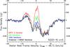 |
Fig. B.2 Continuum-subtracted absorption profiles of the SiO ν= 0J = 5−4 transition along the line of sight towards the centre of Mira’s continuum extracted from images produced by different CLEAN stopping criteria. Images containing the spectra from top to bottom are CLEANed with: 0 iteration (i.e. DIRTY images), 200, 1000, and approximately 18 000 (fully CLEANed to the threshold, see Sect. 2) iterations. |
We therefore consider the second possibility in which the CLEAN process of the continuum-subtracted images may have underestimated the amount of foreground SiO line absorption against the background radio continuum. In order to trace the process of CLEAN iterations and the first batch of CC models selected by the algorithm, we make two additional sets of images, each using a small fixed number of CLEAN iterations instead of an rms noise-dependent threshold as the stopping criteria. Figure B.2 shows the spectra extracted from the images of SiO ν= 0J = 5−4 CLEANed with 200 and 1000 iterations, as well as the spectra from the DIRTY images (no CLEAN iteration) and the fully CLEANed images (down to the threshold value as specified in Sect. 2). In Fig. B.2, the bump feature is seen in all spectra. Its amplitude reaches the maximum in the spectrum extracted from the DIRTY images, and gradually reduces as the number of iterations increases. In general, the DIRTY images are the most severely “corrupted” by the sidelobes of ALMA’s point-spread function (i.e. the DIRTY beam). As CLEAN proceeds to more iterations, the effect of the sidelobes should diminish and eventually vanish below the noise when a low-enough threshold is reached. The apparent resemblance of the bump in the fully CLEANed spectra to that in the DIRTY spectra and the decreasing trend of the bump’s amplitude in the continuum-subtracted spectra with an increasing number of CLEAN iterations seem to suggest that the bump, or excess emission in individual channels, may indeed be the artefacts introduced by the sidelobes of the array’s point-spread function that have not been completely removed by the CLEAN algorithm.
A closer inspection of the 200- and 1000-iteration CC model maps (not presented) shows that the first 1000 CC models selected by the CLEAN algorithm essentially all come from the strong SiO emission in the immediate proximity of Mira’s radio photosphere. Only a handful of negative CC models were found within the radio continuum disk of Mira. We therefore speculate that the initial deconvolution of the strong, extended SiO emission (scales of the order of ) outside the radio continuum may have impaired the subsequent deconvolution of the line absorption within the continuum disk.
B.5. Long-baseline image deconvolution
To examine the performance of image deconvolution when we exclude the contribution from the extended () SiO emission outside Mira’s radio photosphere, another set of continuum-subtracted images are produced for all the observed SiO and H2O lines in Band 6 using only baselines longer than 500 m. The minimum baseline of 500 m corresponds to maximum recoverable scales of about 342−347 mas for the SiO lines, and about 319 mas for the H2O line. In these long-baseline images, the detected flux of the SiO emission around the radio photosphere is significantly reduced or even eliminated. Figure B.3 shows the spectra extracted from the centre of the radio continuum in the long-baseline, continuum-subtracted images. The long-baseline spectra do not show any bumps in the original continuum-subtracted spectra (Fig. B.1), and resemble the similar inverse P Cygni absorption profiles in the full data spectra (Fig. 8). However, the maximum depths of absorption in the long-baseline spectra of the 28SiO and 29SiO ν= 0 transitions appear to be even larger, by about 5 mJy, than the flux level of the radio continuum being absorbed (cf. Fig. 8). We do not have a definitive answer for this “over-absorption” problem. In the long-baseline images, negative bowls are seen at radial distances larger than the SiO emission region. These are the expected characteristic features due to the lack of short baselines (<500 m). The region of the continuum disk amidst the SiO emission is exterior to the “hollow” emission region, and therefore may indeed contain the artefactual negative signals due to the lack of short baselines in addition to the real absorption from the foreground SiO gas.
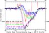 |
Fig. B.3 Spectral lines in ALMA Band 6 extracted from the line of sight towards the centre of Mira’s continuum from the continuum-subtracted maps, only imaged with baselines longer than 500 m. The maser emission from SiO ν= 1J = 5−4 transition (in red) above 0.025 Jy is not shown in this figure. |
B.6. CASA simulation of the ALMA SV observation
Finally, we also simulate the ALMA SV observation of Mira to test whether our preferred model (Sect. 4.4.1), which apparently produces satisfactory fits to the observed full data spectra, can also reproduce the observed bumps in the continuum-subtracted spectra. Positive results would imply that our preferred model can consistently reproduce both the full data and the continuum-subtracted spectra, regardless of the still uncertain causes of the discrepancy in the spectra; negative results, on the other hand, would suggest that our model is still far from approximately describing the structures and physical conditions of Mira’s extended atmosphere and inner wind.
In the CASA simulation task simobserve, we use the sky output model for the 28SiO ν= 0J = 5−4 transition from ratran modelling (Sect. 4) as the input skymodel. For simplicity, we regard the two days of Mira’s SV observation as one continuous observing block in the simulation, and adopt approximate values for the observation parameters. The hour angle at the mid-point of the simulated observation (hourangle) and the total on-source time (totaltime) are set to be −0.8 h and 4000 s, respectively. We also use the actual ALMA antenna configuration in Mira’s SV observation as the input antennalist. Table B.1 lists all 39 ALMA antenna pads (stations) deployed in the SV observation. We note, however, that only 35 or 36 antennae out of 39 were used in each day of observation (ALMA Partnership et al. 2015). Moreover, we did not consider data flagging during the calibration process. These would slightly affect the array’s point-spread function and the map rms noise, but we do not expect a significant deviation from the reality. The longest and shortest baselines also resemble those of the real visibility data. The task simobserve produces a simulated visibility data containing both the continuum and line data (as in our radiative transfer model). We then perform continuum subtraction (with the task uvcontsub) and imaging (with clean) in the exact same ways as for the real data, which are described in Sect. 2.
ALMA antenna pads deployed in Mira’s SV observation.
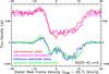 |
Fig. B.4 28SiO ν= 0J = 5−4 spectra extracted from the line of sight towards the centre of Mira’s continuum from the full data images (line+continuum; red and magenta at the top) and from the continuum-subtracted images (blue and green at the bottom). The red and blue spectra correspond to the images from the actual data of Mira’s ALMA SV observation, and the magenta and green spectra correspond to the simulated data using CASA task simobserve. The imaging procedures for the observed and simulated data are identical. |
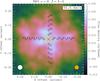 |
Fig. B.5 Same as Fig. 7 for the simulated map of SiO ν= 0J = 5−4 (with the continuum) at the channel of velocity 46.6 km s-1 with a channel width of 1 km s-1. The velocity is slightly different from the systemic velocity of 46.7 km s-1 because of the different velocity grid in our model. The orange contours represent the real data of Mira’s radio continuum at 229 GHz. |
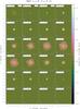 |
Fig. B.6 Same as Fig. 2 for the simulated channel maps of post-imaging continuum-subtracted SiO ν= 0J = 5−4. The white contours represent 6, 12, 18, 24, 48, and 72σ and the yellow contours represent −72, −60, −48, −36, −24, −12, and −6σ, where σ = 0.80 mJy beam-1 is the map rms noise in the real data. The LSR velocities are slightly different from those in Fig. 2 because of the different velocity grid in our model. |
Figure B.4 shows the resultant spectra of the simulation, overlaid with the real spectra as already presented in Figs. 8 (full data) and B.1 (continuum-subtracted). Our simulation successfully reproduces the same bump with the same amplitude (within the noise) and in the same velocity range as in the absorption profile of the continuum-subtracted spectrum. Because this bump is not present in (1) the full data spectrum; (2) the spectrum extracted from modelled images convolved with a circular beam (i.e. the modelled spectrum in the top-left panel of Fig. 10); or (3) our input sky brightness model, we conclude that the bump in the continuum-subtracted spectrum is indeed a spurious feature introduced during the imaging (CLEAN) process. We also suggest that the bump is caused by the missing absorption scenario described in Appendix B. Based on the analyses in the previous sections (Appendices B−B), we speculate that the image deconvolution of the strong SiO emission surrounding the continuum disk, which corresponds to the first batch of the CLEAN component models, has probably impaired the deconvolution of the line absorption region in the images. However, it is still unclear how this has happened, even though CLEAN should be able to handle positive and negative signals equally well. In view of the possible limitations of the CLEAN algorithm, it may be worthwhile to perform imaging tests for this SV data with novel aperture synthesis techniques in radio astronomy (e.g. Sutter et al. 2014; Carrillo et al. 2014; Lochner et al. 2015; Junklewitz et al. 2016).
There are a few other important features in the simulated images and spectra. The noise in the line-free channels of the simulated full data spectrum is comparable to the observed value, and both are significantly higher than the observed/simulated continuum-subtracted spectra. This further supports our earlier claim in Appendix B that CLEANing the radio continuum in individual channels could introduce additional noise to the image products.
We also note that the simulated spectra do not fit well to the observed ones near the velocity of + 10 km s-1. We attribute this to the imperfection of our physical model rather than issues in the data processing (see Sect. 4.4.1).
Our input sky brightness model, which only models the region around Mira up to  and ignores the remote, arc-like emission feature, is spherically symmetric. The modelled
intensity varies smoothly with radius, so it is expected that the simulated images behave in a similar manner. The simulated images, however, contain a lot of clumpy structures that are very similar to what we see in Figs. 2, 3, and 7. Figure B.5 shows the simulated full data image of the SiO ν= 0 line near the systemic velocity, i.e. the channel in which the scale of the SiO emission is the largest. Similar to the same map from the actual observation (Fig. 7), the simulated map also shows structures of enhanced brightness all over the region being modelled. Figure B.6 shows the simulated channel maps of the images, with the continuum subtracted after imaging. These maps also resemble the real data counterpart as shown in Fig. 2: the core SiO line-emitting region appears to be globally spherically symmetric, but it also contains some irregular structures of the similar spatial scales. Qualitatively speaking, the simulated maps are more symmetric and smoother than the real observed maps. The presence of clumpy structures in the simulated images may be due to the sparse uv-sampling of the ALMA long baseline configuration, which makes image deconvolution difficult. In addition, the signal-to-noise ratio may not be sufficient to clearly detect the SiO emission in Mira’s extended atmosphere. Hence, the simulated ALMA observation suggests that the clumpy structures in the extended atmosphere and inner wind of Mira may not be all real.
Appendix C: Full data channel maps (without continuum subtraction)
Figures C.1−C.5 show the channel maps without continuum subtraction. As explained in Sects. 2 and 3.2, we extract from these maps the spectra for our radiative transfer modelling (Sects. 3.3 and 4) and discussion (Sect. 5).
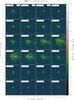 |
Fig. C.1 Same as Fig. 2 for the channel maps, including continuum emission from Mira A, of SiO ν= 0J = 5−4. The absolute position of Mira A is denoted by a black cross. The map rms noise is 0.80 mJy beam-1. In the first panel of the top row, the white box centred at Mira A indicates the |
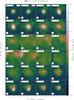 |
Fig. C.2 Same as Fig. C.1 for the zoomed ( |
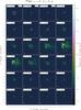 |
Fig. C.3 Same as Fig. C.1 for the channel maps of 29SiO ν= 0J = 5−4 including continuum emission from Mira A. The map rms noise is 0.65 mJy beam-1. |
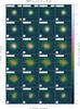 |
Fig. C.4 Same as Fig. C.1 for the zoomed ( |
 |
Fig. C.5 Same as Fig. C.1 for the zoomed ( |
Appendix D: Extrapolation of SiO–H2 collisional rate coefficients
D.1. Pure rotational transitions in the vibrational ground state v = 0
Collisional rate coefficients between SiO and para-H2 (J = 0) are often approximated by scaling the rate coefficients of the SiO−He system by the square root of the ratio of the reduced masses of the two collisional partners, i.e.  (e.g. Schöier et al. 2005). Based on the Gordon-Kim electron gas model (Gordon & Kim 1972), Bieniek & Green (1981) derived the potential energy surface (PES) of the SiO−He system, from which the potential energy of the system in terms of the orientation of the two molecules can be derived (e.g. Lewars 2011, Chap. 2). Bieniek & Green (1983a,b) then computed the collisional cross sections and hence the corresponding rate coefficients for ν≤ 2, J ≤ 39 and Δν = 0,1 for the H2 gas temperature range between 1000 K and 3000 K. Turner et al. (1992) derived the rate coefficients, for ν= 0 and J ≤ 20 only, in a lower temperature range (20−300 K) by extrapolating the PES of Bieniek & Green (1981) to shorter collision distances between SiO and He. With the ab initio method as described in their Sect. 2, Dayou & Balança (2006) have derived a new PES for the SiO−He system which differs significantly from that derived by Bieniek & Green (1981). The resultant rate coefficients from Dayou & Balança (2006) are different from those from Turner et al. (1992) by up to an order of magnitude, with the odd/even-ΔJ propensity rule reversed. The differences are qualitatively similar to the finding by Thomas et al. (1980) that the rate coefficients derived by an electron gas model could be underestimated or overestimated by about 2 to 3 times in the odd- or even-ΔJ transitions, respectively, relative to ab initio calculation. Hence, in our SiO datafile, we adopt the rate coefficients from Dayou & Balança (2006; ν= 0, J ≤ 26) for the collisional transitions of SiO molecule in the vibrational ground state. The rate coefficients for higher J and temperatures are extrapolated by empirically derived analytical approximations as described in the following. For all the function fitting in the following discussion, we use the Levenberg-Marquardt algorithm as the non-linear least squares fitting method. This algorithm is implemented in the Python/SciPy module scipy.optimize.
D.1.1. Extrapolation to high J (Ju> 26)
At the gas temperature T, the collisional rate coefficients, kJuJl, from the initial upper rotational level (Ju) to the final lower level (Jl) in the vibrational ground state (ν= 0) can be computed with the infinite-order sudden approximation (IOS; e.g. Goldflam et al. 1977), 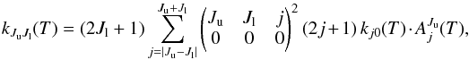 (D.1)where
  (D.2)is the Wigner 3-j symbol. For the special cases in which the bottom three entries of the 3-j symbol equal 0, it has been shown that (e.g. Edmonds 1960; Messiah 1962), if S ≡ ji + jf + j is odd, then
 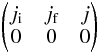 (D.3)and if S ≡ ji + jf + j is even, then
 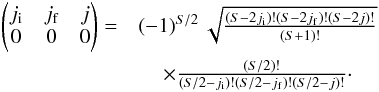 (D.4)The IOS approximation requires that the difference in the rotational energy levels be insignificant to the kinetic energy of the system, which may not be the case for high ΔJ transitions. An adiabaticity factor for purely rotational transitions (i.e. Δν = 0),
  , is therefore required to account for this effect (Ramaswamy et al. 1979; DePristo et al. 1979). The adiabaticity factor at the gas temperature T is given by
  (D.5)where B0 = 0.724 is the rotation constant of SiO (ν= 0) in cm-1, lc ≈ 3 is the typical inelastic impact parameter in Å, and μSiO−H2 = 1.93 is the reduced mass of SiO−H2 in atomic mass unit. To obtain the full set of rate coefficients up to Ju = 69, we need to know the coefficients kj0 for j from 1 up to 137. The SiO−H2 rate coefficients (scaled from SiO−He values) computed by Dayou & Balança (2006) are up to j = 26 only. We extrapolate the coefficients kj0 to higher rotational levels by fitting the Dayou & Balança coefficients to the function
 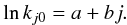 (D.6)The fitting function in Eq. (D.6) does not adopt a second-order term (cj2) as in Schöier et al. (2005) in order to get consistent fitting for all values of temperatures. The values of kj0 become vanishingly small for j ≫ Ju, and hence their contributions to the summation of the coefficient kJuJl are insignificant. Odd and even j are fitted together, so the propensity rule is ignored for the extrapolated j-levels.
However, the rate coefficients computed with Eq. (D.1) and the extrapolated kj0 values are consistently smaller than those theoretically derived by Dayou & Balança (2006). In view of the discrepancy between the Dayou & Balança coefficients and the extrapolated coefficients, we make direct extrapolation of the rate coefficients kJuJl instead of summing up the extrapolated kj0 in Eq. (D.1). For each Jl ≤ 23, we extrapolated kJuJl to higher Ju with 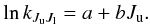 (D.7)For a particular Jl, the variation of the collisional rate coefficients with Ju will then be smoother than in the LAMDA SiO datafile.
D.1.2. Extrapolation to high T
With the J-extrapolated collisional rate coefficients in the temperature range between 10 K and 300 K, we develop the following empirical relation to extrapolate the rate coefficients to higher temperatures:  (D.8)The low-temperature (10−300 K) coefficients of all transitions with the same ΔJ = Ju − Jl are globally fitted to Eq. (D.8) with the same set of fitting parameters mΔJ and nΔJ. The fitting parameters are dependent on ΔJ and their values in units of Kelvin are given in Table D.1. For individual transitions Ju → Jl, we scale the extrapolated coefficient with a factor that ensures continuity with respect to temperature at T = 300 K,
 ![Mathematical equation: \appendix \setcounter{section}{4} \begin{eqnarray} \frac{k^{\rm DB06}_{J_{\rm u}J_{\rm l}} (300\,{\rm K})}{\displaystyle \left( \frac{m_{\Delta J}}{300\,{\rm K}} \right)^{1/4} \exp\left[ -\left( \frac{n_{\Delta J}}{300\,{\rm K}} \right)^{1/4} \right] \times 10^{-10}\,{\rm cm}^{3}\,{\rm s}^{-1}}, \end{eqnarray}](/articles/aa/full_html/2016/06/aa27867-15/aa27867-15-eq543.png) (D.9)where
(D.9)where  is the SiO−H2 rate coefficients (scaled from the SiO−He values) derived by Dayou & Balança (2006) for the transition from Ju to Jl at T = 300 K. Our fitting function in Eq. (D.8) is modified from and has a similar form to the extrapolation functions empirically derived by de Jong et al. (1975), Albrecht (1983), and Bieging et al. (1998), respectively. The extrapolated rate coefficients up to 2000 K are generally consistent with the values in the LAMDA datafile, which are extrapolated by Eq. (13) in Schöier et al. (2005).
Fitting parameters.
D.2. Transitions in the vibrational excited states of SiO
The only available collisional rate coefficients of vibrationally excited SiO in the literature are those derived by Bieniek & Green (1983a,b), based on the old PES model for the SiO−He system and in the temperature range of 1000−3000 K. Thus, for all transitions involving the vibrationally excited states of SiO, we extrapolate from the coefficients of Bieniek & Green (1983a,b; hereafter BG1983 coefficients).
D.2.1 Extrapolation to high-J and high-T
The extrapolation of BG1983 coefficients works on the parameters presented in Table 1 of Bieniek & Green (1983a,b). In their Table 1, the parameters  and
and  from Ji = 0 to 39 are presented, where
  is the rate coefficient from the initial level (νi,Ji) to the ground rotational level of the final vibrational state (νf,0) at T0 = 2000 K, and is the power-law index of the same transition, which describes the temperature dependence of the rate coefficients in the range 1000−3000 K such that
 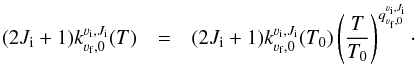 (D.10)We extrapolate the rate coefficient parameters and power-law indices to high-J with approximations similar to Eq. (D.7), i.e.
 ![Mathematical equation: \appendix \setcounter{section}{4} \begin{eqnarray} \ln \left[ (2J_{\rm i}+1) k^{{\varv}_{\rm i},J_{\rm i}}_{{\varv}_{\rm f},0} (T_0) \right] &=& a + b J_{\rm i}, \end{eqnarray}](/articles/aa/full_html/2016/06/aa27867-15/aa27867-15-eq558.png) (D.11)and
(D.11)and 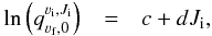 (D.12)except for the rate coefficient parameters of (νi,νf) = (1,0), where we think the parameters are better fitted by a second-order polynomial,
 ![Mathematical equation: \appendix \setcounter{section}{4} \begin{eqnarray} \ln \left[ (2J_{\rm i}+1) k^{{\varv}_{\rm i},J_{\rm i}}_{{\varv}_{\rm f},0} (T_0) \right] &=& a + b J_{\rm i} + c {J_{\rm i}}^2. \end{eqnarray}](/articles/aa/full_html/2016/06/aa27867-15/aa27867-15-eq561.png) (D.13)After the extrapolation, we then compute the full set of rate coefficients at 2000 K,
(D.13)After the extrapolation, we then compute the full set of rate coefficients at 2000 K,  , with the IOS approximation similar to Eq. (D.1), with the only differences being that Ju and Jl in Eq. (D.1) are replaced by Ji (initial level) and Jf (final level), respectively. We only apply the adiabaticity factor (Eq. (D.5)) to the terms within the summation for the pure rotational transition within the same vibrational state, i.e. νi = νf = 1 or 2. For transitions involving a change in the vibrational state, Δν = νi−νf ≠ 0, DePristo et al. (1979) derived a factorisation for the summation terms to correct for the inaccuracy of IOS approximation when the kinetic energy is no longer much greater than the energy of the transition. However, because the rate coefficients are not accurate even with the correction (see our discussion in Appendix D) and the corrected coefficients would not change by many orders of magnitude, we do not think it worthwhile to carry out the factorisation which is quite complicated computationally. So, no adiabaticity correction has been applied to the rate coefficients of transitions with Δν ≠ 0, i.e.
  .
.
Although the power-law indices, , are supposed to be valid only for T = 1000−3000 K, we still adopt the same indices for rate coefficients at T< 1000 K and T> 3000 K because an alternative estimate is not available. New calculations of the collisional rate coefficients for a broad range of kinetic temperatures and for the vibrationally excited states with the updated PES model will be very useful.
D.3. Collisions with rotationally excited H 2
Asymptotic giant branch stars typically have a surface temperature of ~3000 K. In the winds and circumstellar envelopes of these stars, the gas temperature ranges from a few hundred to ≲ 3000 K. Molecular hydrogen in these environments may be significantly populated in the upper rotational levels (e.g. Flower 1989; Doel 1990; Field 1998). For example, the wavelengths of the lowest para-H2 transition, S(0) (Eup/k = 510 K) and the lowest ortho-H2 transition, S(1) (Eup/k = 1015 K) are 28.2 μm and 17.0 μm, respectively (Dabrowski 1984). The approximation of the collisional rate coefficients by the scaled (by ~1.4) coefficients with atomic helium as the collision partner is only valid for the collisions with para-H2 (J = 0), but not for other rotational states of H2 (Field 1998). Lique & Kłos (2008) and Kłos & Lique (2008) have found that the rate coefficients for the collisions between the diatomic molecule SiS with para-H2 (J = 0) are significantly lower than those for the collisions with ortho-H2 (J = 1) or para-H2 (J = 2) by up to an order of magnitude. Similarly, Daniel et al. (2011, and references therein) have also found that the collisions between H2O and rotationally excited H2 in the J = 1 and 2 states are the dominant processes in the collisional (de-)excitation of H2O molecule.
For the SiO molecule, because the currently available collisional rate coefficients do not consider rotationally excited H2 (J = 1 or 2) as the collision partners, the collisional (de-)excitations of SiO in the radiative transfer modelling could well be inaccurate and it is not possible to estimate the errors. In our modelling, it appears that most of the absorption/emission is contributed by the regions which are close to local thermodynamic equilibrium, otherwise there would not be enough absorption along the line of sight towards the continuum or there would be strong maser emission in the SiO ν= 0 and 2 transitions, which show very weak or no maser in the data. So the gas temperature and expansion/infall velocity profiles are probably not affected by the incomplete collisional rate coefficients, but the magnitudes of the H2 gas density and SiO abundance may not be accurate.
Appendix E: Infall-only models
We present here two models, Models 1 and 2, that fail to reproduce the observed SiO and H2O spectra around Mira in ALMA Band 6. Models 1 and 2 exhibit global infall motion only, while our preferred model (Model 3; Sect. 4.4.1) contains a globally expanding layer between the radio photosphere and the globally infalling region.
We first test the infall velocity profiles with monotonically increasing infall velocity (Model 1). Figure E.1 shows the profiles of the gas density (top left), infall velocity (top right), SiO and H2O abundances (middle) and the kinetic temperature (bottom). The bottom row of Fig. E.1 also shows the excitation temperatures of the SiO and H2O transitions (in colour).
Figures E.2−E.4 show our modelled and observed spectra for SiO ν= 0J = 5−4, SiO ν= 2J = 5−4, and H2O v2 = 1JKa,Kc = 55,0−64,3, respectively. The top left panel of these figures show the spectra extracted from the line of sight towards the continuum centre. Although Model 1 may fit well to the redshifted wings (about + 10 to + 15 km s-1) of the SiO spectra, there is significant excess emission from the blueshifted velocities between about −10 and −4 km s-1. The excess blueshifted emission is also seen in the spectra extracted from 32 mas. Additionally, in this spectra extracted from 32 mas, there is an absorption feature against the continuum near the redshifted velocity of about + 10 km s-1, which is not present in the observed spectra.
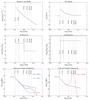 |
Fig. E.1 Inputs for Model 1. Shown in the panels are the H2 gas density (top left), infall velocity (negative represents expansion; top right), 28SiO abundance (middle left), H2O abundance (middle right), and the kinetic temperature (in black) and excitation temperatures (in colours) of the three 28SiO transitions (bottom left) and the H2O transition (bottom right). In the bottom right panel, the solid red line indicates positive excitation temperature (i.e. non-maser emission) of the H2O transition, and the dashed red line indicates the absolute values of the negative excitation temperature (i.e. population inversion) between 1.7 × 10¹⁴ and 2.2 × 1014 cm. Small negative values for the excitation temperature would give strong maser emission. Vertical dotted lines indicate the radii at which the spectra were extracted; coloured horizontal dotted lines in the bottom panels indicates the upper-state energy (Eup/k) of the respective transitions. The innermost layer within Rcontinuum represents the grid cells for the pseudo-continuum, where the input values for H2 gas density and molecular abundances are above the range of the plots. |
 |
Fig. E.2 Model 1: spectra of SiO ν= 0J = 5−4 at various positions. The black histogram is the observed spectrum at the centre of continuum; the green, blue, cyan, and magenta histograms are the observed spectra along the eastern, southern, western, and northern legs, respectively, at various offset radial distances as indicated in each panel. The red curves are the modelled spectra predicted by ratran. |
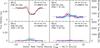 |
Fig. E.3 Model 1: spectra of SiO ν= 2J = 5−4 at various positions. The black histogram is the observed spectrum at the centre of continuum; the green, blue, cyan, and magenta histograms are the observed spectra along the eastern, southern, western, and northern legs, respectively, at various offset radial distances as indicated in each panel. The red curves are the modelled spectra predicted by ratran. |
 |
Fig. E.4 Model 1: spectra of H2O v2 = 1JKa,Kc = 55,0−64,3 at various positions. The black histogram is the observed spectrum at the centre of continuum; the green, blue, cyan, and magenta histograms are the observed spectra along the eastern, southern, western, and northern legs, respectively, at various offset radial distances as indicated in each panel. The red curves are the modelled spectra predicted by ratran. |
As we mention in Sect. 3, the observed weak blueshifted emission feature around the velocities from −10 to −3 km s-1 originates from the emission from the far side of Mira’s extended atmosphere. As the line of sight moves away from the continuum disk, the emission flux of the radio continuum, which is represented by a circular uniform disk in our input model and appears as a flat line in the spectra, falls off rapidly with radius; the flux of the far side molecular emission, on the other hand, decreases more gradually. Hence, the inverse P Cygni profile of the molecular transition emerges from the decreasing continuum level. The blueshifted emission feature in the resultant spectra after beam convolution represents the combined effect of the inner continuum-dominated emission and the outer line-dominated emission. The excess blueshifted emission in Model 1 therefore suggests two possibilities: (1) the gas temperature at the innermost radii in this model is significantly overestimated; and/or (2) this model does not reproduce sufficient absorption in the blueshifted velocities.
For the first postulation, we constructed Model 2, which is identical to Model 1, the only exception being that the gas temperature near the radio photosphere is significantly reduced from 2100 K in the original model to about 1400 K. Figure E.5 shows the input gas temperature and the modelled excitation temperature profiles for the SiO and H2O transitions. Figures E.6−E.8 show the modelled spectra with reduced input gas temperature.
Our modelling results in Figs. E.6−E.8 show that even if we reduce the kinetic temperature to ≲1400 K in the entire inner wind of Mira, there is still an excess in the blueshifted emission. In fact, we have found that the gas temperature near the radio photosphere has to be much lower than 1000 K in order to get rid of this excess emission. In addition, when the kinetic temperature in the proximity of the continuum is reduced, excess absorption relative to the observed spectra would appear in both the SiO and H2O spectra. Although the excess absorption may be compensated by adopting different gas density and molecular abundance profiles, we do not consider the low-temperature atmosphere to be a likely solution.
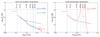 |
Fig. E.5 Input temperature for Model 2. The panels show the kinetic temperature (in black) and excitation temperatures (in colours) of the three 28SiO transitions (left) and the H2O transition (right). In the right panel, the solid red line indicates positive excitation temperature (i.e. non-maser emission) of the H2O transition, and the dashed red line indicates the absolute values of the negative excitation temperature (i.e. population inversion) between 1.7 × 10¹⁴ and 2.4 × 1014 cm. Small negative values for the excitation temperature would give strong maser emission. Vertical dotted lines mark the radii at which the spectra were extracted; coloured horizontal dotted lines in both panels indicates the upper-state energy (Eup/k) of the respective transitions. The innermost layer within Rcontinuum represents the grid cells for the pseudo-continuum. |
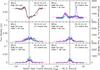 |
Fig. E.6 Model 2: spectra of SiO ν= 0J = 5−4 at various positions. The black histogram is the observed spectrum at the centre of continuum; the green, blue, cyan, and magenta histograms are the observed spectra along the eastern, southern, western, and northern legs, respectively, at various offset radial distances as indicated in each panel. The red curves are the modelled spectra predicted by ratran. |
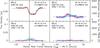 |
Fig. E.7 Model 2: spectra of SiO ν= 2J = 5−4 at various positions. The black histogram is the observed spectrum at the centre of continuum; the green, blue, cyan, and magenta histograms are the observed spectra along the eastern, southern, western, and northern legs, respectively, at various offset radial distances as indicated in each panel. The red curves are the modelled spectra predicted by ratran. |
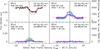 |
Fig. E.8 Model 2: spectra of H2O v2 = 1JKa,Kc = 55,0−64,3 at various positions. The black histogram is the observed spectrum at the centre of continuum; the green, blue, cyan, and magenta histograms are the observed spectra along the eastern, southern, western, and northern legs, respectively, at various offset radial distances as indicated in each panel. The red curves are the modelled spectra predicted by ratran. |
We therefore speculate that in the hot and dense part of the extended atmosphere of Mira (presumably at the innermost radius), there should be a relatively low infall velocity, or even an expanding component contributing to the absorption in the blueshifted part of the spectra. In other words, the infall velocity in the modelled region should not increase monotonically towards the star, but has to decelerate at some radii. In our preferred model (Model 3), we modify the velocity profile such that the motion of the bulk material switches from infall to expansion rapidly at 3.75 × 1013 cm, which is just above our adopted radio photosphere (Rcontinuum = 3.60 × 1013 cm). This expansion zone lies beneath the infall region and hence a large-scale shock of velocity ΔV ≲ 12 km s-1 (constrained by the width of the line profile) could be created near this radius.
All Tables
Photospheric parameters from fitting the continuum visibility data, using the uvfit task in the Miriad software, of Mira A and B in the continuum window at 229.6 GHz of ALMA Band 6.
Photospheric parameters from fitting the continuum visibility data, with the uvfit task in the Miriad software, of Mira A and B in different continuum and spectral line windows of ALMA Band 6.
All Figures
|
Fig. 1 Map of SiO ν= 0J = 5−4 (with the continuum) at the channel of the systemic velocity (46.7 km s-1) with a channel width of 1.0 km s-1. The positions of Mira A (o Ceti; cyan cross) and Mira B (VZ Ceti; yellow cross) are indicated in the image. The horizontal and vertical axes are the relative offsets (arcsec) in the directions of right ascension (X) and declination (Y), respectively, with respect to the continuum centre of Mira A. The white box centred at the fitted position of Mira A indicates the |
| In the text | |
|
Fig. 2 Channel maps of post-imaging continuum-subtracted SiO ν= 0J = 5−4 from LSR velocity 35.7 km s-1 to 58.7 km s-1, with a channel width of 1.0 km s-1. The systemic velocity is 46.7 km s-1. The horizontal and vertical axes indicate the relative offsets (arcsec) in the directions of right ascension (X) and declination (Y), respectively, with respect to the fitted absolute position of Mira A. The white contours represent 6, 12, 18, 24, 48, and 72σ and yellow contours represent −60, −36, and −6σ, where σ = 0.80 mJy beam-1 is the map rms noise. The circular restoring beam of |
| In the text | |
|
Fig. 3 Same as Fig. 2 for the zoomed ( |
| In the text | |
|
Fig. 4 Same as Fig. 2 for the channel maps of post-imaging continuum-subtracted 29SiO ν= 0J = 5−4. The white contours represent 6, 12, 24, 48, 96, and 144σ and yellow contours represent −72, −54, −36, and −6σ, where σ = 0.65 mJy beam-1 is the map rms noise. |
| In the text | |
|
Fig. 5 Same as Fig. 2 for the zoomed ( |
| In the text | |
|
Fig. 6 Same as Fig. 2 for the zoomed ( |
| In the text | |
|
Fig. 7 Map of SiO ν= 0J = 5−4 (with the continuum) at the channel of the systemic velocity (46.7 km s-1) with a channel width of 1 km s-1. The centre of Mira’s continuum is indicated by a black cross. Orange contours represent 10%, 30%, 50%, 70%, and 90% of the peak continuum flux (73.4 mJy beam-1). The black plus signs (+) indicate the positions at which SiO and H2O spectra are sampled and modelled in Sect. 4. The sampling positions are separated by 32 mas along each arm of this array of points. The circular restoring beam of |
| In the text | |
|
Fig. 8 Spectral lines in ALMA Band 6 extracted from the line of sight towards the centre of Mira’s continuum. The SiO ν= 1J = 5−4 transition (in red) shows intense maser emission around + 10 km s-1, with the peak flux density of 1.73 Jy at + 8.8 km s-1. The maser spectrum above 0.10 Jy is not shown in this figure. |
| In the text | |
|
Fig. 9 Inputs of our preferred model. Shown in the panels are the H2 gas density (top left), infall velocity (negative represents expansion; top right), 28SiO abundance (middle left), H2O abundance (middle right), and the kinetic temperature (in black) and excitation temperatures (in colours) of the three 28SiO transitions (bottom left) and the H2O transition (bottom right). In the bottom right panel, the solid red line indicates positive excitation temperature (i.e. non-maser emission) of the H2O transition, and the dashed red line indicates the absolute values of the negative excitation temperature (i.e. population inversion) between 1.7 × 10¹⁴ and 2.4 × 1014 cm. Small negative values for the excitation temperature would give strong maser emission. Vertical dotted lines indicate the radii where the spectra were extracted; coloured horizontal dotted lines in the bottom panels indicates the upper-state energy (Eup/k) of the respective transitions. The innermost layer within Rcontinuum represents the grid cells for the pseudo-continuum, whose input values for H2 gas density and molecular abundances are above the range of the plots. |
| In the text | |
|
Fig. 10 Preferred model: spectra of SiO ν= 0J = 5−4 at various positions. The black histogram is the observed spectrum at the centre of continuum, green, blue, cyan, and magenta histograms are the observed spectra along the eastern, southern, western, and northern legs, respectively, at various offset radial distances as indicated in each panel. The red curves are the modelled spectra predicted by ratran. Our model does not produce the population inversion (i.e. negative excitation temperature) required for maser emission in this SiO transition, so we do not expect our modelled spectra to show any maser emission, as seen in the spike in the upper right panel (see text for the discussion of the spike). |
| In the text | |
|
Fig. 11 Preferred model: spectra of SiO ν= 2J = 5−4 at various positions. The black histogram is the observed spectrum at the centre of continuum, green, blue, cyan, and magenta histograms are the observed spectra along the eastern, southern, western, and northern legs, respectively, at various offset radial distances as indicated in each panel. The red curves are the modelled spectra predicted by ratran. |
| In the text | |
|
Fig. 12 Preferred model: spectra of H2O v2 = 1JKa,Kc = 55,0−64,3 at various positions. The black histogram is the observed spectrum at the centre of continuum, green, blue, cyan, and magenta histograms are the observed spectra along the eastern, southern, western, and northern legs, respectively, at various offset radial distances as indicated in each panel. The red curves are the modelled spectra predicted by ratran, and the blue dashed curves are the same model adopting a high H2O abundance (see the middle right panel of Fig. 9). |
| In the text | |
|
Fig. 13 Spectra of SiO ν= 0J = 5−4 (left) and H2O v2 = 1JKa,Kc = 55,0−64,3 (right) extracted from the centre of the continuum. The black histogram is the observed spectrum and the red curves are the modelled spectra from our preferred model, Model 3. The blue dashed curves are the spectra obtained by reducing the input H2 gas density by a factor of 5; and the green dotted curves are the spectra obtained by increasing the input gas density by a factor of 5 for the modelling of SiO, and a factor of 2 for H2O. |
| In the text | |
|
Fig. 14 Alternative input 28SiO abundance profiles for Model 3 which produce similar modelled spectra. The solid black curve is the same two-step abundance profile as in Model 3, which is close to the minimum possible abundance to fit the ALMA spectra. The three other coloured curves are alternative abundance profiles also using two-step functions. Abundance profile 1 (blue, dashed) has an inner abundance of 1 × 10⁻⁶ up to the radius of ~6 R⋆ and an outer abundance of 1 × 10⁻⁷; profile 2 (green, dash-dotted) has an inner abundance of 8 × 10⁻⁷ up to ~10 R⋆ and an outer abundance of 1 × 10⁻⁸; and profile 3 (red, dotted) has an inner abundance of 1 × 10⁻⁶ up to ~4 R⋆ and an outer abundance of 1 × 10⁻⁷. |
| In the text | |
|
Fig. 15 Preferred model with a layer of an elevated gas temperature. The layer has a width of 2.0 × 1013 cm and an arbitrarily chosen temperature of 4000 K. The left panel shows the elevated gas temperature profiles and the right panel shows the observed and modelled SiO ν= 2J = 5−4 spectra as examples. All other parameters are the same as our preferred model (Model 3). |
| In the text | |
|
Fig. 16 Modified Model 3 with input gas density, kinetic temperature, and velocity profiles from codex models 250420 (top), 261740 (middle), and 286060 (bottom). Special scaling has been applied to the input gas density (see text). The infall velocity profiles are plotted on the left and the selected resultant spectra are shown on the right. We applied constant extrapolation of the infall velocity beyond the outer boundary of codex models. |
| In the text | |
|
Fig. 16 Continued for codex models 287880 (top), 289440 (middle), and 291820 (bottom). |
| In the text | |
|
Fig. 17 Similar to Fig. 16, except that the radius of the pseudo-continuum in the model, Rcontinuum, is changed to 3.65 × 1013 cm for model 250420 (left column) and 3.85 × 1013 cm for model 291820 (right column). The modelled continuum levels are therefore slightly higher than those adopting Rcontinuum = 3.60 × 1013 cm. The strong shock fronts predicted in these two models are hidden inside the radio continuum. The middle and bottom rows show the selected resultant SiO spectra from the corresponding models. |
| In the text | |
|
Fig. 18 Input radial velocity profile (top row) and modelled SiO (middle and bottom rows) spectra of two nearly identical models, except that for the model on the left there is only one large-scale velocity variation close to the radio continuum, while for the model on the right there is an additional strong velocity variation near 1.8 × 1014 cm = 109 mas ~ 5 R⋆. |
| In the text | |
|
Fig. A.1 Visibility plots of the continuum fitting with the task uvfit in Miriad. The plot on the top is the continuum window at 229.6 GHz, and the six below are (from top to bottom, and from left to right) the spectral line windows in ascending order of frequency: 214.0 GHz, 214.3 GHz, 215.5 GHz, 271.1 GHz, 231.8 GHz, 231.6 GHz as listed in Table A.1. The error bars in the continuum window and spectral line windows are 10 times and 1 time, respectively, the standard deviation in the mean of the amplitude of visibilities in the respective bin of uv-distance. The large error bar near 10 Mλ is due to the small number of data points. |
| In the text | |
|
Fig. A.2 Continuum fitting results with the task uvfit in Miriad. The large map on the top is the continuum window at 229.6 GHz, the six smaller maps below are (from top to bottom, and from left to right) the spectral line windows in ascending order of frequency: 214.0 GHz, 214.3 GHz, 215.5 GHz, 271.1 GHz, 231.8 GHz, and 231.6 GHz as listed in Table A.1. In all the panels, the orange contours are the continuum models for Mira A, with parameters listed in Table A.1. The sizes of the uniform disk and Gaussian models for the respective spectral windows are shown by blue open ellipses (larger and smaller, respectively). The continuum contour levels are −3,3,10,30,60,120,180,240,300,340 × 0.20 mJy. The green contours and the greyscale maps are the residual images (difference between the data and modelled continuum) of the respective spectral windows. The residual contour levels are −2,2,4,6 × σ, where σ = 0.04 mJy for the continuum window (top) and σ = 0.20 mJy for the six line windows (bottom two rows). The restoring beam of |
| In the text | |
|
Fig. A.3 Visibility plots of the continuum fitting with the task uvfit in Miriad using the parameters obtained by Vlemmings et al. (2015). All the plots are the results of the continuum window at 229.6 GHz. The top panels are the results without splitting the datasets into individual days. The middle and bottom panels are the results of split data for 2014 October 29 and 2014 November 01, respectively. The three panels on the left are the results using uniform disk and a Gaussian to fit Mira A, and the three on the right are the results using only a uniform disk for Mira A. The error bars in the continuum window and spectral line windows are 10 times and 1 time, respectively, the standard deviation in the mean of the amplitude of visibilities in the respective bin of uv-distance. The large error bar near 10 Mλ is due to the small number of data points. |
| In the text | |
|
Fig. A.4 Results of continuum fitting with the task uvfit in Miriad without splitting the data into two observing days. The top and bottom rows show the results for Mira A and Mira B, respectively. The left column shows the results when Mira A was fitted with a uniform disk and a Gaussian (UD + Gaussian), while the right shows the results when Mira was fitted with the same uniform disk only (UD-only). The parameters for Mira A and B are fixed to those from Vlemmings et al. (2015), except the position of the additional Gaussian component for the UD + Gaussian model of Mira A. The sizes of the uniform disk and Gaussian models for the respective spectral windows are shown by blue open ellipses/circles (larger and smaller, respectively). In all the panels, the orange contour levels for the continuum model are 3,10,30,60,120,180,240,300,360,420, and 540 × 0.20 mJy. The green contours and the greyscale maps are the residual images produced after the modelled continuum visibilities have been subtracted from the respective windows. The residual contour levels for the images of Mira A (top row) are −160,−80,−40,−20,−10,10,20,40, and 80 × σ, and for Mira B (bottom row) are −4,−2,2, and 4 × σ, where σ = 0.04 mJy. The restoring beam of |
| In the text | |
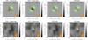 |
Fig. A.5 Same as Fig. A.4 for the fitting results on each day of observation. |
| In the text | |
|
Fig. B.1 Spectral lines in ALMA Band 6 extracted from the line of sight towards the centre of Mira’s continuum from the continuum-subtracted maps. The channel maps are presented in Figs. 2−6. The maser emission from SiO ν= 1J = 5−4 transition (in red) above 0.025 Jy is not shown in this figure. |
| In the text | |
|
Fig. B.2 Continuum-subtracted absorption profiles of the SiO ν= 0J = 5−4 transition along the line of sight towards the centre of Mira’s continuum extracted from images produced by different CLEAN stopping criteria. Images containing the spectra from top to bottom are CLEANed with: 0 iteration (i.e. DIRTY images), 200, 1000, and approximately 18 000 (fully CLEANed to the threshold, see Sect. 2) iterations. |
| In the text | |
|
Fig. B.3 Spectral lines in ALMA Band 6 extracted from the line of sight towards the centre of Mira’s continuum from the continuum-subtracted maps, only imaged with baselines longer than 500 m. The maser emission from SiO ν= 1J = 5−4 transition (in red) above 0.025 Jy is not shown in this figure. |
| In the text | |
|
Fig. B.4 28SiO ν= 0J = 5−4 spectra extracted from the line of sight towards the centre of Mira’s continuum from the full data images (line+continuum; red and magenta at the top) and from the continuum-subtracted images (blue and green at the bottom). The red and blue spectra correspond to the images from the actual data of Mira’s ALMA SV observation, and the magenta and green spectra correspond to the simulated data using CASA task simobserve. The imaging procedures for the observed and simulated data are identical. |
| In the text | |
|
Fig. B.5 Same as Fig. 7 for the simulated map of SiO ν= 0J = 5−4 (with the continuum) at the channel of velocity 46.6 km s-1 with a channel width of 1 km s-1. The velocity is slightly different from the systemic velocity of 46.7 km s-1 because of the different velocity grid in our model. The orange contours represent the real data of Mira’s radio continuum at 229 GHz. |
| In the text | |
|
Fig. B.6 Same as Fig. 2 for the simulated channel maps of post-imaging continuum-subtracted SiO ν= 0J = 5−4. The white contours represent 6, 12, 18, 24, 48, and 72σ and the yellow contours represent −72, −60, −48, −36, −24, −12, and −6σ, where σ = 0.80 mJy beam-1 is the map rms noise in the real data. The LSR velocities are slightly different from those in Fig. 2 because of the different velocity grid in our model. |
| In the text | |
|
Fig. C.1 Same as Fig. 2 for the channel maps, including continuum emission from Mira A, of SiO ν= 0J = 5−4. The absolute position of Mira A is denoted by a black cross. The map rms noise is 0.80 mJy beam-1. In the first panel of the top row, the white box centred at Mira A indicates the |
| In the text | |
|
Fig. C.2 Same as Fig. C.1 for the zoomed ( |
| In the text | |
|
Fig. C.3 Same as Fig. C.1 for the channel maps of 29SiO ν= 0J = 5−4 including continuum emission from Mira A. The map rms noise is 0.65 mJy beam-1. |
| In the text | |
|
Fig. C.4 Same as Fig. C.1 for the zoomed ( |
| In the text | |
|
Fig. C.5 Same as Fig. C.1 for the zoomed ( |
| In the text | |
|
Fig. E.1 Inputs for Model 1. Shown in the panels are the H2 gas density (top left), infall velocity (negative represents expansion; top right), 28SiO abundance (middle left), H2O abundance (middle right), and the kinetic temperature (in black) and excitation temperatures (in colours) of the three 28SiO transitions (bottom left) and the H2O transition (bottom right). In the bottom right panel, the solid red line indicates positive excitation temperature (i.e. non-maser emission) of the H2O transition, and the dashed red line indicates the absolute values of the negative excitation temperature (i.e. population inversion) between 1.7 × 10¹⁴ and 2.2 × 1014 cm. Small negative values for the excitation temperature would give strong maser emission. Vertical dotted lines indicate the radii at which the spectra were extracted; coloured horizontal dotted lines in the bottom panels indicates the upper-state energy (Eup/k) of the respective transitions. The innermost layer within Rcontinuum represents the grid cells for the pseudo-continuum, where the input values for H2 gas density and molecular abundances are above the range of the plots. |
| In the text | |
|
Fig. E.2 Model 1: spectra of SiO ν= 0J = 5−4 at various positions. The black histogram is the observed spectrum at the centre of continuum; the green, blue, cyan, and magenta histograms are the observed spectra along the eastern, southern, western, and northern legs, respectively, at various offset radial distances as indicated in each panel. The red curves are the modelled spectra predicted by ratran. |
| In the text | |
|
Fig. E.3 Model 1: spectra of SiO ν= 2J = 5−4 at various positions. The black histogram is the observed spectrum at the centre of continuum; the green, blue, cyan, and magenta histograms are the observed spectra along the eastern, southern, western, and northern legs, respectively, at various offset radial distances as indicated in each panel. The red curves are the modelled spectra predicted by ratran. |
| In the text | |
|
Fig. E.4 Model 1: spectra of H2O v2 = 1JKa,Kc = 55,0−64,3 at various positions. The black histogram is the observed spectrum at the centre of continuum; the green, blue, cyan, and magenta histograms are the observed spectra along the eastern, southern, western, and northern legs, respectively, at various offset radial distances as indicated in each panel. The red curves are the modelled spectra predicted by ratran. |
| In the text | |
|
Fig. E.5 Input temperature for Model 2. The panels show the kinetic temperature (in black) and excitation temperatures (in colours) of the three 28SiO transitions (left) and the H2O transition (right). In the right panel, the solid red line indicates positive excitation temperature (i.e. non-maser emission) of the H2O transition, and the dashed red line indicates the absolute values of the negative excitation temperature (i.e. population inversion) between 1.7 × 10¹⁴ and 2.4 × 1014 cm. Small negative values for the excitation temperature would give strong maser emission. Vertical dotted lines mark the radii at which the spectra were extracted; coloured horizontal dotted lines in both panels indicates the upper-state energy (Eup/k) of the respective transitions. The innermost layer within Rcontinuum represents the grid cells for the pseudo-continuum. |
| In the text | |
|
Fig. E.6 Model 2: spectra of SiO ν= 0J = 5−4 at various positions. The black histogram is the observed spectrum at the centre of continuum; the green, blue, cyan, and magenta histograms are the observed spectra along the eastern, southern, western, and northern legs, respectively, at various offset radial distances as indicated in each panel. The red curves are the modelled spectra predicted by ratran. |
| In the text | |
|
Fig. E.7 Model 2: spectra of SiO ν= 2J = 5−4 at various positions. The black histogram is the observed spectrum at the centre of continuum; the green, blue, cyan, and magenta histograms are the observed spectra along the eastern, southern, western, and northern legs, respectively, at various offset radial distances as indicated in each panel. The red curves are the modelled spectra predicted by ratran. |
| In the text | |
|
Fig. E.8 Model 2: spectra of H2O v2 = 1JKa,Kc = 55,0−64,3 at various positions. The black histogram is the observed spectrum at the centre of continuum; the green, blue, cyan, and magenta histograms are the observed spectra along the eastern, southern, western, and northern legs, respectively, at various offset radial distances as indicated in each panel. The red curves are the modelled spectra predicted by ratran. |
| In the text | |
Current usage metrics show cumulative count of Article Views (full-text article views including HTML views, PDF and ePub downloads, according to the available data) and Abstracts Views on Vision4Press platform.
Data correspond to usage on the plateform after 2015. The current usage metrics is available 48-96 hours after online publication and is updated daily on week days.
Initial download of the metrics may take a while.