| Issue |
A&A
Volume 566, June 2014
|
|
|---|---|---|
| Article Number | A150 | |
| Number of page(s) | 30 | |
| Section | Interstellar and circumstellar matter | |
| DOI | https://doi.org/10.1051/0004-6361/201423420 | |
| Published online | 26 June 2014 | |
A multiple system of high-mass YSOs surrounded by disks in NGC 7538 IRS1
Gas dynamics on scales of 10–700 AU from CH3OH maser and NH3 thermal lines⋆
1
INAF – Osservatorio Astrofisico di Arcetri, Largo E. Fermi 5
50125
Firenze,
Italy
e-mail:
mosca@arcetri.astro.it
2
Joint Institute for VLBI in Europe, Postbus 2, 7990 AA
Dwingeloo, The
Netherlands
e-mail:
goddi@jive.nl
Received:
14
January
2014
Accepted:
14
April
2014
Context. It has been claimed that NGC 7538 IRS1 is a high-mass young stellar object (YSO) with 30 M⊙, surrounded by a rotating Keplerian disk, probed by a linear distribution of methanol masers. The YSO is also powering a strong compact Hii region or ionized wind, and is driving at least one molecular outflow. The axis orientations of the different structures (ionized gas, outflow, and disk) are, however, misaligned, which has led to the different competing models proposed to explain individual structures.
Aims. We investigate the 3D kinematics and dynamics of circumstellar gas with very high linear resolution, from tens to 1500 AU, with the ultimate goal of building a comprehensive dynamical model for what is considered the best high-mass accretion disk candidate around an O-type young star in the northern hemisphere.
Methods. We used high-angular resolution observations of 6.7 GHz CH3OH masers with the EVN, NH3 inversion lines with the JVLA B-Array, and radio continuum with the VLA A-Array. In particular, we employed four different observing epochs of EVN data at 6.7 GHz, spanning almost eight years, which enabled us to measure line-of-sight (l.o.s.) accelerations and proper motions of CH3OH masers, besides l.o.s. velocities and positions (as done in previous works). In addition, we imaged highly excited NH3 inversion lines, from (6,6) to (13,13), which enabled us to probe the hottest molecular gas very close to the exciting source(s).
Results. We confirm previous results that five 6.7 GHz maser clusters (labeled from “A” to “E”) are distributed over a region extended N–S across ≈1500 AU, and are associated with three components of the radio continuum emission. We propose that these maser clusters identify three individual high-mass YSOs in NGC 7538 IRS1, named IRS1a (associated with clusters “B” and “C”), IRS1b (associated with cluster “A”), and IRS1c (associated with cluster “E”). We find that the 6.7 GHz masers distribute along a line, with a regular variation in VLSR with position, along the major axis of the distribution of maser cluster “A” and the combined clusters “B” + “C”. A similar VLSR gradient (although shallower) is also detected in the NH3 inversion lines. Interestingly, the variation in VLSR with projected position is not linear but quadratic for both maser clusters. We measure proper motions for 33 maser features, which have an average amplitude (4.8 ± 0.6 km s-1) similar to the variation in VLSR across the maser cluster, and are approximately parallel to the clusters’ elongation axes. By studying the time variation in the maser spectrum, we also derive l.o.s. accelerations for 30 features, with typical amplitude of ~ 10-3−10-2 km s-1 yr-1. We modeled the masers in both clusters “A” and “B” + “C” in terms of an edge-on disk in centrifugal equilibrium. Based on our modeling, masers of clusters “B” + “C” may trace a quasi-Keplerian ~1 M⊙, thin disk, orbiting around a high-mass YSO, IRS1a, of up to ≈25 M⊙. This YSO dominates the bolometric luminosity of the region. The disk traced by the masers of cluster “A” is both massive (≲16 M⊙ inside a radius of ≈500 AU) and thick (opening angle ≈45°), and the mass of the central YSO, IRS1b, is constrained to be at most a few M⊙. Towards cluster “E”, NH3 and 6.7 GHz masers trace more quiescent dynamics than for the other clusters. The presence of a radio continuum peak suggests that the YSO associated with the cluster “E”, IRS1c, may be an ionizing, massive YSO as well.
Conclusions. We present compelling evidence that NGC 7538 IRS1 is forming not just one single high-mass YSO, but consists of a multiple system of high-mass YSOs, which are surrounded by accretion disks and are probably driving individual outflows. This new model naturally explains all the different orientations and disk/outflow structures proposed for the region in previous models.
Key words: ISM: jets and outflows / ISM: molecules / masers / accretion, accretion disks / techniques: interferometric
Table 2 and Appendix A are available in electronic form at http://www.aanda.org
© ESO, 2014
1. Introduction
The formation of massive stars (O-B type) by the same accretion processes believed to form low-mass stars appears problematic, because the intense radiation pressure from the star luminosity and the thermal pressure from the Hii region around the young stellar objects (YSOs) may be sufficient to reverse the accretion flow and prevent matter from reaching the star (Zinnecker & Yorke 2007). The “standard” theory predicts that this occurs for stars having masses in excess of 8 M⊙, leading to the paradoxical conclusion that stars above this limit should not exist (Palla & Stahler 1993). Recent theories have demonstrated that the radiation pressure problem can be solved if accretion occurs through a circumstellar disk (e.g., Kuiper et al. 2010, 2011), thus explaining the formation of stars up to 140 M⊙. In a very different scenario, Bonnell et al. (1998) proposed that O-type stars may form through the merger of low-mass objects. While a handful of disk candidates in B-type (M⋆< 20M⊙) protostars has been reported in the literature in recent years (Cesaroni et al. 2006, and references therein), there has been no clear evidence of accretion disks around more massive O-type stars so far. The few rotating molecular structures detected around O-type stars (on scales >10 000 AU) have been interpreted as gravitationally unstable, transient bodies, infalling and accreting either to a central cluster of low-mass protostars (Sollins & Ho 2005; Beltrán et al. 2011) or to a single massive protostar (Sandell et al. 2003; Beuther & Walsh 2008). Since O-type stars form at large distances (a few kpc) and deeply embedded inside dense massive cores (likely containing protoclusters), both confusion/crowding and poor resolution in previous studies have precluded distinguishing between different star formation scenarios and, ultimately, establishing whether the rotating and infalling material in the cloud actually accretes onto individual massive protostars. This would require resolving the structure and dynamics of accreting gas at small radii (≲1000 AU) from massive YSOs, but this has been challenging so far (present millimeter interferometers have typical resolutions on the order of 1′′, corresponding to 1000 AU at 1 kpc). Therefore, observational signatures of rotating disks around O-type forming stars are essential to progressing in our understanding of the mass-accretion process and to constraining theoretical models of high-mass star formation.
In this context, one excellent diagnostic tool of gas kinematics within 10–1000 AU from YSOs is provided by multi-epoch very long baseline interferometric (VLBI) observations of interstellar masers (Goddi & Moscadelli 2006; Goddi et al. 2006, 2011; Matthews et al. 2010; Moscadelli et al. 2007, 2011, 2013; Sanna et al. 2010a,b; Torrelles et al. 2003, 2011). Among different molecular masers, CH3OH is particularly interesting, because it is exclusively associated with high-mass star formation and provides an excellent probe of accretion. Recently, Goddi et al. (2011) have reported a convincing signature of infall in a circumstellar molecular envelope with a radius of only 300 AU around a B-type forming star in AFGL 5142, by using multi-epoch VLBI observations of CH3OH masers spanning six years. Measurements of the 3D velocity field of the circumstellar gas has provided the most direct and least unbiased measurement (yet obtained) of infall of a molecular envelope onto an intermediate- to high-mass protostar. Other interesting examples of 3D kinematics with methanol masers are reported in Sanna et al. (2010a,b) and Moscadelli et al. (2011, 2013).
To characterize the accretion process in an O-type YSO, we study one of the best high-mass accretion disk candidates in the northern hemisphere, NGC 7538 IRS1. This region is relatively nearby (2.7 kpc; Moscadelli et al. 2009), very luminous (~105L⊙; e.g., Akabane & Kuno 2005), it contains an Hii region (e.g., Wynn-Williams et al. 1974), and it has been suggested to be powered by an O6/7 star of about 30 M⊙. Very Large Array (VLA) continuum observations revealed a double-peaked structure in the ionized gas within 0.̋2 from the central core and a more extended (~1′′) emission elongated N–S (e.g., Gaume et al. 1995). Radio recombination lines observed at cm- and mm-wavelengths show extremely broad line widths, suggestive of expanding motions of the ionized gas (Gaume et al. 1995; Keto et al. 2008). A multi-wavelength study of the radio continuum showed that the free-free emission from IRS1 is dominated by an ionized jet, rather than a hyper-compact H ii region (Sandell et al. 2009). Recently, a number of interferometric studies conducted with increasing angular resolution, at 1.3 mm with the SMA (3′′ beamsize, Qiu et al. 2011), at 1.3 and 3.4 mm with the SMA and CARMA (0.̋7 beamsize, Zhu et al. 2013), and at 0.8 mm with the PdBI (0.̋2 beamsize, Beuther et al. 2013), detected several typical hot-core species, showing inverse P-Cygni profiles, probing inward motion of the dense gas on scales ≳1000 AU with a mass infall rate Ṁ ~ 10-3M⊙ yr-1. These radio centimeter and millimeter observations also identified several outflows emanating from NGC 7538 IRS1, along N–S (Gaume et al. 1995; Sandell et al. 2009), NW–SE (Qiu et al. 2011), and NE–SW (Beuther et al. 2013). The simultaneous presence of jets/outflows and a strong accretion flow toward IRS 1, led some authors to postulate the presence of an accretion disk surrounding IRS 1. Minier et al. (1998) observed a linear distribution of 6.7 and 12.2 GHz CH3OH masers with a position angle (PA) of about 112° and Pestalozzi et al. (2004) proposed an edge-on Keplerian disk model to explain positions and l.o.s. velocities of maser spots. A mid-infrared (IR) study however questioned the edge-on disk model traced by the CH3OH masers, suggesting that the radio continuum emission (elongated N–S) traces an ionized wind emanating from the surface of a disk with PA of ~30° perpendicular to the NW–SE CO-bipolar outflow (De Buizer & Minier 2005). In an attempt to explain the different orientation of the elongated structures observed in the CH3OH masers and in the near-IR emission, Kraus et al. (2006) proposed that the edge-on disk is driving a precessing jet. Surcis et al. (2011) however pointed out that, in addition to the linear CH3OH maser cluster proposed to trace the edge-on Keplerian disk, there are additional maser clusters in the region within 1′′, and they proposed an alternative scenario where all the observed CH3OH maser clusters should mark the interface between the infalling envelope and a large-scale torus, having a rotation axis with the same PA (≈–45°) of the elongated mid-IR emission observed by De Buizer & Minier (2005).
6.7 GHz CH3OH maser EVN observations.
While the individual competing models explain some properties of the system, either the ordered structure of one maser cluster (e.g., Pestalozzi et al. 2004), or the global spatial distribution of all clusters (e.g., Surcis et al. 2011), or the complex pattern of molecular outflows emerging from IRS 1 (Kraus et al. 2006), they fail to provide a clear picture of accretion/outflow in terms of a simple disk/jet system, as expected in the context of a canonical picture of star formation. Likewise, despite the plethora of interferometric studies on the region at (sub)mm-wavelengths (with angular resolutions in the range 0.̋2–2′′), no clear evidence of a rotating disk has been found and only a confusing picture for the outflows has been drawn so far.
In this paper, we overcome the shortcomings of previous works by analyzing a multi-epoch dataset of 6.7 GHz CH3OH maser observations and complementing the maser data with new interferometric images of highly excited inversion lines of NH3, from (6,6) to (13,13). This approach has a two-fold advantage. First, the multi-epoch dataset (spanning almost eight years), enables us to measure proper motions and l.o.s. accelerations of CH3OH masers, besides positions and l.o.s. velocities (as done in previous works). Second, highly excited inversion lines of NH3 at cm-wavelengths, enable us to probe the hottest gas close the YSO(s) in an optically thin regime and at the highest angular resolutions achievable with connected-element interferometers (previous works were conducted at mm-wavelengths and/or with poorer angular resolutions). A detailed analysis of the NH3 data will be presented in a forthcoming paper (Goddi et al. in prep.). The main goal of this paper is to investigate the 3D dynamics of the circumstellar molecular gas at the small scales (10–500 AU) probed by the masers and relates it to the large-scale motions (500–2000 AU) probed by the complementary interferometric thermal NH3 data.
We describe observations and data reduction in Sect. 2 and our observational results in Sect. 3. In Sect. 4, we examine the ordered velocity structures measured with the CH3OH masers and thermal NH3 lines. We present a dynamical model to explain our measurements in Sect. 5, followed by a discussion on the nature of star formation in NGC 7538 IRS1 in Sect. 6. Some implications of our model and a comparison with previous models are illustrated in Sect. 7. Finally, we summarize our main findings in Sect. 8.
2. Observations
2.1. EVN 6.7 GHz CH3OH maser archival observations
This work is based on archival data of 6.7 GHz CH3OH masers observed towards NGC 7538 IRS1 with the European VLBI Network (EVN1). In particular, we reduced and analyzed four individual datasets at four distinct observing epochs over the years 2002–2009. For each observation, Table 1 reports the observing date, the angular and velocity resolution, and the sensitivity of the reconstructed maser images. The reduced sensitivity of the 2002 February run (EVN code: EP039B) is due to the lower number of observing antennae (six: Jodrell, Cambridge, Effelsberg, Medicina, Torun and Onsala) compared with the subsequent runs, which employed either eight (EC021 and EP054: including also Noto and Westerbork) or nine (ES063B: including also Yebes) telescopes. Details of the observational setup of ES063B can be found in Surcis et al. (2011).
Data were reduced with the NRAO Astronomical Image Processing System (AIPS) package, following the VLBI spectral line procedures. The time persistent emission of the strongest maser channel (corresponding to feature #1 in Table 2) has been self-calibrated and the complex gain corrections have been applied to all the emission channels before imaging. Maser images cover a field of view, Δα×Δδ ≈ 8″ × 8″, and a VLSR range, from −71 km s-1 to −52 km s-1, adequate to recover all the 6.7 GHz maser emission previously detected towards NGC 7538 IRS1. For a description of the criteria used to identify individual masing clouds, derive their parameters (position, intensity, flux and size), and measure their relative proper motions, we refer to Sanna et al. (2010a). In the following we use the term “spot” to indicate a compact emission centre on a single-channel map, and the term “feature” to refer to a collection of spots emitting in contiguous channels at approximately the same position in the sky (within the beam FWHM).
Since none of the four EVN runs was observed in phase-reference mode, no accurate
information on the absolute position of the 6.7 GHz CH3OH masers can be derived
directly from these data. However, Minier et al.
(1998) and Pestalozzi et al. (2004) have
shown that there is a good correspondence in position and VLSR between the
6.7 GHz and 12 GHz methanol masers in NGC 7538 IRS1. In particular, the strongest features
of both maser transitions have an elongated structure (cluster “A”, see Sect 3.1.1), and the agreement between 6.7 GHz and 12.2 GHz
masers is within a few mas in relative position and 0.1 km s-1 in VLSR. For the
12.2 GHz methanol masers, Moscadelli et al. (2009)
determined the absolute position (RA(J2000) = 23h 13m 45 3622 , Dec
(J2000) = 61°28′ 10.̋507) and the apparent proper motion (μRA = −2.45 mas
yr-1,
μDec =
−2.45 mas yr-1) with high accuracy using multi-epoch, phase-referencing
observations with the Very Long Baseline Array (VLBA). In the assumption that the most
intense 6.7 and 12 GHz maser features are spatially coincident, we can then determine the
absolute position of the 6.7 GHz masers with milliarcsecond accuracy as well. As a
comparison, our derivation of the absolute position of the 6.7 GHz masers in NGC 7538 IRS1
agrees with that determined by Surcis et al. (2011)
using Multi-Element Radio Linked Interferometer network (MERLIN) observations within their
measurement error of 10 mas.
3622 , Dec
(J2000) = 61°28′ 10.̋507) and the apparent proper motion (μRA = −2.45 mas
yr-1,
μDec =
−2.45 mas yr-1) with high accuracy using multi-epoch, phase-referencing
observations with the Very Long Baseline Array (VLBA). In the assumption that the most
intense 6.7 and 12 GHz maser features are spatially coincident, we can then determine the
absolute position of the 6.7 GHz masers with milliarcsecond accuracy as well. As a
comparison, our derivation of the absolute position of the 6.7 GHz masers in NGC 7538 IRS1
agrees with that determined by Surcis et al. (2011)
using Multi-Element Radio Linked Interferometer network (MERLIN) observations within their
measurement error of 10 mas.
The EVN experiment EP039B (labeled “0” in Table 1) resulted in less sensitive images, and only a few, intense (≥1 Jy beam-1), 6.7 GHz maser features could be detected. Maser proper motions have been derived using merely the subsequent three, more sensitive epochs (labeled 1–3 in Table 1), showing similar (naturally weighted) beams. In the following analysis, epoch “0” data are employed only to extend the time baseline and calculate the l.o.s. accelerations of the most intense maser features with higher accuracy (see Sect. 3.1.2).
2.2. VLA archival observations
Gaume et al. (1995) used the VLA in the most extended A-configuration to observe the H66α line (at 22364.174 MHz) towards NGC 7538 IRS1 on 1992 December 12 and 20 (exp. code: AG360). We downloaded the data of this observation from the VLA archive and, following Gaume et al. (1995), derived the continuum emission as the “channel zero” data, by averaging the inner 75% of the 25 MHz observing band. Data have been calibrated following the standard procedure for VLA continuum data, as also described in Gaume et al. (1995). The continuum map, produced using uniform-weighting, has a FWHM beam of 0.̋077 × 0.̋074 with PA = 90°. We precessed the coordinate system of the continuum map from the B1950 to the J2000 equatorial system, and we also corrected for the apparent motion between the VLA observing epoch, December 1992, and the first epoch, September 2005, of the 12.2 GHz CH3OH maser VLBA observations.
2.3. NH3 JVLA observations
Observations of NH3 towards NGC 7538 IRS1 were conducted using the Karl G. Jansky Very Large Array (JVLA) of the National Radio Astronomy Observatory (NRAO)2 in B configuration. By using the broadband JVLA K- and Ka-band receivers, we observed a total of five metastable inversion transitions of NH3: (J,K) = (6,6), (7,7), (9,9), (10,10), (13,13) at 1.3 cm, with frequencies going from ≈25.1 GHz for the (6,6) line to ≈33.2 GHz for the (13,13) line. Transitions were observed in pairs of (independently tunable) basebands during 6 h tracks (two targets per track) on three different dates in 2012: the (6,6) and (7,7) lines on May 31 at K-band, the (9,9) and (13,13) lines on June 21, and the (10,10) transition on August 7, at Ka-band. Each baseband had eight sub-bands with a 4 MHz bandwidth per sub-band (≈40 km s-1 at 30 GHz), providing a total coverage of 32 MHz (≈320 km s-1 at 30 GHz). Each sub-band consisted of 128 channels with a separation of 31.25 kHz (≈0.4 km s-1 at 30 GHz). Typical on-source integration time was 53 min. Each transition was observed with “fast switching”, where 60 s scans on-target were alternated with 60 s scans of the nearby (3° on the sky) QSO J2339+6010 (measured flux density Fν = 0.2–0.3 Jy, depending on frequency). We derived absolute flux calibration from observations of 3C 48 (Fν = 0.5–0.7 Jy, depending on frequency), and bandpass calibration from observations of 3C 84 (Fν = 24–28 Jy, depending on frequency).
The data were edited, calibrated, and imaged in a standard fashion using the Common
Astronomy Software Applications (CASA) package. We fitted and subtracted continuum
emission from the spectral line data in the uv plane using CASA task UVCONTSUB, combining
the continuum (line-free) signal from all eight sub-bands around the NH3 line. Before imaging the
NH3 lines, we
performed self-calibration of the continuum emission. The continuum images showed an
integrated flux density and a 1σ rms varying in the range 400–600 mJy and 80–240
μJy
beam-1, from 25
to 33 GHz, respectively. We then applied the self-calibration solutions from the continuum
to the line datasets. Using the CASA task CLEAN, we imaged the NGC 7538 region with a cell
size of 0.̋04, covering an 8′′ field around the phase-centre position:
 , δ(J2000) = +
61°28′10″. We adopted Briggs weighting with a
ROBUST parameter set to 0.5 and smoothed the velocity resolution to 0.4 km
s-1 for all
transitions. The resulting synthesized clean beam FWHM was 0.̋15–0.̋27 and the rms noise
level per channel was ≈1.5–2.5
mJy beam-1,
depending on frequency.
, δ(J2000) = +
61°28′10″. We adopted Briggs weighting with a
ROBUST parameter set to 0.5 and smoothed the velocity resolution to 0.4 km
s-1 for all
transitions. The resulting synthesized clean beam FWHM was 0.̋15–0.̋27 and the rms noise
level per channel was ≈1.5–2.5
mJy beam-1,
depending on frequency.
Since the position of the phase calibrator, J2339+6010, was only accurate within 0.′′15, according to the The VLA Calibrator Manual3, we conducted a 30 m test in December 2013 to check the astrometry of our NH3 maps, observing J2339+6010 and NGC 7538 in fast-switching with QSO J2230+6946. We measured a positional offset of Δα ~ −0.′′01, Δδ ~ 0.′′16 from the nominal position of J2339+6010 reported in the VLA catalog. All the NH3 maps of NGC 7538 IRS1 reported in this paper were shifted accordingly by the measured offset. For the sake of comparison with the VLBI CH3OH maps, we also corrected for the apparent motion between December 2013, and the first epoch, September 2005, of the 12.2 GHz CH3OH maser VLBA observations (as done for the radio continuum image).
3. Results
We discuss here gas dynamics in NGC 7538 IRS1 based on the multi-epoch EVN dataset of 6.7 GHz CH3OH masers (Sect. 3.1) and the NH3 inversion lines imaged with the JVLA B-Array (Sect. 3.2).
3.1. 6.7 GHz CH3OH maser kinematics
Figure 1 shows the spatial and VLSR distribution of the 6.7 GHz CH3OH masers in NGC 7538 IRS1, overlaid on a map of the 1.3 cm continuum emission from the VLA A-Array. Spread over an area of Δα×Δδ ≈ 0.̋4 × 0.̋6, most of the 6.7 GHz maser features are organized in five distinct clusters (with typical size ≤100 mas), which, following the naming convention by Minier et al. (2000), are identified with capital letters from “A” to “E”. For each cluster, Table 2 reports the main properties of the detected maser features (epochs of detection, intensity, VLSR and position), labeled with integer numbers increasing reversely with the peak intensity. As noted originally by Minier et al. (1998), there is a good positional correspondence between the maser clusters and the radio continuum peaks. Using the notation by Gaume et al. (1995), the maser cluster “A” emerges to the NW of the “northern core” of the 1.3 cm continuum emission, the “southern core” is found in between maser clusters “B” and “C”, and the maser cluster “E” is approximately coincident with the “southern, spherical” component of the radio continuum.
The kinematics of the 6.7 GHz masers towards NGC 7538 IRS1 has been the subject of several papers (Minier et al. 1998; Pestalozzi et al. 2004; Surcis et al. 2011). In the following, we focus on the two main achievements of the present article, i.e. the measurement of the maser proper motions and the l.o.s. accelerations.
3.1.1. Proper motions
Figure 2 presents the measured proper motions of the 6.7 GHz masers for clusters “A” to “D” (top panel) and for the cluster “E” (bottom panel), respectively. The last two columns of Table 2 list the proper motion components projected along the RA and DEC axes. Proper motions are expressed relative to the “centre of Motion”, whose position is derived as the average of the 33 maser features, persistent in time and with a stable spectral emission, for which proper motions are derived. The amplitude of the proper motions varies in the range 1–9 km s-1, with average value and (1σ) error of 4.8 km s-1 and 0.6 km s-1, respectively. It is interesting to note that proper motions of the features in cluster “A” are parallel to the cluster elongation, and that the same holds for most of the proper motions measured in the clusters “B”, “C” and “D”. This good agreement between proper motion and maser cluster orientation hints at a physical origin. We argue that the proper motions are not biased by the specific choice of the “centre of Motion” as the reference system for the proper motions. In fact, we estimate any systematic error related to the adoption of the reference system of the “centre of Motion” to be much smaller than the average proper motion amplitude (see Sect. 5.3). Therefore, we are confident that the derived proper motions can be used to describe the gas kinematics with respect to the star(s) exciting the maser emission.
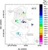 |
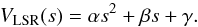
Fig. 1 6.7 GHz CH3OH masers detected over three epochs with the EVN, overlaid on the 1.3 cm continuum imaged with the VLA A-Array. Colored dots show the absolute position of individual maser features, with color denoting the maser VLSR, according to the color-velocity conversion code reported on the right side of the panel4. Maser absolute positions are relative to the epoch 2005 September 9, which is the first of the five VLBA epochs used by Moscadelli et al. (2009) to measure absolute positions and proper motions of the 12 GHz CH3OH masers in NGC 7538 IRS1. Dot size is proportional to the logarithm of the maser intensity. Masers are grouped in different clusters, labeled using capital letters from “A” to “E”. The 1.3 cm map (dotted contours) was produced using archival data, originally reported by Gaume et al. (1995). Plotted contours are 7%, 10% to 90% (in steps of 10%), and 95% of the map peak, 0.022 Jy beam-1. Dotted arrows point to the main 1.3 cm continuum peaks, which are named following the notation by Gaume et al. (1995). The beam of the VLA-A 1.3 cm observations is reported in the insert in the bottom right of the panel. |
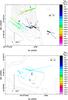 |
Fig. 2 Proper motions of 6.7 GHz CH3OH masers detected over three epochs with the EVN. Symbols, colors and contours have the same meaning as in Fig. 1. The plotted field of view includes the maser clusters “A”, “B”, “C” and “D” (top panel), and cluster “E” (lower panel). Colored arrows show the measured maser proper motions, with dotted arrows denoting the most uncertain measurements. The scale for the proper motion amplitude is given by the black arrow in the lower left corner of each panel. |
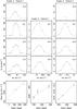 |
Fig. 3 Spectral profiles and time variation in peak velocities of selected maser features of cluster “A”. The plots in each column show a distinct maser feature in the cluster, labeled according to Table 2. (Top panels) Spectral profiles of maser features at different epochs, from Epoch 0 or Epoch 1 down to Epoch 3. The spectra (black dots) are produced by plotting the spot intensity vs. the spot channel velocity. For sufficiently well sampled maser spectra, the dotted curve shows the Gaussian profile fitted to the spectral emission. (Bottom panels) Plot of the maser peak velocity (with the associated errorbar) vs. the observing epoch (expressed in days elapsed from Epoch 0). The dotted line gives the least-square linear fit of velocities vs. time. |
3.1.2. l.o.s. acceleration
For a selection of features in each maser cluster, Figs. 3 to 7 show the Gaussian fit of the maser spectral profiles and the linear fit of the variation in the peak velocity with the observing epoch. These figures show that the spectrum of relatively strong maser features is reasonably well fitted with a Gaussian profile, allowing us to derive the maser peak velocity at a given epoch with a typical accuracy of ~0.01 km s-1, about ten times smaller than the velocity resolution of 0.09 km s-1. Remarkably, these plots show that the peak velocity of many 6.7 GHz features vary linearly with time, providing a measurement of maser l.o.s. accelerations of typical amplitude of ~10-3–10-2 km s-1 yr-1. For each maser cluster, Table 3 reports the values of the measured l.o.s. accelerations for features which are persistent in time, with peak flux densities >3 Jy beam-1, and with a sufficiently well sampled maser spectrum. Figure 8 shows the spatial distribution of maser l.o.s. accelerations inside each cluster. We note that features in cluster “A” have similar values of l.o.s. acceleration around 0.01 km s-1 yr-1, while in clusters “B” and “C” there is a larger scatter, with both positive and negative values from −0.019 to 0.016 km s-1 yr-1. Finally, in cluster “E” most of the measurements are compatible with a null value of maser l.o.s. acceleration (see Table 3). We discuss the implications of these accelerations in terms of gas dynamics in Sect. 5.
Maser feature l.o.s. acceleration.
3.2. Kinematics of NH3 inversion lines
We have mapped the hot NH3 gas from metastable transitions (6,6) up to (13,13) with 0.̋2 resolution towards NGC 7538 IRS1. These transitions are observed in absorption against the strong ultra-compact Hii region and cover upper-state energies, Eup, from 400 K to 1700 K, probing the hottest molecular gas in the region. For each transition, we derived spectral profiles (Fig. 9) and maps of the velocity field (Fig. 10). The full analysis of this dataset, including kinematics and physical condition estimates, will be presented in a separate paper (Goddi et al., in prep.). In this paper, we will focus on the kinematics of the thermal molecular gas as probed by NH3 on scales of 500–1500 AU, to complement the small scale dynamics probed by CH3OH masers.
For each transition, we produced spectra by mapping each spectral channel and summing the flux density in each channel map, separately for the core and the southern component (top and bottom panels of Fig. 9, respectively). Towards the core, multiple transitions show similar line profiles, central velocities (Vc from −58.2 to −59.4 km s-1), and velocity widths (ΔW = 6.8–9.9 km s-1) of the main hyperfine component, as determined from single-Gaussian fits. Despite showing similar values, there are non-negligible changes in ΔW and Vc with (J,K), as compared with the velocity resolution (0.4 km s-1). The central velocity of the optically thick lines, (6,6) and (7,7), gives a good estimate of the systemic velocity, −59.4 km s-1, the same value quoted by Qiu et al. (2011) from several molecular lines with Eup = 16–133 K imaged at 1.3 mm with the SMA. Interestingly, based on CARMA and SMA observations, Zhu et al. (2013) report a similar value for the systemic velocity employing less excited lines at 1.3 mm, but also find an average peak velocity of −58.6 km s-1, using more highly excited (and more optically thin) lines at 0.86 mm. Similarly, we find that the central velocity of the (13,13) line, −58.2 km s-1, is higher than that of the (6,6) line. We also find the largest linewidth (9.9 km s-1) for the (13,13) line.
In Fig. 10, we show the intensity-weighted l.o.s. velocity fields (or first moment maps) for four NH3 transitions, overlaid on the 1.3 cm continuum emission. The positions and VLSR of CH3OH maser features are also overlaid. The NH3 absorption follows closely the continuum emission, as expected. In particular, for lower excitation transitions, (6,6) and (9,9), the absorption is extended N–S across ≈1′′(2700 AU), and reveals two main condensations of hot molecular gas associated with the core and the southern spherical component identified by Gaume et al. (1995) at 1.3 cm (Fig. 1). The highest excitation NH3 lines, (10,10) and (13,13), originate from the core of the radio continuum, and probe the hottest gas associated with clusters “A”, “B”, and “C” of CH3OH masers. The southern spherical component, associated with cluster “E” of CH3OH masers, has the weakest integrated absorption and it is not detected in the highest-JK transitions.
Remarkably, the NH3 absorption towards the core shows a distinct velocity gradient in each line, with redshifted absorption towards NE and slightly blueshifted absorption towards SW with respect to the hot core centre, where the highest values of velocity dispersion are also observed. The velocity gradient is at a PA ≈ 30°–40°, and has a magnitude ΔV ≈ 5 → 9 km s-1, going from the lower-excitation to the higher-excitation lines. A similar PA (≈43°) is measured by Zhu et al. 2013 from SMA images of the OCS(19–18), CH3CN(12–11), and 13CO(2–1) lines with 0.̋7 angular resolution.
Despite a qualitative agreement, there are some significant differences in the velocity field probed by NH3 and CH3OH masers. In Sect. 4.2, we will show that this is a direct consequence of the limited angular resolution of the NH3 maps which do not resolve the northern and southern components of the radio continuum.
4. Ordered kinematical structures
4.1. 6.7 GHz CH3OH masers
Figure 11 evidences an ordered spatial and VLSR distribution of maser features in each of clusters “A”, “B” and “C”. The maser features of cluster “A” show a remarkable positional alignment as well as a regular change in VLSR with position. Figure 11 shows that the majority of the maser features of clusters “B” and “C” is also distributed close to a line with a monotonic variation in the maser VLSR along the major axis of the distribution. A least-square fit to the positions of maser features in clusters “A” and the combined clusters “B” + “C”, gives PA of the major axis of 107°and 71°, respectively. For each group of features, Fig. 12 plots the maser VLSR versus positions projected along the axis of the distribution. We fitted the position-velocity distribution of masers with both a linear and quadratic curve, demonstrating that the change of VLSR with position is better represented by a quadratic curve than a line.
In particular, indicating with s the axis-projected position of a maser feature,
we can write VLSR as a quadratic polynomial of the
variable s:
 (1)The coefficients we
derived from the least-square fit are the following:
(1)The coefficients we
derived from the least-square fit are the following: 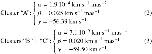 It
is worth noting that while the fitted values of α do not depend on the choice of the
s = 0
position along the major axes of the distributions, β and γ vary, respectively,
linearly and quadratically with the offset in the origin of the coordinate s.
It
is worth noting that while the fitted values of α do not depend on the choice of the
s = 0
position along the major axes of the distributions, β and γ vary, respectively,
linearly and quadratically with the offset in the origin of the coordinate s.
For a physical meaning of these parameters, see Sect. 5.2.
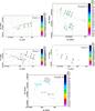 |
Fig. 8 l.o.s. accelerations measured for individual 6.7 GHz maser features. Each panel shows a different cluster, from “A” to “E”. For each maser feature, the value of the l.o.s. acceleration is quoted in km s-1 yr-1. Symbols, colors and contours have the same meaning as in Fig. 1. In panels of the maser clusters “A”, “B” and “C”, the dashed line indicates the major axis of the maser feature’ spatial distribution, and the star marks the reference point to measure axis-projected offsets (see Sect. 4.1). |
 |
Fig. 9 Spectral profiles for NH3 inversion transitions (6,6), (7,7), (9,9), (10,10), and (13,13) observed toward NGC 7538 IRS1 with the JVLA B-Array. The upper panel is showing the spectra integrated over the core component of the 1.3 cm continuum emission (see Fig. 1), and the lower panel the spectra integrated towards the southern spherical component. An offset in flux density was applied to better evidence their spectral profiles. The velocity resolution is 0.4 km s-1 and the l.o.s. velocities are with respect to the local standard of rest (LSR). The dashed green (at −59.4 km s-1) and red (at −58.2 km s-1) lines indicate the central velocity of the least, (6,6), and most, (13,13), excited transitions, respectively, determined by fitting a single Gaussian to the transition spectral profile. In the southern component only the (6,6), (7,7), and (9,9) lines are clearly detected. The upper state energy levels of transitions shown here are ≈408–1693 K. |
4.2. NH3
The velocity field of the hot molecular gas traced by the NH3 inversion lines shows a VLSR gradient at PA (30°–40°), intermediate between the PA of the major axes of the maser clusters “B” + “C” (71°) and “A” (–73°). While towards the clusters “B” + “C”, the absorption occurs at approximately the same VLSR in all NH3 lines (−59 to −61 km s-1), a large change in the absorption velocity (−58 to −52 km s-1), is observed to the E–NE of the cluster “A”, going from the (6,6) to the (13,13) line.
To better compare the NH3 and 6.7 GHz maser VLSR gradients, we extracted a strip from the NH3 first-moment maps along the major axis of the clusters “A” and “B” + “C”, and we plotted in Fig. 13 the NH3 average VLSR vs the axis-projected positional offset. Since the major axis of both maser clusters is oriented close to E–W, the strip value is calculated taking the average velocity of three pixels (0.̋04 in size), the central one along the major axis and the other two to the north and the south of the first pixel, respectively.
Figure 13 reveals two elements. First, there is a clear trend for a steepening of the slopes of the VLSR profiles going from the (6,6) to the (13,13) inversion lines of NH3, for both maser clusters. In fact, the VLSR gradient steadily increases with the excitation of the NH3 inversion transition, from 6 × 10⁻⁴ km s-1 mas-1 (for the (6,6) line) to 6 × 10⁻³ km s-1 mas-1 (for the (13,13) line) in the cluster “A”, and from 4 × 10⁻³ km s-1 mas-1 (for the (6,6) line) to 10-2 km s-1 mas-1 (for the (13,13) line) in the clusters “B” + “C”. This shows that towards both maser clusters, a VLSR gradient is detected also in the NH3 inversion lines. The second element is that the gradients traced in NH3 are significantly shallower than those measured with the 6.7 GHz masers (≈2 × 10⁻² km s-1 mas-1), particularly for cluster “A”. In the rest of this section, we show that this is an effect of the lower angular resolution of the NH3 maps with respect to the VLBI measurements of CH3OH. In particular, the angular resolution of the NH3 JVLA observations (≈0.̋2) is comparable to or higher than both the separation and the size of the maser clusters “A”, “B”, and “C”. Therefore, the NH3 first-moment maps, over regions of weaker signal, could be heavily contaminated by nearby (within the synthesized beam) strong absorption at different VLSR.
To investigate this problem, we determined the VLSR distribution of the NH3 inversion lines in an alternative way, by Gaussian-fitting the position of the compact absorption feature in individual spectral channels with good SNR (≥5σ), and producing plots of channel peak positions, collected in Fig. 14, where also the channel VLSR and the intensity are reported. Figure 14 illustrates three points: 1) the absorption of all the NH3 lines is much stronger towards the clusters “B” + “C” than towards the cluster “A”; 2) the absorption occurs at well separated velocities, at VLSR≲−58 km s-1 towards the clusters “B” + “C” and at VLSR≳−55 km s-1 towards the cluster “A”; 3) for any of the NH3 lines, no channel is found with absorption peaking nearby the linear maser distribution of cluster “A”. Looking at Fig. 10, we stress now two effects: 1) the reddest pixels of the NH3 first-moment maps are found to the NE of the cluster “A”, i.e., at the largest distance from the clusters “B” + “C”; 2) in correspondence of the linear maser distribution of cluster “A”, the intensity-weighted velocities of NH3 are biased to more negative values than the maser VLSR (see also Fig. 13, upper panel). We ascribe the differences between the velocity field shown by the NH3 first-moment maps in Fig. 10 and the channel peak maps in Fig. 14 to the contamination of the stronger absorption at more negative VLSR of the clusters “B” + “C” over the region of the cluster “A” (the two clusters are unresolved in our NH3 maps).
The most remarkable difference between the plots of Fig. 14 and the first-moment maps, is that the (weak) reddest NH3 absorption appears to trace the extension of the linear maser distribution of the cluster “A” to SE, rather than emerging from a region to the NE of the maser line, as shown in the first moment maps.
We will discuss more in detail the relation between the CH3OH maser and NH3 line VLSR distributions in Sect. 6.
5. Edge-on disk model
5.1. Qualitative assessment
In this Section, we present a kinematical model to interpret our observational findings, in particular the regular VLSR patterns described in Sect. 4. Here, we focus on the clusters “A” and “B” + “C”, which share several geometrical and kinematical properties:
-
1)
linear or elongated spatial distribution;
-
2)
regular variation in VLSR with position along the major axis of the distribution;
-
3)
proper motions approximately parallel to the elongation axis;
-
4)
average amplitude of proper motions (≈5 km s-1) similar to the variation in VLSR (4–6 km s-1) across the maser cluster.
For cluster “A”, Pestalozzi et al. (2004) previously proposed a model of edge-on (Keplerian) disk to explain the regular velocity structure identified with the 6.7 and 12.2 GHz masers by Minier et al. (1998). Recently, Pestalozzi et al. (2012) determined the internal proper motions for four intense, 12 GHz CH3OH masers in cluster “A”, finding that they are aligned with the cluster orientation and have amplitudes in the range 1–9 km s-1, in good agreement with our results for six 6.7 GHz masers (see Table 2). The two findings that the maser VLSR increases from NW to SE and all the features move concomitantly to SE (see Fig. 2), constrain all the features of cluster “A” to reside on the near-side of the disk.
We report here for the first time evidence of rotation for clusters “B” + “C”. The distribution of maser positions and proper motions in clusters “B” + “C” is less regular than for the cluster “A”. Several features of the clusters “B” + “C” have positions not closely aligned with the major axis of the cluster (see Fig. 11) and a few proper motions are oriented at a large angle from the cluster axis. Both elements suggest a small deviation from edge-on rotation. Indicating with id the angle between the disk plane and the l.o.s., the components of velocities and accelerations along the l.o.s. would decrease by a factor cos(id) while the components on the plane of the sky transversal to the disk major axis would be proportional to the factor sin(id). Looking at Tables 2 and 3, typical relative errors for the proper motion components and l.o.s. accelerations are of 10–20%, therefore a deviation from the edge-on geometry by less than id ≈ 20°cannot be revealed with our data. In the following, when we use the term “edge-on” referred to the maser clusters “B” + “C”, we mean a deviation by less than ≈20° from an exactly edge-on geometry. Another difference with respect to cluster “A” is that in the clusters “B” + “C” nearby maser features appear to be moving in opposite directions (NE vs. SW; see Fig. 2). We argue however that, considering that the maser VLSR increases from SW to NE, the observed pattern of proper motions in clusters “B” + “C” could still be consistent with rotation (seen about edge-on) if the masers moving to NE and SW were, on the near- and far-side of the rotating structure, respectively.
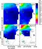 |
Fig. 10 Velocity fields of four inversion transitions of NH3, (6,6), (9,9), (10,10), and (13,13), as measured towards NGC 7538 IRS1 with the JVLA B-Array. In each panel, the positions of the 6.7 GHz CH3OH masers (black-circled, colored dots) are overlaid on the NH3 image. The conversion code between colors and VLSR is indicated in the wedge to the right side of the upper right panel. Dot size is proportional to the logarithm of the maser intensity. Dotted contours have the same meaning as in Fig. 1. In the bottom right panel, the labels of the maser clusters and the names of the main 1.3 cm continuum peaks are given. |
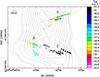 |
Fig. 11 Linear fits to the spatial distributions of maser features in cluster “A”, and in the combined clusters “B” + “C” (dashed lines). Symbols, colors and contours have the same meaning as in Fig. 1. To fit the maser spatial distribution in these clusters, we have selected a subset of features closely aligned along the cluster major axis, excluding the subgroup of weak features scattered to the SE of cluster “A”, the subgroup of features of cluster “B” lying further south, and the subgroup in cluster “C” more detached to NW. The stars labeled IRS1a and IRS1b mark the YSO positions, as discussed in Sect. 6. |
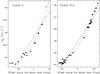 |
Fig. 12 Maser VLSR versus position projected along the major axis of the spatial distribution for the maser cluster(s) “A” (left panel) and “B” + “C” (right panel). The positional offsets are measured with respect to the YSO positions shown in Fig. 11. Maser (relative) positions and VLSR are known with an accuracy better than 1 mas (see Table 2) and 0.1 km s-1 (see Table 1), respectively. These plots are produced considering only the features closely aligned along the cluster major axis. Dot size is proportional to the logarithm of the maser intensity. The linear and quadratic fit to the plotted distribution is indicated with a black dashed and red dot-dashed line, respectively. |
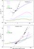 |
Fig. 13 Colored curves show strips of the first-moment map of different NH3 transitions, taken along the major axis of the maser clusters “A” (upper panel) and “B” + “C” (lower panel) . Colored bars along the “Y” axis mark the mean VLSR of the NH3 lines. The association color–NH3 transition is indicated in the upper left corner of the panel. Black dots report the 6.7 GHz masers of the clusters, selecting only the features closely aligned along the cluster major axis. Dot size is proportional to the logarithm of the maser intensity. The linear and quadratic fits to the maser distribution are indicated with a black dashed and black dot-dashed line, respectively. Colored dotted lines show the linear fits to the first-moment strips of the NH3 transitions. |
Figure 8 and Table 3 show that the l.o.s. acceleration for individual masers in cluster “A” is always positive. If we interpret these measurements in terms of centripetal acceleration, a positive value of acceleration is indeed expected if the maser emerges from the near-side of the disk, as indicated by the orientation of the measured proper motions. For the maser clusters “B” + “C”, the situation is more complex, because their l.o.s. acceleration varies from −0.019 km s-1 yr-1 to 0.016 km s-1 yr-1. For centripetal acceleration, we expect the masers rotating on the near- and far-side of the disk to have positive and negative values of l.o.s. acceleration, respectively. The comparison between Tables 2 and 3 shows that this is indeed the case. Accurate (SNR > 3σ) measurements of l.o.s. acceleration are derived for the (intense) features with label numbers from #1 to #5 in cluster “B” and #1, #3 and #5 in cluster “C” (see Table 3). Out of these eight features, proper motions are measured for five (see Table 2). Consistently with our hypothesis, features moving either to NE or SW, i.e., either on the near- or far-side of the disk, have either positive or negative values of l.o.s. acceleration. Therefore, for the small subset of features for which both proper motions and l.o.s. accelerations are well determined, our measurements appear to be qualitatively consistent with a model of rotation.
In an alternative scenario, linear distributions of 6.7 GHz masers with regular l.o.s. velocity gradients could trace collimated outflows, as proposed by De Buizer (2003) and De Buizer et al. (2009) based on H2 near-IR observations and interferometric mapping of the SiO 2–1 line emission in CH3OH maser sources, respectively. In that case, maser proper motions would still be parallel to the maser distribution axis, and the observed maser l.o.s. accelerations could characterize accelerating protostellar outflows. And in fact, this has been shown to be the case in some high-mass YSOs using VLBI measurements of CH3OH masers (e.g., Moscadelli et al. 2011, 2013). We argue however that the observed patterns of maser VLSR proper motions and l.o.s. accelerations in NGC 7538 cannot be explained in terms of a collimated jet neither for the cluster “A” nor for clusters “B” + “C”. In cluster “A”, the maser VLSR increases concertedly with the proper motions, and, if masers are observed in foreground of the continuum emission, that indicates that the masers move and are accelerated towards and not away from the continuum emission, that is the putative location of the exciting protostar. This evidence obviously contrasts with an interpretation in terms of a jet ejected from the protostar. For clusters “B” + “C”, a collimated flow cannot explain neither the opposite orientation of velocity vectors nor the accelerations with both positive and negative sign in nearby maser features. In fact, a collimated jet requires that the gas particles in the same lobe would have velocities with the same orientation and, if the flow is accelerated, similar accelerations. Besides these compelling elements, we measure maser velocities of only 5 km s-1 (on average), which are clearly too low with respect to typical velocities of protostellar jets close to their axis, that are measured to vary from tens to hundreds of kilometer per second using, for example, water masers (e.g., Goddi et al. 2005).
In summary, our measurements of velocity and acceleration towards both clusters “A” and “B” + “C” are qualitatively consistent with edge-on rotation, and inconsistent with expansion in collimated jets. In the rest of this Section, we make a more quantitative analysis presenting a best-fit model to the data.
5.2. Maser distribution on the edge-on disk
If all the 6.7 GHz masers in each cluster rotated at the same radial distance from the
star, one would expect:  (4)where Ω is the (constant) angular velocity, and
s is the
sky-projected distance from the star along the maser elongation axis.
(4)where Ω is the (constant) angular velocity, and
s is the
sky-projected distance from the star along the maser elongation axis.
The simplest explanation for the quadratical (rather than linear) dependence of
VLSR with s (see Fig. 12) is that Ω is not constant but varies (as first approximation)
linearly with s, i.e.:  (5)where
α and
β are the
second and first order coefficients of the quadratic curve fitted to the change of
VLSR with s (see Sect. 4).
(5)where
α and
β are the
second and first order coefficients of the quadratic curve fitted to the change of
VLSR with s (see Sect. 4).
Knowing the maser VLSR and dVLSR/ ds, assuming edge-on rotation and using Eq. (5), we show in the Appendix that it is possible to estimate both the sky-projected position of the centre of rotation (i.e., the star) and the LSR systemic velocity. The stellar positions derived this way for individual maser clusters are indicated with a star symbol in Figs. 8 and 11. We also used the stellar position to calculate the offset along the major-axis of the maser distributions in Fig. 12. Therefore, the fitted quadratic coefficients α, β and γ, introduced in Sect. 4, have the physical meaning of the derivative of Ω with s, the value of Ω at the star position, and the LSR systemic velocity, respectively.
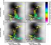 |
Fig. 14 Emission centroids of NH3 fitted as a function of velocity (open squares) and CH3OH masers (filled circles) overlaid on the 1.3 cm continuum map (black image and white contours). Color denotes VLSR (color scale on the right-hand side). The sizes of squares and circles scale linearly and logarithmically with the flux density of NH3 and CH3OH maser emission, respectively. The relative alignment between NH3 and CH3OH is accurate to ~30 mas. Note that NH3 emission distributes between IRS1a and IRS1b, shows a velocity gradients roughly N–S, and is strongest towards IRS1a. |
We notice that the estimates for the stellar positions and LSR velocities from our analysis agree with other independent measurements. In particular, Fig. 11 illustrates that for both clusters “A” and “B” + “C” the derived stellar position falls close to the associated 1.3 cm continuum peak (the northern and southern core, respectively; see Fig. 1), despite the 1.3 cm continuum beam is about ten times bigger than the 6.7 GHz maser beam. The continuum peak could effectively mark the star position if the continuum comes from a hypercompact Hii region. In addition, the model-inferred LSR systemic velocity for the maser clusters “B” + “C”, –59.5 km s-1 (see Sect. 4.1), is in very good agreement with the LSR systemic velocity of the dense clump probed by the lower excitation NH3 lines, –59.4 km s-1 (see Sect. 3.2). If the star exciting the maser clusters “B” + “C” is the most massive in the region (see Sect. 5.3) and the lower excitation NH3 lines probe the molecular core from which the young star is forming, then we expect to observe similar velocities for both the star and the natal core.
For an edge-on disk in centrifugal equilibrium, one can write: 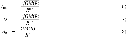 where
G is the
gravitational constant, M(R) is the mass enclosed within
the radius R,
and Vrot and Ac are the
rotational velocity and the centripetal acceleration, respectively.
where
G is the
gravitational constant, M(R) is the mass enclosed within
the radius R,
and Vrot and Ac are the
rotational velocity and the centripetal acceleration, respectively.
We can express the dependence of the disk mass with radius in terms of a power-law:
 (9)We do not expect
the gas density to increase with radius (from the star), so we can exclude values of
q>
3. The value q = 0 describes the Keplerian case, while the value
q = 2
corresponds to a flat disk with constant density.
(9)We do not expect
the gas density to increase with radius (from the star), so we can exclude values of
q>
3. The value q = 0 describes the Keplerian case, while the value
q = 2
corresponds to a flat disk with constant density.
Employing Eq. (9), we can rewrite Eqs.
(6) to (8) as:  Finally,
indicating with R0 the maser radius along the l.o.s. to
the star (i.e., at s =
0), and combining Eqs. (5) and (11), one can express
R in terms
of s:
Finally,
indicating with R0 the maser radius along the l.o.s. to
the star (i.e., at s =
0), and combining Eqs. (5) and (11), one can express
R in terms
of s:
 Equation
(14) sets the maser positions onto the
near or far-side of the rotating, edge-on disk. A comparison between the orientation of
the VLSR gradient and the proper motions
suggests that all (most of) the maser features of the cluster “A” (“B” + “C”) reside on
the near-side of the disk (see Sect. 5.1). Figure
15 illustrates the maser distribution patterns on
the disk for a range of plausible values of R0 and q.
Equation
(14) sets the maser positions onto the
near or far-side of the rotating, edge-on disk. A comparison between the orientation of
the VLSR gradient and the proper motions
suggests that all (most of) the maser features of the cluster “A” (“B” + “C”) reside on
the near-side of the disk (see Sect. 5.1). Figure
15 illustrates the maser distribution patterns on
the disk for a range of plausible values of R0 and q.
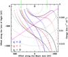 |
Fig. 15 The colored curves are the loci of the 6.7 GHz features, as derived from the edge-on disk model described in Sect. 5.2. We assume that the masers emerge from the near-side of the disk. Maser positions are described by the Eq. (14) (see Sect. 5), using the coefficients α = 7.1 10-5 km s-1 mas-2 and β = 0.020 km s-1 mas-1, derived in Sect. 4.1 fitting the change in maser VLSR with position in the clusters “B” + “C”. The colors black, red and blue identify the maser patterns corresponding to the values of the exponent q equal to 0, 1, and 2, respectively. Light squares, heavy solid line and light triangles are used to plot the curves corresponding to the values of the maser radius at the star position, R0 = 250, 500 and 750 AU, respectively. The star marks the location of the star at the disk centre. The magenta solid line indicates the linear change of the maser angular velocity Ω with the position projected along the cluster major axis. The two green bars mark the range of major-axis projected offset over which the 6.7 GHz masers of the clusters “B” + “C” distribute. Dashed arcs indicate circular orbits at steps of 200 AU in radial distance. |
 |
Fig. 16 Result of the model-fit for the cluster “A” (upper panel) and clusters “B” + “C” (lower panel). The colored map shows the distribution of χ2 (calculated using Eq. (20)) around the best-fit position, plotting values from the minimum of χ2 up to 50% above the minimum. The color-value conversion code is shown by the wedge on the right of the panel. The white cross shows the position of the minimum of χ2. The full white contours show levels of 10%, 20%, 30% and 40% above the minimum value of χ2. |
5.3. Fit of the model parameters
In Sect. 5.2 we have proposed an interpretation for the observed regular variation in the maser VLSR with sky-projected position based on the assumption that the maser emission emerges from an edge-on disk in centrifugal equilibrium. We have shown that the regular pattern in VLSR can be reproduced if masers distribute on the edge-on disk along specific curves described by the two parameters R0 and q. Now, we can use our measurements of maser l.o.s. accelerations and proper motions to constrain the model of edge-on rotation and derive the best values of R0 and q for each of the two maser clusters “A” and “B” + “C”.
Denoting with ![\begin{eqnarray} \label{z} z &=& \sqrt{R^2-s^2} \\[3mm] \label{M0} M_0 &=& \beta^2 R_0^3 / G \\[3mm] \label{A0} A_0 &=& G M_0 / R_0^2 \end{eqnarray}](/articles/aa/full_html/2014/06/aa23420-14/aa23420-14-eq104.png) the
position along the l.o.s., the mass within the radius R0, and the
acceleration at R0 (with G indicating the
Gravitational Constant), respectively, the sky-projected velocity, Vs, and the
l.o.s. acceleration, Az, at the location
identified by the spatial coordinates R and z is given by:
the
position along the l.o.s., the mass within the radius R0, and the
acceleration at R0 (with G indicating the
Gravitational Constant), respectively, the sky-projected velocity, Vs, and the
l.o.s. acceleration, Az, at the location
identified by the spatial coordinates R and z is given by:  Before
describing the procedure adopted to fit maser velocities and accelerations, we verify the
consistency of our model of centrifugally supported edge-on rotation for the case of the
maser cluster “A”. Equations (7) and (8) imply R =
Ac/ Ω2, which
at R =
R0, following our definitions (see Eqs.
(13), (17) and (19)), can be
rewritten as R0 =
A0/β2.
β = 0.025
km s-1
mas-1for the
cluster “A” (see Sect. 4.1). Since, over the cluster
“A”, the measured l.o.s. accelerations are all in the range 0.01 ± 0.001 km s-1 yr-1 (see Fig. 3 and Table 3), we can
confidently take A0
= 0.01 km s-1 yr-1. Thus, we find R0 ≈ 570 AU (215
mas at the distance of NGC 7538 IRS1) and from the product of R0 and
β a
rotational velocity of 5.4 km s-1. That compares well with the average maser velocity
projected along the major axis of the cluster “A”, which is 5.1 km s-1. Such a remarkable agreement
between the value of rotational velocity derived from the maser VLSR and l.o.s.
accelerations, in the framework of the model of edge-on rotation, and the direct
measurement of maser proper motions, makes us confident that the adopted model is able to
correctly reproduce the maser kinematics.
Before
describing the procedure adopted to fit maser velocities and accelerations, we verify the
consistency of our model of centrifugally supported edge-on rotation for the case of the
maser cluster “A”. Equations (7) and (8) imply R =
Ac/ Ω2, which
at R =
R0, following our definitions (see Eqs.
(13), (17) and (19)), can be
rewritten as R0 =
A0/β2.
β = 0.025
km s-1
mas-1for the
cluster “A” (see Sect. 4.1). Since, over the cluster
“A”, the measured l.o.s. accelerations are all in the range 0.01 ± 0.001 km s-1 yr-1 (see Fig. 3 and Table 3), we can
confidently take A0
= 0.01 km s-1 yr-1. Thus, we find R0 ≈ 570 AU (215
mas at the distance of NGC 7538 IRS1) and from the product of R0 and
β a
rotational velocity of 5.4 km s-1. That compares well with the average maser velocity
projected along the major axis of the cluster “A”, which is 5.1 km s-1. Such a remarkable agreement
between the value of rotational velocity derived from the maser VLSR and l.o.s.
accelerations, in the framework of the model of edge-on rotation, and the direct
measurement of maser proper motions, makes us confident that the adopted model is able to
correctly reproduce the maser kinematics.
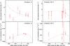 |
Fig. 17 Comparison of the measurements and best-fit values for the cluster “A” (left panels) and clusters “B” + “C” (right panels). Upper and lower panels refer to the velocities (projected along the cluster major-axis) and the l.o.s. accelerations, respectively. Red crosses and errorbars give the measurements and corresponding errors, plotted vs. the maser position. The black dashed line shows the change of the model-predicted quantities along the maser pattern, with black crosses denoting the values in correspondence of the maser positions. |
The best values for R0 and q are derived by minimizing
the χ2 expression: 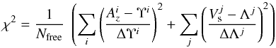 (20)where
Υ (ΔΥ) and Λ (ΔΛ) denote the amplitudes (and corresponding
errors), of the measured l.o.s. accelerations and velocity components
along the major axis of the maser cluster, respectively, and the index i and j run over the features of
the cluster with measured acceleration and proper motion, respectively (see Tables 2 and 3).
Nfree is the degree of freedom of the
model, defined by the difference between the number of measurements and the number (2) of
free parameters. For the cluster “A”, the χ2 is calculated using all the measured
accelerations and proper motions (i.e., i = 5 and j = 6). For the clusters
“B” + “C”’, beside excluding the subset of features more detached from the major axis of
the maser distribution (see Figs. 12 and 8), we did not consider the features #7 and #17 of
cluster “C”, whose proper motions are directed at large angle from the cluster axis (see
Fig. 2), and feature #1 of cluster “B”, whose l.o.s.
acceleration deviates very much (by 15σ) from the average value of nearby features (with
this selection, we have i =
5 and j =
8). The errors of the l.o.s. accelerations, ΔΥ, are those reported in Table 3. For the proper motions, besides the formal errors
derived from the least-square fit of position offsets with time (reported in Table 2), we also need to consider a systematic error on the choice
of the reference system, the “centre of Motion” (see Sect. 3.1.1), which could not represent adequately the star/disk system. We have shown
above that, at least for the masers of the cluster “A”, the sky-projected velocity
inferred from the model (using the maser VLSR and l.o.s. accelerations) agrees
with the average amplitude of measured proper motions within a few tenths of kilometer per
seconds. Therefore we can conservatively estimate the systematic error on the proper
motions to be ≲1 km
s-1. To perform
the model-fit, the uncertainties on the velocity, ΔΛ, are calculated by adding in quadrature
to the measurement errors (read from Table 2) a systematic
error plateau of 1 km s-1.
(20)where
Υ (ΔΥ) and Λ (ΔΛ) denote the amplitudes (and corresponding
errors), of the measured l.o.s. accelerations and velocity components
along the major axis of the maser cluster, respectively, and the index i and j run over the features of
the cluster with measured acceleration and proper motion, respectively (see Tables 2 and 3).
Nfree is the degree of freedom of the
model, defined by the difference between the number of measurements and the number (2) of
free parameters. For the cluster “A”, the χ2 is calculated using all the measured
accelerations and proper motions (i.e., i = 5 and j = 6). For the clusters
“B” + “C”’, beside excluding the subset of features more detached from the major axis of
the maser distribution (see Figs. 12 and 8), we did not consider the features #7 and #17 of
cluster “C”, whose proper motions are directed at large angle from the cluster axis (see
Fig. 2), and feature #1 of cluster “B”, whose l.o.s.
acceleration deviates very much (by 15σ) from the average value of nearby features (with
this selection, we have i =
5 and j =
8). The errors of the l.o.s. accelerations, ΔΥ, are those reported in Table 3. For the proper motions, besides the formal errors
derived from the least-square fit of position offsets with time (reported in Table 2), we also need to consider a systematic error on the choice
of the reference system, the “centre of Motion” (see Sect. 3.1.1), which could not represent adequately the star/disk system. We have shown
above that, at least for the masers of the cluster “A”, the sky-projected velocity
inferred from the model (using the maser VLSR and l.o.s. accelerations) agrees
with the average amplitude of measured proper motions within a few tenths of kilometer per
seconds. Therefore we can conservatively estimate the systematic error on the proper
motions to be ≲1 km
s-1. To perform
the model-fit, the uncertainties on the velocity, ΔΛ, are calculated by adding in quadrature
to the measurement errors (read from Table 2) a systematic
error plateau of 1 km s-1.
We have searched for the minimum of χ2 over the parameter space
100 ≤ R0 ≤
1100 AU and 0 ≤
q ≤ 3, in steps of 20 AU for R0 and 0.1 for
q. For the
cluster “A” only, we have optimized the search using a narrower parameter window with
steps of 5 AU for R0 and 0.02 for q. The derived best-fit
values are: 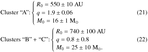 The
quoted uncertainties are formal fit errors evaluated taking the displacement from the
parameter best-value in correspondence of which the χ2 increases by
≈10% above the minimum.
Figure 16 shows the distribution of χ2 around the
position of minimum for the model-fit of both maser clusters.
The
quoted uncertainties are formal fit errors evaluated taking the displacement from the
parameter best-value in correspondence of which the χ2 increases by
≈10% above the minimum.
Figure 16 shows the distribution of χ2 around the
position of minimum for the model-fit of both maser clusters.
Figure 17 presents the comparison between the measured and the best-fit accelerations and velocities. Finally, Fig. 18 shows the modeled positions for maser features of cluster(s) “A” and “B” + “C” on the near-side of the edge-on disk.
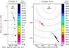 |
Fig. 18 Locations of maser features as derived from the edge-on disk model described in Sect. 5.2, assuming that the masers emerge from the near-side of the disk. Colored dots give the position for features of cluster(s) “A” (left panel) and “B” + “C” (right panel). For each cluster, only the maser features closely aligned along the cluster major axis are considered. Symbols and colors have the same meaning as in Fig. 1. The labeled star marks the YSO position at the disk centre. Dashed arcs indicate circular orbits at steps in radial distance of 500 and 200 AU, for the plot of cluster(s) “A” and ”B” + “C”, respectively. |
6. Nature of the YSOs exciting the 6.7 GHz masers
We propose that the three radio continuum peaks, associated with clusters “A”, “B” + “C”, and “E” of 6.7 GHz CH3OH masers, could mark the position of three distinct YSOs in the region, responsible for the maser excitation. Hereafter, we refer to these YSOs with the names IRS1b, IRS1a, and IRS1c. In the following, we describe their physical properties, based on our CH3OH and NH3 measurements as well as the edge-on disk model presented in Sect. 5.
6.1. IRS1a: the high-mass YSO associated with the maser clusters “B” + “C”
Figure 14 reveals that the strongest absorption in all the NH3 lines occurs at the centre of the maser clusters “B” + “C”, indicating that dense and warm molecular gas is associated with this cluster. Towards the same position, Beuther et al. (2013) detected emission from warm dust and typical hot-core tracers using the PdBI. In particular, the 843 μm dust emission peaks just in correspondence of the maser cluster “B” (Beuther et al. 2013, see their Fig. 1), where the map brightness temperature reaches 219 K. Towards the dust continuum peak, they derive a maximum value of nH2 density of 109 cm-3. Observing NGC 7538 IRS1 with the SMA, Zhu et al. (2013) and Qiu et al. (2011) detected molecular lines from several dense gas tracers (e.g., CH3CN and CH3OH) and derived gas temperatures of ≈250 K. Therefore, we conclude that the 6.7 GHz masers of the clusters “B” + “C” are associated with an hot-core excited by a massive YSO, that we call IRS1a, which is surrounded by a rotating disk.
In the edge-on disk model proposed in Sect. 5.3 for the clusters “B” + “C”, we only poorly constrain the value of the parameter q = 0.8 ± 0.8, but this would be consistent with a Keplerian rotation if q is actually close to zero. Then, most of the ≈25 M⊙ predicted within a radius of ≈740 AU would actually constitute the mass of the high-mass YSO at the disk centre. A YSO of ≈25 M⊙ could account for most of the far-IR luminosity of NGC 7538 IRS1, ~105L⊙ (see, e.g., Davies et al. 2011).
The quasi-Keplerianity of the disk around IRS1a is also supported by the properties of the thermal emission from warm dust and hot gas probed by highly excited molecular lines. For example, the peak value of the 843 μm emission imaged by Beuther et al. (2013), converts to a gas mass contribution over the ~0.̋2 beam (≈500 AU) of only ~1 M⊙, much lower than the total mass of 25 M⊙. More compelling, in multi-transition studies of hot-cores it has been demonstrated that molecular lines of higher excitation emerge from warmer gas at smaller radii from the YSO (see for ex. the study of CH3CN transitions in IRAS 20126+4104 by Cesaroni et al. 1999). The same result seems to hold also for the highly excited NH3 lines in NGC 7538 IRS1 (Goddi et al. in prep.). In this context, the steepening of the slope (from 4 × 10⁻³ km s-1 mas-1 to 10-2 km s-1 mas-1) of the position–velocity plots with the excitation energy of the NH3 line (Fig. 13, lower panel) is consistent with (quasi-)Keplerian rotation, where the angular velocity is expected to increase at smaller radii from the central mass. Unfortunately, the angular resolution of the NH3 observations does not permit a more quantitative analysis on the relation between VLSR gradients and sizes of the emitting regions. As a matter of fact, the measured VLSR gradients are likely only lower limits and no reliable estimate of the size of the absorption region for individual NH3 lines is possible.
Since IRS1a is the dominant YSO in the region and it is surrounded by a rotating disk, we could ask the question if this YSO is responsible for driving some of the outflows identified in the region. It is evident that the direction perpendicular to the disk plane (PA = −19°, the expected outflow direction) is significantly misaligned from the axes of the bipolar CO outflow (PA ≈ − 50°, eyeball value) and the inner core (≲0.′′5) of the radio continuum imaged with the VLA A-array (Fig. 1), oriented mainly N-S (PA ~0°). It is however consistent with the observed NIR fan-shaped region around IRS1 probed by H2 emission (PA ~ −20°; see Fig. 3 by Kraus et al. 2006) and the bending of the outer core of the radio continuum (0.′′5–1′′) towards the West at PA ~−25° (e.g., Campbell 1984; Sandell et al. 2009).
6.2. IRS1b: the YSO associated with the maser cluster “A”
Comparing with the maser clusters “B” + “C”, the cluster “A” presents a more regular
distribution of maser 3-D velocities and l.o.s. accelerations, which in turns allows a
more accurate determination of the parameters of the edge-on disk model (see Sect. 5.3). The value of q = 1.9 derived for the
cluster “A” implies M(R) ∝
R1.9, i.e., the mass within a given radius
increases approximately with the square of the radius. Clearly that can be verified
only if the disk mass dominates the YSO mass. Since the model
determines that a mass M0 = 16M⊙ is contained
within a radius R0
= 550 AU, the mass of IRS1b can be at most of a few M⊙. Assuming an
open disk geometry with the disk height H(R) = 2 tan(α)
R (α denoting the semi-opening angle of the disk), the
molecular (number) density at radius R is: ![\begin{equation} \label{nh2_a} n_{\rm H_2} \approx 2.5 \times 10^{9} \; \frac{1}{\tan(\alpha)} \; \left[\frac{R_0}{R}\right]^{1.1} \; \; {\rm cm}^{-3}. \end{equation}](/articles/aa/full_html/2014/06/aa23420-14/aa23420-14-eq145.png) (23)The spatial
distribution and VLSR of the weak, most redshifted
NH3 absorption in
Fig. 14 is consistent with the edge-on disk model
based on the 6.7 GHz CH3OH masers. The peaks of the most redshifted
NH3 absorption
distribute close to the SE extension of the major axis of the cluster “A” maser disk.
Their projected separations from the estimated position of the YSO IRS1b fall in the range
0.̋1–0.̋15, and their VLSR vary over the interval
[−53, −48] km s-1. Using the quadratic
polynomial fitted to the change of maser VLSR with the projected separation,
s, from the
star (see Sect. 4.1 and Eq. (2)), one would expect a VLSR variation in the interval
[−52, −48.4] km s-1 for s varying across
0.̋1–0.̋15. The good match with the observed range of VLSR for the
reddest NH3
absorption features suggests that NH3 and 6.7 GHz masers trace the same kinematical
structure. The relatively coarse, positional accuracy (≳30 mas) of the weak, reddest
NH3 peaks
prevents a more accurate comparison with the edge-on disk model.
(23)The spatial
distribution and VLSR of the weak, most redshifted
NH3 absorption in
Fig. 14 is consistent with the edge-on disk model
based on the 6.7 GHz CH3OH masers. The peaks of the most redshifted
NH3 absorption
distribute close to the SE extension of the major axis of the cluster “A” maser disk.
Their projected separations from the estimated position of the YSO IRS1b fall in the range
0.̋1–0.̋15, and their VLSR vary over the interval
[−53, −48] km s-1. Using the quadratic
polynomial fitted to the change of maser VLSR with the projected separation,
s, from the
star (see Sect. 4.1 and Eq. (2)), one would expect a VLSR variation in the interval
[−52, −48.4] km s-1 for s varying across
0.̋1–0.̋15. The good match with the observed range of VLSR for the
reddest NH3
absorption features suggests that NH3 and 6.7 GHz masers trace the same kinematical
structure. The relatively coarse, positional accuracy (≳30 mas) of the weak, reddest
NH3 peaks
prevents a more accurate comparison with the edge-on disk model.
Although we detect NH3 absorption only from the most redshifted SE end of the disk, we cannot exclude that absorption may originate from the whole disk structure, including the blueshifted NW end. However, since the angular resolution of the NH3 observations does not allow resolving the disk around IRS1b as well as IRS1a from IRS1b, we expect the NH3 absorption at more negative VLSR to be dominated by the hot-core excited by the high-mass YSO IRS1a, hiding any potential contribution from IRS1b.
Since the brightness of the radio continuum towards the cluster “A” and “B” + “C” is comparable, the relative weakness (by a factor of ≈10) of the NH3 absorption (see Fig. 14) suggests that towards the cluster “A” either the NH3 column density is scarce or there are less favourable excitation conditions. Equation (23) indicates that the gas density traced by the masers in the cluster “A” is comparable or even higher (if the disk is thin) than that in the clusters “B” + “C”. The weakness of the NH3 absorption lines can then be explained with a difference in temperature between IRS1a and IRS1b. This hypothesis is also supported by the properties of the mm dust continuum. Examining the 843 μm map of dust emission of Beuther et al. (2013, see Fig. 1), we see that at the position of the maser cluster “A” (crossed by the 5σ contour level) the map intensity is about one third of the peak value, in the direction of the maser cluster “B”. If the gas density is comparable between the two clusters, the decrease of intensity from dust emission could reflect a lowering in temperature from cluster “B” to cluster “A”. Therefore, we argue that the gas around IRS1b should be at lower temperature than towards IRS1a (i.e. T < 250 K). Coupled with the results of the edge-on disk model, we also expect that the YSO IRS1b is not so massive to significantly ionize (and heat up) the surrounding gas.
Since IRS1b is also a YSO surrounded by a rotating disk, we could ask a similar question as done for IRS1a if also this YSO is responsible for driving any of the outflows identified in the region. The PdBI observations of the HCO+(4–3) line (beam FWHM ≈ 0.̋2) by Beuther et al. (2013, see their Fig. 2, right panel), reveal a collimated bipolar outflow, whose axis is oriented NE–SW and intersects the dust emission a few tenths of arcsec to the NE of the 843 μm continuum peak (aligned with the maser cluster “B”). These two findings are consistent with an outflow driven by IRS1b and collimated by its rotating disk. We also argue that the observed velocity distribution and collimation degree indicate that the outflow lies on the plane of the sky. Beuther et al. (2013) noticed that the HCO+ spectrum extracted towards the direction of the blue-shifted (red-shifted) lobe contained also weak red-shifted (blue-shifted) emission, and suggested that the outflow should be oriented close the l.o.s. However, the detection of both blue- and red-shifted emission from a single outflow lobe can occur also in the case that the outflow axis is close to the plane of sky, if the flow has a significant aperture angle (see for ex. the well-studied case of IRAS 20126+4104 imaged in the HCO+ 1–0 line; see, e.g., Cesaroni et al. 1999). Considered also the high degree of collimation, we think it is more likely that the outflow is oriented close to the plane of the sky rather than along the l.o.s.
We conclude that IRS1a is surrounded by an edge-on disk and drives an outflow on the plane of the sky.
6.3. IRS1c: the YSO associated with the maser cluster “E”
Comparing with the other CH3OH maser clusters, cluster “E” presents a more scattered, quasi-spherical distribution of masers (see Fig. 1). The overall pattern of proper motions is also quite scattered (Fig. 2, bottom panel), with a hint at an average motion of the whole cluster (with respect to the clusters “A” and “B” + “C”) towards East. The internal motions of the masers of cluster “E” are of a few kilometer per seconds both along the l.o.s. and across the sky plane. The feature l.o.s. accelerations are all zero within the measurement errors (see Table 3). Towards this cluster, NH3 lines of different excitation, from the (6,6) to the (9,9) line (see Fig. 10), show absorption at similar VLSR ≈ −60 km s-1(close to the systemic velocity of −59.4 km s-1), indicating that layers of molecular gas with different temperatures and densities (and likely distances from the ionized gas), have no significant relative motions (at least, along the l.o.s.). The NH3VLSR is slightly more negative than that of the 6.7 GHz masers (−58.5 km s-1). We conclude that the circumstellar gas associated with IRS1c is less structured and more quiescent than that in the other YSOs in the region.
Again, the highly excited thermal lines help us estimating qualitatively the physical conditions of the molecular gas around IRS1c. Towards the cluster “E”, the NH3 inversion lines of highest excitation (the (10,10) and (13,13) lines) are not observed in absorption (see Fig. 10). A possible explanation is that the gas temperature is not high enough to excite the population levels of the highest excitation NH3 transitions, suggesting that the temperature in IRS1c may be lower than that of IRS1b, where absorption, although weak, is detected in all the NH3 lines. Accordingly, the 843 μm map of Beuther et al. (2013, see their Fig. 1) shows only a weak (≤3σ) level of dust emission in correspondence of the southern maser cluster “E”, which again points out to lower temperatures (and densities) than towards the cluster “B”, where the dust emission peaks. The presence of a (weak) radio continuum peak (see Fig. 1) suggests that the YSO IRS1c associated with the cluster “E” may also be a massive YSO, if the free-free emission is coming from photoionized gas. If this is the case, IRS1c is likely less massive than the dominant object in the region, IRS1a. If the 6.7 GHz masers of cluster “E” traced molecular gas at the edge of a slow expanding, ultra-compact Hii region, that could account for both the sparse spatial distribution and the slow and scattered proper motions of the masers. Assuming that the expansion velocity increases with the radius, the NH3 absorption could trace less dense gas at greater radii than the 6.7 GHz masers, which could explain why the VLSR of the NH3 lines is more negative (more blueshifted) than that of the masers.
The depicted scenario for the maser cluster “E” is clearly very speculative, and more sensitive, high angular resolution data are needed to put it on a firm observational ground.
7. Discussion
7.1. General implications of the model for NGC 7538 IRS1
In previous section, we described the main properties of the individual YSOs and their surrounding disks, as derived from our CH3OH and NH3 measurements as well as our edge-on disk model. We discuss here general implications of this model.
We start discussing the structure, geometry, and velocity field of the circumstellar gas associated with individual YSOs with respect to the natal molecular clump. Looking at Fig. 14, three regions at different VLSR can be identified in the NH3 absorption: 1) the most redshifted (weak) absorption to the SE of the maser elongation of cluster “A”; 2) the (strong) absorption near the systemic velocity (−59.4 km s-1) towards the centre of the maser clusters “B” + “C”; 3) absorption in between the two maser clusters or YSOs IRS1a and IRS1b, where the gas VLSR steadily increases, going from the centre of the clusters “B” + “C” towards the cluster “A”. One should distinguish here between gas motion between the two YSOs and around a given YSO. Owing to limited angular resolution, close to the cluster “A” the two contributions to the gas motion are not resolved and the direction of the VLSR gradient bends from close to N–S (as it is at the middle point between the two clusters) to NE–SW. Blending of the two different motions accounts also for the orientation of the VLSR gradient visible in the NH3 first-moment maps (see Fig. 10), which is directed NE–SW at PA = 30°–40°. Taking into account the bias introduced by the blending of the two motions, Fig. 14 then indicates that the VLSR gradient in the gas between the two YSOs IRS1a and IRS1b is directed close to N–S and extends from ≈−59 km s-1(at the centre of the clusters “B” + “C”) to ≈−56 km s-1(close to the cluster “A”). This finding suggests that the observed VLSR gradient between the two maser clusters could reflect original gas motions inside the molecular core out of which the YSOs IRS1a and IRS1b have formed.
Since we model the maser clusters “A” and “B” + “C” as two disks close to edge-on, separated by less than 500 AU, we could ask what are the chances of observing two nearby edge-on disks oriented at different PA in the plane of the sky. A possible explanation could be maser excitation effects. In fact, an edge-on geometry implies high column densities of masing molecules, which in turn enable strong amplification of the maser emission. In principle, there could be many YSOs in the region but only those with edge-on disks would be traced by the methanol masers. In practice, we think that this is not the case. In fact, the small separation between IRS1a and IRS1b (i.e., <500 AU) would imply a Jeans length for the collapsing and fragmenting core of at most a few hundreds of AU. Even assuming an average density as high as nH2 = 109 cm-3 (i.e., the peak value measured towards IRS1a by Beuther et al. 2013), the mass of individual fragments would correspond to only a few hundredths of solar mass. We conclude therefore that the presence of other undetected massive YSOs in the region, besides the ones identified by the methanol maser clusters, is unrealistic. An alternative and more plausible explanation could be a physical mechanism producing an edge-on alignment. Surcis et al. (2011) measured the linear polarized emission of all CH3OH masers in the region, finding that the magnetic field is aligned close (within 20°) to the plane of the sky and tend to be oriented perpendicularly to the elongation axes of clusters “A”, “B”, and “C”, that is perpendicular to the disks around IRS1a and IRS1b (see their Table 3). This finding agrees with predictions of star formation models which include magnetic fields (e.g., Banerjee & Pudritz 2007; Seifried et al. 2011). In these models, the collapsing core flattens preferably along a direction perpendicular to that of the magnetic field lines. These predictions are consistent with the general result of a polarimetric survey of CH3OH masers towards high-mass star forming regions (Surcis et al. 2013) and suggest that the magnetic field may be important in regulating the dynamics of the mass-accretion and mass-loss in high-mass YSOs. In this framework, an edge-on geometry for protostellar disks could be favoured if the magnetic field in the natal core (before collapse) was oriented near the plane of the sky. Although this qualitative argument explains the edge-on geometry of the two disks around IRS1a and IRS1b, it does not explain their different PA in the sky.
One could now ask whether the disks around IRS1a and IRS1b are stable or transient
structures. The Toomre stability parameter for disks, Q, is given by the
expression  , with
Ω the angular velocity,
Σ the surface density, and
ΔV the FWHM
linewidth. For the maser cluster “A”, the disk model requires that at R = R0 =
550 AU, Ω =
β = 0.025 km s-1 mas-1, with the disk/envelope mass
equal to M0 =
16M⊙ (see Eq. (21)). Using these parameters, we derive
, with
Ω the angular velocity,
Σ the surface density, and
ΔV the FWHM
linewidth. For the maser cluster “A”, the disk model requires that at R = R0 =
550 AU, Ω =
β = 0.025 km s-1 mas-1, with the disk/envelope mass
equal to M0 =
16M⊙ (see Eq. (21)). Using these parameters, we derive ![\hbox{$Q_{\rm clA} = 0.18 \, \left[\frac{\Delta V}{{\rm km \, s}^{-1}}\right] $}](/articles/aa/full_html/2014/06/aa23420-14/aa23420-14-eq157.png) .
The condition for instability, QclA ≤ 1, is then
satisfied if ΔV ≤
5.6 km s-1. From our NH3 lines, we measure FWHM linewidths of 7–10 km
s-1, where,
however, the two YSOs IRS1a and IRS1b, with a velocity separation of 3 km s-1 (see Sect. 5), are blended together. We then expect QclA ≤
1, that is the massive disk/envelope around IRS1b is probably not
gravitationally stable and could break up into fragments. For IRS1a, if a high fraction of
the 25 M⊙ inside a radius R0 = 740 AU (see
Eq. (22)) actually constitutes the YSO mass, then the disk surface
density should be about one order of magnitude lower than for the disk/envelope around
IRS1b. Since the value of Ω =
0.02 km s-1 mas-1 is comparable, the condition for instability for IRS1a
would require ΔV ≤
1 km s-1. The measured values of FWHM linewidths are definitively
greater than this threshold, indicating that the disk surrounding the high-mass YSO IRS1a
is actually gravitationally stable.
.
The condition for instability, QclA ≤ 1, is then
satisfied if ΔV ≤
5.6 km s-1. From our NH3 lines, we measure FWHM linewidths of 7–10 km
s-1, where,
however, the two YSOs IRS1a and IRS1b, with a velocity separation of 3 km s-1 (see Sect. 5), are blended together. We then expect QclA ≤
1, that is the massive disk/envelope around IRS1b is probably not
gravitationally stable and could break up into fragments. For IRS1a, if a high fraction of
the 25 M⊙ inside a radius R0 = 740 AU (see
Eq. (22)) actually constitutes the YSO mass, then the disk surface
density should be about one order of magnitude lower than for the disk/envelope around
IRS1b. Since the value of Ω =
0.02 km s-1 mas-1 is comparable, the condition for instability for IRS1a
would require ΔV ≤
1 km s-1. The measured values of FWHM linewidths are definitively
greater than this threshold, indicating that the disk surrounding the high-mass YSO IRS1a
is actually gravitationally stable.
In the rest of this section, we will discuss excitation effects and implications on the physical structure of the observed disks. Excitation models predict that the 6.7 GHz CH3OH masers, radiatively pumped by IR radiation, are strongly inverted over an extended range of gas density, 104 cm-3 ≤ nH2 ≤ 109 cm-3, and kinetic temperature, 25 K ≤ TK ≤ 250 K (Cragg et al. 2005). The IR radiation can be produced by warm dust nearby the methanol masing molecules, with an allowed range of dust temperature for efficient maser pumping 100 K ≤ Td ≤ 300 K. Following the discussion in Sect. 6, the gas temperature towards the 6.7 GHz maser clusters in NGC 7538 IRS1 should vary from the lowest value in IRS1c to the highest value (250 K) in IRS1a. Therefore, the gas temperature measured and/or expected towards each maser cluster is within the range predicted by the model of Cragg et al. (2005) for strong maser action. The value of gas density nH2 ~ 109 cm-3 towards IRS1a derived from the SMA observations by Beuther et al. (2013), is close to the upper end of the maser excitation range, but still consistent with the models of Cragg et al. (2005).
A more quantitative comparison between the physical conditions deduced from our kinematical model and those required for maser excitation can be done for IRS1b and the cluster “A”. Looking at the spatial distribution of the maser features onto the edge-on disk (see Fig. 18, left panel), one can see that the maser emission abruptly decreases in intensity and vanishes at radii between 500 and 300 AU. As indicated by Eq. (23), at radii smaller than R0 = 550 AU the local gas density rapidly increases to values nH2 > 109 cm-3, and the masers are probably thermally quenched, in line with the model predictions of Cragg et al. (2005). The edge-on disk model for cluster “A” predicts a maximum radius of 6.7 GHz maser emission of ≈2500 AU, which can also be explained in terms of the maser excitation model of Cragg et al. (2005) if the IR radiation flux at this radius falls below the threshold for efficient maser pumping. Assuming that the dust absorbs the stellar photons and re-emits them at IR wavelengths like a black-body, one derives an inverse square-root dependence for the dust temperature on the distance from the star. If Td ≈ 300 K (i.e., the maximum value expected for efficient pumping) at the smallest maser radii of ≈300 AU, at the largest maser radius of ≈2500 AU Td ≈ 100 K, that is the value indicated by Cragg et al. (2005) as the lower limit for efficient excitation of the 6.7 GHz masers.
From Eq. (23) it is also clear that the opening angle α of the disk around IRS1b has to be large enough (α ≈ 45°) to ensure that the gas density does not exceed the threshold for the thermal quenching even at R ≥ R0. Such a geometry reminds the profiles of the rotationally flattened, circumstellar envelopes observed towards low-mass YSOs at millimeter wavelengths (Koerner & Sargent 1995) and in the near-IR (Cotera et al. 2001). If high-mass star formation proceeds as a scaled-up version of the low-mass case, rotationally flattened, thick disks/envelopes could characterize the earliest protostellar phase, when only a minor fraction of the available circumstellar material has been accreted onto the protostar.
Finally, it is worth discussing more thoroughly the distribution of the 6.7 GHz masers
around IRS1a and IRS1b as predicted by the edge-on disk model (see Fig. 18). We note two main differences between the two maser
distributions: 1) the maser pattern in the IRS1b disk is more elongated along the l.o.s.
and more compact in the perpendicular direction than the one in IRS1a; 2) approaching the
line-of-sight to the star, the maser intensity increases in the IRS1b disk and decreases
in the IRS1a disk. The analysis of Surcis et al. (2011,
see Table 3) shows that most of the 6.7 GHz masers in NGC 7538 IRS1 are
unsaturated, so that their intensity depends linearly on the background radiation.
Therefore, a l.o.s. elongated maser pattern can naturally result if masers amplify a
compact continuum source (like a hypercompact Hii region or an ionized jet)
around the star, in such a fashion that only the l.o.s. intercepting sufficiently strong
continuum background radiation would result in maser emission. Regarding point 1), since
IRS1a is more massive and evolved than IRS1b, it should have a more developed and extended
continuum, which naturally explains the observation of the 6.7 GHz features at larger
projected separation from the star (up to ≈400 AU compared with ≈200 AU for IRS1b). Regarding point 2), the opposite trend observed in
IRS1a and IRS1b can be explained with slightly different disk geometries for the two YSOs.
For a perfectly edge-on disk, as in the case of IRS1b, any l.o.s. offset from the star
will intercept less column density than the l.o.s. along the star. The increasing maser
intensity approaching the l.o.s. to IRS1b can then result from longer velocity-coherent
paths, since, for a pure rotation pattern, velocities at all radii have equally null
projection along the l.o.s. to the centre of rotation. If the disk is however not
perfectly edge-on, as it is probably the case for IRS1a (see discussion in Sect. 5.1), this argument does not hold anymore. In this case
one key element to consider is instead the role played by circumstellar dusty disks in
shielding the masing molecules against the disruptive action of the UV stellar radiation.
The dissociation of methanol molecules follows the temperature distribution, which, for an
hydrostatic Keplerian disk, depends on both the radial distance on the disk plane and the
vertical height above/below the mid-plane. In the following, we show that any l.o.s.
offset from the star provides better shielding enabling the methanol molecules to more
easily survive. Let us consider a point above the disk midplane, which we assume (for
simplicity) to lie on the plane containing the disk major axis and the l.o.s. Indicating
with id the angle between the disk plane and
the l.o.s., with s and z the offset from the star along the major axis and
the distance along the l.o.s. to the major axis, respectively, the height H from the disk mid-plane
of the selected point is given by H =
zsin(id). The projection
of the point onto the disk mid-plane is at a radial distance R from the star given by
 .
This expression shows that at a given height H, the l.o.s. to the star (s = 0) intersects the disk
atmosphere at a radial distance from the star smaller than that of the
l.o.s. offset by s along the major axis. Similarly, it is possible to
show that at a given radial distance R, the l.o.s. to the star (s = 0) intersects the disk
atmosphere at a height from the disk plane greater than that of the
l.o.s. offset by s along the major axis. Consequently, l.o.s. with
smaller and smaller offset s from the star cross increasingly warmer
portions of the disk atmosphere, where methanol molecules can be more easily
dissociated and maser emission reduced. As a result, (strong) maser emission can be
observed only along l.o.s. sufficiently offset from the star to intersect better shielded
disk positions. This interpretation can readily account for the 6.7 GHz maser emission
fading away towards the l.o.s. to IRS1a, and indirectly proves the reliability of the
position of IRS1a derived by our model. The opposite trend observed in IRS1b can be used
to conclude that its disk has to be very close to edge-on.
.
This expression shows that at a given height H, the l.o.s. to the star (s = 0) intersects the disk
atmosphere at a radial distance from the star smaller than that of the
l.o.s. offset by s along the major axis. Similarly, it is possible to
show that at a given radial distance R, the l.o.s. to the star (s = 0) intersects the disk
atmosphere at a height from the disk plane greater than that of the
l.o.s. offset by s along the major axis. Consequently, l.o.s. with
smaller and smaller offset s from the star cross increasingly warmer
portions of the disk atmosphere, where methanol molecules can be more easily
dissociated and maser emission reduced. As a result, (strong) maser emission can be
observed only along l.o.s. sufficiently offset from the star to intersect better shielded
disk positions. This interpretation can readily account for the 6.7 GHz maser emission
fading away towards the l.o.s. to IRS1a, and indirectly proves the reliability of the
position of IRS1a derived by our model. The opposite trend observed in IRS1b can be used
to conclude that its disk has to be very close to edge-on.
Since here we propose kinematical models, we do not attempt to explain the physical nature of the ordered maser patterns, which would require a full analysis of the physical and kinematical conditions of the gas, coupled with a consistent treatment of the radiative transport in the methanol maser line.
7.2. Comparison with previous models
For completeness, here we discuss briefly some of the alternative models previously proposed to explain NGC 7538 IRS1.
As mentioned in the Introduction, Pestalozzi et al. (2004) modeled the linear distribution of 6.7 and 12.2 GHz CH3OH masers of cluster “A” as an edge-on Keplerian disk, rotating around a 30 M⊙ protostar. While the geometrical properties of this modeled disk are qualitatively compatible with the model described in Sect. 5 (e.g., PA and radius), that model unlike ours does not set constraints on the mass/density distribution in the disk and the central mass, which is given in input to the model (assuming that the YSO exciting the maser cluster “A” accounts for the region’s bolometric luminosity). Another limitation is the assumption of Keplerian rotation, despite an evident bend in the position-velocity diagram, which can be naturally explained if the rotation velocity increases with the radius. Our model includes as constraints l.o.s. accelerations and proper motions (besides l.o.s. velocities and positions), and allows us to constrain the mass/density distribution in the disk and the central mass, as well as to establish the radial profile of the rotation velocity.
An alternative model to the edge-on disk model was proposed by De Buizer & Minier (2005), based on a mid-IR study. They find that the circumstellar dust associated with IRS1 is extended both northwest-southeast (on scales ~ 4000 AU, PA ~ −45°) and northeast-southwest (on small scales ~ 400 AU, PA ~ 30°). Since the large-scale mid-IR emission is extended along a position angle similar to that of the CO outflow, they suggest that it is coming from dust heated on the walls of the outflow cavities near the star, as opposed to trace a circumstellar disk. They also propose that the small-scale elongation seen in the mid-IR, nearly perpendicular to the axis of the CO outflow (and the linearly distributed methanol masers), is a circumstellar disk. While this “outflow” model explains the main properties of the mid-IR emission, individual maser features in cluster “A” would be either clumps in the cavity or recent ejecta from the outflow, but both options are inconsistent with our measurements of velocities and accelerations of CH3OH masers (see arguments at the end of Sect. 5.1).
In an attempt to explain the different orientations of the elongated structures of cluster “A” of CH3OH masers and of the near/mid-IR emission as well as the CO outflow axis, Kraus et al. (2006) proposed that the edge-on disk modeled by Pestalozzi et al. (2004) is driving a precessing jet. This model requires as the most plausible explanation, the presence of a relatively tight binary (with an orbital separation of tens of AU and an orbital period of tens of years). While we cannot exclude it, there is no evidence of a tight binary in NGC 7538 IRS1, and we believe that the presence of multiple outflows from individual YSOs provides a more natural explanation.
Aiming for a more complete picture, Surcis et al. (2011) also tried to incorporate the presence of methanol clusters B, C, D, and E (besides A) in a “torus” model alternative to the edge-on Keplerian disk model for feature A. Evidence for a large torus (of several thousands of AU) is provided by the measurements of velocity gradients in molecular lines approximately perpendicular to the large-scale CO bipolar outflow (Klaassen et al. 2009; Qiu et al. 2011; Beuther et al. 2013) They proposed that all the observed CH3OH maser clusters should mark the interface between an infalling envelope and this large-scale torus, oriented perpendicularly to the elongated mid-IR emission observed by De Buizer & Minier (2005). This scenario has the merit of incorporating all maser clusters (and not just cluster “A” as in previous models), but it does not explain the changing of the position angle of the outflow based on radio continuum imaging (e.g., Campbell 1984). Nevertheless, this simplified and qualitative model where all the observed maser clusters are associated with one large-scale torus of several thousands of AU, does not exclude the presence of smaller accretion disks, like the ones probed individually by clusters “A” and “B” + “C” in our edge-on disk model.
8. Summary
We have used four epochs of EVN archival 6.7 GHz CH3OH maser observations and JVLA B-Array NH3 observations in several inversion lines, (6,6), (7,7), (9,9), (10, 10) and (13, 13), to study the 3D kinematics and dynamics of the molecular gas towards the high-mass star forming region NGC 7538 IRS1 on linear scales of 10–1500 AU. NGC 7538 IRS1 has been extensively studied in the past, and several outflows with different orientation have been identified as well as claims for accretion disks with different orientations have been made, which led to competing models and some controversy in the interpretation of this region. Previous observations have detected three compact 1.3 cm continuum sources and five 6.7 GHz maser clusters distributed over a region extending N–S across ≈1500 AU (labeled from “A” to “E”). Our measurements provide compelling evidence that NGC 7538 IRS1 is not simply a single massive YSO but its core is actually forming a multiple system of massive YSOs within 1500 AU. In particular, we propose that the three radio continuum peaks, associated with clusters “A”, “B” + “C”, and “E” of 6.7 GHz CH3OH masers, could mark the position of three distinct high-mass YSOs in the region, responsible for the maser excitation: IRS1b, IRS1a, and IRS1c, respectively. IRS1a and IRS1b are surrounded by disks and may be driving outflows in the region. We argue that the presence of a multiple stellar system solves the controversy aroused in previous works.
The evidence for accretion disks comes from accurate measurements of positions, VLSR, proper motions, and l.o.s. accelerations of CH3OH maser features in individual clusters. In particular, we find that the 6.7 GHz masers distribute along a line with a regular variation in VLSR with projected position both inside the maser cluster “A” and the combined clusters “B” + “C”. Interestingly, the variation in VLSR with the projected position is not linear but quadratic for both clusters. Towards the maser clusters “A” and “B” + “C”, a VLSR gradient is also detected in the NH3 inversion lines, although shallower than that measured with the 6.7 GHz masers (owing to lower angular resolution). We measured proper motions for 33 persistent maser features with an average (1σ) accuracy of 0.6 km s-1. For the clusters “A”, “B”, “C” and “D”, most of the measured proper motions are oriented parallel to the major axis of the maser clusters and the average amplitude is ≈5 km s-1. Masers belonging to the cluster “E” move slower, with an average speed of only ≈3 km s-1, and present a more scattered pattern of proper motions. By studying the time variation in the emission spectrum, we derive also l.o.s. accelerations for 30 maser features. Features in cluster “A” have similar values of l.o.s. acceleration around 0.01 km s-1 yr-1, while in clusters “B” and “C” there is a larger scatter, with values from −0.019 to 0.016 km s-1 yr-1. Finally, in cluster “E” most of the measurements are compatible with a null value of maser l.o.s. acceleration.
We built a simple model of edge-on disk in centrifugal equilibrium to explain individually the linear maser distributions in clusters “A” and “B” + “C”, together with the regular pattern of maser and NH3VLSR, maser proper motions and l.o.s. accelerations. Masers of clusters “B” + “C” may trace a quasi-Keplerian ~1 M⊙, thin disk, orbiting a high-mass YSO, IRS1a, of up to ≈25 M⊙. IRS1a should be responsible for most of the bolometric luminosity of the region, ~105L⊙, the intense radio continuum emission, and the excitation of the hot-core detected towards the maser clusters “B” + “C” by subarcsecond observations in several dense gas molecular tracers. The disk around IRS1b, traced by the masers of cluster “A”, is both massive (≲16 M⊙ inside a radius of ≈500 AU) and thick (opening angle ≈45°), and the mass of the central YSO is constrained to be at most of a few M⊙. Towards the cluster “E”, both NH3 and 6.7 GHz masers appear to trace less structured and more quiescent dynamics than for the other clusters. The presence of a relatively weak radio continuum peak could suggest that the YSO IRS1c associated with the cluster “E” is also an ionizing and massive YSO, and we speculate that a slow expanding, ultra-compact Hii region could account for both the sparse spatial distribution and the slow and scattered proper motions of the 6.7 GHz masers.
Our NH3 images provide evidence that besides the circumstellar gas associated with individual YSOs, there is also hot and dense molecular material between the YSOs, which probably constitutes the parental core from which the YSOs are forming. Interestingly, the NH3 inversion lines identify a clear VLSR gradient in the region between the YSOs IRS1a and IRS1b, which may reflect the rotation of the parental massive core. Based on intensity-weighted velocity (or first moment) maps, this gradient appears to be oriented NE–SW (PA = 30°–40°, depending on the line excitation). Since the angular resolution of the NH3 images (0.′′2) is comparable with the separation between IRS1a and IRS1b, the first moment maps may be affected by the blending of the gas motions around a given YSO and between the two YSOs (which have a separation in the systemic velocity of 3 km s-1). Using the NH3 absorption peak positions in individual spectral channels (fitted with Gaussians), we find that the VLSR gradient in the gas between the two YSOs is close to N–S. We conclude that the correct orientation of the NH3VLSR gradient may be close to N–S, not too far from the relative displacement between IRS1a and IRS1b.
Online material
6.7 GHz CH3OH maser parameters.
Appendix A: Derivation of star position and Vlsr
This section describes our method to determine the star position,
 , and star
(systemic) VLSR, V⋆, for the clusters
“A” and “B” + “C”. Indicating with Vz the maser l.o.s.
velocity (with respect to the star), for edge-on rotation we can write:
, and star
(systemic) VLSR, V⋆, for the clusters
“A” and “B” + “C”. Indicating with Vz the maser l.o.s.
velocity (with respect to the star), for edge-on rotation we can write:  (A.1)where
Ω and s are respectively the
angular velocity and the positional offset from the star projected along the major-axis,
D, of the
maser distribution.
(A.1)where
Ω and s are respectively the
angular velocity and the positional offset from the star projected along the major-axis,
D, of the
maser distribution.
From our observations we know the maser VLSR, the D-axis projected offset,
s′, evaluated from the reference
maser spot (feature #1 of cluster “A”, see Table 2), and the derivative, dVLSR/
ds′, of VLSR with
respect to s′. We determine the values of
and
V⋆, in two steps.
Since from the fit of VLSR versus s′ (see Sect.
4) the value of the second order coefficient
α is
always found to be small compared to the first order coefficient β, in the first step we
take Ω ≈
dVLSR/
ds′, which would be an exact relation
only if α =
0 and Ω
were constant. Basing on the Eq. (A.1),
we look for the best values of V⋆ and
which
minimize the χ2 expression:  (A.2)where
the sum of index i is performed over the features belonging to the
maser cluster(s) closely aligned along the cluster major axis.
and
V⋆ are searched over
an interval of values comparable with the maximum maser offset and the global
VLSR extent (±100 mas and ±5 km s-1, respectively), in steps of
5 mas and 0.1 km s-1, respectively.
(A.2)where
the sum of index i is performed over the features belonging to the
maser cluster(s) closely aligned along the cluster major axis.
and
V⋆ are searched over
an interval of values comparable with the maximum maser offset and the global
VLSR extent (±100 mas and ±5 km s-1, respectively), in steps of
5 mas and 0.1 km s-1, respectively.
The first step allows us to approximate the maser projected offset, s, and l.o.s. velocity,
Vz, in the reference
system of the star, using the equations:  In
the second step we refine our determination of the star parameters, taking advantage of
the relation:
In
the second step we refine our determination of the star parameters, taking advantage of
the relation:  (A.5)which derives directly
from Eqs. (5) and (1). Using s′′ to express
s, the
Eq. (A.5) allows us to improve our
estimate of the angular velocity Ω. We look for small corrections of the star position,
(A.5)which derives directly
from Eqs. (5) and (1). Using s′′ to express
s, the
Eq. (A.5) allows us to improve our
estimate of the angular velocity Ω. We look for small corrections of the star position,
 , and
VLSR, δV⋆,
by minimizing the χ2 expression:
, and
VLSR, δV⋆,
by minimizing the χ2 expression:  (A.6)which
is more precise of the first-step χ2 (see Eq. (A.2)), since it employs the more accurate
evaluation of the maser angular velocity Ω. The parameters and
δV⋆
are looked for in small steps of 1 mas and 0.02 km s-1, respectively. For both
maser clusters “A” and “B” + “C”, the second step derives corrections for the star
position and VLSR of only a few mas and a few tenths
of kilometer per second, respectively.
(A.6)which
is more precise of the first-step χ2 (see Eq. (A.2)), since it employs the more accurate
evaluation of the maser angular velocity Ω. The parameters and
δV⋆
are looked for in small steps of 1 mas and 0.02 km s-1, respectively. For both
maser clusters “A” and “B” + “C”, the second step derives corrections for the star
position and VLSR of only a few mas and a few tenths
of kilometer per second, respectively.
Finally, maser projected offset, s, and l.o.s. velocity, Vz, in the reference
system of the star, are evaluated using the relations:  To
appreciate the quality of the final result, Fig. A.1 compares the estimate of s (reported on the “X” axis) with the ratio
Vz/
Ω (along the “Y” axis), where Ω is derived from Eq. (A.5).
To
appreciate the quality of the final result, Fig. A.1 compares the estimate of s (reported on the “X” axis) with the ratio
Vz/
Ω (along the “Y” axis), where Ω is derived from Eq. (A.5).
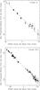 |
Fig. A.1 Sky-projected maser radii, derived from the ratio of the maser l.o.s. velocity with the angular velocity (see Sect. A), versus position projected along the major axis of the spatial distribution for the maser cluster “A” (upper panel) and the combined clusters “B” + “C” (lower panel). Dot size is proportional to the logarithm of the maser intensity and vertical errorbars give the estimated errors of the maser radii. The black dashed line denotes the “Y = X” axis. |
Acknowledgments
We are grateful to Dr. Q. Zhang for fuitful discussion on the kinematics traced by thermal molecular lines in the hot-core. We are also grateful to Dr. G. Surcis for useful discussion on the magnetic field traced by 6.7 GHz methanol masers in the region.
References
- Akabane, K., & Kuno, N. 2005, A&A, 431, 183 [NASA ADS] [CrossRef] [EDP Sciences] [Google Scholar]
- Banerjee, R., & Pudritz, R. E. 2007, ApJ, 660, 479 [NASA ADS] [CrossRef] [Google Scholar]
- Beltrán, M. T., Cesaroni, R., Neri, R., & Codella, C. 2011, A&A, 525, A151 [NASA ADS] [CrossRef] [EDP Sciences] [Google Scholar]
- Beuther, H., & Walsh, A. J. 2008, ApJ, 673, L55 [NASA ADS] [CrossRef] [Google Scholar]
- Beuther, H., Linz, H., & Henning, T. 2013, A&A, 558, A81 [NASA ADS] [CrossRef] [EDP Sciences] [Google Scholar]
- Bonnell, I. A., Bate, M. R., & Zinnecker, H. 1998, MNRAS, 298, 93 [NASA ADS] [CrossRef] [Google Scholar]
- Campbell, B. 1984, ApJ, 282, L27 [NASA ADS] [CrossRef] [Google Scholar]
- Cesaroni, R., Felli, M., Jenness, T., et al. 1999, A&A, 345, 949 [NASA ADS] [Google Scholar]
- Cesaroni, R., Galli, D., Lodato, G., Walmsley, M., & Zhang, Q. 2006, Nature, 444, 703 [NASA ADS] [CrossRef] [PubMed] [Google Scholar]
- Cotera, A. S., Whitney, B. A., Young, E., et al. 2001, ApJ, 556, 958 [NASA ADS] [CrossRef] [Google Scholar]
- Cragg, D. M., Sobolev, A. M., & Godfrey, P. D. 2005, MNRAS, 360, 533 [NASA ADS] [CrossRef] [Google Scholar]
- Davies, B., Hoare, M. G., Lumsden, S. L., et al. 2011, MNRAS, 416, 972 [NASA ADS] [CrossRef] [Google Scholar]
- De Buizer, J. M. 2003, MNRAS, 341, 277 [NASA ADS] [CrossRef] [Google Scholar]
- De Buizer, J. M., & Minier, V. 2005, ApJ, 628, L151 [NASA ADS] [CrossRef] [Google Scholar]
- De Buizer, J. M., Redman, R. O., Longmore, S. N., Caswell, J., & Feldman, P. A. 2009, A&A, 493, 127 [NASA ADS] [CrossRef] [EDP Sciences] [Google Scholar]
- Gaume, R. A., Goss, W. M., Dickel, H. R., Wilson, T. L., & Johnston, K. J. 1995, ApJ, 438, 776 [NASA ADS] [CrossRef] [Google Scholar]
- Goddi, C., & Moscadelli, L. 2006, A&A, 447, 577 [NASA ADS] [CrossRef] [EDP Sciences] [Google Scholar]
- Goddi, C., Moscadelli, L., Alef, W., et al. 2005, A&A, 432, 161 [NASA ADS] [CrossRef] [EDP Sciences] [Google Scholar]
- Goddi, C., Moscadelli, L., Torrelles, J. M., Uscanga, L., & Cesaroni, R. 2006, A&A, 447, L9 [NASA ADS] [CrossRef] [EDP Sciences] [Google Scholar]
- Goddi, C., Moscadelli, L., & Sanna, A. 2011, A&A, 535, L8 [NASA ADS] [CrossRef] [EDP Sciences] [Google Scholar]
- Keto, E., Zhang, Q., & Kurtz, S. 2008, ApJ, 672, 423 [NASA ADS] [CrossRef] [Google Scholar]
- Klaassen, P. D., Wilson, C. D., Keto, E. R., & Zhang, Q. 2009, ApJ, 703, 1308 [NASA ADS] [CrossRef] [Google Scholar]
- Koerner, D. W., & Sargent, A. I. 1995, AJ, 109, 2138 [NASA ADS] [CrossRef] [Google Scholar]
- Kraus, S., Balega, Y., Elitzur, M., et al. 2006, A&A, 455, 521 [NASA ADS] [CrossRef] [EDP Sciences] [Google Scholar]
- Kuiper, R., Klahr, H., Beuther, H., & Henning, T. 2010, ApJ, 722, 1556 [CrossRef] [Google Scholar]
- Kuiper, R., Klahr, H., Beuther, H., & Henning, T. 2011, ApJ, 732, 20 [NASA ADS] [CrossRef] [Google Scholar]
- Matthews, L. D., Greenhill, L. J., Goddi, C., et al. 2010, ApJ, 708, 80 [NASA ADS] [CrossRef] [Google Scholar]
- Minier, V., Booth, R. S., & Conway, J. E. 1998, A&A, 336, L5 [NASA ADS] [Google Scholar]
- Minier, V., Booth, R. S., & Conway, J. E. 2000, A&A, 362, 1093 [NASA ADS] [Google Scholar]
- Moscadelli, L., Goddi, C., Cesaroni, R., Beltrán, M. T., & Furuya, R. S. 2007, A&A, 472, 867 [NASA ADS] [CrossRef] [EDP Sciences] [Google Scholar]
- Moscadelli, L., Reid, M. J., Menten, K. M., et al. 2009, ApJ, 693, 406 [NASA ADS] [CrossRef] [Google Scholar]
- Moscadelli, L., Cesaroni, R., Rioja, M. J., Dodson, R., & Reid, M. J. 2011, A&A, 526, A66 [NASA ADS] [CrossRef] [EDP Sciences] [Google Scholar]
- Moscadelli, L., Li, J. J., Cesaroni, R., et al. 2013, A&A, 549, A122 [NASA ADS] [CrossRef] [EDP Sciences] [Google Scholar]
- Palla, F., & Stahler, S. W. 1993, ApJ, 418, 414 [NASA ADS] [CrossRef] [Google Scholar]
- Pestalozzi, M. R., Elitzur, M., Conway, J. E., & Booth, R. S. 2004, ApJ, 603, L113 [NASA ADS] [CrossRef] [Google Scholar]
- Pestalozzi, M., Jerkstrand, A., & Conway, J. 2012, in IAU Symp. 287, eds. R. S. Booth, W. H. T. Vlemmings, & E. M. L. Humphreys, 186 [Google Scholar]
- Qiu, K., Zhang, Q., & Menten, K. M. 2011, ApJ, 728, 6 [NASA ADS] [CrossRef] [Google Scholar]
- Sandell, G., Wright, M., & Forster, J. R. 2003, ApJ, 590, L45 [NASA ADS] [CrossRef] [Google Scholar]
- Sandell, G., Goss, W. M., Wright, M., & Corder, S. 2009, ApJ, 699, L31 [NASA ADS] [CrossRef] [Google Scholar]
- Sanna, A., Moscadelli, L., Cesaroni, R., et al. 2010a, A&A, 517, A71 [NASA ADS] [CrossRef] [EDP Sciences] [Google Scholar]
- Sanna, A., Moscadelli, L., Cesaroni, R., et al. 2010b, A&A, 517, A78 [NASA ADS] [CrossRef] [EDP Sciences] [Google Scholar]
- Seifried, D., Banerjee, R., Klessen, R. S., Duffin, D., & Pudritz, R. E. 2011, MNRAS, 417, 1054 [NASA ADS] [CrossRef] [Google Scholar]
- Sollins, P. K., & Ho, P. T. P. 2005, ApJ, 630, 987 [NASA ADS] [CrossRef] [Google Scholar]
- Surcis, G., Vlemmings, W. H. T., Torres, R. M., van Langevelde, H. J., & Hutawarakorn, K. B. 2011, A&A, 533, A47 [NASA ADS] [CrossRef] [EDP Sciences] [Google Scholar]
- Surcis, G., Vlemmings, W. H. T., van Langevelde, H. J., Hutawarakorn Kramer, B., & Quiroga-Nuñez, L. H. 2013, A&A, 556, A73 [NASA ADS] [CrossRef] [EDP Sciences] [Google Scholar]
- Torrelles, J. M., Patel, N. A., Anglada, G., et al. 2003, ApJ, 598, L115 [NASA ADS] [CrossRef] [Google Scholar]
- Torrelles, J. M., Patel, N. A., Curiel, S., et al. 2011, MNRAS, 410, 627 [NASA ADS] [CrossRef] [Google Scholar]
- Wynn-Williams, C. G., Becklin, E. E., & Neugebauer, G. 1974, ApJ, 187, 473 [NASA ADS] [CrossRef] [Google Scholar]
- Zhu, L., Zhao, J.-H., Wright, M., et al. 2013, ArXiv e-prints [Google Scholar]
- Zinnecker, H., & Yorke, H. W. 2007, ARA&A, 45, 481 [NASA ADS] [CrossRef] [Google Scholar]
All Tables
All Figures
|
Fig. 1 6.7 GHz CH3OH masers detected over three epochs with the EVN, overlaid on the 1.3 cm continuum imaged with the VLA A-Array. Colored dots show the absolute position of individual maser features, with color denoting the maser VLSR, according to the color-velocity conversion code reported on the right side of the panel4. Maser absolute positions are relative to the epoch 2005 September 9, which is the first of the five VLBA epochs used by Moscadelli et al. (2009) to measure absolute positions and proper motions of the 12 GHz CH3OH masers in NGC 7538 IRS1. Dot size is proportional to the logarithm of the maser intensity. Masers are grouped in different clusters, labeled using capital letters from “A” to “E”. The 1.3 cm map (dotted contours) was produced using archival data, originally reported by Gaume et al. (1995). Plotted contours are 7%, 10% to 90% (in steps of 10%), and 95% of the map peak, 0.022 Jy beam-1. Dotted arrows point to the main 1.3 cm continuum peaks, which are named following the notation by Gaume et al. (1995). The beam of the VLA-A 1.3 cm observations is reported in the insert in the bottom right of the panel. |
| In the text | |
|
Fig. 2 Proper motions of 6.7 GHz CH3OH masers detected over three epochs with the EVN. Symbols, colors and contours have the same meaning as in Fig. 1. The plotted field of view includes the maser clusters “A”, “B”, “C” and “D” (top panel), and cluster “E” (lower panel). Colored arrows show the measured maser proper motions, with dotted arrows denoting the most uncertain measurements. The scale for the proper motion amplitude is given by the black arrow in the lower left corner of each panel. |
| In the text | |
|
Fig. 3 Spectral profiles and time variation in peak velocities of selected maser features of cluster “A”. The plots in each column show a distinct maser feature in the cluster, labeled according to Table 2. (Top panels) Spectral profiles of maser features at different epochs, from Epoch 0 or Epoch 1 down to Epoch 3. The spectra (black dots) are produced by plotting the spot intensity vs. the spot channel velocity. For sufficiently well sampled maser spectra, the dotted curve shows the Gaussian profile fitted to the spectral emission. (Bottom panels) Plot of the maser peak velocity (with the associated errorbar) vs. the observing epoch (expressed in days elapsed from Epoch 0). The dotted line gives the least-square linear fit of velocities vs. time. |
| In the text | |
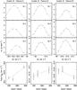 |
Fig. 4 Same as for Fig. 3 for cluster “B”. |
| In the text | |
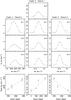 |
Fig. 5 Same as for Fig. 3 for cluster “C”. |
| In the text | |
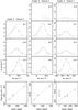 |
Fig. 6 Same as for Fig. 3 for cluster “D”. |
| In the text | |
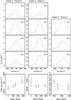 |
Fig. 7 Same as for Fig. 3 for cluster “E”. |
| In the text | |
|
Fig. 8 l.o.s. accelerations measured for individual 6.7 GHz maser features. Each panel shows a different cluster, from “A” to “E”. For each maser feature, the value of the l.o.s. acceleration is quoted in km s-1 yr-1. Symbols, colors and contours have the same meaning as in Fig. 1. In panels of the maser clusters “A”, “B” and “C”, the dashed line indicates the major axis of the maser feature’ spatial distribution, and the star marks the reference point to measure axis-projected offsets (see Sect. 4.1). |
| In the text | |
|
Fig. 9 Spectral profiles for NH3 inversion transitions (6,6), (7,7), (9,9), (10,10), and (13,13) observed toward NGC 7538 IRS1 with the JVLA B-Array. The upper panel is showing the spectra integrated over the core component of the 1.3 cm continuum emission (see Fig. 1), and the lower panel the spectra integrated towards the southern spherical component. An offset in flux density was applied to better evidence their spectral profiles. The velocity resolution is 0.4 km s-1 and the l.o.s. velocities are with respect to the local standard of rest (LSR). The dashed green (at −59.4 km s-1) and red (at −58.2 km s-1) lines indicate the central velocity of the least, (6,6), and most, (13,13), excited transitions, respectively, determined by fitting a single Gaussian to the transition spectral profile. In the southern component only the (6,6), (7,7), and (9,9) lines are clearly detected. The upper state energy levels of transitions shown here are ≈408–1693 K. |
| In the text | |
|
Fig. 10 Velocity fields of four inversion transitions of NH3, (6,6), (9,9), (10,10), and (13,13), as measured towards NGC 7538 IRS1 with the JVLA B-Array. In each panel, the positions of the 6.7 GHz CH3OH masers (black-circled, colored dots) are overlaid on the NH3 image. The conversion code between colors and VLSR is indicated in the wedge to the right side of the upper right panel. Dot size is proportional to the logarithm of the maser intensity. Dotted contours have the same meaning as in Fig. 1. In the bottom right panel, the labels of the maser clusters and the names of the main 1.3 cm continuum peaks are given. |
| In the text | |
|
Fig. 11 Linear fits to the spatial distributions of maser features in cluster “A”, and in the combined clusters “B” + “C” (dashed lines). Symbols, colors and contours have the same meaning as in Fig. 1. To fit the maser spatial distribution in these clusters, we have selected a subset of features closely aligned along the cluster major axis, excluding the subgroup of weak features scattered to the SE of cluster “A”, the subgroup of features of cluster “B” lying further south, and the subgroup in cluster “C” more detached to NW. The stars labeled IRS1a and IRS1b mark the YSO positions, as discussed in Sect. 6. |
| In the text | |
|
Fig. 12 Maser VLSR versus position projected along the major axis of the spatial distribution for the maser cluster(s) “A” (left panel) and “B” + “C” (right panel). The positional offsets are measured with respect to the YSO positions shown in Fig. 11. Maser (relative) positions and VLSR are known with an accuracy better than 1 mas (see Table 2) and 0.1 km s-1 (see Table 1), respectively. These plots are produced considering only the features closely aligned along the cluster major axis. Dot size is proportional to the logarithm of the maser intensity. The linear and quadratic fit to the plotted distribution is indicated with a black dashed and red dot-dashed line, respectively. |
| In the text | |
|
Fig. 13 Colored curves show strips of the first-moment map of different NH3 transitions, taken along the major axis of the maser clusters “A” (upper panel) and “B” + “C” (lower panel) . Colored bars along the “Y” axis mark the mean VLSR of the NH3 lines. The association color–NH3 transition is indicated in the upper left corner of the panel. Black dots report the 6.7 GHz masers of the clusters, selecting only the features closely aligned along the cluster major axis. Dot size is proportional to the logarithm of the maser intensity. The linear and quadratic fits to the maser distribution are indicated with a black dashed and black dot-dashed line, respectively. Colored dotted lines show the linear fits to the first-moment strips of the NH3 transitions. |
| In the text | |
|
Fig. 14 Emission centroids of NH3 fitted as a function of velocity (open squares) and CH3OH masers (filled circles) overlaid on the 1.3 cm continuum map (black image and white contours). Color denotes VLSR (color scale on the right-hand side). The sizes of squares and circles scale linearly and logarithmically with the flux density of NH3 and CH3OH maser emission, respectively. The relative alignment between NH3 and CH3OH is accurate to ~30 mas. Note that NH3 emission distributes between IRS1a and IRS1b, shows a velocity gradients roughly N–S, and is strongest towards IRS1a. |
| In the text | |
|
Fig. 15 The colored curves are the loci of the 6.7 GHz features, as derived from the edge-on disk model described in Sect. 5.2. We assume that the masers emerge from the near-side of the disk. Maser positions are described by the Eq. (14) (see Sect. 5), using the coefficients α = 7.1 10-5 km s-1 mas-2 and β = 0.020 km s-1 mas-1, derived in Sect. 4.1 fitting the change in maser VLSR with position in the clusters “B” + “C”. The colors black, red and blue identify the maser patterns corresponding to the values of the exponent q equal to 0, 1, and 2, respectively. Light squares, heavy solid line and light triangles are used to plot the curves corresponding to the values of the maser radius at the star position, R0 = 250, 500 and 750 AU, respectively. The star marks the location of the star at the disk centre. The magenta solid line indicates the linear change of the maser angular velocity Ω with the position projected along the cluster major axis. The two green bars mark the range of major-axis projected offset over which the 6.7 GHz masers of the clusters “B” + “C” distribute. Dashed arcs indicate circular orbits at steps of 200 AU in radial distance. |
| In the text | |
|
Fig. 16 Result of the model-fit for the cluster “A” (upper panel) and clusters “B” + “C” (lower panel). The colored map shows the distribution of χ2 (calculated using Eq. (20)) around the best-fit position, plotting values from the minimum of χ2 up to 50% above the minimum. The color-value conversion code is shown by the wedge on the right of the panel. The white cross shows the position of the minimum of χ2. The full white contours show levels of 10%, 20%, 30% and 40% above the minimum value of χ2. |
| In the text | |
|
Fig. 17 Comparison of the measurements and best-fit values for the cluster “A” (left panels) and clusters “B” + “C” (right panels). Upper and lower panels refer to the velocities (projected along the cluster major-axis) and the l.o.s. accelerations, respectively. Red crosses and errorbars give the measurements and corresponding errors, plotted vs. the maser position. The black dashed line shows the change of the model-predicted quantities along the maser pattern, with black crosses denoting the values in correspondence of the maser positions. |
| In the text | |
|
Fig. 18 Locations of maser features as derived from the edge-on disk model described in Sect. 5.2, assuming that the masers emerge from the near-side of the disk. Colored dots give the position for features of cluster(s) “A” (left panel) and “B” + “C” (right panel). For each cluster, only the maser features closely aligned along the cluster major axis are considered. Symbols and colors have the same meaning as in Fig. 1. The labeled star marks the YSO position at the disk centre. Dashed arcs indicate circular orbits at steps in radial distance of 500 and 200 AU, for the plot of cluster(s) “A” and ”B” + “C”, respectively. |
| In the text | |
|
Fig. A.1 Sky-projected maser radii, derived from the ratio of the maser l.o.s. velocity with the angular velocity (see Sect. A), versus position projected along the major axis of the spatial distribution for the maser cluster “A” (upper panel) and the combined clusters “B” + “C” (lower panel). Dot size is proportional to the logarithm of the maser intensity and vertical errorbars give the estimated errors of the maser radii. The black dashed line denotes the “Y = X” axis. |
| In the text | |
Current usage metrics show cumulative count of Article Views (full-text article views including HTML views, PDF and ePub downloads, according to the available data) and Abstracts Views on Vision4Press platform.
Data correspond to usage on the plateform after 2015. The current usage metrics is available 48-96 hours after online publication and is updated daily on week days.
Initial download of the metrics may take a while.