| Issue |
A&A
Volume 694, February 2025
|
|
|---|---|---|
| Article Number | A165 | |
| Number of page(s) | 20 | |
| Section | Extragalactic astronomy | |
| DOI | https://doi.org/10.1051/0004-6361/202452179 | |
| Published online | 11 February 2025 | |
X-ray view of a massive node of the Cosmic Web at z ∼ 3
I. An exceptional overdensity of rapidly accreting supermassive black holes
1
Dipartimento di Fisica “G. Occhialini”, Università degli Studi di Milano-Bicocca, Piazza della Scienza 3, I-20126 Milano, Italy
2
INAF – Osservatorio Astrofisco di Arcetri, Largo E. Fermi 5, 50127 Firenze, Italy
3
INAF – Osservatorio di Astrofisica e Scienza dello Spazio di Bologna, Via Piero Gobetti, 93/3, 40129 Bologna, Italy
4
Kapteyn Astronomical Institute, University of Groningen, Landleven 12, 9747 AD Groningen, The Netherlands
5
Dipartimento di Fisica, Università degli Studi di Torino, via Pietro Giuria 1, I-10125 Torino, Italy
6
Istituto Nazionale di Fisica Nucleare, Sezione di Torino, I-10125 Torino, Italy
7
Harvard-Smithsonian Center for Astrophysics, 60 Garden St., Cambridge, MA 02138, USA
8
INAF – Osservatorio Astronomico di Trieste, Via G. B. Tiepolo 11, 34143 Trieste, Italy
⋆ Corresponding author; This email address is being protected from spambots. You need JavaScript enabled to view it.
Received:
9
September
2024
Accepted:
12
December
2024
Abstract
Context. Exploring supermassive black hole (SMBH) populations in protoclusters offers valuable insights into how environment affects SMBH growth. However, research on active galactic nuclei (AGN) within these areas is still limited by the small number of protoclusters known at high redshift and by the availability of associated deep X-ray observations.
Aims. In order to understand how different environments affect AGN triggering and growth at high redshift, we investigated the X-ray AGN population in the field of the MUSE Quasar Nebula 01 (MQN01) protocluster at z ≃ 3.25. This field is known for hosting one of the largest Ly α nebulae and overdensities of UV continuum selected and sub-millimetre galaxies found so far at this redshift.
Methods. We conducted an ultra-deep Chandra X-ray survey (634 ks) observation of the MQN01 field and produced a comparative analyses of the properties of the X-ray AGN detected in MQN01 against those observed in other selected protoclusters, such as Spiderweb and SSA22.
Results. By combining the X-ray observations with deep MUSE and ALMA data of the same field, we identified six X-ray AGN within a volume of 16 comoving Mpc2 and ±1000 km s−1, corresponding to an X-ray AGN overdensity of δ ≈ 1000. This overdensity increases at the bright end (log(L2#x2212;10 keV/erg s−1) ≳ 44.5), exceeding what was observed in the Spiderweb and SSA22 within similar volumes. The AGN fraction measured in MQN01 is significantly higher (> 20%) than in the field and increases with stellar masses, reaching a value of 100% for log(M*/M⊙) > 10.5. Lastly, we observe that the average specific accretion rate (λsBHAR) for SMBH populations in MQN01 is higher than in the field and other protoclusters, generally increasing as one moves toward the centre of the overdense structures.
Conclusions. Our results, especially the large fraction of highly accreting SMBHs in the inner regions of the MQN01 overdensity, suggest that protocluster environments offer ideal physical conditions for SMBH triggering and growth.
Key words: galaxies: clusters: general / galaxies: high-redshift / quasars: general / quasars: supermassive black holes / X-rays: galaxies
© The Authors 2025
 Open Access article, published by EDP Sciences, under the terms of the Creative Commons Attribution License (https://creativecommons.org/licenses/by/4.0), which permits unrestricted use, distribution, and reproduction in any medium, provided the original work is properly cited.
This article is published in open access under the Subscribe to Open model. This email address is being protected from spambots. You need JavaScript enabled to view it. to support open access publication.
1. Introduction
The active phases of galactic nuclei (AGN) represent relatively short periods (≲0.1 Myr; King & Nixon 2015; Schawinski et al. 2015) in the life of a galaxy, during which the central supermassive black hole (SMBH) accretes mass. These brief episodes involve the release of a significant amount of energy, which are expected to influence the evolution of galaxies (Binney & Tabor 1995; Magorrian et al. 1998; Harrison & Ramos Almeida 2024, and references therein) and the surrounding gas on scales extending up to scales of hundreds of kiloparsecs (kpc) (Tytler et al. 1995; Fabian et al. 2003; Cicone et al. 2015; Travascio et al. 2020). The study of the AGN duty cycle, influenced by feeding and feedback processes, is crucial for understanding the role of these phases in galaxy evolution. Recent research by various authors (Bongiorno et al. 2012, 2016; Aird et al. 2012, 2018; Carraro et al. 2020) has explored the connection between SMBH accretion and galactic properties, focusing on the effects of AGN feedback on galactic quenching (e.g. Sturm et al. 2011; Dubois et al. 2013; Bongiorno et al. 2016) and the history of SMBH–galaxy co-evolution (Kormendy & Ho 2013). This co-evolution is key to explaining the local relationships observed between the masses of galactic bulges and SMBHs (Häring & Rix 2004), as well as the similar cosmic evolution trends of SMBH accretion density and star formation rate density (Boyle et al. 1998; Aird et al. 2015). The role of the environment adds another layer of complexity to this scenario. The AGN phase appears to be particularly significant in high-redshift overdense regions, where abundant gas reservoirs and high merger rates can promote SMBH growth and accelerate galaxy evolution (Martini et al. 2013; Assef et al. 2015; Hennawi et al. 2015; Marchesi et al. 2023; Vito et al. 2023; Elford et al. 2024). Studying the AGN activity in these environments is crucial to explore the growth of SMBHs over cosmic time and to achieve a comprehensive understanding of galaxy and large-scale structure evolution, as well as their complex interactions.
Those high-redshift overdensities that are identified as the progenitors, not yet virialized, of the massive (≳ 1014 M⊙) galaxy clusters observed in the local Universe, are defined as protoclusters (see Overzier 2016, and references therein). Various tracers are employed for identifying protoclusters. High-redshift radio galaxies, exhibiting extensive radio jets, were initially regarded as indicators of potential protoclusters (Carilli et al. 1997; Pentericci et al. 2000; Miley & De Breuck 2008; Hatch et al. 2014). Other proxies of protoclusters are significant overdensities of various types of galaxies, for example, Lyman-α emitters (LAEs), Lyman break galaxies (LBGs), and sub-millimetre galaxies (SMGs). The presence of large reservoirs of gas is also a key identifier of these structures. The hot phase of diffuse gas can be detected through extended X-ray emission (Gobat et al. 2011; Stanford et al. 2012; Tozzi et al. 2015; Champagne et al. 2021; Lepore et al. 2024) and the Sunyaev-Zel’dovich effect in sub-millimetre data (Gobat et al. 2019; Andreon et al. 2023; Di Mascolo et al. 2023; van Marrewijk et al. 2024), and its presence may be associated with large-scale shocked gas, or to high-density gas in virialized sub-halos within the protocluster. The warm phase (T ∼ 104 − 105 K) is revealed by the presence of extended Ly α emitting structures, typically powered by the photoionization of nearby AGN (e.g. Cantalupo et al. 2014; Hennawi et al. 2015; Arrigoni Battaia et al. 2018). In recent decades, the number of detected protoclusters has been increasing, primarily due to the refinement of selection techniques and the proliferation of surveys dedicated to this purpose (Cucciati et al. 2014; Toshikawa et al. 2016; Higuchi et al. 2019; da Costa & Menéndez-Delmestre 2021; Uchiyama et al. 2022).
Some progress has been made in the search for the AGN population within protoclusters. X-ray observations are crucial for probing AGN in these environments, as X-ray photons can penetrate high column density gas. This gas causes intrinsic obscuration of softer X-ray photons from the nuclear region and complete obscuration when NH ⪆ 1024 cm−2. Such obscuration is a common characteristic of AGN in dense regions (Menci et al. 2003; Hopkins et al. 2006; Assef et al. 2015; Vito et al. 2020). The X-ray Chandra telescope has played a pivotal role in identifying X-ray AGN at high redshifts, thanks to its high spatial resolution and sensitivity. Several studies (Lehmer et al. 2009; Digby-North et al. 2010; Macuga et al. 2019; Tozzi et al. 2022; Vito et al. 2024) conducted with over 200 ks of Chandra observations have provided evidence of enhanced X-ray nuclear activity in protoclusters compared to the field (Georgakakis et al. 2015; Ranalli et al. 2016; Vito et al. 2018), as well as to lower-redshift galaxy clusters (Martini et al. 2013). However, a more in-depth investigation into the effects of these environments on the AGN phase and vice versa requires a greater number of studies based on homogeneous multi-wavelength observations. Such comprehensive data are essential to reach robust conclusions.
This paper is the first contribution in a series dedicated to analyzing Chandra X-ray data of the Multi Unit Spectroscopic Explorer (MUSE) Quasar Nebula 01 (hereafter MQN01) field. This field was originally observed with the MUSE instrument on the Very Large Telescope (VLT) telescope, pointing one of the brightest Quasi Stellar Objects (QSOs) in the Universe, CTS G18.01 (λL1700 = 6.5 × 1046 erg s−1). Around it, Borisova et al. (2016) found one of the two largest (> 100 kpc) Ly α nebulae observed in their sample, potentially correlated with the presence of a protocluster structure. The existence of a protocluster in this field is also supported by numerous multi-wavelength observations acquired over the past three years, all aimed at investigating the galaxy population around this huge Ly α nebula. MUSE follow-up observations consisting of a mosaic of four frames, ∼10 h each one, was obtained in a ∼4 arcmin2 area around the QSO CTS G18.01 (PI Cantalupo, 0104.A-0203(A)). These deep MUSE observations reveal a Ly α emitting structure (Cantalupo et al., in prep.) more extended than the nebula originally discovered by Borisova et al. (2016). Moreover, the analysis conducted in Galbiati et al. (2024) revealed 21 galaxies embedded in the protocluster within ±1000 km s−1 from the bright QSO CTS G18.01, which was assumed to be the centre of the overdensity. This detection indicates an overdensity of ≃53 ± 17 of galaxies with a magnitude MR < −19.25 mag. Finally, the detection of six CO(4-3) emitting galaxies in this field, as probed by the Atacama Large Millimeter/sub-millimeter Array (ALMA) in Pensabene et al. (2024), indicates an overdensity of ≃15 ± 12. These high overdensities of spectroscopically selected protocluster members further confirm the existence of a protocluster in the MQN01 field. Additional rest-frame optical and near-UV images obtained from the Focal Reducer and low-dispersion Spectrograph 2 (FORS2), High Acuity Wide-field K-band Imager (HAWK-I) instruments mounted on the Very Large Telescope (VLT), Hubble Space Telescope (HST) with the F625W and F814W filters, and the James Webb Telescope using the NIRCam instrument, will be utilized in forthcoming publications to explore several properties of the galaxy population in the MQN01 protocluster (Galbiati et al. 2024; Wang et al., in prep.).
In this paper, we present an analysis of deep X-ray Chandra data obtained for the MQN01 field. We aim to conduct a comprehensive census of X-ray AGN, examining their X-ray luminosities, spatial distribution, and overdensity within the MQN01 protocluster. Additionally, we investigate the collective properties of these AGN, including their fraction relative to galaxies selected based on a stellar mass threshold, and the SMBH accretion rates as a function of environmental characteristics. To ensure an accurate interpretation of the effect of the environment on the AGN activity, these findings are compared with those observed in the field and other protoclusters.
The paper is organized as follows. Section 2 provides an overview of the Chandra X-ray observations, including a description of the data reduction and the detection of X-ray sources in the entire Chandra field. In Sect. 3 we present the ancillary multi-wavelength data used to support our selection of the X-ray sources associated with protocluster members. Section 4 presents the results from the spectral analysis of the X-ray emission from these protocluster members. Section 5 focuses on the collective properties of the AGN population in MQN01, including aspects such as compactness, the profile of the hard X-ray Luminosity Function, and the overdensity, all in comparison to the field and the AGN populations in two other protoclusters at z > 2, namely SSA22 and Spiderweb, which are introduced in Sect. 5.1 and for which deep (> 200 ks) Chandra observations have been analyzed in previous work. In Sect. 6 we explore potential correlations between galactic and environmental properties and SMBH activity, specifically investigating the variation of the AGN fraction as a function of stellar mass cuts for member galaxies, and the distribution of SMBH accretion rates in MQN01 and the other two protoclusters. The summary and conclusions are detailed in Sect. 8.
Throughout the paper, we adopted a cosmological model with H0 = 67.4 km s−1 Mpc−1, ΩΛ = 0.714, and Ωm = 0.286, consistent with the Planck Collaboration VI (2018) results. Under this cosmology, 1 arcsecond at z = 3.25 corresponds to a physical scale of 7.663 kpc. The uncertainties presented in all the plots correspond to a 1σ confidence level, unless otherwise specified1.
2. Chandra data: Reduction and analysis
2.1. Chandra data
We analyzed observations taken with the X-ray Chandra Advanced CCD Imaging Spectrometer (ACIS-I), optimized for imaging wide fields, during Cycle 23 in 2022/2023, with a cumulative exposure time of 634 ks (PI: S. Cantalupo). These observations were conducted in the Very Faint (VFAINT) mode, which enables a better distinction between good and bad X-ray events by utilizing the 5 × 5 pixel event island. A list of the ObsIDs and their corresponding pre-data reduction exposure times is provided in Table 1. Figure 1 shows the combined 0.5–7.0 keV image from Chandra observations, smoothed with a ∼1.5 arcsec Gaussian filter, with each ObsID observation indicated by a yellow square. We overlay the fields of view of the ancillary data used in this paper to compile a comprehensive census of X-ray AGN associated with the protocluster members. Further details on these data are provided in Sect. 3.1.
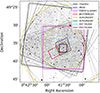 |
Fig. 1. Chandra X-ray image in the 0.5–7.0 keV energy band, smoothed with a ∼1.5 arcsec Gaussian filter. The black squares mark the individual ObsIDs of the Chandra observations detailed in Table 1. The dashed gold lines represent concentric circles centred on the aim point in the final merged image, with radii of 6 and 12 arcminutes. Additional contours delineate the areas of multi-wavelength observations, the details of which are outlined in Sect. 3.1. |
Chandra observation log.
2.2. Data reduction, alignment, and merging of the observations
Data reduction was carried out for each individual Chandra ObsID using CIAO 4.15 and the Chandra Calibration Database (CALDB-4.10.2) installed on Python 3.10. For the level 1 event files, we applied the destreak procedure to eliminate streak events along the pixel rows. Subsequently, we employed acis_build_badpix and acis_find_afterglow to generate a bad pixel file and identify events potentially associated with residuals from cosmic rays. Given that the observations were conducted in VFAINT mode, we set the parameter check_vf_pha = yes for a more accurate background cleaning. The event files were then filtered for standard event grades of 0, 2, 3, 4, and 6. A visual inspection was conducted on these event files to identify hot pixels and assess pile-up effects. Then the acis_process_events tool was used to update the data and correct for the effects of temperature-dependent charge-transfer inefficiency (CTI). We run wavdetect on each chip in the individual ObsID, setting the scale parameter to 2, 4, and 8, and the detection threshold to 1e-07. We used wavdetect output to identify the positions of X-ray detections, which were subsequently removed from the event files to generate new event files containing only background emission. From these files, we extracted light curves with a time binning of 100 s. Hence, we utilized deflare to filter the original event files for time intervals in which the background exceeds the average value by 3σ, after applying a clipping algorithm. Finally, all the chips were merged using the dmmerge tool. Following the filtering of dead-time due to flares identified in light curves we obtained a final dataset with exposure time of ∼634 ks. Finally, we created the aspect solution files for each CCD using asphist, and we utilized the mkinstmap and mkexpmap tools on individual chips and ObsID to generate monochromatic exposure maps at 1.5 and 4.5 keV.
To align the astrometry of each ObsID, we used flux_obs and mkpsfmap tools, to create the broad energy band (0.5–7.0 keV) images and the point spread function (PSF) maps at the energy 2.3 keV, respectively. The PSF map was weighted according to exposure times (i.e. psfmerge = “exptime”), with each pixel’s value representing the PSF radius containing an Encircled Counts Fraction (ECF) of 0.393 (i.e. psfecf = 0.393). These products were used to identify X-ray detections with wavdetect, setting the wavelet scale following the  -sigma series2 and specifying that we expect one false source rate per scale by setting falsesrc = 1. We used the positions of the sources in common between different observations, using as reference the deepest ObsID 25728, to reproject the event files, the monochromatic exposure maps weighted by time (unit = cm2), and the aspect solution files, using the wcs_match and wcs_update tools. This allowed us to align the different ObsID that will be merged. Subsequently, we used the GAIA catalog to correct the astrometry of the merged event file, initially showing a shift with respect to the GAIA sources of ≈0.55″.
After aligning the aspect files and performing the astrometric correction, we combined the monochromatic exposure maps using the corresponding exposure times as weights, and a merged event file from all the ObsIDs was then obtained by applying reproject_obs. Figure 1 displays the smoothed image with a 3-pixel kernel radius in the 0.5–7.0 keV energy band of the merged event file. The aim point of the merged event file was determined from the monochromatic exposure map at 1.5 keV as the position of the peak value (RAaim point = 10.3801543 deg, Decaim point = –49.6043256 deg). Figure 1 displays two circles centred at the aim point, with radii of 6 and 12 arcmin. A radius of 6 arcmin is equivalent to ≈2.8 pMpc (i.e. 11.9 cMpc at z = 3.25).
2.3. X-ray sources detection
Our main objective is to obtain a catalog of X-ray sources in the 4 arcmin2 region covered by the MUSE FoV, centred on the aim point of the Chandra observations because only in that region we have spectroscopically confirmed protocluster members. We used wavdetect to produce a complete catalog of Chandra X-ray sources in this region, minimizing false and missed detections. The wavdetect tool was run by setting the false-positive probability threshold to 10−5 (i.e. falsesrc = –1 and sigthresh = 1e-5), and the scale parameter to scales = “1 1.41 2 2.83 4 5.66 8 11.31 16”. Using this value for the threshold sigthresh, we expected ≈17 detections of background fluctuations within a 6 arcmin radius from the aim point. This process results in X-ray point-source catalogs, with 210 X-ray sources in the soft energy band, 313 in the broadband, and 275 in the hard band. We combined these three catalogs to generate a master catalog comprising 360 X-ray point sources detected in at least one energy band. A more detailed selection using a signal-to-noise (S/N) threshold identified 311 sources with S/N > 2 and 213 with S/N > 3. However, this selection does not affect our results, which focus on the MUSE mosaic FoV near the aim point. This more detailed analysis will be presented in future studies, aiming to investigate the X-ray counterparts of galaxies in a wider area than that of the MUSE mosaic FoV.
2.4. Sky coverage and number of counts
Given that one of the objectives of this paper is to explore the density of any X-ray AGN population in the protocluster MQN01, it is necessary to determine the sky coverage (Ω) of these Chandra observations (i.e. the area covered at a given sensitivity). The first step to obtain the sky coverage curve consists of estimating the conversion factors from count rate to fluxes, in different energy bands. The conversion factors were computed by generating ancillary response files (ARFs) and redistribution matrix files (RMFs) at the aim point using the mkwarf and mkrmf tools, respectively, for individual ObsID event files. ARFs and RMFs data were used to simulate one hundred high-S/N spectra of an X-ray source positioned at the aim point using the fake_pha tool in Sherpa (Freeman et al. 2001), a software package integrated within CIAO and operated via Python. The spectral emission is assumed to follow a power-law distribution with a photon index (Γ) ranging between 1.2 and 1.9, encompassing both absorbed (Γ < 1.7) and unabsorbed (Γ > 1.7) AGN (Lanzuisi et al. 2013; Liu et al. 2017). Therefore, for each ObsID, the conversion factor at the aim point within a specific energy band was determined as the ratio between the integrated flux (in erg cm−2 s−1) and the net count rate (in counts s−1). These values were obtained from the spectrum utilizing the tools calc_energy_flux and calc_model_sum. The final conversion factors and their associated errors, which are reported in Table 2, were computed as the average and standard deviation, respectively, across the conversion factors obtained for different Γ, ObsIDs, and energy ranges.
Conversion factors were calculated at the aimpoint and were used to convert any count rate in the energy band listed in Col. 1 to a photometric flux in the energy band listed in Col. 2.
To generate the curves of sky coverage (black lines in Fig. 2), we adopted a completeness criterion of S/N > 2, ensuring high significance detection (see Giacconi et al. 2001; Tozzi et al. 2001), and considering the observational solid angle within which ideal X-ray sources are detected above a specific flux. The S/N was calculated based on the net counts estimated in each region of the Chandra observation assuming a specific flux. We multiplied the flux of each X-ray source by the exposure time and the effective area value, observed in the 1.5 and 4.5 keV monochromatic exposure maps, at that position. The effective area was normalized to the value observed at the aim point. This product was then divided by the conversion factor, yielding the expected net counts associated with an ideal X-ray source with a specific flux. Hence, we quantified the associated solid angle, for each specific flux, according to the number of X-ray sources candidates observed with S/N > 2, based on the local background. In Fig. 2 we report the sky coverage curves for the Chandra Deep Field-South (CDFS; dashed lines, Rosati et al. 2002; Luo et al. 2017, 7 Ms), which is the field with the deepest X-ray data collected to date, and for other deep (texp > 400 ks) Chandra observations obtained for two other protoclusters: SSA22 (dotted lines; Lehmer et al. 2009, 400 ks) and Spiderweb (solid lines; Tozzi et al. 2022, 700 ks). These estimates encompass areas with varying solid angles and exposure times. The black and red curves represent the sky coverage for soft (0.5–2.0 keV) and hard (2.0–7.0 keV) fluxes, respectively. The soft and hard flux limits of our observations, defined as those observed within a minimum solid angle Ωmin = 2 × 10⁻³ deg2 equivalent to one-tenth of the full FoV, are 1.7 and 2.9 × 10⁻¹⁶ erg s−1 cm−2, respectively. The hard energy flux limits of the observations in all the protoclusters are very similar to each other, about one order of magnitude higher than those in the CDFS observations. In the soft band, the flux limit of our observations is about 3 and 1.5 times higher than those in Spiderweb and SSA22 observations, respectively, and ∼20 times larger than those in the 7 Ms CDFS observations. These differences are due to the combination of the different exposure times of the observations in the various fields, and the decreasing Chandra’s effective area in the soft band with time.
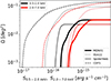 |
Fig. 2. Point source sky coverage for different Chandra observations in the soft (0.5–2.0 keV; black) and hard (2.0–7.0 keV; red) energy band. The thick solid lines mark the sky coverage of this study, while the thin solid, dotted, and dashed lines depict the sky coverage in the Chandra observations respectivley of Spiderweb (Tozzi et al. 2022), SSA22 (Lehmer et al. 2009), and Deep Field South (Rosati et al. 2002; Luo et al. 2017). |
Figure 3 displays the cumulative number counts N(> S) in the 0.5–2.0 (left) and 2.0–10.0 keV (right) energy bands, of detected X-ray sources in our Chandra observations within 6 arcminutes from the aim point, derived as in Rosati et al. (2002) (see also Luo et al. 2017; Tozzi et al. 2022). The shaded areas show the 2σ uncertainties derived by propagating the photometric flux errors of the sources. The black lines are the prediction from the AGN+Galaxy model developed in Gilli et al. (2007) using the “X-ray AGN number counts calculator” in the CXB tool3 by taking into account the decline of the AGN number density as a function of redshift. We noticed that the presence of a protocluster does not impact the number counts. Hence, the AGN enhancement that we identified, as will be shown in the following sections, lacks significance in amplitude to identify the protocluster as an excess in X-ray counts onto the X-ray sky due to the low statistics. This finding aligns with the results of previous studies analyzing Chandra data in SSA22 and Spiderweb protoclusters (Lehmer et al. 2009; Tozzi et al. 2022).
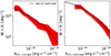 |
Fig. 3. Cumulative number of counts in the soft (left) and hard (2–10 keV; right) energy band, derived within a distance of 6 arcmin from the aim point in the Chandra data of MQN01. The red shaded area shows the uncertainties within 1σ due to photometric errors. The black line shows the number of counts predicted for the field from the AGN+Galaxy models developed in Gilli et al. (2007). |
3. Probing X-ray emission in the MQN01 protocluster: A comprehensive data overview and cross-matching strategy
We present an analysis aimed at associating Chandra X-ray sources with spectroscopically selected protocluster members, as identified in previous (Pensabene et al. 2024) and ongoing studies (Galbiati et al. 2024).
3.1. Ancillary data
In recent years, the MQN01 field has been observed using various telescopes and instruments across a wide range of wavelengths. Our analysis of X-ray Chandra data will leverage on the catalog of protocluster members spectroscopically selected through ALMA and MUSE observations. Additionally, we consider galactic properties, such as stellar mass (M*) and star formation rate (SFR), derived through spectral energy distribution (SED) fitting analysis using all available photometric flux measurements. Detailed descriptions of these observations and the respective analyses are provided below.
3.1.1. Spectroscopic data: VLT/MUSE and ALMA
VLT/MUSE-WFM Adaptive Optics (AO) observations are obtained from the Guaranteed Time Observation (GTO) program (PI S. Cantalupo), amounting to a cumulative observation time of 40 hours. These observations consist of a mosaic of four pointings, each with a duration of 10 hours, and covering a FoV of ∼2 × 2 arcmin2 shown with a blue contour in Fig. 1. Galbiati et al. (2024) identifies spectroscopically selected protocluster members in the MUSE FoV, based on the presence of multiple high-S/N emission and/or absorption lines. They found 21 galaxies within ±1000 km s−1 of the redshift of the QSO CTS G18.01, which was excluded from their analysis.
The contours in orange and green in Fig. 1 delineate the FoV of ALMA 12 m array data, which were obtained respectively in Band 3 (centred at 2.94 mm) and Band 6 (centred at 1.26 mm) during Cycle 8 (Program ID: 2021.1.00793.S, PI: S. Cantalupo). These data have been analyzed in Pensabene et al. (2024), revealing the presence of six CO(4-3) emitters within |δvQSO| < 1000 km s−1.
3.1.2. Photometric observations: VLT/FORS2, HST, JWST/NIRCam, and VLT/HAWK-I
The magenta square in Fig. 1 marks the FoV of images taken with the Focal Reducer and low-dispersion Spectrograph 2 mounted on the Very Large Telescope (VLT/FORS2), in U (λcen = 361 nm), B (λcen = 440 nm) and R (λcen = 655 nm) filters with on-source exposure times of ∼7 h, 5 h and 0.75 h, respectively. In the same area where FORS2 data were collected, HAWK-I images were obtained (programme ID 110.23ZX, PI S.Cantalupo) using CH4 (λeff = 1.575 μm), H (λeff = 1.620 μm), and Ks (λeff = 2.146 μm) filters, each with exposure times of 1 hour, 2 hours, and 2 hours on source, respectively. Furthermore, observations covering 2 × 5 arcmin2 (depicted by red squares in Fig. 1) were conducted with the James Webb Space Telescope (JWST) using the extra-wide filters F150W2 (0.6 − 2.3 μm; pixel scale of 0.031 arcsec/pixel) and F322W2 (2.4 − 5.0 μm; pixel scale of 0.063 arcsec/pixel). These observations were acquired under GO Cycle 1 program ID 1835 (PI S. Cantalupo), with a single pointing for each filter and an exposure time of 27 minutes. Additionally, HST/ACS observations (PI: S. Cantalupo, PID: 17065) were taken, during cycle 30, with the ACS F625W and F814W filters, depicted by cyan and purple squares in Fig. 1, respectively.
Galbiati et al. (2024) conducted a broad photometric selection of candidates at z = 3 − 3.5 using the FORS UBR-selection criterion based on BPASS models plus IGM transmission, as described in Steidel et al. (2018). This selection identified 30 potential protocluster candidates in the MUSE FoV, out of which 12 have confirmed spectroscopic redshifts obtained from VLT/MUSE observations. Galbiati et al. (2024) estimated the stellar mass (M*) and star formation rate (SFR) values for all the spectroscopically selected galaxies, using all the available multi-wavelength data (i.e. MUSE, VLT/FORS2, VLT/HAWK-I, ALMA, and HST/ACS). Specifically, HAWK-I data are very important for constraining the stellar masses of the galaxies embedded in the protocluster and for selecting Balmer-Break galaxies. The SEDs were fitted using the Code Investigating GALaxy Emission (CIGALE) with Bruzual & Charlot (2003) stellar population models, a Chabrier (2003) Initial Mass Function (IMF), and the Calzetti et al. (2000) dust law, while separating AGN and host galaxy contributions. For sources detected in X-rays, Galbiati et al. (2024) show that AGN contribution to the rest-frame optical emission is negligible by analyzing their morphology in JWST/NIRCam data, where none showed compact central emission. Uncertainties were estimated based on photometric and model systematics. High-resolution HST (FWHM = 0.12″) and JWST (FWHM ∼ 0.045 − 0.1″) images will be crucial for exploring the morphology of galaxies and correlating them with the large-scale environment.
3.2. Cross-matching Chandra data with multi-wavelength datasets
The primary aim of this section is to compile a comprehensive census of X-ray sources associated with galaxies embedded into the MQN01 protocluster. The redshift of the protocluster is set to that of the QSO CTS G18.01, which is zMQN01 = 3.2502 as determined by the CO(4-3) line detected in ALMA data (Pensabene et al. 2024). To achieve this objective, we conducted a cross-match between the X-ray source catalog, detailed in Sect. 2.3, and the spectroscopically selected protocluster members detected with MUSE and ALMA in their FoV. The X-ray emission is associated with a specific galaxy if the centroid offset is less than 0.5 arcseconds. This threshold is similar to the Chandra PSF (FWHM ≈ 0.5 arcsec) and smaller than that of WFM-AO MUSE PSF (FWHM ≈ 0.8 arcsec). Using this approach we found six X-ray sources associated with galaxies embedded into the MQN01 protoclusters.
Figure 4 presents the 2-pixel Gaussian kernel-convolved Chandra X-ray image at 0.2–10 keV (left panel) and the MUSE white-light image (WLI) (right panel). The blue dashed contours in the left panel outline the FoV of the MUSE mosaic shown on the right. In both panels, spectroscopically selected protocluster members identified with MUSE and ALMA are marked with cyan and blue circles, while red squares indicate the six X-ray sources associated with protocluster members, each labelled with an ID number (ID1-6).
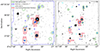 |
Fig. 4. Chandra X-ray and MUSE images of the MUSE field with symbols marking Chandra X-ray point sources and MQN01 protocluster membership candidates identified through spectroscopic and photometric methods. On the left, a 2 pixel Gaussian kernel-convolved image at the energy band of 0.5–10 keV, zoomed into the MUSE FoV (blue dashed square and blue square in Fig. 1). The red squares mark the X-ray point sources detected with S/N ≥ 3, each associated with an identity number. The blue and cyan circles show the spectroscopically confirmed MQN01 protocluster members within ±1500 km s−1 from the QSO CTS G18.01 (ID1) from MUSE (Galbiati et al. 2024) and within ±4000 km s−1 from ALMA (Pensabene et al. 2024), respectively. The green circles indicate the positions of FORS photometrically selected protocluster member candidates (Galbiati et al. 2024). The right panel shows the MUSE White Light Image of the same field with the same markers for multi-wavelength selections. |
ID1 corresponds to the bright QSO CTS G18.01. ID2 is the second brightest X-ray emission detected in this area. The remaining X-ray sources are numbered sequentially, with ID3 representing the northernmost source and ID6 representing the southernmost one. ID3 and ID4 are two closely positioned X-ray sources (∼2 arcsec) that can be easily de-blended, partly due to their different energy flux distributions. ID5 is associated with a compact galaxy. ID6 is associated with a very large disc galaxy observed with JWST/NIRCam data and confirmed as a protocluster member based on the spectroscopic redshift revealed by JWST/NIRSpec slit spectroscopic data and ALMA (Wang et al., in prep.). A zoom-in on these X-ray emissions at different energy bands, along with the circles marking the galaxies selected as protocluster members, is presented in Fig. A.1. All six X-ray detections are associated with galaxies that were spectroscopically selected with MUSE and ALMA, within a velocity range of ±1000 km s−1 of the redshift of the QSO CTS G18.01. Four of these X-ray sources are associated with CO(4-3) emitting-line galaxies (i.e. ID1, ID2, ID3, ID6), and ID3 is also associated with a CO(9-8) emission line (Pensabene et al. 2024).
Throughout this paper, we have focused exclusively on the sample of X-ray sources associated with spectroscopically selected galaxies. However, to gain a rough estimate of the potential number of X-ray sources among photometrically selected galaxies, we expanded our research on X-ray emission in protocluster members by including candidates selected with FORS as LBGs at 3 < z < 3.5 using the UBR-selection method (Galbiati et al. 2024). These sources are located within the FORS FoV shown as a magenta square in Fig. 1. We found that only one source out of 178, representing 0.6% of the sample, is associated with an X-ray detection with an offset of less than 0.5 arcseconds. This single case is located outside the MUSE FoV, positioned 3.6 arcmin away from CTS G18.01. The remarkably low percentage of X-ray counterparts associated with photometrically selected LBGs at z ≈ 3 − 3.5 is due to the ineffectiveness of the UBR-selection method to include LBGs that host an AGN (Galbiati et al. 2024). None of the spectroscopically selected galaxies associated with an X-ray emission is also selected as an LBG. Three X-ray sources are identified within the MUSE FOV and are not associated with any spectroscopically selected protocluster member (see the left panel in Fig. 4). One of these sources is linked to a galaxy with clear emission lines, constraining its redshift to z ≃ 3.8. The other sources are linked to galaxies that do not exhibit high-S/N emission lines.
In summary, our cross-matching analysis revealed X-ray emission in six spectroscopically selected protocluster members, inside the MUSE FoV region of 4 arcmin2 (equivalent to ∼4 cMpc × 4 cMpc at the redshift of the protocluster) and within ±1000 km s−1 from the central QSO, including X-ray emission of the QSO itself.
4. Spectroscopic analysis of X-ray sources in the MQN01 protocluster
We performed a spectral analysis of the X-ray sources associated with MQN01 protocluster members. At first, we extracted the spectra from circular regions with 2 times a radius defined as rext = (2.55 × 0.67791 − 0.0405083 θ + 0.0535066 θ2) arcsec in (which ensures that at least 95% of the expected source flux is included; Rosati et al. 2002, and references therein). There is an exception for the extraction of the spectrum of the blended sources ID3 and ID4, for which we used a radius 2rext/3, that is smaller than half the distance between the two X-ray sources, to avoid contamination between the two sources. The background regions, free of sources, were manually selected near each respective source in more extended circles whose radius ranges from 5 to 10 times the defined rext. Through the specextract tool, we obtained the ancillary response file (ARF) and the redistribution matrix file (RMF) at the source position, and the area- and exposure-weighted combination of source (.pi) and background (.bkg) spectra. For the spectral fitting analysis, we used XSPEC, by setting a C-statistic (Arnaud 1996). We adopted a simple model tbabs*(zphabs*pow) consisting of a power law convolved with a Galactic and intrinsic absorption. The Galactic absorption tbabs is set to NH, Gal = 1.18 × 1020 cm−2 according to the NASA HEASARC tool at the aim point coordinate within 0.1 deg. For the sources with net counts exceeding 100 (i.e. ID1 and ID2) we initially included an iron K-α line at the rest frame energy of 6.4 keV, left free to vary within the redshift uncertainties, and we left the slope Γ of the intrinsic power law free. In all cases, we observed that the iron K-α line is poorly constrained and, therefore, it was removed from the spectral model. For the rest of the sources, we assumed an intrinsic power-law slope Γ = 1.8, and only the power-law normalization and hydrogen column densities (NH) are free parameters.
Figure A.2 illustrates the spectra and best-fit models of these six X-ray sources. Table 3 shows the coordinates and redshifts of the X-ray protocluster members estimated from MUSE and/or ALMA data, along with the best-fit properties derived from the spectral analysis. These properties include the intrinsic NH, Γ, and the unabsorbed luminosities at the rest frame energy of2–10 keV (L2 − 10 keV), along with their respective 90% confidence levels. The luminosities were derived by applying a convolution model to the intrinsic power law by using the clumin tool in XSPEC. We observe that all X-ray protocluster members exhibit log(L2#x2212;10 keV/erg s−1) > 43.5 which indicates their classification as AGN (see Ueda et al. 2014).
Properties of the X-ray source candidates and the results from the best spectral-fit models.
In summary, we found that all detected X-ray sources within the MQN01 protocluster are associated with AGN activity. Two of these sources exhibit an obscuration level surpassing NH > 1023 cm−2, while for the remainder the obscuration is presumably lower, as indicated by unconstrained upper limit values of NH. A more detailed X-ray spectral analysis of the central QSO, also including a thermal component, will be presented in the next paper. In this work, our spectral analysis is only finalized in obtaining unabsorbed luminosities for all the X-ray AGN.
5. Spatial distribution, luminosity function, and overdensity of X-ray AGN in MQN01 and other protoclusters
5.1. Comparative analyses: AGN population in MQN01, SSA22, and Spiderweb protoclusters
Protoclusters have been identified across epochs spanning from z ∼ 1.6 to z = 8 (see Overzier 2016, for a review). Studying their AGN population, including characterizing their distribution, spatial density, and individual properties, offers insight into the evolution of SMBH growth about the development of these large-scale overdense structures. It also is crucial to reveal the role played by potentially enhanced feeding processes in these regions in promoting SMBH accretion. These compelling questions motivated our exploration, in this first paper, of the collective properties of the X-ray AGN population in the z ∼ 3.247 protocluster MQN01, including its spatial and velocity distribution, overdensity, AGN fraction, and SMBH accretion rates. To investigate any connection between the environment and the AGN population, these characteristics need to be compared to those in the field and other protoclusters. This comparison is challenging due to the limited number of homogeneous and robust studies of AGN populations in protoclusters. For this purpose, we considered two well-studied protoclusters: SSA22 and Spiderweb.
The SSA22 protocluster (Cowie et al. 1994; Steidel et al. 1998) provides an excellent comparative case for MQN01, because of a similar redshift (z ∼ 3.09). Furthermore, a 6 arcmin2 area is covered with the VLT/MUSE instrument, and, similar to MQN01, these observations have revealed the presence of extended Ly α filamentary structures (Umehata et al. 2019). A significant difference is the absence of a brightest QSO in SSA22, which could serve as a proxy for the minimum potential well position of the overdensity. The other protocluster that we included in this comparative analysis is Spiderweb. This is a structure centred on the bright high-redshift radio galaxy PKS 1138 at z ≃ 2.156 and represents a prototypical protocluster. Similar to the MQN01 and SSA22 fields, the Spiderweb protocluster also hosts an extended (≳200 kpc) Ly α nebula (Pentericci et al. 1997). Both the SSA22 and Spiderweb fields have been extensively studied with multi-wavelength observations, revealing several members down to Mpc scales. For instance, Steidel et al. (1998) discovered a highly significant concentration of 15 LBGs in the SSA22 protocluster. An LAEs overdensity of about six was identified within an area of ≃8.8 × 8.9 arcmin2, or ≃284 cMpc2 (Steidel et al. 2000; Yamada et al. 2012). In the Spiderweb protocluster, an overdensity of spectroscopically confirmed LAEs (Kurk et al. 2000; Pentericci et al. 2000) and Hα emitters (HAEs; Hatch et al. 2011; Kuiper et al. 2011; Shimakawa et al. 2015; Pérez-Martínez et al. 2023) has been found, covering areas of ∼111 cMpc2. Conversely, in the MQN01 field, an overdensity of spectroscopically confirmed protocluster members has been identified within the MUSE-mosaic FOV, covering approximately 4 × 4 cMpc2 (equivalent to ∼2 × 2 arcmin2), indicated by multiple high-S/N absorption and emission features (Galbiati et al. 2024, see our Sect. 3.1 for details). Therefore, the differences in the selection methods for identifying members and the different spectroscopic data coverages in these three protoclusters prevent the possibility of using consistent physical methods to derive comparable volumes and imply that the comparison should be taken with some caution.
On the other hand, deep Chandra observations available for these protoclusters, specifically with a total exposure time of approximately ∼400 ks for SSA22 (Lehmer et al. 2009) and ∼700 ks for Spiderweb (Tozzi et al. 2022), provide similar hard flux sensitivity to those in this paper, as shown in Fig. 2. Lehmer et al. (2009) identified ten AGN in SSA22 associated with LAEs and LBGs. Six of these AGN are associated with spectroscopically selected protocluster members at z ∼ 3.1, while two are located well beyond ±15 000 km s−1 from the protocluster redshift, and the remaining two are associated with only photometrically selected LBGs. Tozzi et al. (2022) identified 14 X-ray AGN in Spiderweb, including the central radio-jet galaxy PKS 1138 (Roettgering et al. 1994). One of these AGN is a candidate member based on X-ray data without spectroscopic confirmation, and two are Compton-Thick candidates, for which only the absorbed luminosity can be provided. Table 4 reports various properties of these protoclusters, their AGN populations, and the exposure times of the respective Chandra observations. In Col. 4 we report the number of X-ray AGN, associated with a spectroscopically selected galaxy within ±4000 km s−1 from the protocluster redshift (Col. 3), and in the brackets, we report those associated with photometrically selected protocluster member candidates.
Physical properties of the MQN01, SSA22, and Spiderweb protoclusters and their AGN populations.
5.2. AGN spatial distribution within protoclusters
The compactness of the AGN population in different environments provides insight into SMBH feeding processes and the potential extent of their feedback effects. We wondered whether the same compactness of AGN found in MQN01 was also present in the other two protoclusters. To address this question, we assumed that the centre of these protoclusters coincides with the region of the highest galaxy overdensity.
The histograms in Fig. 5 illustrate the velocity distribution of spectroscopically selected galaxies (white) and those hosting AGN (red) within ±4000 km s−1 of the redshift of each protocluster. These distributions are shown for galaxies within the specified areas indicated at the top left of each panel for each protocluster. Naturally, a larger survey area from which protocluster member galaxies are selected leads to a greater number of galaxies and a broader velocity distribution. The top panel shows the case for MQN01, the middle panel displays data for the Spiderweb protocluster, with galaxies detected in several studies (Pentericci et al. 2000; Kurk et al. 2004a; Croft et al. 2005; Kuiper et al. 2011; Tanaka et al. 2013; Dannerbauer et al. 2014; Shimakawa et al. 2018; Jin et al. 2021), and the bottom panel shows the distribution of galaxies associated with the SSA22 protocluster as collected by Mawatari et al. (2023). The redshifts of the protoclusters were obtained as the mean redshift of all galaxies within a ±1000 km s−1 range from an initial protocluster redshift (i.e. 3.25, 3.09, and 2.156 for MQN01, Spiderweb, and SSA22, respectively), according to the literature. These estimates allow an excellent centring on the peak of galaxies in velocity distribution and are listed in Col. 3 in Table 4. The AGN velocity distribution in MQN01 appears to be more compact compared to those in SSA22 and Spiderweb, with velocity ranges of 689 km s−1, 1610 km s−1, and 1830 km s−1, respectively (as reported in Col. 5 of Table 4). After that, we derived the spatial distribution of the AGN within ±4000 km s−1 from the protocluster redshift by measuring the area of circles with diameters equal to the maximum projected distance between X-ray AGN. We found areas of approximately 4.2, 463, and 77 cMpc2 for the MQN01, SSA22, and Spiderweb protoclusters, respectively (see Col. 6 of Table 4). These estimates of velocity and spatial distributions reflect the maximum extent of the AGN populations found in the three protoclusters, which is largely dependent on the available observations.
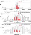 |
Fig. 5. Velocity distribution of the galaxies+AGN (white) and AGN (red) members of the MQN01 (top panel), Spiderweb (middle panel), and SSA22 (bottom panel) protoclusters, in a velocity range ±4000 km s−1 and within areas of approximately 16, 75, and 2400 cMpc2, respectively, as reported in the top left legend of each panel. |
To evaluate the compactness of active galaxy populations independently of the spectroscopic survey areas and the overall distribution of the AGN population, we counted the number of AGN within a specific volume across all protoclusters. We defined this volume as a cylinder with a cross-sectional area of ≃16 cMpc2 and a velocity range of ±1000 km s−1, representing the space that contains the majority of galaxies associated with the MQN01 protocluster. This approach ensures that the volume is independent of AGN distribution. Additionally, to avoid bias introduced by the method used to define the protocluster’s centre, we positioned the volume to maximize the number of AGN it contained within each protocluster. By construction, this volume encompasses six AGN in the MQN01 protocluster. In comparison, we found a maximum of seven AGN in the Spiderweb protocluster and two AGN in the SSA22 protocluster (see Col. 7 of Table 4). According to Gehrels (1986), the Poissonian intervals corresponding to a 1σ Gaussian confidence level for these numbers of AGN are [3.62, 9.58] for MQN01, [4.42, 10.8] for Spiderweb, and [0.71, 4.64] for SSA22. Thus, these values are consistent with the Poissonian errors. Specifically, the Poissonian probability of observing exactly six (seven) AGN, as in MQN01 (Spiderweb), when two (six) AGN are expected, as in SSA22 (MQN01), is about 1.2% (14%). For comparison, if seven (six) AGN are detected, the Poisson probability that this is the actual number of AGN is 15% (16%).
What role does galaxy compactness play in shaping the compactness of AGN? The observed compactness of AGN could be a result of a denser galaxy population in certain regions, or it might reflect an intrinsic characteristic of the distribution of nuclear activity. In an attempt to distinguish between these possibilities, in Fig. 6, we compare the radial profiles of the cumulative number of galaxies (red, green, and blue lines) and AGN (black lines) within a sphere of radius r < R, normalized by the total number of objects (hereafter Nnorm(r < R)). These profiles are shown for MQN01 (top panel), Spiderweb (middle panel), and SSA22 (bottom panel), using reference coordinates and redshifts that maximize the values in the first radial bins of the Nnorm(r < R) profile, following the approach described earlier. To construct such AGN/galaxy number radial profiles, we included only galaxies with spectroscopic redshifts. For MQN01, the galaxy sample was drawn from deep MUSE observations, as detailed in Sect. 3.1.1. For SSA22 and Spiderweb protoclusters, we used spectroscopically confirmed protocluster members identified in the literature. In SSA22, most of the spectroscopic confirmations were based on the detection of the Ly α line (LAEs; Steidel et al. 1998, 2000; Hayashino et al. 2004; Yamada et al. 2012, and LABs; Matsuda et al. 2004; Kubo et al. 2016) with additional confirmations using the [OIII] line (Kubo et al. 2015). Some of these galaxies were classified as SMGs in Umehata et al. (2014, 2015). In the Spiderweb protocluster, the spectroscopic confirmations were predominantly based on the detection of the Hα (HAEs; Kurk et al. 2004a; Tadaki et al. 2019) and Ly α lines (LAEs; Pentericci et al. 2000; Kurk et al. 2004b). Similarly, a sub-set of these galaxies was classified as SMGs (Dannerbauer et al. 2014). Our findings show that the average Nnorm(r < R) of AGN (indicated by black solid lines) is systematically higher towards the centre compared to that of galaxies, although these are consistent within the Poissonian uncertainties (represented by the shaded areas). We applied the Anderson-Darling test to pairs of Nnorm(r < R) profiles for AGN and galaxies within each protocluster to assess whether, within the uncertainties, they could originate from the same distribution. We utilized the Python tool anderson_ksamp (Scholz & Stephens 1987), incorporating a bootstrap algorithm to evaluate all profiles within the Poissonian uncertainties. The results were inconclusive: in over 89% of the cases, we could not reject the hypothesis that the two samples originate from the same distribution, suggesting that they are not statistically distinct. Consequently, due to the limited sample size and the associated Poissonian uncertainties, drawing definitive conclusions about the relative compactness of AGN and galaxies remains challenging.
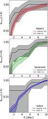 |
Fig. 6. Radial profiles, normalized to their maximum values, of the cumulative number of galaxies and AGN within a sphere of radius r < R for different protoclusters. The top, middle, and bottom panels display these profiles for galaxies (red, green, blue) and AGN (black) in MQN01, Spiderweb, and SS22, respectively. The transparent bands represent the Poissonian uncertainties in the number of objects within each sphere. The number of galaxies and AGN used to produce these curves are provided in the brackets in the legend of each panel. |
A detailed analysis using a consistent mass cutoff in the Nnorm(r < R) profiles could help clarify whether the concentration of massive galaxies toward protocluster cores is linked to the observed AGN overabundance, providing valuable insight into galaxy evolution in dense environments. However, mass estimates are currently lacking for most of the spectroscopically selected galaxies in the Spiderweb and SSA22 protoclusters. In Sect. 6.1 we nevertheless examine the impact of stellar mass on AGN activity by analyzing how stellar mass influences AGN prevalence in the limited sample of galaxies with available mass estimates.
5.3. AGN overdensity in protoclusters: An excess of the brightest AGN in MQN01
In this section we aim to quantify the AGN space density and overdensities across different luminosity ranges in MQN01 protocluster, and compare these with the same estimates in SSA22 and Spiderweb protoclusters presented in Sect. 5.1. To do it, we derived the X-ray luminosity function (XLF), which is an optimal tool to study the population of actively accreting SMBHs and to evaluate the density of such occurrences in specific parts of the Universe. To date, there is limited research on the study of AGN in high-redshift protoclusters, and more specifically, on the estimation of the XLF and the comparison with that observed in the field at the same epoch. Krishnan et al. (2017) first showed the XLF at 0.5–7 keV for the protocluster Cl 0218.3-0510 at z = 1.62 compared to that in the field. Their analysis led to the conclusion that the XLF is systematically higher in the protocluster with no clear evidence indicating discrepancies in the accretion rate distributions between AGN in the field and those within the protoclusters. Other cases are reported in recent papers such as Tozzi et al. (2022), in which the cumulative XLF in the Spiderweb protocluster and in the field are shown. This comparison shows an increase in the overdensity of AGN with 2–10 keV X-ray luminosities exceeding ∼1044 erg s−1 in Spiderweb, at each energy band. Even in Vito et al. (2024), the space density of AGN derived from the combination of two identical extreme protoclusters at z ∼ 4.3 is shown. In this study, the detection of two X-ray AGN whose L2 − 10 keV exceed 1045 erg s−1, implies an increase of three to five orders of magnitude in the XLF at the luminosity bin log(L2#x2212;10 keV/erg s−1) = 45−46 compared to the field at the same redshift.
We provide a novel comparison of the hard (2–10 keV) XLF (hereafter HXLF) of AGN estimated for a small sample of protoclusters: MQN01 (studied in this work), SSA22, and Spiderweb, and for the fields at the same redshifts. To obtain the cumulative HXLF in a grid of 2–10 keV X-ray luminosities (hereafter LX), we estimated the space density (ϕ; in Mpc−3 units) of AGN with luminosity exceeding LX, using the 1/Vmax method (Schmidt 1968; Avni & Bahcall 1980; Vito et al. 2014):
 (1)
(1)
where N(Li > LX) is the number of AGN with luminosity above LX and with spectroscopic redshift within Δz, and Ω(Li, z)≡Ω(flux), with units in steradians, represents the sky coverage shown in Fig. 2 integrated over redshift and luminosity. The range Δz corresponds to the velocity range ±Δvmax, around the redshift of the protocluster, defining the volume within which we estimated the overdensity of AGN. The term Ω(Li, z)/4π accounts for the fraction of sky covered by X-ray AGN above a given LX, and represents the area sensitive to Chandra observations above a flux threshold. We set, as maximum value of Ω a specific area (hereafter Amax) associated with the volume in which we want to estimate the overdensity of AGN in the protocluster, and this area may be particularly important for the HXLF brightest end. Breaking down the denominator of Eq. (1), we obtain the following equation:
![Mathematical equation: $$ \begin{aligned} (\mathrm{d}V/\mathrm{d}z)\mathrm{d}z = \sum _{j=1}^{n(z_{\rm bins})-1} \frac{\Omega (L,z_j)}{3} [D_{\rm comov}^3 (z_{j+1}) - D_{\rm comov}^3 (z_j)] \end{aligned} $$](/articles/aa/full_html/2025/02/aa52179-24/aa52179-24-eq23.gif) (2)
(2)
where Ω(L, zj) is multiplied by the differences between the cubic comoving distances (Dcomov) in different redshift bins. This represents the volume of a spherical shell between z and z + Δz in a specific fraction of the solid angle Ω(L, zj)/4π. To be conservative, we did not apply the incompleteness correction (see Vito et al. 2018), which was also omitted in the analysis by Tozzi et al. (2022). This correction compensates for the underestimation of the XLF at low luminosities due to the non-detection of AGN caused by sensitivity limitations. Applying this correction would only affect the values of the XLF at low luminosities, where it would increase the AGN counts. By omitting the correction, we adopt a cautious approach, ensuring that the comparison of XLFs between protoclusters remains unaffected by potential incompleteness, due to their similar sensitivity to hard X-ray flux across the fields (Fig. 2). At low luminosities, this approach provides a lower limit for the AGN overdensity in protoclusters relative to the fields. At higher luminosities, there are no effects, meaning that our primary conclusions are unaffected by this choice. The uncertainties of ϕ were estimated, by iterating the calculation in Eq. (1), randomly varying both the number of detected X-ray AGN according to the Poisson statistics, which dominate the error, and the unabsorbed luminosities, assuming a Gaussian distribution centred around the mean luminosity up to extreme values marked by the 90% confidence level values reported in Table 3.
The values of ϕ depend on the volume defined by Amax and Δvmax, as discussed above. The selection of this volume for each protocluster is critical for making appropriate comparisons of AGN densities within a given galaxy overdensity. However, as discussed in Sect. 5.1, these protoclusters lack uniformly extensive spectroscopic coverage and employ varying methods for selecting galaxy populations. This disparity impacts both the maximum areas surveyed for AGN identification and the respective completeness, thereby affecting the perceived overdensity of the AGN populations. Thus, our primary objective was to determine whether the values of ϕ and the AGN overdensities observed in MQN01, across different LX, are also present in the Spiderweb and SSA22 protoclusters, regardless of their geometrical and volumetric differences.
To achieve this, we defined the maximum volume as the one previously used in Sect. 5.2, encompassing the majority of galaxies in MQN01. Specifically, this volume has a cross-sectional area of Amax = 16 cMpc2, corresponding to the area of the MUSE mosaic, and a velocity range of Δvmax = 1000 km s−1 (see Fig. 5). This volume will be referred to as V16 hereafter. To ensure consistency with the usual methods used in literature (e.g. Tozzi et al. 2022) to estimate the HXLF, V16 was centred on the positions of the most luminous QSOs in the MQN01 and Spiderweb protoclusters, specifically CTS G18.01 (ID1) and PSK1138, respectively. These QSOs were excluded from the calculation. For the SSA22 protocluster, given the lack of a brightest QSO, V16 was centred at the location that maximizes the AGN density, following the approach used in Sect. 5.2. Thus, although V16 covers a smaller fraction of the total extent of the Spiderweb and SSA22 protoclusters, it is centred on their core regions, which are expected to correspond to the areas with the highest AGN density within these structures. Furthermore, to derive the HXLF in Spiderweb we assumed that the absorbed luminosity in the two Compton-Thick cases is ∼10% of their intrinsic luminosity, as done in Tozzi et al. (2022). For SSA22, we used the 2–8 keV X-ray luminosities reported in Lehmer et al. (2009) and multiplied by a factor of approximately 1.18 to convert these to 2–10 keV X-ray luminosities. This conversion factor was determined by modelling a power-law spectrum with a photon index of Γ = 1.8 and calculating the flux ratio between the 2–10 keV and 2–8 keV energy bands.
Figure 7 depicts the ϕ16(L > LX) derived, in V16, in the MQN01 (red line), SSA22 (blue) and Spiderweb (green) protoclusters across a range of LX of the AGN. The shaded regions represent Poissonian uncertainties, dominated mainly by Poissonian errors on the number of AGN. Dashed lines of different colours indicate the AGN cumulative HXLF in the field, as estimated by Gilli et al. (2007), at the same redshifts as the solid lines for the protoclusters. These HXLF are consistent with those derived in other studies (e.g. Ueda et al. 2014; Vito et al. 2014, 2018; Georgakakis et al. 2015; Ranalli et al. 2016; Wolf et al. 2021).
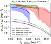 |
Fig. 7. Cumulative HXLF of AGN in a volume (V16) defined to contain the bulk of the galaxy population in MQN01, with Amax ∼ 16 cMpc2 and Δvmax = ± 1000 km s−1. The red and green lines represent the HXLF estimated for the MQN01 and Spiderweb protoclusters, respectively, centred on the brightest QSOs, CTS G18.01 (ID1) and PSK1138, which are excluded from the analysis. The blue line depicts the HXLF of AGN in the SSA22 protocluster, centred at the location that maximizes the AGN overdensity within V16. The transparent bands indicate the range of values due to Poisson uncertainties. The dashed lines indicate the HXLF of AGN in the field, estimated as in Gilli et al. (2007), with the colours corresponding to the same redshifts as the solid lines for the protoclusters. |
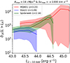 |
Fig. 8. Cumulative luminosity function of the overdensity of X-ray AGN derived as the ratio of the ϕ16 shown in Fig. 7 to the ϕ derived for the Field according to Gilli et al. (2007), normalized by the latter. The red, blue, and green curves represent the overdensities for MQN01, SSA22, and Spiderweb, respectively. |
To estimate the overdensity of AGN within V16 (hereafter δ16) in protoclusters at different redshifts, as a function of the X-ray luminosity, we adopted the following formula:
 (3)
(3)
where  is the AGN space densities obtained from Eq. (1) and ϕ(L > LX)Field is that shown in Fig. 7 as derived in Gilli et al. (2007). Figure 8 illustrates these δ16 estimates for the AGN in the MQN01 (red), SSA22 (blue), and Spiderweb (green) protoclusters.
The HXLF of the AGN population in protoclusters, at least within the volume V16, consistently exceeds that observed in the field, aligning with findings from previous studies (Krishnan et al. 2017; Tozzi et al. 2022; Vito et al. 2024) and reinforcing the elevated incidence of AGN activity in these overdense environments. Additionally, the average curves for MQN01 and Spiderweb, shown as solid lines, exhibit flatter slopes compared to those observed in the field at similar redshifts. To quantify how the slope of the HXLFs in protoclusters differ from those in fields at similar redshifts, we performed linear fits to the logarithm of ϕ16(L > LX). For MQN01 and Spiderweb, we limited the analysis to log(L2#x2212;10 keV/erg s−1) > 44 to avoid biases from incomplete corrections at lower luminosities. We then calculated the flatness score as 1 − |Sproto/(Sfield + Sproto)|, where Sproto and Sfield are the slopes of the protocluster and field HXLFs obtained from linear fits. Higher flatness scores indicate a flatter protocluster XLF, with values ranging from 0 for steep slopes to 1 for perfectly flat ones, thus reflecting the relative flatness of the protocluster XLF. The results show that MQN01 and Spiderweb exhibit flatter XLFs than their respective fields, with flatness scores of 0.62 and 0.65. Conversely, SSA22 has a steeper XLF, with a flatness score of 0.39. On average, the protoclusters exhibit slightly flatter XLFs than the fields, with a mean flatness score of 0.55. This trend is further illustrated in Fig. 8, showing the increase in δ16 with LX. In Spiderweb, the rise is particularly pronounced up to log(L2#x2212;10 keV/erg s−1) ≈ 44.4, while in MQN01, it extends up to log(L2#x2212;10 keV/erg s−1) ≈ 45.3, albeit with reduced statistical significance due to Poissonian errors. As quantified, this trend does not appear in SSA22, where no X-ray AGN are found with log(L2#x2212;10 keV/erg s−1) > 44. This discrepancy likely reflects SSA22’s distinct structure, which consists of an AGN population in extended, dense filaments rather than a central, massive node as seen in MQN01 and the Spiderweb, which are both centred on luminous massive QSOs. The overdensity of X-ray AGN in MQN01 of δ16 ∼ 102 − 104 at log(LX/erg s−1) > 45 obtained assuming a volume V16, aligns with δ in the range of three to five orders of magnitude at the luminosity bin log(L2#x2212;10 keV/erg s−1) = 45−46 found for two z ∼ 4.3 protoclusters in Vito et al. (2024). This significant overdensity in MQN01 underscores the rarity of discovering two extremely luminous AGN within approximately ∼1.5 cMpc of each other, making the type 2 AGN, ID2, particularly noteworthy. This provides clear evidence of a significant increase in the brightness of the AGN XLF in protoclusters.
As will be discussed in Sect. 6.1, the high AGN overdensity δ16 in the MQN01 protocluster could be not directly related to the protocluster environment’s effect on promoting SMBH growth. It may be a consequence of an equally high density of galaxies, highlighting the importance of estimating an AGN fraction. However, when comparing the result δ16(AGN) > 103 with the galaxy overdensity δ16(Galaxy)≃53 within the same volume4, as reported in the upcoming paper Galbiati et al. (2024), it becomes evident that the AGN overdensity cannot be solely attributed to a large density of galaxies.
6. Protocluster environments and their role in SMBH and galaxy evolution
In this section we study the relation between the properties of the detected X-ray AGN in MQN01 and the associated galaxy population in order to understand the possible effect of the environment on AGN triggering and SMBH growth. In particular, we focused on the AGN fraction as a function of galaxy stellar mass (M*) and on the SMBH accretion rate (λsBHAR). The value of these two parameters obtained for the MNQ01 field is compared to other protoclusters, such as SSA22 and Spiderweb, and to the field.
6.1. AGN fraction in MQN01: Ubiquity of accreting SMBHs in massive galaxies
One of the most straightforward parameters that can help us understand the impact of the protocluster environment on promoting SMBH growth is the fraction of galaxies within a given population that host X-ray AGN, denoted as fAGN. However, comparing fAGN across different protocluster fields is challenging due to variations in galaxy survey selection techniques and their associated completeness. Both galaxy and AGN selections are influenced by parameters such as stellar mass (M*), star formation rate (SFR), and AGN X-ray luminosity. Additionally, different methods for determining stellar masses and SFRs result in rather heterogeneous samples of galaxies as a function of M* and SFR across various fields. Consequently, the fAGN values reported in the literature for different protoclusters (Tozzi et al. 2022; Vito et al. 2023, 2024) are not easily comparable. Nonetheless, these values, typically around or above 10−2, are significantly higher than those measured in the field (< 10−2Martini et al. 2013). To illustrate how a single parameter can affect fAGN, we defined fAGN as a function of the stellar mass cut ( ) of the galaxy sample used to estimate it.
To address these challenges, we limited our analysis to the MQN01 and Spiderweb fields, as SSA22 lacks a comparable sample of M* for its galaxy population, with Monson et al. (2023) only reporting M* values for X-ray AGN. Specifically, for Spiderweb, we used values from Shimakawa et al. (2024), Pérez-Martínez et al. (2023), and an ongoing study by Pannella et al. (in prep.), each of which considers different samples obtained with different methodologies. While M* is generally well constrained through Spectral Energy Distribution (SED) fitting, the estimation of SFR is more complex, given its dependence on recent star formation history, dust extinction, and the age of the stellar population. Shimakawa et al. (2024) performed SED fitting using the X-CIGALE tool (Yang et al. 2020) with photometric data from X-ray to sub-millimetre for a sample of 84 HAEs based on narrow-band samples and BzKs colour selection (Daddi et al. 2005; Shimakawa et al. 2018). For a sample of spectroscopically selected protocluster members, using K-band Multi-Object Spectrograph (KMOS) data, Pérez-Martínez et al. (2023) applied a similar SED-fitting procedure for M* derivation, while the SFR was derived using the Kennicutt (1998) formula modified for a Chabrier (2003) IMF. They showed that SFR values from SED-fitting align with those from H α emission lines. Finally, Pannella et al. (in prep.) uses the multi-band catalog described in Tozzi et al. (2022) to estimate stellar masses through SED fitting (fastpp tool5 in Kriek et al. 2009) and SFRs by correcting the observed FUV rest-frame emission according to Eq. (10) in Pannella et al. (2015) (i.e. the correlation between UV dust attenuation and galaxy stellar mass).
Galaxies in MQN01 have been selected as discussed in Sect. 3.1.1 using the deep available MUSE data providing a complete census of galaxies with spectroscopic data above a given rest-frame UV magnitude of 26.5 (at the rest-frame reference wavelength of 150 nm). As such, they represent a population of not heavily dust-obscured star-forming galaxies. We note however, that the deep ALMA observations of Pensabene et al. (2024) did not reveal additional massive and dusty galaxies in the field with the exception of a source located at about 1″ from the QSO which is not present in either the MUSE or the Chandra sample due to the large QSO PSF in both datasets. The M* and SFR values of all the MQN01 protocluster members (listed in Table 5) have been estimated as described in Sect. 3.1.2 (see Galbiati et al. 2024, for further details).
Properties of the AGN host-galaxies derived from the SED-fitting analysis in Galbiati et al. (2024).
The top panels of Fig. 9 present the SFR versus M* distribution for galaxies in the Spiderweb protocluster (green) as obtained by Shimakawa et al. (2024) (left panel), Pérez-Martínez et al. (2023) (middle panel), and Pannella et al. (in prep.) (right panel), along with those in the MQN01 protocluster (red). The shaded areas indicate the Popesso et al. (2023) main sequence (MS) with a ±0.3 dex spread at redshifts z = 3.25 (red) and z = 2.16 (green). Galaxies hosting an X-ray AGN are marked with black-edged dots. In this analysis, we excluded the most luminous QSOs around which the protoclusters are centred, namely CTS G18.01 and the radio galaxy PSK1138, as they could represent outliers in the overall AGN and galaxy population. By comparing the positions of the Spiderweb galaxies across these three plots, the impact of galaxy selection and SFR estimation method on the evaluation of the galaxy population in the main sequence becomes evident.
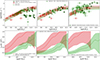 |
Fig. 9. X-ray AGN fraction versus M* threshold for different star-forming galaxy populations. The top panels display the SFR vs M* plots for galaxies in the MQN01 (red dots) and Spiderweb (green dots) regions. The Spiderweb data were obtained by Shimakawa et al. (2024) (left panel), Pérez-Martínez et al. (2023) (middle panel), and Pannella et al. (in prep.) (right panel). The shaded areas represent the Popesso et al. (2023) main sequence (MS) with a ±0.3 dex spread at redshifts z = 3.25 (red) and z = 2.16 (green). Galaxies hosting an X-ray AGN are highlighted with black-edged squares. The bottom panels show the variation of fAGN as a function of the M* threshold, as indicated by the grid of values on the x-axis. |
The bottom panels of Fig. 9 display fAGN for all samples, calculated by including galaxies with M* above the thresholds indicated on the x-axis (i.e. M*cut). To estimate the 68% binomial error for fAGN, we employed Jeffrey’s Bayesian statistics using the Python tool statsmodels. The resulting uncertainties are represented by shaded areas (for further details, see Vito et al. 2024).
As the first evidence, we found that the AGN fraction in MQN01, across all mass cuts, exceeds 0.2, placing it within the typical range of AGN fractions observed in the centre of high-redshift protoclusters (e.g. Tozzi et al. 2022; Vito et al. 2023), and thus higher than those typically observed in low-redshift galaxy clusters (fAGN < 0.02; Martini et al. 2013). On the other hand, the evidence of a wide range of fAGN observed as a function of the M*cut emphasizes the need for consistent fAGN estimation across all protoclusters to enable direct comparisons. Despite these challenges, some clear patterns are present. In all cases, fAGN increases with  , consistent with robust findings in the literature (e.g. Kauffmann et al. 2003; Best et al. 2005; Haggard et al. 2010), which show that AGN, with LX ≳ 1043.5 erg s−1, are more frequently hosted by more massive galaxies. Recently, this trend has been extended to high-redshift (2 < z < 4) AGN in dense environments identified through methods beyond just X-ray selection, as shown by Shah et al. (2024). Specifically, they demonstrate that the AGN fraction rises in higher-density regions and with increasing M*. We note that the fAGN in MQN01 is larger than that observed in Spiderweb at all masses, regardless of the details of the M* determinations. Additionally, in the MQN01 protocluster, the average fAGN (solid line) reaches 1 for galaxies with log(M∗/M⊙) > 10.5. In contrast, in Spiderweb, fAGN increases more gradually and reaches an average fAGN = 1 at log(M/M⊙) > 11.5 only using stellar masses as in Shimakawa et al. (2024), while fAGN in Spiderweb is always less than 1 with the other two methods. In other words, while Spiderweb contains massive galaxies without X-ray AGN counterparts, all galaxies in MQN01 exceeding log(M∗/M⊙) = 10.5 and selected as discussed in Sect. 3.1.1 are observed to host X-ray AGN. On the other hand, the limited sample size in this study introduces substantial uncertainties, particularly in the estimates of fAGN at higher
  , which restricts our ability to fully interpret the impact of environments characterized by high gas and galaxy densities on the correlations between their properties and nuclear activity. However, assuming that both protoclusters have nearly complete selections of massive star-forming galaxies, the observations of a larger fAGN at all the masses, and that all galaxies above a certain mass host AGN in MQN01, but not in Spiderweb, could indicate an evolutionary trend in the corresponding growth of galaxies and their SMBHs. Specifically, this evidence suggests that the MQN01 protocluster at z > 3 may have more gas available around and within galaxies for BH growth (Borisova et al. 2016; Cantalupo et al., in prep.) and/or more efficient mechanisms for triggering SMBH accretion compared to the evolutionary stage and configuration of the Spiderweb protocluster. We also performed a similar analysis, focusing exclusively on star-forming galaxies, defined as those within ±0.3 dex of the Main Sequence (MS) as characterized by Popesso et al. (2023), thus excluding points outside the MS in the SFR versus M* plots in Fig. 9. This approach allows a comparative assessment of fAGN(M* > M*cut) between the MQN01 and Spiderweb star-forming galaxy populations. The results and conclusions from this analysis are largely unchanged.
6.2. Impact of the environment on the SMBH accretion rates
To provide a rough estimate of the growth rate of individual SMBHs in the populations of the MQN01, SSA22, and Spiderweb protoclusters, we estimated the specific SMBH accretion rate parameter (λsBHAR), following the methodology described in Bongiorno et al. (2012) and Aird et al. (2018):
 (4)
(4)
where LX represents the 2–10 keV hard X-ray luminosity in erg/s, kbol is the bolometric correction factor to convert LX to the bolometric luminosity Lbol, and M* is the stellar mass of the galaxy in M⊙. Although kbol can vary as a function of both Lbol and LX (Marconi et al. 2004; Bongiorno et al. 2016; Duras et al. 2020), we adopted an average value kbol = 25, as used in Aird et al. (2018), because the uncertainties are primarily driven by other systematic errors, such as the assumption that MBH is equal to 0.002 × M* according to the relationship found by Häring & Rix (2004).
We used the LX and M* values derived in the previous section for MQN01 and Spiderweb (with the M* estimates taken from Shimakawa et al. 2024), while the M* values for AGN host galaxies in SSA22 were taken from Monson et al. (2023). We derived λsBHAR for the available sample of X-ray AGN in each protocluster, excluding the luminous QSO CTS G18.01 in the MQN01 field and the radio galaxy PSK1138 in Spiderweb. To obtain the probability density function (PDF) of λsBHAR for the SMBH populations in these different environments, we adopted the non-parametric Kernel Density Estimation (KDE) method (see Moon et al. 1995, and references therein). The PDF of λsBHAR for SMBH populations in MQN01 (red), SSA22 (blue), and Spiderweb (green) are depicted as dashed lines in Fig. 10.
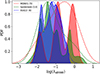 |
Fig. 10. Probability density function (PDF) of the λsBHAR parameter for the three SMBH populations hosted in the MQN01 (red), SSA22 (blue) and Spiderweb (green) protoclusters. The solid lines represent the λsBHAR PDFs obtained using an iterative procedure that incorporates additional artificial sources, created by randomly varying LX and M* within their 1σ uncertainties. The dashed lines show the λsBHAR PDFs without applying this iterative procedure, with the number of AGN indicated in brackets in the legend. |
To enhance statistical robustness and better characterize the λsBHAR distribution and properties of individual AGN while accounting for measurement uncertainties, we employed an iterative approach using a bootstrap algorithm. This method involves expanding the initial sample by adding sources with λsBHAR values derived from randomly varying the parameters LX and M* within their respective 1σ uncertainties. This process effectively increases the sample size and provides a more comprehensive representation of the underlying distribution. The resulting λsBHAR PDFs are shown in Fig. 10 as solid lines subtended by coloured areas.
The comparison of the peaks in the λsBHAR PDFs represented by dashed lines, which can be considered as average estimates, suggests that MQN01 has a higher fraction of rapidly accreting SMBHs compared to the other protoclusters. How does this result compare to findings at different redshifts in different environments? Using deep X-ray observations from the XMM Large Scale Structure (XMM-LSS), COSMOS, and European Large-Area ISO Survey (ELAIS-S1) extragalactic fields, Aird et al. (2012) found that the probability for a galaxy to host an AGN with a given λsBHAR (p(log(λsBHAR)|M*, z)) follows a power-law distribution. This distribution is truncated at the Eddington limit, likely due to the self-regulation of SMBH growth (Aird et al. 2012, 2018; Bongiorno et al. 2012). In a more recent study, Aird et al. (2018) observed an evolution of the p(log(λsBHAR)|M*, z) for star-forming galaxies with M∗ > 1010 M⊙, noting that λsBHAR shifts toward higher values at higher redshifts. This shift significantly impacts the increasing AGN duty cycle, defined as the fraction of galaxies with log(λsBHAR) > 0.1. This trend could be explained by the greater access to a larger reservoir of cold gas for galaxies at higher redshifts. The average values of λsBHAR found for galaxies in protoclusters (i.e. the peaks of dashed lines in Fig. 10) align with the cosmic evolution of the average accretion rate (log⟨λsBHAR⟩) as presented by Aird et al. (2018). Specifically, they obtained λsBHAR distributions in the field that peaks around log⟨λsBHAR⟩≈ − 1 for star-forming galaxies at z > 2 and log⟨λsBHAR⟩≈ − 0.5 at z > 3. Thus, the average λsBHAR distribution of AGN in protoclusters does not show significant deviation from the larger AGN sample in Aird et al. (2018). However, this comparison should be taken with caution as it could be affected by several factors, such as the broad distribution of λsBHAR values observed, the limited sample size, AGN activity variability, the uncertainties in λsBHAR measurements, and different methods in the selection of the galaxy populations, as well as the determination of M* and SFR.
The PDFs of λsBHAR, indicated by solid lines, reveal groups of AGN with specific λsBHAR values. In the MQN01 and Spiderweb protoclusters, some AGN are found with λsBHAR values near the Eddington limit. The presence of these AGN could indicate that, within the same overdensity, different galaxies could be subject to different environmental (e.g. varying amounts of surrounding gas and galaxies) and non-environmental (e.g. different internal gas transport mechanisms, accretion disc instabilities, feedback cycles) factors leading them to experience different accretion phases. In Fig. 11 we explore whether such differences in λsBHAR across AGN in MQN01 and Spiderweb could depend on the projected distance from the centre of the protocluster (defined as the position of the central QSO in MQN01 and PKS 1138-262 in Spiderweb). The black dots represent the median λsBHAR values, with error bars indicating the 16th and 84th percentiles, for AGN in both protoclusters across different radial bins from the main QSOs. Despite the limited sample size, both Pearson and Spearman correlation analyses indicate a strong and statistically significant negative relationship between λsBHAR and the distance from the protocluster centre in Spiderweb and MQN01 (i.e. black dots). The Pearson correlation shows a mean value of –0.71 with a 95% confidence interval of [–0.90, –0.52], while the Spearman correlation is slightly stronger, with a mean value of –0.76 and a 95% confidence interval of [–0.83, –0.60]. These results suggest that SMBH accretion rates are higher in the central, denser regions of protoclusters.
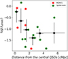 |
Fig. 11. λsBHAR as a function of the distance from the central QSOs, CTS G18.01 in MQN01 (red) and PSK1138 in the Spiderweb (green) protocluster. The black dots mark the median values of λsBHAR for the AGN in both protoclusters across different bins of distance from the two central QSOs. The uncertainties correspond to the 16th and 84th percentile values within each radial bin. |
7. Connecting AGN populations to large-scale structure in protoclusters
In the context of protoclusters, AGN activity is often influenced by environmental factors such as the density of gas and galaxies, galaxy mergers, and gas accretion along cosmic filaments. High-density regions, like those in protoclusters, tend to favour higher rates of galaxy interactions and mergers, which can trigger or enhance AGN activity (e.g. Sijacki et al. 2007; Menci et al. 2008). Moreover, the accretion of gas along large-scale structures, such as the cosmic filaments traced by Ly α nebulae, has been suggested to modulate AGN luminosities and accretion rates (e.g. Silk 2005; Bower et al. 2017).
In Sects. 5 and 6, we presented analyses comparing the collective properties of AGN in MQN01 with those in the SSA22 and Spiderweb protoclusters. While limitations arising from differences in study methodologies, sample sizes, and data uncertainties hinder direct comparisons, these analyses provide a solid foundation for exploring potential connections between the properties of these three distinct large-scale structures and their AGN populations. Our results indicate that the AGN population in SSA22 is weaker in luminosity, less centrally concentrated, and exhibits slower SMBH accretion rates compared to those in MQN01 and Spiderweb. We speculate that this difference could be linked to the structural characteristics of SSA22, which lacks a super-luminous AGN marking a clear centre. Both the distribution of galaxies within SSA22 and the morphology of its Ly α nebula, as shown by Umehata et al. (2019), suggest that this overdensity primarily traces an association of dense but non-converging filaments rather than a “node”, a high-density region where multiple filaments converge. The filamentary structure in SSA22 may eventually evolve into a more compact, dense core, potentially forming a “node” in the future. In contrast, the comparison of AGN properties between MQN01 and Spiderweb reveals fewer differences. This similarity likely reflects the more compact gas and galaxy configurations in both protoclusters, which are less extended than in SSA22. The extended Ly α nebula in Spiderweb (Miley et al. 2006), as well as in MQN01 (see Borisova et al. 2016), exhibit a morphology closer to circular symmetry, in contrast to the more irregular structure observed in SSA22. Therefore, we propose that the primary distinction between these protoclusters lies in the different evolutionary stages at which they are observed (more advanced in MQN01 and Spiderweb, compared to SSA22), with redshift being a secondary factor likely exerting a less direct influence on the AGN/galaxy populations.
Interestingly, massive galaxies in MQN01 are more likely to host an AGN compared to Spiderweb (see Fig. 9), which could provide insight into SMBH-galaxy co-evolution in these environments. However, the current sample size and available data do not allow for a more detailed exploration of this co-evolution. Future observations and more detailed data will be needed to further investigate how the environment shapes this relationship, particularly in high-redshift protoclusters. Although more robust insight will be gained through future analyses, even with the current data, we can already discern how distinct large-scale structural features influence AGN populations, underscoring the connection between nuclear activity (small scales) and the cosmic web (large scales). Future detailed analyses will further elucidate the feeding and feedback processes shaping these interactions. In summary, the comparison between the protoclusters in this study suggests that environmental factors might shape AGN populations differently, depending on the morphology and compactness of the filamentary structures within these regions.
8. Summary and conclusions
We presented the analysis of deep (∼634 ks) Chandra observations in a field known as MQN01 centred on a luminous QSO at z ∼ 3.2502. The field contains a giant Ly α nebula (Borisova et al. 2016; Cantalupo et al., in prep.) and one of the largest overdensities of UV continuum selected galaxies found to date at this redshift (Galbiati et al. 2024; Pensabene et al. 2024). The deep Chandra observations were used to obtain a comprehensive census of AGN embedded into this protocluster and to derive the hard X-ray luminosity function (HXLF), the overdensity (δ), the fraction of AGN (fAGN), and the accretion rates of the SMBHs (λsBHAR) in this field. These quantities have been compared to similar properties obtained for the other two protoclusters available in the literature with deep Chandra observations, Spiderweb (Tozzi et al. 2022), and SSA22 (Lehmer et al. 2009). The key findings are summarized below:
-
We have identified six X-ray AGN with log(L2#x2212;10 keV/erg s−1) ≳ 43.5 among the spectroscopically selected protocluster members within an area of ≈16 cMpc2 (≈2 × 2 arcmin2) and a velocity range of ±1000 km s−1 around the most luminous QSO. The AGN overdensity above the survey luminosity within this volume, excluding the QSO, corresponds to ⟨δ16⟩≃103. This is one of the largest AGN overdensities found so far at z > 2, exceeding, on average, the overdensities calculated within similar volumes and luminosities within the Spiderweb field (⟨δ16⟩≃600) and SSA22 (⟨δ16⟩≃400) as shown in Fig. 8. Moreover, the AGN HXLF in MQN01, similarly to the Spiderweb, is much flatter compared to those observed in the field at the same redshift for log(L2#x2212;10 keV/erg s−1) > 44.5, showing an even higher overdensity of high-luminosity AGN compared to the field above these luminosities.
-
The total fraction of AGN above the survey luminosity derived in MQN01 (fAGN > 0.2) exceeds those calculated in low-redshift galaxy clusters and in the field (fAGN < 0.02), and is comparable to those estimated in other protoclusters (Tozzi et al. 2022; Vito et al. 2023). The fAGN in the MQN01, similarly to the Spiderweb, increases substantially considering galaxies of higher stellar mass, as shown in Fig. 9. Surprisingly, the four most massive galaxies spectroscopically selected with MUSE in the MQN01 exceeding log(M∗/M⊙) > 10.5 are all AGN. This is different to what is observed in the Spiderweb field for which fAGN remains around or below 50% above these masses considering three different selection techniques. However, we caution that this result is sensitive to the low statistics and the particular selection technique in the MQN01 field.
-
The λsBHAR PDFs indicate that MQN01 hosts a higher fraction of rapidly accreting SMBHs compared to SSA22 and Spiderweb. Some AGN in MQN01 and Spiderweb approach the Eddington limit. A wide distribution of λsBHAR of about 2 dex within the same overdensity suggests variations in galaxy accretion phases and surrounding gas availability can significantly influence SMBH growth. The λsBHAR increases with proximity to the central QSOs in the MQN01 and Spiderweb protoclusters, suggesting that denser environments could indeed enhance SMBH accretion rates.
In conclusion, our results suggest that protocluster environments such as the one probed by the MQN01 field host physical conditions that are ideal to promote the triggering and growth of X-ray AGN, especially for galaxies with stellar masses above log(M∗/M⊙) = 10.5. This configuration represents a rare occurrence for an AGN population, and it is even more exceptional considering the variability in X-ray luminosity during the AGN phase. However, as suggested in the literature by simulations (see Di Matteo et al. 2005; Jiang & Dai 2024), the high-density regions, especially those with large gas reservoirs at these redshifts (e.g. Zou et al. 2024), may play a crucial role in prolonging the period during which an SMBH can sustain rapid accretion. In the second part of this project, we focused on the individual properties of AGN host galaxies within the MQN01 protocluster, examining them within the broader context of co-evolving SMBHs and large-scale structures.
In the analyses presented in this paper, Poissonian uncertainties provide a challenge for the determination of the role of environmental factors and galaxy properties on SMBH accretion and growth. To draw more definitive conclusions, future studies will need to perform homogeneous observations across multiple wavelengths in diverse protocluster fields, covering a broad range of redshifts and overdensities. Therefore, further deep X-ray surveys of protoclusters are essential to expand these studies. X-ray missions with greatly increased sensitivity and fields of view, such as Athena (Nandra et al. 2013) and Lynx (Gaskin et al. 2019), would overcome the limited statistics and allow the extension of these studies to many more protoclusters and to higher redshifts.
For the X-ray fit parameters, we used a commonly adopted confidence level of 90%.
Corresponding to the wavelet scales 1.0 1.414 2.0 2.828 4.0 5.657 8.0 11.314 16.0.
δ16 = 53 ± 17.4 at MR ≤ −19.25 mag.
Acknowledgments
This project was supported by the European Research Council (ERC) Consolidator Grant 864361 (CosmicWeb). FF acknowledges supported by HORIZON2020: AHEAD2020-Grant Agreement n. 871158. PT acknowledges support from the Next Generation European Union PRIN 2022 20225E4SY5 – “From ProtoClusters to Clusters in one Gyr”. This work is based on observations collected with the X-ray Chandra telescope (proposal number 23700358, Cycle 23), and at the European Southern Observatory under ESO programs IDs 102.A-0448(A) and 110.23ZX. This work made use of Astropy (http://www.astropy.org) a community-developed core Python package and ecosystem of tools and resources for astronomy (Astropy Collaboration 2013, 2018), as well as Numpy (Harris et al. 2020), SciPy (Virtanen et al. 2020), and Matplotlib (Hunter 2007).
References
- Aird, J., Coil, A. L., Moustakas, J., et al. 2012, ApJ, 746, 90 [CrossRef] [Google Scholar]
- Aird, J., Coil, A. L., Georgakakis, A., et al. 2015, MNRAS, 451, 1892 [Google Scholar]
- Aird, J., Coil, A. L., & Georgakakis, A. 2018, MNRAS, 474, 1225 [NASA ADS] [CrossRef] [Google Scholar]
- Andreon, S., Romero, C., Aussel, H., et al. 2023, MNRAS, 522, 4301 [NASA ADS] [CrossRef] [Google Scholar]
- Arnaud, K. A. 1996, in Astronomical Data Analysis Software and Systems V, eds. G. H. Jacoby, & J. Barnes, Astronomical Society of the Pacific Conference Series, 101, 17 [NASA ADS] [Google Scholar]
- Arrigoni Battaia, F., Prochaska, J. X., Hennawi, J. F., et al. 2018, MNRAS, 473, 3907 [NASA ADS] [CrossRef] [Google Scholar]
- Assef, R. J., Eisenhardt, P. R. M., Stern, D., et al. 2015, ApJ, 804, 27 [Google Scholar]
- Astropy Collaboration (Robitaille, T. P., et al.) 2013, A&A, 558, A33 [NASA ADS] [CrossRef] [EDP Sciences] [Google Scholar]
- Astropy Collaboration (Price-Whelan, A. M., et al.) 2018, AJ, 156, 123 [Google Scholar]
- Avni, Y., & Bahcall, J. N. 1980, ApJ, 235, 694 [NASA ADS] [CrossRef] [Google Scholar]
- Best, P. N., Kauffmann, G., Heckman, T. M., & Ivezić, Ž. 2005, MNRAS, 362, 9 [Google Scholar]
- Binney, J., & Tabor, G. 1995, MNRAS, 276, 663 [NASA ADS] [Google Scholar]
- Bongiorno, A., Merloni, A., Brusa, M., et al. 2012, MNRAS, 427, 3103 [Google Scholar]
- Bongiorno, A., Schulze, A., Merloni, A., et al. 2016, A&A, 588, A78 [NASA ADS] [CrossRef] [EDP Sciences] [Google Scholar]
- Borisova, E., Cantalupo, S., Lilly, S. J., et al. 2016, ApJ, 831, 39 [Google Scholar]
- Bower, R. G., Schaye, J., Frenk, C. S., et al. 2017, MNRAS, 465, 32 [NASA ADS] [CrossRef] [Google Scholar]
- Boyle, B. J., Georgantopoulos, I., Blair, A. J., et al. 1998, MNRAS, 296, 1 [NASA ADS] [CrossRef] [Google Scholar]
- Bruzual, G., & Charlot, S. 2003, MNRAS, 344, 1000 [NASA ADS] [CrossRef] [Google Scholar]
- Calzetti, D., Armus, L., Bohlin, R. C., et al. 2000, ApJ, 533, 682 [NASA ADS] [CrossRef] [Google Scholar]
- Cantalupo, S., Arrigoni-Battaia, F., Prochaska, J. X., Hennawi, J. F., & Madau, P. 2014, Nature, 506, 63 [Google Scholar]
- Carilli, C. L., Röttgering, H. J. A., van Ojik, R., Miley, G. K., & van Breugel, W. J. M. 1997, ApJS, 109, 1 [NASA ADS] [CrossRef] [Google Scholar]
- Carraro, R., Rodighiero, G., Cassata, P., et al. 2020, A&A, 642, A65 [EDP Sciences] [Google Scholar]
- Chabrier, G. 2003, PASP, 115, 763 [Google Scholar]
- Champagne, J. B., Casey, C. M., Zavala, J. A., et al. 2021, ApJ, 913, 110 [NASA ADS] [CrossRef] [Google Scholar]
- Cicone, C., Maiolino, R., Gallerani, S., et al. 2015, A&A, 574, A14 [NASA ADS] [CrossRef] [EDP Sciences] [Google Scholar]
- Cowie, L. L., Gardner, J. P., Hu, E. M., et al. 1994, ApJ, 434, 114 [NASA ADS] [CrossRef] [Google Scholar]
- Croft, S., Kurk, J., van Breugel, W., et al. 2005, AJ, 130, 867 [NASA ADS] [CrossRef] [Google Scholar]
- Cucciati, O., Zamorani, G., Lemaux, B. C., et al. 2014, A&A, 570, A16 [NASA ADS] [CrossRef] [EDP Sciences] [Google Scholar]
- da Costa, M. R., & Menéndez-Delmestre, K. 2021, Astron. Nachr., 342, 153 [CrossRef] [Google Scholar]
- Daddi, E., Dickinson, M., Giavalisco, M., et al. 2005, BzK selected starburst galaxies at z = 2 in GOODS-S: masses, star- formation rates and stellar populations, 381 [Google Scholar]
- Dannerbauer, H., Kurk, J. D., De Breuck, C., et al. 2014, VizieR On-line Data Catalog: J/A+A/570/A55 [Google Scholar]
- Digby-North, J. A., Nandra, K., Laird, E. S., et al. 2010, MNRAS, 407, 846 [NASA ADS] [CrossRef] [Google Scholar]
- Di Mascolo, L., Saro, A., Mroczkowski, T., et al. 2023, Nature, 615, 809 [NASA ADS] [CrossRef] [Google Scholar]
- Di Matteo, T., Springel, V., & Hernquist, L. 2005, Nature, 433, 604 [NASA ADS] [CrossRef] [Google Scholar]
- Dubois, Y., Gavazzi, R., Peirani, S., & Silk, J. 2013, MNRAS, 433, 3297 [CrossRef] [Google Scholar]
- Duras, F., Bongiorno, A., Ricci, F., et al. 2020, A&A, 636, A73 [NASA ADS] [CrossRef] [EDP Sciences] [Google Scholar]
- Elford, J. S., Davis, T. A., Ruffa, I., et al. 2024, MNRAS, 528, 319 [NASA ADS] [CrossRef] [Google Scholar]
- Fabian, A. C., Sanders, J. S., Allen, S. W., et al. 2003, MNRAS, 344, L43 [NASA ADS] [CrossRef] [Google Scholar]
- Freeman, P., Doe, S., & Siemiginowska, A. 2001, in Astronomical Data Analysis, eds. J. L. Starck, & F. D. Murtagh, Society of Photo-Optical Instrumentation Engineers (SPIE) Conference Series, 4477, 76 [Google Scholar]
- Galbiati, M., Cantalupo, S., Steidel, C., et al. 2024, A&A, submitted [arXiv:2410.03822] [Google Scholar]
- Gaskin, J. A., Swartz, D. A., Vikhlinin, A., et al. 2019, J. Astron. Telesc. Instrum. Syst., 5, 021001 [NASA ADS] [Google Scholar]
- Gehrels, N. 1986, ApJ, 303, 336 [Google Scholar]
- Georgakakis, A., Aird, J., Buchner, J., et al. 2015, MNRAS, 453, 1946 [Google Scholar]
- Giacconi, R., Rosati, P., Tozzi, P., et al. 2001, ApJ, 551, 624 [Google Scholar]
- Gilli, R., Comastri, A., & Hasinger, G. 2007, A&A, 463, 79 [NASA ADS] [CrossRef] [EDP Sciences] [Google Scholar]
- Gobat, R., Daddi, E., Onodera, M., et al. 2011, A&A, 526, A133 [NASA ADS] [CrossRef] [EDP Sciences] [Google Scholar]
- Gobat, R., Daddi, E., Coogan, R. T., et al. 2019, A&A, 629, A104 [NASA ADS] [CrossRef] [EDP Sciences] [Google Scholar]
- Haggard, D., Green, P. J., Anderson, S. F., et al. 2010, ApJ, 723, 1447 [NASA ADS] [CrossRef] [Google Scholar]
- Häring, N., & Rix, H.-W. 2004, ApJ, 604, L89 [Google Scholar]
- Harris, C. R., Millman, K. J., van der Walt, S. J., et al. 2020, Nature, 585, 357 [NASA ADS] [CrossRef] [Google Scholar]
- Harrison, C. M., & Ramos Almeida, C. 2024, Galaxies, 12, 17 [NASA ADS] [CrossRef] [Google Scholar]
- Hatch, N. A., Kurk, J. D., Pentericci, L., et al. 2011, MNRAS, 415, 2993 [NASA ADS] [CrossRef] [Google Scholar]
- Hatch, N. A., Wylezalek, D., Kurk, J. D., et al. 2014, MNRAS, 445, 280 [NASA ADS] [CrossRef] [Google Scholar]
- Hayashino, T., Matsuda, Y., Tamura, H., et al. 2004, AJ, 128, 2073 [Google Scholar]
- Hennawi, J. F., Prochaska, J. X., Cantalupo, S., & Arrigoni-Battaia, F. 2015, Science, 348, 779 [Google Scholar]
- Higuchi, R., Ouchi, M., Ono, Y., et al. 2019, ApJ, 879, 28 [Google Scholar]
- Hopkins, P. F., Somerville, R. S., Hernquist, L., et al. 2006, ApJ, 652, 864 [NASA ADS] [CrossRef] [Google Scholar]
- Hunter, J. D. 2007, CSE, 9, 90 [Google Scholar]
- Jiang, Y. F., & Dai, L. 2024, arXiv e-prints [arXiv:2408.16856] [Google Scholar]
- Jin, S., Dannerbauer, H., Emonts, B., et al. 2021, A&A, 652, A11 [NASA ADS] [CrossRef] [EDP Sciences] [Google Scholar]
- Kauffmann, G., Heckman, T. M., Tremonti, C., et al. 2003, MNRAS, 346, 1055 [Google Scholar]
- Kennicutt, R. C., Jr. 1998, ARA&A, 36, 189 [Google Scholar]
- King, A., & Nixon, C. 2015, MNRAS, 453, L46 [NASA ADS] [CrossRef] [Google Scholar]
- Kormendy, J., & Ho, L. C. 2013, ARA&A, 51, 511 [Google Scholar]
- Kriek, M., van Dokkum, P. G., Franx, M., Illingworth, G. D., & Magee, D. K. 2009, ApJ, 705, L71 [NASA ADS] [CrossRef] [Google Scholar]
- Krishnan, C., Hatch, N. A., Almaini, O., et al. 2017, MNRAS, 470, 2170 [NASA ADS] [CrossRef] [Google Scholar]
- Kubo, M., Yamada, T., Ichikawa, T., et al. 2015, ApJ, 799, 38 [NASA ADS] [CrossRef] [Google Scholar]
- Kubo, M., Yamada, T., Ichikawa, T., et al. 2016, MNRAS, 455, 3333 [CrossRef] [Google Scholar]
- Kuiper, E., Hatch, N. A., Miley, G. K., et al. 2011, MNRAS, 415, 2245 [NASA ADS] [CrossRef] [Google Scholar]
- Kurk, J. D., Röttgering, H. J. A., Pentericci, L., et al. 2000, A&A, 358, L1 [NASA ADS] [Google Scholar]
- Kurk, J. D., Pentericci, L., Overzier, R. A., Röttgering, H. J. A., & Miley, G. K. 2004a, A&A, 428, 817 [NASA ADS] [CrossRef] [EDP Sciences] [Google Scholar]
- Kurk, J. D., Pentericci, L., Röttgering, H. J. A., & Miley, G. K. 2004b, A&A, 428, 793 [NASA ADS] [CrossRef] [EDP Sciences] [Google Scholar]
- Lanzuisi, G., Civano, F., Elvis, M., et al. 2013, MNRAS, 431, 978 [NASA ADS] [CrossRef] [Google Scholar]
- Lehmer, B. D., Alexander, D. M., Chapman, S. C., et al. 2009, MNRAS, 400, 299 [Google Scholar]
- Lepore, M., Di Mascolo, L., Tozzi, P., et al. 2024, A&A, 682, A186 [NASA ADS] [CrossRef] [EDP Sciences] [Google Scholar]
- Liu, T., Tozzi, P., Wang, J.-X., et al. 2017, ApJS, 232, 8 [NASA ADS] [CrossRef] [Google Scholar]
- Luo, B., Brandt, W. N., Xue, Y. Q., et al. 2017, ApJS, 228, 2 [Google Scholar]
- Macuga, M., Martini, P., Miller, E. D., et al. 2019, ApJ, 874, 54 [NASA ADS] [CrossRef] [Google Scholar]
- Magorrian, J., Tremaine, S., Richstone, D., et al. 1998, AJ, 115, 2285 [Google Scholar]
- Marchesi, S., Mignoli, M., Gilli, R., et al. 2023, A&A, 673, A97 [NASA ADS] [CrossRef] [EDP Sciences] [Google Scholar]
- Marconi, A., Risaliti, G., Gilli, R., et al. 2004, MNRAS, 351, 169 [Google Scholar]
- Martini, P., Miller, E. D., Brodwin, M., et al. 2013, ApJ, 768, 1 [Google Scholar]
- Matsuda, Y., Yamada, T., Hayashino, T., et al. 2004, AJ, 128, 569 [NASA ADS] [CrossRef] [Google Scholar]
- Mawatari, K., Inoue, A. K., Yamada, T., et al. 2023, AJ, 165, 208 [Google Scholar]
- Menci, N., Cavaliere, A., Fontana, A., et al. 2003, ApJ, 587, L63 [NASA ADS] [CrossRef] [Google Scholar]
- Menci, N., Fiore, F., Puccetti, S., & Cavaliere, A. 2008, ApJ, 686, 219 [NASA ADS] [CrossRef] [Google Scholar]
- Miley, G., & De Breuck, C. 2008, A&ARv, 15, 67 [Google Scholar]
- Miley, G. K., Overzier, R. A., Zirm, A. W., et al. 2006, ApJ, 650, L29 [NASA ADS] [CrossRef] [Google Scholar]
- Monson, E. B., Doore, K., Eufrasio, R. T., et al. 2023, ApJ, 951, 15 [NASA ADS] [CrossRef] [Google Scholar]
- Moon, Y.-I., Rajagopalan, B., & Lall, U. 1995, Phys. Rev. E, 52, 2318 [CrossRef] [Google Scholar]
- Nandra, K., Barret, D., Barcons, X., et al. 2013, arXiv e-prints [arXiv:1306.2307] [Google Scholar]
- Overzier, R. A. 2016, A&ARv, 24, 14 [Google Scholar]
- Pannella, M., Elbaz, D., Daddi, E., et al. 2015, ApJ, 807, 141 [Google Scholar]
- Pensabene, A., Cantalupo, S., Cicone, C., et al. 2024, A&A, 684, A119 [NASA ADS] [CrossRef] [EDP Sciences] [Google Scholar]
- Pentericci, L., Roettgering, H. J. A., Miley, G. K., Carilli, C. L., & McCarthy, P. 1997, A&A, 326, 580 [Google Scholar]
- Pentericci, L., Kurk, J. D., Röttgering, H. J. A., et al. 2000, A&A, 361, L25 [NASA ADS] [Google Scholar]
- Pérez-Martínez, J. M., Dannerbauer, H., Kodama, T., et al. 2023, MNRAS, 518, 1707 [Google Scholar]
- Planck Collaboration VI. 2018, A&A, 641, A6 [Google Scholar]
- Popesso, P., Concas, A., Cresci, G., et al. 2023, MNRAS, 519, 1526 [Google Scholar]
- Ranalli, P., Koulouridis, E., Georgantopoulos, I., et al. 2016, A&A, 590, A80 [NASA ADS] [CrossRef] [EDP Sciences] [Google Scholar]
- Roettgering, H. J. A., Lacy, M., Miley, G. K., Chambers, K. C., & Saunders, R. 1994, A&AS, 108, 79 [NASA ADS] [Google Scholar]
- Rosati, P., Tozzi, P., Giacconi, R., et al. 2002, ApJ, 566, 667 [Google Scholar]
- Schawinski, K., Koss, M., Berney, S., & Sartori, L. F. 2015, MNRAS, 451, 2517 [Google Scholar]
- Schmidt, M. 1968, ApJ, 151, 393 [Google Scholar]
- Scholz, F. W., & Stephens, M. A. 1987, J. Am. Stat. Assoc., 82, 918 [Google Scholar]
- Shah, E. A., Lemaux, B. C., Forrest, B., et al. 2024, A&A, submitted [arXiv:2409.02996] [Google Scholar]
- Shimakawa, R., Kodama, T., Tadaki, K.-I., et al. 2015, MNRAS, 448, 666 [NASA ADS] [CrossRef] [Google Scholar]
- Shimakawa, R., Koyama, Y., Röttgering, H. J. A., et al. 2018, MNRAS, 481, 5630 [NASA ADS] [CrossRef] [Google Scholar]
- Shimakawa, R., Pérez-Martínez, J. M., Koyama, Y., et al. 2024, MNRAS, 528, 3679 [NASA ADS] [CrossRef] [Google Scholar]
- Sijacki, D., Springel, V., Di Matteo, T., & Hernquist, L. 2007, MNRAS, 380, 877 [NASA ADS] [CrossRef] [Google Scholar]
- Silk, J. 2005, MNRAS, 364, 1337 [NASA ADS] [CrossRef] [Google Scholar]
- Stanford, S. A., Brodwin, M., Gonzalez, A. H., et al. 2012, ApJ, 753, 164 [Google Scholar]
- Steidel, C. C., Adelberger, K. L., Dickinson, M., et al. 1998, ApJ, 492, 428 [Google Scholar]
- Steidel, C. C., Adelberger, K. L., Shapley, A. E., et al. 2000, ApJ, 532, 170 [NASA ADS] [CrossRef] [Google Scholar]
- Steidel, C. C., Bogosavljević, M., Shapley, A. E., et al. 2018, ApJ, 869, 123 [Google Scholar]
- Sturm, E., González-Alfonso, E., Veilleux, S., et al. 2011, ApJ, 733, L16 [NASA ADS] [CrossRef] [Google Scholar]
- Tadaki, K.-I., Kodama, T., Hayashi, M., et al. 2019, PASJ, 71, 40 [NASA ADS] [CrossRef] [Google Scholar]
- Tanaka, M., Toft, S., Marchesini, D., et al. 2013, ApJ, 772, 113 [NASA ADS] [CrossRef] [Google Scholar]
- Toshikawa, J., Kashikawa, N., Overzier, R., et al. 2016, ApJ, 826, 114 [NASA ADS] [CrossRef] [Google Scholar]
- Tozzi, P., Rosati, P., Nonino, M., et al. 2001, ApJ, 562, 42 [NASA ADS] [CrossRef] [Google Scholar]
- Tozzi, P., Santos, J. S., Jee, M. J., et al. 2015, ApJ, 799, 93 [Google Scholar]
- Tozzi, P., Pentericci, L., Gilli, R., et al. 2022, A&A, 662, A54 [NASA ADS] [CrossRef] [EDP Sciences] [Google Scholar]
- Travascio, A., Zappacosta, L., Cantalupo, S., et al. 2020, A&A, 635, A157 [NASA ADS] [CrossRef] [EDP Sciences] [Google Scholar]
- Tytler, D., Fan, X. M., Burles, S., et al. 1995, in QSO Absorption Lines, ed. G. Meylan, 289 [CrossRef] [Google Scholar]
- Uchiyama, H., Yamashita, T., Nagao, T., et al. 2022, ApJ, 934, 68 [NASA ADS] [CrossRef] [Google Scholar]
- Ueda, Y., Akiyama, M., Hasinger, G., Miyaji, T., & Watson, M. G. 2014, ApJ, 786, 104 [Google Scholar]
- Umehata, H., Tamura, Y., Kohno, K., et al. 2014, MNRAS, 440, 3462 [Google Scholar]
- Umehata, H., Tamura, Y., Kohno, K., et al. 2015, ApJ, 815, L8 [Google Scholar]
- Umehata, H., Fumagalli, M., Smail, I., et al. 2019, Science, 366, 97 [Google Scholar]
- van Marrewijk, J., Di Mascolo, L., Gill, A. S., et al. 2024, A&A, 689, A41 [NASA ADS] [CrossRef] [EDP Sciences] [Google Scholar]
- Virtanen, P., Gommers, R., Oliphant, T. E., et al. 2020, NatMe, 17, 261 [NASA ADS] [Google Scholar]
- Vito, F., Gilli, R., Vignali, C., et al. 2014, MNRAS, 445, 3557 [Google Scholar]
- Vito, F., Brandt, W. N., Yang, G., et al. 2018, MNRAS, 473, 2378 [Google Scholar]
- Vito, F., Brandt, W. N., Lehmer, B. D., et al. 2020, A&A, 642, A149 [NASA ADS] [CrossRef] [EDP Sciences] [Google Scholar]
- Vito, F., Tozzi, P., Gilli, R., et al. 2023, arXiv e-prints [arXiv:2311.08466] [Google Scholar]
- Vito, F., Brandt, W. N., Comastri, A., et al. 2024, A&A, 689, A130 [NASA ADS] [CrossRef] [EDP Sciences] [Google Scholar]
- Wolf, J., Nandra, K., Salvato, M., et al. 2021, A&A, 647, A5 [NASA ADS] [CrossRef] [EDP Sciences] [Google Scholar]
- Yamada, T., Matsuda, Y., Kousai, K., et al. 2012, ApJ, 751, 29 [NASA ADS] [CrossRef] [Google Scholar]
- Yang, G., Boquien, M., Buat, V., et al. 2020, MNRAS, 491, 740 [Google Scholar]
- Zou, F., Yu, Z., Brandt, W. N., et al. 2024, ApJ, 964, 183 [NASA ADS] [CrossRef] [Google Scholar]
Appendix A: Zoom-in of the count maps of the X-ray protocluster members and their spectra
In this section we report the Chandra X-ray images in the soft (0.5-2.0 keV; top panel), hard (2.0-7.0 keV; central panel), and broad (0.5-7.0 keV; bottom panel) energy bands, zoomed in on the six X-ray sources associated with spectroscopically selected protocluster members, in Fig. A.1. This image is essential for highlighting the significant number of counts in each band for the X-ray sources associated with the protocluster members. Moreover, it illustrates our ability to deblend the X-ray detections of ID3 and ID4. Specifically, ID3 is primarily visible in the hard X-ray band, while ID4 is more prominent in the soft band. This allows us to confidently determine that these two slightly blended sources are associated with two distinct MUSE-selected protocluster members. We estimated the S/N of each source in the 0.5-10 keV energy band within a 2”-radius and estimated the background in a 4”-6” annulus, by masking the contribution of close X-ray sources. Additionally, we assessed how each X-ray AGN’s S/N compares to the rest of the X-ray source catalog by determining the percentage of sources with S/N greater than that of each X-ray AGN in MQN01. For the most luminous sources, ID1 and ID2, we obtained S/N values of ≈50 (with ∼1% of the sources in the catalog having higher S/N) and 20 (with ∼5% having higher S/N), respectively. For the sources ID3, ID4, ID5 and ID6, we obtained S/N values of 5.4 (∼50%), 5.1 (∼62%), 6.4 (∼37%) and 4 (∼84%), with the corresponding percentages of catalog sources having higher S/N.
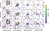 |
Fig. A.1. Chandra X-ray images (in counts) focusing on the six X-ray sources associated with spectroscopically selected protocluster members. The images are binned in energy bands: soft (0.5-2.0 keV) in the top panels; hard (2.0-7.0 keV) in the central panels; and broad (0.5-7.0 keV) in the bottom panels. The red and orange circles denote the protocluster members identified through spectroscopic selection with MUSE and ALMA, respectively. The first column depicts the region of the three closely located X-ray detections within a FoV of 115 × 115 kpc2, while the subsequent columns present FoVs of approximately 92 × 92 kpc2, centred on the other detections. |
In Fig. A.2 we present the spectra of the X-ray sources in the MQN01 protocluster along with their best-fit spectral models. Spectra from X-ray sources with more than 50 net counts in the broad (0.5-7 keV) band have been rebinned to ensure a minimum of 20 counts per energy bin, while spectra with fewer counts have been rebinned to achieve a minimum of 3 counts per energy bin. Details of the spectral fitting procedures are provided in Sect. 4.
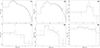 |
Fig. A.2. Spectra and best-fit models of the six X-ray AGN embedded into the MQN01 protocluster. Spectra are rebinned to ensure a minimum of 20 counts per energy bin (top panels) and 3 counts per energy bin (middle and bottom panels; see Sect. 4 for further details). |
All Tables
Conversion factors were calculated at the aimpoint and were used to convert any count rate in the energy band listed in Col. 1 to a photometric flux in the energy band listed in Col. 2.
Properties of the X-ray source candidates and the results from the best spectral-fit models.
Physical properties of the MQN01, SSA22, and Spiderweb protoclusters and their AGN populations.
Properties of the AGN host-galaxies derived from the SED-fitting analysis in Galbiati et al. (2024).
All Figures
|
Fig. 1. Chandra X-ray image in the 0.5–7.0 keV energy band, smoothed with a ∼1.5 arcsec Gaussian filter. The black squares mark the individual ObsIDs of the Chandra observations detailed in Table 1. The dashed gold lines represent concentric circles centred on the aim point in the final merged image, with radii of 6 and 12 arcminutes. Additional contours delineate the areas of multi-wavelength observations, the details of which are outlined in Sect. 3.1. |
| In the text | |
|
Fig. 2. Point source sky coverage for different Chandra observations in the soft (0.5–2.0 keV; black) and hard (2.0–7.0 keV; red) energy band. The thick solid lines mark the sky coverage of this study, while the thin solid, dotted, and dashed lines depict the sky coverage in the Chandra observations respectivley of Spiderweb (Tozzi et al. 2022), SSA22 (Lehmer et al. 2009), and Deep Field South (Rosati et al. 2002; Luo et al. 2017). |
| In the text | |
|
Fig. 3. Cumulative number of counts in the soft (left) and hard (2–10 keV; right) energy band, derived within a distance of 6 arcmin from the aim point in the Chandra data of MQN01. The red shaded area shows the uncertainties within 1σ due to photometric errors. The black line shows the number of counts predicted for the field from the AGN+Galaxy models developed in Gilli et al. (2007). |
| In the text | |
|
Fig. 4. Chandra X-ray and MUSE images of the MUSE field with symbols marking Chandra X-ray point sources and MQN01 protocluster membership candidates identified through spectroscopic and photometric methods. On the left, a 2 pixel Gaussian kernel-convolved image at the energy band of 0.5–10 keV, zoomed into the MUSE FoV (blue dashed square and blue square in Fig. 1). The red squares mark the X-ray point sources detected with S/N ≥ 3, each associated with an identity number. The blue and cyan circles show the spectroscopically confirmed MQN01 protocluster members within ±1500 km s−1 from the QSO CTS G18.01 (ID1) from MUSE (Galbiati et al. 2024) and within ±4000 km s−1 from ALMA (Pensabene et al. 2024), respectively. The green circles indicate the positions of FORS photometrically selected protocluster member candidates (Galbiati et al. 2024). The right panel shows the MUSE White Light Image of the same field with the same markers for multi-wavelength selections. |
| In the text | |
|
Fig. 5. Velocity distribution of the galaxies+AGN (white) and AGN (red) members of the MQN01 (top panel), Spiderweb (middle panel), and SSA22 (bottom panel) protoclusters, in a velocity range ±4000 km s−1 and within areas of approximately 16, 75, and 2400 cMpc2, respectively, as reported in the top left legend of each panel. |
| In the text | |
|
Fig. 6. Radial profiles, normalized to their maximum values, of the cumulative number of galaxies and AGN within a sphere of radius r < R for different protoclusters. The top, middle, and bottom panels display these profiles for galaxies (red, green, blue) and AGN (black) in MQN01, Spiderweb, and SS22, respectively. The transparent bands represent the Poissonian uncertainties in the number of objects within each sphere. The number of galaxies and AGN used to produce these curves are provided in the brackets in the legend of each panel. |
| In the text | |
|
Fig. 7. Cumulative HXLF of AGN in a volume (V16) defined to contain the bulk of the galaxy population in MQN01, with Amax ∼ 16 cMpc2 and Δvmax = ± 1000 km s−1. The red and green lines represent the HXLF estimated for the MQN01 and Spiderweb protoclusters, respectively, centred on the brightest QSOs, CTS G18.01 (ID1) and PSK1138, which are excluded from the analysis. The blue line depicts the HXLF of AGN in the SSA22 protocluster, centred at the location that maximizes the AGN overdensity within V16. The transparent bands indicate the range of values due to Poisson uncertainties. The dashed lines indicate the HXLF of AGN in the field, estimated as in Gilli et al. (2007), with the colours corresponding to the same redshifts as the solid lines for the protoclusters. |
| In the text | |
|
Fig. 8. Cumulative luminosity function of the overdensity of X-ray AGN derived as the ratio of the ϕ16 shown in Fig. 7 to the ϕ derived for the Field according to Gilli et al. (2007), normalized by the latter. The red, blue, and green curves represent the overdensities for MQN01, SSA22, and Spiderweb, respectively. |
| In the text | |
|
Fig. 9. X-ray AGN fraction versus M* threshold for different star-forming galaxy populations. The top panels display the SFR vs M* plots for galaxies in the MQN01 (red dots) and Spiderweb (green dots) regions. The Spiderweb data were obtained by Shimakawa et al. (2024) (left panel), Pérez-Martínez et al. (2023) (middle panel), and Pannella et al. (in prep.) (right panel). The shaded areas represent the Popesso et al. (2023) main sequence (MS) with a ±0.3 dex spread at redshifts z = 3.25 (red) and z = 2.16 (green). Galaxies hosting an X-ray AGN are highlighted with black-edged squares. The bottom panels show the variation of fAGN as a function of the M* threshold, as indicated by the grid of values on the x-axis. |
| In the text | |
|
Fig. 10. Probability density function (PDF) of the λsBHAR parameter for the three SMBH populations hosted in the MQN01 (red), SSA22 (blue) and Spiderweb (green) protoclusters. The solid lines represent the λsBHAR PDFs obtained using an iterative procedure that incorporates additional artificial sources, created by randomly varying LX and M* within their 1σ uncertainties. The dashed lines show the λsBHAR PDFs without applying this iterative procedure, with the number of AGN indicated in brackets in the legend. |
| In the text | |
|
Fig. 11. λsBHAR as a function of the distance from the central QSOs, CTS G18.01 in MQN01 (red) and PSK1138 in the Spiderweb (green) protocluster. The black dots mark the median values of λsBHAR for the AGN in both protoclusters across different bins of distance from the two central QSOs. The uncertainties correspond to the 16th and 84th percentile values within each radial bin. |
| In the text | |
|
Fig. A.1. Chandra X-ray images (in counts) focusing on the six X-ray sources associated with spectroscopically selected protocluster members. The images are binned in energy bands: soft (0.5-2.0 keV) in the top panels; hard (2.0-7.0 keV) in the central panels; and broad (0.5-7.0 keV) in the bottom panels. The red and orange circles denote the protocluster members identified through spectroscopic selection with MUSE and ALMA, respectively. The first column depicts the region of the three closely located X-ray detections within a FoV of 115 × 115 kpc2, while the subsequent columns present FoVs of approximately 92 × 92 kpc2, centred on the other detections. |
| In the text | |
|
Fig. A.2. Spectra and best-fit models of the six X-ray AGN embedded into the MQN01 protocluster. Spectra are rebinned to ensure a minimum of 20 counts per energy bin (top panels) and 3 counts per energy bin (middle and bottom panels; see Sect. 4 for further details). |
| In the text | |
Current usage metrics show cumulative count of Article Views (full-text article views including HTML views, PDF and ePub downloads, according to the available data) and Abstracts Views on Vision4Press platform.
Data correspond to usage on the plateform after 2015. The current usage metrics is available 48-96 hours after online publication and is updated daily on week days.
Initial download of the metrics may take a while.