| Issue |
A&A
Volume 696, April 2025
|
|
|---|---|---|
| Article Number | A234 | |
| Number of page(s) | 25 | |
| Section | Astrophysical processes | |
| DOI | https://doi.org/10.1051/0004-6361/202452040 | |
| Published online | 30 April 2025 | |
First Light And Reionisation Epoch Simulations (FLARES)
XVI. Size evolution of massive dusty galaxies at cosmic dawn from the ultraviolet to infrared
1
DTU Space, Technical University of Denmark, Elektrovej 327, DK-2800 Kongens Lyngby, Denmark
2
Birla Institute of Technology and Science, Sancoale, 403726 Goa, India
3
Cosmic Dawn Center (DAWN), Copenhagen, Denmark
4
Astronomy Centre, University of Sussex, Falmer, Brighton BN1 9QH, UK
5
Hiroshima Astrophysical Science Center, Hiroshima University, 1-3-1 Kagamiyama, Higashi-Hiroshima, Hiroshima 739-8526, Japan
6
National Astronomical Observatory of Japan, 2-21-1, Osawa, Mitaka, Tokyo, Japan
7
The Institute of Cancer Research, 123 Old Brompton Road, London SW7 3RP, UK
8
Institute of Cosmology and Gravitation, University of Portsmouth, Burnaby Road, Portsmouth PO1 3FX, UK
⋆ Corresponding author: This email address is being protected from spambots. You need JavaScript enabled to view it.
, This email address is being protected from spambots. You need JavaScript enabled to view it.
Received:
28
August
2024
Accepted:
27
February
2025
Abstract
We used the First Light And Reionisation Epoch Simulations (FLARES) suite to study the evolution of the rest-frame ultraviolet (UV) and far-infrared (FIR) sizes for a statistical sample of massive (≳109 M⊙) high-redshift galaxies (z ∈ [5, 10]). The galaxies were post-processed using the SKIRT radiative transfer code to self-consistently obtain the full spectral energy distribution (SED) and surface brightness distribution. We created mock observations of the galaxies for the Near Infrared Camera (NIRCam) to study the rest-frame UV (1500 Å) morphology. We also generated mock rest-frame FIR (50 μm) photometry and mock ALMA 158 μm (0.01′′ − 0.03′′ and ≈0.3′′ angular resolution) observations to study the dust-continuum sizes. We find the effect of dust on observed sizes is reduced with a rising wavelength from the UV to optical (∼0.6 times the UV at 0.4 μm), with no evolution in FIR sizes. Observed sizes vary within 0.4 − 1.2 times the intrinsic sizes at different signal-to-noise ratios (S/N =5 − 20) across redshifts. The effects of the point spread function (PSF) and noise makes bright structures prominent, whereas fainter regions blend with noise, leading to an underestimation (by a factor of 0.4 − 0.8) of sizes at S/N =5. At S/N =15 − 20, the underestimation reduces (factor of 0.6 − 0.9) at z = 5 − 8, but due to the PSF, at z = 9 − 10, bright cores are dominant, resulting in an overestimation (factor of 1.0–1.2) of sizes. For ALMA, low (≈0.3′′) resolution sizes are affected by noise that tends to behave as extended emission. The size evolution in UV is in overall agreement with current observational samples and other simulations. This work is one of the first to analyse the panchromatic sizes of a statistically significant sample of simulated high-redshift galaxies. These results supplement a growing body of research highlighting the importance of conducting equivalent comparisons between observed galaxies and their simulated counterparts in the early Universe.
Key words: galaxies: evolution / galaxies: high-redshift / galaxies: photometry
© The Authors 2025
 Open Access article, published by EDP Sciences, under the terms of the Creative Commons Attribution License (https://creativecommons.org/licenses/by/4.0), which permits unrestricted use, distribution, and reproduction in any medium, provided the original work is properly cited.
This article is published in open access under the Subscribe to Open model. This email address is being protected from spambots. You need JavaScript enabled to view it. to support open access publication.
1. Introduction
Galaxy sizes can provide important insights into the physical processes responsible for galaxy formation and evolution. It is one of the few parameters that can be defined independently via photometry. Sizes in various wavelength ranges across various redshifts can not only tell us about evolution of galaxy properties over time (Conselice 2014), but galaxies of various sizes and morphologies are important for constraining important relations, such the ultraviolet (UV) luminosity function (Kawamata et al. 2018), by providing a completeness measure for the data (Marshall et al. 2022). Observations have also shown that sizes of galaxies at fixed stellar mass are smaller at higher redshifts (Franx et al. 2008); hence, by studying the galaxy sizes over cosmic time, we can study galactic processes affecting the structures of galaxies and thus galaxy evolution. This evolution in galactic processes can also change the dust and gas content, ultimately affecting the observed morphology. Galaxy mergers, instabilities, gas accretion, gas transport, star formation, and feedback can all affect the sizes of galaxies (Xie et al. 2017). With new high-resolution UV and far-infrared (FIR) imaging provided by JWST and ALMA, the time is ripe for panchromatic studies of high-redshift galaxies.
At a fixed redshift the relationship between luminosity and size can be expressed as
 (1)
(1)
where R0 is a normalisation factor representing the effective radius at Lz = 3*, β1 is the slope of this relation, and Lz = 3* is the characteristic rest-frame UV luminosity for z ≃ 3 Lyman break galaxies2.
Previous studies (Shibuya et al. 2015; Holwerda et al. 2015; Grazian et al. 2012; Bouwens et al. 2022) also form the base of a growing consensus of a positive β in Eq. (1). However, the evolution of these values with redshift varies between studies. Shibuya et al. (2015) finds a constant β = 0.27 ± 0.01 and a decreasing R0 with redshift (z < 10). Holwerda et al. (2015) finds β = 0.24 ± 0.06 at z ∽ 7, which decreases to β = 0.12 ± 0.09 at z ∽ 9 − 10. Grazian et al. (2012) finds β = 0.3 − 0.5 at z ∽ 7. Huang et al. (2013) states that β = 0.22 at z = 4 and β = 0.25 at z = 5. Recent studies of Hubble Frontier Field lensed galaxies at z = 4 − 8 agrees with a positive and high β (∽0.4) value (Bouwens et al. 2022). They also show an increasing beta with increasing redshift, but the samples are limited to two bins of z = 4 and z = 6 − 8, which is insufficient to draw clear conclusions on the evolution of β.
There have also been a number of studies that have explored the size-luminosity relation and the associated physics influencing this relation at these high redshifts, using simulations of galaxy formation and evolution. Studies carried out, for example, by Liu et al. (2017) and Marshall et al. (2019), using semi-analytical models (SAMs), have reported β = 0.33 for 5 ≤ z ≤ 10 galaxies. Many hydrodynamical simulations have also explored the evolution of observed galaxy sizes at the Epoch of Reionisation (EoR, at z > 5). Marshall et al. (2022) studied the size-luminosity relations in the BLUETIDES simulation (Feng et al. 2016), which shows a decreasing positive β with increasing redshift. Using the SIMBADavé et al. (2019) simulations, Wu et al. (2020) showed a similar positive β for the FUV sizes. Roper et al. (2022) (hereafter FLARES IV) used the FLARE simulations Lovell et al. (2021), Vijayan et al. (2021) and also showed β in the range of [0.279,0.319] for redshifts 5–8 and β = 0.519 for a redshift of 9.
Galaxy size evolution as a function of redshift can be expressed as
 (2)
(2)
where R0, z = 0 is a normalisation factor corresponding to the size of a galaxy at z = 0 and m is the slope of the redshift evolution (Mo et al. 1998).
A number of studies using deep Hubble Space Telescope (HST) fields have measured the sizes of z = 6 − 12 Lyman-break galaxies (e.g. Oesch et al. 2010; Mosleh et al. 2012; Grazian et al. 2012; Ono et al. 2013; Huang et al. 2013; Holwerda et al. 2015; Kawamata et al. 2015, 2018; Shibuya et al. 2015). These observations find that high-redshift galaxies are small and bright, compared to lower-redshift galaxies, with their half-light radius (Re) in the range of 0.5 − 1 kpc at rest-frame wavelength of 1500 Å. These studies report slopes usually in the range 0.6 ≤ m ≤ 2.0 (Eq. (2)) for galaxies with LUV in the range (0.3 − 1)L .
.
The size evolution with redshift has also been studied using galaxy simulations studies. For instance, Liu et al. (2017) and Marshall et al. (2019) used SAMs and predicted m values of 1.9 − 2.2 for LUV in the range (0.3 − 1)L . These values are steeper than most observations, which is attributed to the strong supernova feedback in their model, which produces a faster evolution of average galaxy size. FLARES IV reported m values of 1.1 − 1.8 for LUV in the range (0.3 − 1)L
 . These values are consistent with observational studies mentioned above. BLUETIDES simulations Marshall et al. (2022) have shown a size evolution slope m = 0.662, which is much lower than what is seen in observations as well as other simulations. This may be the result of the simulations running only for z ≥ 7, a regime that does not have extreme growth in galaxy size.
With various studies available, there is no clear consensus on the evolution of β with redshift or m, in observational or theoretical studies. It is important to note that there are physical uncertainties in models, as in the case of the recipes for star formation and feedback used in simulations. Conroy & Gunn (2010) also discussed substantial uncertainties existing in stellar population synthesis (SPS) modelling. The choice of SPS models will affect the placement of a galaxy in the mass-luminosity-size plane. However, the relative distribution of light in the galaxy will remain the same, leading to no size variation. In addition, both observational and simulation studies use different galaxy structure definitions, as well as resolutions and observing instruments, resulting in variations among the luminosity measurements. Simulations have looked for gravity-bound particles to define a galaxy, whereas observations consider objects inside an aperture so the two datasets can differ in the structures that are identified as galaxies. Bleeding of light from nearby sources as well as background and dark sources can also play a role in the lack of agreement among such studies. Therefore, the use of similar analysis to compare models and observations becomes really important for constraining physical relations, such as the size-luminosity relation.
Size evolution analysis is hard at EoR due to galaxies being hard to detect and resolve. JWST has changed this, due to it unprecedented sensitivity in the observed near-to-mid infrared (NIR-MIR). However, in the rest-frame far-infrared (z ≥ 5), due to their lower dust content (Magnelli et al. 2020; Pozzi et al. 2021), facilities such as ALMA require significant time investment to achieve meaningful observations. Thus, there are only a handful of studies that have examined the evolution of sizes in FIR wavelengths at z ≥ 5. Using the ALMA-CRISTAL survey, Mitsuhashi et al. (2024) and Ikeda et al. (2025) evaluated the sizes of typical star-forming galaxies at redshifts of z = 4 − 6, while studying the dust-obscured star formation. They found that dust continuum sizes at 158 μm are approximately twice as extended as UV sizes. Similarly, Fudamoto et al. (2022) also found dust continuum and [C II] emission to be extended with sizes larger than FUV sizes. Pozzi et al. (2024) also found extended dust emission in FIR up to 3 kpc, with dust continuum sizes that are bigger than the UV sizes by a factor of 2. Gullberg et al. (2019) also compared K-band size with 870 μm sizes, finding 870 μm sizes being on average 2.2 times smaller than K-band sizes, albeit with majority of the sample at lower redshift (z ≲ 4). The high-redshift (z ≥ 5) ALMA studies are contrary to the findings of Popping et al. (2022) using the ILLUSTRIS-TNG 50 simulation Nelson et al. (2019), Pillepich et al. (2019) as well as FLARES IV. They credit this to clumpy gas distribution around the outskirts of galaxies or massive star-forming clumps within galaxies as major source of UV emission.
Dust in any astrophysical system will impact the radiation traveling through it by the scattering and extinction of photons and re-emitting them at longer wavelengths. This makes the observed spectra of galaxies very different from the dust-free spectra (Li 2009). The dust content in the EoR is expected to be less than in the present universe (Li et al. 2019; Vijayan et al. 2019; Magnelli et al. 2020; Pozzi et al. 2021; Yates et al. 2024). However, even small amounts of dust can lead to significant attenuation in the UV (Behrens et al. 2018; Liang et al. 2019; Ma et al. 2019). This absorbed energy is re-emitted in the IR. Thus, studying size evolution in the IR is equally important to understand the dust properties and its evolution in galaxies. The distribution and composition of dust in a galaxy can lead to variability in the amount of dust extinction, decreasing the observed luminosity for dusty regions (Witstok et al. 2023; Markov et al. 2025; Shivaei et al. 2024). Cochrane et al. (2024) used FIRE simulations to show that heavy dust obscuration in certain lines of sight (LoS) can cause galaxies being unobservable. The higher the wavelength, the lesser dust affects the radiation (Marshall et al. 2022, FLARES IV). Since size measurement is based on the observed luminosity, this decrease in luminosity caused by dust will also bring variation in the observed size-luminosity or size-redshift evolution relations. This kind of size variation between mock observations and dust-free sizes has been reported in the THESAN simulations (Shen et al. 2024), with median dust-free UV sizes being lower than dust attenuated sizes (factor of 1–0.33), with the differences increasing with stellar mass (see Fig. 16 in their paper).
Radiative transfer in astrophysical systems can be simulated to calculate the effect of dust and scattering of light away and into the LoS to get realistic emissions at different wavelengths. This work uses the SKIRT radiative transfer code (Camps & Baes 2015, 2020) to post-process a sample of galaxies in the FLARES suite of simulations (selection criteria are discussed in Sect. 2.2) and generate their spectral energy distributions (SEDs) as well as the surface brightness profile in the UV and IR. FLARES was chosen to get a statistical population of massive galaxies (≳109 M⊙) in the EoR. We then used the results of this radiation transfer simulation to explore the size-luminosity relation and size evolution of galaxies in the epoch of re-ionisation in the UV and FIR regimes. We also compared it with a similar analysis in the UV on FLARES galaxies based on a LoS method (as discussed in Vijayan et al. 2021) in FLARES IV. Such a panchromatic study of galaxy sizes is also very relevant and timely, given the wealth of multi-wavelength data expected in the next decade. This analysis will enable us to study the disparity between the intrinsic galaxy sizes and what can be observed with the best instruments available.
In Sect. 2, we detail the FLARES simulations and choices made in SKIRT, while also detailing the methodology used to make synthetic photometry and mock observations. We also discuss methods of size calculation used. Section 3 expands on the effect of noise and PSF which leads to variation in observation sizes against simulation sizes. In Sect. 4, we analyse the galaxy size evolution in UV against redshift, luminosity, and mass. We also compare the size disparity between observations and simulations in this section. Section 5 discusses the IR galaxy size evolution with respect to redshift and mass. Section 6 presents a panchromatic analysis between the UV and FIR spectrum sizes. We present our conclusions in Sect. 7. We use a Planck year 1 cosmology throughout this paper, corresponding to Ωm = 0.307, ΩΛ = 0.693, and h = 0.677.
2. Methodology
2.1. The FLARE simulations
The First Light And Reionisation Epoch Simulations (FLARES, Lovell et al. 2021; Vijayan et al. 2021) suite offers zoom-in simulations of 40 regions chosen from a 3.2 cGpc a side dark matter only box. FLARES has the same gas and dark matter mass resolution as EAGLE (mg = 1.8 × 10⁶ M⊙ and mdm = 9.7 × 10⁶ M⊙, respectively). These regions were re-simulated until z = 4.67 with full hydrodynamics using the AGNdT9 configuration of the EAGLE (Schaye et al. 2015; Crain et al. 2015) galaxy formation model (see Table 3 in Schaye et al. 2015). This configuration produces similar stellar mass functions to the reference EAGLE model. This configuration gives more energetic, less frequent AGN feedback events and it is better at reproducing the gas mass fractions of low-mass galaxy groups compared to the reference EAGLE model. The resulting properties, such as the UV luminosity function, have been shown to converge to observational constraints in Lovell et al. (2021) and Vijayan et al. (2021).
The regions were selected at z = 4.7, with a radius of 14 cMpc/h, spanning a wide range of overdensities, from δ = −0.479 to 0.970 (see Table A1 in Lovell et al. 2021). The regions are deliberately selected to contain a large number of extreme overdense regions (16) to obtain a large sample of massive galaxies. Two regions each were also selected at each overdensity, multiples of the standard deviation (n × σ) derived by fitting a Gaussian function to the log(1 + δ) distribution, with n = [4, 3, 2, 1, 0.5, 0, −0.5, −1, −2, −3]. Additionally, two mean density regions were chosen, to increase the sampled volume of these common regions, along with the two most underdense regions (δ ≈ −0.45) to cover the whole dynamic range. These total up to 40 regions. The simulations were run with a heavily modified version of PGADGET-3 an N-Body Tree-PM smoothed particle hydrodynamics (SPH) code (same as EAGLE, last described in Springel et al. 2005).
The FLARES regions are predominantly biased towards extreme over-density regions within the dark matter simulation box. This choice provides FLARES with a statistically significant sample of massive galaxies in the early Universe, which are expected to be biased towards such regions (see Chiang et al. 2013; Lovell et al. 2018). To remove the bias towards overdense regions and to ensure a representative sample, a weighting scheme (described in Sect. 2.4 in Lovell et al. 2021) is used when calculating mean-median statistics.
2.2. Galaxy selection
A friends-of-friends algorithm (FoF, Davis et al. 1985) was used to find bound groups in the simulations. Amongst these bound groups, galaxies in FLARES were identified with the SUBFIND algorithm (Springel et al. 2001; Dolag et al. 2009). This algorithm finds saddle points in the density field of a FoF halo to identify self-bound substructures. The most bound particle of these structures is denoted as the centre of our galaxies. The stellar mass of a galaxy in the simulation is defined based on the star particles present within a 30 physical kpc (pkpc) radius around this centre. The same selection criteria as in Vijayan et al. (2022) (hereafter FLARES III) was used to generate our dataset. We only included galaxies with ≥1000 star particles to ensure our sample is well resolved. This is done so that the galaxies are well defined physically and also have enough data for a subsequent Monte Carlo radiative transfer. This selection criteria leave us with galaxies of a stellar mass of M⋆ > 109.12 M⊙ and UV luminosity of LUV,1500 Å > 1026.9 erg/s/Hz. We refer to Table 1 for the details of the mass bin distribution.
Distribution of galaxies across different redshifts and mass bins.
2.3. SKIRT modelling
In this work, we used the SKIRT (Camps & Baes 2015, 2020) radiative transfer code to construct rest-frame UV and far-infrared images of the FLARES galaxies. Overall, SKIRT is set up to simulate each galaxy in our selection. The set-up is the same as described in FLARES III, with a brief description provided here. The SEDs of young stellar populations (age ≤10 Myr) are modelled using the MAPPINGS III (see Groves et al. 2008, for more details) template. These were produced using the MAPPINGS III photo-ionisation modelling code, to model the nebular emission from young stars. The model assumes the STARBURST99 SPS code Leitherer et al. (1999) for the stellar tracks and a Kroupa IMF Kroupa (2002). The older populations (age > 10 Myr) are modelled using the BPASS (see Stanway & Eldridge 2018, for more details) SPS code, assuming the Chabrier IMF. We assumed a Weingartner & Draine (2001) SMC type dust mixture to simulate dust emission and attenuation effects, with the effect of self-absorption by dust taken into account. We took into account the heating of dust by CMB, because at these redshifts (z = 5 − 10), the CMB temperatures can be comparable to dust temperatures, affecting the observed luminosities. Furthermore, as all these radiative transfer results are estimated by SKIRT using Monte Carlo Method, a higher number of simulated photons would lead to a more accurate result; hence, we used 106 photon packets per radiation field wavelength grid (Appendix A in FLARES III shows that increasing the photon count has negligible effect on radiative transfer results with obtained SEDs by using 106 and 107 photon packets per wavelength grid converging). Other factors such as the distribution of sources, dust and gas, and the dust mass fraction were defined for each galaxy based on the FLARES star and gas particle data, similarly to the approach to FLARES III.
The observational instruments in SKIRT are set up at a distance of 1 Mpc from the galaxy and have a field of view (FoV) of 60 × 60 pkpc2. This whole field of view is captured in a 400 × 400 pixel frame (this corresponds to a per pixel resolution of 0.023″, 0.026″, 0.028″, 0.030″, 0.033″, and 0.035″ for redshifts 5 through 10, respectively)3. The plane on which these galaxies are observed is the same and, hence, the orientation of the galaxies in FLARES automatically leads to different viewing angles. It is only at the highest redshifts (z ≥ 9) – corresponding to the most massive galaxies (M⋆ ≥ 1010 M⊙), where there is a dearth in the number of galaxies sampled in FLARES (see Table 1) related to a high disc galaxy fraction (see Ferreira et al. 2023) – that we would see an increased effect with respect to the viewing angle (face-on or edge-on)4. Based on these parameters, we obtained a per-pixel SED for the UV and the IR spectrum, as well as the SED for the range [0.08,1500] μm for the whole FoV. The images are centred on each galaxy’s centre of potential as calculated by SUBFIND.
2.4. Comparison with the LoS method of previous studies
In this work, we have employed SKIRT to produce synthetic images, however, in most previous works on FLARES, we have adopted a simpler approach to produce synthetic observations, including spectra and imaging. The LoS method (as discussed in Vijayan et al. 2021) estimates the effect of dust attenuation by calculating the intervening column density of dust. This can then be converted to an optical depth measure by assuming a dust extinction curve. Anisotropic scattering by the dust couples all lines of sight and dust absorption and/or emission couple all wavelengths, making the radiative transfer equation highly non-local and non-linear (Steinacker et al. 2013); however, this is not taken into account in the LoS method because of its complexity. However, the star-dust geometry is preserved. Radiative transfer using a Monte Carlo simulation to estimate these effects in both absorption and scattering by dust grains. Thus, this approach can self-consistently generate the dust emission in the IR, which is the major motivation for using SKIRT outputs in this study. Figure 1 shows the radiative transfer luminosities, which are ≈0.2 − 0.3 dex lower than the LoS luminosities. It also illustrates the additional effects that are not accounted for in the LoS method but contribute to the observed variation in luminosities between the two approaches. Also, in previous studies, in the LoS method, the free parameters that are used to calculate the dust attenuation were chosen to match the UV luminosity function at z = 5 (see Sect. 2.4 in Vijayan et al. 2021). This difference in method of calculating the dust attenuated luminosity will cause the intercept and slopes of the size-luminosity relation to differ in the two methods. Section 4.2 shows this difference aptly when compared with slopes and intercepts found in the Appendix B of FLARES IV. Appendix E in Vijayan et al. (2022) also compares the UV luminosity function obtained by using the LoS method and radiative transfer for the same sample of galaxies as this study. Vijayan et al. (2022) also found the normalisation of radiative transfer results to be 0.4 dex lower than LoS model, attributing it mainly to the lower dust optical depth along the LoS adopted in LoS studies of FLARES galaxies compared to the radiative transfer method.
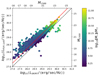 |
Fig. 1. Luminosity from SKIRT radiative transfer (estimated at 1500 Å) on x axis is compared with LoS luminosities (as discussed in Vijayan et al. 2021) on y axis. Luminosity from the LoS method is roughly 0.25–0.3 dex higher than luminosities produced by radiative transfer. The red line is the best fit offset between the two luminosities. The colours corresponding to the colourbar shows the average stellar mass in each hexbin. |
2.5. Size calculation
To measure sizes, observational studies generally use either Sérsic profile fitting (Sérsic 1963) or a curve of growth method (Stetson 1990; Ferguson et al. 2004; Bouwens et al. 2004; Oesch et al. 2010) based on circular or elliptical apertures. Sérsic profile fitting causes variation in sizes compared to the curves of growth sizes in case of a clumpy nature of high-redshift galaxies (Jiang et al. 2013; Bowler et al. 2022). Clumpy galaxies are elongated in nature with multiple separated bright parts, amongst which centre selection plays an important role in half-light radius calculation and affects the size calculated. In simulations, particle distributions can also be used to find the radius enclosing half of the light or mass to determine sizes. Since our aim is to simulate observations and calculate their disparity with observed sizes, we used the commonly used circular apertures (Bouwens et al. 2004; Oesch et al. 2010) as well as curves of growth (luminosity contained inside a radius) to define our half-light radius. We used two different methods to do so, as described below. Previous FLARES works (FLARES IV) have also used a non-parametric pixel based method (e.g. Bowler et al. 2017) to calculate sizes. A comparison of the two methods is also presented below.
Iterative aperture method
We calculated the total luminosity in the galaxy image by summing all pixels within the FoV. For calculating sizes (half-light radius) using the iterative aperture method, we started with the centre of potential of the galaxy. We calculated total luminosities in circular apertures of given radius R (starting with R = 0) from the potential centre in increments of 1 pixel until the flux inside the aperture exceeds three-quarters of the total luminosity of the FoV. Then, using the radii and their corresponding luminosity we interpolate the half-light radius (radius with half the total luminosity of the image) converted to pkpc.
statmorph
statmorph5 (Rodriguez-Gomez et al. 2019) is an open source python package that segments an image to look for objects and calculates their morphological properties. It provides the centre of the object, its radius at various light fractions, concentration, asymmetry, clumpiness and Gini-M20 statistics. In this study, we used statmorph on our mock images to get morphological properties for the galaxies if they were observed at different signal-to-noise ratios (S/Ns), as discussed in Sect. 2.6.1.
We used the iterative aperture method to calculate sizes for high resolution, noise, and PSF free SKIRT outputs. These sizes are denoted as ‘intrinsic sizes’ or ‘Re, intrinsic’ throughout the following paper, as these denote the size of galaxies with no observational effects at play. The iterative aperture method was used for these outputs as clumpy or dispersed galaxies with few connecting pixels are segmented as separate objects while using statmorph. Overall, statmorph is used to calculate sizes for all simulated imaging that contains observational effects. These sizes are denoted as ‘observed sizes’ or ‘Re, obs’ throughout the paper. Appendix A shows that for noise and PSF free SKIRT output that can be segmented properly, with the sizes calculated by both these methods converging to a 1:1 relation.
Comparison with non-parametric pixel method
FLARES IV used a non-parametric pixel approach to calculate the half-light radius (denoted by Re, non − parametric). In this method, the pixels of the image are ordered from most luminous to least luminous, and then the pixel area containing half the total luminosity is taken into account to calculate the half-light radius assuming a circular aperture. This method is used to account for the clumpy nature of galaxies at high redshift. As this method gives the radius assuming the most compact morphology possible, the sizes calculated by our curves of growth method using circular aperture are higher as they are dependent on structure. This is clearly seen in Fig. 2, where we plot the sizes from pixel method against the sizes from curves of growth method for 1500 Å.
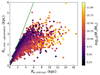 |
Fig. 2. Comparison of the half-light radii at 1500 Å using the method from FLARES IV and this studies’ circular aperture method is shown above. The calculated HLR from a non-parametric pixel-based method is plotted on the y-axis with the intrinsic sizes plotted on the x-axis. Sizes from non-parametric pixel method are lower than intrinsic sizes used in this study due to non-parametric pixel method accounting for the most compact configuration of the galaxy. The green line shows the 1:1 relation. |
It is important to note that for a direct comparison between FLARES IV, resolution also plays a role. In contrast to using the softening length (s = 2.66/(1 + z) pkpc) resolution, this study uses a fixed 400 × 400 pixel resolution for intrinsic sizes irrespective of redshift. All UV observational analysis in the study uses JWST resolutions as described in Sect. 2.6.1.
2.6. Photometry/image creation
2.6.1. NIRCam
For generating our mock observations, we used a rest-frame wavelength of 1500 Å, corresponding to the far-UV. We made mock observations for JWST NIRCam’s filters: F090W, F115W, F140M, F150W, and F162M, depending on the redshift. In the wavelength range of 0.6–2.3 μm observations, the NIRCam resolution is 0.031″/pixel. Using the field of view from SKIRT and distance (i.e. redshift), we regridded the images produced from SKIRT to the NIRCam resolution (see Table B.1).
To mock the observational effects of NIRCam observations, the images were convolved with a point spread function (PSF) for different filters, corresponding to the observed (redshifted) wavelength. We used the PSFs from JWST PSF simulation library, simulated by WebbPSF (Perrin et al. 2012, 2014), provided by STScI. To the convolved images we added shot and Poisson noise. To account for the sky background noise, the images were also further modified with Gaussian noise after PSF convolution. To analyse the effect of noise mathematically, noisy mock image was generated uniquely for each source at different S/Ns (5–20). Figure 3 shows the evolution of image through various stages described above and Fig. 4 shows a sample of NIRCam RGB false colour images (F200W, F150W, F115W) for galaxies in different mass bins. We then evaluated results at a S/N of 5, 10, 15, and 20 (corresponding to exposure times of approximately 5, 14, 40, 70 minutes at z = 5 for an observations similar to CEERS (Holwerda et al. 2024) for a representative galaxy with NIRCam (F090W) flux), to see the effect of observation time on the observed sizes.
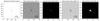 |
Fig. 3. Sample galaxy image at z = 5 at various stages of methodology, in a 60 × 60 pkpc2 field of view. First panel: Result of SKIRT radiative transfer simulation. Second and third panels: Mock observation produced after regridding to 302 × 302 pixels based on Near Infrared Camera (NIRCam) resolution at this redshift and adding the effects of Gaussian + shot noise corresponding to S/N =5 and PSF is shown in the second panel with its respective segmentation map in the third panel showing only a single detected object. Fourth and fifth panels: Simulated imaging, as described earlier, but it is shown at S/N =15 in fourth panel, with its respective segmentation map and showing three distinct objects detected in the fifth panel. |
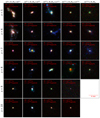 |
Fig. 4. False colour images from the previous figure, here showing sample galaxies at different redshifts and various mass bins at S/N =20. The FoV of the images is 20 pkpc and the red, green, and blue channel taken from JWST/NIRCam F200W, F150W, and F115W filter data, respectively. |
We used detect_sources from the photutils (Bradley et al. 2023) library to create a segmentation map (sources are defined with 1.5σ detection and a criterion of 5 minimum connected pixels). Depending on the background S/N added to the image, our segmentation maps can differ. This can be seen in Fig. 3, which shows three separate objects detected at S/N =15, whereas at S/N =5, two of these objects blend with noise and are not segmented. The segmentation algorithm which takes into account the minimum number of connected pixels for an object; hence, it can identify two or more objects from a single galaxy image. In these cases, we considered the brightest source as our galaxy. This also resolves cases of mergers with the two distinct cores being segmented as separate objects and only one of them being selected for size analysis. We also evaluated our galaxies by simulating observations for being a part of a large survey with each galaxy embedded in a Gaussian noise field with a fixed standard deviation for all the sources. The effect of such an analysis is present in Appendix E. For all subsequent analyses, the results of the S/N =5 imaging have been used, unless explicitly stated otherwise.
2.6.2. IR imaging
We created imaging for at high-resolution IR for a FIR hypothetical instrument similar to NIRCam. To also compare to current observational studies, we also simulate mock ALMA imaging of the FIR dust-continuum at rest frame 158 μm. We used simobserve task in CASA (CASA Team 2022) to create the measurement set. We simulated the ALMA observations with two different resolutions. All three of these IR imaging techniques are described below:
-
High Resolution NIRCAM like imaging: We used the per pixel SED data for the far-infrared from our radiative transfer simulations. At these high redshifts, there are no similar observatories (without unrealistic observational time required) with as high a resolution as JWST in the rest-frame IR (the highest resolution channel on the Herschel Space Observatory was 5 arcsec). Thus, we created an arbitrary PSF from a 2D Gaussian kernel with a standard deviation of 2 pixels (0.052″ at z = 5) for adding observational effects to our images. Gaussian and shot noise were also added. We simulated the noise for S/N =5, 10, 15 and 20, but stuck to using S/N =5 for all subsequent analyses. We carried out this process for 50 μm and 250 μm wavelengths. There is no significant sizes evolution with wavelength for our sample, as shown in Sect. 5.3; hence, we used the 50 μm mock photometry for all further analysis. This being a simulated photometric imaging, the sizes for these images will be denoted by Re, obs, IR, phot.
-
ALMA Low angular resolution: We also simulated observations with similar parameters as presented in the CRISTAL survey (Mitsuhashi et al. 2024). We used the C3 configuration for ALMA, which leads to a resolution of ≈0.3′′. The resulting images (for the same sample of galaxies as in Fig. 4) are shown in Fig. 5. The sizes for these images will be denoted by Re, obs, IR, alma − lr.
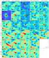
Fig. 5. Sample of galaxies (same galaxies as in Fig. 4) as observed by ALMA at 158 μm at an aperture of 30 pkpc. Low angular resolution (≈0.1′′) (similar to CRISTAL program) is used. The beam size is shown by the circle at bottom left corner. The black contours show four linearly spaced contours between brightest pixel to 1/4th of brightest pixel for 1500 Å.
-
ALMA High angular resolution: We simulated observations with ≈0.01 − 0.02′′ angular resolution, thus requiring the extended C-8 configuration. The resultant images produced are shown in Fig. H.1. The sizes for these images will be denoted in further studies by Re, obs, IR, alma − hr.
For both ALMA categories, observations were done with a bandwidth of 7.5 GHz around the redshifted frequency (rest-frame 158 μm) for our observations, with a S/N =10 level of Gaussian noise induced before ALMA simulation. ALMA beam effect is simulated on this preinduced noisy image. Due to adopting a fixed sky temperatures and zenith opacity, we observed with the ALMA S/N in the range of [3,15]. For our sample an integration time of approximately 2 hours and 40 hours per object would be required to achieve S/Ns of 3 and 15, respectively, for the ALMA low-resolution imaging. The S/Ns of most of the sample at z = 5 and 6 give a good match to the observed S/N in CRISTAL survey (Mitsuhashi et al. 2024). We set a sky temperature of 260 K for the simulation with the zenith opacity being 0.1 at the observing frequency. To analyse the simulated observations, we cleaned the obtained output by running Tclean, the inherent cleaning algorithm in CASA, for 10 000 iterations, deconvoluting the data using Hogbom CLEAN algorithm (Högbom 1974). The maximum and minimum depth of cleaning were 0.05 and 0.8 times the PSF fraction, respectively.
3. Effect of noise and PSF
The PSF describes the spread of the flux over a range of pixels for a point source due to the diffraction of light entering the optics of an observatory. The optics spreads the sources in a pattern around its surroundings, making the surrounding regions of bright sources even brighter. Along with this, Gaussian noise will increase or decrease the brightness of a pixel due to randomness of noise assignment. The relative brightness of very faint/median pixels can change significantly compared to the brightest pixel due to the addition of noise. Since we calculate the half-light radius by measuring the total luminosity inside a certain aperture and compare it with the total luminosity (i.e. we are dealing with relative brightness), this jumping of pixels to different brightness bins affects the measured sizes.
We took a sample of images from different redshifts and normalised them and then calculated average brightness of a pixel at different radii (radii are calculated from the centre of potential defined in the simulations to perform consistent analysis across all galaxies). Figure 6 compares the original radiative transfer output to the noisy image. We measure and compare the shift in luminosity profiles of the intrinsic and observed images to see the effect of noise with increasing redshift. The higher the redshift, the more the median brightness pixels are closer in magnitude to the maximum brightest pixels. It is also apparent that some luminosity of a galaxy will be lost due to noise reduction while applying a minimum threshold pixel value, also discussed in Varadaraj et al. (2024). This leads to fewer pixels being evaluated for size calculation. We show the mean percentage of pixels for galaxies in each redshift from our sample in bins of relative brightness for intrinsic and observed images in Tables 2 and 3, respectively. This impact of noise is dependent on observational parameters and filters used, affecting the depth of observations. Varadaraj et al. (2024) finds that low wavelengths filters (F115W) find a larger impact of noise on sizes than higher wavelength filters (F444W). Noise washes out faint sources effectively at low depth leading to higher offset between intrinsic sizes and the observed sizes at higher depths. We see a similar effect of noise which causes the underestimation of observed sizes. On the other hand, the PSF boosts the size of bright parts of the galaxy. This can be seen in Fig. J.1, where at S/N =15, the sizes of mock images simulated without effect of PSF added on, all observed sizes were underestimated compared to intrinsic sizes with a factor of 0.48–0.53 times. It can be seen later in Sect. 4.1 that at the same S/N, observed images show overestimation in sizes for higher redshift. This comparison also shows that the underestimation of sizes due to noise is consistent with increasing redshift, as noise primarily washes out only the faint regions of the galaxy. The effect of PSF is more significant for more compact galaxies, as bright sources when spread by the PSF, become closer (see Fig. J.2).
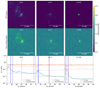 |
Fig. 6. Brightness comparison between original and noisy image is shown for a sample redshift 5, 7 & 10 galaxies with size offset at S/N =5. The bottom row shows the mean luminosity of pixels at each radius (y-axis) calculated by finding pixel luminosities at the edge of the aperture and dividing it by circumference) plotted against the radius (x-axis) for the normalised images. The centre for these luminosities is assumed as the centre of potential as defined in the simulations. The red lines indicate the maximum brightness and the green line shows the median brightness. The blue solid and dashed lines show the r20 of original and noisy image respectively. The purple solid and dashed lines show the r80 of original and noisy images respectively. Panel for z = 5 shows the case of underestimation, z = 7 of near parity and z = 10 shows an overestimation. |
Mean percentage of pixels is shown in each relative brightness bins after normalising the intrinsic images in a square aperture of width equal to 4Re (Re is intrinsic RT size).
Mean percentage of pixels is shown in each relative brightness bins after normalising the observed (S/N =5) images in a square aperture of width equal to 4Re (Re is intrinsic RT size).
Combining the observational effects of noise, pixel scale and PSF, our study shows that at lower redshifts (z = 5 − 8) galaxy centres are not extremely bright relative to the median luminosity regions, and hence Gaussian noise and PSF are able to move many pixels to a higher luminosity. Due to the effect of PSF, observed images have bright centres that are spread out, while the low luminous parts of a galaxy blend with noise. The loss of luminosity to noise triumphs the effect of PSF at lower S/N resulting in a increment of the r20 (radius at which 20 per cent of the light is present) and a reduction of r80 (radius at which 80 per cent of the light is present). This leads to underestimation (0.4–0.6 times) of the galaxy sizes at lower redshifts. With increasing redshift, the galaxy centres are comparatively brighter and compact which is further strengthened by the PSF. This leads to underestimation of sizes with higher factors (0.7–0.9 times), as compared to lower redshifts. With increasing S/N and redshift, a lower number of less luminous parts of the galaxy blend into the noise. As the FLARES galaxies are more compact at higher redshift, the loss of low luminous regions is compensated by the PSF in bright centres, leading to similar r20. The luminosity shift to the centre remains larger than the luminosity lost due to noise; hence, r80 and r50 increase. Thus, the sizes of galaxies are being overestimated at high redshift and high S/N. This change of r20 and r80 can be seen in Fig. 6 for individual samples at z = 5, 7, and 10 for which the sizes are: underestimated, nearly the same, and overestimated, respectively. Figure E.1 also shows the change in r20 and r80 described above, averaged over the whole sample for galaxies with underestimated and overestimated sizes.
4. UV size analysis
In this section, we analyse how the UV sizes evolve with cosmic time, luminosity, mass and also wavelength. We compare sizes in our study with prominent observational and simulation studies. We also analyse the variation of galaxy sizes at 1500 Å between simulations and mock observations.
4.1. Intrinsic vs. observed sizes
Mock observations using simulations have shown stark difference between observed and intrinsic size evolution relations. Galaxies in the BLUETIDES simulation (Marshall et al. 2022) show a negative dust-free size luminosity relation at z = 7, which when evaluated for dust attenuation results in a positive relation. Similarly in FLARES (FLARES IV) negative dust-free size stellar mass and dust-free size luminosity relations also show a positive correlation for dust attenuated sizes. Although the SIMBA simulations Davé et al. (2019), uniquely shows positive correlation for dust-free and observed size with mass (Wu et al. 2020). Costantin et al. (2023) also found simulated observed sizes for massive galaxies at 2 μm and 3.6 μm to be larger than dust-free stellar mass sizes at lower redshift (z = 3, 4), attributing it to mass being more compact than observable stellar light, predicting heavy dust obscuration.
Similarly to the above studies, we compared the variations between mock observational sizes and our intrinsic sizes to analyse the observational effects causing the variation in size evolution relations. Figure 7 compares the sizes from mock observations and intrinsic sizes for each of the redshift (0.40–1.16 times) at S/N =5. The best fit size relation at other S/N =10, 15 and 20 is also presented in Table 4. The figure shows a significant variation in observations and simulation sizes. From Table 4 it can be clearly seen that observational sizes will be underestimated (0.40–0.94 times) for all redshifts for S/N < = 10. For higher S/Ns for lower redshift (z ∈ [5, 6, 7, 8]) sizes will be underestimated (0.64–0.83 times) while the sizes for higher redshift (z ∈ [9, 10]) will be slightly overestimated (1.04–1.16 times) compared to intrinsic sizes. THESAN simulations (Shen et al. 2024) also shows a similar variation in size with galaxies with 107 > M∗/M⊙ > 109 having median simulation size being greater than up to three times the observed sizes with increasing stellar mass. This variation in sizes is primarily due to observational effects (PSF and noise) as the offset is independent of galaxy properties like stellar mass and FUV luminosity (see Fig. D.1). A further explanation of observational effects is given in Sect. 3.
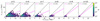 |
Fig. 7. Observed UV sizes from mock images (y-axis) are plotted as a function of intrinsic sizes (x-axis) at S/N =5. The black dashed line is a 1:1 relation whereas the magenta line is the best fit y = mx relation where y is observed size and x is intrinsic size. |
Slopes of the best-fit lines (y = mx, no intercept), where y is the mock image’s effective radius and x is the simulation’s effective radius at different S/Ns.
The sizes from mock images are calculated by statmorph, while as centre of potential is known to us from simulation, we calculate the intrinsic sizes using the iterative aperture method (as discussed in Sect. 2.5). With the effect of noise decreasing with increasing S/N at high redshift, we see that most sizes are overestimated. With the noise being primarily responsible for washing away fainter parts of the galaxy, along with the PSF intensifying the bright parts of the galaxy, this effect (with increasing S/N) shows the difficulty accounting for the complex PSF which causes the overestimated sizes (see Sect. 3).
4.2. UV size-luminosity relation
We binned our data in luminosity bins of 0.3 dex and calculated the median luminosity and median sizes in these bins. We fit Eq. (1) to these medians. Figure 8 shows a luminosity-size fit for our sample across different redshifts compared to observational and simulated data.
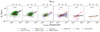 |
Fig. 8. UV luminosity size relation at different redshifts is shown. The y-axis shows the UV 1500 Å sizes in kpc and the x-axis shows luminosity at the same wavelength. The green scatter shows our sample of galaxies analysed with radiative transfer and then simulated observations for NIRCAM. The red plots show the median luminosity and sizes in bins of 0.3 dex in luminosity with 16th and 84th percentile error bars. The black line is an linear fit to the median luminosity and sizes fit to the power law. We also compare our sample with observational studies (Holwerda et al. 2015; Bouwens et al. 2022) and simulations (Marshall et al. 2022, FLARES IV). JWST data have been taken from Morishita et al. (2024) and Ormerod et al. (2024) for the sample with M∗/M⊙ ≥ 109 from the JADES (Eisenstein et al. 2023), CEERS (Holwerda et al. 2024), and PRIMER survey. |
We see a positive β in agreement with major observational studies (Holwerda et al. 2015; Grazian et al. 2012; Bouwens et al. 2022), with our observed size slopes matching these studies well at z = 5, 6 and 7 but the slopes at z > 7 are shallower with high-error margin. Our intrinsic slopes are significantly higher (> × 2) than our observed slopes. Observations compared to simulations lack very dispersed galaxies in their sample. For our dispersed galaxies at lower S/N (< 10), with low surface brightness, majority of the galaxy, blends with noise, leading to very compact observed sizes. These dispersed galaxies also flatten the size luminosity fit, leading to lower observed slope values than our intrinsic slopes. Also in contrast to other studies we see a non-evolving β (see Table 5, similar to Shibuya et al. 2015) for z = 5, 6 and 7. In Fig. 9 we compare our β slopes for both intrinsic and observed sizes with other simulations and observations at z = 7, a common redshift that is used in comparisons across simulations and observations at high redshift. When compared with observations (Holwerda et al. 2015; Huang et al. 2013; Bouwens et al. 2022), our simulated observed slope at S/N =5 is in agreement with all the studies. Our observed slopes are a bit shallower than early JWST studies like (Yang et al. 2022) but compared to recent observations (CEERS, PRIMER & JADES data taken from Morishita et al. 2024; Ormerod et al. 2024) we match the scatter at z ≥ 6 well. Although we do find a lack of ultra compact, low luminosity sample in our dataset at z = 5, 6.
β at different redshifts for radiative transfer output and the mock images (S/N =15) created.
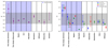 |
Fig. 9. Left: Comparison of the size-luminosity slopes (β) in relation with other studies (Roper et al. 2022; Liu et al. 2017; Marshall et al. 2022; Bouwens et al. 2022; Shibuya et al. 2015; Holwerda et al. 2015; Grazian et al. 2012) at z = 7 (blue shaded region are simulation studies) is shown. Right: Comparison of the UV size evolution slopes (m) in relation with other studies (Roper et al. 2022; Marshall et al. 2022; Oesch et al. 2010; Holwerda et al. 2015; Kawamata et al. 2018; Ono et al. 2013; Shibuya et al. 2015) is shown. |
We also plotted the size-luminosity relations at different wavelengths to see how the effect of dust evolves as a function of wavelength (see Fig. C.1). When the effect of dust is evaluated at a fixed redshift, dust causes the total luminosity to decrease and as a result size increases due to dust obscuring the bright centres of the galaxies. With increasing wavelength, the decrease in luminosity is lesser, while the sizes decrease. This makes the best size-luminosity fit decrease with increasing wavelength in the figure. This follows well with the work in Marshall et al. (2022) and FLARES IV. A comparative luminosity-size relation with non-parametric size calculation is present in Fig. I.1
4.3. UV size evolution with redshift
We also explore the evolution of sizes with redshift. Since intrinsic luminosity is related to stellar mass, we bin the data in mass bins of 0.5 dex. Higher mass galaxies tend to have a higher luminosity. We then choose the mass bin of 9.5 < M∗/M⊙ < 10 which is commonly used in literature (Shibuya et al. 2015; Mosleh et al. 2012). This bin is also sufficiently populated in all redshifts with a good spread of luminosities. As the sizes vary with luminosities as shown previously, we fit Eq. (2), for our sizes, for this mass bin as three different luminosity samples:
-
1.
 ,
, -
2.
 ,
, -
3.
 .
.
For the UV luminosity bins, the observed size slopes are m = 1.71 ± 0.25, 1.14 ± 0.31, 1.22 ± 0.40 and R0 = 30.10 ± 14.67, 13.12 ± 10.30 and 11.61 ± 6.96 respectively6. Figure 9 compares our slopes with other previous FLARES work and simulation studies and shows higher slopes for intrinsic sizes, with m = 2.23 ± 0.47, 2.46 ± 0.25, 2.45 ± 0.13 and R0 = 112.73 ± 101.59, 205.68 ± 99.40 and 197.23 ± 48.73. This difference in slope evolution is largely due to the observational effects described in Sects. 3 and 4.1, with the underestimation of observed sizes decreasing with increasing redshift, the size evolution curve becomes flat with high intercept (R0) factors. Intrinsic sizes for all three luminosity bins have similar median sizes at z = 5 but with increasing redshift lower luminosity sample tends to be more compact than higher luminosity sample. This results in low luminosity bins having lower intercepts and slopes, which also follows well with previous FLARES work (Roper et al. 2022). For observational sizes these lower luminosity sample being more compact leads to a stronger effect of PSF flattening the evolution curve, which leads to higher slopes and intercepts with m = 1.71 for the lower luminosity bin and m = 1.14 and 1.22 for higher luminosity bins, due to the fit being flattened. Figure 9 also compares our intrinsic and observed size fits to other studies. For observed sizes, the slopes of all our luminosity bins fall within the range of m = 1.0 − 2.0, similar to Ma et al. (2018) and also near the viral radius size-evolution slope m = 1.0 and m = 1.5 of dark matter halos (Mo et al. 1998; Mo & White 2002; Ferguson et al. 2004). We are also in agreement with Oesch et al. (2010) for 0.3Lz = 3* > LUV and Lz = 3* > LUV > 0.3Lz = 3* bins, while also matching Shibuya et al. (2015), Ono et al. (2013) and Kawamata et al. (2018) for the later. Holwerda et al. (2015) is one of the very few studies for very bright galaxies at high redshift reporting a m = 1.32 ± 0.43; we note that our brightest luminosity bin matches within the error margin of that study.
4.4. UV size evolution with stellar mass
UV size evolution against stellar mass has been analysed in simulations using THESAN (Shen et al. 2024). The dust-free sizes of galaxies show a negative correlation with increasing stellar mass (M∗/M⊙ ≥ 108.0) with the dust-attenuated sizes showing a positive correlation with increasing stellar mass. Our intrinsic sizes (noise and PSF free) with FLARES also shows a positive correlation with stellar mass as our sizes also account for radiative transfer effects of dust attenuation and extinction. FLARES IV has also shown that dust attenuated sizes can be nearly 50 times the simulation sizes.
Figure 10 shows median galaxy stellar masses (bins of 100.5 M⊙) plotted against the intrinsic and observed UV sizes. The intrinsic UV sizes of galaxies show an increasing slope with increasing stellar mass. For galaxies with the same stellar mass, those at lower redshift will be larger in size. Adding observational effects, we find a near flat evolution at all redshifts for observed sizes which turns negative at higher stellar mass (M∗/M⊙ ≥ 1010.5). The effect of noise in observations eats away at the faint galaxy regions outside bright cores reducing the size for galaxies with non-compact complex morphologies. This effect gains significance the more massive a galaxy is, flattening the observed evolution curve compared to the intrinsic one. This is further supported by the fact that the evolutionary trends of intrinsic size are successfully recovered for mock observations with minimal noise (S/N =50 and S/N =100 size-mass relations are shown in Fig. K.2). Similar to our study Costantin et al. (2023), using TNG50, simulated NIRCam observations using radiative transfer. They also predict near flat observed size-stellar mass relation at z = 5 which turns negative at z = 6. LaChance et al. (2024) using ASTRID simulations, found flat slopes for simulated NIRCam F444W observations at z = 5, 6 while also finding the correlation between mass and size decreasing with increasing redshift (from z = 3 to z = 6). As seen in Fig. 10 our observed sizes match the observational scatter of CEERS z = 5 − 8 galaxies from Ormerod et al. (2024). Observations compared to simulations, particularly FLARES, lack statistically significant number of galaxies at higher mass end (M∗/M⊙ ≥ 1010.5), making the high-redshift size-mass relation difficult to constraint. Although in recent CEERS survey, Ward et al. (2024) has shown a positive correlation between stellar mass and sizes (at 5000 Å). Compared to Ward et al. (2024), Costantin et al. (2023) and LaChance et al. (2024) we have higher intercepts due to probing observed sizes at a shorter wavelength.
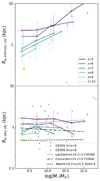 |
Fig. 10. Upper panel: Evolution of the UV simulation sizes (y-axis, in kpc) as function of stellar mass (x-axis) for z ∈ [5, 10]. Lower panel: Evolution of sizes from mock observations as function of stellar mass. Size mass relation for simulated observations from Costantin et al. (2023) and LaChance et al. (2024) and NIRCAM observations from Ward et al. (2024). CEERS data has been taken from Morishita et al. (2024) and Ormerod et al. (2024). |
5. IR size analysis
We compared the sizes in the FIR regime using various methods to study the spectrum. We also discuss the size evolution against cosmic time and stellar mass while also drawing comparisons to observational studies below.
5.1. Comparison of IR sizes by various methods
We used the IR photometric images and ALMA images (produced as described in Sect. 2.6.2) and calculated the sizes using using statmorph, as discussed earlier. Intrinsic sizes are bigger than both high-resolution ALMA and photometric sizes. Figure 11 compares the intrinsic sizes measured using the high-resolution observation methods, 50 μm photometry and ALMA mock imaging (≈0.01 − 0.02′′ angular resolution). It shows that interferometric ALMA sizes at high resolution will be able to measure sizes with a higher accuracy than NIRCam like photometry in IR when evaluated for S/N ≈ 5. This is due low-luminosity emissions blending with noise in photometry. For ALMA at this high resolution, the low-surface brightness extended emissions of a galaxy will be lost. The effect of noise and PSF (similarly to the UV case) are present in photometric imaging. This can be seen when comparing Figs. H.1 and H.2 at z = 6 sample’s lowest mass bin.
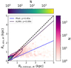 |
Fig. 11. Comparison of sizes between various IR observation methods is shown above. The plot compares IR sizes (y-axis) from mock photometry (50 μm) and ALMA simulations (high-resolution, ≈0.01 − 0.02′′ at 156 μm) with intrinsic sizes (50 μm) (x-axis). The hex-bin plot shows the log mapped distribution of photometric sizes whereas the contours show the log mapped distribution of mock ALMA sizes. The black line shows the 1:1 relation with the yellow line showing the best-fit y = mx relation. All ALMA sizes in this plot of high angular resolution (≈0.01′′ angular resolution). |
For ALMA observations at lower resolutions than this (≈0.3′′ angular resolution), small scale structures in the galaxy can be resolved to a certain extent. We compared our ≈0.3′′ lower angular resolution ALMA sizes to the high angular resolution ALMA sizes in Fig. 12. The figure shows that at z = 5 − 6, for ALMA low angular resolution (≈0.3′′) sizes are more than 5 times the high angular resolution sizes. This difference of sizes can be attributed to effect of the larger ALMA beam, spreading the observations of the compact dust core to larger sizes. From comparing Figs. 5 and H.2, it can also be seen that at very low S/N, noise close to the IR emission can act as extended observation, leading to further increase in sizes (Fig. G.1 affirms this by showing that at low S/N, the ratio of low angular resolution sizes to intrinsic size tends to be higher than at high S/N). Figure 12 also shows that nearly half of the galaxies are unresolved, falling below the beam size (2720 of 5616 or 48.43% unresolved).
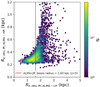 |
Fig. 12. Comparison of 158 μm sizes between low (≈0.3′′) and high (≈0.01′′) resolution ALMA configuration set-up is shown above for z = 5, 6 sample. The high resolution (≈0.01′′) sizes is on y-axis with low resolution (≈0.3′′) sizes on x-axis. The line shows the average beam radius for the low-resolution observations. |
We also compared the ALMA low angular resolution (≈0.3′′) sizes to the recent CRISTAL survey (Mitsuhashi et al. 2024; Ikeda et al. 2025), observed at similar resolutions. We find that the dust continuum sizes around [C II] emission in CRISTAL galaxies matches well with our dust-continuum sizes from mock ALMA observations at same wavelengths and resolutions. CRISTAL sizes range from 0.6–2.44 kpc with a mean of 1.38 kpc at z = 4 − 6 whereas for similar redshift range mock ALMA sizes for FLARES range from 0.42–3.32 kpc (99th percentile). With the intrinsic sizes of galaxies in FLARES for the same mass and redshift range as CRISTAL galaxies being much lower (≈10 times) than the beam size of observations, while the observed sizes are comparable, we find it is probable that the beam effects are enlarging the core emission of galaxies; this is similar to the effect of PSF leading to inflated ALMA sizes at low angular resolutions.
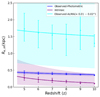 |
Fig. 13. Infrared size evolution with redshift at 50 um rest is shown with the half-light radius for both the simulations and mock-photometry on the y-axis and the redshift on the x-axis. The shaded areas highlight the error margins for the fit. |
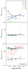 |
Fig. 14. Upper panel: Median intrinsic sizes(y-axis) of 50 μm in simulations as a function of stellar mass(x-axis) are shown. Middle panel: Evolution of mock IR photometric observational sizes at S/N =5. Lower panel: Evolution of ALMA observed sizes. The (≈0.01 − 0.02′′) angular resolution sizes are represented by the dotted lines and the low angular resolution (≈0.3′′) sizes are represented by the solid lines. The red scatter and the corresponding line show the CRISTAL Mitsuhashi et al. (2024) data and its best fit mass-size relation respectively. |
5.2. IR size evolution with redshift
We evaluated the evolution of sizes in the infrared with the same process used for UV. We calculate intrinsic sizes with the iterative aperture method and also use statmorph to calculate observed sizes for the photometric and ALMA imaging. Figure 13 shows the evolution of intrinsic and observed IR sizes, which follows a power law when the median sizes are plotted against redshift. There is negligible size evolution at IR wavelengths which leads to shallow slopes, with m = 0.24 for photometry, m = 0.16 for ALMA at low resolution and m = 1.39 for simulation size. FLARES galaxy cores were found to be heavily dust attenuated when radial dust attenuation was analysed in Vijayan et al. (2024). Our shallow slope values with intrinsic sizes being r ≤ 1 kpc also indicates that majority of the dust produced in the early universe is concentrated in compact cores. The observed IR size-evolution (Fig. 13) is also in agreement with ALMA observations of sub-millimetre galaxies (SMGs, Gullberg et al. 2019), showing a weak decline of dust-continuum sizes with increasing redshifts (up to z = 5.5). Further analysis with respect to comparison of sizes in IR against UV is discussed further in Sect. 6.2.
5.3. IR size evolution with stellar mass
To analyse the IR size evolution with stellar mass, we study their median evolution in bins of 0.5 dex stellar mass across each redshift. Figure 14 shows the evolution of intrinsic IR sizes with stellar mass. At M∗ ≥ 1010.0 M⊙, IR sizes exhibit a slight positive correlation with increasing mass. Figure 14 also shows the IR size evolution against stellar mass for photometric observations and ALMA low- and high-resolution observations respectively. The photometric sizes of galaxies show no significant evolution with increasing stellar mass and similar to UV, for same stellar mass, galaxies at lower redshift are larger in size. The ALMA low resolution sizes at fixed stellar mass are > 10 times the intrinsic sizes. It is important to note that at low ALMA resolution, a lot of the sample is unresolved. The median ALMA simulated sizes at ≈0.3′′ resolution lie well within the scatter of the CRISTAL data (Mitsuhashi et al. 2024). Compared to our simulated ALMA sizes, the best-fitting size-mass relation for CRISTAL shows a steeper positive evolution of size with increasing stellar mass; however, more observational data will be required at both the lower (M∗ ≤ 109.5 M⊙) and higher (M∗ ≥ 1010.5 M⊙) mass ends to get a robust infrared size-mass relation.
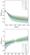 |
Fig. 15. Evolution of normalised size with rest-frame wavelength is shown in UV (upper panel) and IR (lower panel). The solid curves correspond to the median of the distribution, whereas the colour-shaded regions mark the one-sigma scatter of the distribution |
6. Panchromatic analysis
6.1. Size evolution with wavelengths
To evaluate the size evolution with wavelength, we first normalised the evolution by dividing the sizes by 1500 Å sizes for UV and 500 μm sizes for IR (intrinsic sizes). Figure 15 shows the evolution of median normalised sizes with increasing wavelengths. For each redshift, we observe a decrease (0.4 times the FUV size at 0.4 μm) in size with increasing wavelength. The size reduction is due to decreasing effect of dust attenuation with increasing wavelengths. At higher wavelengths weak attenuation results in bright centres which capture more luminosity in smaller apertures, reducing sizes effectively. This effect of dust attenuation decreasing with increasing wavelength has been analysed well in Marshall et al. (2022), FLARES IV, and our analysis in Appendix C.
Figure 15 also shows the evolution of median sizes at FIR wavelengths. These sizes are normalised, with sizes of 500 μm. For the FIR, which is not as affected by dust attenuation, we only see a slight positive trend in sizes with increasing wavelengths, which is due to the prevalence of hotter dust (probed by shorter wavelengths) in the centres. Popping et al. (2022), using the ILLUSTRIS-TNG 50 simulation, also showed a similar non-evolution of sizes (normalised at 850 μm in the observed-frame) with increasing wavelength in the IR.
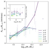 |
Fig. 16. Ratio of intrinsic sizes (main figure) as well mock observations (inset figure) at 1500 Å with observations like ALMA configuration is shown for UV and IR spectrum in stellar mass bins of 0.5 dex, with median values plotted as data-points. The error bars denote the 16th and 84th percentile values. Only sufficiently populated bins (N > 20) have been used to plot the lines. |
6.2. Comparison of sizes in UV and IR
UV emission is pre-dominantly from young stars within galaxies, hence size evolution in UV spectrum is indicative of the progression of unobscured star formation. IR emission helps us to understand the distribution of dust, and compared the UV sizes, IR sizes show shallow evolution either over time or with increasing stellar mass (see Sects. 4.4 and 5.3). This is consistent with studies like Popping et al. (2022). The increasing ratio of UV/IR size with increasing mass (as seen in Fig. 16) is driven by inside-out growth of star formation, rather than an increase in the dust obscuration within the centres. To analyse this size evolution ratio in UV and IR, we also look at previous FLARES work to understand the evolution of star formation and the processes behind it.
Roper et al. (2023, hereafter FLARES IX) details the different physical mechanisms driving the formation and evolution of compact galaxies. The study presents the physics behind the formation of compact star forming cores in galaxies in the early universe. The star formation criteria in the FLARE (or EAGLE) simulation, imposes a critical gas density (Schaye 2004), which is inversely related to the gas phase metallicity, shown in Eq. (3):
![Mathematical equation: $$ \begin{aligned} n_{\rm H}^\star (Z)=\min \left[ 0.1\, {\mathrm{cm} ^{-3}} \left({\frac{Z}{0.002}}\right)^{-0.64}, 10\,{\mathrm{cm} ^{-3}} \right] ,\end{aligned} $$](/articles/aa/full_html/2025/04/aa52040-24/aa52040-24-eq9.gif) (3)
(3)
where nH⋆(Z) is the density threshold and Z is the gas metallicity.
The FLARES galaxies in the early Universe are metal-poor7 and, thus, the gas density required for star-formation in the simulation is very high. However, once star formation starts in these dense cores, they become very quickly enriched with metals, lowering the critical density for star-formation. This triggers a state of runaway star-formation from this dense gas, quickly enriching them with metals and dust. Thus, these dense regions suffer from very high dust attenuation (see Fig. 2 in Vijayan et al. 2024). At later times the outer regions get enriched with metals, star formation is extended to the outer regions, which also leads to larger sizes in the UV. More details of these processes can be found in FLARES IX.
FLARES IX indicate that massive compact galaxies can form following two different evolution paths. It shows that galaxies at z = 5 can have progenitors that formed at z > 10 in pristine environments with low metal enrichment. Stars in such progenitors are formed at high densities and these galaxies remain compact throughout their evolution unaffected by mergers due to how compact they are (analysed in Appendix A of FLARES IX). The other path shows that galaxies can also transition from being diffused to compact. These galaxies have partially metal enriched progenitors (at z < 10) and have diffused star formation at lower gas densities. They become compact at lower redshifts (z < 6) when efficient cooling of gas happens in a diffused region, reaching high gas densities. This enables highly localised efficient star formation which enriches the gas in the core of the galaxy, leading to runaway star formation in the core. Hence, at z = 5 galaxies with stellar mass in range of 108.8 M⊙ ≤ M∗ ≤ 109.8 M⊙ show a significant decrease in size compared to z = 6 (see Fig. 6 in FLARES IX). Galaxies with stellar masses below this range (M∗ ≤ 108.8 M⊙) remain diffused clumpy systems and do not undergo a transition in size.
Figure 16 shows the UV/IR size ratio as a function of redshift for both radiative transfer sizes with no observational effects as well as mock observations for JWST and ALMA. We can see that for intrinsic sizes for the stellar masses in range 109.0 M⊙ ≤ M∗ ≤ 1010.0 M⊙, there is a sharp dip in ratio for z = 5 which can be attributed to galaxies in stellar mass range 108.8 M⊙ ≤ M∗ ≤ 109.8 M⊙ showing a median decrease in size due to transition from diffused to clumpy systems as presented in FLARES IX. But when the mock observations for ALMA (low angular resolution similar to Mitsuhashi et al. (2024), ≈0.3′′) and JWST are used, the ratio are significantly lower, and IR sizes can be larger than UV sizes, similar to what is seen in Pozzi et al. (2024), Fudamoto et al. (2022) and Mitsuhashi et al. (2024). UV/IR Size ratio curve for NIRCAM UV sizes and ALMA high angular resolution sizes, matches the intrinsic curve presented in Fig. 16 as with smaller beam, the ALMA sizes are predicted closer to the intrinsic IR sizes. A further spatial analysis between UV and IR will be presented in a future study.
7. Summary and conclusions
In this study, we performed a radiative transfer using SKIRT (Camps & Baes 2015, 2020) for galaxies from the FLARE simulations to study the size evolution in the UV and the far-IR at the EoR (z ∈ [5, 10]). Radiative transfer using Monte Carlo simulation allows us to precisely estimates the effect of dust absorption and scattering of radiation to provide a more accurate SED. We have used the results of the radiative transfer simulations to mock observations of these galaxies for NIRCam at the rest-frame FUV to find and analyse the offset in observational sizes to the intrinsic sizes of galaxies. We also simulated the imaging in the far-IR at wavelengths of 50 μm and 250 μm as well as interferometric observations by ALMA for the dust-continuum at 158 μm. The images are produced by taking into account the noise as well as the PSF (for mock imaging) or beam sizes (for ALMA configuration in CASA). We analysed our galaxies for various S/N values of ∈[5, 20]. To evaluate the sizes of galaxies in the simulation, after the radiative transfer, we used a curve of growth method, by using circular apertures of increasing radius from the most bound particle and interpolating the radius which encloses 50 per cent of the light. We used statmorph (Rodriguez-Gomez et al. 2019) to evaluate the sizes from the mock observations. Using both these methods, we were able to compare the sizes of mock observations with intrinsic sizes. Using these methods, we also calculated the sizes in IR regime.
We compared the slope parameter in the power laws (Eqs. (1) and (2)) of size evolution with cosmic time, as well as the size evolution against luminosity at fixed redshift, for both simulations and observations. We also analyse how the sizes vary with increasing mass and wavelength of observations in both UV and IR. Our main findings from these studies are as follows:
-
1.
Mock NIRCam observations of FLARES galaxies at rest frame FUV (1500 Å) show a decreasing size evolution with redshift, which is consistent with many observational studies. For the observed sizes, all our sample lies within the range of m = 1.0 − 2.0, as predicted in Ma et al. (2018). Our samples are in agreement with observational studies at both low luminosities (Oesch et al. 2010; Shibuya et al. 2015; Ono et al. 2013; Kawamata et al. 2018) and high luminosities (Holwerda et al. 2015). Our intrinsic size match the trends of dust attenuated size evolution in different luminosity bins, as presented in FLARES IV.
-
2.
For fixed redshifts, the size-luminosity evolution of the mock observations are in agreement with the studies of Shibuya et al. (2015), Holwerda et al. (2015), Grazian et al. (2012) and Bouwens et al. (2022) showing a positive β ≈ 0.27 (at z = 7). The slopes are also consistent with previous dust-attenuated simulation studies (FLARES IV, Marshall et al. 2022). Mock observed slopes are slightly shallower compared to early JWST (Yang et al. 2022) rest-frame UV size-luminosity slopes from F150W filter. However, at z > 6, we were able to match the size-luminosity scatter from the recent JWST surveys well. We also find a broadly non-evolving β with increasing redshift similar to Shibuya et al. (2015). The intrinsic size β which can recover the dispersed sample reports a β = 0.59.
-
3.
Due to observational effects of noise and PSF, at lower S/N, the mock observational sizes are underestimated. While at higher S/Ns, due to the reduced effect of noise sizes, have been underestimated at lower redshift (z = 5, 6, 7, 8) in NIRCam observations and at higher redshifts (z = 9, 10) the sizes tend to be slightly overestimated where the effect of PSF leads to bright cores becoming bigger. Hence, the ratio of mock observation sizes to intrinsic sizes is a function of the S/N.
-
4.
Mock photometric IR observations also show the effect of noise and PSF as the photometric sizes are underestimated compared to intrinsic sizes. For ALMA simulations at a high resolution with ALMA (≈0.01′′), the low-surface-brightness extended emissions of a galaxy will be lost leading to underestimation of sizes with a factor =0.89 times intrinsic size. Our sizes and achieved S/Ns for the ALMA low angular resolution (≈0.3′′) are a good match with the recent studies Mitsuhashi et al. (2024), Ikeda et al. (2025). Due to beam effects, the observed low angular resolution sizes are nearly ten times the intrinsic size of the galaxy. Nearly 50 per cent of the galaxy at this resolution fall below the beam size. Low S/N noise near the signal in these low-resolution ALMA observations (≈0.3′′) can also behave as extended emissions, hence, this may also lead to the sizes being extended further. The sizes in the IR spectrum follow the same power law as UVm but the sizes are substantially smaller for very high-resolution imaging. As the dust sizes remain compact at these redshift power laws are less steep with a slope of m = 0.24 for photometric observations, m = 0.16 for ALMA observations, and m = 1.39 for intrinsic sizes.
-
5.
The ratio of intrinsic sizes in UV and IR increases with increasing mass, which is due to higher mass galaxies having higher star formation rates and being dominated by young blue stars. Low-mass galaxies (log10(M∗/M⊙) ≈ 8.8 − 9.8) at z < 6 show a sudden dip in the UV-IR size ratio. This is due to the fact that this sample also contains galaxies transitioning from dispersed to compact star formation, as described in FLARES IX. The observed UV-IR size ratio (for simulated NIRCAM and ALMA imaging) shows dust sizes to be greater than UV sizes, which is in agreement with recent studies (Pozzi et al. 2024; Fudamoto et al. 2022; Mitsuhashi et al. 2024).
The variation of observed from intrinsic sizes highlights the importance of accounting for observational effects such as PSF and S/N when interpreting galaxy size measurements. As higher resolution photometry of galaxies in the EoR becomes increasingly available with JWST, the constraints on the size evolution slopes will become increasingly robust in UV. Observational effects such as S/N and angular resolution also affect the observed ALMA sizes. Studying sizes in IR to a high level of accuracy will also require very high-resolution observations, which would be able to resolve both small scale structures and low surface brightness extended emissions. Combining multi-wavelength studies of galaxy sizes in IR and UV can help us unravel the physics beneath dust-obscured star formation to understand the interplay of star formation, chemical enrichment, and feedback.
A proper comparison between observations and theory is now paramount to validating and refining our understanding of galaxy evolution. Next-generation simulations must aim to not only reproduce the UV luminosity functions, but also predict the observed size and luminosity distribution of galaxies across different observed wavelengths. In the upcoming future, new instruments such as Extremely Large Telescope (ELT) and Very Large Array (VLA) will be delivering valuable data to support advanced studies in this field. Investigations of the morphology and size evolution of high-redshift galaxies will be made possible by the unmatched spatial resolution and sensitivity that ELT and VLA will offer in the optical, infrared, and radio wavelengths. Square Kilometre Array (SKA) will also enable studies of the cold gas reservoirs and large-scale structures around these galaxies, allowing for the analysis of environmental factors behind galaxy growth. Together, these instruments will help develop a comprehensive, multi-wavelength view of early galaxy evolution. Coupling these next-generation multi-wavelength observations with simulations will refine our knowledge of galaxy formation and evolution at the epoch of re-ionisation, providing us with deeper insights into the complex interplay of gas, dust, and radiation.
Data availability
The size analysis data and the code to reproduce the plots is available at https://github.com/paurush-p/FLARES_XVI_plots.
β used here is not equivalent to the UV spectral slope.
This corresponds to M1600 = −21.0 mag or Lν = 1029.03 erg s−1 Hz−1 Steidel et al. (1999).
This lies below the gravitational softening length (s = 2.66/(1 + z) pkpc) of the simulation. Note: as calculated later in Sect. 2.5, our UV intrinsic sizes lie above the softening length, but as IR sizes go below the softening length, they can be unreliable.
We ignored data bins that are not sufficiently populated (N < 20) in all our size-evolution analysis. This reduces the effect of viewing angles. Our sample selection also encompasses a wide range of environments. With galaxies being selected from different regions, they are statistically randomly sampled, avoiding the intrinsic alignment of galaxies in nearby environments, as seen in simulations such as EAGLE (Hill et al. 2022).
We use curve_fit (non-linear least-squares fitting), from scipy (Virtanen et al. 2020), to produce fits and the error are generated by the covariance matrix.
Wilkins et al. (2023a) shows that at z = 5,  for FLARES is well within the scatter and error-margin of recent observational estimates (Cullen et al. 2019; Calabrò et al. 2021). While the sample are still being built at z > 10, Wilkins et al. (2023b) states median gas phase metallicity of log10(Zg) ≈ − 3 at M∗/M⊙ ≈ 108, which increases to ≈ − 2.5 for galaxies with M∗/M⊙ ≥ 109. This matches recent observations (Hsiao et al. 2023; Curtis-Lake et al. 2023; Harikane et al. 2024; Schouws et al. 2024; Carniani et al. 2025). Future scope of better statistics at high z still remains.
Acknowledgments
This work has been performed using the Danish National Life Science Supercomputing Center, Computerome. This work also used the DiRAC@Durham facility managed by the Institute for Computational Cosmology on behalf of the STFC DiRAC HPC Facility (www.dirac.ac.uk). The equipment was funded by BEIS capital funding via STFC capital grants ST/K00042X/1, ST/P002293/1, ST/R002371/1 and ST/S002502/1, Durham University and STFC operations grant ST/R000832/1. DiRAC is part of the National e-Infrastructure. The Cosmic Dawn Center (DAWN) is funded by the Danish National Research Foundation under grant DNRF140. We also wish to acknowledge the following open source software packages used in the analysis: NUMPY (Harris et al. 2020), SCIPY (Virtanen et al. 2020), PANDAS (The pandas development team 2020), ASTROPY (Astropy Collaboration 2013, 2018, 2022), PILLOW (Murray et al. 2025), MATPLOTLIB (Hunter 2007) and STATMORPH (Rodriguez-Gomez et al. 2019). PP would also like to thank Dr. Anurag Nishad and Dr. Anupama Sharma for guidance towards completion of his thesis leading to this study. The FLARES team would like to acknowledge the enormous contributions of the late Prof. Peter Thomas to the FLARES project; we will miss his guidance and great wit. We also thank the anonymous referee for their helpful comments.
References
- Astropy Collaboration (Robitaille, T. P., et al.) 2013, A&A, 558, A33 [NASA ADS] [CrossRef] [EDP Sciences] [Google Scholar]
- Astropy Collaboration (Price-Whelan, A. M., et al.) 2018, AJ, 156, 123 [Google Scholar]
- Astropy Collaboration (Price-Whelan, A. M., et al.) 2022, ApJ, 935, 167 [NASA ADS] [CrossRef] [Google Scholar]
- Behrens, C., Pallottini, A., Ferrara, A., Gallerani, S., & Vallini, L. 2018, MNRAS, 477, 552 [NASA ADS] [CrossRef] [Google Scholar]
- Bouwens, R. J., Illingworth, G. D., Blakeslee, J. P., Broadhurst, T. J., & Franx, M. 2004, ApJ, 611, L1 [Google Scholar]
- Bouwens, R. J., Illingworth, G. D., van Dokkum, P. G., et al. 2022, ApJ, 927, 81 [NASA ADS] [CrossRef] [Google Scholar]
- Bowler, R. A. A., Dunlop, J. S., McLure, R. J., & McLeod, D. J. 2017, MNRAS, 466, 3612 [NASA ADS] [CrossRef] [Google Scholar]
- Bowler, R. A. A., Cullen, F., McLure, R. J., Dunlop, J. S., & Avison, A. 2022, MNRAS, 510, 5088 [NASA ADS] [CrossRef] [Google Scholar]
- Bradley, L., Sipőcz, B., Robitaille, T., et al. 2023, https://doi.org/10.5281/zenodo.7946442 [Google Scholar]
- Calabrò, A., Castellano, M., Pentericci, L., et al. 2021, A&A, 646, A39 [EDP Sciences] [Google Scholar]
- Camps, P., & Baes, M. 2015, Astron. Comput., 9, 20 [Google Scholar]
- Camps, P., & Baes, M. 2020, Astron. Comput., 31, 100381 [NASA ADS] [CrossRef] [Google Scholar]
- Carniani, S., D’Eugenio, F., Ji, X., et al. 2025, A&A, 696, A87 [NASA ADS] [CrossRef] [EDP Sciences] [Google Scholar]
- CASA Team, Bean, B., Bhatnagar, S., et al. 2022, PASP, 134, 114501 [NASA ADS] [CrossRef] [Google Scholar]
- Chiang, Y.-K., Overzier, R., & Gebhardt, K. 2013, ApJ, 779, 127 [Google Scholar]
- Cochrane, R. K., Anglés-Alcázar, D., Cullen, F., & Hayward, C. C. 2024, ApJ, 961, 37 [NASA ADS] [CrossRef] [Google Scholar]
- Conroy, C., & Gunn, J. E. 2010, ApJ, 712, 833 [Google Scholar]
- Conselice, C. J. 2014, ARA&A, 52, 291 [CrossRef] [Google Scholar]
- Costantin, L., Pérez-González, P. G., Vega-Ferrero, J., et al. 2023, ApJ, 946, 71 [NASA ADS] [CrossRef] [Google Scholar]
- Crain, R. A., Schaye, J., Bower, R. G., et al. 2015, MNRAS, 450, 1937 [NASA ADS] [CrossRef] [Google Scholar]
- Cullen, F., McLure, R. J., Dunlop, J. S., et al. 2019, MNRAS, 487, 2038 [Google Scholar]
- Curtis-Lake, E., Carniani, S., Cameron, A., et al. 2023, Nat. Astron., 7, 622 [NASA ADS] [CrossRef] [Google Scholar]
- Davé, R., Anglés-Alcázar, D., Narayanan, D., et al. 2019, MNRAS, 486, 2827 [Google Scholar]
- Davis, M., Efstathiou, G., Frenk, C. S., & White, S. D. M. 1985, ApJ, 292, 371 [Google Scholar]
- Dolag, K., Borgani, S., Murante, G., & Springel, V. 2009, MNRAS, 399, 497 [Google Scholar]
- Eisenstein, D. J., Willott, C., Alberts, S., et al. 2023, ApJS, submitted [arXiv:2306.02465] [Google Scholar]
- Feng, Y., Di-Matteo, T., Croft, R. A., et al. 2016, MNRAS, 455, 2778 [NASA ADS] [CrossRef] [Google Scholar]
- Ferguson, H. C., Dickinson, M., Giavalisco, M., et al. 2004, ApJ, 600, L107 [NASA ADS] [CrossRef] [Google Scholar]
- Ferreira, L., Conselice, C. J., Sazonova, E., et al. 2023, ApJ, 955, 94 [NASA ADS] [CrossRef] [Google Scholar]
- Franx, M., van Dokkum, P. G., Förster Schreiber, N. M., et al. 2008, ApJ, 688, 770 [NASA ADS] [CrossRef] [Google Scholar]
- Fudamoto, Y., Smit, R., Bowler, R. A. A., et al. 2022, ApJ, 934, 144 [NASA ADS] [CrossRef] [Google Scholar]
- Grazian, A., Castellano, M., Fontana, A., et al. 2012, A&A, 547, A51 [NASA ADS] [CrossRef] [EDP Sciences] [Google Scholar]
- Groves, B., Dopita, M. A., Sutherland, R. S., et al. 2008, ApJS, 176, 438 [NASA ADS] [CrossRef] [Google Scholar]
- Gullberg, B., Smail, I., Swinbank, A. M., et al. 2019, MNRAS, 490, 4956 [Google Scholar]
- Harikane, Y., Nakajima, K., Ouchi, M., et al. 2024, ApJ, 960, 56 [NASA ADS] [CrossRef] [Google Scholar]
- Harris, C. R., Millman, K. J., van der Walt, S. J., et al. 2020, Nature, 585, 357 [NASA ADS] [CrossRef] [Google Scholar]
- Hill, A. D., Crain, R. A., McCarthy, I. G., & Brown, S. T. 2022, MNRAS, 511, 3844 [Google Scholar]
- Högbom, J. A. 1974, A&AS, 15, 417 [Google Scholar]
- Holwerda, B. W., Bouwens, R., Oesch, P., et al. 2015, ApJ, 808, 6 [CrossRef] [Google Scholar]
- Holwerda, B. W., Hsu, C.-C., Hathi, N., et al. 2024, MNRAS, 529, 1067 [NASA ADS] [CrossRef] [Google Scholar]
- Hsiao, T. Y.-Y., Coe, D., Abdurro’uf, et al. 2023, ApJ, 949, L34 [NASA ADS] [CrossRef] [Google Scholar]
- Huang, K.-H., Ferguson, H. C., Ravindranath, S., & Su, J. 2013, ApJ, 765, 68 [Google Scholar]
- Hunter, J. D. 2007, Comput. Sci. Eng., 9, 90 [NASA ADS] [CrossRef] [Google Scholar]
- Ikeda, R., Tadaki, K.-I., Mitsuhashi, I., et al. 2025, A&A, 693, A237 [NASA ADS] [CrossRef] [EDP Sciences] [Google Scholar]
- Jiang, L., Egami, E., Fan, X., et al. 2013, ApJ, 773, 153 [NASA ADS] [CrossRef] [Google Scholar]
- Kawamata, R., Ishigaki, M., Shimasaku, K., Oguri, M., & Ouchi, M. 2015, ApJ, 804, 103 [Google Scholar]
- Kawamata, R., Ishigaki, M., Shimasaku, K., et al. 2018, ApJ, 855, 4 [NASA ADS] [CrossRef] [Google Scholar]
- Kroupa, P. 2002, Science, 295, 82 [Google Scholar]
- LaChance, P., Croft, R., Ni, Y., et al. 2024, Open J. Astrophys., 8, 20 [Google Scholar]
- Leitherer, C., Schaerer, D., Goldader, J. D., et al. 1999, ApJS, 123, 3 [Google Scholar]
- Li, A. 2009, Optical Properties of Dust (Berlin, Heidelberg: Springer), 1 [Google Scholar]
- Li, Q., Narayanan, D., & Davé, R. 2019, MNRAS, 490, 1425 [CrossRef] [Google Scholar]
- Liang, L., Feldmann, R., Kereš, D., et al. 2019, MNRAS, 489, 1397 [NASA ADS] [CrossRef] [Google Scholar]
- Liu, C., Mutch, S. J., Poole, G. B., et al. 2017, MNRAS, 465, 3134 [Google Scholar]
- Lovell, C. C., Thomas, P. A., & Wilkins, S. M. 2018, MNRAS, 474, 4612 [NASA ADS] [CrossRef] [Google Scholar]
- Lovell, C. C., Vijayan, A. P., Thomas, P. A., et al. 2021, MNRAS, 500, 2127 [Google Scholar]
- Ma, X., Hopkins, P. F., Boylan-Kolchin, M., et al. 2018, MNRAS, 477, 219 [Google Scholar]
- Ma, X., Hayward, C. C., Casey, C. M., et al. 2019, MNRAS, 487, 1844 [NASA ADS] [CrossRef] [Google Scholar]
- Magnelli, B., Boogaard, L., Decarli, R., et al. 2020, ApJ, 892, 66 [NASA ADS] [CrossRef] [Google Scholar]
- Markov, V., Gallerani, S., Ferrara, A., et al. 2025, Nat. Astron., 9, 458 [Google Scholar]
- Marshall, M. A., Mutch, S. J., Qin, Y., Poole, G. B., & Wyithe, J. S. B. 2019, MNRAS, 488, 1941 [Google Scholar]
- Marshall, M. A., Wilkins, S., Di Matteo, T., et al. 2022, MNRAS, 511, 5475 [Google Scholar]
- Mitsuhashi, I., Tadaki, K.-I., Ikeda, R., et al. 2024, A&A, 690, A197 [NASA ADS] [CrossRef] [EDP Sciences] [Google Scholar]
- Mo, H. J., & White, S. D. M. 2002, MNRAS, 336, 112 [Google Scholar]
- Mo, H. J., Mao, S., & White, S. D. M. 1998, MNRAS, 295, 319 [Google Scholar]
- Morishita, T., Stiavelli, M., Chary, R.-R., et al. 2024, ApJ, 963, 9 [NASA ADS] [CrossRef] [Google Scholar]
- Mosleh, M., Williams, R. J., Franx, M., et al. 2012, ApJ, 756, L12 [NASA ADS] [CrossRef] [Google Scholar]
- Murray, A., Kemenade, H. V., Clark, J. A., et al. 2025, https://doi.org/10.5281/zenodo.14586647 [Google Scholar]
- Nelson, D., Pillepich, A., Springel, V., et al. 2019, MNRAS, 490, 3234 [Google Scholar]
- Oesch, P. A., Bouwens, R. J., Carollo, C. M., et al. 2010, ApJ, 709, L21 [NASA ADS] [CrossRef] [Google Scholar]
- Ono, Y., Ouchi, M., Curtis-Lake, E., et al. 2013, ApJ, 777, 155 [NASA ADS] [CrossRef] [Google Scholar]
- Ormerod, K., Conselice, C. J., Adams, N. J., et al. 2024, MNRAS, 527, 6110 [Google Scholar]
- Perrin, M. D., Soummer, R., Elliott, E. M., Lallo, M. D., & Sivaramakrishnan, A. 2012, in Space Telescopes and Instrumentation 2012: Optical, Infrared, and Millimeter Wave, eds. M. C. Clampin, G. G. Fazio, H. A. MacEwen, J. Oschmann, & M. Jacobus, SPIE Conf. Ser., 8442, 84423D [Google Scholar]
- Perrin, M. D., Sivaramakrishnan, A., Lajoie, C.-P., et al. 2014, in Space Telescopes and Instrumentation 2014: Optical, Infrared, and Millimeter Wave, eds. J. Oschmann, M. Jacobus, M. Clampin, G. G. Fazio,&H. A. MacEwen, SPIE Conf. Ser., 9143, 91433X [CrossRef] [Google Scholar]
- Pillepich, A., Nelson, D., Springel, V., et al. 2019, MNRAS, 490, 3196 [Google Scholar]
- Popping, G., Pillepich, A., Calistro Rivera, G., et al. 2022, MNRAS, 510, 3321 [CrossRef] [Google Scholar]
- Pozzi, F., Calura, F., Fudamoto, Y., et al. 2021, A&A, 653, A84 [NASA ADS] [CrossRef] [EDP Sciences] [Google Scholar]
- Pozzi, F., Calura, F., D’Amato, Q., et al. 2024, A&A, 686, A187 [NASA ADS] [CrossRef] [EDP Sciences] [Google Scholar]
- Rodriguez-Gomez, V., Snyder, G. F., Lotz, J. M., et al. 2019, MNRAS, 483, 4140 [NASA ADS] [CrossRef] [Google Scholar]
- Roper, W. J., Lovell, C. C., Vijayan, A. P., et al. 2022, MNRAS, 514, 1921 [NASA ADS] [CrossRef] [Google Scholar]
- Roper, W. J., Lovell, C. C., Vijayan, A. P., et al. 2023, MNRAS, 526, 6128 [NASA ADS] [CrossRef] [Google Scholar]
- Schaye, J. 2004, ApJ, 609, 667 [NASA ADS] [CrossRef] [Google Scholar]
- Schaye, J., Crain, R. A., Bower, R. G., et al. 2015, MNRAS, 446, 521 [Google Scholar]
- Schouws, S., Bouwens, R. J., Ormerod, K., et al. 2024, ApJ, accepted [arXiv:2409.20549] [Google Scholar]
- Sérsic, J. L. 1963, Boletin de la Asociacion Argentina de Astronomia La Plata Argentina, 6, 41 [Google Scholar]
- Shen, X., Vogelsberger, M., Borrow, J., et al. 2024, MNRAS, 534, 1433 [Google Scholar]
- Shibuya, T., Ouchi, M., & Harikane, Y. 2015, ApJS, 219, 15 [Google Scholar]
- Shivaei, I., Alberts, S., Florian, M., et al. 2024, A&A, 690, A89 [NASA ADS] [CrossRef] [EDP Sciences] [Google Scholar]
- Springel, V., White, S. D. M., Tormen, G., & Kauffmann, G. 2001, MNRAS, 328, 726 [Google Scholar]
- Springel, V., White, S. D. M., Jenkins, A., et al. 2005, Nature, 435, 629 [Google Scholar]
- Stanway, E. R., & Eldridge, J. J. 2018, MNRAS, 479, 75 [NASA ADS] [CrossRef] [Google Scholar]
- Steidel, C. C., Adelberger, K. L., Giavalisco, M., Dickinson, M., & Pettini, M. 1999, ApJ, 519, 1 [NASA ADS] [CrossRef] [Google Scholar]
- Steinacker, J., Baes, M., & Gordon, K. D. 2013, ARA&A, 51, 63 [CrossRef] [Google Scholar]
- Stetson, P. B. 1990, PASP, 102, 932 [Google Scholar]
- The pandas development team 2020, https://doi.org/10.5281/zenodo.3509134 [Google Scholar]
- Varadaraj, R. G., Bowler, R. A. A., Jarvis, M. J., et al. 2024, MNRAS, 533, 3724 [Google Scholar]
- Vijayan, A. P., Clay, S. J., Thomas, P. A., et al. 2019, MNRAS, 489, 4072 [NASA ADS] [CrossRef] [Google Scholar]
- Vijayan, A. P., Lovell, C. C., Wilkins, S. M., et al. 2021, MNRAS, 501, 3289 [NASA ADS] [Google Scholar]
- Vijayan, A. P., Wilkins, S. M., Lovell, C. C., et al. 2022, MNRAS, 511, 4999 [NASA ADS] [CrossRef] [Google Scholar]
- Vijayan, A. P., Thomas, P. A., Lovell, C. C., et al. 2024, MNRAS, 527, 7337 [Google Scholar]
- Virtanen, P., Gommers, R., Oliphant, T. E., et al. 2020, Nat. Methods, 17, 261 [Google Scholar]
- Ward, E., de la Vega, A., Mobasher, B., et al. 2024, ApJ, 962, 176 [NASA ADS] [CrossRef] [Google Scholar]
- Weingartner, J. C., & Draine, B. T. 2001, ApJ, 548, 296 [Google Scholar]
- Wilkins, S. M., Vijayan, A. P., Lovell, C. C., et al. 2023a, MNRAS, 518, 3935 [Google Scholar]
- Wilkins, S. M., Vijayan, A. P., Lovell, C. C., et al. 2023b, MNRAS, 519, 3118 [Google Scholar]
- Witstok, J., Shivaei, I., Smit, R., et al. 2023, Nature, 621, 267 [CrossRef] [Google Scholar]
- Wu, X., Davé, R., Tacchella, S., & Lotz, J. 2020, MNRAS, 494, 5636 [Google Scholar]
- Xie, Y., Li, A., & Hao, L. 2017, ApJS, 228, 6 [Google Scholar]
- Yang, L., Morishita, T., Leethochawalit, N., et al. 2022, ApJ, 938, L17 [NASA ADS] [CrossRef] [Google Scholar]
- Yates, R. M., Hendriks, D., Vijayan, A. P., et al. 2024, MNRAS, 527, 6292 [Google Scholar]
Appendix A: Size calculation convergence test
As described in the text, we have used two separate methods to calculate intrinsic galaxy sizes and observed sizes. Hence, we tested the convergence of sizes using both methods on noise and PSF free radiative transfer output. We created a subsample consisting of 626 galaxies which follow the same relative distribution of galaxy stellar mass and redshift as in the larger sample. We then calculated sizes using statmorph while removing cases of segmentation failure from the sample. The resulting size relation is presented in Fig. A.1
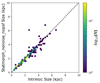 |
Fig. A.1. Plot of the sizes calculated by statmorph for noise and PSF free radiative transfer output on y-axis and the respective intrinsic sizes calculated by the Iterative Aperture Method on the x-axis. The black dotted line represents the 1:1 relation with the colourbar showing the number density in the hexbins. |
Appendix B: NIRCam calculated resolutions
The resolution used for NIRCam based on filters and redshift, calculated by (Astropy Collaboration 2013, 2018, 2022) is presented in Table B.1.
NIRCam Image Resolution at different redshifts for a field of view of 60 pkpcx60 pkpc (size of radiative transfer simulations)
The radiative transfer outputs are regridded to these resolutions for mocking observations.
Appendix C: Effect of dust on luminosity
To evaluate the evolution of attenuation effect of dust with wavelength we fit the size-luminosity relation at z=7 at 1500 Å, 2000 Å, 3000 Å and 4000 Å for the intrinsic non parametric sizes as defined in Sect. 2.5 in Fig. C.1. We used non-parametric sizes to prevent any clumpy or dispersed morphological shapes from affecting the size-luminosity fits. This allowed us to probe the effect of dust independently. As the attenuation effect of dust weakens with increasing wavelength, we see that at a fixed redshift the slopes of the luminosity size fit decreases.
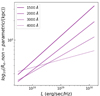 |
Fig. C.1. Intrinsic non-parametric sizes (y-axis) are fit for the size luminosity relation at z=7 for 1500 Å, 2000 Å, 3000 Å and 4000 Å respectively, which is plotted against the luminosities at the respective wavelengths (x-axis). The slopes decrease with increasing wavelength. |
Appendix D: Size-offset relation to galaxy characteristics
To determine why there is an offset between observational sizes and intrinsic sizes, in Fig. D.1, we plot the ratio of sizes in simulations to observational size on a plane of FUV luminosity and stellar mass, seeing no significant correlation.
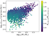 |
Fig. D.1. Ratio of simulation to observational sizes is plotted in the plane of stellar mass (x-axis) and FUV luminosity (y-axis) for galaxies at z=5 |
Appendix E: Effect of noise and PSF on r20 and r80
We analysed how the relative distribution of light for the galaxies changes due to observational effect. Figure E.1 evaluates r20 & r80 of galaxies with size underestimation at S/N=5 and overestimation at S/N=20 for intrinsic and observed imaging. All sizes are normalised by the half-light radius for that specific imaging. When underestimation takes place at low S/N, the observed r20 shows a subsequent increase signifying that low luminous regions blend with noise leading to a loss in luminosity that is not recovered by the PSF enlargement of the cores. This is compensated for by the decrease in observed r80. At high S/N, the loss in luminosity by noise is lower and this can also be recovered by the PSF’s enlargement of bright cores. This relative shift of luminosity to the centre leads to only a slight increase in observed r80, with the observed r20 being close to the intrinsic r20.
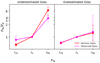 |
Fig. E.1. Ratio of r20 and r80 with the half-light radius (y-axis) are plotted for galaxies with underestimated sizes at S/N=5 and overestimated sizes at S/N=20. |
Appendix F: Simulated observations in a singular noise field
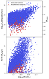 |
Fig. F.1. Upper panel: FUV luminosities (y-axis) are plotted against their respective Stellar Masses (x-axis). Detected galaxies are shown in blue and non-detections in red, at S/N=5. The scatter is of the whole sample across all redshifts with most non-detections lying at z=5,6. Lower Panel: Similar figure as the upper panel, we now compare SFR (y-axis) of the galaxies detected using mock images and the ones which were not at different stellar masses (x-axis) at S/N=5. Detected galaxies are shown in blue and non-detections in red. |
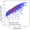 |
Fig. F.2. IR luminosity at 250 μm (y-axis) is plotted against Stellar Mass (x-axis) for the whole population to distinguish the IR properties between FUV-detected galaxies against the non-detected ones. The non-detections show a similar spread and pattern to detections. |
We analysed the galaxies when they are placed in a singular noise field to analyse the effect of same observation time on detection and non-detection. We found that out of a total sample of 6890 galaxies 167 will not be detected at 1500 Å by JWST. The galaxies which are not detected have low luminosities compared to the galaxies which were detected for similar stellar mass (see Fig. F.1). On further visual inspection of the galaxy images, we see that these galaxies are very dispersed and hence at lower S/N, a lot of the detail in these galaxies falls below the noise depth. These galaxies also have a comparatively lower SFR (see Fig. F.1) to the rest of the data-set. The IR sizes of these galaxies are compact and similar to other galaxies which are detected. The infrared characteristics as well as example images of these galaxies is discussed in Appendix.
The galaxies which are not detected in UV spectrum, as discussed earlier, have a comparatively lower SFR compared to the general population and they have a low luminosity detected at 1500 Å, but these galaxies have similar luminosities (to general population) in IR, signifying an older stellar population, which is also responsible for the stellar mass being comparable to the general population.
We also looked at the IRX-β plot to see if this non-detection can also be due to presence of dust but the galaxies which are not detected are spread across a wide value of IRX and β.
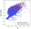 |
Fig. F.3. IRX (y-axis) - β (x-axis) is plotted for the whole sample to investigate the effect of dust between FUV detected galaxies against the non-detected ones. No clear pattern for non-detections is established to allude to dust causing non-detections. |
A few sample images of these non-detected galaxies with the original, noisy image and then the resultant image when a 5 σ noise threshold is applied are given in Fig. F.4.
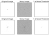 |
Fig. F.4. Sample non-detections of galaxies at various stages of image analysis are shown above. The first panel shows the output of radiative transfer, the second panel shows the simulated noisy image with respect to NIRCam and the last panel shows the residual image obtained after a 5-sigma threshold is applied to remove noise. The final images lead to segmentation algorithm finding no credible sources. |
Appendix G: Effect of noise on ALMA imaging
At low S/N in ALMA with very low resolution, noise around the bright centres of galaxies can appear as extended emission. To analyse this effect, in Fig. G.1 we plotted the 158μm observed to intrinsic size ratio against observed S/N levels. We see that with decreasing S/N the spread of the size ratio increases towards higher values. This effect is opposite of what is seen for UV emission where the decreasing effect of noise leads to mock JWST sizes getting closer to intrinsic sizes.
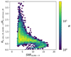 |
Fig. G.1. Observed to intrinsic size ratios at 158 μm (y-axis) plotted against the observed S/N (x-axis). The spread of galaxies towards higher size ratios increases with decreasing S/N. |
Appendix H: Mock high angular resolution ALMA imaging
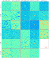 |
Fig. H.1. Sample galaxies (same galaxies as in Fig. 4) at different redshifts and various mass bins as observed by ALMA at 158 μm at very high resolution (≈0.02′′) using C8 configuration. The aperture of the images is 10 pkpc. The beam size is shown by the circle at the bottom-left corner |
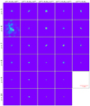 |
Fig. H.2. Radiative transfer output at 158 μm of the sample galaxies (same galaxies as in Fig. 4). The aperture of the images is 10 pkpc. |
Theoretically ALMA can go to very high resolutions, even beyond JWST resolutions, at a lot of galaxy structures will be resolved. The observational time required to achieve these resolutions on a single source remains unjustifiable, but to look at the effects of resolution on ALMA sizes we simulated galaxies’ observations with C8 configuration as described in main text. The imaging is presented in Fig. H.1.
Appendix I: Size-luminosity relation comparison
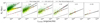 |
Fig. I.1. Non-weighted luminosity size relation evaluated at different redshifts is shown above. The y-axis shows the UV 1500 Å sizes in kpc and the x-axis shows luminosity at the same wavelength. The green scatter shows our sample of galaxies analysed with radiative transfer for curves of growth sizes using circular apertures whereas the yellow scatter shows the sizes for non-parametric Pixel Method as presented in FLARES IV. |
To show the effect of using a non-parametric pixel based method as presented in FLARES IV to this studies’ curves of growth method we fit the size luminosity relation for both size calculation methods to the radiative transfer output in Fig. I.1.
Appendix J: Size overestimation effect of PSF
To understand the effect of PSF independent of noise we also simulated UV 1500 Å imaging without effect of PSF but Gaussian noise included. We did this at S/N=15 as mock images with full observational effects show both underestimation and overestimation for this sample. We also removed any galaxy with greater than 5 segments detected, to avoid extremely clumpy systems as these clumps without the effect of PSF will be extremely small and isolated. The comparison of intrinsic sizes to the no-PSF imaging sizes is present in Fig. J.1. We see that at all redshifts most of the observed sample is underestimated in size with factors of 0.48-0.53 times the intrinsic size. For imaging with PSF as shown in Table 4 the underestimation is seen to reduce from 0.64 times at z=5 to 0.83 times at z=8 and then overestimation takes place with sizes being 1.04-1.07 times intrinsic sizes at z=9, 10. It is clear that PSF causes overestimation or restricts underestimation of sizes due to noise. As the PSF spreads light from bright sources, sizes of more compact systems should be affected by this spread more than dispersed systems. In Fig. J.2 we plotted the ratio of intrinsic and observed sizes against the intrinsic sizes and found that the more compact a galaxy is the less underestimated its observed sizes will be and can even be overestimated.
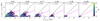 |
Fig. J.1. Observed UV sizes with no PSF effect from mock images (y-axis) are plotted as a function of intrinsic sizes (x-axis) at S/N=15. The black dashed line is a 1:1 relation whereas the magenta line is the best fit y=mx relation where y is mock image effective radius and x is simulation effective radius |
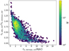 |
Fig. J.2. Observed-to-intrinsic UV size ratio (y-axis) plotted against the intrinsic sizes (x-axis) at S/N=5 and z=5. |
Appendix K: Very high S/N UV imaging
To further verify our overestimation being the effect of observational effects, in Fig. K.1 we plotted the relation between intrinsic and galaxies at S/N=50 and S/N=100 with the PSF applied. As the effect of noise becomes minimal at eating away at the faint parts of the galaxy, we see an overestimation of size at all redshifts. In Fig. K.2 we also plotted the Stellar mass-size relation at these S/Ns, seeing the evolution of sizes following the same positive trend as intrinsic-size relation.
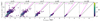 |
Fig. K.1. Observed UV sizes at S/N=100 mock images (y-axis) are plotted as a function of intrinsic sizes (x-axis). The black dashed line is a 1:1 relation, whereas the magenta line is the best fit y=mx relation where y is the mock image’s effective radius and x is the simulation’s effective radius |
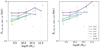 |
Fig. K.2. Left panel: Evolution of the mock observation sizes at S/N=50 (y- axis, in kpc) as function of stellar mass (x-axis) for z ∈ [5, 10]. Right panel: Evolution of sizes from mock observations at S/N=100 as function of stellar mass. |
All Tables
Mean percentage of pixels is shown in each relative brightness bins after normalising the intrinsic images in a square aperture of width equal to 4Re (Re is intrinsic RT size).
Mean percentage of pixels is shown in each relative brightness bins after normalising the observed (S/N =5) images in a square aperture of width equal to 4Re (Re is intrinsic RT size).
Slopes of the best-fit lines (y = mx, no intercept), where y is the mock image’s effective radius and x is the simulation’s effective radius at different S/Ns.
β at different redshifts for radiative transfer output and the mock images (S/N =15) created.
NIRCam Image Resolution at different redshifts for a field of view of 60 pkpcx60 pkpc (size of radiative transfer simulations)
All Figures
|
Fig. 1. Luminosity from SKIRT radiative transfer (estimated at 1500 Å) on x axis is compared with LoS luminosities (as discussed in Vijayan et al. 2021) on y axis. Luminosity from the LoS method is roughly 0.25–0.3 dex higher than luminosities produced by radiative transfer. The red line is the best fit offset between the two luminosities. The colours corresponding to the colourbar shows the average stellar mass in each hexbin. |
| In the text | |
|
Fig. 2. Comparison of the half-light radii at 1500 Å using the method from FLARES IV and this studies’ circular aperture method is shown above. The calculated HLR from a non-parametric pixel-based method is plotted on the y-axis with the intrinsic sizes plotted on the x-axis. Sizes from non-parametric pixel method are lower than intrinsic sizes used in this study due to non-parametric pixel method accounting for the most compact configuration of the galaxy. The green line shows the 1:1 relation. |
| In the text | |
|
Fig. 3. Sample galaxy image at z = 5 at various stages of methodology, in a 60 × 60 pkpc2 field of view. First panel: Result of SKIRT radiative transfer simulation. Second and third panels: Mock observation produced after regridding to 302 × 302 pixels based on Near Infrared Camera (NIRCam) resolution at this redshift and adding the effects of Gaussian + shot noise corresponding to S/N =5 and PSF is shown in the second panel with its respective segmentation map in the third panel showing only a single detected object. Fourth and fifth panels: Simulated imaging, as described earlier, but it is shown at S/N =15 in fourth panel, with its respective segmentation map and showing three distinct objects detected in the fifth panel. |
| In the text | |
|
Fig. 4. False colour images from the previous figure, here showing sample galaxies at different redshifts and various mass bins at S/N =20. The FoV of the images is 20 pkpc and the red, green, and blue channel taken from JWST/NIRCam F200W, F150W, and F115W filter data, respectively. |
| In the text | |
|
Fig. 5. Sample of galaxies (same galaxies as in Fig. 4) as observed by ALMA at 158 μm at an aperture of 30 pkpc. Low angular resolution (≈0.1′′) (similar to CRISTAL program) is used. The beam size is shown by the circle at bottom left corner. The black contours show four linearly spaced contours between brightest pixel to 1/4th of brightest pixel for 1500 Å. |
| In the text | |
|
Fig. 6. Brightness comparison between original and noisy image is shown for a sample redshift 5, 7 & 10 galaxies with size offset at S/N =5. The bottom row shows the mean luminosity of pixels at each radius (y-axis) calculated by finding pixel luminosities at the edge of the aperture and dividing it by circumference) plotted against the radius (x-axis) for the normalised images. The centre for these luminosities is assumed as the centre of potential as defined in the simulations. The red lines indicate the maximum brightness and the green line shows the median brightness. The blue solid and dashed lines show the r20 of original and noisy image respectively. The purple solid and dashed lines show the r80 of original and noisy images respectively. Panel for z = 5 shows the case of underestimation, z = 7 of near parity and z = 10 shows an overestimation. |
| In the text | |
|
Fig. 7. Observed UV sizes from mock images (y-axis) are plotted as a function of intrinsic sizes (x-axis) at S/N =5. The black dashed line is a 1:1 relation whereas the magenta line is the best fit y = mx relation where y is observed size and x is intrinsic size. |
| In the text | |
|
Fig. 8. UV luminosity size relation at different redshifts is shown. The y-axis shows the UV 1500 Å sizes in kpc and the x-axis shows luminosity at the same wavelength. The green scatter shows our sample of galaxies analysed with radiative transfer and then simulated observations for NIRCAM. The red plots show the median luminosity and sizes in bins of 0.3 dex in luminosity with 16th and 84th percentile error bars. The black line is an linear fit to the median luminosity and sizes fit to the power law. We also compare our sample with observational studies (Holwerda et al. 2015; Bouwens et al. 2022) and simulations (Marshall et al. 2022, FLARES IV). JWST data have been taken from Morishita et al. (2024) and Ormerod et al. (2024) for the sample with M∗/M⊙ ≥ 109 from the JADES (Eisenstein et al. 2023), CEERS (Holwerda et al. 2024), and PRIMER survey. |
| In the text | |
|
Fig. 9. Left: Comparison of the size-luminosity slopes (β) in relation with other studies (Roper et al. 2022; Liu et al. 2017; Marshall et al. 2022; Bouwens et al. 2022; Shibuya et al. 2015; Holwerda et al. 2015; Grazian et al. 2012) at z = 7 (blue shaded region are simulation studies) is shown. Right: Comparison of the UV size evolution slopes (m) in relation with other studies (Roper et al. 2022; Marshall et al. 2022; Oesch et al. 2010; Holwerda et al. 2015; Kawamata et al. 2018; Ono et al. 2013; Shibuya et al. 2015) is shown. |
| In the text | |
|
Fig. 10. Upper panel: Evolution of the UV simulation sizes (y-axis, in kpc) as function of stellar mass (x-axis) for z ∈ [5, 10]. Lower panel: Evolution of sizes from mock observations as function of stellar mass. Size mass relation for simulated observations from Costantin et al. (2023) and LaChance et al. (2024) and NIRCAM observations from Ward et al. (2024). CEERS data has been taken from Morishita et al. (2024) and Ormerod et al. (2024). |
| In the text | |
|
Fig. 11. Comparison of sizes between various IR observation methods is shown above. The plot compares IR sizes (y-axis) from mock photometry (50 μm) and ALMA simulations (high-resolution, ≈0.01 − 0.02′′ at 156 μm) with intrinsic sizes (50 μm) (x-axis). The hex-bin plot shows the log mapped distribution of photometric sizes whereas the contours show the log mapped distribution of mock ALMA sizes. The black line shows the 1:1 relation with the yellow line showing the best-fit y = mx relation. All ALMA sizes in this plot of high angular resolution (≈0.01′′ angular resolution). |
| In the text | |
|
Fig. 12. Comparison of 158 μm sizes between low (≈0.3′′) and high (≈0.01′′) resolution ALMA configuration set-up is shown above for z = 5, 6 sample. The high resolution (≈0.01′′) sizes is on y-axis with low resolution (≈0.3′′) sizes on x-axis. The line shows the average beam radius for the low-resolution observations. |
| In the text | |
|
Fig. 13. Infrared size evolution with redshift at 50 um rest is shown with the half-light radius for both the simulations and mock-photometry on the y-axis and the redshift on the x-axis. The shaded areas highlight the error margins for the fit. |
| In the text | |
|
Fig. 14. Upper panel: Median intrinsic sizes(y-axis) of 50 μm in simulations as a function of stellar mass(x-axis) are shown. Middle panel: Evolution of mock IR photometric observational sizes at S/N =5. Lower panel: Evolution of ALMA observed sizes. The (≈0.01 − 0.02′′) angular resolution sizes are represented by the dotted lines and the low angular resolution (≈0.3′′) sizes are represented by the solid lines. The red scatter and the corresponding line show the CRISTAL Mitsuhashi et al. (2024) data and its best fit mass-size relation respectively. |
| In the text | |
|
Fig. 15. Evolution of normalised size with rest-frame wavelength is shown in UV (upper panel) and IR (lower panel). The solid curves correspond to the median of the distribution, whereas the colour-shaded regions mark the one-sigma scatter of the distribution |
| In the text | |
|
Fig. 16. Ratio of intrinsic sizes (main figure) as well mock observations (inset figure) at 1500 Å with observations like ALMA configuration is shown for UV and IR spectrum in stellar mass bins of 0.5 dex, with median values plotted as data-points. The error bars denote the 16th and 84th percentile values. Only sufficiently populated bins (N > 20) have been used to plot the lines. |
| In the text | |
|
Fig. A.1. Plot of the sizes calculated by statmorph for noise and PSF free radiative transfer output on y-axis and the respective intrinsic sizes calculated by the Iterative Aperture Method on the x-axis. The black dotted line represents the 1:1 relation with the colourbar showing the number density in the hexbins. |
| In the text | |
|
Fig. C.1. Intrinsic non-parametric sizes (y-axis) are fit for the size luminosity relation at z=7 for 1500 Å, 2000 Å, 3000 Å and 4000 Å respectively, which is plotted against the luminosities at the respective wavelengths (x-axis). The slopes decrease with increasing wavelength. |
| In the text | |
|
Fig. D.1. Ratio of simulation to observational sizes is plotted in the plane of stellar mass (x-axis) and FUV luminosity (y-axis) for galaxies at z=5 |
| In the text | |
|
Fig. E.1. Ratio of r20 and r80 with the half-light radius (y-axis) are plotted for galaxies with underestimated sizes at S/N=5 and overestimated sizes at S/N=20. |
| In the text | |
|
Fig. F.1. Upper panel: FUV luminosities (y-axis) are plotted against their respective Stellar Masses (x-axis). Detected galaxies are shown in blue and non-detections in red, at S/N=5. The scatter is of the whole sample across all redshifts with most non-detections lying at z=5,6. Lower Panel: Similar figure as the upper panel, we now compare SFR (y-axis) of the galaxies detected using mock images and the ones which were not at different stellar masses (x-axis) at S/N=5. Detected galaxies are shown in blue and non-detections in red. |
| In the text | |
|
Fig. F.2. IR luminosity at 250 μm (y-axis) is plotted against Stellar Mass (x-axis) for the whole population to distinguish the IR properties between FUV-detected galaxies against the non-detected ones. The non-detections show a similar spread and pattern to detections. |
| In the text | |
|
Fig. F.3. IRX (y-axis) - β (x-axis) is plotted for the whole sample to investigate the effect of dust between FUV detected galaxies against the non-detected ones. No clear pattern for non-detections is established to allude to dust causing non-detections. |
| In the text | |
|
Fig. F.4. Sample non-detections of galaxies at various stages of image analysis are shown above. The first panel shows the output of radiative transfer, the second panel shows the simulated noisy image with respect to NIRCam and the last panel shows the residual image obtained after a 5-sigma threshold is applied to remove noise. The final images lead to segmentation algorithm finding no credible sources. |
| In the text | |
|
Fig. G.1. Observed to intrinsic size ratios at 158 μm (y-axis) plotted against the observed S/N (x-axis). The spread of galaxies towards higher size ratios increases with decreasing S/N. |
| In the text | |
|
Fig. H.1. Sample galaxies (same galaxies as in Fig. 4) at different redshifts and various mass bins as observed by ALMA at 158 μm at very high resolution (≈0.02′′) using C8 configuration. The aperture of the images is 10 pkpc. The beam size is shown by the circle at the bottom-left corner |
| In the text | |
|
Fig. H.2. Radiative transfer output at 158 μm of the sample galaxies (same galaxies as in Fig. 4). The aperture of the images is 10 pkpc. |
| In the text | |
|
Fig. I.1. Non-weighted luminosity size relation evaluated at different redshifts is shown above. The y-axis shows the UV 1500 Å sizes in kpc and the x-axis shows luminosity at the same wavelength. The green scatter shows our sample of galaxies analysed with radiative transfer for curves of growth sizes using circular apertures whereas the yellow scatter shows the sizes for non-parametric Pixel Method as presented in FLARES IV. |
| In the text | |
|
Fig. J.1. Observed UV sizes with no PSF effect from mock images (y-axis) are plotted as a function of intrinsic sizes (x-axis) at S/N=15. The black dashed line is a 1:1 relation whereas the magenta line is the best fit y=mx relation where y is mock image effective radius and x is simulation effective radius |
| In the text | |
|
Fig. J.2. Observed-to-intrinsic UV size ratio (y-axis) plotted against the intrinsic sizes (x-axis) at S/N=5 and z=5. |
| In the text | |
|
Fig. K.1. Observed UV sizes at S/N=100 mock images (y-axis) are plotted as a function of intrinsic sizes (x-axis). The black dashed line is a 1:1 relation, whereas the magenta line is the best fit y=mx relation where y is the mock image’s effective radius and x is the simulation’s effective radius |
| In the text | |
|
Fig. K.2. Left panel: Evolution of the mock observation sizes at S/N=50 (y- axis, in kpc) as function of stellar mass (x-axis) for z ∈ [5, 10]. Right panel: Evolution of sizes from mock observations at S/N=100 as function of stellar mass. |
| In the text | |
Current usage metrics show cumulative count of Article Views (full-text article views including HTML views, PDF and ePub downloads, according to the available data) and Abstracts Views on Vision4Press platform.
Data correspond to usage on the plateform after 2015. The current usage metrics is available 48-96 hours after online publication and is updated daily on week days.
Initial download of the metrics may take a while.