| Issue |
A&A
Volume 698, June 2025
|
|
|---|---|---|
| Article Number | A30 | |
| Number of page(s) | 14 | |
| Section | Extragalactic astronomy | |
| DOI | https://doi.org/10.1051/0004-6361/202452690 | |
| Published online | 23 May 2025 | |
Galaxy size and mass build-up in the first 2 Gyr of cosmic history from multi-wavelength JWST NIRCam imaging
1
Cosmic Dawn Centre (DAWN), Copenhagen, Denmark
2
Niels Bohr Institute, University of Copenhagen, Jagtvej 128, DK-2200 Copenhagen N, Denmark
3
Department of Astronomy, University of Geneva, Chemin Pegasi 51, 1290 Versoix, Switzerland
4
Jodrell Bank Centre for Astrophysics, University of Manchester, Oxford Road, Manchester M13 9PL, UK
5
DTU-Space, Elektrovej, Building 328, 2800, Kgs. Lyngby, Denmark
6
University of Tokyo, Hongo, Bunkyo-Ku, Tokyo 113-0033, Japan
7
Kapteyn Astronomical Institute, University of Groningen, Landleven 12, 9747 AD Groningen, The Netherlands
8
European Southern Observatory, Karl-Schwarzschild-Str. 2, D-85748 Garching bei Munchen, Germany
9
Sub-department of Astrophysics, University of Oxford, Denys Wilkinson Building, Keble Road, Oxford OX1 3RH, UK
10
Department of Astronomy, University of Massachusetts, Amherst, MA 01003, USA
⋆ Corresponding author; This email address is being protected from spambots. You need JavaScript enabled to view it.
Received:
21
October
2024
Accepted:
20
February
2025
Abstract
The evolution of galaxy sizes in different wavelengths provides unique insights on galaxy build-up across cosmic epochs. Such measurements can now finally be done at z > 3 thanks to the James Webb Space Telescope’s (JWST) exquisite spatial resolution and multi-wavelength capability. With the public data from the CEERS, PRIMER-UDS, and PRIMER-COSMOS surveys, we measure the sizes of ∼3500 star-forming galaxies at 3 ≤ z < 9, in seven NIRCam bands using the multi-wavelength model fitting code GalfitM. The size–mass relation is measured in four redshift bins, across all NIRCam bands. We find that the slope and intrinsic scatter of the rest-optical size–mass relation are constant across this redshift range and consistent with previous studies at low-z with the Hubble Space Telescope. When comparing the relations across different wavelengths, the average rest-optical and rest-UV relations are consistent with each other up to z = 6, but the intrinsic scatter is largest in rest-UV wavelengths compared to rest-optical and redder bands. This behaviour is independent of redshift and we speculate that it is driven by bursty star formation in z > 4 galaxies. Additionally, for 3 ≤ z < 4 star-forming galaxies at M∗ > 1010 M⊙, we find smaller rest-1 μm sizes in comparison to rest-optical (and rest-UV) sizes, suggestive of colour gradients. When comparing to simulations, we find agreement over M∗ ≈ 109 − 1010 M⊙ but beyond this mass, the observed size–mass relation is significantly steeper. Our results show the power of JWST/NIRCam to provide new constraints on galaxy formation models.
Key words: galaxies: evolution / galaxies: general / galaxies: high-redshift / galaxies: statistics / galaxies: structure
© The Authors 2025
 Open Access article, published by EDP Sciences, under the terms of the Creative Commons Attribution License (https://creativecommons.org/licenses/by/4.0), which permits unrestricted use, distribution, and reproduction in any medium, provided the original work is properly cited.
This article is published in open access under the Subscribe to Open model. This email address is being protected from spambots. You need JavaScript enabled to view it. to support open access publication.
1. Introduction
The evolution of galaxy sizes with redshift provides unique constraints on the build-up of galaxies across cosmic history. Galaxies form as gas accretes and cools within dark matter (DM) halos, leading to a correlation between galaxy sizes and their host structures, which scale as  (Fall & Efstathiou 1980; Mo et al. 1998; Huang et al. 2017). Here Rvirial is the virial radius and Mhalo is the mass of the DM halo. Due to this fundamental relationship, it is expected that the sizes of galaxies are related to their DM halos and therefore galaxy sizes will follow a similar power-law relation between their effective radius, REFF and their stellar mass, M*,
  .
.
Throughout their lifetimes, galaxies undergo numerous physical processes that fundamentally alter their structure, including star formation, stellar and active galactic nucleus (AGN) feedback, mergers, environmental interactions, and gas accretion. As a result, galaxy sizes are used as fundamental measurements to probe and understand galaxy evolution, offering insights into the formation pathways of the massive galaxies observed in the local Universe.
The high spatial resolution of the Hubble Space Telescope (HST) has enabled the study of galaxy sizes in both rest-UV (up to z ∼ 10) and rest-optical (up to z ∼ 3) for both star-forming and quiescent galaxy populations. Studies focusing on rest-frame optical observations demonstrate that the stellar size–mass relation of star-forming galaxies is well described by a single power law given by Equation (1) (e.g. van der Wel et al. 2014; Mowla et al. 2019; Nedkova et al. 2021).
 (1)
(1)
Here, M0 is a normalisation parameter in units of solar mass, α is the slope, and logA is the intercept of the log size–mass relation (i.e. the size of a source at stellar mass M0). We can also measure the width of the distribution of galaxy sizes, called the intrinsic dispersion of a log-normal (σlogREFF), by including it in our modelling of Equation (1). These parameters are redshift- and wavelength-dependent.
Previous HST-based studies have examined the evolution of the size–mass relation parameters to infer the physical processes influencing galaxy structure. Most of these studies find that the slope and intrinsic scatter of the star-forming rest-optical size–mass relation is constant with redshift (e.g. van der Wel et al. 2014; Mowla et al. 2019; Nedkova et al. 2021). For example, van der Wel et al. (2014) find that the slope and intrinsic scatter in the range z = 0 − 3 are consistent with no evolution with redshift (0.21 and 0.17–19 dex, respectively), while the normalisation changes as −0.75log10(1 + z)+0.91. On average, previous works find that star-forming galaxies of mass 5 × 10¹⁰ M⊙ grow by a factor of 2× in the redshift range of 0 < z < 3. This rate of growth is similar to the dark matter halo growth, supporting the interpretation that the sizes of star-forming galaxies are set by their dark matter halo and the size distribution at a fixed mass is connected to the distribution of dark matter angular momenta (cf. Mo et al. 1998; van der Wel et al. 2014).
These studies also find that the size evolution depends strongly on galaxy type because assembly histories of star-forming and quiescent galaxies are different. In the standard picture, star-forming galaxies grow through the accretion of cold gas which ignites star formation, while quiescent galaxies build up their sizes through dry mergers (van Dokkum et al. 2015; Hopkins et al. 2009). Therefore, it is important to study these two types of galaxy populations separately to disentangle how galaxy sizes are affected by the physical processes driving these different assembly histories.
Studies at higher redshifts are important for understanding the early build-up of galaxies. Prior to JWST, measurements of galaxy sizes at z > 3 were limited to rest-UV observations using HST (e.g. Bouwens et al. 2022; Oesch et al. 2018; Kawamata et al. 2018; Shibuya et al. 2015; Mosleh et al. 2011; Curtis-Lake et al. 2016). However, the rest-UV light is sensitive to star formation over the last ∼100 Myr, which may not be a good representation of the stellar distribution in galaxies at z > 3. Rest-optical light is more sensitive to older stellar populations, and thus past star formation, making it a good tracer of the underlying stellar mass.
Given the limitations of HST in probing rest-optical wavelengths at high redshift, theoretical predictions from cosmological and zoom-in simulations played a crucial role in forecasting the expected trends in galaxy size evolution. These models provide insights into the physical processes driving their evolution and can be used to understand observations of galaxy sizes (e.g. FLARES: Roper et al. 2023, BlueTides: Marshall et al. 2022, IllustrisTNG: Popping et al. 2022, THESAN: Shen et al. 2024a and FIRE: Ma et al. 2018). One surprising result from simulations is that the intrinsic size–luminosity and size–mass relations for galaxies at z > 5 are described by a power law with a negative slope (Roper et al. 2022; Costantin et al. 2023; LaChance et al. 2024; Shen et al. 2024a). In contrast to observations, the simulated galaxies at log(M*/M⊙) > 10 are intrinsically more compact than at lower masses. Only when including the effects of dust does the slope of these relations increase. This dust is found to be centrally compact in these massive galaxies, which attenuates emission from the central star-forming core so that star formation in the outskirts dominates in simulated observations (Roper et al. 2022; Marshall et al. 2022; Popping et al. 2022). Therefore, the measured sizes in rest-UV and rest-optical may be overestimated in observations.
The James Webb Space Telescope has revolutionised our ability to study high-redshift galaxies by enabling high-resolution observations at rest-frame optical wavelengths at z > 3, providing opportunities for size measurements across the rest-frame UV to optical spectrum. The first two years of JWST observations have yielded significant insights into galaxy sizes at high redshift (e.g. Ono et al. 2024; Ward et al. 2024; Morishita et al. 2024; Ormerod et al. 2024; Varadaraj et al. 2024; Matharu et al. 2024). These works consistently reveal a positive slope for the size–mass and size–luminosity relations at z > 3, in rest-frame UV and rest-optical wavelengths. JWST-based studies of star-forming galaxies at z > 4 with absolute magnitudes in the range −22 < MUV < −17 have revealed rest-optical and rest-UV size ratios of unity (Ono et al. 2024; Morishita et al. 2024). This behaviour is in contrast to low-z studies (z = 0 − 2) where differences between rest-UV and rest-optical sizes provide evidence for inside-out growth (Ono et al. 2024; Matharu et al. 2024; Shen et al. 2024b; Nelson et al. 2013, 2016; Kamieneski et al. 2023; van der Wel et al. 2014). Similar radii at z > 4 suggest several possible scenarios: these galaxies are in the initial stages of inside-out growth, are dominated by stochastic star formation, or are exhibiting dust attenuation patterns that result in comparable measured sizes (Roper et al. 2023; Morishita et al. 2024; Marshall et al. 2022).
In this paper, our aim is to extend the rest-optical size measurements of star-forming galaxies, from HST-based studies to z = 9 using high spatial resolution multi-band imaging data from several public JWST/NIRCam surveys. Unlike previous observational studies that primarily focused on one or two bands, our study leverages JWST/NIRCam’s multi-band coverage to measure galaxy sizes across a broad range of rest-frame wavelengths. This approach provides a more complete picture of stellar mass distribution and reduces potential biases from single-band measurements.
This paper is organised as follows. Section 2 describes the catalogue and method for selecting the z > 3 sample. The methods used to measure galaxy sizes and the size–mass relation are described in Section 3. Section 4 and Section 5 present the results and discussion, which are then summarised in Section 6. Throughout this paper, we use a standard flat, cold dark matter cosmology with Ωm = 0.27, ΩΛ = 0.73, and H0 = 70 km s−1 Mpc−1. The fluxes and magnitudes used in this paper are specified in the AB system (Oke & Gunn 1983) and our stellar mass estimates are based on a broken power-law IMF as described in Eldridge et al. (2017) based on Kroupa et al. (1993). If required for comparison, we convert masses based on a Salpeter (1955) or Chabrier (2003) IMF to Kroupa et al. (1993) adopting the factors specified in Madau & Dickinson (2014).
2. Data and catalogue
The imaging data used in this work are the version 7 mosaics of the CEERS, PRIMER-UDS, and PRIMER-COSMOS fields supplied in the DAWN JWST Archive (DJA1; Valentino et al. 2023). DJA contains fully reduced mosaics of both the public JWST imaging as well as the ancillary HST data in these fields, using the grism redshift & line analysis software, grizli (Brammer 2023). In this section, we describe each of these datasets in turn.
2.1. CEERS
The Cosmic Evolution Early Release Science Survey (CEERS; Programme ID:1345, PI Finkelstein, Bagley et al. 2023) is an Early Release Science (ERS) JWST survey. This public survey contains both NIRCam imaging and NIRCam grism R ∼ 1500 spectroscopy, as well as NIRSpec R ∼ 100 and R ∼ 1000 spectroscopy coverage and MIRI Imaging over the Extended Groth Strip (EGS) field. In this paper, we primarily use the NIRCam imaging but use the available NIRSpec spectroscopy to remove possible contaminants (see Section 2.4). The EGS field was one of the HST/CANDELS fields and thus contains excellent ancillary multi-wavelength observations with the Hubble Space Telescope (HST) and the Spitzer Space Telescope as (see e.g. Koekemoer et al. 2011; Grogin et al. 2011). This coverage has been further updated with 6 JWST/NIRCam broad bands and one medium band: F115W, F150W, F200W, F277W, F356W, F444W and F410M from the CEERS observations. JWST observations cover an effective area of ∼34.5 arcmin2 in multi-band photometry, down to a depth of 28.8 AB mag in F444W (see also Weibel et al. 2024). For a more detailed overview of the CEERS survey see Bagley et al. (2023) and Finkelstein et al. (2022).
2.2. PRIMER-UDS and PRIMER-COSMOS
Public Release Imaging For Extragalactic Research (PRIMER, Programme ID 1837, PI Dunlop: Dunlop et al. 2021) is a JWST Cycle 1 general observing programme taken in the well-studied CANDELS fields UDS and COSMOS. As part of this programme, these fields were covered with JWST/NIRCam imaging in eight filters: F090W, F115W, F150W, F200W, F277W, F356W, F410M and F444W. The total area of the imaging in both fields is 224.5 arcmin2 and 127.1 arcmin2, respectively, with a depth of 28.3 mag in F444W.
2.3. Photometric catalogue and selection of z ≥ 3 sources
For this work we used the same multi-wavelength catalogues and galaxy samples in the three fields as described in Weibel et al. (2024). Below, we provide a short overview, but we refer to Weibel et al. (2024) for more details.
The sources were detected from an inverse-variance weighted stack of the long-wavelength data in the F277W, F356W, and F444W filters using the software SourceExtractor (Bertin & Arnouts 1996). Photometry is then measured in small circular apertures in the PSF-matched images, before being corrected to total fluxes using the Kron apertures and a small correction for remaining flux in the wings of the PSF. Our catalogues include all the available NIRCam filters in these fields as well as the ancillary HST ACS (F435W, F606W, F814W) and WFC3/IR images (F105W, F125W, F140W, F160W). Our catalogues thus include 7 HST as well as 7 or 8 NIRCam filters for the CEERS and the two PRIMER fields, respectively.
For this paper the aim was to measure the sizes of galaxies using JWST over the redshift range of 3 ≤ z < 9. We selected our sample sources based on their photometric redshift based on eazy (Brammer et al. 2008), which is run on the photometric catalogues using the blue_sfhz template set2 assuming a flat prior with redshift. The parent sample of galaxies was selected using the following criteria:
-
The best-fit photometric redshift (zphot) is > 3
-
The probability of the best-fit photometric redshift, P(zphot > 2.5), is > 80%.
-
The signal-to-noise ratio (S/N) of the source is > 13 in the inverse-variance weighted stacked F277W + F356W + F444W detection image.
-
There is available data of the source in all JWST/NIRCam wide bands: F115W, F150W, F200W, F277W, F356W, F410M and F444W.
Additionally, we only include sources for which none of the flags described in Weibel et al. (2024) are set that identify diffraction spikes of bright stars, residual hot pixels, or other artefacts.
2.4. Stellar mass and other physical properties
The physical properties, including stellar masses and photometric redshifts, of our sample are derived from Bagpipes SED fitting (Carnall et al. 2018). Our set-up is again identical to the one used in Weibel et al. (2024). Briefly, Bagpipes is run with the following set-up: a delayed tau star formation history (SFH) with broad uniform priors in age ranging from 0.01 to 5 Gyr, but limited at the age of the Universe at the redshift of the galaxy. The allowed range of the ionisation parameter is extended to logU =(−4, −1) to account for the strong rest-frame optical emission lines that are observed in early galaxies. The BPASS-v2.2.1 stellar population models (Stanway & Eldridge 2018) are used assuming a broken power-law IMF with slopes of α1 = −1.3 from 0.1–0.5 M⊙ and α2 = −2.35 from 0.5–300 M⊙. Finally, a Calzetti dust attenuation curve (Calzetti et al. 2000) is assumed with a uniform prior on the extinction parameter AV ∈ (0, 5) as well as a uniform prior on the stellar metallicity Z ∈ (0.1, 1) Z⊙.
The above set-up results in satisfactory SED fits for most galaxies, and thus in reliable stellar mass estimates. The photometric redshift estimates are validated based on existing spectroscopic redshifts in Weibel et al. (2024), showing good accuracy with ⟨Δz⟩/(1 + z) = 0.03 and a small outlier fraction of ∼5%. In the following, we thus use these redshifts and stellar mass estimates to determine size–mass relations.
2.5. Sample selection
The z ≥ 3 sample from Section 2.3, contains both star-forming and quiescent sources. In this paper, we aim to fit the size–mass relation of star-forming galaxies and thus need to remove the passive/quiescent sources. Therefore, we use the sSFR estimate from the Bagpipes SED fits. We remove sources with sSFR < 0.2/tH, the same limit used in Carnall et al. (2020). If this is not taken into account then the size–mass relation flattens in all NIRCam bands, due to quiescent galaxies being more compact (van der Wel et al. 2014; Mowla et al. 2019; Cutler et al. 2022; Nedkova et al. 2021; Ito et al. 2024). The size of the selected star-forming sample is N = 23 650 and we present this sample in Fig. 1 as grey points.
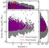 |
Fig. 1. Stellar mass to redshift distribution of the parent (grey points) and final (purple points) sample used in this paper for which reliable multi-wavelength size measurements can be performed (see text for details). The median stellar mass and redshift are shown as red lines. |
To avoid biases in our size–mass relations, we use the 80% mass completeness limits estimated in Weibel et al. (2024) per field and redshift bin. Without the mass limits our sample is biased to the bright and compact low-mass sources, resulting in a steeper size–mass relation.
Before proceeding with the derivation of the size–mass relation of galaxies, we have to ensure that the individual measurements are reliable. In particular, model fitting is naturally more reliable for sources with higher S/N. While the simultaneous fits across wavelength in principle allow us to relax the S/N requirements somewhat compared to a single-band fit, we still find that measurements become unreliable for sources with S/N < 10. We find that the bluest bands, that have lower S/N values, are fit with large and unrealistic effective radii (up to 40 kpc) if a S/N cut is not applied. Therefore, we require that all our sources are at least a 10σ detection in each of the six NIRCam filters (excluding F410M) that we use in the fits (see Section 3). The medium band is excluded as it may be biased to extreme line emission in these high-z star-forming galaxies e.g. O[III] + Hβ. With these S/N limits, our sample will not include any extremely red sources that disappear in shorter wavelength bands, such as HST-dark galaxies (Barrufet et al. 2023; Williams et al. 2024). For such sources with non-rest-UV detections, we cannot derive reliable rest-UV sizes.
One last class of sources we remove are so-called Little Red Dots (LRDs). These have originally been identified as broad-line emitters with point-like morphology in the reddest NIRCam filters (e.g. Matthee et al. 2024; Labbe et al. 2025). While some of these sources can still be dominated by star formation (e.g. Williams et al. 2024; Pérez-González et al. 2024), spectroscopy has revealed broad emission lines for the majority of these sources, consistent with an AGN component (e.g. Greene et al. 2024; Wang et al. 2024). Since we are only interested in estimating sizes for star-forming galaxies in this work, we remove these probable AGN. To do this, we apply the LRD colour selection from Labbe et al. (2025) (removing a total of 126 LRDs and compact red sources; Weibel et al. 2024) in addition to a size constraint as adopted in Gottumukkala et al. (2024) which removes a further 17 LRDs.
After applying the mass completeness, sSFR and S/N cuts as well as removing the LRDS, we have a parent sample of 3 ≤ z < 9 star-forming galaxies with size 4116.
2.6. Point spread functions (PSFs)
To measure accurate intrinsic sizes of galaxies, the use of reliable PSFs is crucial. In this work, we tested two different versions of PSFs, 1) created directly from stars in the images using ePSF from the Photutils package and 2) theoretical PSFs created using WebbPSF models (Perrin et al. 2014) that are drizzled in the same way as the science images. The first approach has the advantage that it is as close to the data as possible. However, in practice, it can be difficult to identify enough stars that are not saturated and contaminated by neighbouring sources. The wings of the PSFs can also be missed if the star cutouts are too small. This can also affect the PSF-matched fluxes and thus the physical parameters, e.g. stellar mass measured in SED fitting.
While the differences between the curves of growth are negligible between the two PSF models, the WebbPSF approach provides higher signal-to-noise models. We tested the two methods by fitting PSF models to stars in the CEERS field and found that the WebbPSF models performed slightly better than our empirical star models, resulting in smaller residuals on average. Therefore, we use the WebbPSF models in the following analysis.
3. Method
3.1. Wavelength dependent galaxy size measurements
To derive galaxy sizes, we fit single Sérsic models with a parametric model fitting tool called GalfitM (Häußler et al. 2013; Vika et al. 2013) to our selected z > 3 sample. GalfitM is an extension of the tool Galfit (Peng et al. 2010). The latter is a tool that fits the 2D surface brightness of a galaxy, after convolving a user-defined parametric model (e.g. Sérsic Model) with the PSF of the observation. GalfitM extends this work by fitting the 2D surface brightness of sources across multiple bands simultaneously. The wavelength dependence of the fitted parameters can be controlled using a polynomial, allowing for varying degrees of freedom between bands (set by a Chebyshev parameter).
GalfitM is run on stamps of 6 × 6 arcsec centred on each of our galaxies in the sample. Neighbouring sources are masked using a dilated version of the segmentation maps derived from SourceExtractor. This dilation is needed to remove external halo light from bright neighbours. We also derive a local background estimate for each source using a 3-σ clipped mean of all unmasked pixels. The background value is supplied to GalfitM and kept fixed while we fit for the Sérsic parameters for our central sources.
The initial guesses for individual Sérsic parameters are derived from the SourceExtractor catalogues. This includes the central coordinates (x, y), magnitude, axis ratio (b/a), and position angle (θ). The initial value of the effective radius and magnitude is taken to be the semi-major axis and the aperture corrected flux is measured by SourceExtractor. The effective radius is defined as the semi-major axis of the best-fit ellipse to the galaxy profile. The initial Sérsic index is set to 1.5, as our sample is expected to be star-forming galaxies and closer to disk-like structures. During the fits we set some constraints; the Sérsic values n are allowed to vary between 0.2 and 8, the effective radii to lie between 0.3 and 400 pixels (where 1 pixel = 0.04″), the axis ratios between 0.01 and 1 and magnitudes between 0 and 50.
We perform these Sérsic fits simultaneously over all NIRCam filters that are available in all our fields: F115W, F150W, F200W, F277W, F356W, F410M, and F444W. For these fits, we allow the magnitude and effective radii to vary independently across the different bands, in order not to bias our results. However, to minimise the number of free parameters, we fix the axis ratio, position angle, and coordinates, because we do not expect these values to change significantly with wavelength. The Sérsic index was allowed to vary quadratically with wavelength, as this reduced the number of unrealistic models, while not biasing the results.
Figure 2 shows four examples of input sources with their corresponding GalfitM model in their rest-UV and rest-optical bands. Residuals are also included to show the quality of the Sérsic fits.
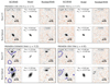 |
Fig. 2. Rest-UV and rest-optical fits of four star-forming galaxies in our sample (in 2″ images). In each block, the left column shows the signal-to-noise ratio images (science/sigma images) with contours showing the mask supplied to GalfitM (see Section 3). The middle column shows the best-fit PSF-convolved GalfitM Sérsic model to the source. The final box shows the signal-to-noise ratio of the residual image (residual/sigma images). |
3.2. GalfitM parameter uncertainties
GalfitM uncertainties are generally found to be underestimated3. This occurs because the software assumes that the model is a perfect fit to every unmasked pixel in the image. Therefore, the residual image should only contain Poisson noise (Häußler et al. 2013). However, this is unrealistic for real astronomical data.
To estimate realistic uncertainties, we thus follow a similar approach to van der Wel et al. (2012) and run a Monte-Carlo simulation on simulated images with known input model parameters, but using real blank field images. To do this, we identify 150 blank patches in the CEERS fields of the same size as our cutouts (6″ on a side). A Sérsic model, with parameters in the range of our real galaxy sample, is added to each of the 150 blank field cutouts. This is done for 250 Sérsic models which were randomly chosen from our sample. For each of these simulated cutouts, we further derived a corresponding RMS map that includes the Poisson noise of the model galaxy.
GalfitM was then run on each of the simulated images in the same way as our real data run (as discussed in Section 3). This includes starting from the same input parameters, constraints and using the same Chebyshev parameters as for the real galaxy fits. The only parameter that was changed was the background estimate, but the method for measuring this estimate is the same method used on the real data. For each simulated Sérsic model, we thus obtain 150 fits from the different blank field stamps. The standard deviation between these outputs provides us with an estimate of the real uncertainties in the different parameters, including the size, REFF. We find that the uncertainties derived from GalfitM are typically underestimated by factors up to ∼5×. We derive a correction factor through a linear relation between the log of the true standard deviation and the log of the REFF uncertainty derived by GalfitM. The best-fit parameters of these linear relations are presented in the Appendix (see Table A.1). Throughout the paper, we now use these empirically calibrated correction factors when quoting uncertainties on galaxy sizes.
3.3. Flags and source removal
Even after our initial S/N cuts, a small number of galaxies cannot be fit well with GalfitM. Following the practice in previous works, we thus removed sources for which the model fits to reach the limits of our constraints. We thus discarded sources with Sérsic index of > 7.8 or < 0.25, axis ratios of < 0.02 or > 0.95, and effective radii that were fit to be larger than the cutout size.
Finally, we visually inspected all the remaining fits and their residuals. Sources are removed if they have extremely bright and large neighbours within a few pixels of their segmentation map. Flux from such nearby neighbours is not completely removed by the applied masks, creating a bright background and affecting the fitting. We also check that individual fits do not have strong residuals following the residual flux fraction (RFF) method used in Ward et al. (2024) and Ormerod et al. (2024) but find that most of our fits lie below the 0.5 cut used in these works.
After removing all these sources from our parent sample, we are left with a final sample of 3529 star-forming galaxies. The breakdown by field and redshift bin can be seen in Table 1 and the distribution of redshift and stellar mass for both the parent and final sample are shown in Fig. 1.
Number of sources in the final section for each JWST field and for each redshift bin.
3.4. Measuring the size–mass relation
The galaxy size–mass relation has been shown to be well-approximated by a simple power law. Following past literature, we thus model the size–mass relation in the same way (e.g. van der Wel et al. 2014; Mowla et al. 2019; Ward et al. 2024). Specifically, we use the hierarchical Bayesian linear regression tool Linmix4 (Kelly 2007) to fit the mean relation as well as an intrinsic dispersion around the mean, σlogREFF. We fit a log-normal distribution to the size–mass relation as shown in Equation (2).
 (2)
(2)
Where REFF is the effective radius, α is the slope of the relation, M∗ is the stellar mass of a galaxy in solar masses, and logA is the intercept (i.e. the mean effective radius of galaxies of stellar mass 109 M⊙). Finally, σlogREFF is the intrinsic scatter, which measures the distribution in galaxy sizes at fixed stellar mass.
Linmix allows us to account for the uncertainties in both stellar mass and size measurements and it provides us with posterior samples for all the parameters from which we can derive the best-fit values as well as the uncertainties. We use Linmix to fit for α, logA and logσlogREFF for each NIRCam band in the three fields, in four redshift bins: 3 ≤ z < 4, 4 ≤ z < 5, 5 ≤ z < 6 and 6 ≤ z < 9. We exclude sources with REFF smaller than the PSF REFF at the sources’ photometric redshift. Due to low number statistics in the 6 ≤ z < 9 sample, we cannot constrain the size–mass relation without fixing the slope of the relation. Thus, based on our rest-optical parameter evolution measurements in Section 5.1 we have fixed the slope of our highest redshift bin to 0.215. Further work is needed to constrain the z > 6 size–mass relation and can be achieved by combining deep data sets, e.g. NGDEEP and JADES. The results of our fits are discussed in Section 4.
4. Results
Using the sizes derived in Section 3, we fit the size–mass relation (Equation (2)) for star-forming galaxies in four redshift bins: 3 ≤ z < 4, 4 ≤ z < 5, 5 ≤ z < 6 and 6 ≤ z < 9.
The extensive wavelength coverage of JWST/NIRCam in CEERS, PRIMER-UDS, and PRIMER-COSMOS, allows us to study galaxy sizes in seven bands: F115W, F150W, F200W, F277W, F356W, F410M and F444W. In the following, we first discuss the evolution of rest-frame optical size–mass relations, before we compare the size estimates at different wavelengths. For rest-UV measurements (2000 − 2500 Å) we use F115W, F150W, F200W and F277W, for each respective redshift bin. Similarly, for rest-optical measurements (4500 − 5500 Å), we use F200W, F277W, F356W and F444W.
When presenting the size–mass relation we include two shaded regions around the median fit. The darker region represents the 1σ uncertainty on the mean relation, while the lighter region shows the intrinsic scatter. For clarity, some plots in this paper omit the intrinsic scatter.
4.1. Rest-frame optical size evolution
Now with the high sensitivity and large near-infrared wavelength coverage of JWST, rest-optical galaxy size measurements can be extended to z ∼ 9 and down to stellar masses of ∼ 108 − 9 M⊙.
We present our rest-optical star-forming size–mass relations from z = 3 to z = 9 in Fig. 3 and Fig. 4. Due to low number statistics in the 6 ≤ z < 9 redshift bin (see right panel of Fig. 3), we fix fixed the size–mass slope to the average value measured over 3 ≤ z < 6 (see Section 3.4 and Section 4.1.3).
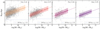 |
Fig. 3. Rest-optical size–mass relation across four redshift bins: 3 ≤ z < 4, 4 ≤ z < 5, 5 ≤ z < 6 and 6 ≤ z < 9. The solid black line represents the median fit, with its uncertainty in dark shading and intrinsic scatter in light grey. The grey open circles mark the data points used in the fit. The dotted line indicates the PSF size at the bin’s median redshift; points below this threshold REFF were excluded from fitting. In the highest redshift bin, due to limited data, we fixed the slope and fitted only the intercept and intrinsic dispersion (see Section 3.4). |
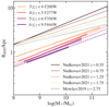 |
Fig. 4. Comparison of our z > 3 JWST-based rest-optical size–mass relations with z < 3 HST-based star-forming relations from Nedkova et al. (2021) and Mowla et al. (2019). The shaded regions indicate the 1σ fit uncertainties, while the intrinsic scatter is omitted for clarity. The slope of the 6 ≤ z < 9 relation is fixed (see Section 3.4). |
In Fig. 4, we find that the rest-optical size–mass relation evolves over the redshift range 3 ≤ z < 9, with galaxies becoming smaller and more compact at higher redshifts. However, it is easier to understand the evolution of the rest-optical, size–mass relation by studying the parameters and their evolution with redshift. Thus, we have parametrised the redshift evolution of the best-fit rest-optical size–mass parameters at different epochs between z = 3 and z = 9. The evolution of these parameters are presented in Fig. 5. We present the results of each parameter in Section 4.1.1, Section 4.1.2 and Section 4.1.3.
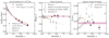 |
Fig. 5. Redshift evolution of the best-fit star-forming, rest-optical size–mass relation parameters. Left panel: Size evolution for galaxies at a fixed stellar mass of M* = 5 × 10¹⁰ M⊙ in the range 0.35 ≤ z < 9. Centre panel: Evolution of the slope, α. Right panel: evolution in the intrinsic scatter, σlogREFF. The diamonds and solid pink lines show the measurements and parametrised evolution from this paper. The HST-based measurements (Nedkova et al. 2021; Mowla et al. 2019; George et al. 2024; van der Wel et al. 2012) are shown in grey. The JWST-based studies from Ward et al. (2024) and Matharu et al. (2024) are shown in tan. The JWST-based work based on UV-bright ground-based selected star-forming galaxies from Varadaraj et al. (2024) are shown as grey squares. The HST-based parametrised fits to the redshift evolution from Mowla et al. (2019) and van der Wel et al. (2012) as well as the JWST-based size-evolution from Ward et al. (2024) are also included (see Table A.1 for values). |
In addition, we compare our rest-frame optical size–mass relations to low-z HST studies from Nedkova et al. (2021), Mowla et al. (2019) and van der Wel et al. (2014) as well as recent JWST-based studies from Ward et al. (2024), Matharu et al. (2024), Morishita et al. (2024) and Varadaraj et al. (2024). Each of these works measured the size–mass relation over different stellar mass ranges and there are systematics due to different methodologies, thus it is important to highlight these differences before comparing.
Nedkova et al. (2021), van der Wel et al. (2014), and Mowla et al. (2019) used HST data, applying UVJ colour selections to separate quiescent and star-forming galaxies. Nedkova et al. (2021) measured rest-5000 Å sizes of 0 < z < 2 star-forming galaxies at stellar masses of 8 < log(M*/M⊙) < 11.5, while van der Wel et al. (2014) covered 0 < z < 3 galaxies at stellar masses of 9 < log(M*/M⊙) < 11.5. Mowla et al. (2019) extended this work to include log(M*/M⊙) > 11.3 galaxies. Both van der Wel et al. (2014) and Mowla et al. (2019) used single S’ersic models in the H160 band with Galfit. Nedkova et al. (2021) used GalfitM and the Chebyshev polynomials to calculate then rest-5000 Å sizes. With the recent JWST data, Ward et al. (2024) studied log(M*/M⊙) > 9.5 galaxies (over the redshift range of 0.5 < z < 5.5) selected with SED fitting from the CEERS dataset. This work is similar to our approach in this paper. Matharu et al. (2024) differs in that their measurements are made on stacks of hundreds of (8 < log(M*/M⊙) < 10) galaxies in the F444W band from FRESCO, while Varadaraj et al. (2024) focused on bright 3 ≤ z < 5 LBGs (in the stellar mass range of 9 < log(M*/M⊙) < 11) from the PRIMER survey, initially selected by ground-based data. Finally, Morishita et al. (2024) and Ono et al. (2024) measured sizes of 4 < z < 14 galaxies, with Morishita et al. (2024) using a combined dataset from nine JWST surveys with spectroscopic confirmed sources and Ono et al. (2024) selecting galaxies from CEERS.
4.1.1. Redshift evolution of star-forming galaxies of stellar mass 5 × 10¹⁰ M⊙ rest-optical sizes
The effective radius measurements for galaxies of stellar mass M∗ = 5 × 10¹⁰ M⊙ are plotted in the left panel of Fig. 5. This stellar mass is chosen such that we can fairly compare our measurements with previous estimates from the literature. We note, however, that our samples of galaxies at those high masses are small and the values we show mostly rely on the size–mass relation fits to lower mass galaxies.
From the plot, it is evident that the size evolution in star-forming galaxies at this fixed mass is well fit by a log-linear relation over the period of 0 < z < 9:
 (3)
(3)
We thus combine our rest-optical size estimates at z > 3 with values measured at z < 3 from van der Wel et al. (2014), to fit for the parameters in Equation (3) over the total redshift range of 0 < z < 9. Over this period, we find that the size-evolution of star-forming galaxies of mass M* = 5 × 10¹⁰ M⊙ follows the function logREFF = ( − 0.807 ± 0.026)×log10(1 + z)+(0.947 ± 0.014). This is shown in the left panel of Fig. 5 as a solid line and indicates that a typical star-forming galaxy of M∗ = 5 × 10¹⁰ M⊙ grows rapidly by a factor of 2× from z ∼ 8 to z ∼ 3 and then another factor of 3× to z ∼ 0.
Interestingly, our measured evolution is in relatively good agreement with extrapolations from lower redshifts from van der Wel et al. (2014) and Mowla et al. (2019), as well as with recent JWST-based estimates from Ward et al. (2024). Our measured average sizes at z ∼ 4 − 6, are within 1σ of the parametrised evolution predicted by HST-based, z < 3 studies.
4.1.2. Evolution of the distribution in rest-optical sizes of star-forming galaxies at 3 ≤ z < 9
To study the distribution of galaxy sizes over time, we have plotted our measured intrinsic dispersion values in the range 3 ≤ z < 9 in the right panel of Fig. 5. While the measured values vary somewhat, we find that the intrinsic dispersions are consistent with a constant value of σlogREFF = 0.188 ± 0.007, over the redshift range z = 3 to z = 9. This is within a 1σ agreement with the rest-optical intrinsic scatter measured by van der Wel et al. (2014) at lower redshifts. Our rest-optical intrinsic scatter data points at z = 3.5, z = 4.5 and z = 5.5, are within 1 − 2σ of the z = 4.2 rest-optical and z = 5.7 stacked F444W intrinsic scatter measurements by Ward et al. (2024) and Matharu et al. (2024), respectively. However, we find > 2σ differences with the intrinsic scatter measured by Morishita et al. (2024) and Varadaraj et al. (2024), who find larger values for galaxies in the range 4 < z < 14 and 3 < z < 6, respectively. This difference could be due to both studies fitting the size–mass relation for Lyman break galaxies (LBGs). Also, as discussed in Section 4.3, the size of a galaxy varies depending on the wavelength it was measured in. This could also lead to the difference between our work and Varadaraj et al. (2024), who only measures galaxy sizes in F200W and F356W.
Except for these two estimates, the intrinsic dispersion measurements of all literature results lie in the range σlogREFF = 0.15 − 0.25 dex. Overall, these results thus indicate, at fixed stellar mass, that the dispersion of star-forming galaxy sizes around the mean stays rather constant across the full redshift range probed to date.
4.1.3. Evolution of the rest-optical size–mass slope
Finally, we discuss the slope measurements of the rest-optical size–mass relation, which are plotted in the central panel of Fig. 5. In our sample of star-forming galaxies at z = 3 − 9, we find slopes that are consistent with each other within 1 − 2σ at all redshift. The average value is found to be α = 0.215 ± 0.009 over the redshift range of 3 ≤ z < 9. This value is consistent within 1σ with van der Wel et al. (2014) who found that the average size–mass slope is α = 0.22, for star-forming galaxies in the range 0 < z < 3. Similar values are also found by Ward et al. (2024) and Matharu et al. (2024) at z ∼ 4 − 5, and even by Morishita et al. (2024) who analysed galaxies out to z ∼ 14. This could indicate that the steepness of the size–mass relation of star-forming galaxies remains unchanged over the full cosmic history at a value of α = dlogREFF/dlogM* ∼ 0.2.
This result is different from previous extrapolations of lower-redshift trends from Mowla et al. (2019), for example, who found a trend to flatter slopes to higher redshifts (see central of panel Fig. 5), in line with the estimates from Varadaraj et al. (2024) at z = 3 − 5. It will thus be important to revisit the size–mass relation estimates in the future with larger samples also extending to lower and higher masses to test whether the slopes stay constant over redshift, or if they might evolve.
4.2. The rest-optical and rest-UV size–mass relations star-forming galaxies
To understand the build-up of stellar mass in z > 3 star-forming galaxies, we investigate galaxy size measurements in rest-UV and rest-optical. The rest-UV and rest-optical size–mass relations in three redshift bins are presented in Fig. 6. The highest redshift bin is not shown due to the small number of galaxies that prevents us from accurately fitting for the slope of the size–mass relations (see Fig. 3).
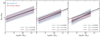 |
Fig. 6. Star-forming size–mass relations in rest-UV (blue) and rest-optical (red) across three redshift bins: 3 ≤ z < 4, 4 ≤ z < 5, and 5 ≤ z < 6 (left to right). The median fit is shown with two shaded regions: the 1σ fit uncertainty and the median intrinsic scatter. The 3 ≤ z < 4 relation is plotted as a black dashed line in all panels. At z < 5, rest-UV and rest-optical relations are within 1σ but at z > 5, star-forming galaxies with log(M*/M⊙) < 9 are > 2σ smaller in rest-UV. |
In all three panels we can see that over the stellar mass range of 8 < log(M*/M⊙) < 11, the rest-optical and rest-UV relations are within 1σ of each other, except in the z ∼ 5 − 6 bin, where the rest-UV size–mass relation appears to be steeper than the rest-optical one. The mean size of 5 ≤ z < 6 star-forming galaxies with stellar mass log(M*/M⊙) ≤ 9, are > 2σ smaller in rest-UV than in rest-optical wavelengths. More details are discussed in Section 5.2.
Interestingly, at all redshifts, we find the intrinsic dispersion of the size–mass relation to be larger in the rest-UV compared to the rest-frame optical, hinting at a wavelength dependence. We investigate these trends further in the next section.
4.3. The wavelength dependence of the size–mass relation parameters
Due to the extended NIRCam wavelength coverage, we can investigate the size–mass relation over multiple wavelengths spanning rest-UV and rest-optical, including longer wavelengths than rest-frame 0.5 μm, (in the three lower redshift bins). This is important to understand the stellar mass build-up of galaxies. Fig. 7 shows the variation in the size–mass relation parameters that we fit for as a function of rest-frame wavelength. The rest-frame wavelength for each NIRCam band is calculated using the median redshift of a given bin. These parameters and median redshifts are specified in Table A.1.
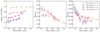 |
Fig. 7. Best-fit parameters of the star-forming size–mass relation: intercept in kpc at 109 M⊙ (left), slope α (centre), and intrinsic scatter σlogREFF (right) as functions of rest-frame wavelength (using median redshifts per bin; see Table A.1). The 6 ≤ z < 9 slope is omitted from the centre panel as it was fixed during fitting (see Section 3.4). The observed decrease in slope with wavelength aligns with colour gradients, while the large σlogREFF at λ < 0.5 μm may reflect off-centre bursty star formation in z > 3 star-forming galaxies. |
The left panel of Fig. 7 shows the sizes of log(M*/M⊙) = 9 star-forming galaxies in four redshift bins. In all redshift ranges, the sizes of star-forming galaxies are consistent within 1σ in the wavelength range of 0.15 μm < λ < 0.5 μm. This behaviour also continues to 1 μm for 3 ≤ z < 5 star-forming galaxies. However, there is an indication that the sizes of log(M*/M⊙) = 9 star-forming galaxies, at z > 5, positively increase at λ > 0.5 μm, although this trend is uncertain due to the large errors.
This figure also shows that for a given rest-frame wavelength, the average size of log(M*/M⊙) = 9 star-forming galaxies decreases to higher redshift. The rate of this decrease is somewhat wavelength-dependent, with rest-UV sizes decreasing slightly faster than rest-optical sizes.
To further examine the dependence of galaxy size with stellar mass, we show the slope of the size–mass relation as a function of rest-frame wavelength in the central panel of Fig. 7, except for the highest redshift bin (for which the slope cannot be measured accurately). For all three redshift bins in the range 0.2 μm < λ < 0.8 μm, there is a general indication of a decreasing trend with increasing wavelength i.e. the longer wavelength size–mass relations become flatter). However, given the errors, this downward trend is uncertain.
Focusing on the slopes from the 3 ≤ z < 4 size–mass relation that we can determine best, we see roughly a constant slope of α = 0.2 at wavelengths of λ < 0.5 μm, which then starts to flatten to α = 0.1 at λ = 1 μm. This trend is also observed in the 4 ≤ z < 5 redshift bin, but is uncertain due to the large errors. We discuss the implications of this on galaxy stellar mass build-up further in Section 5.3.
Finally, the right panel in Fig. 7 shows the intrinsic scatter as a function of rest-frame wavelength. For all redshift bins the intrinsic scatter starts high around a value of ∼0.22 − 0.25 dex in rest-UV and then falls and plateaus to values in the range ∼0.17 − 0.19 dex, at wavelengths λ > 0.5 μm. This shows that the dispersion in galaxy sizes at a fixed mass becomes 10% smaller when measured in redder wavelengths compared to rest-UV and this trend is independent of redshifts in the range 3 ≤ z < 9, within current uncertainties.
Overall, our analysis thus reveals that the size–mass relation of star-forming galaxies at z ∼ 3 − 8 has a higher dispersion and steeper slope in the rest-frame UV compared to longer rest-frame wavelengths. The implications of this are discussed in section 5.2.
5. Discussion
In this section, we discuss the two main results presented in this paper: the redshift evolution of the rest frame optical sizes (Section 5.1), and the wavelength dependence of the size–mass relation parameters (Section 5.2). We also comment on comparisons with simulations that have measured the size mass relation at z > 3 (Section 5.4) and compare to low-z rest-NIR studies (Section 5.3).
5.1. Analysis of the rest-frame optical size evolution
In Section 4.1 we found that the rest-optical size–mass slope and intrinsic dispersion are consistent with each other over 3 ≤ z < 9 and their evolution can be well described by a constant. This provides some interesting clues on the relation between the galaxies and their dark matter halos.
Simple galaxy disk models predict a correlation between the dispersion in dark matter halo spin and the amount of scatter in the size–mass relation (see e.g. Mo et al. 1998, Ward et al. 2024, van der Wel et al. 2014, and citations within). Most simulations have measured the dispersion of the DM spin parameter to be 0.2 − 0.25 dex (log base 10) (e.g. Macciò et al. 2008; Burkert et al. 2016). This is consistent with our average intrinsic scatter of σlogREFF = 0.188 ± 0.007, over the redshift range of 3 ≤ z < 9. This provides further support that the sizes of star-forming galaxies at z > 3 are indeed driven by their dark matter halo spins, even in the early Universe.
Additionally, the slope of the size–mass relation carries information on the ratio of stellar to halo masses. As described in the introduction, we expect a slope of αDM = 1/3  for DM halos. This is steeper than the constant slope of the size–galaxy mass relationship we found (α = 0.215 ± 0.009) at z = 3 − 9. Such a difference in slopes can be explained if the relation between the stellar mass and halo mass is not a constant, which has also been found in previous works (e.g., van der Wel et al. 2014, Ward et al. 2024 and Shen et al. 2003).
5.2. Sizes of star-forming galaxies in multi-wavelength observations
In this section, we discuss the results of the wavelength dependence on the size–mass relation and its parameters.
As shown in the right panel of Fig. 7, the intrinsic scatter decreases with increasing wavelength for all redshift bins and over the stellar mass range for which we measure the size–mass relations. A higher intrinsic scatter in rest-UV compared to rest-optical has also been measured for z = 5 bright LBGs in Varadaraj et al. (2024) as well as for star-forming galaxies at z < 1 in George et al. (2024). High levels of intrinsic scatter indicate significant variations in measured sizes. Bursts of star formation are often short-lived, compact and not necessarily spatially coherent from galaxy-to-galaxy (see e.g. Giménez-Arteaga et al. 2024). Recent studies further suggest that star formation at z > 4 is bursty (Looser et al. 2024; Carnall et al. 2023; Curti et al. 2024). Since rest-UV wavelengths trace star formation on short timescales (∼100 Myr) significant variations in the rest-UV sizes (plus smaller variations in rest-optical sizes) are likely a result of bursty star formation.
The left and centre panels of Fig. 7 show no significant wavelength dependence on the intercept or slope over the range 0.15 μm < λ < 0.6 μm. This is further illustrated in Fig. 6 for the full mass range we fit over. These results suggest that, on average rest-UV and rest-optical sizes are similar for star-forming galaxies from z = 3 to z = 9. JWST-based studies from Morishita et al. (2024) and Ono et al. (2024) found that the ratio between rest-UV and rest-optical sizes are ∼1. Likewise, Ormerod et al. (2024) reports that 3 < z < 8 star-forming galaxies at log(M*/M⊙) < 9.5 are consistent within 1σ across the observed wavelength range of 1 μm < λobs < 5 μm. These similar sizes at low stellar masses suggest several possibilities: (1) these galaxies are young and haven’t built up their older stellar population (Morishita et al. 2024; Ono et al. 2024), (2) outshining effects from highly star-forming clumps dominate their light profiles (Giménez-Arteaga et al. 2024), or (3) compact dust attenuation biases the measured sizes in these wavelengths.
At wavelengths λ > 0.5 μm, there is a general decrease in the slope of the size–mass relation (centre panels of Fig. 7). This flattening of the slope is seen up to 1 μm for our 3 ≤ z < 4 redshift bin. Smaller rest-1 μm sizes in comparison to rest-UV and rest-optical sizes suggest colour gradients could play a role in flattening the slope. We discuss this further in Section 5.3.
5.3. The decreasing slope behaviour of 3 < z < 4 star-forming galaxy size–mass relation
In this section, we investigate the behaviour of the decreasing size–mass slope with increasing wavelength, for star-forming galaxies at 3 ≤ z < 4. With the large NIR coverage of JWST NIRCam, the sizes of 3 ≤ z < 4 galaxies can be measured at wavelengths up to ∼1 μm. NIR wavelengths are less affected by dust and thus are expected to most accurately trace the underlying mass distribution of the stellar population. By fitting a linear relation to the ratio of the rest-optical and rest-1 μm sizes (presented in Fig. 8) we find that log(M*/M⊙) > 10 star-forming galaxies at 3 < z < 4 are smaller by ∼10% in rest-1 μm than 0.5 μm. In contrast for log(M*/M⊙) < 10 star-forming galaxies, no significant difference in size is observed between these two wavelengths, suggesting that more massive galaxies are contributing to the flattening of the size–mass slope. Previous works from Suess et al. (2022) and Martorano et al. (2024), presented in Fig. 8, have also found similar trends in size differences between the rest-NIR and rest-optical wavelengths and are in good agreement without work.
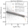 |
Fig. 8. Ratio of size–mass relations in F444W and F200W at 3 ≤ z < 4: the black line represents rest-frame ∼1 μm and ∼0.5 μm with dashed segments extrapolating to log(M*/M⊙) > 11. JWST-based results from Suess et al. (2022) and Martorano et al. (2024) are shown as coloured solid lines and squared points. Star-forming galaxies at log(M*/M⊙) > 9.5 are ≳10% smaller in rest-1 μm than in rest-0.5 μm consistent of colour-gradients (see Section 5.3) and lower-z studies. |
Smaller rest-1 μm sizes in comparison to rest-optical suggest colour gradients in 3 ≤ z < 4 star-forming galaxies of log(M*/M⊙) > 10. These colour gradients can indicate inside-out-growth, build-up of bulges, or the effects of dust attenuation. Recent JWST studies have also found indications of colour gradients in z < 3 star-forming galaxies (Suess et al. 2022, Martorano et al. 2024, van der Wel et al. 2024). These colour gradients could be a result of compact dust attenuation in the centre of these high-mass star-forming galaxies. Larger dust fractions in more massive galaxies have also been found by other studies (e.g. Whitaker et al. 2017; Fudamoto et al. 2020; Magnelli et al. 2024; Weibel et al. 2024) and the spatial distribution of this dust in z > 2.5 star-forming galaxies has been found to be located centrally in some simulations (e.g. Wu et al. 2020, Marshall et al. 2022, Roper et al. 2022, Popping et al. 2022) and observational studies (Tacchella et al. 2018; Wang et al. 2017; Nelson et al. 2016; Gómez-Guijarro et al. 2022; Fujimoto et al. 2017). Although, the dust distribution in high-z galaxies is still uncertain partly due to limitations of current facilities (e.g. ALMA and NOEMA) that require long integration times for higher resolution data and for detecting the low surface brightness from the outskirts. Further work on obtaining large samples of high-resolution dust detection of star-forming galaxies in addition to resolved stellar population fitting is needed to understand the effects of dust on galaxy morphology.
5.4. Comparisons to simulations
In this section, we discuss the findings of some simulations on the wavelength dependence on galaxy sizes and also compare the observed 5 ≤ z < 6 size–mass relation with predictions.
In Section 4 we find that the parameters of the size–mass relation have a wavelength dependence, such as the intrinsic scatter which is larger in rest-UV wavelengths than in wavelengths at λ ≥ 0.5 μm for all our redshift bins. These findings align with results from the FIRE simulation for star-forming galaxies (7.5 < log(M*/M⊙) < 8) z ≥ 5. The FIRE model finds less scatter between half-stellar mass radii and rest B-band sizes compared to the scatter between half-stellar mass radii and rest-UV sizes. Ma et al. (2018) shows that the rest-UV sizes trace the small, bright young stellar clumps within these high-z galaxies, and these clumps do not represent the total stellar mass.
Analysis of the size–mass relation for star-forming galaxies at 3 ≤ z < 6 shows a systematic trend in which the slope decreases progressively from rest-UV to rest-optical and continues up to rest-1 μm wavelengths for the redshift bins where longer wavelength data are available. This wavelength dependence is consistent with numerical simulations of star-forming galaxies at 5 < z < 10 with stellar masses 9 < log(M*/M⊙) < 11.5 (Roper et al. 2023; Marshall et al. 2022). These simulations find that the bulk of the stellar distribution of log(M*/M⊙) > 9.5 star-forming galaxies at z > 5 is compact and attenuated by centrally compact dust profiles. This dust attenuates/dims the star-forming core so that star formation in the outskirts of these galaxies can be measured. Consequently, wavelengths bluer than NIR may systematically overestimate intrinsic galaxy sizes (Roper et al. 2023; Marshall et al. 2022; Popping et al. 2022). However, the negative slopes predicted by these simulations in NIR wavelengths disagree with our observed relations. Further work probing rest-NIR wavelengths at z > 3 is essential to investigate the flattening of the size–mass relation. The JWST/MIRI instrument can provide rest-NIR observations of galaxies at z > 3, but with reduced spatial resolution compared to the NIRCam wavelength range.
We compare our 5 ≤ z < 6 size–mass relation with predictions from three simulations; IllustrisTNG (Costantin et al. 2023), THESAN (Shen et al. 2024a) and ASTRID (LaChance et al. 2024), each of which provides size–mass relations for galaxies at z = 5 and z = 6. The analysis of IllustrisTNG by Costantin et al. (2023) utilizes the TNG-50-1 simulation, the highest resolution configuration within the IllustrisTNG framework, focusing on star-forming galaxies with stellar masses 9.5 < log(M*/M⊙) < 12 across the redshift range 3 < z < 7. A comparable mass selection is employed by LaChance et al. (2024) in their analysis of the ASTRID simulation for galaxies at 3 < z < 6. Both studies create mock NIRCam observations that represent CEERS survey specifications and derive galaxy sizes through parametric fitting with the python-based software, statmorph. The work from Shen et al. (2024a) analyses galaxy sizes at 6 < z < 10 using noiseless mock observations derived from the THESAN project: a suite of large-volume cosmological radiation-magneto-hydrodynamic simulations of the Epoch of Reionisation. Apparent sizes in UV- and V-band 2D are computed as brightness-weighted median radial distances from galactic centres.
The predicted z > 5 size–mass relations from these models are included in Fig. 9 with our 5 ≤ z < 6 observed relation. Over the stellar mass range 9 ≤ log(M*/M⊙) < 10, there is good agreement with the observed and predicted relations, given the scatter. However, at log(M*/M⊙) > 10, the observed relation has a steeper (positive) slope compared to the predictions from all three models. Although ASTRID predicts a positive slope at these high masses, it is offset by 0.5 dex from the observed relation. IllustrisTNG and THESAN find smaller sizes for high-mass galaxies in their models, which disagrees with the observed positive relation.
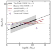 |
Fig. 9. Comparison of our 5 ≤ z < 6 F356W star-forming size–mass relation with three simulations: THESAN (Shen et al. 2024a), IllustrisTNG (Costantin et al. 2023) and ASTRID (LaChance et al. 2024). The observations and simulations align between 9 ≤ log(M*/M⊙) < 10 but diverge at log(M*/M⊙) > 10, due to the compact high-mass galaxies in simulations. |
Theoretical models are consistently finding negative slopes from the intrinsic size–mass and size–luminosity relations, caused by highly compact massive galaxies (e.g. Roper et al. 2022; Marshall et al. 2022; Shen et al. 2024a; Popping et al. 2022). The physical mechanisms leading to these compact sizes are still being studied. Two possible pathways seen in simulations are: either stars form in dense, pristine gas at z > 10 and maintain their compact configuration until z = 4, or initially diffuse galaxies undergo concentrated central star formation below z = 10, becoming compact by z ∼ 5 (see e.g. Roper et al. 2023; Marshall et al. 2022). Observational evidence for the run-away star formation mechanisms found in simulations is required. As discussed in Section 5.3 our measurements may still be affected by dust and colour gradients. The latter requires further work using Integral Field Unit (IFU) data, dust mapping or spatially resolved SED fitting (e.g. Giménez-Arteaga et al. 2023). Furthermore, our high-z sample is still limited to log(M*/M⊙) < 10.4 star-forming galaxies. Large and deep surveys such as COMSOS-Web (Casey et al. 2023) are needed to probe these high-mass sources and constrain the high-mass end of the size–mass relation in more detail.
6. Conclusion
For this paper, we studied the size–mass relation for star-forming galaxies in the range 3 ≤ z < 9. By combining three fields: CEERS, PRIMER-UDS and PRIMER-COSMOS, we were able to fit the size–mass relation over the mass range of 8 ≲ log(M*/M⊙) ≲ 10.5 and over six NIRCam bands. We selected z ≥ 3 star-forming galaxies using the SED fitting software Eazy, and measured stellar masses and other physical parameters with Bagpipes. With the multi-wavelength model fitting tool GalfitM, we measured the sizes of 3529 star-forming galaxies by fitting single Sérsic profiles over six NIRCam wide-filter bands. We used this to estimate the wavelength-dependent size–mass relation in four redshift bins: 3 ≤ z < 4, 4 ≤ z < 5, 5 ≤ z < 6, and 6 ≤ z < 9 using the Bayesian linear regression tool Linmix. The main results are as follows.
-
We find that the redshift evolution in the average sizes of M∗ = 5 × 10¹⁰ M⊙ star-forming galaxies is well fit by a power-law function of logREFF = ( − 0.807 ± 0.026)×log10(1 + z)+(−0.947 ± 0.014), over 3 ≤ z < 9. This indicates that a typical star-forming galaxy of this mass grows rapidly by a factor of 2× from z ∼ 8 to z ∼ 3 and then another factor of 3× to z ∼ 0.
-
Through studying the evolution of the rest-optical size–mass parameters, we find that the evolution of the slope and intrinsic scatter are well fit by a constant over 3 ≤ z < 9, where these values are α = 0.215 ± 0.009 and σlogREFF = 0.188 ± 0.007. The processes that flatten the star-forming size–mass slope, compared to the relation of stellar-to-halo size, acts similarly across all redshifts.
-
With the large NIRCam wavelength coverage in all three fields, we were able to parametrise the size–mass relation as a function of wavelength and redshift. We find that the slope and intrinsic scatter have a wavelength dependence, while the intercept shows no significant dependence. These parameters are largest in rest-UV in comparison to redder wavelengths. We speculate that bursty star formation, traced by rest-UV wavelengths, causes these wavelength dependences.
-
We find evidence of colour gradients in 3 ≤ z < 4 star-forming galaxies with log(M*/M⊙) > 9.5. These sources are smaller in rest-1 μm in comparison to rest-optical (and rest-UV) wavelengths. Possible suggestions for these colour gradients are inside-out growth or bulge growth in massive galaxies at this epoch, as well as compact and central dust profiles – suggested by simulations – which attenuate the central star-forming core so that star formation in the outskirts is measured.
-
Finally, we compared our 5 ≤ z < 6 star-forming size–mass relation to three simulations. We find a general good agreement between the observed and simulated size–mass relations over 9 ≤ log(M*/M⊙) < 10. However, beyond this mass, the observed relation is significantly steeper than any of the simulated relations – which are flattened due to extremely compact galaxies at high masses. Such galaxies are not seen in our current sample.
Future work on combining larger and deeper surveys such as COSMOS-Web is needed to constrain the size evolution of the most massive galaxies. Incorporating deeper surveys such as JADES and NGDEEP will enable robust measurements of the size–mass slope at z > 6, determining whether or not the steepening of the size–mass relation continues towards higher redshifts. Further work in understanding the mechanism driving highly compact massive galaxies in simulations is also needed. Finally, larger surveys with MIRI imaging are required to measure rest-NIR and rest-optical sizes at higher-z to enable the study of colour gradients and how they affect our understanding of galaxy growth. IFU or spatially resolved SED fitting can also shed light on the cause of these colour gradients. This study highlights the importance of measuring sizes at multiple wavelengths in order to reduce biases and understand galaxy growth.
The DAWN JWST Archive (DJA) is a repository of public JWST data, reduced with grizli and msaexp, and released for use by anyone: https://dawn-cph.github.io/dja/index.html
This has been discussed by the author of Galfit here: https://users.obs.carnegiescience.edu/peng/work/galfit/TFAQ.html#errors under the topic ‘Why are the error bars/uncertainties quoted in “fit.log” often so small?’.
Acknowledgments
The authors thank the referee for a helpful report that has improved the paper. The authors acknowledge the CEERS and PRIMER teams for developing their observing programme with a zero-exclusive-access period. This work is based on observations made with the NASA/ESA/CSA James Webb Space Telescope. The raw data were obtained from the Mikulski Archive for Space Telescopes at the Space Telescope Science Institute, which is operated by the Association of Universities for Research in Astronomy, Inc., under NASA contract NAS 5-03127 for JWST. This research is also based on observations made with the NASA/ESA Hubble Space Telescope obtained from the Space Telescope Science Institute, which is operated by the Association of Universities for Research in Astronomy, Inc., under NASA contract NAS 5–26555. The data products presented herein were retrieved from the Dawn JWST Archive (DJA). DJA is an initiative of the Cosmic Dawn Center, which is funded by the Danish National Research Foundation under grant DNRF140. This work has received further funding from the Swiss State Secretariat for Education, Research and Innovation (SERI) under contract number MB22.00072, as well as from the Swiss National Science Foundation (SNSF) through project grant 200020_207349. R.G.V. acknowledges funding from the Science and Technology Facilities Council (STFC; grant code ST/W507726/1). F.V. acknowledges support from the Independent Research Fund Denmark (DFF) under grant 3120-00043B. Software: Astropy, Eazy (Brammer et al. 2008), Galfit, GalfitM (Häußler et al. 2013; Vika et al. 2013), Grizli (Brammer 2023), WebbPSF (Perrin et al. 2014), Bagpipes (Carnall et al. 2018)
References
- Bagley, M. B., Finkelstein, S. L., Koekemoer, A. M., et al. 2023, ApJ, 946, L12 [NASA ADS] [CrossRef] [Google Scholar]
- Barrufet, L., Oesch, P. A., Weibel, A., et al. 2023, MNRAS, 522, 449 [NASA ADS] [CrossRef] [Google Scholar]
- Bertin, E., & Arnouts, S. 1996, A&AS, 117, 393 [NASA ADS] [CrossRef] [EDP Sciences] [Google Scholar]
- Bouwens, R. J., Illingworth, G. D., van Dokkum, P. G., et al. 2022, ApJ, 927, 81 [NASA ADS] [CrossRef] [Google Scholar]
- Brammer, G. 2023, https://zenodo.org/records/8370018 [Google Scholar]
- Brammer, G. B., Van Dokkum, P. G., & Coppi, P. 2008, ApJ, 686, 1503 [Google Scholar]
- Burkert, A., Förster Schreiber, N. M., Genzel, R., et al. 2016, ApJ, 826, 214 [Google Scholar]
- Calzetti, D., Armus, L., Bohlin, R. C., et al. 2000, ApJ, 533, 682 [NASA ADS] [CrossRef] [Google Scholar]
- Carnall, A. C., McLure, R. J., Dunlop, J. S., & Davé, R. 2018, MNRAS, 480, 4379 [Google Scholar]
- Carnall, A. C., Walker, S., McLure, R. J., et al. 2020, MNRAS, 496, 695 [Google Scholar]
- Carnall, A. C., Begley, R., McLeod, D. J., et al. 2023, MNRAS, 518, L45 [Google Scholar]
- Casey, C. M., Kartaltepe, J. S., Drakos, N. E., et al. 2023, ApJ, 954, 31 [NASA ADS] [CrossRef] [Google Scholar]
- Chabrier, G. 2003, PASP, 115, 763 [Google Scholar]
- Costantin, L., Pérez-González, P. G., Vega-Ferrero, J., et al. 2023, ApJ, 946, 71 [NASA ADS] [CrossRef] [Google Scholar]
- Curti, M., Maiolino, R., Curtis-Lake, E., et al. 2024, A&A, 684, A75 [NASA ADS] [CrossRef] [EDP Sciences] [Google Scholar]
- Curtis-Lake, E., McLure, R. J., Dunlop, J. S., et al. 2016, MNRAS, 457, 440 [NASA ADS] [CrossRef] [Google Scholar]
- Cutler, S. E., Whitaker, K. E., Mowla, L. A., et al. 2022, ApJ, 925, 34 [NASA ADS] [CrossRef] [Google Scholar]
- Dunlop, J. S., Abraham, R. G., Ashby, M. L. N., et al. 2021, PRIMER: Public Release IMaging for Extragalactic Research, JWST Proposal. Cycle 1, ID. #1837 [Google Scholar]
- Eldridge, J. J., Stanway, E. R., Xiao, L., et al. 2017, PASA, 34, e058 [Google Scholar]
- Fall, S. M., & Efstathiou, G. 1980, MNRAS, 193, 189 [NASA ADS] [CrossRef] [Google Scholar]
- Finkelstein, S. L., Bagley, M. B., Arrabal Haro, P., et al. 2022, ApJ, 940, L55 [NASA ADS] [CrossRef] [Google Scholar]
- Fudamoto, Y., Oesch, P. A., Faisst, A., et al. 2020, A&A, 643, A4 [NASA ADS] [CrossRef] [EDP Sciences] [Google Scholar]
- Fujimoto, S., Ouchi, M., Shibuya, T., & Nagai, H. 2017, ApJ, 850, 83 [Google Scholar]
- George, A., Damjanov, I., Sawicki, M., et al. 2024, MNRAS, 528, 4797 [NASA ADS] [CrossRef] [Google Scholar]
- Giménez-Arteaga, C., Oesch, P. A., Brammer, G. B., et al. 2023, ApJ, 948, 126 [CrossRef] [Google Scholar]
- Giménez-Arteaga, C., Fujimoto, S., Valentino, F., et al. 2024, A&A, 686, A63 [NASA ADS] [CrossRef] [EDP Sciences] [Google Scholar]
- Gómez-Guijarro, C., Elbaz, D., Xiao, M., et al. 2022, A&A, 658, A43 [NASA ADS] [CrossRef] [EDP Sciences] [Google Scholar]
- Gottumukkala, R., Barrufet, L., Oesch, P. A., et al. 2024, MNRAS, 530, 966 [NASA ADS] [CrossRef] [Google Scholar]
- Greene, J. E., Labbe, I., Goulding, A. D., et al. 2024, ApJ, 964, 39 [CrossRef] [Google Scholar]
- Grogin, N. A., Kocevski, D. D., Faber, S. M., et al. 2011, ApJS, 197, 35 [NASA ADS] [CrossRef] [Google Scholar]
- Häußler, B., Bamford, S. P., Vika, M., et al. 2013, MNRAS, 430, 330 [Google Scholar]
- Hopkins, P. F., Hernquist, L., Cox, T. J., Keres, D., & Wuyts, S. 2009, ApJ, 691, 1424 [Google Scholar]
- Huang, K.-H., Fall, S. M., Ferguson, H. C., et al. 2017, ApJ, 838, 6 [NASA ADS] [CrossRef] [Google Scholar]
- Ito, K., Valentino, F., Brammer, G., et al. 2024, ApJ, 964, 192 [CrossRef] [Google Scholar]
- Kamieneski, P. S., Frye, B. L., Pascale, M., et al. 2023, ApJ, 955, 91 [NASA ADS] [CrossRef] [Google Scholar]
- Kawamata, R., Ishigaki, M., Shimasaku, K., et al. 2018, ApJ, 855, 4 [NASA ADS] [CrossRef] [Google Scholar]
- Kelly, B. C. 2007, ApJ, 665, 1489 [Google Scholar]
- Koekemoer, A. M., Faber, S. M., Ferguson, H. C., et al. 2011, ApJS, 197, 36 [NASA ADS] [CrossRef] [Google Scholar]
- Kroupa, P., Tout, C. A., & Gilmore, G. 1993, MNRAS, 262, 545 [NASA ADS] [CrossRef] [Google Scholar]
- Labbe, I., Greene, J. E., Bezanson, R., et al. 2025, ApJ, 978, 92 [NASA ADS] [CrossRef] [Google Scholar]
- LaChance, P., Croft, R., Ni, Y., et al. 2024, Open J. Astrophys., 8, 20 [Google Scholar]
- Looser, T. J., D’Eugenio, F., Maiolino, R., et al. 2024, Nature, 629, 53 [Google Scholar]
- Ma, X., Hopkins, P. F., Boylan-Kolchin, M., et al. 2018, MNRAS, 477, 219 [Google Scholar]
- Macciò, A. V., Dutton, A. A., & van den Bosch, F. C. 2008, MNRAS, 391, 1940 [Google Scholar]
- Madau, P., & Dickinson, M. 2014, ARA&A, 52, 415 [Google Scholar]
- Magnelli, B., Adscheid, S., Wang, T.-M., et al. 2024, A&A, 688, A55 [NASA ADS] [CrossRef] [EDP Sciences] [Google Scholar]
- Marshall, M. A., Wilkins, S., Di Matteo, T., et al. 2022, MNRAS, 511, 5475 [Google Scholar]
- Martorano, M., van der Wel, A., Baes, M., et al. 2024, ApJ, 972, 134 [Google Scholar]
- Matharu, J., Nelson, E. J., Brammer, G., et al. 2024, A&A, 690, A64 [NASA ADS] [CrossRef] [EDP Sciences] [Google Scholar]
- Matthee, J., Naidu, R. P., Brammer, G., et al. 2024, ApJ, 963, 129 [NASA ADS] [CrossRef] [Google Scholar]
- Mo, H. J., Mao, S., & White, S. D. M. 1998, MNRAS, 295, 319 [Google Scholar]
- Morishita, T., Stiavelli, M., Chary, R.-R., et al. 2024, ApJ, 963, 9 [NASA ADS] [CrossRef] [Google Scholar]
- Mosleh, M., Williams, R. J., Franx, M., & Kriek, M. 2011, ApJ, 727, 5 [NASA ADS] [CrossRef] [Google Scholar]
- Mowla, L. A., van Dokkum, P., Brammer, G. B., et al. 2019, ApJ, 880, 57 [NASA ADS] [CrossRef] [Google Scholar]
- Nedkova, K. V., Häußler, B., Marchesini, D., et al. 2021, MNRAS, 506, 928 [NASA ADS] [CrossRef] [Google Scholar]
- Nelson, E. J., van Dokkum, P. G., Momcheva, I., et al. 2013, ApJ, 763, L16 [NASA ADS] [CrossRef] [Google Scholar]
- Nelson, E. J., van Dokkum, P. G., Momcheva, I. G., et al. 2016, ApJ, 817, L9 [CrossRef] [Google Scholar]
- Oesch, P. A., Bouwens, R. J., Illingworth, G. D., Labbé, I., & Stefanon, M. 2018, ApJ, 855, 105 [Google Scholar]
- Oke, J. B., & Gunn, J. E. 1983, Astrophys. J., 266, 713 [Google Scholar]
- Ono, Y., Harikane, Y., Ouchi, M., et al. 2024, PASJ, 76, 219 [NASA ADS] [CrossRef] [Google Scholar]
- Ormerod, K., Conselice, C. J., Adams, N. J., et al. 2024, MNRAS, 527, 6110 [Google Scholar]
- Peng, C. Y., Ho, L. C., Impey, C. D., & Rix, H.-W. 2010, AJ, 139, 2097 [Google Scholar]
- Pérez-González, P. G., Barro, G., Rieke, G. H., et al. 2024, ApJ, 968, 4 [CrossRef] [Google Scholar]
- Perrin, M. D., Sivaramakrishnan, A., Lajoie, C.-P., et al. 2014, in Space Telescopes and Instrumentation 2014: Optical, Infrared, and Millimeter Wave, eds. J. Oschmann, M. Jacobus, M. Clampin, G. G. Fazio, & H. A. MacEwen, SPIE Conf. Ser., 9143, 91433X [CrossRef] [Google Scholar]
- Popping, G., Pillepich, A., Calistro Rivera, G., et al. 2022, MNRAS, 510, 3321 [CrossRef] [Google Scholar]
- Roper, W. J., Lovell, C. C., Vijayan, A. P., et al. 2022, MNRAS, 514, 1921 [NASA ADS] [CrossRef] [Google Scholar]
- Roper, W. J., Lovell, C. C., Vijayan, A. P., et al. 2023, MNRAS, 526, 6128 [NASA ADS] [CrossRef] [Google Scholar]
- Salpeter, E. E. 1955, ApJ, 121, 161 [Google Scholar]
- Shen, S., Mo, H. J., White, S. D. M., et al. 2003, MNRAS, 343, 978 [NASA ADS] [CrossRef] [Google Scholar]
- Shen, X., Vogelsberger, M., Borrow, J., et al. 2024a, MNRAS, 534, 1433 [Google Scholar]
- Shen, L., Papovich, C., Matharu, J., et al. 2024b, ApJ, 963, L49 [NASA ADS] [CrossRef] [Google Scholar]
- Shibuya, T., Ouchi, M., & Harikane, Y. 2015, ApJS, 219, 15 [Google Scholar]
- Stanway, E. R., & Eldridge, J. J. 2018, MNRAS, 479, 75 [NASA ADS] [CrossRef] [Google Scholar]
- Suess, K. A., Bezanson, R., Nelson, E. J., et al. 2022, ApJ, 937, L33 [NASA ADS] [CrossRef] [Google Scholar]
- Tacchella, S., Carollo, C. M., Förster Schreiber, N. M., et al. 2018, ApJ, 859, 56 [Google Scholar]
- Valentino, F., Brammer, G., Gould, K. M. L., et al. 2023, ApJ, 947, 20 [NASA ADS] [CrossRef] [Google Scholar]
- van der Wel, A., Bell, E. F., Häussler, B., et al. 2012, ApJS, 203, 24 [NASA ADS] [CrossRef] [Google Scholar]
- van der Wel, A., Franx, M., van Dokkum, P. G., et al. 2014, ApJ, 788, 28 [Google Scholar]
- van der Wel, A., Martorano, M., Häußler, B., et al. 2024, ApJ, 960, 53 [NASA ADS] [CrossRef] [Google Scholar]
- van Dokkum, P. G., Nelson, E. J., Franx, M., et al. 2015, ApJ, 813, 23 [NASA ADS] [CrossRef] [Google Scholar]
- Varadaraj, R., Bowler, R., Jarvis, M., et al. 2024, EAS2024, European Astronomical Society Annual Meeting, 314 [Google Scholar]
- Vika, M., Bamford, S. P., Häußler, B., et al. 2013, MNRAS, 435, 623 [NASA ADS] [CrossRef] [Google Scholar]
- Wang, W., Faber, S. M., Liu, F. S., et al. 2017, MNRAS, 469, 4063 [CrossRef] [Google Scholar]
- Wang, B., Leja, J., de Graaff, A., et al. 2024, ApJ, 969, L13 [NASA ADS] [CrossRef] [Google Scholar]
- Ward, E., de la Vega, A., Mobasher, B., et al. 2024, ApJ, 962, 176 [NASA ADS] [CrossRef] [Google Scholar]
- Weibel, A., Oesch, P. A., Barrufet, L., et al. 2024, MNRAS, 533, 1808 [NASA ADS] [CrossRef] [Google Scholar]
- Whitaker, K. E., Pope, A., Cybulski, R., et al. 2017, ApJ, 850, 208 [NASA ADS] [CrossRef] [Google Scholar]
- Williams, C. C., Alberts, S., Ji, Z., et al. 2024, ApJ, 968, 34 [NASA ADS] [CrossRef] [Google Scholar]
- Wu, X., Davé, R., Tacchella, S., & Lotz, J. 2020, MNRAS, 494, 5636 [Google Scholar]
Appendix A: Parameter values of size–mass relations
Table A.1 presents the best-fit parameters and their errors, of the size–mass relation measured with Linmix: logREFF = αlog(M*/M0)+logA. These relations are fit in four redshift bins: 3 ≤ z < 4, 4 ≤ z < 5, 5 ≤ z < 6, 6 ≤ z < 9. See Section 3.4 for a more detailed description of the method used.
Best-fit parameters to the size–mass equation for each redshift bin that we fit for.
Appendix B: Derivation of GalfitM Sérsic model uncertainties
As discussed in Section 3.2, we find that GalfitM underestimates the uncertainties in the Sérsic parameters. To quantify and correct this bias, we perform a Monte Carlo simulation using synthetic images.
We first identify 150 blank sky regions in the CEERS grizli reduced images using ds9. From the GalfitM models fitted to the CEERS images, we randomly select 250 models and insert each into the 150 blank regions. We then rerun GalfitM on these simulated images following the procedure described in Section 3. With the 150 outputs of each model, we compute the standard deviation of the recovered effective radius (STDR).
Our analysis reveals no correlation between this standard deviation and the signal-to-noise ratio of the models. However, we identify a correlation between the logarithm of the Monte Carlo standard deviation (logSTDR) and the logarithm of the effective radius uncertainty reported by GalfitM (logσREFF), from the input model. We derive correction factors for each band by fitting a linear relation between these parameters, which are presented in Table B.1. These correction factors are subsequently applied to adjust the uncertainties reported by GalfitM.
The best-fit parameters measured to fit the linear relation between STDR and σREFF.
All Tables
Number of sources in the final section for each JWST field and for each redshift bin.
Best-fit parameters to the size–mass equation for each redshift bin that we fit for.
The best-fit parameters measured to fit the linear relation between STDR and σREFF.
All Figures
|
Fig. 1. Stellar mass to redshift distribution of the parent (grey points) and final (purple points) sample used in this paper for which reliable multi-wavelength size measurements can be performed (see text for details). The median stellar mass and redshift are shown as red lines. |
| In the text | |
|
Fig. 2. Rest-UV and rest-optical fits of four star-forming galaxies in our sample (in 2″ images). In each block, the left column shows the signal-to-noise ratio images (science/sigma images) with contours showing the mask supplied to GalfitM (see Section 3). The middle column shows the best-fit PSF-convolved GalfitM Sérsic model to the source. The final box shows the signal-to-noise ratio of the residual image (residual/sigma images). |
| In the text | |
|
Fig. 3. Rest-optical size–mass relation across four redshift bins: 3 ≤ z < 4, 4 ≤ z < 5, 5 ≤ z < 6 and 6 ≤ z < 9. The solid black line represents the median fit, with its uncertainty in dark shading and intrinsic scatter in light grey. The grey open circles mark the data points used in the fit. The dotted line indicates the PSF size at the bin’s median redshift; points below this threshold REFF were excluded from fitting. In the highest redshift bin, due to limited data, we fixed the slope and fitted only the intercept and intrinsic dispersion (see Section 3.4). |
| In the text | |
|
Fig. 4. Comparison of our z > 3 JWST-based rest-optical size–mass relations with z < 3 HST-based star-forming relations from Nedkova et al. (2021) and Mowla et al. (2019). The shaded regions indicate the 1σ fit uncertainties, while the intrinsic scatter is omitted for clarity. The slope of the 6 ≤ z < 9 relation is fixed (see Section 3.4). |
| In the text | |
|
Fig. 5. Redshift evolution of the best-fit star-forming, rest-optical size–mass relation parameters. Left panel: Size evolution for galaxies at a fixed stellar mass of M* = 5 × 10¹⁰ M⊙ in the range 0.35 ≤ z < 9. Centre panel: Evolution of the slope, α. Right panel: evolution in the intrinsic scatter, σlogREFF. The diamonds and solid pink lines show the measurements and parametrised evolution from this paper. The HST-based measurements (Nedkova et al. 2021; Mowla et al. 2019; George et al. 2024; van der Wel et al. 2012) are shown in grey. The JWST-based studies from Ward et al. (2024) and Matharu et al. (2024) are shown in tan. The JWST-based work based on UV-bright ground-based selected star-forming galaxies from Varadaraj et al. (2024) are shown as grey squares. The HST-based parametrised fits to the redshift evolution from Mowla et al. (2019) and van der Wel et al. (2012) as well as the JWST-based size-evolution from Ward et al. (2024) are also included (see Table A.1 for values). |
| In the text | |
|
Fig. 6. Star-forming size–mass relations in rest-UV (blue) and rest-optical (red) across three redshift bins: 3 ≤ z < 4, 4 ≤ z < 5, and 5 ≤ z < 6 (left to right). The median fit is shown with two shaded regions: the 1σ fit uncertainty and the median intrinsic scatter. The 3 ≤ z < 4 relation is plotted as a black dashed line in all panels. At z < 5, rest-UV and rest-optical relations are within 1σ but at z > 5, star-forming galaxies with log(M*/M⊙) < 9 are > 2σ smaller in rest-UV. |
| In the text | |
|
Fig. 7. Best-fit parameters of the star-forming size–mass relation: intercept in kpc at 109 M⊙ (left), slope α (centre), and intrinsic scatter σlogREFF (right) as functions of rest-frame wavelength (using median redshifts per bin; see Table A.1). The 6 ≤ z < 9 slope is omitted from the centre panel as it was fixed during fitting (see Section 3.4). The observed decrease in slope with wavelength aligns with colour gradients, while the large σlogREFF at λ < 0.5 μm may reflect off-centre bursty star formation in z > 3 star-forming galaxies. |
| In the text | |
|
Fig. 8. Ratio of size–mass relations in F444W and F200W at 3 ≤ z < 4: the black line represents rest-frame ∼1 μm and ∼0.5 μm with dashed segments extrapolating to log(M*/M⊙) > 11. JWST-based results from Suess et al. (2022) and Martorano et al. (2024) are shown as coloured solid lines and squared points. Star-forming galaxies at log(M*/M⊙) > 9.5 are ≳10% smaller in rest-1 μm than in rest-0.5 μm consistent of colour-gradients (see Section 5.3) and lower-z studies. |
| In the text | |
|
Fig. 9. Comparison of our 5 ≤ z < 6 F356W star-forming size–mass relation with three simulations: THESAN (Shen et al. 2024a), IllustrisTNG (Costantin et al. 2023) and ASTRID (LaChance et al. 2024). The observations and simulations align between 9 ≤ log(M*/M⊙) < 10 but diverge at log(M*/M⊙) > 10, due to the compact high-mass galaxies in simulations. |
| In the text | |
Current usage metrics show cumulative count of Article Views (full-text article views including HTML views, PDF and ePub downloads, according to the available data) and Abstracts Views on Vision4Press platform.
Data correspond to usage on the plateform after 2015. The current usage metrics is available 48-96 hours after online publication and is updated daily on week days.
Initial download of the metrics may take a while.