| Issue |
A&A
Volume 694, February 2025
|
|
|---|---|---|
| Article Number | A178 | |
| Number of page(s) | 15 | |
| Section | Extragalactic astronomy | |
| DOI | https://doi.org/10.1051/0004-6361/202452363 | |
| Published online | 12 February 2025 | |
An Hα view of galaxy buildup in the first 2 Gyr: Luminosity functions at z ∼ 4−6.5 from NIRCam/grism spectroscopy
1
Department of Astronomy, University of Geneva, Chemin Pegasi 51, 1290 Versoix, Switzerland
2
Cosmic Dawn Center (DAWN), Copenhagen, Denmark
3
Niels Bohr Insitute, University of Copenhagen, Jagtvej 128, 2200 Copenhagen, Denmark
4
Center for Frontier Science, Chiba University, 1-33 Yayoi-cho, Inage-ku, Chiba 263-8522, Japan
5
Kapteyn Astronomical Institute, University of Groningen, P.O. Box 800 9700 AV Groningen, The Netherlands
6
Department of Physics and Astronomy, Tufts University, 574 Boston Avenue, Medford, MA 02155, USA
7
MIT Kavli Institute for Astrophysics and Space Research, 77 Massachusetts Ave., Cambridge, MA 02139, USA
8
Institute of Astronomy, Kharkiv National University, 4 Svobody Sq., Kharkiv 61022, Ukraine
9
European Southern Observatory, Karl-Schwarzschildstrasse 2, D-85748 Garching bei München, Germany
10
Leiden Observatory, Leiden University, PO Box 9513 2300 RA Leiden, The Netherlands
11
Department of Astronomy, The University of Texas at Austin, 2515 Speedway, Stop C1400, Austin, TX 78712-1205, USA
12
Department of Astronomy and Astrophysics, University of California, Santa Cruz, CA 95064, USA
13
Institute of Science and Technology Austria (ISTA), Am Campus 1, 3400 Klosterneuburg, Austria
14
Department of Astronomy, University of Wisconsin–Madison, 475 N. Charter St., Madison, WI 53706, USA
15
Department for Astrophysical and Planetary Science, University of Colorado, Boulder, CO 80309, USA
16
Department of Physics and Astronomy, University of California, Riverside, 900 University Avenue, Riverside, CA 92521, USA
17
Departament d’Astronomia i Astrofìsica, Universitat de València, C. Dr. Moliner 50, E-46100 Burjassot, València, Spain
18
Unidad Asociada CSIC “Grupo de Astrofísica Extragaláctica y Cosmología” (Instituto de Física de Cantabria – Universitat de València), Valencia, Spain
⋆ Corresponding author; This email address is being protected from spambots. You need JavaScript enabled to view it.
Received:
24
September
2024
Accepted:
14
January
2025
Abstract
The Hα nebular emission line is an optimal tracer for recent star formation in galaxies. With the advent of JWST, this line has recently become observable at z > 3 for the first time. We present a catalog of 1050 Hα emitters at 3.7 < z < 6.7 in the GOODS fields obtained from a blind search in JWST NIRCam/grism data. We made use of the FRESCO survey’s 124 arcmin2 of observations in GOODS-North and GOODS-South with the F444W filter, probing Hα at 4.9 < z < 6.7, and the CONGRESS survey’s 62 arcmin2 of observations in GOODS-North with F356W, probing Hα at 3.8 < z < 5.1. We found an overdensity with 98 sources at z ∼ 4.4 in GOODS-N, and confirmed previously reported overdensities at z ∼ 5.2 in GOODS-N and at z ∼ 5.4 and z ∼ 5.9 in GOODS-S. We computed the observed Hα luminosity functions (LFs) in three bins centered at z ∼ 4.45, 5.30, and 6.15, which are the first such measurements at z > 3 obtained based purely on spectroscopic data, robustly tracing galaxy star formation rates (SFRs) beyond the peak of the cosmic star formation history. We compared our results with theoretical predictions from three different simulations and found good agreement at z ∼ 4 − 6. The UV LFs of this spectroscopically confirmed sample are in good agreement with pre-JWST measurements obtained with photometrically selected objects. Finally, we derived SFR functions and integrated them to compute the evolution of the cosmic SFR densities across z ∼ 4 − 6, finding values in good agreement with recent UV estimates from Lyman-break galaxies, which imply a continuous decrease in SFR density by a factor of three over z ∼ 4 to z ∼ 6. Our work shows the power of NIRCam grism observations to efficiently provide new tests for early galaxy formation models based on emission line statistics.
Key words: galaxies: evolution / galaxies: formation / galaxies: high-redshift / galaxies: luminosity function / mass function / galaxies: star formation
NASA Hubble Fellow.
© The Authors 2025
 Open Access article, published by EDP Sciences, under the terms of the Creative Commons Attribution License (https://creativecommons.org/licenses/by/4.0), which permits unrestricted use, distribution, and reproduction in any medium, provided the original work is properly cited.
This article is published in open access under the Subscribe to Open model. This email address is being protected from spambots. You need JavaScript enabled to view it. to support open access publication.
1. Introduction
Uncovering the assembly histories of galaxies throughout cosmic time is a primary objective of modern astrophysics. In the early Universe, the star formation rate density (SFRD) increases with time up to a peak at z ∼ 2 − 3, at the so-called cosmic noon (Madau & Dickinson 2014). Probing the SFRD at high redshifts is essential to shedding light on the process of early galaxy assembly. However, until recently the star formation rate (SFR) estimates at z > 3 almost exclusively relied on rest-frame UV continuum estimates, which involved an uncertain dust correction (e.g., Wyder et al. 2005; Schiminovich et al. 2005; Dahlen et al. 2007; Reddy & Steidel 2009; Robotham & Driver 2011; Cucciati et al. 2012; Bouwens et al. 2012a,b; Schenker et al. 2013; Bouwens et al. 2015).
At lower redshifts, the Hα emission line is among the most commonly used estimators for galaxy star formation (e.g., Erb et al. 2006; Geach et al. 2008; Förster Schreiber et al. 2009; Hayes et al. 2010; Sobral et al. 2013). This line is the result of hydrogen gas recombination in the presence of ionizing photons emitted by the most massive stars in a galaxy. These stars live for a short period of < 10 Myr, making Hα an optimal tracer for recent star formation in a galaxy (e.g., Kennicutt 1998). Moreover, Hα is less affected by dust attenuation than the UV continuum. Multiple studies have used Hα measurements to determine star formation densities at various redshifts (e.g., Stroe & Sobral 2015 at 0.19 < z < 0.23, Sobral et al. 2013 at 0.4 < z < 2.3, Terao et al. 2022 at 2.1 < z < 2.5, Bollo et al. 2023 at 3.86 < z < 4.94). With ground-based near-IR spectrographs such as MOSFIRE and KMOS, spectroscopic detections of Hα have became standard at 1.4 < z < 2.6 (e.g., Kashino et al. 2013; Steidel et al. 2014; Kriek et al. 2015).
With the recent advent of JWST (Gardner et al. 2006; Rigby et al. 2023), the Hα line is now accessible for high-resolution spectroscopy and imaging at z > 2.5, and some studies have already shown its capabilities (e.g., Nelson et al. 2024; Matharu et al. 2024; Pirie et al. 2024). This calls for a blind luminosity-limited search of Hα emitters in order to provide a stringent estimate of the star formation rates in a well-defined and complete sample. In this paper, we present the results of a blind search of Hα emitters at 3.8 < z < 6.6 in the GOODS fields. For this, we used the JWST First Reionization Epoch Spectroscopically Complete Observations (FRESCO; Cycle 1, Oesch et al. 2023) and the Complete NIRCam Grism Redshift Survey (CONGRESS; Cycle 2, Egami et al. 2023) programs. FRESCO obtained NIRCam imaging and slitless spectroscopy with the F444W filter in an area of 62 arcmin2 in GOODS-North and 62 arcmin2 in GOODS-South. CONGRESS used the same configuration as FRESCO and covered the same 62 arcmin2 in GOODS-North with the F356W filter. We use this new catalog of spectroscopically confirmed Hα emitters to obtain the Hα luminosity functions (LFs) at z > 2.5 derived from spectroscopic data for the first time and derive new cosmic SFRD measurements at redshifts z ∼ 4.45, 5.3, and 6.15.
This paper is structured as follows. In Sect. 2 we describe our data reduction to obtain the full catalog of Hα emitters. In Sect. 3 we detail the completeness characterization of this catalog. In Sect. 4 we obtain the Hα LFs, star formation rate functions, and SFRDs at z ∼ 4.45, 5.3, and 6.15. In Sect. 5 we discuss our findings and compare them to previous studies at redshifts z = 0 − 10. Throughout this work, we adopt a concordance flat ΛCDM cosmology with H0 = 70 km s−1 Mpc−1, Ωm = 0.3, and ΩΛ = 0.7. Magnitudes are listed in the AB system (Oke & Gunn 1983).
2. Data
2.1. Observations
We used NIRCam/grism spectra with the F444W filter from FRESCO (Oesch et al. 2023) and the F356W filter from CONGRESS (Sun, Egami et al., in prep., Egami et al. 2023). Both surveys observed 62 arcmin2 of the GOODS-North field, and their combined spectra cover the wavelength range 3.1 − 5.0 μm. Moreover, FRESCO observed 62 arcmin2 of the GOODS-South field, covering 3.8 − 5.0 μm. The combination of FRESCO and CONGRESS data allowed us to perform a blind search of Hα emitters in the redshift range of 3.7 < z < 6.7 in GOODS-North and 4.9 < z < 6.7 in GOODS-South.
For our photometric catalogs in the two GOODS fields, we used all the publicly available Hubble Space Telescope (HST; e.g., Giavalisco et al. 2004; Grogin et al. 2011; Koekemoer et al. 2011) and JWST (e.g., Eisenstein et al. 2023a,b; Williams et al. 2023) imaging in the MAST archive1. The basic procedure applied to derive the photometric catalogs is described in Weibel et al. (2024). To ensure a homogeneous depth for the detection image across the FRESCO survey footprint, we generated custom mosaics of the F444W and F210M images using imaging from FRESCO only and excluded any available data from other surveys in these filters. These reductions were combined in an inverse-variance weighted stack to obtain a detection image with a typical 5σ depth of 28.5 mag in 0.16″ radius circular apertures. We ran SourceExtractor (Bertin & Arnouts 1996) in dual mode to measure fluxes through circular apertures with a radius of 0.16″ in all available filters, including data from all available surveys. Prior to measuring the fluxes, all images were matched to the point spread function (PSF) resolution in the F444W filter. We scaled the aperture fluxes to the fluxes measured through Kron apertures on a PSF-matched version of the detection image, and then to total fluxes by accounting for the encircled energy of the Kron ellipse on the F444W PSF.
2.2. Grism extractions
The NIRCam/grism data were reduced and processed with the publicly available grizli code2, using the standard CRDS grism dispersion files from pmap 1123 made available in September 2023 and slightly modified sensitivity functions from grizli3 (see also, e.g., Oesch et al. 2023; Matharu et al. 2024; Meyer et al. 2024). Given the limited wavelength range of the grism spectra, sources with Hα emission lines often do not show any other strong line in the F444W filter (except for sources with additional F356W grism spectra in GOODS-N). Additionally, given the single dispersion angle of the FRESCO data, the association of a given emission line with an individual galaxy along the dispersion direction is not always unique. It is therefore not straightforward to blindly search for Hα emitters. Instead, we had to rely on initial redshift guesses, such as an existing spectroscopic redshift or a photometric redshift estimate, to search for Hα emission lines in galaxies. Therefore, we extracted grism spectra only for sources, for which Hα lines are expected to lie in the grism wavelength range with a non-zero probability. In particular, our extractions are based on several criteria: (1) sources with eazy photometric redshifts at zphot = 4.85 − 6.7 for the F444W FRESCO observations or zphot = 3.7 − 5.2 for the F356W CONGRESS field and with photometric redshift uncertainties of less than 20% and with m444 < 28 AB mag. (2) We additionally extracted all sources with ancillary spectroscopic redshifts in the same ranges stated above.
We then run a line search with grizli over the 2.5 to 97.5 percentiles of the redshift probability density functions as measured with eazy. For sources with spectroscopic redshifts, we search within 0.02 × (1 + zspec) of the spectroscopic redshift, which corresponds to velocity offsets of up to ∼6000 km s−1.
2.3. Selection of Hα emitters
After the line search, we selected the sources with Hα S/N > 3 from the grizli-extracted catalog. Upon visual inspection, we found several multi-component sources presenting either very nearby neighbors or clumpy disks that were split into different components during the SourceExtractor run. As a result, several sources in our catalog were clumps from the same galaxy, which were assigned the same Hα emission line. To avoid accounting for the same galaxy more than once, we adopted a similar procedure to Matthee et al. (2023): we grouped sources with identical grism redshifts and an angular separation < 0.6 arcsec, which corresponds to a physical distance of ≲3.3 − 4.4 kpc at the studied redshift range (3.8 < z < 6.6). We then re-extracted the spectra of the multi-component objects as one source with grizli and re-computed the photometry and object positions as flux-weighted centroids. This led to a sample of 1081 sources in CONGRESS and 858 in FRESCO, where ∼10% of these are multi-component galaxies.
Each source of this sample was then visually inspected by four team members using the tool specvizitor4. Each individual inspector assigned a quality flag to every source, following the classification in Meyer et al. (2024): a quality flag q = 3 was assigned to sources with a clear Hα line and a matching morphology between the direct image and the 2D spectrum and line map; q = 2 to sources with a lower S/N, but a clear morphology match; q = 1 to unclear sources; q = 0 to objects lacking an Hα line; and q = −1 to contamination by neighboring objects.
The FRESCO Hα emitters in GOODS-North with z > 5.25 also show [O III] 5008 Å emission in CONGRESS data. This enables us to further check the quality of the 179 FRESCO sources that have a valid CONGRESS spectrum within the Hα range, and we find that 36 sources have an improved quality flag after inspecting CONGRESS, while only five have been downgraded. The final quality flag of each source is the average of the four inspector grades. Figure 1 shows the extractions of four sources with different quality flags.
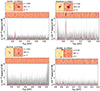 |
Fig. 1. Direct F444W stamps, Hα maps, 2D spectra, and 1D spectra of four sources in the FRESCO Hα catalog with different quality flags. Top left: single-component galaxy with q = 3. Top right: multi-component galaxy with q = 3. Bottom left: single-component with q = 2. Bottom right: single-component with q = 1. For the analysis of this paper, we only include sources with q ≥ 1.75. |
For the final Hα catalog we selected sources with an overall quality flag q ≥ 1.75, meaning that a majority of the team believed these lines to be likely real. The result is a catalog with 1050 Hα emitters: 554 from CONGRESS (in GOODS-N) and 503 from FRESCO (318 in GOODS-N and 185 in GOODS-S), with seven sources in both surveys. Despite our original S/N cut of S/N > 3 for the parent sample, all the sources flagged with q ≥ 1.75, turned out to have S/N > 5 in our final catalog.
2.4. Comparison to JADES NIRSpec catalogs
Of the sources in our Hα catalog, 123 are also present in JADES DR3 (D’Eugenio et al. 2024), which contains prism and grating redshifts for targeted sources in both GOODS fields. After comparing our grism redshifts to JADES prism redshifts, we found these to agree very well, within a scatter of 0.001 × (1 + z) and no outliers. We also compare our Hα fluxes to those of JADES DR3 in Appendix B. The grism and NIRSpec line flux measurements are broadly consistent albeit with a significant dispersion of up to 0.26 dex. While the grism data measures the full (spatially resolved) emission line without flux loss (in principle), the NIRSpec line flux measurements need to be corrected for slit losses. It is likely that this correction as well as different relative calibrations introduce this dispersion in flux measurements. Overall, this comparison is very reassuring. A more detailed comparison between the NIRSpec catalogs and the NIRCam grism line fluxes is deferred to our data release paper.
2.5. Removal of broad-line AGN
During the visual inspection process, we found 13 of our sources to show a significant broad component in their Hα lines (FWHM> 800 km s−1) consistent with AGN activity. These sources are reported in Appendix C. Eight of them are in FRESCO and match those previously reported as Little Red Dots by Matthee et al. (2024). The other five are found at lower redshifts in the CONGRESS data and are new discoveries. These sources are removed from our sample of LF measurements as we are only interested in star-forming galaxies in this work. We note, however, that our results do not change significantly with or without these sources.
2.6. UV luminosities
In order to compare our results with a different star formation rate tracer, we derive UV luminosities (and absolute magnitudes) using the fluxes in our photometric catalog. For each source, we determine which filters lie in the rest-frame UV wavelength range, i.e., 1400−2700 Å. We fit these fluxes to fν ∝ λβ − 2 by doing a linear fit in log − log space, and then interpolate the flux value at 1500 Å. This f1500; UV is then converted to LUV.
2.7. SED fitting and dust corrections
To account for dust attenuation, we fit the photometry of our sources using the Bagpipes SED fitting code (Carnall et al. 2018). We adopted a star formation history consisting of a delayed tau model and a recent burst, which we allowed to occur between 0 and 10 Myr before the time of observation. We used a (Calzetti et al. 2000) dust attenuation curve. The redshift was fixed to the grism spectroscopic redshift; however, we do not include the grism emission line fluxes in the fit. We allowed the visual attenuation to vary from AV = 0 − 5 mag, and the metallicity from Z = 0.1 Z⊙ − Z⊙, using uniform priors. Based on the resulting visual attenuation, AV, we further derive the dust attenuation at the Hα wavelength based on the Calzetti et al. (2000) curve, assuming that the nebular reddening is the same as the continuum reddening.
Of the sources in our Hα catalog, 86 have Balmer decrements measured by JADES NIRSpec spectroscopy as released in DR3 (D’Eugenio et al. 2024). JADES obtained Hα and Hβ fluxes for targeted sources in both GOODS fields using NIRSpec G140M/G235M/G395M grating and prism spectroscopy. This allowed us to compare the Hα dust attenuation, AHα, computed by Bagpipes SED fitting to that measured directly from the Balmer decrement, using the same dust attenuation law from Calzetti et al. (2000). We find that both methods provide AHα results with large uncertainties; nevertheless, the median Hα dust attenuation for the sample is consistent with both methods: AHα,med = 0.47 mag. Throughout this paper, we thus use the Hα dust attenuation values from Bagpipes derived for each source.
3. Completeness
To accurately compute luminosity number densities, we need to account for the completeness of our sample, which depends on the continuum as well as the line fluxes and the position of the sources in the field. Following each step of our catalog creation, we identify four sources of incompleteness: photometric detection, 2D spectrum extraction with grizli, line detection with grizli, and visual inspection.
3.1. Photometric detection completeness
We assess the detection completeness of the photometric catalogs following the method described in Meyer et al. (2024), which uses the GaLAxy survey Completeness AlgoRithm 2 (GLACiAR2; Leethochawalit et al. 2022). GLACiAR2 performs injection-recovery simulations by creating synthetic galaxy profiles at a range of input magnitudes and morphological parameters, injecting them at random locations in the imaging mosaics and running SourceExtractor in the same way as for the real catalog to obtain the fraction of recovered sources as a function of the observed magnitude in the detection image, magdet. As in Meyer et al. (2024), the synthetic galaxies that we generated follow a log-normal distribution centered at Reff = 0.8 kpc, which was selected to fit the morphology of our photometric catalog in F444W and F210M. The completeness is well approximated by a sigmoid function. Thus, we fit a sigmoid function to the recovered sources as a function of magdet, separately for each field, which yielded the photometric detection completeness functions, Cdet, already reported in Meyer et al. (2024) separately for GN and GS:
![Mathematical equation: $$ \begin{aligned} C_{\text{ det;GN}}&= \frac{0.95}{1 + \text{ exp}\left[1.61\times \left(\text{ mag}_{\text{ det}}-28.71\right)\right]}\quad \text{ and} \end{aligned} $$](/articles/aa/full_html/2025/02/aa52363-24/aa52363-24-eq1.gif) (1)
(1)
![Mathematical equation: $$ \begin{aligned} C_{\text{ det;GS}}&= \frac{0.93}{1 + \text{ exp}\left[1.66\times \left(\text{ mag}_{\text{ det}}-28.55\right)\right]}\cdot \end{aligned} $$](/articles/aa/full_html/2025/02/aa52363-24/aa52363-24-eq2.gif) (2)
(2)
3.2. Extraction completeness
During the line search process with grizli described in Sect. 2.2, we only considered sources with photometric redshift uncertainties of less than 20%. This constitutes a source of incompleteness, as we did not extract sources with higher uncertainties, and some of these could still be Hα emitters. As expected, most of the sources with photometric redshifts in the target range that were not extracted were among the faintest targets in the photometric catalog. To account for this, we considered all the sources with an eazy photometric redshift whose redshift probability function overlaps significantly with the grism redshift sensitivity; i.e., we consider all the sources whose lower 16th percentile fulfills zphot, 16 ≥ 3.72 (4.86) for CONGRESS (FRESCO), and zphot, 84 ≤ 5.15 (6.69) for the upper 84th percentile. We binned these sources according to their detection magnitude and calculated the percentage of sources in each bin that were extracted. We then fitted this magnitude-dependent completeness again with a sigmoid function. The result is shown separately for CONGRESS and FRESCO in Fig. 2, and the sigmoid functions that model this extraction completeness in each field are
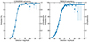 |
Fig. 2. Percentage of sources that were extracted with grizli, in detection magnitude bins. The error bars represent the binomial confidence intervals. The extraction completeness is modeled as a sigmoid function, separately for CONGRESS (left) and FRESCO (right). The resulting sigmoid functions are shown in Eqs. (3) and (4). We reach maximum completeness at mag ∼ 27. |
![Mathematical equation: $$ \begin{aligned} C_{\text{ ext;CONGRESS}}&= \frac{0.96}{1 + \text{ exp}\left[4.17\times \left(\text{ mag}_{\text{ det}}-27.82\right)\right]} \quad \text{ and} \end{aligned} $$](/articles/aa/full_html/2025/02/aa52363-24/aa52363-24-eq3.gif) (3)
(3)
![Mathematical equation: $$ \begin{aligned} C_{\text{ ext;FRESCO}}&= \frac{0.94}{1 + \text{ exp}\left[2.70\times \left(\text{ mag}_{\text{ det}}-28.09\right)\right]}\cdot \end{aligned} $$](/articles/aa/full_html/2025/02/aa52363-24/aa52363-24-eq4.gif) (4)
(4)
Both of these functions cross the 50% limit at about 28 mag.
3.3. Line detection completeness
Once the 2D spectrum of each source is extracted, we use grizli to identify emission lines and extract their properties. Our final catalog only contains sources with an Hα flux S/N > 5, as we cannot reliably confirm that lower S/N detections are genuine Hα emission lines rather than contamination. This leads to 1388 galaxies (662 in CONGRESS and 726 in FRESCO) that we are discarding, some of which might be genuine Hα emitters.
To assess this line detection incompleteness, we simulate a catalog of ∼4000 mock Hα emitters for each field and survey in a uniform grid of X and Y pixel position, emission line fluxes, and redshift. At each position, we extract the full grism spectrum (i.e., including possible contamination) and add synthetic emission lines with point source morphology. We generate synthetic emission lines for each mock source: one line of Hα (6564.59 Å), a doublet of [N II] (6549.84 Å, 6585.23 Å), and a doublet of [S II] (6718.32 Å, 6732.71 Å). The flux ratios for these five lines were set to 1 : 0.022 : 0.065 : 0.070 : 0.051. These were generated for each source in a grid of wavelength positions and log (Hα) fluxes, covering the full range of observable wavelengths (3.1 − 4.0 μm for CONGRESS; 3.9 − 5.0 μm for FRESCO) and observed Hα fluxes (8 × 10⁻¹⁹ − 8.5 × 10⁻¹⁷erg s−1 cm−2).
Finally, we used grizli to extract the mock Hα emission lines for each source and each grid combination as for real sources. If the extracted Hα line had a S/N > 5, the completeness for that grid point was assigned 1; otherwise, the completeness was 0. We combined the resulting completeness grids of all the mock sources in each field and survey by using an average of all ∼4000 grids. This led to three separate completeness functions, each depending on two variables: the wavelength (i.e., redshift) and Hα flux of the emission line. Although the completeness is also position-dependent, we marginalized over this dependence by placing sources uniformly across the FRESCO field and averaging the completeness array of all sources. These line-detection completeness functions are presented in Fig. 3. These show an asymmetric wavelength dependence due to the filter/grism throughput curve. In terms of Hα-flux level, the 50% limit is generally crossed at log(fHα/erg s−1 cm−2) ∼ −17.7, which corresponds to the FRESCO 5σ sensitivity limit of ∼2 × 10⁻¹⁸ erg s−1 cm−2 as expected from the ETC (see Oesch et al. 2023).
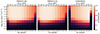 |
Fig. 3. Completeness of our line detection criteria as a function of grism wavelength (probing Hα redshift) and Hα flux, for each field and survey. Top: FRESCO GOODS-N. Middle: FRESCO GOODS-S. Bottom: CONGRESS (GOODS-N). These show an asymmetric wavelength dependence due to the sensitivity curves and cross the 50% limit at log(fHα/erg s−1 cm−2) ∼ −17.7. |
3.4. Visual inspection completeness
Due to possible contamination from other sources along the dispersion direction, grism spectra need to be visually inspected. Experienced inspectors decide whether a line is likely to be a real Hα emission line. However, some genuine emission lines might be missed during this process, due to a low S/N or the presence of contamination. To account for this visual inspection incompleteness, we selected a subsample of 320 mock Hα emitters with S/N > 5, separately for CONGRESS and FRESCO. For each survey, we selected mock sources at random pixel positions and redshifts in a grid of log(S/N). We did not cover the whole S/N range of our observations, as at the high-S/N end we found that emission lines are always properly identified during visual inspection, and thus the bright sample is complete in this sense.
We visually inspected these mock sources and gave them quality flags in the same manner as with the real data. Then, we computed the fraction of mock sources with q ≥ 1.75 in each flux bin, which correspond to the sources that would be selected into our sample if they were real. We fitted this S/N-dependent completeness with a sigmoid function. The result is shown separately for CONGRESS and FRESCO in Fig. 4, and the sigmoid functions that model this visual inspection completeness in each field are
![Mathematical equation: $$ \begin{aligned} C_{\text{ ins;CONGRESS}}&= \frac{0.90}{1 + \text{ exp}\left[15.46\times \left(\text{ log}_{10}\left(\text{ f}_{\text{ H}\alpha }\right)-0.89\right)\right]}\quad \text{ and} \end{aligned} $$](/articles/aa/full_html/2025/02/aa52363-24/aa52363-24-eq5.gif) (5)
(5)
![Mathematical equation: $$ \begin{aligned} C_{\text{ ins;FRESCO}}&= \frac{0.94}{1 + \text{ exp}\left[13.530.87\times \left(\text{ log}_{10}\left(\text{ f}_{\text{ H}\alpha }\right)-0.87\right)\right]}\cdot \end{aligned} $$](/articles/aa/full_html/2025/02/aa52363-24/aa52363-24-eq6.gif) (6)
(6)
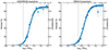 |
Fig. 4. Percentage of mock sources that were selected through visual inspection as q ≥ 1.75, in log(Hα)-flux bins. The visual inspection completeness is modeled as a sigmoid function, separately for CONGRESS (left) and FRESCO (right). The vertical dashed line marks the S/N > 5 limit. The resulting sigmoid functions are shown in Eqs. (5) and (6). |
Both of these functions cross the 50% limit at S/N ∼ 7.5.
3.5. Total completeness
The total completeness is a multiplication of the four completeness functions obtained in this section: photometric detection, extraction, line detection, and visual inspection. We compute the completeness for each source, which depends on the detection magnitude, Hα flux, line wavelength (redshift), and Hα S/N. The majority of the galaxies in our catalog have a total completeness above 65%, with only a quarter of them below this limit. In Fig. 5, we show the Hα fluxes of galaxies as a function of the detection magnitude and we highlight the sources with an estimated completeness lower than 65%. As can be seen, completeness corrections start to become significant for sources below a detection magnitude of 27 mag and for fluxes fainter than 3 × 10⁻¹⁸ erg s−1 cm−2, corresponding to log LHα/erg s−1 ≲ 41.75; MUV ≳ −20. Bins of luminosity with average completeness less than 65% are not included in the following derivations of LFs.
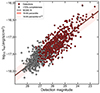 |
Fig. 5. Relation between our catalog’s Hα flux and the detection magnitude (stack of F444W and F210M). The solid, black line represents a Bayesian linear fit, while the shadowed area represents the intrinsic 1σ dispersion around the mean relation. Grey, filled circles are the sources with completeness below 65%, while red circles correspond to galaxies with higher completeness. As can be seen, our catalog of Hα emitters is starting to become incomplete at ∼3 × 10⁻¹⁸ erg s−1 cm−2, where we are likely missing emitters that are not included in our parent catalog or are not extracted due to our requirements on photo-zs. |
4. Results
4.1. Redshift distribution and overdensities
We show the redshift distribution of our Hα emitters in Fig. 6, separately for each survey and field. From CONGRESS data, we find a significant overdensity in GOODS-N at z ∼ 4.4, with 98 out of all 554 Hα emitters from the CONGRESS field lying at z = 4.43 ± 0.03. In the FRESCO fields, we find the same overdensities that were reported in Helton et al. (2024): at z ∼ 5.4 and z ∼ 5.9 in GOODS-S and a very large overdensity at z ∼ 5.2 in GOODS-N (see also Herard-Demanche et al. 2025).
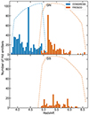 |
Fig. 6. Redshift distribution of the Hα emitters found in CONGRESS (GOODS-N) and FRESCO (GOODS-N and GOODS-S). Dashed lines show the S/N > 5 line detection completeness as a function of redshift for each survey and field. We find clear overdensities in GOODS-N at z ∼ 4.4 and z ∼ 5.2, and in GOODS-S at z ∼ 5.4 and z ∼ 5.9. |
As mentioned in Sect. 2.3, among the Hα emitters in our catalog, we found 13 sources consistent with AGN activity: five in CONGRESS and eight in FRESCO (reported in Appendix C). This constitutes a  of such sources in our catalog. For CONGRESS, four out of the five AGN candidates belong to the overdensity at z ∼ 4.4, suggesting a possible connection between AGN and larger scale environment at the 3σ level. We defer a more detailed discussion of this to a future paper.
4.2. Observed Hα luminosity function
We now compute the Hα luminosity function at 3.8 < z < 6.6. We split our full Hα catalog into three redshift bins: one for all CONGRESS data, with 3.8 < z < 5.1; and two for FRESCO data, splitting our redshift range in half: 4.9 < z < 5.7, and 5.7 < z < 6.6. We remove the broad-line Hα emitters from the luminosity function calculation, as their Hα flux does not only probe star formation (see Sect. C). This resulted in 527 CONGRESS sources at z ∼ 4.45, 379 FRESCO sources at z ∼ 5.3, and 94 FRESCO sources in the last bin centered at z ∼ 6.15.
For each redshift bin, we derive the observed Hα luminosity function following the V/Vmax method in Schmidt (1968). For each log LHα bin, we calculate the number density as
 (7)
(7)
where the summation i runs over all galaxies in the given luminosity bin, V is the full FRESCO survey volume over the redshift bin, Vmax, i is the maximum volume in which one could theoretically detect source i in that log LHα bin at redshift zi with S/N > 5, and Ci is the completeness of the source i. The uncertainty of the number density includes Poisson noise, the completeness uncertainty, as well as cosmic variance following Trenti & Stiavelli (2008), obtained with the cosmic variance calculator5. The results for a log LHα bin width of 0.25 dex are shown in Table 1 and Fig. 7. We do not consider the number density values with an average completeness below 65% for the fit, although we do show them in the figure as transparent points. We also include the dust-corrected Hα luminosity function bins in Fig. 7, which will be discussed in Sect. 4.5.
Hα luminosity functions.
 |
Fig. 7. Observed Hα luminosity function at z = 3.8 − 6.6, split in three redshift bins. Solid circles show the observed number densities, which are transparent when their average completeness is below 65% (these values are not considered for the fit). Solid lines within shaded regions show the fitted Schechter functions and the 68% confidence intervals. Also shown are the results of FLARES (Lovell et al. 2021; Vijayan et al. 2021) and SPHINX (Katz et al. 2023) at z ∼ 4, z ∼ 5, and z ∼ 6; and the results of Sun et al. (2023) at z ∼ 6.2. |
We fit a Schechter function to the observed Hα luminosity functions:
![Mathematical equation: $$ \begin{aligned} \phi =\frac{\mathrm{d}n}{\mathrm{d}\log {L}}=\ln {(10)}\,\phi ^*\,10^{\left(\log {L}-\log {L^*}\right)\,(\alpha +1)}\text{ exp}\left[10^{\left(\log L -\log L^*\right)}\right], \end{aligned} $$](/articles/aa/full_html/2025/02/aa52363-24/aa52363-24-eq24.gif) (8)
(8)
parametrized by ϕ* as the characteristic number density, L* as the characteristic luminosity, and α as the faint-end slope. To estimate these parameters, we employed a Bayesian inference approach using Markov Chain Monte Carlo (MCMC) sampling with the pymc package. We set weakly informative priors for the parameters chosen as normal distributions centered on the values found by Bollo et al. (2023) at z ∼ 4.4. We started the sampling process by finding the parameter values that maximize the posterior distribution. Subsequently, we performed MCMC sampling with 5000 iterations across four chains to obtain posterior distributions for the parameters. The posteriors were used to derive the median values and 16th–84th percentiles for each parameter, providing a comprehensive statistical characterization of the fitted Schechter function. The results of these fits are listed in Table 2 and also shown in Fig. 7.
Schechter parameters of the observed Hα luminosity functions.
4.3. Simulated Hα luminosity function
In order to compare the observed Hα luminosity functions with theoretical predictions, we added several results from simulations to Fig. 7. In particular, we use the results of the First Light And Reionization Epoch Simulations (FLARES) (Lovell et al. 2021; Vijayan et al. 2021) and SPHINX20 (Rosdahl et al. 2022), specifically the SPHINX Public Data Release v1 (SPDRv1) catalog of mock observations described by Katz et al. (2023).
While there are significant differences between the predicted LFs from these three simulations, we find decent agreement overall with our observational estimates. In particular, we find very good agreement with the predictions from FLARES, especially at the bright end. Nevertheless, in the highest redshift bin, the FLARES LF shifts towards the higher end of our fit. Interestingly, all three simulations consistently predict a higher number density of sources below our detection limit (at log LHα/erg s−1 ∼ 41.5) than the extrapolation of our derived LFs. This might indicate that our faint end slopes are somewhat too shallow and deeper observations are needed to test this. However, we note that the overall shape of our observed LFs, including the faint-end slopes, are in very good agreement with the predictions from the SC SAM model, except that they are offset by up to ∼0.3 − 0.5 dex in normalization. On the other hand, we find that SPHINX underpredicts the LF, where it overlaps with our sample, which only occurs over a very small luminosity range due to the smaller volume of SPHINX. The different results between the simulations probably stem from different approaches to the modeling of line emission, mostly separating SPHINX from FLARES and SC SAM. SPHINX can model the interstellar medium and self-consistently compute nebular emission; however, this is done at the expense of box size, which means that bright galaxies such as those observed by FRESCO and CONGRESS are rare, hence the large uncertainties in the bright end of the LF. In contrast, FLARES and SC SAM model emission lines through the use of Cloudy (Ferland et al. 1998; Chatzikos et al. 2023). Similar work in comparing high redshift line emission LFs with simulations was done by Meyer et al. (2024), who also found good agreement with FLARES and SC SAM, and that SPHINX underpredicts their values. These comparisons show that the summary statistics of emission line measurements like the LFs are a powerful new avenue to test early galaxy formation models.
4.4. UV luminosity function
Our new catalog of Hα emitters in the GOODS fields allowed us to revisit the UV LF measurements that have been performed over the last decade with photometrically selected Lyman-break galaxies, but now for the first time with spectroscopically confirmed sources. Using the same methods as in Sect. 4.2, we divided our sources into the same three redshift bins and used a MUV bin size of 0.625 mag, akin to the log LHα bin separation. The results are shown in Fig. 8, plotted together with the UV LF Schechter fits from Bouwens et al. (2021). We find that, for MUV bins where the average completeness is above 65%, our results based on spectroscopic redshifts are an excellent match, within uncertainty, to those obtained by Bouwens et al. (2021) using photometrically selected objects. This provides further confidence in the accuracy of previous UV LF measurements at these epochs.
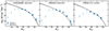 |
Fig. 8. GOODS fields UV luminosity function at z = 3.8 − 6.6, split into three different redshift bins. Solid circles show the observed number densities, which are transparent when their average completeness is below 65%. Grey lines and shaded regions are the UV luminosity functions with 68% confidence intervals obtained by Bouwens et al. (2021) for redshifts 4.45, 5.3, and 6.15, respectively. |
4.5. Star formation rate functions
The UV and Hα LFs are based on observed quantities. However, what we really would like to constrain is the buildup of star formation in early galaxies at z > 3. We can now do this based on the observed Hα emission lines, after a correction for dust extinction. To convert the Hα luminosities to SFRs, we used the relation in Kennicutt (1998), scaled by a factor of 1.8 to consider a Chabrier (2003) initial mass function (IMF):
 (9)
(9)
We computed the dust-corrected Hα luminosity using intrinsic Hα luminosities, obtained with
 (10)
(10)
where AHα is the dust attenuation at 6564.6 Å derived in Sect. 2.7. We then computed the SFR functions in the same way as the Hα LFs (see Eq. (7)). This led to the Hα-derived star formation rate functions reported in Table 3 and shown in Fig. 9. We then fitted Schechter functions to these values, using the same MCMC techniques as with the Hα luminosity function. The results of these fits are shown in Table 4.
Star formation rate functions from Hα emitters.
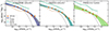 |
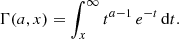
Fig. 9. Star formation rate functions at z = 3.8 − 6.6 split into three redshift bins. Solid circles show the number densities derived from dust-corrected Hα luminosities. Solid lines within shaded regions show the fitted Schechter functions and the 68% confidence intervals for Hα values. Also shown are the simulations results of FLARES (Lovell et al. 2021; Vijayan et al. 2021) and SPHINX (Katz et al. 2023) at z ∼ 4, z ∼ 5, and z ∼ 6; and the literature Hα-derived results from Bollo et al. (2023) at redshifts 3.86 < z < 4.94 and UV-derived from Smit et al. (2016) at z ∼ 3.8, 4.9, and 5.9 (scaled to match our Hα conversion factor). |
At all redshifts, we find characteristic SFRs of ∼100 M⊙ yr−1. This is significantly higher than the characteristic SFRs previously derived by Smit et al. (2016) for the SFR functions at these redshifts based on Hα lines inferred from Spitzer/IRAC broad-band photometry. We also show these estimates in Fig. 9. As can be seen, we find a significantly higher number density of galaxies with high SFRs (logSFR/M⊙yr−1 > 2) compared to the previous estimates from Smit et al. (2016). This difference is likely not the result of wrongly estimated emission line fluxes from the photometric data; it is more likely a consequence of different techniques: while we derive the SFR function directly from individual dust-corrected Hα luminosities, Smit et al. (2016) used their Hα-based SFRs to derive an average dust correction to convert the UV LFs to SFR functions. We suspect that this procedure likely underestimates the number of high-SFR sources that are present due to the significant amount of scatter in the LUV − LHα relation. Additionally, the UV-based estimates probe star formation on longer timescales than Hα, which leads to smaller dispersion. This is supported by the fact that our estimates are in very good agreement with the ones from Bollo et al. (2023) who also derived SFR functions at z ∼ 4.5 based on Hα lines inferred from Spitzer/IRAC broad-band photometry, but who used a similar procedure as we adopt here to derive the SFR functions for individual sources.
We can further compare the derived SFR functions with simulations. In particular, we have computed the SFR functions directly from the SPHINX and FLARES data. Once again, we find relatively good agreement with FLARES over most of the SFR range. Albeit, the FLARES SFR functions show a dip at SFR = 10 M⊙yr−1 at all redshifts, where their number densities are lower than what we observe by up to 0.5 dex. For the SPHINX simulation, the situation is different. While it predicts fainter Hα lines than we observe, the SFR functions are higher than what we find by more than 0.5 dex. This overestimation of the SFR function is similar to the one seen in the stellar mass function (see Weibel et al. 2024). Taken together, this likely indicates that a large amount of dust is present in the simulated galaxies, which obscures the observed quantities such as the Hα (or the UV fluxes; see also Katz et al. 2023), leading to an underpredicted Hα LF even though the intrinsic number density of galaxies at a given SFR is higher than observed.
4.6. Star formation rate densities
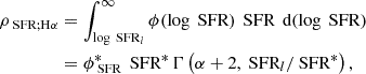
Equipped with the SFR functions derived in the previous section, we can now compute the SFRDs from our Hα measurements. We do this by integrating the SFR function, separately for each of the three redshift bins. For consistency with previous work, we set the lower integration limit to SFRl = 0.27 M⊙ yr−1, corresponding to a UV luminosity limit of MUV, l = −17. This limit was also used in Bouwens et al. (2015), that we use to compare the UV and Hα-based SFRD estimates. As the integrands are Schechter functions, we can solve these integrals analytically using:
 (11)
(11)
where Γ is the incomplete gamma function:
 (12)
(12)
For each redshift bin, we integrated each of the 5000 posterior Schechter function parameters obtained during the MCMC sampling and used the median of these results as the SFRD value, and the 16th–84th percentiles as the uncertainties.
This yields the SFRDs reported in Table 4 for each redshift bin: at z ∼ 4.45 we find 0.042 M⊙ yr−1 Mpc−3 and this declines by a factor of 3 towards z ∼ 6.15. As will be discussed in the following section, this is in good agreement with dust-corrected, UV-based measurements (e.g., Bouwens et al. 2015).
Schechter parameters of the star formation rate functions.
5. Discussion
5.1. Hα luminosity function evolution
Figure 10 shows the redshift evolution of the Hα LF across cosmic history from z ∼ 0.2 up to z ∼ 6.1 based on literature estimates as well as our new results. We observe an evolution of these luminosity functions, where z ∼ 6 galaxies are ∼1 dex less numerous than those at cosmic noon. This coincides with the epoch of galaxy buildup; hence it is expected that galaxy numbers increase with decreasing redshift. We also observe that the bright end of the Hα luminosity function is low (log(LHα/erg s−1) ∼ 42.5) at local redshifts (0.2 < z < 0.4), and it increases with redshift up to a maximum of log(LHα/erg s−1) ∼ 44 at z ∼ 2 − 3, to then decrease back to log(LHα/erg s−1) ∼ 42.5. Given that Hα is a tracer of galaxy star formation rate, this behavior agrees with the evolution shown by Madau & Dickinson (2014), where there is a peak of star formation at z ∼ 2 − 3. This is also noticeable in Fig. 11, where we compare our best-fit Schechter parameters to those of previous studies at z ∼ 0.2 − 4.4. The characteristic luminosity log L* follows the increasing trend with redshift up to z ∼ 3, to then remain fairly constant for all 4 < z < 6. Even though we note that there are degeneracies in Schechter function fits, the trends in Fig. 11 indicate that the key driver for the evolution of the Hα LFs at z < 3 is the characteristic luminosity, which then turns to an evolution in density at z > 4, i.e., the normalization parameter log ϕ* shows a slight decrease with increasing redshift, in agreement with previous results (Bollo et al. 2023).
 |
Fig. 10. Evolution of the Hα LFs across cosmic history. We compare our best-fit Hα LFs at z ∼ 4.45, z ∼ 5.3, and z ∼ 6.15, to previous results: Stroe & Sobral (2015) at z ∼ 0.2; Sobral et al. (2013) at z ∼ 0.4, 0.84, 1,47, and 2.23; Terao et al. (2022) at z ∼ 2.3; and Bollo et al. (2023) at z ∼ 4.4. Solid lines represent the regions that were probed observationally in each study. For those studies that only reported the dust-corrected luminosity functions, we inferred the uncorrected functions by reversing the dust correction applied for a fair comparison. We observe a trend of number densities increasing with decreasing redshift up to cosmic noon, to then reverse this trend and decrease until the present universe. |
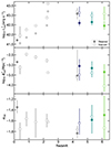 |
Fig. 11. Cosmic evolution of the Hα LF Schechter parameters. Our best-fit values are compared to previous results at lower redshifts: Stroe & Sobral (2015) at z ∼ 0.2; Sobral et al. (2013) at z ∼ 0.4, 0.84, 1.47, and 2.23; Terao et al. (2022) at z ∼ 2.3; and Bollo et al. (2023) at z ∼ 4.4. Filled circles represent the parameters of observed Hα LFs, while open circles are for dust-corrected fits. For those studies that only reported the Schechter parameters of dust-corrected measurements, we inferred the log L* parameter by reversing the dust correction applied, and show those values as fainter solid circles. |
At the same time, we do not find any significant evolution of the faint-end slope, α, with redshift, unlike for the UV luminosity functions reported by Bouwens et al. (2021), where this parameter tends to flatten with decreasing redshift, being as steep as α ∼ −2 at z ∼ 7. However, the uncertainty in our faint-end slope estimates is still very large. Deeper grism exposures will be required to constrain this better in the future, such as the ones from the ALT survey (Naidu et al. 2024).
5.2. Star formation rate density evolution
Figure 12 shows the SFRD values at various redshifts obtained from integrating the Hα luminosity functions down to SFRl = 0.27 M⊙ yr−1. For comparison, we also included values obtained from UV measurements by Bouwens et al. (2015). This provides us with a view of the star formation history of the universe at redshifts 0 ≤ z ≤ 8. We find that both Hα and UV measurements tend to lie ∼0.2 dex above the parametrization of Madau & Dickinson (2014), which was derived from UV and IR measurements prior to Bouwens et al. (2015) and integrating down to SFRl = 0.03L*. This disagreement arises from the difference between integration limits.
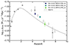 |
Fig. 12. Cosmic evolution of the SFRD. Our values compared to previous results: Stroe & Sobral (2015) at z ∼ 0.2; Sobral et al. (2013) at z ∼ 0.4, 0.84, 1.47, and 2.23; Terao et al. (2022) at z ∼ 2.3; Bollo et al. (2023) at z ∼ 4.4; and Rinaldi et al. (2023) at z ∼ 7.5. Filled circles represent values obtained from Hα luminosity functions, while open circles are from Bouwens et al. (2015) UV luminosity functions. The dotted line is the fit by Madau & Dickinson (2014). All literature results were scaled to match our Hα conversion factor. |
It is important to note that both Hα-derived and UV-derived SFRD measurements agree remarkably well with each other. Given that Hα traces star formation at much shorter timescales than UV (∼10 Myr vs. ∼100 Myr), it is common that both tracers provide different SFR values for the same galaxy due to burstiness (e.g., Cole et al. 2023; Calabrò et al. 2024; Clarke et al. 2024). Additionally, they are subject to different dust attenuation. Nevertheless, both SFRD measurements agreeing at the studied redshift range shows that these effects average out upon integration.
6. Summary and conclusions
In this work, we presented a new catalog of Hα emitters in the GOODS fields obtained using NIRCam/grism spectroscopy from JWST’s FRESCO and CONGRESS surveys. These 1050 sources entail a completeness-characterized census of line emitters at 3.8 < z < 6.6 in GOODS-North and at 4.9 < z < 6.6 in GOODS-South. With this catalog, we find a newly discovered overdensity of 98 Hα emitters in GOODS-North at z ∼ 4.4 and we confirm the overdensities reported by Helton et al. (2024). We also find five new broad Hα emitters and confirm those reported as LRDs in Matthee et al. (2024).
We computed the UV LFs and confirmed the photometry-based results from Bouwens et al. (2021) that were based on Lyman break selections. We computed the first Hα LFs at z > 3 based purely on spectroscopic data. We also derived the Hα LFs from different simulations, finding that our observed estimates are consistent with the predicted values. By comparing our observed results to previous Hα LFs over a range of redshifts, we find that both the bright and faint ends evolve from the local universe by increasing with increasing redshift up to a maximum at z ∼ 2 − 3, to then decrease back. This picture is consistent with the SFRD evolution described by Madau & Dickinson (2014), which we confirmed by obtaining three new values at redshifts 4.45, 5.3, and 6.15 from the integrated dust-corrected Hα luminosity functions. Our SFRD values agree with those derived from UV measurements, despite Hα and UV tracing star formation at different timescales.
While fitting Schechter functions to the observed Hα luminosity functions, we find a large uncertainty in the faint-end slope, α, which is also degenerate with the characteristic number density, ϕ*. This suggests that it is necessary to conduct deeper observations using NIRSpec to probe the faint end of the Hα luminosity function (as is being done with, e.g., the ALT survey). At the same time, COSMOS-3D (Kakiichi et al. 2024) and parallel programs will increase the observed area and find the most massive galaxies, probing the brighter end of the luminosity functions. Our work demonstrates the power of JWST NIRCam/grism to efficiently obtain complete emission-line-selected galaxy samples in a limited observation time (only ∼2h on source for FRESCO). In turn, these galaxy samples provide completely new constraints on galaxy formation models.
Data availability
The full Hα catalog can be found at https://github.com/astroalba/fresco
This includes partial or full coverage by the ACS F435W, F606W, F775W, F814W, and F850LP filters; the WFC3 F105W, F125W, F140W, and F160W filters; and the NIRCam F090W, F115W, F150W, F182M, F200W, F210M, F277W, F335M, F356W, F410M, and F444W filters in both fields. The GOODS-S field has additional partial coverage by the NIRCam F162M, F250M, F300M, F430M, F460M, and F480M as well as the MIRI F560W and F770W filters.
Acknowledgments
This work is based on observations made with the NASA/ESA/CSA James Webb Space Telescope. The data were obtained from the Mikulski Archive for Space Telescopes at the Space Telescope Science Institute, which is operated by the Association of Universities for Research in Astronomy, Inc., under NASA contract NAS 5-03127 for JWST. These observations are associated with program Nos. 1895 and 3577. The authors sincerely thank the CONGRESS team (PIs: Egami & Sun) for developing their observing program with a zero-exclusive-access period. We thank Aswin Vijayan and Harley Katz for their help in analyzing the simulation data from FLARES and SPHINX. This work has received funding from the Swiss State Secretariat for Education, Research, and Innovation (SERI) under contract number MB22.00072, as well as from the Swiss National Science Foundation (SNSF) through project grant 200020_207349. The Cosmic Dawn Center (DAWN) is funded by the Danish National Research Foundation under grant DNRF140. Support for program #1895 was provided by NASA through a grant from the Space Telescope Science Institute, which is operated by the Association of Universities for Research in Astronomy, Inc., under NASA contract NAS 5-03127. Support for this work for RPN was provided by NASA through the NASA Hubble Fellowship grant HST-HF2-51515.001-A awarded by the Space Telescope Science Institute, which is operated by the Association of Universities for Research in Astronomy, Incorporated, under NASA contract NAS5-26555. MS acknowledges support from the European Research Commission Consolidator Grant 101088789 (SFEER), from the CIDEGENT/2021/059 grant by Generalitat Valenciana, and from project PID2023-149420NB-I00 funded by MICIU/AEI/10.13039/501100011033 and by ERDF/EU.
References
- Bertin, E., & Arnouts, S. 1996, A&AS, 117, 393 [NASA ADS] [CrossRef] [EDP Sciences] [Google Scholar]
- Bollo, V., González, V., Stefanon, M., et al. 2023, ApJ, 946, 117 [NASA ADS] [CrossRef] [Google Scholar]
- Bouwens, R. J., Illingworth, G. D., Oesch, P. A., et al. 2012a, ApJ, 754, 83 [Google Scholar]
- Bouwens, R. J., Illingworth, G. D., Oesch, P. A., et al. 2012b, ApJ, 752, L5 [Google Scholar]
- Bouwens, R. J., Illingworth, G. D., Oesch, P. A., et al. 2015, ApJ, 803, 34 [Google Scholar]
- Bouwens, R. J., Oesch, P. A., Stefanon, M., et al. 2021, AJ, 162, 47 [NASA ADS] [CrossRef] [Google Scholar]
- Calabrò, A., Pentericci, L., Santini, P., et al. 2024, A&A, 690, A290 [NASA ADS] [CrossRef] [EDP Sciences] [Google Scholar]
- Calzetti, D., Armus, L., Bohlin, R. C., et al. 2000, ApJ, 533, 682 [NASA ADS] [CrossRef] [Google Scholar]
- Carnall, A. C., McLure, R. J., Dunlop, J. S., & Davé, R. 2018, MNRAS, 480, 4379 [Google Scholar]
- Chabrier, G. 2003, PASP, 115, 763 [Google Scholar]
- Chatzikos, M., Bianchi, S., Camilloni, F., et al. 2023, Rev. Mexicana Astron. Astrofis., 59, 327 [Google Scholar]
- Clarke, L., Shapley, A. E., Sanders, R. L., et al. 2024, ApJ, 977, 133 [NASA ADS] [CrossRef] [Google Scholar]
- Cole, J. W., Papovich, C., Finkelstein, S. L., et al. 2023, ApJS, submitted [arXiv:2312.10152] [Google Scholar]
- Cucciati, O., Tresse, L., Ilbert, O., et al. 2012, A&A, 539, A31 [NASA ADS] [CrossRef] [EDP Sciences] [Google Scholar]
- Dahlen, T., Mobasher, B., Dickinson, M., et al. 2007, ApJ, 654, 172 [Google Scholar]
- D’Eugenio, F., Cameron, A. J., Scholtz, J., et al. 2024, ApJS, submitted [arXiv:2404.06531] [Google Scholar]
- Egami, E., Sun, F., Alberts, S., et al. 2023, Complete NIRCam Grism Redshift Survey (CONGRESS), JWST Proposal. Cycle 2, ID. #3577 [Google Scholar]
- Eisenstein, D. J., Johnson, B. D., Robertson, B., et al. 2023a, ApJS, submitted [arXiv:2310.12340] [Google Scholar]
- Eisenstein, D. J., Willott, C., Alberts, S., et al. 2023b, ApJS, submitted [arXiv:2306.02465] [Google Scholar]
- Erb, D. K., Steidel, C. C., Shapley, A. E., et al. 2006, ApJ, 647, 128 [NASA ADS] [CrossRef] [Google Scholar]
- Ferland, G. J., Korista, K. T., Verner, D. A., et al. 1998, PASP, 110, 761 [Google Scholar]
- Förster Schreiber, N. M., Genzel, R., Bouché, N., et al. 2009, ApJ, 706, 1364 [Google Scholar]
- Gardner, J. P., Mather, J. C., Clampin, M., et al. 2006, Space Sci. Rev., 123, 485 [Google Scholar]
- Geach, J. E., Smail, I., Best, P. N., et al. 2008, MNRAS, 388, 1473 [NASA ADS] [CrossRef] [Google Scholar]
- Giavalisco, M., Ferguson, H. C., Koekemoer, A. M., et al. 2004, ApJ, 600, L93 [NASA ADS] [CrossRef] [Google Scholar]
- Grogin, N. A., Kocevski, D. D., Faber, S. M., et al. 2011, ApJS, 197, 2011 [Google Scholar]
- Hayes, M., Schaerer, D., & Östlin, G. 2010, A&A, 509, L5 [NASA ADS] [CrossRef] [EDP Sciences] [Google Scholar]
- Helton, J. M., Sun, F., Woodrum, C., et al. 2024, ApJ, 974, 41 [Google Scholar]
- Herard-Demanche, T., Bouwens, R. J., Oesch, P. A., et al. 2025, MNRAS, accepted [arXiv:2309.04525] [Google Scholar]
- Kakiichi, K., Egami, E., Fan, X., et al. 2024, COSMOS-3D: ALegacy Spectroscopic/Imaging Survey of the Early Universe, JWSTProposal. Cycle 3, ID. #5893 [Google Scholar]
- Kashino, D., Silverman, J. D., Rodighiero, G., et al. 2013, ApJ, 777, L8 [Google Scholar]
- Katz, H., Rosdahl, J., Kimm, T., et al. 2023, Open J. Astrophys., 6, 44 [NASA ADS] [CrossRef] [Google Scholar]
- Kennicutt, R. C., Jr. 1998, ApJ, 498, 541 [NASA ADS] [CrossRef] [Google Scholar]
- Koekemoer, A. M., Faber, S. M., Ferguson, H. C., et al. 2011, ApJS, 197, 36 [NASA ADS] [CrossRef] [Google Scholar]
- Kriek, M., Shapley, A. E., Reddy, N. A., et al. 2015, ApJS, 218, 15 [NASA ADS] [CrossRef] [Google Scholar]
- Leethochawalit, N., Trenti, M., Morishita, T., Roberts-Borsani, G., & Treu, T. 2022, MNRAS, 509, 5836 [Google Scholar]
- Lovell, C. C., Vijayan, A. P., Thomas, P. A., et al. 2021, MNRAS, 500, 2127 [Google Scholar]
- Madau, P., & Dickinson, M. 2014, ARA&A, 52, 415 [Google Scholar]
- Matharu, J., Nelson, E. J., Brammer, G., et al. 2024, A&A, 690, A64 [NASA ADS] [CrossRef] [EDP Sciences] [Google Scholar]
- Matthee, J., Mackenzie, R., Simcoe, R. A., et al. 2023, ApJ, 950, 67 [NASA ADS] [CrossRef] [Google Scholar]
- Matthee, J., Naidu, R. P., Brammer, G., et al. 2024, ApJ, 963, 129 [NASA ADS] [CrossRef] [Google Scholar]
- Meyer, R. A., Oesch, P. A., Giovinazzo, E., et al. 2024, MNRAS, 535, 1067 [CrossRef] [Google Scholar]
- Naidu, R. P., Matthee, J., Kramarenko, I., et al. 2024, Open J. Astrophys., submitted [arXiv:2410.01874] [Google Scholar]
- Nelson, E., Brammer, G., Giménez-Arteaga, C., et al. 2024, ApJ, 976, L27 [NASA ADS] [CrossRef] [Google Scholar]
- Oesch, P. A., Brammer, G., Naidu, R. P., et al. 2023, MNRAS, 525, 2864 [NASA ADS] [CrossRef] [Google Scholar]
- Oke, J. B., & Gunn, J. E. 1983, ApJ, 266, 713 [NASA ADS] [CrossRef] [Google Scholar]
- Pirie, C. A., Best, P. N., Duncan, K. J., et al. 2024, MNRAS, submitted [arXiv:2410.11808] [Google Scholar]
- Reddy, N. A., & Steidel, C. C. 2009, ApJ, 692, 778 [Google Scholar]
- Rigby, J., Perrin, M., McElwain, M., et al. 2023, PASP, 135, 048001 [NASA ADS] [CrossRef] [Google Scholar]
- Rinaldi, P., Caputi, K. I., Costantin, L., et al. 2023, ApJ, 952, 143 [NASA ADS] [CrossRef] [Google Scholar]
- Robotham, A. S. G., & Driver, S. P. 2011, MNRAS, 413, 2570 [Google Scholar]
- Rosdahl, J., Blaizot, J., Katz, H., et al. 2022, MNRAS, 515, 2386 [CrossRef] [Google Scholar]
- Schenker, M. A., Robertson, B. E., Ellis, R. S., et al. 2013, ApJ, 768, 196 [Google Scholar]
- Schiminovich, D., Ilbert, O., Arnouts, S., et al. 2005, ApJ, 619, L47 [Google Scholar]
- Schmidt, M. 1968, ApJ, 151, 393 [Google Scholar]
- Smit, R., Bouwens, R. J., Labbé, I., et al. 2016, ApJ, 833, 254 [NASA ADS] [CrossRef] [Google Scholar]
- Sobral, D., Smail, I., Best, P. N., et al. 2013, MNRAS, 428, 1128 [NASA ADS] [CrossRef] [Google Scholar]
- Steidel, C. C., Rudie, G. C., Strom, A. L., et al. 2014, ApJ, 795, 165 [Google Scholar]
- Stroe, A., & Sobral, D. 2015, MNRAS, 453, 242 [NASA ADS] [CrossRef] [Google Scholar]
- Sun, F., Egami, E., Pirzkal, N., et al. 2023, ApJ, 953, 53 [NASA ADS] [CrossRef] [Google Scholar]
- Terao, Y., Spitler, L. R., Motohara, K., & Chen, N. 2022, ApJ, 941, 70 [Google Scholar]
- Trenti, M., & Stiavelli, M. 2008, ApJ, 676, 767 [Google Scholar]
- Vijayan, A. P., Lovell, C. C., Wilkins, S. M., et al. 2021, MNRAS, 501, 3289 [NASA ADS] [Google Scholar]
- Weibel, A., Oesch, P. A., Barrufet, L., et al. 2024, MNRAS, 533, 1808 [NASA ADS] [CrossRef] [Google Scholar]
- Williams, C. C., Tacchella, S., Maseda, M. V., et al. 2023, ApJS, 268, 64 [NASA ADS] [CrossRef] [Google Scholar]
- Wyder, T. K., Treyer, M. A., Milliard, B., et al. 2005, ApJ, 619, L15 [Google Scholar]
Appendix A: Repeated sources
Within our catalog of 1050 Hα emitters, we find seven sources to show Hα emission in both FRESCO and CONGRESS surveys, two of which are multi-component. This overlap is only technically possible at 4.86 < z < 5.15, which in both surveys correspond to the edge of the grism, and thus the sensitivity at this redshift range is much lower than at the center of the grism. In fact, our seven overlapping sources are in the subrange 4.91 < z < 5.03, where there are only 17 confirmed sources in FRESCO and 21 in CONGRESS. Moreover, the overlapping sources are the brighter emitters in this redshift range, and only the fainter ones are not retrieved in the other survey, respectively.
The seven sources that we retrieve from both surveys show the same grism redshift, within a scatter of 0.05 × (1 + z), and the same flux without an offset, within 0.06σ.
Appendix B: Flux calibration
In Fig. B.1 we compare our Hα measurements to those obtained by JADES DR3 (D’Eugenio et al. 2024) for the 123 sources present in both catalogs. Our measurements were obtained with NIRCam/grism spectroscopy, while JADES DR3 used NIRSpec G140M/G235M/G395M grating and prism spectroscopy. We find a median offset on the Hα fluxes of 0.13 − 0.15 dex (calculated as log(fgrism/fJADES)), which likely arises from an undercorrection on the NIRSpec fluxes. The scatter between the two measurements is likely due to calibration differences between NIRSpec and NIRCam/grism. We find that both calibrations are consistent within 0.26(0.20)σ.
 |
Fig. B.1. Comparison between our Hα fluxes, obtained with NIRCam/grism, and the Hα fluxes in JADES DR3 (D’Eugenio et al. 2024), obtained with NIRSpec prism. The solid lines are the 1:1 relations, while the shaded regions are the 1σ deviations. The median offsets written on top are calculated as log(fgrism/fJADES). |
Appendix C: Broad Hα emitters
Upon visual inspection, we found 13 of our sources to show broad Hα lines likely consistent with AGN activity: five in CONGRESS and eight in FRESCO. The eight FRESCO sources are those reported by Matthee et al. (2024), where they have been classified as Little Red Dots, while the five sources in CONGRESS have not been reported before, and thus we performed an analysis to determine the FWHM of their broad emission. Following the procedure in Matthee et al. (2024), we fit their emission-line profiles with a combination of narrow and broad components of Hα and [N II]. We find the values reported in Table C.1. Regarding the morphology, four out of the five broad Hα emitters in CONGRESS are point-like sources, as shown on the stamps in Fig. C.1.
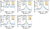 |
Fig. C.1. 1D spectra and F444W stamps of the five broad Hα emitters in CONGRESS identified in this work. Filled circles represent the observed flux values of the spectra, solid lines are the multicomponent Gaussian fits (continuum+Hα+[N II]), and dashed lines are the Hα broad, narrow, and [N II] components of these fits. The spectra are centered on the redshift of the narrow component. |
Coordinates, redshifts, and broad-component FWHM of the 13 broad Hα emitters found in this work
All Tables
Coordinates, redshifts, and broad-component FWHM of the 13 broad Hα emitters found in this work
All Figures
|
Fig. 1. Direct F444W stamps, Hα maps, 2D spectra, and 1D spectra of four sources in the FRESCO Hα catalog with different quality flags. Top left: single-component galaxy with q = 3. Top right: multi-component galaxy with q = 3. Bottom left: single-component with q = 2. Bottom right: single-component with q = 1. For the analysis of this paper, we only include sources with q ≥ 1.75. |
| In the text | |
|
Fig. 2. Percentage of sources that were extracted with grizli, in detection magnitude bins. The error bars represent the binomial confidence intervals. The extraction completeness is modeled as a sigmoid function, separately for CONGRESS (left) and FRESCO (right). The resulting sigmoid functions are shown in Eqs. (3) and (4). We reach maximum completeness at mag ∼ 27. |
| In the text | |
|
Fig. 3. Completeness of our line detection criteria as a function of grism wavelength (probing Hα redshift) and Hα flux, for each field and survey. Top: FRESCO GOODS-N. Middle: FRESCO GOODS-S. Bottom: CONGRESS (GOODS-N). These show an asymmetric wavelength dependence due to the sensitivity curves and cross the 50% limit at log(fHα/erg s−1 cm−2) ∼ −17.7. |
| In the text | |
|
Fig. 4. Percentage of mock sources that were selected through visual inspection as q ≥ 1.75, in log(Hα)-flux bins. The visual inspection completeness is modeled as a sigmoid function, separately for CONGRESS (left) and FRESCO (right). The vertical dashed line marks the S/N > 5 limit. The resulting sigmoid functions are shown in Eqs. (5) and (6). |
| In the text | |
|
Fig. 5. Relation between our catalog’s Hα flux and the detection magnitude (stack of F444W and F210M). The solid, black line represents a Bayesian linear fit, while the shadowed area represents the intrinsic 1σ dispersion around the mean relation. Grey, filled circles are the sources with completeness below 65%, while red circles correspond to galaxies with higher completeness. As can be seen, our catalog of Hα emitters is starting to become incomplete at ∼3 × 10⁻¹⁸ erg s−1 cm−2, where we are likely missing emitters that are not included in our parent catalog or are not extracted due to our requirements on photo-zs. |
| In the text | |
|
Fig. 6. Redshift distribution of the Hα emitters found in CONGRESS (GOODS-N) and FRESCO (GOODS-N and GOODS-S). Dashed lines show the S/N > 5 line detection completeness as a function of redshift for each survey and field. We find clear overdensities in GOODS-N at z ∼ 4.4 and z ∼ 5.2, and in GOODS-S at z ∼ 5.4 and z ∼ 5.9. |
| In the text | |
|
Fig. 7. Observed Hα luminosity function at z = 3.8 − 6.6, split in three redshift bins. Solid circles show the observed number densities, which are transparent when their average completeness is below 65% (these values are not considered for the fit). Solid lines within shaded regions show the fitted Schechter functions and the 68% confidence intervals. Also shown are the results of FLARES (Lovell et al. 2021; Vijayan et al. 2021) and SPHINX (Katz et al. 2023) at z ∼ 4, z ∼ 5, and z ∼ 6; and the results of Sun et al. (2023) at z ∼ 6.2. |
| In the text | |
|
Fig. 8. GOODS fields UV luminosity function at z = 3.8 − 6.6, split into three different redshift bins. Solid circles show the observed number densities, which are transparent when their average completeness is below 65%. Grey lines and shaded regions are the UV luminosity functions with 68% confidence intervals obtained by Bouwens et al. (2021) for redshifts 4.45, 5.3, and 6.15, respectively. |
| In the text | |
|
Fig. 9. Star formation rate functions at z = 3.8 − 6.6 split into three redshift bins. Solid circles show the number densities derived from dust-corrected Hα luminosities. Solid lines within shaded regions show the fitted Schechter functions and the 68% confidence intervals for Hα values. Also shown are the simulations results of FLARES (Lovell et al. 2021; Vijayan et al. 2021) and SPHINX (Katz et al. 2023) at z ∼ 4, z ∼ 5, and z ∼ 6; and the literature Hα-derived results from Bollo et al. (2023) at redshifts 3.86 < z < 4.94 and UV-derived from Smit et al. (2016) at z ∼ 3.8, 4.9, and 5.9 (scaled to match our Hα conversion factor). |
| In the text | |
|
Fig. 10. Evolution of the Hα LFs across cosmic history. We compare our best-fit Hα LFs at z ∼ 4.45, z ∼ 5.3, and z ∼ 6.15, to previous results: Stroe & Sobral (2015) at z ∼ 0.2; Sobral et al. (2013) at z ∼ 0.4, 0.84, 1,47, and 2.23; Terao et al. (2022) at z ∼ 2.3; and Bollo et al. (2023) at z ∼ 4.4. Solid lines represent the regions that were probed observationally in each study. For those studies that only reported the dust-corrected luminosity functions, we inferred the uncorrected functions by reversing the dust correction applied for a fair comparison. We observe a trend of number densities increasing with decreasing redshift up to cosmic noon, to then reverse this trend and decrease until the present universe. |
| In the text | |
|
Fig. 11. Cosmic evolution of the Hα LF Schechter parameters. Our best-fit values are compared to previous results at lower redshifts: Stroe & Sobral (2015) at z ∼ 0.2; Sobral et al. (2013) at z ∼ 0.4, 0.84, 1.47, and 2.23; Terao et al. (2022) at z ∼ 2.3; and Bollo et al. (2023) at z ∼ 4.4. Filled circles represent the parameters of observed Hα LFs, while open circles are for dust-corrected fits. For those studies that only reported the Schechter parameters of dust-corrected measurements, we inferred the log L* parameter by reversing the dust correction applied, and show those values as fainter solid circles. |
| In the text | |
|
Fig. 12. Cosmic evolution of the SFRD. Our values compared to previous results: Stroe & Sobral (2015) at z ∼ 0.2; Sobral et al. (2013) at z ∼ 0.4, 0.84, 1.47, and 2.23; Terao et al. (2022) at z ∼ 2.3; Bollo et al. (2023) at z ∼ 4.4; and Rinaldi et al. (2023) at z ∼ 7.5. Filled circles represent values obtained from Hα luminosity functions, while open circles are from Bouwens et al. (2015) UV luminosity functions. The dotted line is the fit by Madau & Dickinson (2014). All literature results were scaled to match our Hα conversion factor. |
| In the text | |
|
Fig. B.1. Comparison between our Hα fluxes, obtained with NIRCam/grism, and the Hα fluxes in JADES DR3 (D’Eugenio et al. 2024), obtained with NIRSpec prism. The solid lines are the 1:1 relations, while the shaded regions are the 1σ deviations. The median offsets written on top are calculated as log(fgrism/fJADES). |
| In the text | |
|
Fig. C.1. 1D spectra and F444W stamps of the five broad Hα emitters in CONGRESS identified in this work. Filled circles represent the observed flux values of the spectra, solid lines are the multicomponent Gaussian fits (continuum+Hα+[N II]), and dashed lines are the Hα broad, narrow, and [N II] components of these fits. The spectra are centered on the redshift of the narrow component. |
| In the text | |
Current usage metrics show cumulative count of Article Views (full-text article views including HTML views, PDF and ePub downloads, according to the available data) and Abstracts Views on Vision4Press platform.
Data correspond to usage on the plateform after 2015. The current usage metrics is available 48-96 hours after online publication and is updated daily on week days.
Initial download of the metrics may take a while.