| Issue |
A&A
Volume 699, July 2025
|
|
|---|---|---|
| Article Number | A231 | |
| Number of page(s) | 19 | |
| Section | Extragalactic astronomy | |
| DOI | https://doi.org/10.1051/0004-6361/202554618 | |
| Published online | 09 July 2025 | |
Constraints on the early Universe star formation efficiency from galaxy clustering and halo modeling of Hα and [O III] emitters
1
Cosmic Dawn Center (DAWN), Denmark
2
Niels Bohr Institute, University of Copenhagen, Jagtvej 128, 2200 Copenhagen, Denmark
3
Department of Astronomy, University of Geneva, Chemin Pegasi 51, 1290 Versoix, Switzerland
4
Institut d’Astrophysique de Paris, UMR 7095, CNRS, Sorbonne Université, 98 bis boulevard Arago, F-75014 Paris, France
5
Leiden Observatory, Leiden University, PO Box 9513 2300 RA Leiden, The Netherlands
6
Department of Astronomy and Astrophysics, University of California, Santa Cruz, CA 95064, USA
7
MIT Kavli Institute for Astrophysics and Space Research, 77 Massachusetts Ave., Cambridge, MA 02139, USA
⋆ Corresponding author: This email address is being protected from spambots. You need JavaScript enabled to view it.
Received:
18
March
2025
Accepted:
9
May
2025
Abstract
We have developed a theoretical framework that provides observational constraints on the early Universe galaxy-halo connection by combining measurements of the ultraviolet luminosity function (UVLF) and galaxy clustering via the two-point correlation function (2PCF). We implemented this framework in the FRESCO and CONGRESS JWST NIRCam/grism surveys by measuring the 2PCF of spectroscopically selected samples of Hα and [O III] emitters at 3.8 < z < 9 in 124 arcmin2 in GOODS-North and GOODS-South. By fitting the 2PCF and UVLF at 3.8 < z < 9, we inferred that the Hα and [O III] samples at ⟨z⟩∼4.3, 5.4, and 7.3 reside in halos of masses of log(Mh/M⊙) = 11.5, 11.2, and 11.0, respectively, while their galaxy bias increases with redshift with values of bg = 4.0, 5.0, and 7.6. These halos, however, do not represent extreme overdense environments at these epochs. Our framework constrains the instantaneous star formation efficiency (SFE), defined as the ratio of the star formation rate over the baryonic accretion rate as a function of halo mass. We find that the SFE rises with halo mass, peaks at ∼20% at Mh ∼ 3 × 10¹¹ M⊙, and declines at higher halo masses. The SFE-Mh shows only a mild evolution with redshift with tentative indications that low-mass halos decrease but the high-mass halos increase in efficiency with redshift. The scatter in the MUV − Mh relation, quantified by σUV, implies modest stochasticity in the UV luminosities of ∼0.7 magand is relatively constant with redshift. Extrapolating our model to z > 9 showed that a constant SFE-Mh fixed at z = 8 cannot reproduce the observed UVLF, and neither a high maximum SFE nor a high stochasticity alone can explain the high abundances of luminous galaxies seen by JWST. Extending the analysis of the UVLF and 2PCF to z > 9 as measured from wider surveys will be crucial to breaking the degeneracies between different physical mechanisms that can explain the high abundance of bright galaxies.
Key words: galaxies: evolution / galaxies: high-redshift / galaxies: luminosity function / mass function / galaxies: statistics
NASA Hubble Fellow.
© The Authors 2025
 Open Access article, published by EDP Sciences, under the terms of the Creative Commons Attribution License (https://creativecommons.org/licenses/by/4.0), which permits unrestricted use, distribution, and reproduction in any medium, provided the original work is properly cited.
This article is published in open access under the Subscribe to Open model. This email address is being protected from spambots. You need JavaScript enabled to view it. to support open access publication.
1. Introduction
One of the most pressing questions in extragalactic astronomy currently is explaining the surprisingly high abundances of bright and massive galaxies in the early Universe revealed by the James Webb Space Telescope (JWST). Statistical functions such as the ultraviolet luminosity function (UVLF) and the stellar mass function (SMF) are key observational measurements that inform models of galaxy formation and evolution in the early Universe. Measurements of both the UVLF and SMF from JWST data (e.g., Donnan et al. 2023; Harikane et al. 2023; Pérez-González et al. 2023; Bouwens et al. 2023; Finkelstein et al. 2024; Donnan et al. 2024; McLeod et al. 2024; Adams et al. 2024; Robertson et al. 2024 for the UVLF; Weibel et al. 2024; Shuntov et al. 2025; Harvey et al. 2025; Wang et al. 2024 for the SMF) have revealed galaxy abundances in excess of theoretical models and simulations calibrated on the “pre-JWST Universe” (e.g., Boylan-Kolchin 2023).
To reconcile the theory with observations, several physical mechanisms have been proposed. These can be broadly separated in two classes: (1) mechanisms that increase the star formation efficiency (SFE) in the early Universe, such as feedback-free starbursts (Torrey et al. 2017; Grudić et al. 2018; Dekel et al. 2023; Li et al. 2024; Renzini 2023), and (2) mechanisms that do not need increased SFE and can instead produce abundant bright galaxies due to increased stochasticity in the UV luminosities (Mason et al. 2023; Pallottini & Ferrara 2023; Shen et al. 2023; Gelli et al. 2024) via limited-to-no dust attenuation (Ferrara et al. 2023) or a top-heavy initial mass function (IMF, Cueto et al. 2024; Hutter et al. 2025), to name a few. The increased stochasticity manifests in the dispersion in the relation between galaxy UV magnitude (MUV) and halo mass (Mh), quantified by σUV. Bursty star formation histories naturally produce this stochasticity and have been identified both observationally via the scatter in the star forming main sequence (e.g., Ciesla et al. 2024; Clarke et al. 2024; Cole et al. 2025) and Hα-to-UV luminosity ratios (e.g., Endsley et al. 2024) as well as in simulations (Pallottini & Ferrara 2023; Sun et al. 2023; Muratov et al. 2015; Sparre et al. 2017), although halo assembly histories and varying dust attenuation can also contribute to σUV (Shen et al. 2023).
Most of these models have been developed and calibrated to reproduce one-point statistical observables such as the UVLF and the UV luminosity density. However, the galaxy-halo connection is complex (Wechsler & Tinker 2018), and there are several different mechanisms that can produce the same one-point observable, therefore making it intrinsically degenerate (Muñoz et al. 2023). Crucial information lies in how galaxies are spatially distributed, not only in how many there are. The galaxy spatial distribution, or clustering, is described by two-point statistical functions, such as the two-point correlation function (2PCF). A successful galaxy formation model has to explain both the abundances and clustering of galaxies, and therefore combining such complementary observables is key in breaking degeneracies between models (Mirocha 2020; Muñoz et al. 2023; Gelli et al. 2024).
On the observational side, using clustering as a probe alongside galaxy abundances has been done out to z ∼ 7 using Lyα emitters and Lyman-break galaxies (LBG) from Subary Suprime-Cam and Hyper Suprime-Cam (HSC) observations (Ouchi et al. 2010, 2018; Harikane et al. 2018, 2022). JWST has allowed measurements of the 2PCF out to the highest redshifts, z ∼ 10, from photometrically selected samples (Dalmasso et al. 2024a; Paquereau et al. 2025). However, JWST’s NIRCam/grism capabilities have for the first time enabled complete spectroscopically selected samples out to z ∼ 9 (e.g., Oesch et al. 2023; Kashino et al. 2023) to be compiled and their clustering (as demonstrated by Eilers et al. 2024, for a limited sample of grism-selected [O III]-emitting galaxies at 5 ≲ z ≲ 7 in a quasar field) to be measured.
On the theory side, the degeneracy issue has been explored by Mirocha (2020), Muñoz et al. (2023), who have shown that the two scenarios of high SFE versus high stochasticity that result in the same UVLF have a very distinct impact on the galaxy bias. The latter is typically measured by comparing the observed 2PCF of galaxies to the theoretical one of dark matter halos, and it describes how galaxies are preferentially distributed in the highest peaks of the underlying matter distribution. However, a comprehensive framework that models both the UVLF and 2PCF and that can be used to derive empirical constraints of the theoretical models is still lacking.
In this paper, we describe the development a theoretical framework whose purpose is to provide observational constraints on the early Universe galaxy-halo connection through the combined measurements of the UVLF and galaxy clustering via the 2PCF. This framework is based on an adaptation of the halo occupation distribution (HOD) in combination with the conditional luminosity function (CLF) and a parametric form of the SFE-Mh relation. Fitting the observed UVLF and 2PCF in an independent binning scheme allows us to provide observational constraints on the MUV–Mh and SFE-Mh relations, stochasticity, host halo masses, and galaxy bias. To implement this framework, we measured the 2PCF of spectroscopically selected samples of Hα and [O III] emitters at 3.8 < z < 9 from the JWST NIRCam/grism surveys FRESCO (Oesch et al. 2023) and CONGRESS (Egami et al. 2023).
This paper is organized as follows. Section 2 presents in detail the theoretical framework. Sect. 3 briefly presents the NIRCam/grism data and methods used to compile the line emitting samples. In Sect. 4 we describe the methods we used to measure the 2PCF and UVLF. Sect. 5 presents the results of this work. In Sect. 6 we discuss the physical implications of our results, and in Sect. 7 we summarize and conclude the paper.
We adopted a standard ΛCDM cosmology with H0 = 70 km s−1 Mpc−1 and Ωm, 0 = 0.3, where Ωb, 0 = 0.04, ΩΛ, 0 = 0.7, and σ8 = 0.82. All magnitudes are expressed in the AB system (Oke & Gunn 1983). Wherever relevant, we assumed a Salpeter (1955) IMF and rescaled the literature data points to the same IMF. The dependence of various quantities on the reduced Hubble parameter h is retained implicitly. Dark matter halo masses, scale as h−1. Absolute magnitude scale as −5 log(h) in addition. When comparing to the literature, we rescale all the measurements to the cosmology adopted for this paper.
2. Theoretical framework
We develop a theoretical framework that is based on physically motivated principles and the halo model and from which we can derive fundamental statistical observables of galaxies such as the UVLF and the galaxy correlation function. At the heart of this formalism is a parametric model of the instantaneous SFE that relates the halo accretion rate to star formation, coupled with an HOD framework to predict galaxy clustering and abundances as a function of MUV. This framework is analogous to the one developed to predict clustering and the galaxy SMF by parametrizing the stellar-to-halo mass relation (e.g., Moster et al. 2010; Leauthaud et al. 2011, 2012; Shuntov et al. 2022). The novelty of this work is the extension to the UVLF, which also sets it apart from other works that use the 2PCF in combination to the total number density of MUV-threshold selected galaxies (e.g., Harikane et al. 2018, 2022).
2.1. The ultraviolet luminosity to halo mass relationship
Galaxy star formation and mass growth is directly connected to the growth rate of dark matter halos since the gas available for star formation is well mixed with the dark matter with a ratio of fb ≈ 0.16 (e.g., Moster et al. 2018; Tacchella et al. 2018). This relation can be written as
 (1)
(1)
The halo accretion rate, Ṁh, is well understood from ΛCDM, and we took the Dekel et al. (2013) form as a function of halo mass and redshift. The star formation rate Ṁ⋆ is moderated by the instantaneous SFE, ϵ. This function encapsulates all baryonic physics responsible for regulating star formation in halos and is essentially a summary of our galaxy formation model. Typically, it depends on both redshift and halo mass ϵ(z, Mh), and we adopted the double power law parametrization as a function of Mh (Moster et al. 2010, 2018):
![Mathematical equation: $$ \begin{aligned} \epsilon (M_{\rm h}) = 2\, \epsilon _0 \left[ \left(\dfrac{M_{\rm h}}{M_c}\right)^{-\beta } + \left(\dfrac{M_{\rm h}}{M_c}\right)^{\gamma } \right]^{-1}. \end{aligned} $$](/articles/aa/full_html/2025/07/aa54618-25/aa54618-25-eq2.gif) (2)
(2)
This relation has four free parameters: ϵ0, the normalization or the peak SFE; Mc, a characteristic halo mass at which the efficiency peaks; and β and γ, respectively the low- and high-mass slopes. In our implementation, we model these parameters as a function of redshift and fit for their redshift dependence (following e.g., Moster et al. 2018; Muñoz et al. 2023, more details in Sect. 4.3).
We note here that Eq. (1) is distinct from the integrated SFE, ϵ⋆, that has been used frequently in recent high-z literature (e.g., Behroozi & Silk 2018; Boylan-Kolchin 2023). The latter quantifies the ratio between the stellar and halo mass assembled throughout the history of a halo,  , also known as the stellar-to-halo mass relationship (SHMR, Wechsler & Tinker 2018). The two are related by a time integral and do not necessarily have the same normalization and shape (Behroozi et al. 2013; Moster et al. 2018), unless ϵ is Universal and time independent. In this paper, we mainly work with the instantaneous SFE (ϵ), and refer to it whenever we discuss the SFE, unless we state otherwise (e.g., if we refer to the integrated SFE)
To arrive at the UV luminosity, we used the fact that the SFR and UV luminosity are related with the luminosity-to-SFR conversion factor κUV:
 (3)
(3)
Here, κUV is fully degenerate with ϵ0 (Muñoz et al. 2023), but in a first and simplistic approach we assumed its fiducial value  for a Salpeter IMF (Madau & Dickinson 2014). From the luminosity, we then derived the absolute magnitude MUV in the AB system in the following way:
 (4)
(4)
Finally, we added dust by using the AUV − β relation from Meurer et al. (1999) and β − MUV from Bouwens et al. (2014) and following the implementation in Mason et al. (2015), Sabti et al. (2022) and references therein. This assumes that β follows a Gaussian distribution at each MUV with a dispersion of σβ = 0.34. The average dust extinction is then ⟨AUV⟩ = 4.43 + 0.79 ln(10) σβ + 1.99 ⟨β⟩.
Equations (1)–(4) relate the UV luminosity, MUV, to the halo mass, Mh, resulting in a MUV–Mh relationship, or UVHMR, which we denote as fUVHMR(Mh). MUV has a monotonically increasing relation with Mh that depends on redshift (e.g., Mason et al. 2015). The exact dependence is shaped by the change of both halo growth and the instantaneous SFE with time.
2.2. The conditional ultraviolet luminosity function
The MUV–Mh is not a one-to-one relation and there is a scatter in MUV at a given Mh. This can be modeled by a CLF, which gives the average number of galaxies with MUV ± dMUV/2 in a halo of mass Mh (Yang et al. 2003, 2009). This can be modeled as a Gaussian distribution with a scatter σUV:
![Mathematical equation: $$ \begin{aligned} P(M_{\rm UV}|M_{\rm h}) = \dfrac{1}{\sqrt{2\,\pi }\,\sigma _{\rm UV}} \mathrm{exp}\left[ -\left( \dfrac{M_{\rm UV} - f_{\rm UVHMR}(M_{\rm h})}{\sqrt{2} \, \sigma _{\rm UV}} \right)^2 \right], \end{aligned} $$](/articles/aa/full_html/2025/07/aa54618-25/aa54618-25-eq7.gif) (5)
(5)
where fUVHMR(Mh) gives the average MUV as a function of halo mass Mh. The scatter σUV is not only a result of intrinsic astrophysical processes, σUV, intr but also of observational uncertainties in measuring MUV, σUV, meas (Leauthaud et al. 2011), which can be written as σUV2 = σUV, intr2 + σUV, meas2. Additionally, σUV can be a function of halo mass (e.g., Sun et al. 2023; Gelli et al. 2024), however in our implementation in this paper we simplify it and neglect this dependence on Mh.
2.3. The halo occupation distribution
The CLF, crucially, provides a link to the HOD framework, which describes the statistical occupation of galaxies in dark matter halos and provides a formalism to model galaxy clustering via the two-point correlation function (e.g., Cooray & Sheth 2002; Berlind & Weinberg 2002). The HOD is a prescription of the mean number of galaxies residing in a halo of mass Mh, which is given as
![Mathematical equation: $$ \begin{aligned} \left\langle N_{\rm tot}\left(M_{\rm h}\right) \right\rangle = \left\langle N_{\rm cent}\left(M_{\rm h}\right) \right\rangle \times \left[1 + \left\langle N_{\rm sat}\left(M_{\rm h}\right) \right\rangle \right]. \end{aligned} $$](/articles/aa/full_html/2025/07/aa54618-25/aa54618-25-eq8.gif) (6)
(6)
It is made of two components describing the mean occupation numbers of central and satellite galaxies. The occupation function for central galaxies brighter than some threshold luminosity,  , can be derived by integrating the CLF
 (7)
(7)
Carrying out this integration and accounting for the fact that MUV is negative, we arrived at
![Mathematical equation: $$ \begin{aligned} \left\langle N_{\rm cent}\left(M_{\rm h} | M_{\rm UV}^\mathrm{th}\right) \right\rangle = \dfrac{1}{2} \left[ 1 - \text{ erf} \left( \dfrac{f_{\rm UVHMR}(M_{\rm h}) - M_{\rm UV}^\mathrm{th}}{\sqrt{2}\,\sigma _{\mathrm{UV}}} \right) \right]. \end{aligned} $$](/articles/aa/full_html/2025/07/aa54618-25/aa54618-25-eq11.gif) (8)
(8)
We can obtain this functional form by analytically integrating Eq. (7), thanks to the Gaussian form of P(MUV|Mh) and because we assumed a constant σUV. In principle, it is possible to allow a functional form of σUV with Mh and to carry out the integration of Eq. (7) numerically to obtain ⟨Ncent⟩.
The occupation of halos by satellites can be modeled by a power-law for which we adopted the Zheng et al. (2005) form
 (9)
(9)
where Mcut and Msat are the minimum and characteristic halo masses necessary to host satellite galaxies, and αsat is the power-law slope. This is different from other implementations of this formalism, where the satellite occupation is modeled by a combination of power- and exponential-law (Leauthaud et al. 2011; Coupon et al. 2015; Shuntov et al. 2022). We opted for this simpler description in order to reduce the number of free parameters.
The average number of galaxies in a UV luminosity bin of  can also be computed by simply taking the difference of the occupation numbers for two MUV thresholds
 (10)
(10)
2.4. Model of the galaxy ultraviolet luminosity function
Having a description of the mean occupation numbers of galaxies as a function of their MUV and of their host halo mass Mh, we can derive an analytical form for the UVLF by simply integrating over the halo mass function in the following way
 (11)
(11)
Here,  indicates that the UVLF is computed for a MUV bin defined by the two thresholds
  and
and  . For the integration limits, in practice we adopt the [106 − 1015] M⊙ range. dn/dMh is the halo mass function (HMF), for which we use the code COLOSSUS (Diemer 2018), with the Watson et al. (2013) HMF and virial overdensity halo mass definition.
2.5. Model of the two-point correlation function
The model of the two-point angular correlation function follows closely the usual prescriptions (see, e.g., Cooray & Sheth 2002). For completeness, we detail the principal equations in Appendix D. For the computation of the 2PCF, we rely on the HALOMOD1 code (Murray et al. 2013, 2021). HALOMOD is a library of routines to calculate a range of cosmological observables. The main ingredients that enter the modeling along with the prescriptions and assumptions that we adopt are given in Table 1.
Adopted ingredients in the halo model.
One of the ingredients in computing the 2PCF is the halo bias, which describes how halos trace the underlying dark matter distribution. Analytical forms of the halo bias are typically calibrated in the linear regime and on large scales using N-body simulations. However, not accounting for non-linear and scale-dependent effects fails to accurately describe the ‘quasi-linear’ regime of the one-halo to two-halo transition (r ∼ 10 − 500 kpc) and can underpredict galaxy clustering by up to 30% (Reed et al. 2009; Jose et al. 2013; Mead et al. 2015; Jose et al. 2016; Mead & Verde 2021). As demonstrated in more detail in Harikane et al. (2018), Paquereau et al. (2025), accounting for non-linear and scale-dependent bias becomes important in accurately modeling the observed 2PCF at z ≳ 3. To deal with this, we use the same implementation as in Paquereau et al. (2025), based on the Jose et al. (2016) non-linear scale-dependent corrections. Finally, we also apply the halo-exclusion correction that accounts for the fact that halos cannot overlap and supresses the two-halo power at scales smaller than the halo size (Zheng 2004; Tinker et al. 2005).
2.6. Derived parameters
Using the mean halo occupation numbers and the halo mass function, we can derive various parameters related to the DM halos. The number density of galaxies predicted by the HOD model is computed as
 (12)
(12)
The average mass of the DM halo of galaxies at a given redshift is
 (13)
(13)
The mean galaxy bias at a given redshift is
 (14)
(14)
where bh(Mh, z) is the Tinker et al. (2010) linear halo bias.
2.7. Ultraviolet luminosity function, two-point correlation function, and galaxy bias dependence on model parameters
In Fig. A.1 we show how the UVLF, 2PCF and galaxy bias change with different model parameter values. This demonstrates which measurements are most constraining for the model parameters. For this we adopt a set of fiducial parameter values σUV = 0.76, ϵ0 = 0.22, log Mc = 11.56, β = 0.69, γ = 0.74, log Mcut = 8.99, log Msat = 12.69, αsat = 0.76, and we vary each parameter at a time, shown in the different rows in Fig. A.1.
The UVLF is most sensitive to the parameters that govern instantaneous SFE ϵ(Mh) and σUV. The scatter, σUV, mostly affects the bright end, such that a higher scatter flattens the bright-end slope, resulting in higher abundances of bright (MUV < −21) galaxies. Correspondingly, this reduces the clustering amplitude and galaxy bias. Increasing the maximum SFE, ϵ0 effectively shifts the UVLF toward the brighter end while decreasing the 2PCF amplitude and bias. This happens because higher efficiencies mean that lower mass halos, that are less clustered, can host brighter galaxies. The peak halo mass Mc governs the location of the ‘knee’ of the UVLF with higher values moving the knee toward the brighter end, while increasing the 2PCF amplitude. The slopes β and γ affect the faint and bright end respectively, where increasing β, increases the 2PCF, while γ has very little impact on the 2PCF. The parameters governing the satellite occupation (Msat, Mcut, αsat) have negligible impact on the UVLF and bias, but affect mostly the smaller scales of the 2PCF (one-halo term).
2.8. Advantages and caveats
The theoretical framework we developed for this work is highly flexible in modeling galaxy observables under a common parametrization of the instantaneous SFE, the MUV − Mh scatter, and the satellite occupation numbers. These model parameters can in turn be parametrized with redshift. This is a powerful approach that allows modeling of the UVLF at any redshift bin under the same model parameters and consistently incorporates different z-bins under the same likelihood. Furthermore, this method allows for an independent binning scheme for the 2PCF and UVLF measurements. In fact, this is how we implemented this framework in this paper (see Sect. 4.2).
Furthermore, this framework is highly modular – the same parametrization can be used to model additional statistical observables such as the SMF. This observable is complementary to the UVLF and subject to different systematics and therefore can be a powerful addition to help break degeneracies and better constrain the model. We will explore this in a future work.
As detailed in Sect. 2.1, the modeling includes a number of assumptions that can introduce systematic biases. For example, assumptions of the UV luminosity-to-SFR conversion factor κUV and the dust attenuation relations can be degenerate with the model parameters (we discuss this further in Sect. 6). Furthermore, there is also a degeneracy with the duty cycle that gives the fraction of galaxies that are UV-bright at a given moment (e.g., Mirocha 2020; Muñoz et al. 2023). The duty cycle can be incorporated in the model by a multiplying the total occupation number Ntot fduty (e.g., Harikane et al. 2016) and would result in scaling the 2PCF and UVLF differently (Mirocha 2020; Muñoz et al. 2023, provide details on how exactly it affects the UVLF and galaxy bias). For example, lowering fduty would require increasing ϵ0 to match the UVLF, but would decrease the 2PCF amplitude. We assume a duty cycle of unity, consistent with indications from previous work (Harikane et al. 2018, 2022; Muñoz et al. 2023). Future work including larger datasets would allow us to model the duty cycle, which can even be a function of halo mass (e.g., Ouchi et al. 2001; Mirocha 2020).
3. Data
This work is anchored on the most comprehensive and complete JWST NIRCam/grism spectroscopic surveys – FRESCO (Oesch et al. 2023) in the F444W filter and CONGRESS (Sun, Egami et al. in prep., Egami et al. 2023) in the F356W. These two surveys cover the 3.1 − 5.0 μm range over 62 arcmin2 in GOODS-North. In addition, FRESCO covers another 62 arcmin2 in GOODS-South at 3.8 − 5.0 μm. Combined, these enable the compilation of complete samples of Hα emitters at 3.7 < z < 6.7 (4.9 < z < 6.7) in GOODS-North (GOODS-South), and [O III] emitters at 6.8 < z < 9.
We used the samples compiled by the works of Covelo-Paz et al. (2025, for Hα emitters) and Meyer et al. (2024, for [O III] emitters). We describe them briefly here but refer the reader to these references for more details. Photometric catalogs in the GOODS fields are extracted using all publicly available HST (e.g., Giavalisco et al. 2004; Grogin et al. 2011; Koekemoer et al. 2011, in ten bands) and JWST (e.g., Eisenstein et al. 2023a,b; Williams et al. 2023, in 11 bands (19 for GOODS-S). Detection is carried out on an inverse-variance stack of the F210M and F444W bands from FRESCO to ensure homogenous depth. Source extraction is done with SEXTRACTOR (Bertin & Arnouts 1996) on images that were PSF-matched to the F444W band. Aperture corrections are applied to scale the fluxes to those measured in Kron apertures on a PSF-matched version of the detection image, and then to total by dividing by the encircled energy of the Kron aperture on the F444W PSF. The detection completeness is estimated using the GLAC IAR2 software (Leethochawalit et al. 2022) by measuring the fraction of injected-recovered sources as a function of F444W magnitude. The completeness is constant around 90% out to 27 AB mag and declines to zero out to 30.5 AB mag. The NIRCam WFSS data is reduced and processed using the GRIZLI software using the standard CRDS grism dispersion files from pmap 1123 (Oesch et al. 2023; Meyer et al. 2024). In the following, we briefly describe the selection of Hα and [O III] emitters.
3.1. Hα sample
The Hα sample is constructed by first selecting all sources with Hα S/N > 3 from the GRIZLI catalog. Multi-component sources are identified upon visual inspection and components within < 0.6 arcsec separation and identical grism redshifts are merged into one galaxy and assigned the same Hα line. Quality flags are assigned via visual inspection by four team members independently. We use quality flag q ≥ 1.75, which means that the source has a clear Hα line and a matching morphology between the direct image and the 2D-spectrum and the line map, or a lower S/N but a clear morphology map. Additionally, a high quality flag is assigned for FRESCO Hα emitter at z > 5.25 that show a [O III] emission from the CONGRESS data (Covelo-Paz et al. 2025).
3.2. [O III] sample
The [O III] sample is constructed by requiring S/N ≥ 3 in F444W FRESCO band and no detection in bands blueward of Lyman-α to remove unambiguous low-z contaminants. Then, for all these sources, the 1D spectra are filtered with a Gaussian with FWHM = 50, 100, 200 km s−1 and candidates are retained if they satisfy the following conditions: (1) Two lines match the [O III]λλ5008,4960 Å separation at 6.8 < z < 9.0, with a tolerance of Δν < 100 km s−1 on the doublet separation, (2) S/N> 4 for the strongest line of the doublet, (3) The observed doublet ratio 1 <[O III]5008/[O III]4960 < 10. Visual inspection is carried out by multiple team members independently to remove contaminants and assign quality flags (q), similarly to the Hα catalog. We use objects with q ≥ 1.5, which is slightly less conservative than for the Hα sample; we opt for this lower value to maximize the number of objects for this intrinsically smaller sample of [O III] emitters (Meyer et al. 2024).
3.3. Selection function
The selection described above yields emission line-selected samples in three redshift bins – two Hα emitter samples, the first at 3.7 < z < 5.1 from CONGRESS, the second at 4.9 < z < 6.7 from FRESCO, and a third sample of [O III] emitters at 6.8 < z < 9. We apply a cut in the UV absolute magnitude to select only sources with MUV < −19.1. This threshold is chosen as the brightest magnitude that selects enough sources to allow measurement of the 2PCF w(θ). Practically, this requires that there is at least one pair of objects at the angular separations θ at which w(θ) is evaluated using the Landy & Szalay (1993) estimator (Sect. 4.1, Eq. (15)).
This selection function results in 398 galaxies for the 3.7 < z < 5.1 Hα CONGRESS sample, 387 galaxies for the 4.9 < z < 6.7 for the Hα FRESCO sample, and 108 galaxies for the 6.8 < z < 9 [O III] sample. Figure 1 shows the spatial and redshift distributions of the three samples in the GOODS-North and GOODS-South fields.
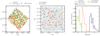 |
Fig. 1. Spatial distribution of the three line-emitting samples (Hα and [O III] from FRESCO and Hα from CONGRESS) in the GOODS-North and GOODS-South footprints (left and middle panels) that we consider in this analysis. The right panel shows their redshift distribution. The density histogram gray background in the left and middle panels shows the footprint of the random catalogs. |
4. Measurements
4.1. Galaxy clustering via two-point angular correlation function
We measure galaxy clustering via the angular 2PCF, for the three emission line-selected samples, brighter than MUV = −19.1 mag, in the three redshift bins, using the Landy & Szalay (1993) estimator2. We measured the 2PCF using Eq. (15) for GOODS-North and GOODS-South separately and combined them together using a number density weighting scheme following Durkalec et al. (2015)
 (15)
(15)
where DDi, RRi, and DRi are the number of data-data, random-random, and data-random pairs in a given angular separation bin [θ, θ + δθ] normalized by the total number of galaxies and random objects for each field i = 1, 2. In addition, wi = (Ni/Vi)2 is the weight defined as the total number of galaxies divided by the volume of the corresponding field.
We constructed random catalogs for the two fields and the two samples by Monte-Carlo sampling of the LF (Hα and [O III] accordingly) to assign a line flux to each random source. To account for the fact that the spatial selection function can be wavelength dependent we use the root-mean-square (RMS) cube given in Meyer et al. (2024) along with the completeness functions for the [O III] and Hα samples (Meyer et al. 2024; Covelo-Paz et al. 2025). We compute the S/N for each source as a function of position and wavelength and retain the random draw with a probability equal to the completeness as a function of S/N. This ensures that the random catalog accounts for any spatial selection effects in the data.
Given the fact that this is a sample with highly precise redshifts from spectroscopy, it is in principle possible to compute the projected correlation as a function of comoving perpendicular separation wp(rp). However, our samples are too small to carry out the measurement of wp(rp) that is not too noisy for model fitting, and therefore we use the projected angular correlation function w(θ) for our analysis. This is also consistent with the predictions by Endsley et al. (2020) using mock galaxy samples based on the UNIVERSEMACHINE model.
Uncertainties in the 2PCF measurements come from Poisson pair-counting statistics and from cosmic variance (Norberg et al. 2009). The latter can have important impact on the measurements, especially for small field-of-view surveys like FRESCO. One way to estimate the cosmic-variance uncertainties is via jackknife, bootstrapping or Monte Carlo methods (Norberg et al. 2009, 2011). However, the small number of sources and footprint render jackknife and bootstrapping methods unsuitable, while Monte Carlo methods would require cosmological simulations and synthetic galaxy catalogs, which is expensive and out of the scope of this work. Furthermore, using such simulations, Leauthaud et al. (2011) showed that cosmic variance has an impact on the covariance matrix on large scales (i.e., in the two-halo regime) – it increases the correlation in the data at large scales, which is poorly constrained with our measurements due to the relatively small field.
We adopt a simplistic approach by considering only Poisson uncertainties, boosted by 30% in quadrature. We estimated the 30% cosmic variance uncertainty using the galcv calculator (Trapp et al. 2022) for the survey volume apparent magnitude of our sample. Additionally, we tested a more conservative boost of 10% and verified that it does not impact the results significantly. Because of the small sample, it is also difficult to derive well-defined covariance matrices that are not too noisy for likelihood computation. For this reason, we use only the diagonal elements, and therefore not consider the covariance between different θ bins (commonly adopted in the literature in case of small samples, e.g., Zehavi et al. 2011).
Due to the small volume probed in the GOODS-North and GOODS-South fields, the integral constraint (IC) suppresses/cuts w(θ) at scales near and beyond the survey size. We took this into account by adjusting the model with a correction factor that can be estimated from the double integration of the true correlation function over the survey area:
 (16)
(16)
This integration can be carried out using the random-random pairs from the random catalog following Roche & Eales (1999)
 (17)
(17)
where wtrue(θ) comes from the HOD-predicted model. Finally, the model that we fit against the data is simply w(θ) = wtrue(θ)−wIC.
4.2. Ultraviolet luminosity functions
Since our Hα and [O III] samples are identical to those used in Covelo-Paz et al. (2025) and Meyer et al. (2024), we take the UVLF measurements presented in the respective papers. The completeness-corrected UVLFs are measured for the Hα CONGRESS at z ∼ 4.3, Hα FRESCO in two bins at z ∼ 5.3 and z ∼ 5.6, and the [O III] sample in two bins at z ∼ 7.1 and z ∼ 7.2. The advantage of these UVLFs is that they are measured from secure spectroscopic samples, therefore alleviating systematic biases that can arise from typical photometrically selected samples. These are shown as yellow/red symbols in Fig. 3.
However, these samples are limited at both the bright and faint end due the survey volume and sensitivity limits. In order to gain significant constraining power from the UVLFs, we also adopt the measurements from Bouwens et al. (2021) that use photometrically selected LBG over 1136 arcmin2. We use the UVLFs in five bins at z ∼ 4, 5, 6, 7, 8 shown in gray symbols in Fig. 3. As described in Sect. 2.4, our highly flexible modeling allows us to simultaneously model all of these ten UVLFs consistently and include them under the same likelihood. Finally, we boost the UVLF errorbars to account for about 25% of cosmic variance uncertainty (e.g., Trapp et al. 2022; Sabti et al. 2022).
4.3. Fitting procedure
We fit the measurements in all redshift bins simultaneously by assuming a parametric redshift dependence of the model parameters. In this way, we model a smooth redshift evolution of ϵ(Mh, z). We adopted a linear dependence with redshift for all parameters following Muñoz et al. (2023)
 (18)
(18)
where X = [ϵ0, log Mc, β, γ, σUV, log Mcut, log Msat,αsat].
We fit the models of the w(θ) and the UVLFs to our measurements using a Markov chain Monte Carlo (MCMC) approach while minimising χ2:
 (19)
(19)
where the w terms are the measurement vectors containing w at θ, and  and
and  are the models for a given set of parameter values. The first term of Eq. (19) corresponds to the clustering likelihood and the second term to UVLF likelihood. The sums run over the different measurements in the three redshift bins for the clustering and ten in total UVLFs at different redshifts (five for the line-emitter samples and five for the LBG).
We carried out the fitting using the EMCEE code (Foreman-Mackey et al. 2013), that implements an affine-invariant ensemble sampler. We used 50 walkers for our five parameters and relied on the auto-correlation time τ to assess the convergence of the chain. To consider the chains converged, we require that the auto-correlation time is at least 50 times the length of the chain and that the change in τ is less than 1%. We discard the first 2 × max(τ) points of the chain as the burn-in phase and thin the resulting chain by 0.5 × min(τ). We impose flat priors on all parameters; for the mass parameters, the flat priors are on the log quantities.
For best-fit parameter values, we take the medians of the resulting posterior distribution, with the 16th and 84th percentiles giving the lower and upper uncertainty estimates. We compute the confidence intervals on all HOD model-derived quantities by computing it from 500 randomly drawn samples from the posterior, and taking the 1σ percentiles. The posterior median and 1σ uncertainties of the main model parameters X are given in Table B.1, for the three redshift bins of the Hα and [O III] samples. We also present the values for the parameters describing the linear with redshift dependence (Eq. (18)).
5. Results
5.1. Clustering of Hα and [O III] emitters
We measured galaxy clustering via the angular 2PCF for spectroscopically selected galaxies out to z ∼ 4.3 and z ∼ 5.4 for Hα emitters, and z ∼ 7.3 for [O III] emitters brighter than MUV = −19.1 mag. These are shown in Fig. 2. The high resolution in NIRCam allowed us to probe very small scales deep into the one-halo regime, down to about 10 kpc at z ∼ 6; however, the limited survey area prevents us from probing scales larger than ∼1 Mpc at z ∼ 6.
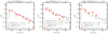 |
Fig. 2. Angular 2PCF measured from the Hα CONGRESS and FRESCO samples at z ∼ 4.3 and z ∼ 5.4 and [O III] sample at z ∼ 7.3 selected at MUV < −19.1 mag. Comparison with literature measurements includes Harikane et al. (2022), Dalmasso et al. (2024a), and Paquereau et al. (2025) for samples selected at similar redshifts and MUV as our work. |
The amplitude of the 2PCF for the Hα emitters increases mildly from z ∼ 4.3 to z ∼ 5.4, and continues to increase for the [O III] emitters at z ∼ 7.3. The shape of the 2PCF for the three samples resembles a power law, in contrast to the characteristic two-component behavior of the one- and two-halo terms. This is not surprising, given the fact that this is the regime where the non-linear scale-dependent bias can amplify the power at intermediate ∼100 − 500 kpc scales (Jose et al. 2017). Furthermore, relatively low-number statistics prevent us from accurately revealing the shape of the 2PCF for these samples. Finally, cosmic variance systematics (e.g., overdensities in the field) can have an influence on both the shape and amplitude of the 2PCF. Indeed, recent spectroscopic redshift searches for overdensities in the GOODS fields have revealed several significant overdensities at z ∼ 6 − 7 (Helton et al. 2024; Meyer et al. 2024; Covelo-Paz et al. 2025; Herard-Demanche et al. 2025).
In Fig. 2, we also show a comparison with recent measurements from the literature. Dalmasso et al. (2024a) measure clustering of LBG in the JADES survey, and as such their sample overlaps with ours. We compare with their measurements at z ∼ 5 and z ∼ 7, but for fainter samples than ours with mean UV magnitudes of ⟨MUV⟩∼ − 19.2, compared to ours ⟨MUV⟩∼ − 20. In general, there is good agreement, with differences that are likely due to the redshift and MUV selection; for example, at z ∼ 7 our 2PCF has expectedly larger amplitude because of brighter sample. Harikane et al. (2022) measure the 2PCF of photometrically selected LBG in the HSC Subaru Strategic Program (SSP) survey over ∼300 deg2 at 4 < z < 7. There is relatively good agreement with slightly higher amplitude of their brighter, MUV ≲ −20 sample, compared to our MUV < −19.1 mag sample. Finally, we find excellent agreement with Paquereau et al. (2025) measurements in the ∼0.5 deg2 COSMOS-Web survey for stellar mass selected samples of log(M⋆/M⊙) > 8.5. This is comparable to our MUV threshold of −19.1 mag assuming the Song et al. (2016) mass-to-light ratio. Slight differences likely arise from the redshift selection.
This consistency of the 2PCF with the literature is indeed reassuring and showcases that photo-z selected samples can yield robust and unbiased 2PCF, with an advantage of compiling significantly larger samples than what is possible with spec-z. This means that future implementation of our modeling framework will be possible using 2PCF measured from photo-z selection, therefore reducing errorbars and extending the analysis to z > 9.
5.2. UVHMR × HOD model fitting
We implemented the theoretical framework presented in Sect. 2 to fit simultaneously the measurements of the 2PCF in the three redshift bins (Sect. 4.1, Sect. 5.1) and the ten UVLFs across the 3.8 < z < 9.0 range (Sect. 4.2). In Fig. 3 we show the resulting median (solid lines) and 1σ uncertainty (envelope) computed from sampling the posterior distribution of the model parameters. The top row shows the best-fit models of the 2PCF, while the bottom row shows those of the UVLF at the mean redshift of the corresponding bin (e.g., ⟨z⟩∼4.3, 5.4 and 7.3). We show only one UVLF model for clarity, while in Fig. C.1 we show the individual fits for each measurement.
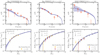 |
Fig. 3. Best-fit models of the 2PCF and UVLF. Top row: Angular 2PCF measured from the Hα CONGRESS and FRESCO samples at z ∼ 4.3 and z ∼ 5.4 and [O III] sample at z ∼ 7.3 (orange points). Bottom row: UVLF for the same line emitter samples from Covelo-Paz et al. (2025), Meyer et al. (2024) along with the photometrically selected samples from Bouwens et al. (2021). The blue curves and envelopes show the median models and 1σ uncertainty computed from the posterior. In the case of the UVLF, for simplicity we show only the models in the same redshift bins as the 2PCF measurements. We show the individual fits for each measurement in Fig. C.1. |
The models show good fits of the data within the uncertainties for the 2PCF and UVLFs for all redshifts. In the case of the 2PCF, at the intermediate scales around the one-halo to two-halo transition (θ ∼ 10″) the data show slightly higher amplitudes than the data, likely due to imperfect modeling of the non-linear and scale-dependent halo bias (see Sect. 2.5). The overall good fit showcases that our framework can successfully model both the UVLF and 2PCF and derive physical insights, which we present in the following.
5.3. Mean halo mass and galaxy bias
The HOD modeling of the 2PCF and UVLF allowed us to infer the mean mass of the DM halo that hosts our line emitter samples and their bias (Sect. 2.6). Figures 4 and 5 show the mean halo mass and galaxy bias for the Hα samples at z ∼ 4.3 and 5.4 and [O III] at z ∼ 7.3.
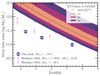 |
Fig. 4. Mean halo mass for the three line emitter samples: Hα samples at z ∼ 4.3 and 5.4 and [O III] at z ∼ 7.3 with MUV < −19.1 mag. We compare with measurements from Harikane et al. (2016) and Harikane et al. (2022) for photometrically selected LBG. The colored regions are derived from the EVS (Lovell et al. 2023) formalism and indicate the confidence intervals to observe the most massive halo in the GOODS volume (2 × 60 arcmin2) within the ΛCDM model. The dotted line marks the median of the EVS distribution of the maximum plausible halo mass. |
This analysis shows that the line emitters samples from our work are hosted in halos of log(Mh/M ,
,  ,
,  for the Hα and [O III] samples at z ∼ 4.3, 5.4 and 7.3 respectively. These halos are less massive by ∼0.2 dex compared to those hosting similarly bright LBG from the Harikane et al. (2016) analysis.
We interpreted the derived halo masses with the extreme value statistics (EVS; Lovell et al. 2023) formalism. EVS is a probabilistic approach to estimating the PDF of observing the most massive halo at a given redshift and given cosmological volume. In Fig. 4 we show the confidence intervals of the PDF
 derived from EVS for our GOODS area (2 × 60 arcmin2). The masses of the halos hosting our line emitter samples are lower than the most massive halo expected in GOODS by ∼0.7 dex. This is unsurprising, given the fact that we measure the mean halo mass hosting a sample of normal, star-forming galaxies with MUV < −19.1 mag. We note that the Harikane et al. measurements are made in a much larger volume of the HSC-SSP and are not comparable with these EVS intervals derived for GOODS.
In Fig. 5 we show the galaxy bias as a function of redshift and MUV. The blue empty circles correspond to the bias for the three line emitter samples at the corresponding median redshift. We measure a galaxy bias of  ,
,  ,
,  , for the Hα and [O III] samples at z ∼ 4.3, 5.4 and 7.3 respectively. Since we fit the continuous redshift dependence of our model, we can derive the redshift evolution of the galaxy bias as a function of MUV. This is shown in the blue lines in Fig. 5; however, we note that this is an extrapolation beyond the z and MUV regime we probed in our work. Our results show that the bias increases with both redshift and luminosity, as expected from the theory (e.g., Kaiser 1984). Our measurements are comparable those of similarly bright LBGs from Dalmasso et al. (2024a). The stellar mass selected sample of Paquereau et al. (2025) also shows comparable values for the bias, although slightly elevated (by ≲1) at 5 < z < 8. This can be due to differences in the redshift and MUV selection as well as in the modeling.
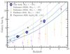 |
Fig. 5. Galaxy bias as a function of redshift and MUV. The empty circles with error bars show the bias for the three line emitter samples Hα at z ∼ 4.3 and 5.4, and [O III] at z ∼ 7.3 with MUV < −19.1 mag. The solid blue lines show the bias as a function of redshift for four MUV thresholds computed from our model. We compare with measurements from Harikane et al. (2016), Dalmasso et al. (2024b) and Dalmasso et al. (2024a) for photometrically selected LBG, as well as Paquereau et al. (2025) for stellar mass selected, normal galaxies. |
5.4. Ultraviolet magnitude-halo mass relation
Our framework allows us to measure the MUV − Mh relationship (UVHMR) and its evolution with redshift. In Fig. 6 we show our results on the UVHMR at the median redshifts of our three line emitters samples. However, in principle, since we fit for the redshift evolution of our model parameters, we have information of the continuous evolution of the UVHMR over the redshift range that we probe in this work, as well as extrapolations beyond. In this work, we only probe a limited range in MUV and correspondingly in Mh with the 2PCF, which is marked by the solid lines and bold envelopes in Fig. 6. The transparent envelopes extend to the minimum MUV that is probed by the UVLF. We show the dust-attenuated MUV.
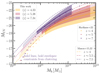 |
Fig. 6. Relationship of MUV − Mh (or UVHMR) for the redshift bins of our three line emitter samples. The solid lines and bold envelopes mark the MUV range that we probe with the 2PCF, while the transparent envelopes mark the range probed by the UVLF. We compare with the model by Mason et al. (2015, 2023) that includes dust attenuation in dashed lines and the observational measurements from Harikane et al. (2022) in dots. |
The UVHMR shows the typical monotonic increase of UV luminosity with increasing Mh. As the halo mass increases, the slope of the UVHMR decreases, with a pivot mass at Mh ∼ 3 × 10¹¹ M⊙. This is a similar pivot mass scale as the galaxy SHMR (Wechsler & Tinker 2018). The UVHMR evolves with redshift such that halos of fixed mass host brighter galaxies at earlier epochs. The high mass and luminosity end becomes shallower at lower redshifts due to the more important effect of dust attenuation. The relatively large uncertainties prevent us from inferring any potential mass or luminosity dependence of the redshift evolution.
We compare our measurements with the theoretical model from Mason et al. (2015, 2023) and the observational measurements from Harikane et al. (2022), which also include dust-attenuation. In the MUV and Mh regime probed by our work, our UVHMR shows shallower slopes for all redshift bins, indicating luminosities that increase faster with halo mass. At fainter luminosities, the constraints from UVLF-only are in better agreement with the Mason et al. (2015, 2023) model.
5.5. The instantaneous star formation efficiency
The central feature of our modeling is the parametric form of the instantaneous SFE, and its dependence on halo mass and redshift, ϵ(z, Mh) (Eq. (2)), that we constrain from observations of the UVLF and 2PCF. As a reminder, ϵ is defined as the ratio between the SFR and the halo accretion rate times the universal baryon fraction  (Eq. (1)), and describes the efficiency of converting gas to stars.
Figure 7 shows our results on the SFE as a function of halo mass for the three redshift bins of our three line emitter samples. The solid lines and bold envelopes indicate the MUV (and correspondingly Mh) range probed with the 2PCF, while the transparent envelopes mark the range probed by the UVLF. We note that the upper Mh range is derived from the MUV–Mh relation, and it can extend to halo masses beyond the maximum mass expected in the GOODS volume, as indicated in Fig. 4. Therefore, we caution the interpretation of these results at the highest masses that can be considered as extrapolation.
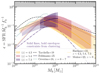 |
Fig. 7. Star formation efficiency as a function of halo mass for the redshift bins of our three line emitter samples. The solid lines and bold envelopes mark the MUV range that we probe with the 2PCF, while the transparent envelopes mark the range probed by the UVLF. We compare with the observational measurements using 2PCF and HOD from Harikane et al. (2022) in dotted lines, empirical model by Tacchella et al. (2018) in dashed line, and results from cosmological simulations by Ceverino et al. (2024) and Feldmann et al. (2025) in solid colored lines. |
The SFE shows the characteristic dependence with halo mass – increasing up to a peak halo mass scale of Mh ∼ 3 × 10¹¹ M⊙ and decreasing for halos more massive than this peak mass. This characteristic shape of the SFE-Mh relation is typically explained by the effect of stellar and AGN feedback suppressing star-formation at the low- and high-mass end (e.g., Silk & Mamon 2012).
As a function of redshift, our results show very little evolution in the 4 ≲ z ≲ 7 range. At the low-mass end (Mh < 2 × 10¹¹ M⊙) the SFE shows a decrease by about 0.3 dex from z ∼ 4.3 to z ∼ 7.3. However, at the high-mass end (Mh > 1012 M⊙) there are tentative indications that the trend is reversing, and the SFE increases with redshift, albeit with large uncertainties. This trend becomes clearer when we look at the redshift dependence of the best-fit parameters in Fig. 8. The normalization of the SFE, ϵ0, shows a mild increase with redshift with a positive slope  . However, the lower uncertainty limit is also consistent with zero slope, therefore making it difficult to draw a robust conclusion. The peak mass scale, Mc, also increases with redshift with a slope
  , meaning that the SFE shifts toward high masses, which creates the decrease of the SFE with redshift at the low-mass end. The high-mass end slope γ decreases (
 ), causing the SFE to increase with redshift at a fixed halo mass larger than Mc. This suggests increasing efficiencies of more massive halos in the early Universe. However, this remains a tentative interpretation, given the fact that the 1 σ upper limit on dγ/dz is also consistent with an increasing slope. Additionally, the increase of Mc with redshift is primarily driven by the measurements in the z ∼ 7.3 bin, where the 2PCF is relatively noisy. As shown in Fig. A.1, lower clustering amplitude would lower Mc. These uncertainties highlight the need for larger galaxy samples for more precise clustering measurements in order to conclusively infer the redshift evolution (or lack thereof) of the SFE.
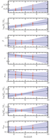 |
Fig. 8. Resulting values of the model parameters. These values were obtained by drawing 1000 samples from the posterior and evaluating the models at a given z using Eq. (18). The orange points and errorbars mark the redshift bins of the 2PCF measurements. The dashed lines mark the z-parametrized functions (Eq. (18)) for our model parameters, evaluated at the median posterior. |
We compare our results with the observational measurements using the 2PCF and HOD modeling from Harikane et al. (2022), the empirical model by Tacchella et al. (2018) and the results from the cosmological simulations FIRSTLIGHT (Ceverino et al. 2024) and FIREBOXHR (Feldmann et al. 2025). Our analysis is closest to that of Harikane et al. (2022) and the SFE is in relatively good agreement in a 1 dex range around the peak halo mass. At lower (< 1011 M⊙) and higher (> 1012 M⊙) halo masses, our measurements indicate higher and lower SFE, correspondingly. The Tacchella et al. (2018) empirical model assumes a universal SFE constant with redshift and has a lower peak halo mass by about 0.2 − 0.3 dex and higher efficiencies at < 3 × 10¹¹ M⊙. Compared to the cosmological simulations, Feldmann et al. (2025) find a non-evolving SFE in FIREBOXHR, although they can only probe the very low mass end due to the limited simulation volume. Their results are in close agreement to ours at z ∼ 4.3, with the difference that our results indicate a mild redshift evolution. Additionally, the slope of their SFE−Mh relation is considerably shallower and can have important implications for derived galaxy statistical quantities such as the UVLF and the SFR density, which we discuss in Sect. 6. On the other hand, Ceverino et al. (2024) find a SFE that evolves with redshift in FIRSTLIGHT. Their SFE in the only overlapping z = 6 − 7 bin shows elevated efficiencies compared to ours by about 0.2 − 0.4 dex, with an indication of a peak occurring at a similar halo mass scale.
6. Discussion
6.1. Stochasticity versus star formation efficiency
Crucially, our model allows us to break the degeneracy between the high SFE versus high stochasticity scenarios by quantifying both ϵ and σUV observationally. In the following, we discuss the implications of our measurements on these two scenarios.
Our results indicate that there is some level of stochasticity, described by modest values of the scatter σUV ∼ 0.65. From our measurements in 4 ≲ z ≲ 8 range, we find that σUV remains roughly constant with redshift with a slope  . In Fig. 9 we show the redshift evolution of σUV inferred from our work and compared with the literature. We show in blue points with errorbars our measurements at the mean redshifts of the three line emitter samples. The blue solid line and envelope show the best-fit and 1σ uncertainty as a linear function of redshift. We note that beyond z ≳ 8 these are extrapolations since we do not include any observational (UVLF) constraints.
Compared to the literature, there is a relatively good agreement out to z ∼ 9 from independent approaches. Muñoz et al. (2023) fit the UVLF with a similar modeling and find consistent values with ours. Their linear with redshift parametrization of σUV is also consistent with our measurement. However, when they fit for independent z-bins they find that σUV needs to increase sharply at z > 10 to fit the observed JWST UVLFs, a regime currently unconstrained by our framework.
Indeed, there is observational evidence that the transition from secular to stochastic star formation occurs at z ≳ 6 − 9 (Ciesla et al. 2024; Cole et al. 2025; Endsley et al. 2024; Looser et al. 2025; Dressler et al. 2023; Langeroodi & Hjorth 2024). Ciesla et al. (2024), for instance, study SF histories and show that at z ∼ 9 about 87% of massive galaxies have evidence for a stochastic star formation in the last 100 Myr, while only 15% at z < 7. However, this is not reflected in the redshift independent σUV ∼ 1.2 that they infer (filled squares in Fig. 9). This is likely due to the different definition of σUV which is simply the MUV dispersion computed from SED fitting of their sample. Additionally, they estimate σUV in an alternative way by decomposing it into different components and using the SFR-M⋆ dispersion, and find σUV ∼ 0.68, in agreement with our results (empty squares in Fig. 9). However, we note that σUV (i.e., the scatter in UV magnitude at a given halo mass) that we analyze in our work is not directly comparable with empirically measured values of SF burstiness, usually derived from ratios of SFR from emission lines and UV continuum and/or non-parametric SFH modeling.
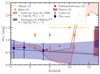 |
Fig. 9. Scatter in the MUV−Mh relation, represented as σUV, as a function of redshift. The blue points with errorbars mark σUV at the median redshift of our three line emitter samples, while the blue line and envelope mark the best-fit and 1σ uncertainty as a linear function of redshift. From the literature compilation, the colored boxes at the right axis show the σUV for a range of Mh independent of redshift from the FIRE and FIREBOXHR simulations (Sun et al. 2023; Feldmann et al. 2025). For Muñoz et al. (2023), we show the 1σ contours for σUV obtained for independent z-bin fits; while the dashed purple line shows their best-fit linear function with redshift. For Ciesla et al. (2024) we show results from two different methods in the filled and empty squares. |
In the cosmological hydrodynamical simulations FIRE-2 (Sun et al. 2023) and FIREBOXHR (Feldmann et al. 2025), σUV is a decreasing function of Mh in the range ∼1.40 − 0.35 at 9 < log(Mh/M⊙) < 12 for FIRE-2, and ∼1.55 − 0.70 at 9 < log(Mh/M⊙) < 11 for FIREBOXHR, both independent of redshift. These are indicated in the colored boxes on the right axis of Fig. 9. Our results align well with these simulations, as our sample primarily resides in halos with 11 < log(Mh/M⊙) < 11.5 (see Sect. 5.3), a halo mass regime that would correspond to similar σUV values in the simulations. Finally, in the SERRA simulation Pallottini & Ferrara (2023) find a σUV at z ∼ 7.7 consistent with ours (diamond symbol in Fig. 9).
Gelli et al. (2024) discuss the physical motivations behind a halo mass and redshift dependent σUV. Under the assumption that the stochasticity is driven by the ability of halos to retain the gas despite the feedback processes, then it would scale inversely to the escape velocity, i.e.,  . This would mean σUV decreases with redshift, which is qualitatively consistent with our measurement of
  .
.
Our work adds further observational evidence that stochasticity alone cannot explain the observed UVLFs and galaxy clustering measured via the 2PCF out to z ∼ 9. However, the regime in which there is some disagreement with the literature remains at z > 9, where the transition to stochastic SF is identified. For example, at the highest redshifts (z > 10 − 16) Shen et al. (2023) and Kravtsov & Belokurov (2024) find that values as high as σUV ∼ 2 are required to explain the observed UVLF. This is also found by Muñoz et al. (2023) as mentioned earlier. This redshift regime is beyond the scope of this work, but future application of our framework to larger datasets extending to z > 9 promises to provide valuable observational constraints.
We carried out a simple exercise using our theoretical framework to investigate the high stochasticity versus SFE scenarios at z > 9. We use the model parameters at z = 8 which corresponds to the upper redshift limit of our data, and compute the UVLF at z > 8. Since the parameters fix the HOD at z = 8, this means that the redshift evolution is primarily driven by the HMF evolution. Figure 10 shows the UVLF predictions from our model in solid lines, and compared to measurements from the literature (symbols). Unsurprisingly, at z ≥ 9 our model consistently underpredicts the observed UVLF with the difference increasing with redshift.
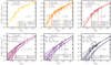 |
Fig. 10. Predictions of UVLF out to z = 13 from our model constrained on z < 8 data and compared to measurements from the literature. The solid lines correspond to the model evaluated at different redshifts from the best-fit linear redshift dependence of the model parameters fit on 4 ≲ z ≲ 8 data. The dashed and dotted lines illustrate the two extreme scenarios of increasing SFE versus increasing stochasticity and show the model where we tune by hand ϵ0 and σUV to approximately match the observations, while keeping the other parameters nominal. The filled area shows the effect of dust attenuation on the UVLF, with the upper thin lines marking the unatenuated UVLF. |
We note that in simply increasing ϵ0, our empirical modeling remains agnostic about other physical mechanisms that can be triggered by increasing the SFE. These include stellar feedback, gas ejection, accretion modulation, increase in metallicity and dust content, which can act to suppress the SFE and impact the resulting UVLF. In this sense, the SFE that we assume by increasing ϵ0 should be considered as the effective SFE that encapsulates all the effects triggered by the increase in ϵ0. However, since our modeling is agnostic to these, the derived UVLF are more consistent with upper limits.
We illustrate how two extreme cases would fit the UVLF. One case involves increasing only the maximum SFE ϵ0, and the second involves increasing only the stochasticity via σUV. We tuned both parameters by hand at each z to roughly match the UVLF while keeping the other parameters to their nominal values (e.g., Fig. 8). At z = 10, ϵ0 ∼ 35% (compared to the nominal value of ∼25%) would be required to match the UVLF in the first case, while the second case requires σUV = 1.1, which is almost double the nominal. At the highest redshifts, z ≥ 12, both cases require extreme values, increasing ϵ0 to ∼95% and σUV to ∼1.8.
This exercise shows that neither of the two scenarios alone is likely to explain the observed UVLFs, since they require extreme values for ϵ0 and σUV. Such values are typically not predicted by current simulations, although some models (e.g., feedback-free starbursts; Torrey et al. 2017; Grudić et al. 2018; Dekel et al. 2023; Li et al. 2024; Renzini 2023) can produce such high efficiencies. However, taken together, the impact of different SFEs, and plausible increases in stochasticity, may well result in those high abundances of luminous galaxies. Therefore, the solution is likely a contribution from both the stochasticity and the SFE along with its dependence on halo mass (e.g., Gelli et al. 2024). A mass dependence of σUV that we neglect in our work can have important contributions, but since our framework allows us to implement a halo mass dependence, we will explore this in future work.
To highlight the importance of the SFE dependence on halo mass, we can compare with the results by Feldmann et al. (2025) based on the FIREBOXHR simulation. They find that a non-evolving, weakly mass dependent SFE (shown in Fig. 7) can explain the observed UV luminosity density at z > 10. The reason for this is the shallow slope of their SFE-Mh relation at 9 < log(Mh/M⊙) < 11 that increases the contribution from the more numerous lower mass halos at higher redshifts – this can integrate the UVLF to the observed values. This suggests that the global SFE in low-to-intermediate mass halos are higher than previously determined empirically (e.g., Tacchella et al. 2018; Harikane et al. 2022) or in simulations such as FIRSTLIGHT (Ceverino et al. 2024). Compared to these models, our empirical results also show shallower SFE-Mh slopes at the low-mass end, but slightly steeper than Feldmann et al. (2025), which given the steep increase of the HMF at low masses, could be sufficient to explain why our SFE cannot reproduce the observed UVLF, and correspondingly the UV luminosity density at z > 10.
Higher SFE due to a shallow SFE-Mh slope at low-to-intermediate masses is certainly one viable explanation for the observed abundances of bright galaxies at z > 10. However, it remains to be tested against other galaxy observables such as the 2PCF and SMF and extended at log(Mh/M⊙) > 11. Indeed, the high-mass regime can be crucial in revealing the full picture. For example, in our case the mild decrease of the SFE with z at the low-mass end is balanced by an increase at the high-mass end and this kind of evolution explains both the 2PCF and UVLF at 4 < z < 8. The importance of the bright and massive end in constraining the models and distinguishing between physical mechanisms at z > 10 is illustrated in Fig. A.1 in the context of the SFE model parameters and σUV. Figure A.1 shows that at z ∼ 6, varying ϵ0 = 0.2 ± 75% changes Φ [Mpc−3 mag−1] by ∼2 dex at MUV = −22 mag, but < 1 dex at MUV = −19 mag. Similarly, variation of σUV = 0.6 ± 75% results in ΔΦ [Mpc−3 mag−1]∼2.5 dex at MUV = −22 mag, but only ∼0.2 dex at MUV = −19 mag.
We can conclude from this that it is important to determine the SFE in a large Mh range, spanning several orders of magnitude and beyond the characteristic halo mass of ∼1012 M⊙ at different epochs in order to understand its (non)evolution with redshift. This can be made possible by implementing our framework to wider and deeper surveys to probe the bright and faint end accordingly, in a wedding-cake approach that can include the whole JWST extragalactic surveys archive. This is necessary in order to provide suffficiently large samples for clustering measurements as well as robust measurements of the bright end of the UVLF.
6.2. Model degeneracies and how to break them
The framework that we developed in this work is highly predictive, but relies on several physical assumptions that can be degenerate. However, our framework is flexible enough to be extended to model and constrain these against additional observables.
As mentioned in Sect. 2, the luminosity-to-SFR conversion factor κUV is fully degenerate with the maximum SFE, ϵ0 (Inayoshi et al. 2022; Muñoz et al. 2023; Shen et al. 2023). This means that it is effectivelly the ϵ0/κUV ratio that determines the inferred SFE, when constrained against the UVLF. However, κUV might not remain universal at all epochs. For example, different IMF assumption can change κUV from 1.15 × 10⁻²⁸ (M⊙ yr−1)/(erg s−1), for a Salpeter IMF (adopted in this work) to κUV to 0.72 × 10⁻²⁸ (M⊙ yr−1)/(erg s−1), for a Chabrier IMF (Madau & Dickinson 2014). Additionally, lower metallicities and/or top-heavy initial mass functions, as expected for Population III stars, can result in an even lower κUV (e.g., Bromm et al. 2002; Inayoshi et al. 2022), that would drive ϵ0 down in order to reproduce the same UVLF. Finally, κUV depends also on the duration of the previous star formation (Wilkins et al. 2019) and on the age of the stellar population, which can also change at earlier times.
This has been implicitly explored in Donnan et al. (2025) who assume an integrated SFE3 constant with time, tuned to reproduce the SMF at z ∼ 7, and fit for a M⋆ − MUV relationship that fits the UVLF at 6 < z < 13. The changing mass-to-light ratio evokes younger and thus brighter stellar populations at earlier times which effectively tweaks κUV toward lower values (κUV ∝ 1/LUV), while forcing ϵ0 constant. This showcases the ϵ0/κUV degeneracy.
Stellar masses and SMFs provide complementary probes that can help break this degeneracy because they do not depend on κUV. This is shown by the fact that the stellar mass is a result of the integrated SFR times a mass loss function4,  . This also means that the SMF can be modeled under the same parametrization as the UVLF and the 2PCF. M⋆ being independent of κUV means that the SMF can break the ϵ0/κUV degeneracy. However, observational stellar mass estimates depend on the IMF assumption during SED fitting (e.g., Conroy et al. 2009) which can complicate this application.
The SMF is an important probe to consider because accurate measurements of the instantaneous SFE need to be able to reproduce the observed SMF. In the context of the SMF, it is the integrated SFE,  , that describes the relationship between the galaxy stellar mass and host halo mass (SHMR). The SHMR has been found to show some level of evolution with redshift by numerous works in the past (e.g., Conroy & Wechsler 2009; Behroozi et al. 2010; Moster et al. 2010, 2013; Behroozi et al. 2019; Girelli et al. 2020; Shuntov et al. 2022). Additionally, recent measurements from JWST at z ≳ 7 using abundance matching and HOD analysis show an important evolution toward high efficiencies at early times (Shuntov et al. 2025; Paquereau et al. 2025). This seems in contrast with the indications of a very mild evolution of the instantaneous SFE. This suggests that additional modeling components and observational probes (such as the SMF) need to be incorporated in order to accurately inform our models and break degeneracies such as ϵ0/κUV and σUV. Therefore, we identify that the way forward in unveiling a complex picture of intertwined processes is constraining physical models on several complementary probes including the 2PCF, UVLF, SMF and potentially others.
Finally, negligible dust attenuation in the early Universe can also be responsible for the observed abundances of bright galaxies (Ferrara et al. 2023; Mason et al. 2023). In our work we used the canonical AUV − β (Meurer et al. 1999) and β − MUV (Bouwens et al. 2014) relations to attenuate the MUV when fitting the observed UVLFs, and extrapolating to predict the UVLF at z > 9. However, this is uncertain because there is evidence from JWST that the β − MUV relationship ma changes toward bluer β slopes at z > 8 (e.g., Cullen et al. 2023; Topping et al. 2024), indicating negligible dust attenuation, as well as indications of the opposite (e.g., Saxena et al. 2024). We showcase the effect of dust attenuation on the UVLF in Fig. 10 with the filled areas, where the upper thin lines mark the unatenuated UVLF. This makes it clear that the level of dust attenuation adds additional degeneracy in the models. Interestingly, in the case of very high stochasticity, the attenuation in the UVLF appears to be negligible. This is unsurprising, because low luminosity galaxies scattered in high-mass halos will indeed have little attenuation. Incorporating the SMF in our formalism would allow for relaxing of the assumptions of dust attenuation and for them to be fit directly. However, the difficulty of measuring accurate stellar masses at high redshift is likely to limit that application.
7. Conclusions
In this paper, we have presented a theoretical framework developed to combine measurements of UVLF and galaxy clustering via the 2PCF into a probe of the galaxy-halo connection. We based this powerful framework on the CLF in order to model the UV luminosity–halo mass relationship (which we called UVHMR) in combination with the HOD. It is a highly flexible adaptation of the HOD framework that allows for the use of independent redshift binning schemes for each probe (UVLF and 2PCF) and parametrizes with redshift the model parameters. As such, when fit on the UVLF and 2PCF, it provides empirical constraints on the redshift evolution of the SFE-Mh and MUV–Mh relationships, stochasticity, host halo masses, and galaxy bias. Importantly, this formalism allows for the incorporation of independent probes to test and break degeneracies between different physical models proposed to explain the surprising abundances of bright and early galaxies seen by JWST.
To implement this framework, we measured the 2PCF of spectroscopically selected Hα and [O III] line emitters from FRESCO and CONGRESS JWST NIRCam/grism surveys in 124 arcmin2 in the GOODS-North and GOODS-South fields. Our UVHMR×HOD modeling successfully fit the 2PCF and UVLF measurements in three and ten redshift bins at 3.8 < z < 9, respectively. Our main findings are summarized as follows:
-
The clustering of MUV < −19.1 mag Hα and [O III] emitters shows 2PCF amplitudes in agreement with similarly bright LBG and normal galaxy samples from the literature. The 2PCF amplitude increases mildly from z ∼ 4.3 to z ∼ 7.3, and the shape resembles a power law, thus requiring modeling the non-linear scale-dependent halo bias in order to boost the amplitude at quasi-linear scales (∼100 − 500 kpc).
-
The dark matter halos that host the Hα and [O III] samples at z ∼ 4.3, 5.4, and 7.3 have mean masses of log
 ,
,  , and
, and  , respectively. The galaxy bias increases with redshift with values of
  ,
,  ,
,  for the three samples, showing that these galaxies reside in high peaks of the underlying matter density field. However, EVS analysis revealed that their host halos do not correspond to extreme overdense environments for their respective epochs.
 -
The SFE-Mh relation rises gradually with halo mass, peaks at about 20% at Mh ∼ 3 × 10¹¹ M⊙, and declines at higher halo masses. The SFE-Mh shows only a mild evolution with redshift and tentative indications that low-mass halos decrease but the high-mass halos increase in efficiency with increasing redshift. However, uncertainties are large and consistent with no evolution scenario.
-
The scatter in the MUV–Mh relationship, quantified by σUV, suggests a modest stochasticity of ∼0.7. σUV is constant with redshift and in agreement with the literature out to z ∼ 9.
-
Extrapolating our model at z > 9 shows that a constant SFE−Mh fixed at z = 8 cannot reproduce the observed UVLF. A high maximum SFE or high stochasticity alone cannot explain the high abundances of luminous galaxies seen by JWST since they require extreme and unlikely values (e.g., ϵ0 ∼ 0.95, σUV ∼ 1.8). Additionally, negligible dust attenuation can result in an up to 0.5 − 1 dex increase of the abundance of luminous galaxies. Therefore, it is not implausible that the combination of high SFE, high stochasticity, and low dust attenuation could conspire to create galaxy formation events that differ from what is seen at later times, resulting in an unexpected abundance of highly luminous galaxies at early times.
Extending this analysis to z > 9 and including additional and complementary probes will be crucial in constraining the galaxy-halo connection and revealing the dominant physical mechanisms in early star formation. Judging from the consistency of our spec-z selected 2PCF measurements with the photo-z selected measurements from the literature, it is promising that photo-z selected samples throughout all JWST surveys will provide sufficiently large samples for 2PCF and UVLF measurements out to the highest redshifts (consistent with the predictions from mocks by Endsley et al. 2020). This will be possible because photometric selection allows for the selection of fainter samples, which are more numerous. However, survey width will also be crucial in constraining the UVLF and clustering of bright galaxies for which the model parameters are more sensitive and can thus shed light on the underlying physical mechanisms.
Data availability
To make our results transparent and facilitate comparison we provide all our measurements which can reproduce the figures in this paper in tabulated form at https://github.com/mShuntov/Clustering_and_HOD_of_Ha-and-OIII_emitters. and https://zenodo.org/records/15386639
The correlation functions are computed using the TREECORR code (Jarvis et al. 2004).
Synonymous with the SHMR (Sect. 2.1).
We note that this is a different estimate from, for example, via stellar population synthesis techniques, which require an IMF and therefore depend on κUV.
Acknowledgments
This work is based on observations made with the NASA/ESA/CSA James Webb Space Telescope. The raw data were obtained from the Mikulski Archive for Space Telescopes at the Space Telescope Science Institute, which is operated by the Association of Universities for Research in Astronomy, Inc., under NASA contract NAS 5-03127 for JWST. Some of the data products presented herein were retrieved from the Dawn JWST Archive (DJA). DJA is an initiative of the Cosmic Dawn Center, which is funded by the Danish National Research Foundation under grant No. 140 (DNRF140). This work was made possible by utilizing the CANDIDE cluster at the Institut d’Astrophysique de Paris, which was funded through grants from the PNCG, CNES, DIM-ACAV, and the Cosmic Dawn Center and maintained by S. Rouberol. We thank Giorgos Nikopoulos for kindly sharing a neat UVLF literature compilation. We thank Anne Hutter for the valuable discussions. This work has received funding from the Swiss State Secretariat for Education, Research and Innovation (SERI) under contract number MB22.00072, as well as from the Swiss National Science Foundation (SNSF) through project grant 200020_207349. This work was further supported by funding from JWST-GO-01895, provided through a grant from the STScI under NASA contract NAS5-03127. This work made use of the following Python packages: numpy (Harris et al. 2020), matplotlib (Hunter 2007), scipy (Virtanen et al. 2020), astropy (Astropy Collaboration 2022), HALOMOD (Murray et al. 2021)
References
- Adams, N. J., Conselice, C. J., Austin, D., et al. 2024, ApJ, 965, 169 [NASA ADS] [CrossRef] [Google Scholar]
- Astropy Collaboration (Price-Whelan, A. M., et al.) 2022, ApJ, 935, 167 [NASA ADS] [CrossRef] [Google Scholar]
- Behroozi, P., & Silk, J. 2018, MNRAS, 477, 5382 [Google Scholar]
- Behroozi, P. S., Conroy, C., & Wechsler, R. H. 2010, ApJ, 717, 379 [Google Scholar]
- Behroozi, P. S., Wechsler, R. H., & Conroy, C. 2013, ApJ, 770, 57 [NASA ADS] [CrossRef] [Google Scholar]
- Behroozi, P., Wechsler, R. H., Hearin, A. P., & Conroy, C. 2019, MNRAS, 488, 3143 [NASA ADS] [CrossRef] [Google Scholar]
- Berlind, A. A., & Weinberg, D. H. 2002, ApJ, 575, 587 [Google Scholar]
- Bertin, E., & Arnouts, S. 1996, A&AS, 117, 393 [NASA ADS] [CrossRef] [EDP Sciences] [Google Scholar]
- Blake, C., Collister, A., & Lahav, O. 2008, MNRAS, 385, 1257 [NASA ADS] [CrossRef] [Google Scholar]
- Bouwens, R. J., Illingworth, G. D., Oesch, P. A., et al. 2014, ApJ, 793, 115 [Google Scholar]
- Bouwens, R. J., Oesch, P. A., Stefanon, M., et al. 2021, AJ, 162, 47 [NASA ADS] [CrossRef] [Google Scholar]
- Bouwens, R., Illingworth, G., Oesch, P., et al. 2023, MNRAS, 523, 1009 [NASA ADS] [CrossRef] [Google Scholar]
- Boylan-Kolchin, M. 2023, Nat. Astron., 7, 731 [NASA ADS] [CrossRef] [Google Scholar]
- Bromm, V., Coppi, P. S., & Larson, R. B. 2002, ApJ, 564, 23 [Google Scholar]
- Ceverino, D., Nakazato, Y., Yoshida, N., Klessen, R. S., & Glover, S. C. O. 2024, A&A, 689, A244 [NASA ADS] [CrossRef] [EDP Sciences] [Google Scholar]
- Ciesla, L., Elbaz, D., Ilbert, O., et al. 2024, A&A, 686, A128 [NASA ADS] [CrossRef] [EDP Sciences] [Google Scholar]
- Clarke, L., Shapley, A. E., Sanders, R. L., et al. 2024, ApJ, 977, 133 [NASA ADS] [CrossRef] [Google Scholar]
- Cole, J. W., Papovich, C., Finkelstein, S. L., et al. 2025, ApJ, 979, 193 [Google Scholar]
- Conroy, C., & Wechsler, R. H. 2009, ApJ, 696, 620 [NASA ADS] [CrossRef] [Google Scholar]
- Conroy, C., Gunn, J. E., & White, M. 2009, ApJ, 699, 486 [Google Scholar]
- Cooray, A., & Sheth, R. 2002, Phys. Rep., 372, 1 [Google Scholar]
- Coupon, J., Arnouts, S., van Waerbeke, L., et al. 2015, MNRAS, 449, 1352 [NASA ADS] [CrossRef] [Google Scholar]
- Covelo-Paz, A., Giovinazzo, E., Oesch, P. A., et al. 2025, A&A, 694, A178 [NASA ADS] [CrossRef] [EDP Sciences] [Google Scholar]
- Cueto, E. R., Hutter, A., Dayal, P., et al. 2024, A&A, 686, A138 [NASA ADS] [CrossRef] [EDP Sciences] [Google Scholar]
- Cullen, F., McLure, R. J., McLeod, D. J., et al. 2023, MNRAS, 520, 14 [NASA ADS] [CrossRef] [Google Scholar]
- Dalmasso, N., Leethochawalit, N., Trenti, M., & Boyett, K. 2024a, MNRAS, 533, 2391 [Google Scholar]
- Dalmasso, N., Trenti, M., & Leethochawalit, N. 2024b, MNRAS, 528, 898 [Google Scholar]
- Dekel, A., Zolotov, A., Tweed, D., et al. 2013, MNRAS, 435, 999 [Google Scholar]
- Dekel, A., Sarkar, K. C., Birnboim, Y., Mandelker, N., & Li, Z. 2023, MNRAS, 523, 3201 [NASA ADS] [CrossRef] [Google Scholar]
- Diemer, B. 2018, ApJS, 239, 35 [NASA ADS] [CrossRef] [Google Scholar]
- Donnan, C. T., McLeod, D. J., Dunlop, J. S., et al. 2023, MNRAS, 518, 6011 [Google Scholar]
- Donnan, C. T., McLure, R. J., Dunlop, J. S., et al. 2024, MNRAS, 533, 3222 [NASA ADS] [CrossRef] [Google Scholar]
- Donnan, C. T., Dunlop, J. S., McLure, R. J., McLeod, D. J., & Cullen, F. 2025, MNRAS, 539, 2409 [Google Scholar]
- Dressler, A., Vulcani, B., Treu, T., et al. 2023, ApJ, 947, L27 [NASA ADS] [CrossRef] [Google Scholar]
- Duffy, A. R., Schaye, J., Kay, S. T., & Dalla Vecchia, C. 2008, MNRAS, 390, L64 [Google Scholar]
- Durkalec, A., Fèvre, O. L., Pollo, A., et al. 2015, 583, A128 [Google Scholar]
- Egami, E., Sun, F., Alberts, S., et al. 2023, Complete NIRCam Grism Redshift Survey (CONGRESS), JWST Proposal. Cycle 2, ID. 3577 [Google Scholar]
- Eilers, A.-C., Mackenzie, R., Pizzati, E., et al. 2024, ApJ, 974, 275 [NASA ADS] [CrossRef] [Google Scholar]
- Eisenstein, D. J., Willott, C., Alberts, S., et al. 2023a, ArXiv e-prints [arXiv:2306.02465] [Google Scholar]
- Eisenstein, D. J., Johnson, B. D., Robertson, B., et al. 2023b, ArXiv e-prints [arXiv:2310.12340] [Google Scholar]
- Endsley, R., Behroozi, P., Stark, D. P., et al. 2020, MNRAS, 493, 1178 [NASA ADS] [CrossRef] [Google Scholar]
- Endsley, R., Stark, D. P., Whitler, L., et al. 2024, MNRAS, 533, 1111 [NASA ADS] [CrossRef] [Google Scholar]
- Feldmann, R., Boylan-Kolchin, M., Bullock, J. S., et al. 2025, MNRAS, 536, 988 [Google Scholar]
- Ferrara, A., Pallottini, A., & Dayal, P. 2023, MNRAS, 522, 3986 [NASA ADS] [CrossRef] [Google Scholar]
- Finkelstein, S. L., Leung, G. C. K., Bagley, M. B., et al. 2024, ApJ, 969, L2 [NASA ADS] [CrossRef] [Google Scholar]
- Foreman-Mackey, D., Hogg, D. W., Lang, D., & Goodman, J. 2013, PASP, 125, 306 [Google Scholar]
- Gelli, V., Mason, C., & Hayward, C. C. 2024, ApJ, 975, 192 [NASA ADS] [CrossRef] [Google Scholar]
- Giavalisco, M., Ferguson, H. C., Koekemoer, A. M., et al. 2004, ApJ, 600, L93 [NASA ADS] [CrossRef] [Google Scholar]
- Girelli, G., Pozzetti, L., Bolzonella, M., et al. 2020, A&A, 634, A135 [NASA ADS] [CrossRef] [EDP Sciences] [Google Scholar]
- Grogin, N. A., Kocevski, D. D., Faber, S. M., et al. 2011, ApJS, 197, 35 [NASA ADS] [CrossRef] [Google Scholar]
- Grudić, M. Y., Hopkins, P. F., Faucher-Giguère, C.-A., et al. 2018, MNRAS, 475, 3511 [CrossRef] [Google Scholar]
- Harikane, Y., Ouchi, M., Ono, Y., et al. 2016, ApJ, 821, 123 [NASA ADS] [CrossRef] [Google Scholar]
- Harikane, Y., Ouchi, M., Ono, Y., et al. 2018, PASJ, 70, S11 [NASA ADS] [CrossRef] [Google Scholar]
- Harikane, Y., Ono, Y., Ouchi, M., et al. 2022, ApJS, 259, 20 [NASA ADS] [CrossRef] [Google Scholar]
- Harikane, Y., Ouchi, M., Oguri, M., et al. 2023, ApJS, 265, 5 [NASA ADS] [CrossRef] [Google Scholar]
- Harris, C. R., Millman, K. J., van der Walt, S. J., et al. 2020, Nature, 585, 357 [NASA ADS] [CrossRef] [Google Scholar]
- Harvey, T., Conselice, C. J., Adams, N. J., et al. 2025, ApJ, 978, 89 [NASA ADS] [CrossRef] [Google Scholar]
- Helton, J. M., Sun, F., Woodrum, C., et al. 2024, ApJ, 962, 124 [NASA ADS] [CrossRef] [Google Scholar]
- Herard-Demanche, T., Bouwens, R. J., Oesch, P. A., et al. 2025, MNRAS, 537, 788 [Google Scholar]
- Hunter, J. D. 2007, Comput. Sci. Eng., 9, 90 [NASA ADS] [CrossRef] [Google Scholar]
- Hutter, A., Cueto, E. R., Dayal, P., et al. 2025, A&A, 694, A254 [NASA ADS] [CrossRef] [EDP Sciences] [Google Scholar]
- Inayoshi, K., Harikane, Y., Inoue, A. K., Li, W., & Ho, L. C. 2022, ApJ, 938, L10 [NASA ADS] [CrossRef] [Google Scholar]
- Jarvis, M., Bernstein, G., & Jain, B. 2004, MNRAS, 352, 338 [Google Scholar]
- Jose, C., Subramanian, K., Srianand, R., & Samui, S. 2013, MNRAS, 429, 2333 [Google Scholar]
- Jose, C., Lacey, C. G., & Baugh, C. M. 2016, MNRAS, 463, 270 [Google Scholar]
- Jose, C., Baugh, C. M., Lacey, C. G., & Subramanian, K. 2017, MNRAS, 469, 4428 [NASA ADS] [CrossRef] [Google Scholar]
- Kaiser, N. 1984, ApJ, 284, L9 [NASA ADS] [CrossRef] [Google Scholar]
- Kashino, D., Lilly, S. J., Matthee, J., et al. 2023, ApJ, 950, 66 [CrossRef] [Google Scholar]
- Koekemoer, A. M., Faber, S. M., Ferguson, H. C., et al. 2011, ApJS, 197, 36 [NASA ADS] [CrossRef] [Google Scholar]
- Kravtsov, A., & Belokurov, V. 2024, ArXiv e-prints [arXiv:2405.04578] [Google Scholar]
- Landy, S. D., & Szalay, A. S. 1993, ApJ, 412, 64 [Google Scholar]
- Langeroodi, D., & Hjorth, J. 2024, ArXiv e-prints [arXiv:2404.13045] [Google Scholar]
- Leauthaud, A., Tinker, J., Behroozi, P. S., Busha, M. T., & Wechsler, R. H. 2011, ApJ, 738, 45 [NASA ADS] [CrossRef] [Google Scholar]
- Leauthaud, A., Tinker, J., Bundy, K., et al. 2012, ApJ, 744, 159 [Google Scholar]
- Leethochawalit, N., Trenti, M., Morishita, T., Roberts-Borsani, G., & Treu, T. 2022, MNRAS, 509, 5836 [Google Scholar]
- Li, Z., Dekel, A., Sarkar, K. C., et al. 2024, A&A, 690, A108 [NASA ADS] [CrossRef] [EDP Sciences] [Google Scholar]
- Limber, D. N. 1953, ApJ, 117, 134 [NASA ADS] [CrossRef] [Google Scholar]
- Looser, T. J., D’Eugenio, F., Maiolino, R., et al. 2025, A&A, 697, A88 [NASA ADS] [CrossRef] [EDP Sciences] [Google Scholar]
- Lovell, C. C., Harrison, I., Harikane, Y., Tacchella, S., & Wilkins, S. M. 2023, MNRAS, 518, 2511 [Google Scholar]
- Madau, P., & Dickinson, M. 2014, ARA&A, 52, 415 [Google Scholar]
- Mason, C. A., Trenti, M., & Treu, T. 2015, ApJ, 813, 21 [NASA ADS] [CrossRef] [Google Scholar]
- Mason, C. A., Trenti, M., & Treu, T. 2023, MNRAS, 521, 497 [NASA ADS] [CrossRef] [Google Scholar]
- McLeod, D. J., Donnan, C. T., McLure, R. J., et al. 2024, MNRAS, 527, 5004 [Google Scholar]
- Mead, A. J., & Verde, L. 2021, MNRAS, 503, 3095 [NASA ADS] [CrossRef] [Google Scholar]
- Mead, A. J., Peacock, J. A., Heymans, C., Joudaki, S., & Heavens, A. F. 2015, MNRAS, 454, 1958 [NASA ADS] [CrossRef] [Google Scholar]
- Meurer, G. R., Heckman, T. M., & Calzetti, D. 1999, ApJ, 521, 64 [Google Scholar]
- Meyer, R. A., Oesch, P. A., Giovinazzo, E., et al. 2024, MNRAS, 535, 1067 [CrossRef] [Google Scholar]
- Mirocha, J. 2020, MNRAS, 499, 4534 [Google Scholar]
- Moster, B. P., Somerville, R. S., Maulbetsch, C., et al. 2010, ApJ, 710, 903 [Google Scholar]
- Moster, B. P., Naab, T., & White, S. D. M. 2013, MNRAS, 428, 3121 [Google Scholar]
- Moster, B. P., Naab, T., & White, S. D. M. 2018, MNRAS, 477, 1822 [Google Scholar]
- Muñoz, J. B., Mirocha, J., Furlanetto, S., & Sabti, N. 2023, MNRAS, 526, L47 [CrossRef] [Google Scholar]
- Muratov, A. L., Kereš, D., Faucher-Giguère, C.-A., et al. 2015, MNRAS, 454, 2691 [NASA ADS] [CrossRef] [Google Scholar]
- Murray, S. G., Power, C., & Robotham, A. S. G. 2013, Astron. Comput., 3, 23 [CrossRef] [Google Scholar]
- Murray, S. G., Diemer, B., Chen, Z., et al. 2021, Astron. Comput., 36, 100487 [NASA ADS] [CrossRef] [Google Scholar]
- Navarro, J. F., Frenk, C. S., & White, S. D. M. 1997, ApJ, 490, 493 [Google Scholar]
- Norberg, P., Baugh, C. M., Gaztañaga, E., & Croton, D. J. 2009, MNRAS, 396, 19 [Google Scholar]
- Norberg, P., Gaztañaga, E., Baugh, C. M., & Croton, D. J. 2011, MNRAS, 418, 2435 [NASA ADS] [CrossRef] [Google Scholar]
- Oesch, P. A., Brammer, G., Naidu, R. P., et al. 2023, MNRAS, 525, 2864 [NASA ADS] [CrossRef] [Google Scholar]
- Oke, J. B., & Gunn, J. E. 1983, ApJ, 266, 713 [NASA ADS] [CrossRef] [Google Scholar]
- Ouchi, M., Shimasaku, K., Okamura, S., et al. 2001, ApJ, 558, L83 [NASA ADS] [CrossRef] [Google Scholar]
- Ouchi, M., Shimasaku, K., Furusawa, H., et al. 2010, ApJ, 723, 869 [Google Scholar]
- Ouchi, M., Harikane, Y., Shibuya, T., et al. 2018, PASJ, 70, S13 [Google Scholar]
- Pallottini, A., & Ferrara, A. 2023, A&A, 677, L4 [NASA ADS] [CrossRef] [EDP Sciences] [Google Scholar]
- Paquereau, L., Laigle, C., McCracken, H. J., et al. 2025, A&A, submitted [arXiv:2501.11674] [Google Scholar]
- Pérez-González, P. G., Costantin, L., Langeroodi, D., et al. 2023, ApJ, 951, L1 [CrossRef] [Google Scholar]
- Reed, D. S., Bower, R., Frenk, C. S., Jenkins, A., & Theuns, T. 2009, MNRAS, 394, 624 [Google Scholar]
- Renzini, A. 2023, MNRAS, 525, L117 [NASA ADS] [CrossRef] [Google Scholar]
- Robertson, B., Johnson, B. D., Tacchella, S., et al. 2024, ApJ, 970, 31 [NASA ADS] [CrossRef] [Google Scholar]
- Roche, N., & Eales, S. A. 1999, MNRAS, 307, 703 [NASA ADS] [CrossRef] [Google Scholar]
- Sabti, N., Muñoz, J. B., & Blas, D. 2022, Phys. Rev. D, 105, 043518 [Google Scholar]
- Salpeter, E. E. 1955, ApJ, 121, 161 [Google Scholar]
- Saxena, A., Cameron, A. J., Katz, H., et al. 2024, ArXiv e-prints [arXiv:2411.14532] [Google Scholar]
- Shen, X., Vogelsberger, M., Boylan-Kolchin, M., Tacchella, S., & Kannan, R. 2023, MNRAS, 525, 3254 [NASA ADS] [CrossRef] [Google Scholar]
- Shuntov, M., McCracken, H. J., Gavazzi, R., et al. 2022, A&A, 664, A61 [NASA ADS] [CrossRef] [EDP Sciences] [Google Scholar]
- Shuntov, M., Ilbert, O., Toft, S., et al. 2025, A&A, 695, A20 [NASA ADS] [CrossRef] [EDP Sciences] [Google Scholar]
- Silk, J., & Mamon, G. A. 2012, Res. Astron. Astrophys., 12, 917 [Google Scholar]
- Song, M., Finkelstein, S. L., Ashby, M. L. N., et al. 2016, ApJ, 825, 5 [NASA ADS] [CrossRef] [Google Scholar]
- Sparre, M., Hayward, C. C., Feldmann, R., et al. 2017, MNRAS, 466, 88 [NASA ADS] [CrossRef] [Google Scholar]
- Sun, G., Faucher-Giguère, C.-A., Hayward, C. C., et al. 2023, ApJ, 955, L35 [CrossRef] [Google Scholar]
- Tacchella, S., Bose, S., Conroy, C., Eisenstein, D. J., & Johnson, B. D. 2018, ApJ, 868, 92 [NASA ADS] [CrossRef] [Google Scholar]
- Tinker, J. L., Weinberg, D. H., Zheng, Z., & Zehavi, I. 2005, ApJ, 631, 41 [Google Scholar]
- Tinker, J. L., Robertson, B. E., Kravtsov, A. V., et al. 2010, ApJ, 724, 878 [NASA ADS] [CrossRef] [Google Scholar]
- Topping, M. W., Stark, D. P., Endsley, R., et al. 2024, MNRAS, 529, 4087 [NASA ADS] [CrossRef] [Google Scholar]
- Torrey, P., Hopkins, P. F., Faucher-Giguère, C.-A., et al. 2017, MNRAS, 467, 2301 [NASA ADS] [CrossRef] [Google Scholar]
- Trapp, A. C., Furlanetto, S. R., & Yang, J. 2022, MNRAS, 510, 4844 [Google Scholar]
- Virtanen, P., Gommers, R., Oliphant, T. E., et al. 2020, Nat. Methods, 17, 261 [Google Scholar]
- Wang, T., Sun, H., Zhou, L., et al. 2024, ArXiv e-prints [arXiv:2403.02399] [Google Scholar]
- Watson, W. A., Iliev, I. T., D’Aloisio, A., et al. 2013, MNRAS, 433, 1230 [Google Scholar]
- Wechsler, R. H., & Tinker, J. L. 2018, ARA&A, 56, 435 [NASA ADS] [CrossRef] [Google Scholar]
- Weibel, A., Oesch, P. A., Barrufet, L., et al. 2024, MNRAS, 533, 1808 [NASA ADS] [CrossRef] [Google Scholar]
- Wilkins, S. M., Lovell, C. C., & Stanway, E. R. 2019, MNRAS, 490, 5359 [NASA ADS] [CrossRef] [Google Scholar]
- Williams, H., Kelly, P. L., Chen, W., et al. 2023, Science, 380, 416 [NASA ADS] [CrossRef] [Google Scholar]
- Yang, X., Mo, H. J., & van den Bosch, F. C. 2003, MNRAS, 339, 1057 [Google Scholar]
- Yang, X., Mo, H. J., & van den Bosch, F. C. 2009, ApJ, 695, 900 [Google Scholar]
- Zehavi, I., Zheng, Z., Weinberg, D. H., et al. 2011, ApJ, 736, 59 [NASA ADS] [CrossRef] [Google Scholar]
- Zheng, Z. 2004, ApJ, 610, 61 [Google Scholar]
- Zheng, Z., Berlind, A. A., Weinberg, D. H., et al. 2005, ApJ, 633, 791 [NASA ADS] [CrossRef] [Google Scholar]
Appendix A: UVLF, 2PCF, and bias dependence on model parameters
In Fig. A.1 we show how the UVLF, 2PCF and galaxy bias at z = 6 change with changing values of each of the model parameters. We vary one parameter at a time while keeping the others at their fiducial values (shown in the top right panel).
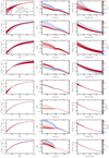 |
Fig. A.1. Dependence of the UVLF, 2PCF and galaxy bias at z = 6 on model parameters. Different rows show the UVLF (left), 2PCF (middle) an bias (right column) for different values of the seven model parameters σUV, ϵ0, log Mc, β, γ, log Mcut, log Msat, αsat. One parameter is varied at a time while keeping the others at their fiducial values (shown in the top right panel). |
Appendix B: Best-fit parameter values
Posterior median and 1 σ uncertainty of the model parameters.
Appendix C: Fits of the ultraviolet luminosity function
In Fig. C.1 we show the UVLF fits for each individual measurement.
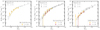 |
Fig. C.1. Fits of UVLF for each individual measurement, color coded accordingly. We plot the models only in the MUV range of the UVLF measurement. These show a good fit between the model and measurements in all z-bins. |
Appendix D: Details on the halo occupation distribution-model derivation of the correlation functions
D.1. Clustering correlation function
Described briefly, a central component of the model is the galaxy-galaxy power spectrum. It can be separated into contributions from the clustering of galaxies within the same halo (one-halo term) and from galaxies between different halos (two-halo term):
 (D.1)
(D.1)
These two components of the power spectrum of galaxies can be modeled under the HOD framework (Cooray & Sheth 2002; Berlind & Weinberg 2002) where the one-halo and two-halo terms are given by
![Mathematical equation: $$ \begin{aligned} \begin{aligned}&P_{\rm gg}^{1\mathrm h}(k,z) = \dfrac{1}{\bar{n}_g^2}\displaystyle \int \mathrm{d} M_h \dfrac{\mathrm{d} n}{\mathrm{d} M_h} \left[ \langle N_s \rangle ^2 u_s^2(k) + 2 \langle N_s \rangle \, u_s(k) \right], \\&P_{\rm gg}^{2\mathrm h}(k,z) = \\&\dfrac{1}{\bar{n}_g^2} \left[ \displaystyle \int \mathrm{d} M_h \dfrac{\mathrm{d} n}{\mathrm{d} M_h} b_h(M_h,z) \left[ \langle N_c \rangle + \langle N_s \rangle \, u_s(k) \right] \right]^2 P_{\rm lin}(k,z). \end{aligned} \end{aligned} $$](/articles/aa/full_html/2025/07/aa54618-25/aa54618-25-eq99.gif) (D.2)
(D.2)
In these equations,  is the mean number density of galaxies, bh(Mh, z) is the large-scale halo bias which we chose the one given by Tinker et al. (2010). us(k) is the Fourier transform of the over-density profile of satellite galaxies, for which we assume that it follows the NFW profile Navarro et al. (1997) with a mass-concentration relation as calibrated by Duffy et al. (2008). The important thing to note here is that the power spectrum is defined in terms of the occupation distributions of centrals and satellites ⟨Nc⟩ and ⟨Ns⟩ specified by Eq. 8 & 9 and is where the HOD parametrization enters the model. The linear power spectrum Plin(k, z) enters the two-halo term and dominates large scales. Details on deriving the spatial galaxy correlation function ξ(r) and the angular correlation function w(θ) using Limber (1953) equation are given in Blake et al. (2008).
All Tables
All Figures
|
Fig. 1. Spatial distribution of the three line-emitting samples (Hα and [O III] from FRESCO and Hα from CONGRESS) in the GOODS-North and GOODS-South footprints (left and middle panels) that we consider in this analysis. The right panel shows their redshift distribution. The density histogram gray background in the left and middle panels shows the footprint of the random catalogs. |
| In the text | |
|
Fig. 2. Angular 2PCF measured from the Hα CONGRESS and FRESCO samples at z ∼ 4.3 and z ∼ 5.4 and [O III] sample at z ∼ 7.3 selected at MUV < −19.1 mag. Comparison with literature measurements includes Harikane et al. (2022), Dalmasso et al. (2024a), and Paquereau et al. (2025) for samples selected at similar redshifts and MUV as our work. |
| In the text | |
|
Fig. 3. Best-fit models of the 2PCF and UVLF. Top row: Angular 2PCF measured from the Hα CONGRESS and FRESCO samples at z ∼ 4.3 and z ∼ 5.4 and [O III] sample at z ∼ 7.3 (orange points). Bottom row: UVLF for the same line emitter samples from Covelo-Paz et al. (2025), Meyer et al. (2024) along with the photometrically selected samples from Bouwens et al. (2021). The blue curves and envelopes show the median models and 1σ uncertainty computed from the posterior. In the case of the UVLF, for simplicity we show only the models in the same redshift bins as the 2PCF measurements. We show the individual fits for each measurement in Fig. C.1. |
| In the text | |
|
Fig. 4. Mean halo mass for the three line emitter samples: Hα samples at z ∼ 4.3 and 5.4 and [O III] at z ∼ 7.3 with MUV < −19.1 mag. We compare with measurements from Harikane et al. (2016) and Harikane et al. (2022) for photometrically selected LBG. The colored regions are derived from the EVS (Lovell et al. 2023) formalism and indicate the confidence intervals to observe the most massive halo in the GOODS volume (2 × 60 arcmin2) within the ΛCDM model. The dotted line marks the median of the EVS distribution of the maximum plausible halo mass. |
| In the text | |
|
Fig. 5. Galaxy bias as a function of redshift and MUV. The empty circles with error bars show the bias for the three line emitter samples Hα at z ∼ 4.3 and 5.4, and [O III] at z ∼ 7.3 with MUV < −19.1 mag. The solid blue lines show the bias as a function of redshift for four MUV thresholds computed from our model. We compare with measurements from Harikane et al. (2016), Dalmasso et al. (2024b) and Dalmasso et al. (2024a) for photometrically selected LBG, as well as Paquereau et al. (2025) for stellar mass selected, normal galaxies. |
| In the text | |
|
Fig. 6. Relationship of MUV − Mh (or UVHMR) for the redshift bins of our three line emitter samples. The solid lines and bold envelopes mark the MUV range that we probe with the 2PCF, while the transparent envelopes mark the range probed by the UVLF. We compare with the model by Mason et al. (2015, 2023) that includes dust attenuation in dashed lines and the observational measurements from Harikane et al. (2022) in dots. |
| In the text | |
|
Fig. 7. Star formation efficiency as a function of halo mass for the redshift bins of our three line emitter samples. The solid lines and bold envelopes mark the MUV range that we probe with the 2PCF, while the transparent envelopes mark the range probed by the UVLF. We compare with the observational measurements using 2PCF and HOD from Harikane et al. (2022) in dotted lines, empirical model by Tacchella et al. (2018) in dashed line, and results from cosmological simulations by Ceverino et al. (2024) and Feldmann et al. (2025) in solid colored lines. |
| In the text | |
|
Fig. 8. Resulting values of the model parameters. These values were obtained by drawing 1000 samples from the posterior and evaluating the models at a given z using Eq. (18). The orange points and errorbars mark the redshift bins of the 2PCF measurements. The dashed lines mark the z-parametrized functions (Eq. (18)) for our model parameters, evaluated at the median posterior. |
| In the text | |
|
Fig. 9. Scatter in the MUV−Mh relation, represented as σUV, as a function of redshift. The blue points with errorbars mark σUV at the median redshift of our three line emitter samples, while the blue line and envelope mark the best-fit and 1σ uncertainty as a linear function of redshift. From the literature compilation, the colored boxes at the right axis show the σUV for a range of Mh independent of redshift from the FIRE and FIREBOXHR simulations (Sun et al. 2023; Feldmann et al. 2025). For Muñoz et al. (2023), we show the 1σ contours for σUV obtained for independent z-bin fits; while the dashed purple line shows their best-fit linear function with redshift. For Ciesla et al. (2024) we show results from two different methods in the filled and empty squares. |
| In the text | |
|
Fig. 10. Predictions of UVLF out to z = 13 from our model constrained on z < 8 data and compared to measurements from the literature. The solid lines correspond to the model evaluated at different redshifts from the best-fit linear redshift dependence of the model parameters fit on 4 ≲ z ≲ 8 data. The dashed and dotted lines illustrate the two extreme scenarios of increasing SFE versus increasing stochasticity and show the model where we tune by hand ϵ0 and σUV to approximately match the observations, while keeping the other parameters nominal. The filled area shows the effect of dust attenuation on the UVLF, with the upper thin lines marking the unatenuated UVLF. |
| In the text | |
|
Fig. A.1. Dependence of the UVLF, 2PCF and galaxy bias at z = 6 on model parameters. Different rows show the UVLF (left), 2PCF (middle) an bias (right column) for different values of the seven model parameters σUV, ϵ0, log Mc, β, γ, log Mcut, log Msat, αsat. One parameter is varied at a time while keeping the others at their fiducial values (shown in the top right panel). |
| In the text | |
|
Fig. C.1. Fits of UVLF for each individual measurement, color coded accordingly. We plot the models only in the MUV range of the UVLF measurement. These show a good fit between the model and measurements in all z-bins. |
| In the text | |
Current usage metrics show cumulative count of Article Views (full-text article views including HTML views, PDF and ePub downloads, according to the available data) and Abstracts Views on Vision4Press platform.
Data correspond to usage on the plateform after 2015. The current usage metrics is available 48-96 hours after online publication and is updated daily on week days.
Initial download of the metrics may take a while.