| Issue |
A&A
Volume 699, July 2025
|
|
|---|---|---|
| Article Number | A59 | |
| Number of page(s) | 36 | |
| Section | Cosmology (including clusters of galaxies) | |
| DOI | https://doi.org/10.1051/0004-6361/202553903 | |
| Published online | 01 July 2025 | |
Explaining JWST star formation history at z∼17 by modifying ΛCDM
1
Main Astronomical Observatory of the National Academy of Sciences of Ukraine, 27 Akademik Zabolotny St., Kyiv, 03143, Ukraine
2
Astronomical Observatory, Taras Shevchenko National University of Kyiv, 3 Observatorna St., 04053 Kyiv, Ukraine
3
Department of Physics, University of Aberdeen, Aberdeen AB24 3UE, UK
⋆ Corresponding author: oleksii.sokoliuk@mao.kiev.ua
Received:
26
January
2025
Accepted:
22
April
2025
Recent cosmological observations indicate a 5σ discrepancy between the values of the Hubble constant H0 derived from late and early Universe probes, and a further possible tension at the ∼3σ level has arisen from different measurements of σ8. These measurements suggest the existence of new physics. In this work, we explore several theories of modified gravity that may help resolve these cosmological tensions. These include a family of phenomenological modified theories, where only Newton's gravitational constant and the Einstein-Boltzmann equations are affected. We considered one particular class of these theories: cosmologies with a varying growth index γ and a varying dark energy equation of state (EoS) wΛ. We also considered the normal branch of the Dvali-Gabadadze-Porrati (nDGP) model and k-mouflage gravity, which involves a non-trivially coupled scalar field. Our main aim is to narrow down the modified gravity landscape by constraining each model using high-redshift JWST data. Several probes are considered in this work: the stellar mass function (SMF), stellar mass density (SMD), star formation rate density (SFRD), and ultraviolet luminosity function (UVLF) along with the Epoch of Reionisation (EoR). The theories we considered are parameterised using rc (the scale length on which five-dimensional gravity transitions to four dimensions, for nDGP), β (associated with the Weyl re-scaling of the metric tensor), and K0 (quantifying aspects of the scalar field, for k-mouflage). The analysis carried out in this paper provides new constraints on these parameters. Generally, we find that the choice of rc≳103.5 Mpc is preferred for nDGP, while β∼0.1, K0≳0.9 is favoured for k-mouflage. Moreover, in the context of phenomenological gravity, phantom-like and ΛCDM cosmology with wΛ≲−1 is preferred over the quintessence.
Key words: galaxies: halos / galaxies: high-redshift / galaxies: star formation / galaxies: statistics / large-scale structure of Universe / dark ages, reionization, first stars
© The Authors 2025
 Open Access article, published by EDP Sciences, under the terms of the Creative Commons Attribution License (https://creativecommons.org/licenses/by/4.0), which permits unrestricted use, distribution, and reproduction in any medium, provided the original work is properly cited.
This article is published in open access under the Subscribe to Open model. Subscribe to A&A to support open access publication.
1. Introduction
Following the discovery of the late-time accelerated expansion of the Universe through the distance moduli of supernovae (Riess et al. 1998), the simple Λ cold dark matter (ΛCDM) theory was established as a standard cosmological model, as it both accurately explained the expansion of the Universe and matched most of the observations at the time. With recent technological advances, uncertainties in the data have been largely reduced, making it possible to obtain a constraint on cosmological parameters with a percent accuracy. Such a level of precision has revealed several discrepancies within the ΛCDM model. (For more details on that matter, see Perivolaropoulos & Skara 2022; Abdalla et al. 2022; Anchordoqui et al. 2021; Buchert et al. 2016; Di Valentino et al. 2021 and references therein.) There exist several cosmological tensions. Of particular concern are the values of the Hubble parameter H0 and cosmic variance σ8. These tensions indicate a significant deviation in the measured parameters of late and early Universe probes, such as supernova distance moduli, cosmic microwave background (CMB), and baryonic acoustic oscillations (BAOs). Specifically, a recent study has found that Planck and SH0ES measurements of H0 deviate at a greater than 5.9σ significance (Di Valentino 2021), suggesting the presence of new physics.
Another important tensionalt has risen from the context of Big-Bang Nucleosynthesis (BBN). The ΛCDM predicts a significantly lower lithium abundance than expected from BBN models (Fields 2011), with a tension of up to 4σ. Yet another diffuculty for the ΛCDM was found in the collision velocity of two galaxy clusters, jointly named ‘El Gordo’. The measured colliding velocity for the cluster appears to exceed the upper bound provided by the standard cosmological model (Asencio et al. 2021). Lastly, many other problems within the fiducial cosmology exhibit smaller tensions of the order of ∼3σ (Perivolaropoulos & Skara 2022).
There are other issues apart from cosmological tensions that challenge the ΛCDM. For instance, horizon and flatness problems require an extreme level of fine-tuning such that ρ/ρc∼10−53 at present, which can be provided by the inclusion of an inflationary phase around t∼10−35 s (Hu et al. 1994). Inflation is usually considered to be a part of the standard cosmological model, but it has several shortcomings. Firstly, it includes an extremely large set of solutions that fit the observational data, creating an ‘inflationary landscape’ (Marsh et al. 2013). Secondly, inflationary space-times have incomplete past geodesics, which hints at the existence of the initial singularity (Borde et al. 2003). Some theories beyond ΛCDM can address the fine-tuning without resorting to inflation or by solving the singularity problem (see Nojiri et al. 2017 for review). Other propositions to solve the flatness problem include the varying speed of light (Barrow & Magueijo 1999) and additional dimensions (Gen et al. 2002). Hence, at minimum, one needs to modify the early Universe physics within ΛCDM to match the observational data.
From the quantum perspective, Lagrangian density for ΛCDM is linear in the Ricci scalar, R, thus preventing it from being canonically quantisable (’t Hooft & Veltman 1974). Specifically, a Feynman diagram for a gravitational field interacting with a scalar field shows divergencies at a one-loop level. As a result, the ΛCDM lacks the required properties to be a viable theory of quantum gravity, which can pose a problem since it is expected that quantum gravitational effects dominate at t<tPl. Additionally, predictions for the value of the cosmological constant, derived from the quantum field theory and cosmological observations differ by up to 122 orders of magnitude, commonly referred to as the cosmological constant problem (see Weinberg 1989; Martin 2012 for further discussion).
As shown in Stelle (1977), the renormalisation issue can be resolved by adding higher-order terms, such as the contraction of a Riemann tensor, RμναβRμναβ, to the gravitational sector, making the theory renormalisable at the one-loop level. However, this approach suffers from the presence of Weyl ghosts. A model that avoids this issue is the R2 model, a promising candidate for a fiducial cosmology. It also serves as a viable model of cosmological inflation due to the presence of massive scalaron (Starobinsky 1980), but it remains UV incomplete.
Interestingly, modified gravity can also partially address most of the problems in classical cosmology. For instance, Saridakis et al. (2021) found that numerous models of modified gravity can alleviate both Hubble and σ8 tensions to an acceptable significance of ≲2σ. Moreover, theories such as the well-known f(R) one have successfully unified both the inflationary and late time accelerated expansion phases (Nojiri & Odintsov 2011, 2003). On the other hand, some special cases of the Gauss-Bonnet theory passed the Solar System and other tests on larger scales, addressed the hierarchy problem (Cognola et al. 2006), and the UV completion at the quantum level. Another interesting approach to go beyond ΛCDM is to construct theories based on various affine connections. For example, the choice of a Weitzenböck connection leads to the presence of the so-called torsion and the emergence of teleparallel gravitation (Bengochea & Ferraro 2009), which can mimic the behaviour of dark energy without actually introducing any other fields apart from the Standard Model (SM) Lagrangian. As noted in The FADE Collaboration (2022), some attempts have also been made to approach the cosmological constant problem with the help of modified gravity. However, we still lack the understanding of the nature of Λ in both the classical and quantum sense, and thus we cannot properly assess the reason behind the cosmological constant problem. These examples demonstrate that the use of modified gravity may be very effective in solving long-standing problems in modern cosmology and high-energy physics. Next, we discuss the specific models that have been chosen in the present work and the motivation behind our choice.
Phenomenological modifications to gravity represent the simplest way to minimally modify the ΛCDM model. Such modifications avoid any additional fields, and instead they only make slight alterations, such as setting a time-dependent cosmological constant or changing its EoS and adjusting the lensing equations. Interestingly, phenomenological theories can significantly impact the non-linear evolution of matter and, consequently, its power spectrum, which is a key focus of this work. However, these changes are only minor adjustments to the ΛCDM and thus allow us to preserve many of the successful features in the fiducial model, such as mass conservation and the preservation of the cosmological principle at scales greater than ∼100 Mpc. These features may be absent in theories that depart from ΛCDM significantly (e.g. those with different affine connections, new matter fields, or non-minimal interactions between sectors). The exact formalism for phenomenological modified gravity was first introduced in the pioneering works of Amendola et al. (2008), Zhang et al. (2007) and then rigorously tested with the CMB data by the Ade et al. (2016). Being phenomenological, these models lack a strong theoretical motivation. However, the functions representing the effective gravitational constant and gravitational slip were derived taking into account cosmological observations. Hence, as phenomenological gravity modifies solely the dark energy component, all of the affected quantities will revert to ΛCDM values as z→∞, similarly to other effective dark energy models. This ensures that the beneficial features of the ΛCDM in the early Universe are preserved.
Another and rather interesting minor modification of the ΛCDM is the wγCDM model. It affects the dark energy equation of state (EoS), allowing one to explore the behaviour of phantom and quintessence cosmologies by varying wΛ, and the evolution of matter overdensity via the growth index γ. This theory is also largely phenomenological. However, unlike the μ−Σ parameterisation discussed in Section 2, wγCDM generally does not respect the law of baryon conservation. The methodology regarding the implementation of varying γ in the cosmological background was first introduced in Pogosian et al. (2010) and later extended to wΛ≠−1 cases in Sakr & Martinelli (2022).
The normal branch of the Dvali-Gabadadze-Porrati (nDGP) theory is a widely used modified gravity model. It introduces an additional scalar field for a screening of gravity. This way, one can retrieve General Relativity (GR) at small scales and high overdensities. Key properties of nDGP gravity and effects of the braneworld formalism on different observable quantities in modern cosmology were discussed in the review paper Maartens & Koyama (2010). It is one of the few theories for which the full non-linear power spectrum was derived using the high-resolution N-body simulations (e.g., see Koyama 2016; Schmidt 2009). Baryonic effects on the power spectrum have also been quantified through the series of complex simulations of galaxy formation and evolution (Hernández-Aguayo et al. 2021). Studies have shown that some particular cases of nDGP pass Cosmic Microwave Background (CMB), supernovae distance ladder, and BAO, fσ8 tests (Lombriser et al. 2009; Zhao et al. 2016; Baker et al. 2019; Barreira et al. 2016). However, it is worth mentioning that this model still requires the presence of a small amount of dark energy to be viable, which may be considered a major flaw.
The final model of modified gravity that we consider is the class of k-mouflage theories. It is a generalisation of the k-essence cosmologies, and in a physical sense, it is close to Jordan-Brans-Dicke (JDB) theory of gravity, as both models use a non-canonical scalar field to drive the accelerated expansion of the Universe. Unlike JBD gravity, which is generally unscreened, k-mouflage always has a screening mechanism. However, this topic is still actively discussed, as JBD can be taken as a special limit of Horndeski scalar-tensor theory, which is prone to screening (Avilez & Skordis 2014). In a way, this mechanism is similar to nDGP, but the scales at which screening occurs are vastly different (Brax & Valageas 2014b). First introduced in Babichev et al. (2009), k-mouflage's cosmological properties at both linear and non-linear scales were explored in a series of works (Brax & Valageas 2014b, 2016, 2014a; Brax et al. 2015). These studies showed that in some cases, k-mouflage can rival the ΛCDM when given a constrained set of parameters and an appropriate form of the non-canonical scalar field potential K(χ), where χ is the scalar field. However, at smaller scales, such as within the Solar System, k-mouflage becomes highly non-linear and unstable due to the presence of higher-order modes in the field equation. This makes it challenging to decide on the validity of a theory on such scales (Brax & Valageas 2014c).
Apart from the problems already mentioned, another major obstacle is the modification of gravity itself. The CANTATA network (Saridakis et al. 2021) reports that there are tens, if not hundreds, of modified gravity theories that can provide viable cosmological evolution and potentially solve the Hubble tension. However, as mentioned in Ade et al. (2016), some of those ‘viable’ theories may arise due to a statistical bias in the data. The issue is that there are too many models, and an effective way of testing those models and distinguishing the few that are actually viable is yet to be found. One of the key aims of this work is to use JWST data to determine the viability of the models that we consider while hopefully narrowing the so-called modified gravity landscape.
Our manuscript is structured as follows: Section 1 presents the motivation for this study, a brief overview of the ΛCDM model and its modifications, and a literature survey of past studies on this topic. In Section 2, we introduce the basic formalism of modified gravity, including the background field equations, and first-order linear perturbations of the energy density, with modified values of effective gravitational constant and Bardeen potentials. We then introduce each modified gravity theory in greater detail within the same section and show the exact form of functions μ(a,k) and γ(a,k), which are implemented into the altered version of the CLASS1 code. Section 3 presents the derivation of a halo mass function (HMF) and the critical overdensity threshold δc for each theory. In Section 4, we present a similar formalism for the stellar mass function (SMF) and stellar mass density (SMD). In Section 5, we introduce the ultraviolet luminosity function (UVLF), while in Section 6, the Epoch of Reionisation (EoR) is introduced. Appendix A shows the observational data and theoretical predictions along with a detailed discussion on the constrained parameter space. Section 7 provides some concluding remarks. Figure 1 presents a step-by-step flow chart for each quantity of interest derived in this work.
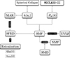 |
Fig. 1. Structure of this paper. |
2. A class of modified gravity theories
In this section, we introduce models of modified gravitation used throughout this paper and various cosmological observables that are related to the respective models. We adopted the Planck2018 TT,TE,EE+lowE+lensing+BAO cosmological parameters (Planck Collaboration VI 2020)


Ideally, a more detailed analysis would involve the application of each modified gravity model we consider to the Planck (or other) cosmological datasets in order to derive new parameters in each case. Other studies (L’Huillier et al. 2018; Ruiz-Zapatero et al. 2022) have considered the implications of this assumption, noting that there should be no significant alterations to the main conclusions.
We do not use the natural system of units GN=c=ℏ = 1. Rather, we work in the units of solar mass M⊙, which is required to derive observable quantities mentioned in the previous section. Also, the metric signature is taken to be mostly positive, that is, sigg=(−,+,+,+). Such a choice is purely a matter of preference, but it can also be motivated while working in both relativistic and non-relativistic quantum field theories.
2.1. Phenomenological modified gravity
The first model we consider is a phenomenological Modified Gravity (MG). Throughout this paper, we will not depart from the Friedmann–Lemaître–Robertson–Walker (FLRW) line element. We added a small scalar perturbation in a Newtonian conformal gauge:
![$$ {\mathrm {d}}s^2 = a^2(\tau )\bigg [-(1+2\Psi ){\mathrm {d}}\tau ^2+\sum _{i,j}(1-2\Phi )\delta _{ij}{\mathrm {d}}x^i{\mathrm {d}}x^j\bigg ], $$](/articles/aa/full_html/2025/07/aa53903-25/aa53903-25-eq5.gif)
where a(τ) is the scale factor. Ψ and Φ are Bardeen potentials, that depend both on conformal time τ and conformal coordinates x=(x1,x2,x3). To describe the matter content of the Universe, we adopted a perfect fluid energy-momentum tensor of the form

Here, we let μ,ν∈{0,…,3} be free indices; ρ, p represent the energy density and isotropic pressure of the perfect fluid respectively; and U=(1,0,0,0) denote the time-like four-vector. Next, we could perturb the perfect fluid energy-momentum tensor (Zucca et al. 2019):
Here, vi denotes the velocity field, while δT, δp are the perturbed parts of energy-momentum tensor and pressure respectively. Besides,  is the spatial part of anisotropic energy-momentum tensor, that is also traceless such that Tr π = 0. Additionally,
  represents the overdensity of the perfect fluid field. Since the energy-momentum conservation,
  , is the key feature of most cosmologies, one can derive a set of field equations based on it in the Fourier space (Bertschinger 2006):

Following the usual notation, we defined θ=div v. Parameter w is the matter EoS, that is taken to be a constant. Moreover, k is the wavenumber, typically measured in the units of Mpc−1. Finally,

is the conformal Hubble parameter. Equations (4) and (5) can be used to study any kind of decoupled fluid, such as cold dark matter (CDM), photon-baryons, or massive neutrinos. However, aforementioned equations still contain several unknowns, requiring two additional relations for potentials Φ and Ψ:
This equation is derived by combining the time-time and the divergence of the time-spatial components of the conservation Equation (3). An additional unknown is introduced while deriving the exact form of the potential Φ in Eq. (7). It is exactly the gauge invariant density contrast:
From the traceless part of the spatial-spatial component of the conservation equation, we derived the following equality:

Combining (9) and (7), we also obtained the parameterisation of Ψ in terms of Δ:

Equations (4), (5), and (9), (10) provide a closed system, governing the evolution of density contrast, velocity divergence, and both Bardeen potentials. These equations can be used as an input for Einstein-Boltzmann solvers CAMB (Lewis et al. 2000), and CLASS (Lesgourgues 2011), their numerous modifications. Here, we are primarily interested in the evolution of those quantities within the phenomenological modified gravity. So far, we have only used ΛCDM background cosmology. In certain modified gravity theories (for instance, family of scalar-tensor models), the relation between Ψ and Φ (9) is altered. This is effectively represented by an additional, “fifth” force between particles, which accelerates (or decelerates) the development of the large scale structure of the universe. These changes can be introduced by adding two functions of time τ and scale k into the evolution equations:
![$$ \begin {array}{l} k^2\Psi = - 4\pi G\mu (a,k) a^2[\rho \Delta + 3(\rho +p)\sigma ], \\ k^2(\Phi -\gamma (a,k)\Psi ) = 12\pi G\mu (a,k) a^2 (\rho +p)\sigma . \end {array} $$](/articles/aa/full_html/2025/07/aa53903-25/aa53903-25-eq18.gif)
The function μ(a,k) either reduces or enhances the gravitational force between particles (i.e. scales the gravitational constant GN). In a similar manner, γ(a,k) scales Bardeen potential Ψ. In the literature, γ(a,k) is often referred to as a gravitational slip function, and it is not directly related to any cosmological observable (Amendola et al. 2008, 2013). This makes it challenging to constrain such a function using present-day observational datasets, such as CMB, BAO, OHD, or Pantheon. The issue can be addressed by adopting a slightly different notion of phenomenological modified gravity (Zucca et al. 2019):
![$$ k^2(\Phi +\Psi ) = -4\pi G\Sigma (a,k) a^2[2\rho \Delta +3(\rho +p)\sigma ]. $$](/articles/aa/full_html/2025/07/aa53903-25/aa53903-25-eq19.gif)
The function Σ(a,k) relates the sum of Bardeen potentials to the gauge-invariant density contrast. In an absence of anisotropic stress, it is given by an equality Σ=μ(1+γ)/2. To derive the matter power spectrum and transfer functions, from the beginning of the epoch of reionisation (“cosmic dawn”) to the present time, we will use the MG-CLASS code (Sakr & Martinelli 2022), which adopts μ−Σ−γ parameterisation. Modified gravity background is turned on at z = 99, beyond that point, it is assumed that the background is represented by the ΛCDM. For phenomenological theories, ΛCDM background will be restored automatically anyway at high redshifts, but for the screened theories this is just an educated guess. If one will not make this assumption, we will have to change some parameters concerning BBN in MG-CLASS, which has not yet been properly constrained within our modified gravity context. At this stage, all we know about μ and Σ functions is that they are time and scale dependent. To perform numerical analysis, their exact forms must be properly specified. MG-CLASS implemented a couple of parameterisations. The first one we used is the Planck parameterisation (Zhao et al. 2009a):
Here, i∈{1,2} and fi represent the set of functions controlling the amplitude of scale deviations, and they depend on the dimensionless dark energy cosmological parameter and free parameter Eii:
As fi vanishes at early times, given that lima→0ΩΛ(a) = 0, the ΛCDM is recovered at sufficiently high redshifts. Following the pioneering work of Sakr & Martinelli (2022), we assume that functions μ and γ are independent of wavenumber, setting ci = 1. We consider all possible permutations of two sets, {1,−1,0}∈E11, {−1,…,1}∈E22 with |E22| = 10, resulting in 30 possible realisations of Planck parameterisation.
The second parameterisation, often referred to as “z_flex”, is independent of cosmological observables and always recovers GR at early times (Nesseris et al. 2017; Sakr & Martinelli 2022):
Here, gμ, gγ, and n are free parameters representing additional degrees of freedom to be constrained. To reduce the parameter space, we imposed the constraint n = 1.
The last kind of phenomenological modified gravity theory does not have any particular motivations from high energy physics or cosmology, but is still an interesting choice. This model relies on the Taylor expansion of μ(a) and is usually referred to as a Dark Energy Survey (DES) parameterisation (Sakr & Martinelli 2022):
Here, Ti, i={1,2,3,4} and n represent the set of free parameters to be constrained in the later sections. With five free parameters, the calculations become computationally expensive. To reduce the parameter space, we take n = 1, similarly to the z_flex case, and adopt T1=T3, T2=T4. In this way, we are left with only two free parameters. The parameter spaces for both z_flex and DES models are sampled similarly to the Planck parameterisation. Using the MG-CLASS code, we plot the matter power spectrum Pm(k) for each phenomenological modified gravity theory under our consideration. For comparison, we also show WMAP/ACT measurements (Tegmark & Zaldarriaga 2002) as well as observational data from Ly-α forest spectroscopy of distant quasars (Croft et al. 2002; Gnedin & Hamilton 2002). The resulting plots are located in Figure 2.
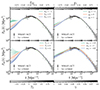 |
Fig. 2. Matter power spectrum predictions for phenomenological modified gravity versus observational data with varying values of E11, E22 (first subplot), gμ, and gγ, constant n = 1 (second subplot); for varying values of T1=T3 and T2=T4, constant n = 1 (third subplot); a running growth index γ; and dark energy EoS wΛ (fourth subplot). |
Having introduced all of the necessary quantities needed for the case of phenomenological modified gravity, we can proceed to review other models.
2.2. Varying γ and wΛ
In this case, we depart from the ΛCDM model by varying both the growth index of linear perturbations γ and dark energy EoS wΛ. We note that this γ is the scalar and has nothing to do with function γ(k,a) from Eqs. (13), (15) and (16). The growth index can be defined in terms of a growth rate as follows:
Here, D(a) = δ(a)/δ(1) represents the normalised growth of perturbations, obeying a second-order partial differential equation of the form:
![$$ \delta ^{{''}}(a) +\bigg [2+\frac {H^{{''}}(a)}{H(a)}\bigg ]\delta ^{{''}}(a) = -\frac {3}{2}\frac {\Omega _m(a)}{E(a)}\mu (a)\delta (a). $$](/articles/aa/full_html/2025/07/aa53903-25/aa53903-25-eq25.gif)
According to Sakr & Martinelli (2022), for this model, the evolution of both Bardeen potentials is governed by a system of equations:
By combining the system of equations above with the evolution equation for δ(a) from (18), the exact form of μ(a) can be derived (Sakr & Martinelli 2022):
![$$ \begin {array}{c} \mu (a) = \frac {2}{3}\Omega ^{\boldsymbol {\gamma }-1}_m(a)\bigg [\Omega ^{\boldsymbol {\gamma }}_m(a)+2-3\boldsymbol {\gamma }+3\bigg (\boldsymbol {\gamma }-\frac {1}{2}\bigg )\\ \times (\Omega _m(a)+(1+{{\mathit {w}}}_\Lambda )\Omega _\Lambda )\bigg ]. \end {array} $$](/articles/aa/full_html/2025/07/aa53903-25/aa53903-25-eq27.gif)
Plugging this function into MG-CLASS provides us with the accurate predictions for the matter power spectrum and CMB temperature angular power spectrum. In the ΛCDM limit, γ≈0.545 (Lightman & Schechter 1990; Lahav et al. 1991). We will take values of γ that deviate slightly around the ΛCDM prediction. For the dark energy EoS parameter, we probed both the phantom dark energy wΛ<−1 and quintessence −1<wΛ<0 cases. This specific model has been chosen due to the fact that as it appears, the most recent cosmological data have a preference for γ beyond ΛCDM (Specogna et al. 2024).
2.3. nDGP model
The widely known Dvali-Gabadadze-Porrati (DGP) model belongs to the large class of braneworld theories, where one assumes the existence of an n-dimensional brane embedded into a d dimensional bulk with d>n. Most braneworld models, such as Kaluza-Klein (Kaluza 1921; Klein 1926) or Randall-Sundrum (Randall & Sundrum 1999) take the simplest case, n = 4 and d = 5, which we are going to follow as well. The brane is represented by the usual FLRW geometry, while bulk space-time is Minkowski. The DGP model introduces a single additional free parameter, namely, a crossover scale rc measured in megaparsecs. The whole theory can be well defined by an Einstein-Hilbert action integral (Dvali et al. 2000):
In this action, M* is a five-dimensional Planck's constant, which determines the mass scale of the bulk dimension. Besides, y is the coordinate of the bulk dimension itself, and h=dethμν is the determinant of the 5d space-time metric hμν. Similarly, R and ℛ represent the Ricci scalar, based on the four and five dimensional manifolds respectively. Besides,  accounts for the cosmological constant that lives on a brane. For the sake of generality, the action defined above includes the contribution from a Lagrangian density ℒM[g,Γ,χi], which can contain various matter fields, both perfect fluid and not. Each arbitrary field is represented by
  (We note that in our case, as previously mentioned, we consider matter to be a perfect fluid). The relationship of those fields with gravity and space-time geometry is determined by g=det gμν and Γ (Levi-Cevita affine connection). The integration is performed over a four-dimensional Lorentzian manifold
  while dealing with the brane and over a five-dimensional manifold
  while working with the bulk. Under the least-action principle, it is straightforward to derive a modified Friedmann equation, governing the evolution of a DGP universe:
This study focuses on the nDGP model, which corresponds to ϵ=−1. Under the quasistatic approximation, commonly used by Einstein-Boltzmann solvers, the μ−γ parameterisation reduces to (Koyama & Maartens 2006)
The only unknown here is the Hubble parameter, which can be obtained using the modified Friedmann equation (22) and rewritten in a more familiar form:

where  with normalisation condition
  . The temporal derivative of the Hubble parameter is derived under the assumption that in nDGP, the conservation law for energy-momentum tensor is the same as in GR.
2.4. k-mouflage
The final model we consider, k-mouflage model, is based on k-essence, a model showing dynamical attractor behaviour. Similarly to the Jordan-Brans-Dicke case, it incorporates a scalar field but with an arbitrary kinetic term contribution (Babichev et al. 2009):
![$$ S=\int _{\cal {{M}}}d^4x\sqrt {-g}\bigg [\frac {M_p^2}{2}R+\mathscr {M}^4K(\chi )\bigg ]+S_{\mathrm {M}}. $$](/articles/aa/full_html/2025/07/aa53903-25/aa53903-25-eq38.gif)
Here, ℳ represents the scalar field energy scale, and K(χ) is the non-standard kinetic term, whereas χ is the rescaled scalar field
The action integral above is expressed in terms of the Jordan frame metric tensor gμν. Einstein and Jordan frames are related via the Weyl conformal transformation  . The field equations for the k-mouflage model are rather complex:
where
From Eq. (27), the Hubble parameter is derived in terms of the dimensionless mass densities for each matter and energy component, and a Hubble constant H0
The scalar field energy density is given by ρϕ=ℳ4/A4(2χK′−K). In k-mouflage models, mass densities follow the following relation: Ωm+Ωr+Ωϕ=(1−ϵ2)2. The model can be conveniently expressed as a set of functions that determine the deviation from ΛCDM (Benevento et al. 2019):
The only unknowns left are the choice of K(χ), A(ϕ), and ϕ. We note that MG-CLASS assumes the kinetic term is non-linear, while A(ϕ) is linear (Brax & Valageas 2014b; Sakr & Martinelli 2022):

Here, K0, and β are free parameters of the model, with m = 2, making K(χ) of quadratic order. We note that for k-mouflage, β has a different meaning in relation to the nDGP case, namely it controls the Weyl rescaling of the metric, which can be observed after expanding A in  . Plugging Eq. (31) into Eq. (28), we can simplify those quantities as follows:
Thus, the rescaled scalar field is  . The value of the scalar field at present is determined using the continuity equation:

From Equation (32), at the present time, ϵ2,0 = 0, giving Ωϕ0 = 1−Ωr0−Ωm0, which is very similar to the ΛCDM case. We can also fix the mass scale by manipulating the definition of the scalar field. However, in that case one needs make use of a set of initial conditions, and following the work Brax & Valageas (2014b), we adopt ϕ(1) = 0, from which it follows that
Equating this to (33) allows us to solve for ℳ4:
Finally, the exact form of the scalar field ϕ should be specified. It is calculated from the Klein-Gordon equation (Brax & Valageas 2016):
![$$ \frac {{\mathrm {d}}}{{\mathrm {d}}t}\bigg [A^{-2}a^3\frac {{\mathrm {d}}\phi }{{\mathrm {d}}t}K^{\prime}\bigg ]=-a^3\rho _m\frac {{\mathrm {d}}\ln A}{{\mathrm {d}}\phi }. $$](/articles/aa/full_html/2025/07/aa53903-25/aa53903-25-eq52.gif)
The resulting power spectra for screened theories is shown in Figure 3. We have defined each modified gravity theory that is of special interest to us in the current work. Now, we can proceed and derive some observables, such as halo mass function with the use of MG-CLASS. Similarly to the phenomenological theories of gravitation, for our future analysis we consider a range log10rc∈[2.5,4] (10 steps) and β∈[0.1,0.5] (3 steps), K0∈[0,1] (10 steps).
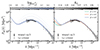 |
Fig. 3. Same as Figure 2 but for the nDGP gravity with varying rc (first subplot) and k-mouflage gravity with varying β, K0 (second subplot). |
3. Extracting HMF from linear matter power spectra
To constrain models beyond ΛCDM, we first need to obtain the Halo Mass Function (HMF). This cosmological observable can be derived using the extended Press-Schechter (EPS) approach introduced in the pioneering work of (Press & Schechter 1974):
Here,  is the halo mass, R is its corresponding radius. Besides,
  is the background density, and σ(R) is the variance of a density field, ν=δc/σ(R). We take c≈3.3, which seems to reasonably well approximate the HMF even beyond the ΛCDM (Parimbelli et al. 2021). For the ΛCDM cosmology, the linear density threshold is δc(z) = 1.686/D(z). We assumed for first-crossing distribution to have a Sheth-Tormen form (Sheth & Tormen 1999):
Here, A = 0.3222 and p = 0.3 are dimensionless constants that were derived from the best-fits to the simulation data. The variance of matter fluctuations is calculated as follows:
We defined Pl(k,z) as the linear matter-power spectrum, while WF(k,R) is the so-called window function

Recent results have shown that the value β = 4.8 provides a good fit to the data, extracted from N-body simulations (Leo et al. 2018). As mentioned earlier, the result δc(z) = 1.686/D(z) applies only to a ΛCDM model and will vary for its modifications (e.g., see Schmidt et al. 2010; Lombriser et al. 2013 as an example). To derive the value of a density contrast for modified ΛCDM, we need to explore the physics of spherical collapse.
3.1. Modelling spherical collapse
Under the spherical collapse formalism, the top-hat distribution is often assumed for simplicity, which is defined in the following way:
This indicates that the sphere of some radius R is filled homogeneously, having the density ρc>0. Since the density is non-zero, after some time, the sphere should eventually collapse due to its own gravitational pull in the absence of pressure, as we are considering matter to be dust-like. However, after the collapse, Birkhoff's theorem may no longer apply within modified gravity theory. As a result, Equation (41) will not hold, and thus some non-vanishing density contrast can appear outside of R (see Moffat & Toth 2009 for the implications of that violation). The applicability of this theorem will be discussed separately for each model in the next several sections.
To derive the value of the critical overdensity, we first introduce the set of non-linear continuity and Euler equations in real space. The first (continuity) equation, follows from the fact that the covariant gradient of the stress-energy tensor vanishes:

Here,  is the Christoffel symbol of the second kind:
Assuming that ν = 0, we can derive the continuity equation in the non-linear regime:
Inside and outside of the spherical region, we have different expansion rates and therefore different scale factors:

with  being the local Hubble parameter within the sphere and r as the local scale factor, respectively. Now, it is possible to define the non-linear overdensity as

Following the work of Abramo et al. (2007), we applied the first-order temporal derivative to the equation above:
For a pressureless fluid (such that p=pc = 0, i.e. dust), Eqs. (46) and (49) reduce to
Taking the temporal derivative of the relation above again, we get the equation that governs the evolution of the fluid in the non-linear regime within the FLRW universe
We recall that the second Friedmann equations inside and outside of a sphere are
From this, we deduced that
Substituting these expressions into Eq. (49), we obtained the final equation for the growth of δnl:
Here, we transform the gravitational constant G→Gμ(a). This deviation arises due to the modification of gravity. Since solving for cosmic time is challenging, we instead express the above equation in the terms of the scale factor. For that we use a change of variables  ,
,  , and
, and  . This works within ΛCDM and modified ΛCDM theories with no non-minimal couplings between different sectors. Thus, we have
The linear regime overdensity can be derived by combining Equations (4) and (5), as shown in Esposito-Farèse & Polarski (2001):

By applying the same transformation as for Eq. (53), this can be expressed in the terms of the scale factor (Tsujikawa 2007; Nesseris & Sapone 2015; Arjona et al. 2019)
Thus, linear overdensity evolution is recovered in Equation (53) if all contributions from  terms are ignored. To determine the exact value of the critical overdensity, we first find the scale factor ac at which δnl diverges (i.e. spherical collapse occurs), and then solve Eq. (55) such that δl(ac) = δc. Initial conditions for the non-linear differential equation (53) are assumed to match with the Einstein-de Sitter (EdS) case, since at an initial scale factor ai = 10−5, matter dominates (Ωm(ai)∼1) and modified gravity does not play a significant role. Consequently, at ai, the density perturbation takes the form
  (Malekjani et al. 2015, 2017) and
Those initial conditions are expected to lead to the collapse at the point when δnl(ac)≃107. Hence, we need to derive the value of δnl(ai), to ensure that at the desired scale factor, δnl(ac)≃107. This can be achieved by adopting the algorithm presented in Pace et al. (2017).
Since the matter field shows a linear behaviour at a≪1, initial conditions from Eq. (56) apply for both non-linear and linear cases. We show the linear density threshold for each phenomenological modified gravity in Figure 4.
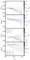 |
Fig. 4. Linear density contrast for the spherical collapse occurring at the time ac within DES, z_flex, and Taylor expanded DES, varying wΛ and γ phenomenological theories of gravitation. |
As can be seen, the nDGP and k-mouflage models are not included in the plots. This is because both of those theories involve the use of Vainshtein screening, which suppresses the so-called “fifth” force at small scales, where GR should be recovered due to the Cosmological Principle. The derivation of Eq. (53) for screened models is different, and the methodology for that will be discussed in the next subsection.
3.2. δc and screening of gravity
As it was previously mentioned, the process of obtaining δc within the nDGP gravity differs from the phenomenological theories due to the unique nature of this theory. On subhorizon scales, it was shown that matter within nDGP gravity follows the evolution equation (Schmidt et al. 2010):
Bardeen's potential here deviates from the GR prescription by the so-called “brane-bending mode”, a scalar field φ:
The Newtonian potential obeys the standard Poisson equation, while the brane-bending mode is described by Koyama & Silva (2007)
In Schmidt et al. (2010), the full profile of the brane-bending mode was calculated, and it was demonstrated that the ∇2φ is constant within the top-hat interior, similarly to the Newtonian potential ΨN. However, ∇2φ retains a non-trivial dependence on the energy density perturbation (Schmidt et al. 2010):

Here ΔGeff represents the difference between the modified gravitational constant and Newton's original gravitational constant. Additionally,
and the characteristic radii for nDGP and k-mouflage theories are represented in the following way (Brax & Valageas 2014a):
These two expressions represent the Vainshtein radius, a characteristic scale for nDGP and k-mouflage respectively, at which the screening takes effect. Further, we are not going to differentiate  and
and  , so that the value of Vainshtein radius R★ will depend on the theory that we are investigating. By combining Poisson's equations for scalar field and Newtonian potential, and using Eq. (57), we get the evolution equation for non-linear overdensity in terms of the scale factor:
This closely resembles Eq. (53). However, in the case when gravity is screened, the effective gravitational constant not only depends on the scale factor but also on the screening radius. The condition R≫R★ implies the fact that Geff/GN = 1+1/3β holds for nDGP, as noted in the previous subsection. Thus, in the case when the actual radius significantly exceeds the Vainshtein radius, the effects of screening can be ignored, and the equations from the previous subsection can be used to derive δc. However, if one assumes that δρ/ρ≫1, then Geff/GN∝(R/R★)3/2 (Schmidt et al. 2010). Linearising gravity substantially simplifies the calculations, and as shown in the paper Schmidt (2009), the matter power spectrum for both full and linearised nDGP is approximately the same. Besides, at high enough redshift z≫0, linearised and full nDGP gravity coincide, since R/R★→∞. But for consistency, we are going to keep the full nDGP physics and linearise it only for δl calculations. Our results for δc may differ from the work of Schmidt et al. (2010), as we do not adjust the effective dark energy EoS in the nDGP case, because H(a) would then correspond exactly to the ΛCDM prediction. Instead, we prefer to use the framework of Eq. (24).
Similarly to the nDGP scenario, Vainshtein-like screening also occurs within the k-mouflage cosmology, as mentioned in Brax & Valageas (2014b). In this work, we use the fact that at small enough scales, as in ΛCDM, each spherically collapsing sphere can be treated separately. This approach was first noted by the Lemaitre and its detailed version for k-mouflage theory was presented in Brax & Valageas (2014a). Thus, at the scales ctk/a≫1, our approximation works well. These scales exceed those of typical galaxy clusters, and therefore one could compute such quantities as halo mass function under the assumption that the screening is absent. On the other hand, the derivation for δnl gets complex beyond these scales, as screening should be taken into account as well. Numerical solutions for δl(a) in the screened gravity context are subsequently shown in Figure 5.
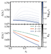 |
Fig. 5. Linear density contrast for the spherical collapse occurring at the time ac within screened MOG models, namely nDGP and k-mouflage. |
With derivation of dn/dlog Mh from the Eq. (37), we can now finally determine the observationally constrainable quantities, as outlined in the next subsection.
4. Stellar mass function and density estimates
The halo mass function (HMF) cannot yet be constrained by observational data directly; instead, existing constraints are only being derived using cosmological simulations. One cannot state the robust conclusions on the validity of a theory using the cosmological simulations alone. However, several quantities can be derived from the HMF, that in turn are constrained by the observational data. These are the stellar mass function (SMF) and the corresponding stellar mass density (SMD). In this study, we are particularly interested in JWST observations of galaxies across the redshift range z∼0−17. To obtain SMF and SMD, we apply an analytical approach, similar to the one used in Dayal & Giri (2023). In this approach, we first assume that each halo of mass Mh contains mass according to the relation Mg=(Ωb/Ωm)Mh. Some portion of baryonic mass within the halo converts to stars via star formation processes such that M★=ϵ★Mg. Here, ϵ★ is the star formation efficiency (SFE), which varies from one model of star formation to another. Typically, the value of star formation efficiency ϵ★ ranges from 2%, up to 100% in the extreme cases, as discussed in a greater detail by Kim et al. (2021). Most theoretical studies at high redshifts z∼5−10 assume that ϵ★ = 0.1−0.3 (Hirano & Yoshida 2023; Adil et al. 2023; Glazebrook et al. 2023).
In our case, we can follow the paper Dayal & Giri (2023), where they assumed two models of star formation, but it appears that their motivation for the first model is vague, and thus it is more appropriate to assume a more complex fit for ϵ★, derived from the computationally expensive cosmological simulations or the observational data. For the latter, we have chosen to use an approximation, derived from several deep sky surveys in the redshift range z∼0−8, as presented in the Behroozi et al. (2013), Rodríguez-Puebla et al. (2017).
Model I: In the Rodriguez-Puebla et al. approximation for ϵ★, the authors introduced a parametrisation of stellar mass to halo relation that gives a median stellar mass for each halo mass bin based on the formalism laid out in Behroozi et al. (2013), namely,
with
with x=log10(Mh/M1). Unlike the Behroozi et al. (2013) case, this parameterisation takes into account more accurate predictions for scatter in the SMHR, that are closer to the observational data at lower redshifts (see Mendel et al. (2014)). According to (Rodríguez-Puebla et al. 2017), best-fit functions have the following form:
Here, ν(z) = exp(−4/(1+z)2) and  (Rodríguez-Puebla et al. 2017). We account for observational systematics and various biases in SMHR by adopting the formulation (Behroozi et al. 2013):
Clearly, measured and true stellar masses deviate by a factor 10μ. The purpose of this offset is to account for possible uncertainties in the Initial Mass Function (IMF), the stellar population synthesis model, star formation history model, and redshift uncertainties for each galaxy in the sample. An additional parameter κ has to be introduced into relation (67) to account for the mass-dependent evolution of active galaxies. Further details on these parameters and their best-fit values can be found in Behroozi et al. (2013). For the fraction of passive galaxies, one can consider the formula given in Brammer et al. (2011).
Model II: Another way to parameterise the stellar mass to halo relation (SMHR) is to use the well-known and fairly straightforward double power-law best fit introduced in the pioneering work of Moster et al. (2010), Mirocha et al. (2017):
Here, ϵ★,0 represents the star formation efficiency at the peak mass Mh,0, while γlo and γhi are power-law indices. The values of these indices either suppress or enhance the star formation rate at low and high halo masses. Based on Mirocha et al. (2017) and the subsequent paper Shen et al. (2024), we take the following values that fit the observational data up to redshifts of z∼12: log10(Mh,0/M⊙) = 12, γlo=−0.6 and γhi = 0.5. We assume a fiducial value of ϵ★,0, specifically ϵ★,0 = 0.21. The double power-law function above is redshift independent, though the recent data in Conroy & Wechsler (2009) and other studies suggests that redshift dependence in SMHR should be present for the accurate representation of the observational data. The redshift-dependent baryon conversion ratio can be easily implement, following Mirocha et al. (2017):
The amplitude of star formation efficiency is fixed, but the peak halo mass can vary with redshift as follows:
The indices introduced above vary in the range −1≤γ★/M≤1. A redshift-independent SMHR is recovered when γ★=γM = 0.
Model III: This is an extreme case using ϵ★ = 1. This choice of constant baryon conversion ratio is likely not viable, since there is substantial evidence from the JWST CEERS survey that ϵ★ should vary with redshift, particularly in the range z∼4−8 (Chworowsky et al. 2023). Moreover, the 100% conversion is not realistic and contradicts the observational data previously mentioned. Thus, this case will only be used for illustrative purposes.
In this work, we assume that the least massive halos are of mass Mh,cut = 106.5 M⊙, which sets the cut-off scale of the stellar mass via the SFE relation. We now can define the stellar mass function itself in terms of the halo mass function. However, while deriving the HMF we did not account for many baryonic effects that arise, for example, AGN feedback, supernova feedback, nucleosynthesis (see how those effects contribute to star formation and IMF in the analysis of EAGLE Furlong et al. 2015, and STARFORGE Guszejnov et al. 2022 simulations). For a detailed explanation on how to include those effects into analytical models, refer to Salcido et al. (2020). Our double power-law SMHR already accounts for both stellar and AGN feedback, as mentioned in Moster et al. (2010). Stellar feedback strength is encoded into the parameter γlo, while AGN is encoded into γhi. On the contrary, since the Behroozi et al. approach relies solely on observational data for best fits, i.e. is practically model-independent, it also implicitly accounts for any baryonic physics present.
4.1. Stellar mass function
We derive the stellar mass function using the methodology of Boettner et al. (2025), which gives the following definition for the SMF:
Here we have used the halo abundance matching method, explained in Boettner et al. (2025). The equation above would work in an ideal scenario where no scatter is present in the SMHR relation. However, observational data, especially at higher redshifts, have significant uncertainties in M★, and hence scatter. The implementation of scatter into the SMF can be done using the formula provided in Behroozi et al. (2010):
In this equation, P(ΔM★) represents a log-normal Gaussian kernel of width σsf. Its value is redshift-dependent and defined in Rodríguez-Puebla et al. (2017). In addition to accounting for scatter in the observational data, we must get rid of statistical biases that may be present in the measurements of stellar mass (Behroozi et al. 2013) and the fraction of passive galaxies. We will not delve into details on the matter of derivation of fpassive,obs(M★,z), and instead refer to the Appendix C of Behroozi et al. (2013). We can now introduce the measured SMF as follows:
The observed SMF is the measured one multiplied by an appropriate factor c(z), namely the stellar mass completeness function
Incompleteness in the measurements of stellar masses arises mainly in the high-redshift surveys due to the non-ideal target selection criteria and many other factors. Recent studies have demonstrated that the stellar mass function completeness in CMASS BOSS (Leauthaud et al. 2016), DESI (Yuan et al. 2023) and COSMOS (Weaver et al. 2023) surveys can be modelled through the exponential fit with two degrees of freedom, amplitude A and onset redshift zc (Behroozi et al. 2013):
The statistical bias corrections κ, μ and constants A, zc, are provided in Behroozi et al. (2013).
We note that scatter corrections are only applied to the first two models described above, i.e. that associated with Rodríguez-Puebla et al. (2017) (Eqs. (64)–(67)) and the double power-law SMHR models (Eq. (68)). Model III, representing the extreme case with 100% SFE, is not directly connected to any observational data, and hence there is no scatter present. Additionally, we do not apply the survey completeness correction (75) to the double power-law SMHR, as it is calibrated on the observational UVLF data, which incorporates those corrections ab initio.
4.2. Stellar mass density
Finally, we define another quantity of special interest: cumulative halo mass density, which can be derived using the following equation (Boylan-Kolchin 2023):
Here, n(Mh,z) represents the number density of halos of mass Mh per unit volume. It is not possible to integrate up to infinity, as the HMF is a numerical rather than analytical quantity. Hence, we adopt an upper limit of an integral Mh,max = 1018 M⊙. Eq. (76) relates to the total mass concentrated in a halo. On the other hand, the cumulative stellar mass density only accounts for a stellar mass within a halo:

Here, we define f★=ϵ★(Ωb/Ωm). We note that even for our modified cosmologies, the fraction Ωb/Ωc is assumed to be constant throughout the redshift range we consider, because both Ωb∝a−3 and Ωc∝a−3. This assumption will not hold if one supposes some non-standard interactions between dark and baryonic sectors, causing the loss of baryons through cosmic time. With this, we can now proceed to derive another probe.
5. Ultraviolet luminosity function
Another useful observable which can be utilised is the UVLF. To derive the UVLF from the HMF, we use the relation similar to the one used for the stellar mass function, namely,
Here, MUV represents the dust-attenuated magnitude in the UV range. In order to fully specify MUV, several things must be done. We began by mapping between the star formation rate (SFR), characterised by the value of  , and the UV galaxy luminosity, LUV:
Typically, SFR is expressed in units of M⊙ yr−1, and UV luminosity in units of erg s−1 Hz−1. We note that some previous studies retain the dependence on h, reduced Hubble constant. This has been avoided in the present paper. In Equation (79), κUV = 1.15×10⁻²⁸ is the conversion constant, introduced in the review article by Madau & Dickinson (2014). This conversion factor is derived from the well-known Salpenter IMF (Salpeter 1955), and uses a UV wavelength of 1500 Å. For details on how the value of κUV changes with redshift, pivot wavelength λUV, metallicity Z/Z⊙ and IMF, refer to Boissier et al. (2013), Inayoshi et al. (2022), Madau & Dickinson (2014). Since the star formation rate is obtained from the dark matter halo mass, we need to calculate the halo Mass Accretion Rate (MAR)  first.
5.1. Mass accretion history
The  is typically derived from cosmological simulations (e.g. see Zhao et al. (2009b), Dhoke & Paranjape (2021) for cold and warm dark matter cosmologies, respectively). However, we can also achieve that analytically using the approximation derived from the aforementioned simulations by averaging over merger trees (van den Bosch et al. 2014), or from statistical data (McBride et al. 2009). In the current study, we assume the prescription for MAR derived in Neistein et al. (2006), which uses the familiar extended Press-Schechter formalism:
In Eq. (80), σq=σ(Mh(z)/q), where q is a free parameter that ranges from 2 to some qmax. The choice of qmax depends on the cosmological model adopted, but q is a free parameter, that varies within the given bound and can be derived using data from cosmological simulations. The approach taken in the present paper is to adopt the analytic expression given by Correa et al. (2015a):
The Eq. (80) can then be transformed into a mass accretion history (MAH) of the form
by integrating while also noting the fact that
![$$ \begin {array}{l} \beta = -f(M_0), \\ \alpha = \bigg [\delta _c \sqrt {\frac {2}{\pi }}\frac {dD}{dz}\bigg |_{z = 0}+1\bigg ]f(M_0). \end {array} $$](/articles/aa/full_html/2025/07/aa53903-25/aa53903-25-eq114.gif)
Here, M0 is the halo mass at present epoch, and the function  (Correa et al. 2015a). The form (82) is motivated by the study Wechsler et al. (2002). This study suggests that CDM halos behave as M(z)∼eβz at high redshifts, and as M(z)∼(1+z)α at lower redshifts. This transition arises due to the development of matter density, that is slowed down at late times, when dark energy component dominates. The MAR is obtained from Eq. (82) by differentiating with respect to redshift, and multiplying the resulting expression with dz/dt=−(1+z)H(z). This leads to (Correa et al. 2015a):
![$$ \begin {array}{c} {\dot {M}}_h(z) = 71.6\mathrm {M}_\odot \mathrm {yr}^{-1}\bigg (\frac {M(z)}{10^{12}M_\odot }\bigg )\bigg (\frac {h}{0.7}\bigg )\\ \times [-\alpha -\beta (1+z)]E(z). \end {array} $$](/articles/aa/full_html/2025/07/aa53903-25/aa53903-25-eq116.gif)
Subsequent work (Correa et al. 2015b) indicates that taking the mean 〈α〉 = 0.24 and 〈β〉=−0.75 works well over the halo mass range 108≤Mh≤1014 in the context of standard LCDM. Nevertheless, some theories exhibit sufficient deviations in Pm(k) from the ΛCDM theory, which in turn will lead to the deviation in 〈α〉 and 〈β〉 values, as power spectrum is directly incorporated into the value of f(M0). To address this issue, we compute these parameters explicitly with Eq. (83), taking δc from Section 3 and D(a) from Section 2. Parameters are defined over a discrete grid of halo masses 106.5≤Mh[M⊙]≤1018 and then linearly interpolated. This way, there are no inconsistencies, even when the departure from ΛCDM is significant.
Given the relationship in Eq. 79, we can now derive the UV luminosity. But the derived luminosity does not take into account various effects which can affect it on the way to the telescope detector. Those effects, and how they can be taken into account when calculating UVLF are discussed in the next subsection.
5.2. Dust attenuation and other effects in ultraviolet luminosity functions
From (79), we compute the intrinsic UVLF by integrating the following expression (Mirocha et al. 2021):
However, this expression does not account for an absolute UV magnitude, namely MUV. This is important, as most observations of the UVLF are expressed in terms of it. To relate the UV luminosity to its absolute magnitude, we factor in dust attenuation, which affects UVLF significantly at MUV≲−20 (see Shen et al. 2023 for comparison of intrinsic and corrected UVLF). Effects of dust are included with the well-known IR excess LIR/LUV (IRX)-β relation (Meurer et al. 1999)

Here, β is the UV spectral slope. Consequently, β can be related to the absolute magnitude MUV as follows (Cullen et al. 2023):

This expression was calibrated using JWST data to work within the redshift range z∼4−16. Finally, we account for the scatter arising from variation in the HMF (if one uses Sheth-Tormen (Sheth & Tormen 1999), Tinker (Tinker et al. 2008), or any other kind of HMF approach), AGN/stellar feedback models, and IMF assumptions. Scatter is modelled by smoothing the UVLF with a Gaussian kernel of width σUV. For clarification and methods, see the study by Shen et al. (2023). As noted in Duncan et al. (2014), Song et al. (2016), at higher redshifts (z≥8), σUV∼0.4 dex, down from σUV∼0.5−0.6 dex at z≤4. Additional scatter is observed due to the uncertainty in the stellar mass estimates, as the UVLF is connected to the star formation rate via Eq. (79). Shen et al. (2023) estimate that σUV∼2.5 dex in total at z∼16 and higher redshifts. In this work, we take σUV to be both mass and redshift dependent, following Gelli et al. (2024), Shen et al. (2024):
![$$ \sigma _{\mathrm {UV}}(M_{\mathrm {halo}}) = \max [{\cal {{A}}}-{\cal {{B}}}(\log _{10}(M_{\mathrm {halo}}/M_\odot )-10)+{\cal {{C}}},\sigma _{\mathrm {min}}]. $$](/articles/aa/full_html/2025/07/aa53903-25/aa53903-25-eq120.gif)
In Eq. (88), we use  , ℬ = 0.34 and σmin = 0.2 dex. We also set
  to be redshift-dependent, linearly interpolated from
  ,
,  ,
,  (Shen et al. 2024). Those parameters were derived on the basis of ΛCDM cosmology. Clearly, this is an approximation, as we are dealing with non-standard cosmology in this paper, but there are no estimates of σUV for our models yet available in the literature.
To calculate the UVLFs numerically, we have made use of the code highz-empirical-variability2, documented and firstly used in the paper Shen et al. (2023). The code was properly modified to accommodate for the modified theories of gravity.
5.3. Star formation rate density
We also need to calculate the Star Formation Rate Density (SFRD). It is defined in a similar way to the stellar mass density. The only difference is that we change mass inside the integral (76) to be the corresponding mass accretion rate. This leads to the following definition of the SFRD:
The SFRD will be used jointly with other quantities to obtain constraints from JWST in the next sections.
6. Epoch of Reionisation
The Epoch of Recombination, which occurred at z∼1100, converted most of the free electrons and protons into neutral hydrogen and helium. After this epoch, with few sources of ionising radiation, the Dark Ages lasted until z∼30, when the formation of first stars and galaxies brought it to an end. Radiation from the first luminous objects ionised neutral atoms, initiating the rise of the Epoch of Reionisation (EoR). However, the process of reionisation was not homogeneous - clouds of ionised gas were first formed at around z∼12 in massive galaxy clusters, in which there are embedded powerful sources of ionising radiation. Voids were ionised later, at z∼6 due to the gradual increase of an ambient UV radiation.
There are several physical quantities which can be derived during the EoR, but we focus on the ionised hydrogen fraction xHII and optical depth τreion. We are not concerned here with the reionisation of helium, which occurs much later. A parameter of particular interest, QHII, measures the volume filling fraction of H II. The end of reionisation epoch is reached as QHII∼1. We note that the time evolution of QHII is governed by the equation below (Wyithe & Loeb 2003; Madau et al. 1999):
Here, fesc represents the fraction of ionised photons that escape galaxies and reach the intergalactic medium (IGM). Some galaxies are very dusty, and thus the escape fraction for such objects should be very small, as most photons will be absorbed. In order to correctly reproduce predictions for xHII, we need to account for both the populations of dusty and unobscured galaxies. A paper that explores this topic further is Fudamoto et al. (2021). We take the value assumed by the SIMBA hydrodynamical simulation suite, namely fesc = 0.25 (Hassan et al. 2022). The exact values of the escape fraction vary in the literature, but generally lie in the range fesc∈[0.1,0.3]. Additionally, there is some evidence present for fesc evolving with redshift (Kuhlen & Faucher-Giguère 2012; Price et al. 2016).
Another unknown in Eq. (90) is the mean number density of all hydrogen species at z = 0, denoted by  . CHII is the clumping factor of H II. We take it to be CHII = 3.0 following Kaurov & Gnedin (2015). This value has been derived using a series of cosmological simulations, avoiding a redshift dependence, since the data are too uncertain to determine that reliably.
Besides, αB represents the case-B recombination coefficient, which sums over only excited states, i.e. all states excluding the ground one. case-A recombination sums over all hydrogen states. We can mention that the choice of case-B is appropriate, since the ionised hydrogen that is produced by the recombined neutral hydrogen in the ground state is usually absorbed by nearby thick clouds of gas, and hence does not reach the observer. This is also supported by the fact that at higher redshifts, an intergalactic medium can be considered to be highly opaque (Dijkstra et al. 2007). The recombination coefficient mainly depends on the temperature of ionised hydrogen, namely THII. Following the work Gong et al. (2023), it is fitting to assume THII = 2×10⁴ K (Robertson et al. 2015), resulting in a recombination coefficient αB = 2.5×10⁻¹³ cm3 s−1. For a detailed discussion on the choice of recombination coefficient, refer to Nebrin (2023) and references therein.
The only undefined quantity left in Eq. (90) is the production rate of ionising photons, which is usually calculated from (Gong et al. 2023; Mirocha et al. 2021)
The value of Nion, standing for the total flux of Lyman-continuum photons per solar mass per second, is usually derived from a Stellar Population Synthesis code (some of the widely used options include STARBURST99 Leitherer et al. (1999), or alternatively, BPASS Eldridge et al. (2017)) or from the observational data. Additionally, sophisticated and computationally expensive hydrodynamical simulations of structure formation can also be used for that purpose. For instance, in one of the recent works, THESAN-HR simulations (Shen et al. 2024b) have been used to explore the degeneracy of Nion between CDM and WDM/FDM/sDAO models. In this paper, following the prescription of Robertson et al. (2013, 2015), we adopt the value of Nion, derived from the Hubble Ultra Deep Field (HUDF) data such that log10Nion≈53.14.
An expression for QHII is given next. This equation must be evaluated numerically due to the complicated nature of Hubble parameter and ionising photon production rate. In Eq. (90), xe represents the abundance of electrons and is determined by xe=ne/(nH+nHe), assuming an absence of metals. Here, ne is the corresponding free electron number density. It is difficult to calculate the value of ne without making assumptions regarding the ionisation of other elements. For simplicity we assume that during the period of 20≥z≥6, 3He is being ionised only into He II (with He III forming after the EoR). We can write the fraction as
where the abundance of helium YHe was given in Section 2. The other, non-analytical solution to this problem is to run a full-physics radiative transfer simulation, and calculate the electron abundance at each time step explicitly. Since the methodology derived here is analytic, we do not use this approach here. Now, one can express the ionised hydrogen filling fraction in the following way (Khaire et al. 2016):
![$$ \begin {array}{c} Q_{\mathrm {HII}}(z_0) = \frac {1}{{\bar {n}}_{\mathrm {H}}}\int ^\infty _{z_0}\frac {f_{\mathrm {esc}}{\dot {n}}_{\mathrm {ion}}}{(1+z)H(z)}\exp \bigg [-\alpha _{\mathrm {B}}(T_{\mathrm {HII}}){\bar {n}}_{\mathrm {H}}C_{\mathrm {HII}}\\ \times \left (1+\frac {Y_{\mathrm {He}}}{4}\right )\int ^z_{z_0}{\mathrm {d}}z^{\prime}\frac {(1+z^{\prime})^2}{H(z^{\prime})}\bigg ]{\mathrm {d}}z. \end {array} $$](/articles/aa/full_html/2025/07/aa53903-25/aa53903-25-eq131.gif)
In the expression above, we have opted to express QHII as a redshift dependent quantity, rather than using dependence on the scale factor. The reason for this is that we later compare calculations of Eq. (93) with empirical data, which is itself represented as a function of redshift.
As an initial condition for the differential equation, one can choose QHII(z = 10) = 0.2, which lies within the 68% confidence interval of a joint Planck + HST constraint (Robertson et al. 2015). However, we choose to follow Carucci & Corasaniti (2019), and set the initial condition at higher redshift. This way, QHII(z = 20) = 10−13. Such initial condition is set without the loss of generality, as even the most conservative models of reionisation predict a negligibly small ionised hydrogen content at z≳20.
Finally, in addition to QHII, a constraint on the total optical depth of the CMB can be derived using EoR quantities (Planck Collaboration VI 2020):
We take the Thomson scattering cross section as σT = 6.65×10⁻³³ cm2 and set zmax = 20. Reionisation will have a negligible effect on τ at this redshift, which is evident from Gnedin & Madau (2022). Planck 2018 has put the following constraint on optical depth: τ = 0.054±0.007 (Planck Collaboration VI 2020). This value will be compared to the theoretical predictions for each theory of modified gravity in the next section.
The lower bound of integral (91), Mmin, is the minimal mass of CDM halos at virial temperature of Tvir≈104K, assuming that baryons collapse at overdensity δb>100 (Barkana & Loeb 2001). This quantity is typically calculated from the spherical collapse formalism.
6.1. Determining Mmin
Now we want to define the value of minimal CDM halo mass, which itself depends on the chosen cosmological background. To derive the minimal virial mass, one should first define the virial temperature as follows (Fernandez et al. 2014; Barkana & Loeb 2001):
Here symbols μmol, mp, and kB have their usual meaning, namely mean molecular weight, proton mass, and Boltzmann constant. We take mean molecular weight to be μ=(1−YHe+YHemH/mHe)−1≈1.22 (Stiavelli et al. 2004). This works well for our primordial gas, which mainly consists of neutral hydrogen and helium. This assumption can also help us to derive the mean hydrogen density (Choudhury 2022; Robertson et al. 2013):
Therefore, the only unknown left is the virial velocity, which is derived from the virial theorem in a familiar manner:
![$$ {{\mathit {v}}}_{\mathrm {vir}} = \sqrt {\frac {GM}{R_{\mathrm {vir}}}},\quad R_{\mathrm {vir}} = \sqrt [3]{\frac {3GM}{4\pi \rho _{\mathrm {vir}}}}. $$](/articles/aa/full_html/2025/07/aa53903-25/aa53903-25-eq135.gif)
The virial density is related to the average matter density through  . In the ΛCDM model, virial overdensity can be well approximated as Δvir≈18π2 at z≫0. However, in modified gravity scenarios, this may not be true, requiring us to derive the virial quantities anew using the formalism for spherical collapse outlined Section 3.
6.2. Phenomenological MG theories
We approach this problem by adopting the formalism presented in Schmidt et al. (2009) and references therein. First, we rearrange Eq. (53). Let the mass of a sphere be  . It remains constant through cosmic time due to the conservation of mass. By substituting the expression for δnl, derived from the mass-radius relation, into Eq. (53), we inferred the evolution equation for the radius of the sphere:
For simplicity, we presume the absence of shear stress and dynamic friction (Engineer et al. 2000; Del Popolo et al. 1998). We can now use Eq. (98) and the virial theorem to derive Rvir. The virial theorem postulates that any virial structure is in an equilibrium state, meaning it is self-gravitating and completely stable. This equilibrium state is usually described by the equivalence of total kinetic energy 〈K〉 and potential energy 〈U〉:
For a spherically symmetric distribution of matter, kinetic energy is expressed as an integral (Albuquerque et al. 2024):
Subsequently, the potential energy is given by (Bellini et al. 2012):
Here, Ψi is a set of all terms contributing to the Bardeen potential, derived from the Poisson equation using Green's function:

Clearly, in our case, it is enough to divide the potential into two parts: Newtonian and Modified Gravity. An additional, effective contribution to the potential from dark energy is
This allows us to reformulate Eq. (98) into a simpler form,  . For phenomenological theories of gravitation, this also allows for the derivation of potential energy from Eq. (101) explicitly (Kimura & Yamamoto 2011):
The formalism outlined in this section should be used with care whilst assuming nDGP and k-mouflage cosmological backgrounds. While the Vainshtein screening is active, since the effective gravitational constant is radius dependent, the derivation of the Poisson equation becomes non-trivial. For the nDGP case, this problem was addressed in Schmidt et al. (2010). Simply put, only the potential energy is modified by an additional term Uφ. Besides, it is possible to linearise gravity at some scales, simplifying the derivation. We return to this problem in Section 6.4.
For phenomenological gravity, the virial radius is found by solving Eq. (98) until a=avir, where Eq. (99) is satisfied. Initial conditions are set at a=ac such that R≈0. A second initial condition is imposed by applying the mass conservation, i.e. we differentiate the mass-radius relation at the value a=ac and set the resulting expression to zero. Once done, the expression for Rvir is substituted into Eq. (97) and then into Eq. (95). The assumption that Tvir = 104 K (see discussion immediately preceding the beginning of Section 6.1) yields the value of Mmin. Alternatively, using the fact that  along with the virial theorem (99) and Eq. (95), we deduced
![$$ \begin {array}{c} \frac {{{\mathit {v}}}_{\mathrm {vir}}^2}{\mathrm {km \;s^{-1}}} = \frac {3}{5}\left (GMH_0\sqrt {\Omega _{m0}a_c^{-3}\Delta _{\mathrm {vir}}/2}\right )^{2/3}\\ \times \left (\frac {1}{\Delta _{\mathrm {vir}}}\left [1+\frac {{\bar {\rho }}_{\mathrm {eff}}}{{\bar {\rho }}}(1+3{{\mathit {w}}}_{\mathrm {eff}})\right ]+\mu \left [1-\frac {1}{\Delta _{\mathrm {vir}}}\right ]\right ). \end {array} $$](/articles/aa/full_html/2025/07/aa53903-25/aa53903-25-eq147.gif)
This then determines the minimal mass
![$$ \begin {array}{c} \frac {M_{\mathrm {min}}}{M_\star } = \left (\frac {10k_{\mathrm {B}}T_{\mathrm {min}}}{3\mu _{\mathrm {mol}}m_{\mathrm {p}}}\right )^{3/2}\left (GH_0\sqrt {\Omega _{m0}a_c^{-3}\Delta _{\mathrm {vir}}/2}\right )^{-1}\\ \times \left (\frac {1}{\Delta _{\mathrm {vir}}}\left [1+\frac {{\bar {\rho }}_{\mathrm {eff}}}{{\bar {\rho }}}(1+3w_{\mathrm {eff}})\right ]+\mu \left [1-\frac {1}{\Delta _{\mathrm {vir}}}\right ]\right ) ^{-3/2}. \end {array} $$](/articles/aa/full_html/2025/07/aa53903-25/aa53903-25-eq148.gif)
In our code, we implemented the latter approach. Figure 6 shows the resulting virial overdensity for all three phenomenological theories of modified gravitation. As z→∞, all phenomenological theories converge to ΛCDM. This behaviour is expected, since ΩΛ→0 in the early universe.
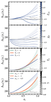 |
Fig. 6. Virial overdensity for phenomenological models. |
6.3. Case with wΛ≠−1
When we modify the nature of dark energy itself by assuming a kind of non-standard EoS, we need to tweak previously introduced expressions. As noted in Wang & Steinhardt (1998), for quintessence cosmology, the virial theorem has an additional term:
The potential energy contribution for DE is given by 〈UΛ〉=−4/5πGρΛMR2. For the wΛCDM model, dark energy does not cluster, and thus Birkhoff's theorem remains valid. Hence, the radius evolution is governed by
This is very similar to the Eq. (98), derived for phenomenological modified gravity. We assume that wΛ≠−1, with a constant EoS parameter. The corresponding dark energy density is  . This can be inferred from the usual conservation equation in the absence of interactions between sectors. Since dark energy contributes to spherical collapse only on the background level, its terms in Eq. (108) are absorbed into the Hubble parameter using the second Friedmann equation.
We derive Δvir using the expression for radius from Eq. (108) and the same initial conditions that were assumed in the phenomenological scenario. The radius is substituted into the virial theorem based on Eqs. (100) and (101). The results are then plotted in Figure 7.
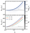 |
Fig. 7. Virial overdensity for the theories of modified gravitation with the screening field present, namely, nDGP and k-mouflage. |
6.4. Case with the present screening field
In order to preserve the cosmological principle, for both nDGP and k-mouflage cosmologies an additional scalar field must be introduced. Due to the coupling between the scalar field with gravity, some additional terms will arise in the radius evolution equation. As shown in Schmidt et al. (2010), we get
Interestingly, the virial condition itself remains unchanged. For screened gravity, kinetic energy is the same as in phenomenological models (see Eq. (100)). On the contrary, the potential energy is modified
The virial radius is then defined using the approach laid out in Section 6.2. Minimal halo mass is expressed by Eq. (106), under the change of variables μ→Geff(R/R★)/GN. This result is valid for nDGP. However, since the notion of screening for k-mouflage differs from nDGP (see Eq. (62)), we have to make an appropriate change for k-mouflage, as discussed in Brax & Valageas (2014a). We note that for k-mouflage, at scales ctk/a≫1, screening can be neglected. For small enough redshift, these scales correspond to ∼Mpc, at which galaxy clusters reside. For example, a Coma cluster with radius R∼20 Mpc (upper limit from Chernin et al. 2013) lies within the range of unscreened gravity. Thus, ignoring the effects of screening, we can introduce the equation for radius evolution within k-mouflage theory as follows (Brax & Valageas 2014a):
Here,  is a non-linear quantity, constructed from its background and perturbed components. The background contribution is calculated from Eq. (31) and the perturbed contribution arises due to δφ. We can then derive a Bardeen potential using the modified Poisson equation (Brax & Valageas 2014a):
From BBN constraints, we obtain A≃1 and ℬ≃β (Brax & Valageas 2014a). It is important to note that Eq. (112) is valid only for the case when δnl≲200. This is suitable for computing virial quantities. However, it will fail at smaller scales, such as those corresponding to the Milky Way core or the Solar System, where GR should be restored via the screening mechanism absent from the aforementioned equation. Therefore, we set the non-linear density threshold at the time of spherical collapse to δnl = 200, which has been shown to be an effective choice for the derivation of the halo mass function (for instance, see Brax et al. (2015)). Using the prescription outlined in Brax & Valageas (2014a), we rearrange Eq. (111), and define a new variable,  . An obvious initial condition for the radius is to take
  . This variable is related to the non-linear density contrast via δnl+1=y(t)−3. This expression for non-linear density contrast was then substituted into the Eq. (111) to get the following differential equation:
In Brax et al. (2015), it was demonstrated that the k-mouflage gravitational potential differs from ΛCDM by a factor of μ(a) = 1+ϵ1(a). Since there is no explicit radius dependence in μ for k-mouflage, the computation of kinetic and potential energies is very similar to the phenomenological gravity discussed earlier.
We plot the numerical solutions for both nDGP and k-mouflage for Δvir in Figure (7). Interestingly, similar to the phenomenological case, for screened theories, Δvir(ac)→18π2 as ac→0. This is not a trivial result, as screened theories modify not only the effective dark energy but also add some additional matter terms to the respective Lagrangians that can decay at a different rate compared to the dark energy component, hence possess a non-zero mass fraction at a higher redshift. The consequence of this is that in some cases deviations from ΛCDM can be observed at very high redshifts.
With the help of the virial radius, we then obtained the virial temperature using Eq. (95). This allowed us to place a lower bound on halo mass, at which the gas within the halo can cool efficiently. Mmin is then substituted into Eq. (91) to derive the hydrogen ionisation fractions. Theoretical predictions for QHII(z) and τreion(z) are subsequently compared to the observational data in the next section.
7. Discussion and concluding remarks
Most of the constraints and best-fit parameters for SMF, SMD, SFRD, and UVLF, EoR have already been thoroughly discussed in Appendix A. We show the compilation of all of those results for screened theories of modified gravity in Figure 8. We note that in some cases, a second solution was found (i.e. the solution is degenerate). This has been indicated in Figure 8 using circle and square markers. Upper limits are indicated where appropriate. Such a degeneracy appears to be due to the fact that the variation of β can increase the abundance of galaxies and K0 can decrease it. Thus, it is possible to find several similar solutions for different choices of a pair {β,K0}. The fact that we only found two degenerate solutions at most is because we have considered a coarse grid for β; hence, there will be more degenerate solutions for a grid of higher resolution.
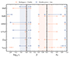 |
Fig. 8. Compilation of the best-fit parameters determined by the visual inspection of various observables for nDGP (first column) and k-mouflage (second and third columns). Arrows signify an upper limit for a parameter, while shaded areas represent the parameter space preferred by the vast majority of observational datasets. |
In Figure 8, we can see that the choice of rc∼103.9 Mpc can provide the best fitting predictions for a wide range of observables and both stellar mass to halo relations. A similar situation may be observed in the case of k-mouflage, where β∼0.1, K0≳0.9 is highly preferred for the double power-law SMHR and β∼0.3, K0≲0.3 for Rodriguez-Puebla. Figure 8 does not illustrate the results for the phenomenological theories, specifically for wγCDM, due the incomplete set of constraints, but it is worth mentioning that this model prefers wΛ≲−1 (i.e. phantom or ΛCDM cosmology) instead of quintessence when using both SMF and SFRD. For other phenomenological theories, we have not found a substantial preference for a single parameter choice. We conclude that phenomenological theories cannot be stringently constrained with the help of quantities considered in the current work, mainly because phenomenological theories provide only a very slight deviation from the ΛCDM on the background level. It may be interesting to couple star formation probes with the constraints from CMB and BAO, observe if the situation is any different. The only quantity that suggests the need for a substantial deviation from ΛCDM is the stellar mass density. It is interesting to note that the double power-law best-fit values are noticeably closer to the ΛCDM than Rodriguez-Puebla. This is an important result because it highlights the sensitivity of the adopted star formation history model as a test for new physics.
Another important result from the calculations described in this work is that whilst all other models fail, the k-mouflage theory with the double-power law SMHR can satisfy both reionisation and high-redshift SMD constraints imposed by the JWST up to M★∼1011 M⊙. We note that the warm dark matter prescription of Gong et al. (2023) also achieves this. The reason that both phenomenological and nDGP theories fail (in this context) is that changes in QHII(z) within those theories are too small to provide good fits to the observational data. Even if it was possible to satisfy reionisation constraints in the nDGP case, Figure A.8 shows that the observed SMD can only be reproduced for rc≲102.5 Mpc, which is way outside the observational bound, making this choice nonviable.
The theories we have considered are only able to satisfactorily fit the observational SMF and UVLF if the UVLF to stellar mass relation has additional scatter over and above that depicted in Equation 88. As previously discussed, this is most probably due to the fact that the SMHRs considered in this work have been calibrated on different datasets. This problem has been addressed in a more recent work Behroozi et al. (2019), where the authors combine SFR, UVLF, and SMF measurements to deduce the SMHR. Figure 8 shows several discrepancies between the model parameter estimates obtained using the Rodriguez-Puebla and double-power law SMHR, for example, the Planck2018 τreion parameter measurement. In that example, the discrepancy is a consequence of the Rodriguez-Puebla SMHR being calibrated using SFR/SMD data, whilst the double-power law was calibrated using UVLF data. The estimated τreion parameter will depend on both the additional scatter between the UVLF and the SMF and the form used for  . As noted by Finkelstein et al. (2019), the rate of production of Ly-C photons can also be defined in terms of the ultraviolet luminosity density. Compared to ΛCDM, the nDGP and k-mouflage theories always lead to an overabundance of UV sources and stellar mass overestimates. However, JWST data suggests that regardless of whether we use Rodriguez-Puebla or the double power-law, we need fewer sources than predicted by ΛCDM at high redshifts (e.g., see Figure A.5). In general, both phenomenological, screened, and ΛCDM cosmologies are ruled out by the newest JWST data if one will try to satisfy both SMD and SMF (or analogously, SMD and UVLF). This is a serious issue that can probably be addressed by changing the star formation prescription to something more sophisticated.
Even though we have taken into account several sources of scatter, it is possible that additional uncertainties are present that contribute to the scatter seen in the results presented in Figure 8. One example of a potential additional error source is the escape fraction of photons, namely, fesc. Throughout the literature, various values for fesc have been assumed, and there is no verdict on which assumption is the most correct, as it is not something that can be directly observed. Hence, the variation of fesc will lead to the variation of reionisation quantities, which in turn will change the constrained parameter space.
Other parameters, such as ϵ★,0, are not bounded at all. We had to assume the ΛCDM value in these cases. This is motivated by the fact that ΛCDM prediction of the SMF ‘should’ be close to the observational data, which has been confirmed by the cosmological observations, but one can still keep it as a free parameter for the sake of generality.
Another possible issue is that we have assumed a Planck2018 cosmology that was established with ΛCDM as a background. In a perfect scenario, one will include cosmological parameters such as H0 or Ωm0 into the analysis as free variables. However, doing so is impractical in terms of the computing time required.
Currently, there are several constraints imposed on the nDGP gravity in the literature. For example, correlation function monopole and quadrupole, obtained from the SDSS DR7 sample, suggest that rc>102.53 Mpc at a 2σ confidence (Raccanelli et al. 2013). However, analysis of the DR11 sample has a stricter constraint of rc>103.65 Mpc (Barreira et al. 2016), which is very close to what we derive. We are not aware of constraints for the pair {β,K0} within the k-mouflage theory using the parameterisation that we have assumed. However, a recent study using mock observations of Stage IV cosmic shear surveys Frusciante et al. (2024) may lead to interesting constraints on nDGP and k-mouflage theories.
The main purpose of the work described in this paper is to put forward new ideas as to how one might use new astronomical observations to constrain interesting theories of gravity beyond GR. Clearly, a great deal of further work is required to identify the most effective ways one may realise this task. For example, after further optimisation of our code, one could run more detailed Markov chain Monte Carlo calculations using thousands of steps in parameter space. This would then enable the redshift evolution of the preferred value of σUV (and its uncertainty) to be determined as a function of the relevant modified gravity free parameter. It may even be possible to make parameters such as the photon escape fraction fesc or the double power-law SMHR slopes γlo, γhi free variables and derive the constraints for them. Whilst this exact approach has been used within the framework of ΛCDM (Ren et al. 2019), the redshift evolution of those parameters will change significantly with the introduction of screened gravity due to the differences in the structure formation prescriptions. Hence, the evolution of SMHR slopes with the redshift may serve as another indicator of the viability of a particular theory of gravity.
Data availability
We have made the codes available via the link GITHUB. We note that the code was made for internal use and therefore is poorly commented. For any questions, contact to the corresponding author. All ΛCDM results produced by the code have been carefully checked for consistency with the data available in the literature to make sure that the code is working properly. For SMF/SMD comparison, we have used the data from Dayal & Giri (2023), Gong et al. (2023), for UVLF we have used Shen et al. (2023) and for spherical collapse, Pace et al. (2010). Only small deviations have been observed for some quantities, and we believe that they arise due to the numerical precision limitations (for example, the size of the interpolation grid for the scale factor used to find spherical collapse initial conditions) and different cosmology assumed (for example, WMAP9 instead of Planck2018).
Acknowledgments
I am grateful to Prof. John Webb for a fruitful discussion and insightful comments on this work. Sokoliuk O. performed the work in frame of the “Mathematical modeling in interdisciplinary research of processes and systems based on intelligent supercomputer, grid and cloud technologies” program of the NAS of Ukraine. This article/publication is based upon work from COST Action CA21136 “Addressing observational tensions in cosmology with systematics and fundamental physics (CosmoVerse)” supported by COST (European Cooperation in Science and Technology). In addition, this work has also benefited from the use of open-source Python packages: SciPy (Virtanen et al. 2020), Matplotlib (Hunter 2007), NumPy (Harris et al. 2020) and emcee (Foreman-Mackey et al. 2013). Parts of the Pylians3 code (Villaescusa-Navarro 2018) were used to implement HMF derivation.
References
- Abdalla, E., Abellán, G. F., Aboubrahim, A., et al. 2022, J. High Energy Astrophys., 34, 49 [NASA ADS] [CrossRef] [Google Scholar]
- Abramo, L. R., Batista, R. C., Liberato, L., & Rosenfeld, R. 2007, JCAP, 2007, 012 [Google Scholar]
- Ade, P. A. R., Aghanim, N., Arnaud, M., et al. 2016, A&A, 594, A14 [NASA ADS] [CrossRef] [EDP Sciences] [Google Scholar]
- Adil, S. A., Mukhopadhyay, U., Sen, A. A., & Vagnozzi, S. 2023, JCAP, 2023, 072 [Google Scholar]
- Albuquerque, I. S., Frusciante, N., Pace, F., & Schimd, C. 2024, Phys. Rev. D, 109, 023535 [Google Scholar]
- Amendola, L., Kunz, M., & Sapone, D. 2008, JCAP, 2008, 013 [Google Scholar]
- Amendola, L., Kunz, M., Motta, M., Saltas, I. D., & Sawicki, I. 2013, Phys. Rev. D, 87, 023501 [Google Scholar]
- Anchordoqui, L. A., Di Valentino, E., Pan, S., & Yang, W. 2021, J. High Energy Astrophys., 32, 28 [NASA ADS] [CrossRef] [Google Scholar]
- Arjona, R., Cardona, W., & Nesseris, S. 2019, Phys. Rev. D, 99, 043516 [NASA ADS] [CrossRef] [Google Scholar]
- Asencio, E., Banik, I., & Kroupa, P. 2021, MNRAS, 500, 5249 [Google Scholar]
- Avilez, A., & Skordis, C. 2014, Phys. Rev. Lett., 113, 011101 [CrossRef] [Google Scholar]
- Babichev, E., Deffayet, C., & Ziour, R. 2009, Int. J. Mod. Phys. D, 18, 2147 [NASA ADS] [CrossRef] [Google Scholar]
- Baker, T., Barreira, A., Desmond, H., et al. 2019, ArXiv e-prints [arXiv:1908.03430] [Google Scholar]
- Baldry, I. K., Driver, S. P., Loveday, J., et al. 2012, MNRAS, 421, 621 [NASA ADS] [Google Scholar]
- Barkana, R., & Loeb, A. 2001, Phys. Rep., 349, 125 [NASA ADS] [CrossRef] [Google Scholar]
- Barreira, A., Sánchez, A. G., & Schmidt, F. 2016, Phys. Rev. D, 94, 084022 [NASA ADS] [CrossRef] [Google Scholar]
- Barrow, J. D., & Magueijo, J. 1999, CQG, 16, 1435 [Google Scholar]
- Behroozi, P. S., Conroy, C., & Wechsler, R. H. 2010, ApJ, 717, 379 [Google Scholar]
- Behroozi, P. S., Wechsler, R. H., & Conroy, C. 2013, ApJ, 770, 57 [NASA ADS] [CrossRef] [Google Scholar]
- Behroozi, P., Wechsler, R. H., Hearin, A. P., & Conroy, C. 2019, MNRAS, 488, 3143 [NASA ADS] [CrossRef] [Google Scholar]
- Bell, E. F., McIntosh, D. H., Katz, N., & Weinberg, M. D. 2003, ApJS, 149, 289 [Google Scholar]
- Bellini, E., Bartolo, N., & Matarrese, S. 2012, JCAP, 2012, 019 [CrossRef] [Google Scholar]
- Benevento, G., Raveri, M., Lazanu, A., et al. 2019, JCAP, 2019, 027 [CrossRef] [Google Scholar]
- Bengochea, G. R., & Ferraro, R. 2009, Phys. Rev. D, 79, 124019 [Google Scholar]
- Bertschinger, E. 2006, ApJ, 648, 797 [Google Scholar]
- Bhatawdekar, R., Conselice, C. J., Margalef-Bentabol, B., & Duncan, K. 2019, MNRAS, 486, 3805 [NASA ADS] [CrossRef] [Google Scholar]
- Boettner, C., Trebitsch, M., & Dayal, P. 2025, A&A, 693, A295 [NASA ADS] [CrossRef] [EDP Sciences] [Google Scholar]
- Boissier, S. 2013, in Planets, Stars and Stellar Systems. Volume 6: Extragalactic Astronomy and Cosmology, eds. T. D. Oswalt, & W. C. Keel, 6, 141 [NASA ADS] [CrossRef] [Google Scholar]
- Bolan, P., Lemaux, B. C., Mason, C., et al. 2022, MNRAS, 517, 3263 [Google Scholar]
- Borde, A., Guth, A. H., & Vilenkin, A. 2003, Phys. Rev. Lett., 90, 151301 [Google Scholar]
- Bouwens, R., Illingworth, G., Oesch, P., et al. 2023a, MNRAS, 523, 1009 [NASA ADS] [CrossRef] [Google Scholar]
- Bouwens, R. J., Stefanon, M., Brammer, G., et al. 2023b, MNRAS, 523, 1036 [NASA ADS] [CrossRef] [Google Scholar]
- Boylan-Kolchin, M. 2023, Nat. Astron., 7, 731 [NASA ADS] [CrossRef] [Google Scholar]
- Brammer, G. B., Whitaker, K. E., van Dokkum, P. G., et al. 2011, ApJ, 739, 24 [NASA ADS] [CrossRef] [Google Scholar]
- Brax, P., & Valageas, P. 2014a, Phys. Rev. D, 90, 023508 [NASA ADS] [CrossRef] [Google Scholar]
- Brax, P., & Valageas, P. 2014b, Phys. Rev. D, 90, 023507 [Google Scholar]
- Brax, P., & Valageas, P. 2014c, Phys. Rev. D, 90, 123521 [Google Scholar]
- Brax, P., & Valageas, P. 2016, JCAP, 01, 020 [CrossRef] [Google Scholar]
- Brax, P., Rizzo, L. A., & Valageas, P. 2015, Phys. Rev. D, 92, 043519 [NASA ADS] [CrossRef] [Google Scholar]
- Buchert, T., Coley, A. A., Kleinert, H., Roukema, B. F., & Wiltshire, D. L. 2016, Int. J. Mod. Phys. D, 25, 1630007 [Google Scholar]
- Carucci, I. P., & Corasaniti, P. -S. 2019, Phys. Rev. D, 99, 023518 [NASA ADS] [CrossRef] [Google Scholar]
- Chernin, A. D., Bisnovatyi-Kogan, G. S., Teerikorpi, P., et al. 2013, A&A, 553, A101 [NASA ADS] [CrossRef] [EDP Sciences] [Google Scholar]
- Choudhury, T. R. 2022, General Relativ. Gravitation, 54, 102 [Google Scholar]
- Chworowsky, K., Finkelstein, S. L., Boylan-Kolchin, M., et al. 2023, ArXiv e-prints [arXiv:2311.14804] [Google Scholar]
- Cognola, G., Elizalde, E., Nojiri, S., Odintsov, S. D., & Zerbini, S. 2006, Phys. Rev. D, 73, 084007 [Google Scholar]
- Cole, S., Norberg, P., Baugh, C. M., et al. 2001, MNRAS, 326, 255 [NASA ADS] [CrossRef] [Google Scholar]
- Conroy, C., & Wechsler, R. H. 2009, ApJ, 696, 620 [NASA ADS] [CrossRef] [Google Scholar]
- Correa, C. A., Wyithe, J. S. B., Schaye, J., & Duffy, A. R. 2015a, MNRAS, 450, 1514 [NASA ADS] [CrossRef] [Google Scholar]
- Correa, C. A., Wyithe, J. S. B., Schaye, J., & Duffy, A. R. 2015b, MNRAS, 450, 1521 [NASA ADS] [CrossRef] [Google Scholar]
- Croft, R. A. C., Weinberg, D. H., Bolte, M., et al. 2002, ApJ, 581, 20 [NASA ADS] [CrossRef] [Google Scholar]
- Cullen, F., McLure, R. J., McLeod, D. J., et al. 2023, MNRAS, 520, 14 [NASA ADS] [CrossRef] [Google Scholar]
- Davies, F. B., Hennawi, J. F., Bañados, E., et al. 2018, ApJ, 864, 142 [NASA ADS] [CrossRef] [Google Scholar]
- Dayal, P., & Giri, S. K. 2023, ArXiv e-prints [arXiv:2303.14239] [Google Scholar]
- Del Popolo, A., Gambera, M., & Antonuccio-Delogu, V. 1998, AAT, 16, 127 [Google Scholar]
- Dhoke, P., & Paranjape, A. 2021, MNRAS, 508, 852 [Google Scholar]
- Di Valentino, E. 2021, MNRAS, 502, 2065 [CrossRef] [Google Scholar]
- Di Valentino, E., Mena, O., Pan, S., et al. 2021, CQG, 38, 153001 [NASA ADS] [CrossRef] [Google Scholar]
- Dijkstra, M., Lidz, A., & Wyithe, J. S. B. 2007, MNRAS, 377, 1175 [NASA ADS] [CrossRef] [Google Scholar]
- Donnan, C. T., McLeod, D. J., Dunlop, J. S., et al. 2023, MNRAS, 518, 6011 [Google Scholar]
- Drory, N., Bundy, K., Leauthaud, A., et al. 2009, ApJ, 707, 1595 [NASA ADS] [CrossRef] [Google Scholar]
- Duncan, K., Conselice, C. J., Mortlock, A., et al. 2014, MNRAS, 444, 2960 [Google Scholar]
- Dvali, G., Gabadadze, G., & Porrati, M. 2000, Phys. Lett. B, 485, 208 [Google Scholar]
- Eldridge, J. J., Stanway, E. R., Xiao, L., et al. 2017, PASA, 34, e058 [Google Scholar]
- Engineer, S., Kanekar, N., & Padmanabhan, T. 2000, MNRAS, 314, 279 [Google Scholar]
- Esposito-Farèse, G., & Polarski, D. 2001, Phys. Rev. D, 63, 063504 [CrossRef] [Google Scholar]
- Fernandez, R., Bryan, G. L., Haiman, Z., & Li, M. 2014, MNRAS, 439, 3798 [CrossRef] [Google Scholar]
- Fields, B. D. 2011, Ann. Rev. Nucl. Part. Sci., 61, 47 [Google Scholar]
- Finkelstein, S. L., D’Aloisio, A., Paardekooper, J. -P., et al. 2019, ApJ, 879, 36 [NASA ADS] [CrossRef] [Google Scholar]
- Finkelstein, S. L., Bagley, M. B., Ferguson, H. C., et al. 2023, ApJ, 946, L13 [NASA ADS] [CrossRef] [Google Scholar]
- Foreman-Mackey, D., Hogg, D. W., Lang, D., & Goodman, J. 2013, PASP, 125, 306 [Google Scholar]
- Frusciante, N., Pace, F., Cardone, V. F., et al. 2024, A&A, 690, A133 [NASA ADS] [CrossRef] [EDP Sciences] [Google Scholar]
- Fudamoto, Y., Oesch, P. A., Schouws, S., et al. 2021, Nature, 597, 489 [CrossRef] [Google Scholar]
- Furlong, M., Bower, R. G., Theuns, T., et al. 2015, MNRAS, 450, 4486 [Google Scholar]
- Gaikwad, P., Haehnelt, M. G., Davies, F. B., et al. 2023, MNRAS, 525, 4093 [NASA ADS] [CrossRef] [Google Scholar]
- Gelli, V., Mason, C., & Hayward, C. C. 2024, ArXiv e-prints [arXiv:2405.13108] [Google Scholar]
- Gen, U., Ishibashi, A., & Tanaka, T. 2002, Phys. Rev. D, 66, 023519 [Google Scholar]
- Glazebrook, K., Nanayakkara, T., Schreiber, C., et al. 2023, ArXiv e-prints [arXiv:2308.05606] [Google Scholar]
- Gnedin, N. Y., & Hamilton, A. J. S. 2002, MNRAS, 334, 107 [Google Scholar]
- Gnedin, N. Y., & Madau, P. 2022, Liv. Rev. Comput. Astrophys., 8, 3 [CrossRef] [Google Scholar]
- Gong, Y., Yue, B., Cao, Y., & Chen, X. 2023, ApJ, 947, 28 [NASA ADS] [CrossRef] [Google Scholar]
- Greig, B., Mesinger, A., Davies, F. B., et al. 2022, MNRAS, 512, 5390 [NASA ADS] [CrossRef] [Google Scholar]
- Guszejnov, D., Grudić, M. Y., Offner, S. S. R., et al. 2022, MNRAS, 515, 4929 [Google Scholar]
- Harikane, Y., Ouchi, M., Oguri, M., et al. 2023, ApJS, 265, 5 [NASA ADS] [CrossRef] [Google Scholar]
- Harris, C. R., Millman, K. J., van der Walt, S. J., et al. 2020, Nature, 585, 357 [NASA ADS] [CrossRef] [Google Scholar]
- Hassan, S., Davé, R., McQuinn, M., et al. 2022, ApJ, 931, 62 [NASA ADS] [CrossRef] [Google Scholar]
- Hernández-Aguayo, C., Arnold, C., Li, B., & Baugh, C. M. 2021, MNRAS, 503, 3867 [Google Scholar]
- Hirano, S., & Yoshida, N. 2023, ArXiv e-prints [arXiv:2306.11993] [Google Scholar]
- Hoag, A., Bradač, M., Huang, K., et al. 2019, ApJ, 878, 12 [NASA ADS] [CrossRef] [Google Scholar]
- Hu, Y., Turner, M. S., & Weinberg, E. J. 1994, Phys. Rev. D, 49, 3830 [Google Scholar]
- Hunter, J. D. 2007, Comput. Sci. Eng., 9, 90 [NASA ADS] [CrossRef] [Google Scholar]
- Inayoshi, K., Harikane, Y., Inoue, A. K., Li, W., & Ho, L. C. 2022, ApJ, 938, L10 [NASA ADS] [CrossRef] [Google Scholar]
- Kaluza, T. 1921, Sitzungsberichte der Königlich Preussischen Akademie der Wissenschaften, 966 [Google Scholar]
- Kaurov, A. A., & Gnedin, N. Y. 2015, ApJ, 810, 154 [Google Scholar]
- Khaire, V., Srianand, R., Choudhury, T. R., & Gaikwad, P. 2016, MNRAS, 457, 4051 [CrossRef] [Google Scholar]
- Kikuchihara, S., Ouchi, M., Ono, Y., et al. 2020, ApJ, 893, 60 [NASA ADS] [CrossRef] [Google Scholar]
- Kim, J. -G., Ostriker, E. C., & Filippova, N. 2021, ApJ, 911, 128 [NASA ADS] [CrossRef] [Google Scholar]
- Kimura, R., & Yamamoto, K. 2011, JCAP, 2011, 025 [CrossRef] [Google Scholar]
- Klein, O. 1926, Z. Phys., 37, 895 [Google Scholar]
- Konno, A., Ouchi, M., Ono, Y., et al. 2014, ApJ, 797, 16 [Google Scholar]
- Konno, A., Ouchi, M., Shibuya, T., et al. 2018, PASJ, 70, S16 [Google Scholar]
- Koyama, K. 2016, Rep. Prog. Phys., 79, 046902 [NASA ADS] [CrossRef] [Google Scholar]
- Koyama, K., & Maartens, R. 2006, JCAP, 2006, 016 [NASA ADS] [CrossRef] [Google Scholar]
- Koyama, K., & Silva, F. P. 2007, Phys. Rev. D, 75, 084040 [NASA ADS] [CrossRef] [Google Scholar]
- Kuhlen, M., & Faucher-Giguère, C. -A. 2012, MNRAS, 423, 862 [NASA ADS] [CrossRef] [Google Scholar]
- Labbé, I., van Dokkum, P., Nelson, E., et al. 2023, Nature, 616, 266 [CrossRef] [Google Scholar]
- Lahav, O., Lilje, P. B., Primack, J. R., & Rees, M. J. 1991, MNRAS, 251, 128 [Google Scholar]
- Leauthaud, A., Bundy, K., Saito, S., et al. 2016, MNRAS, 457, 4021 [Google Scholar]
- Lee, J., Shin, J., Snaith, O. N., et al. 2021, ApJ, 908, 11 [CrossRef] [Google Scholar]
- Leitherer, C., Schaerer, D., Goldader, J. D., et al. 1999, ApJS, 123, 3 [Google Scholar]
- Leo, M., Baugh, C. M., Li, B., & Pascoli, S. 2018, JCAP, 04, 010 [Google Scholar]
- Lesgourgues, J. 2011, ArXiv e-prints [arXiv:1104.2932] [Google Scholar]
- Leung, G. C. K., Bagley, M. B., Finkelstein, S. L., et al. 2023, ApJ, 954, L46 [NASA ADS] [CrossRef] [Google Scholar]
- Lewis, A., Challinor, A., & Lasenby, A. 2000, ApJ, 538, 473 [Google Scholar]
- L’Huillier, B., Shafieloo, A., & Kim, H. 2018, MNRAS, 476, 3263 [Google Scholar]
- Lightman, A. P., & Schechter, P. L. 1990, ApJS, 74, 831 [NASA ADS] [CrossRef] [Google Scholar]
- Lombriser, L., Hu, W., Fang, W., & Seljak, U. 2009, Phys. Rev. D, 80, 063536 [CrossRef] [Google Scholar]
- Lombriser, L., Li, B., Koyama, K., & Zhao, G. -B. 2013, Phys. Rev. D, 87, 123511 [NASA ADS] [CrossRef] [Google Scholar]
- Maartens, R., & Koyama, K. 2010, Liv. Rev. Relativity, 13, 5 [Google Scholar]
- Madau, P., & Dickinson, M. 2014, ARA&A, 52, 415 [Google Scholar]
- Madau, P., Haardt, F., & Rees, M. J. 1999, ApJ, 514, 648 [CrossRef] [Google Scholar]
- Malekjani, M., Naderi, T., & Pace, F. 2015, MNRAS, 453, 4148 [Google Scholar]
- Malekjani, M., Haidari, N., & Basilakos, S. 2017, MNRAS, 466, 3488 [Google Scholar]
- Marchesini, D., van Dokkum, P. G., Förster Schreiber, N. M., et al. 2009, ApJ, 701, 1765 [NASA ADS] [CrossRef] [Google Scholar]
- Marsh, M. C. D., McAllister, L., Pajer, E., & Wrase, T. 2013, JCAP, 2013, 040 [Google Scholar]
- Martin, J. 2012, Comptes Rendus Phys., 13, 566 [Google Scholar]
- McBride, J., Fakhouri, O., & Ma, C. -P. 2009, MNRAS, 398, 1858 [NASA ADS] [CrossRef] [Google Scholar]
- McGreer, I. D., Mesinger, A., & D’Odorico, V. 2015, MNRAS, 447, 499 [NASA ADS] [CrossRef] [Google Scholar]
- Mendel, J. T., Simard, L., Palmer, M., Ellison, S. L., & Patton, D. R. 2014, ApJS, 210, 3 [Google Scholar]
- Meurer, G. R., Heckman, T. M., & Calzetti, D. 1999, ApJ, 521, 64 [Google Scholar]
- Mirocha, J., Furlanetto, S. R., & Sun, G. 2017, MNRAS, 464, 1365 [NASA ADS] [CrossRef] [Google Scholar]
- Mirocha, J., Lamarre, H., & Liu, A. 2021, MNRAS, 504, 1555 [Google Scholar]
- Moffat, J. W., & Toth, V. T. 2009, MNRAS, 395, L25 [Google Scholar]
- Mortlock, A., Conselice, C. J., Bluck, A. F. L., et al. 2011, MNRAS, 413, 2845 [Google Scholar]
- Moster, B. P., Somerville, R. S., Maulbetsch, C., et al. 2010, ApJ, 710, 903 [Google Scholar]
- Muñoz, J. B., Mirocha, J., Chisholm, J., Furlanetto, S. R., & Mason, C. 2024, MNRAS, submitted [arXiv:2404.07250] [Google Scholar]
- Naidu, R. P., Oesch, P. A., van Dokkum, P., et al. 2022, ApJ, 940, L14 [NASA ADS] [CrossRef] [Google Scholar]
- Navarro-Carrera, R., Rinaldi, P., Caputi, K. I., et al. 2024, ApJ, 961, 207 [CrossRef] [Google Scholar]
- Nebrin, O. 2023, Res. Notes Am. Astron. Soc., 7, 90 [Google Scholar]
- Neistein, E., van den Bosch, F. C., & Dekel, A. 2006, MNRAS, 372, 933 [NASA ADS] [CrossRef] [Google Scholar]
- Nesseris, S., & Sapone, D. 2015, Phys. Rev. D, 92, 023013 [Google Scholar]
- Nesseris, S., Pantazis, G., & Perivolaropoulos, L. 2017, Phys. Rev. D, 96, 023542 [Google Scholar]
- Nojiri, S., & Odintsov, S. D. 2003, Phys. Rev. D, 68, 123512 [Google Scholar]
- Nojiri, S., & Odintsov, S. D. 2011, Phys. Rep., 505, 59 [CrossRef] [Google Scholar]
- Nojiri, S., Odintsov, S. D., & Oikonomou, V. K. 2017, Phys. Rep., 692, 1 [NASA ADS] [CrossRef] [Google Scholar]
- Pace, F., Waizmann, J. C., & Bartelmann, M. 2010, MNRAS, 406, 1865 [Google Scholar]
- Pace, F., Meyer, S., & Bartelmann, M. 2017, JCAP, 2017, 040 [CrossRef] [Google Scholar]
- Pakmor, R., Springel, V., Coles, J. P., et al. 2023, MNRAS, 524, 2539 [NASA ADS] [CrossRef] [Google Scholar]
- Parimbelli, G., Scelfo, G., Giri, S. K., et al. 2021, JCAP, 2021, 044 [CrossRef] [Google Scholar]
- Pérez-González, P. G., Rieke, G. H., Villar, V., et al. 2008, ApJ, 675, 234 [Google Scholar]
- Pérez-González, P. G., Costantin, L., Langeroodi, D., et al. 2023, ApJ, 951, L1 [CrossRef] [Google Scholar]
- Perivolaropoulos, L., & Skara, F. 2022, New Astron. Rev., 95, 101659 [CrossRef] [Google Scholar]
- Planck Collaboration VI. 2020, A&A, 641, A6 [NASA ADS] [CrossRef] [EDP Sciences] [Google Scholar]
- Pogosian, L., Silvestri, A., Koyama, K., & Zhao, G. -B. 2010, Phys. Rev. D, 81, 104023 [NASA ADS] [CrossRef] [Google Scholar]
- Posti, L., Fraternali, F., & Marasco, A. 2019, A&A, 626, A56 [NASA ADS] [CrossRef] [EDP Sciences] [Google Scholar]
- Pozzetti, L., Bolzonella, M., Zucca, E., et al. 2010, A&A, 523, A13 [NASA ADS] [CrossRef] [EDP Sciences] [Google Scholar]
- Press, W. H., & Schechter, P. 1974, ApJ, 187, 425 [Google Scholar]
- Price, L. C., Trac, H., & Cen, R. 2016, ArXiv e-prints [arXiv:1605.03970] [Google Scholar]
- Raccanelli, A., Bertacca, D., Pietrobon, D., et al. 2013, MNRAS, 436, 89 [NASA ADS] [CrossRef] [Google Scholar]
- Randall, L., & Sundrum, R. 1999, Phys. Rev. Lett., 83, 4690 [Google Scholar]
- Ren, K., Trenti, M., & Mason, C. A. 2019, ApJ, 878, 114 [Google Scholar]
- Riess, A. G., Filippenko, A. V., Challis, P., et al. 1998, AJ, 116, 1009 [Google Scholar]
- Robertson, B. E., Furlanetto, S. R., Schneider, E., et al. 2013, ApJ, 768, 71 [Google Scholar]
- Robertson, B. E., Ellis, R. S., Furlanetto, S. R., & Dunlop, J. S. 2015, ApJ, 802, L19 [Google Scholar]
- Rodríguez-Puebla, A., Primack, J. R., Avila-Reese, V., & Faber, S. M. 2017, MNRAS, 470, 651 [Google Scholar]
- Ruiz-Zapatero, J., García-García, C., Alonso, D., Ferreira, P. G., & Grumitt, R. D. P. 2022, MNRAS, 512, 1967 [Google Scholar]
- Sakr, Z., & Martinelli, M. 2022, JCAP, 2022, 030 [Google Scholar]
- Salcido, J., Bower, R. G., & Theuns, T. 2020, MNRAS, 491, 5083 [NASA ADS] [CrossRef] [Google Scholar]
- Santini, P., Fontana, A., Castellano, M., et al. 2023, ApJ, 942, L27 [NASA ADS] [CrossRef] [Google Scholar]
- Saridakis, E. N., Lazkoz, R., Salzano, V., et al. 2021, ArXiv e-prints [arXiv: arXiv:2105.12582] [Google Scholar]
- Schive, H. -Y., Chiueh, T., Broadhurst, T., & Huang, K. -W. 2016, ApJ, 818, 89 [NASA ADS] [CrossRef] [Google Scholar]
- Schmidt, F. 2009, Phys. Rev. D, 80, 123003 [NASA ADS] [CrossRef] [Google Scholar]
- Schmidt, F., Lima, M., Oyaizu, H., & Hu, W. 2009, Phys. Rev. D, 79, 083518 [NASA ADS] [CrossRef] [Google Scholar]
- Schmidt, F., Hu, W., & Lima, M. 2010, Phys. Rev. D, 81, 063005 [Google Scholar]
- Shen, X., Vogelsberger, M., Boylan-Kolchin, M., Tacchella, S., & Kannan, R. 2023, MNRAS, 525, 3254 [NASA ADS] [CrossRef] [Google Scholar]
- Shen, X., Vogelsberger, M., Boylan-Kolchin, M., Tacchella, S., & Naidu, R. P. 2024, ArXiv e-prints [arXiv:2406.15548] [Google Scholar]
- Shen, X., Borrow, J., Vogelsberger, M., et al. 2024b, MNRAS, 527, 2835 [Google Scholar]
- Sheth, R. K., & Tormen, G. 1999, MNRAS, 308, 119 [Google Scholar]
- Silk, J., & Mamon, G. A. 2012, Res. Astron. Astrophys., 12, 917 [Google Scholar]
- Song, M., Finkelstein, S. L., Ashby, M. L. N., et al. 2016, ApJ, 825, 5 [NASA ADS] [CrossRef] [Google Scholar]
- Specogna, E., Di Valentino, E., Said, J. L., & Nguyen, N. -M. 2024, Phys. Rev. D, 109, 043528 [Google Scholar]
- Starobinsky, A. A. 1980, Phys. Lett. B, 91, 99 [Google Scholar]
- Stefanon, M., Bouwens, R. J., Labbé, I., et al. 2021, ApJ, 922, 29 [NASA ADS] [CrossRef] [Google Scholar]
- Stelle, K. S. 1977, Phys. Rev. D, 16, 953 [Google Scholar]
- Stiavelli, M., Fall, S. M., & Panagia, N. 2004, ApJ, 600, 508 [Google Scholar]
- ’t Hooft, G., & Veltman, M. 1974, Annales de L’Institut Henri Poincare Section(A) Physique Theorique, 20, 69 [Google Scholar]
- Tegmark, M., & Zaldarriaga, M. 2002, Phys. Rev. D, 66, 103508 [NASA ADS] [CrossRef] [Google Scholar]
- The FADE Collaboration (Bernardo, H., et al.) 2022, ArXiv e-prints [arXiv:2210.06810] [Google Scholar]
- Tinker, J., Kravtsov, A. V., Klypin, A., et al. 2008, ApJ, 688, 709 [Google Scholar]
- Tomczak, A. R., Quadri, R. F., Tran, K. -V. H., et al. 2014, ApJ, 783, 85 [NASA ADS] [CrossRef] [Google Scholar]
- Tsujikawa, S. 2007, Phys. Rev. D, 76, 023514 [Google Scholar]
- Umeda, H., Ouchi, M., Nakajima, K., et al. 2023, ArXiv e-prints [arXiv:2306.00487] [Google Scholar]
- van den Bosch, F. C., Jiang, F., Hearin, A., et al. 2014, MNRAS, 445, 1713 [NASA ADS] [CrossRef] [Google Scholar]
- Villaescusa-Navarro, F. 2018, Astrophysics Source Code Library, [record ascl:1811.008] [Google Scholar]
- Virtanen, P., Gommers, R., Oliphant, T. E., et al. 2020, Nat. Meth., 17, 261 [Google Scholar]
- Wang, L., & Steinhardt, P. J. 1998, ApJ, 508, 483 [NASA ADS] [CrossRef] [Google Scholar]
- Weaver, J. R., Davidzon, I., Toft, S., et al. 2023, A&A, 677, A184 [NASA ADS] [CrossRef] [EDP Sciences] [Google Scholar]
- Wechsler, R. H., Bullock, J. S., Primack, J. R., Kravtsov, A. V., & Dekel, A. 2002, ApJ, 568, 52 [NASA ADS] [CrossRef] [Google Scholar]
- Weinberg, S. 1989, Rev. Mod. Phys., 61, 1 [NASA ADS] [CrossRef] [Google Scholar]
- Whitaker, K. E., Williams, C. C., Mowla, L., et al. 2021, Nature, 597, 485 [NASA ADS] [CrossRef] [Google Scholar]
- Wyithe, J. S. B., & Loeb, A. 2003, ApJ, 588, L69 [Google Scholar]
- Yang, X., Mo, H. J., & van den Bosch, F. C. 2009, ApJ, 695, 900 [Google Scholar]
- Yu, H., & Wang, F. Y. 2016, ApJ, 820, 114 [NASA ADS] [CrossRef] [Google Scholar]
- Yuan, S., Wechsler, R. H., Wang, Y., et al. 2023, ArXiv e-prints [arXiv:2310.09329] [Google Scholar]
- Zhang, P., Liguori, M., Bean, R., & Dodelson, S. 2007, Phys. Rev. Lett., 99, 141302 [Google Scholar]
- Zhao, G. -B., Pogosian, L., Silvestri, A., & Zylberberg, J. 2009a, Phys. Rev. D, 79, 083513 [CrossRef] [Google Scholar]
- Zhao, D. H., Jing, Y. P., Mo, H. J., & Börner, G. 2009b, ApJ, 707, 354 [NASA ADS] [CrossRef] [Google Scholar]
- Zhao, G. -B., Wang, Y., Ross, A. J., et al. 2016, MNRAS, 457, 2377 [Google Scholar]
- Zucca, A., Pogosian, L., Silvestri, A., & Zhao, G. B. 2019, JCAP, 2019, 001 [CrossRef] [Google Scholar]
Appendix A: JWST data and results
Here, we introduce the data used to constrain the parameter space of our models. We note that we are going to utilise both JWST data and older measurements to ensure completeness.
Stellar mass function: The first dataset includes SMF measurements in the range 4<z<7 from the CANDELS-GOODS field by Duncan et al. (2014). A similar dataset, based upon both CANDELS/GOODS and HUDF fields, introduced in Song et al. (2016), covers galaxies with 4<z<8. Additionally, the SMF derived from Hubble Frontier data by Bhatawdekar et al. (2019) and Kikuchihara et al. (2020) spans the 6<z<9 range. Results up to z∼10 were achieved through a continuous Spitzer/Infrared Array Camera (NIRC) observational campaign, as reported in Stefanon et al. (2021). Finally, some preliminary SMF constraints for 4<z<8 were derived using JWST observations Navarro-Carrera et al. (2024). For lower redshifts, we use Cole et al. (2001), Bell et al. (2003), Yang et al. (2009), Drory et al. (2009), Pozzetti et al. (2010), Pérez-González et al. (2008), Baldry et al. (2012) for the measurements of the SMF at z∼0−1 and Marchesini et al. (2009), Mortlock et al. (2011), Tomczak et al. (2014) for the SMF at z∼2.
Stellar Mass Density: The papers mentioned above not only include the SMF measurements, but also the SMD for the respective redshift ranges. We make use of one additional dataset, the early release of JWST-GLASS survey, which measured stellar masses for z>7 (Santini et al. 2023). Previous studies have shown that ΛCDM can explain the observed SMD at smaller redshifts (Madau & Dickinson 2014), but newer JWST measurements at z∼8−10 from Labbé et al. (2023) require star formation efficiency to be close 100% when using ΛCDM. This is unrealistic, as most modern galaxy formation simulations and observational data infer that the SFE should be ≲10% at high redshifts (e.g. Whitaker et al. (2021), Posti et al. (2019)). Additionally, the SFE should not be constant over the entire halo mass range, since star formation for massive galaxies is suppressed or quenched by various feedback mechanisms (Silk & Mamon 2012). One way to address this problem is to invoke modified gravity. Because the most recent results from JWST provide a much more stringent test of ΛCDM, we choose to focus on that dataset.
Star Formation Rate Density: At redshifts z≲8, we use the SFRD measurements from the compilation of Madau & Dickinson (2014), Behroozi et al. (2013). This dataset is based on both the far ultraviolet and infrared observations, and includes dust attenuation corrections. For higher redshifts reaching z∼17, we use JWST measurements from Harikane et al. (2023) and Bouwens et al. (2023a).
Ultraviolet luminosity function: While some of the UVLF data are taken from the previously mentioned works, we also make use of high redshift data up to z∼17, derived using the JWST NIRCam instrument. This includes the following datasets: Pérez-González et al. (2023) for 8<z<13, Naidu et al. (2022) for 10<z<12, Finkelstein et al. (2023) for z>10, Leung et al. (2023) for z∼9−12, Donnan et al. (2023) with 8<z<15, and Harikane et al. (2023) with some galaxy candidates having redshift as high as z∼16. Finally, two works Bouwens et al. (2023b) and Bouwens et al. (2023a) managed to derive UVLFs at redshifts 8<z<15 and 8<z<17 respectively.
Epoch of Reionisation: For the neutral hydrogen fraction, we utilise JWST data from Umeda et al. (2023) covering the redshift span of 7<z<12 and older datasets, derived from XShooter spectra (Gaikwad et al. 2023) at z∼5−6 and QSO photometry (Greig et al. 2022; Davies et al. 2018) at z≳7. There are also some Ly-α and Ly-β measurements present, namely McGreer et al. (2015), Bolan et al. (2022), Konno et al. (2018, 2014), Hoag et al. (2019) extending up to z∼5.
A.1. Constraints from the stellar mass function
Our first probe of the modified gravity ansatz is the stellar mass function. It describes the change of the number density of galaxies with respect to the change in their stellar mass. This quantity has been actively studied across the redshift span of 0≤z≤10. Some of the works have been referenced in the previous subsection. We implement both Model I and Model II stellar mass to halo relations to probe the SMF.
Firstly, let us discuss the phenomenological theories. Results for the Planck parameterisation are placed onto the Figure (A.1). In relation to screened models to be discussed in the next several paragraphs, for a phenomenological case we will be only considering z = 0 and z = 1 SMF, as anything further than that coincides with ΛCDM. But even at present, the HMF of phenomenological theories have a substantial deviation from the fiducial model at Mh∼1015M⊙ and above, which translates to M★≳1012M⊙ (this value strongly depends on the SMHR). There are only several data points that are located at such high stellar masses, each having large uncertainty, which makes constraining phenomenological theories challenging.
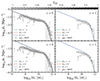 |
Fig. A.1. Stellar mass function for the Planck parameterisation under both Rodriguez-Puebla (top row) and double power-law (bottom row) SMHR. Observational data are provided as a compiled pre-JWST constraints (grey circles) and JWST data (black triangles) |
However, even taking these facts into account, one can notice that for Rodriguez-Puebla SMHR, there is a clear preference for E11≳1, but the dependency of the SMF shape on E22 is extremely weak and subsequently this parameter cannot be effectively constrained, which also applies to the double power-law SMHR. But, for the latter SMHR,E11∼0 is a preferred choice, as E11∼1 overestimates the SMF at higher stellar masses. Notably, the same behaviour can be observed for the z_flex parameterisation (see Figure (A.2)), where gγ cannot be properly constrained, but gμ≳1 is favoured for Model I and gμ∼0 is favoured for Model II SMHR. We note that gμ∼−1 is still allowed by the observational data. On the other hand, the DES parameterisation shows more interesting results, allowing us to constrain both free parameters at low redshifts. Thus, as one can deduce from the Figure (A.3), while working under the Rodriguez-Puebla stellar mass to halo relation, the case of T1∧T2≳1 is strongly preferred. Moreover, for the double power-law SMHR it is unexpected that exactly the opposite applies, i.e. T1∧T2≲−1 is preferred but T2 = 0 is not excluded.
Finally, as the last phenomenological theory we consider the well-known wγCDM with results being displayed in Figure (A.4). Now one can notice the significant deviation at z = 1 from ΛCDM unlike for the previous models. Additionally, Model I SMHR prefers w≳−1.5 while the Model II prefers the range −1≲wΛ<∞ (We note that the evolution of SMF beyond wΛ∼−2 is barely noticeable). The best-fit value of the growth index for the first SMHR appears to be γ≲0.4 while for the Model II it is somewhere in the range of 0.5≲γ≲0.6.
It is important to stress that since the first three phenomenological theories only marginally change the SMF, and therefore best-fit and ΛCDM curves both reside within the uncertainties of the observational data, there is practically no improvement in the statistical sense under the assumption that for example E11≳1 in relation to E11∼0. Subsequently, one can conclude that SMF is a poor probe of phenomenological modified gravity except for wγCDM which can show substantial deviation from ΛCDM at M★≳1010 M⊙.
The results for the first screened case, namely nDGP theory are located in the Figure (A.5). It is interesting to note that at redshifts up to z∼8, Rodriguez-Puebla SMHR prefers rc≳103 Mpc with only lower redshift case allowing for rc≲102.7 Mpc. On the other hand, double power-law SMHR shows strong evidence for rc≳103.5 Mpc at 0<z<4 but can allow for rc∼103 Mpc at the higher redshift range, the beginning of Epoch of Reionisation, i.e. 5<z<8. However, for both kinds of stellar mass to halo relations, the extreme cases of rc≲102.5 Mpc are excluded.
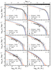 |
Fig. A.5. Stellar mass function for the nDGP gravity under both Rodriguez-Puebla (orange lines) and double power-law (blue lines) SMHR. Observational data are provided as a compiled pre-JWST constraints (grey circles) and JWST data (black triangles) |
On the other hand, let us investigate the more complex k-mouflage model, with the corresponding data being located in the Figures (A.6) and (A.7). At low redshifts under Rodriguez-Puebla SMHR, interestingly the case of β = 0.5 and K0∼1 is preferred over smaller values of free parameters that lead to the ΛCDM-like behaviour. However, at z≥4 the extreme case of β = 0.5 is excluded and from z≥8 onwards even β = 0.3 is excluded as well (vanishing K0 may allow β = 0.3 with tension being <2σ as required, but it can be hypothesised that this will be excluded at even higher redshifts once such data will be made available in the near future). On the contrary, double power-law SMHR shows a strong preference for β = 0.1 on the whole redshift span of our investigation. However, it is important to signify that with β getting smaller, it becomes harder to constrain K0, so in general, for this SMHR, the whole 0<K0<1 range is allowed (potentially, even bigger values can be used without the tension with respect to the observational data being present, but this is beyond the scope of the current study).
As a side note, it is essential to remark that the Rodriguez-Puebla SMHR seems to underestimate SMF at the higher stellar masses even for the ΛCDM, but the double power-law model does not have such a problem, so some parameter constraints that are aimed to fix this issue for the first SMHR may not coincide with the second model (i.e. first model suggests higher deviation from the fiducial cosmology than the second one). Most probably, this issue occurs due to the fact that Rodriguez-Puebla SMHR was calibrated to emulate the high-z observational data rather than low-z.
In addition, double power-law SMHR cannot reproduce the observed slope of the SMF at smaller stellar masses (starting at around M★∼1010 M⊙). The correct slope is reproduced with a higher strength of SN Ia feedback (that suppresses star formation at the lower end of the SMF). Such inconsistency may hint at the fact that the SN Ia feedback calibrated with the help of the UVLF data, rather than SMF/SMD, may incorporate additional yet unknown scatter.
A.2. Constraints from the stellar mass density
The second set of constraints are imposed from the high-redshift observations of the stellar mass density made by JWST, with the results being displayed in the Figures (A.8) and (A.9) respectively. We did not consider phenomenological modifications of gravity such as Planck/DES/wγCDM, as they do not affect high-z structure formation, and thus we only focus our attention on the screened theories.
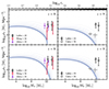 |
Fig. A.8. Stellar mass density for nDGP modified gravity theory versus recent observational data using Rodriguez-Puebla SMHR (upper two subplots) and double power-law SMHR (lower two subplots) |
For the first theory, namely nDGP, there is a significant preference of rc≤103 Mpc, which can be relaxed in the double power-law SMHR case if one will consider higher than fiducial star formation efficiency at the peak mass Mp. However, even for small rc values, Rodriguez-Puebla SMHR could not satisfy SMD constraints completely, as at such high stellar masses M★∼1012 M⊙, star formation is heavily suppressed due to the various feedback mechanisms.
On the other hand, for k-mouflage theory, K0<1 and β≈0.3 was preferred as well as K0≥1 and β≈0.5, but the situation with Rodriguez-Puebla SMHR is similar, while double power-law case can satisfy all of the constraints.
A.3. Constraints from the ultraviolet luminosity function
It is important to denote that unlike the power law SMHR, for the Rodriguez-Puebla one we are going to limit the integration bounds of MUV following the original work (Rodríguez-Puebla et al. 2017), namely at z = 4, the lower bound is MUV=−22.6, at z = 5, MUV=−23, at z = 6, MUV=−22.5, at z = 7, MUV=−22.75 and finally at z = 8, the lower limit is MUV=−22. For other redshifts, we linearly extrapolate the aforementioned limits. Also, in the current work, we are only going to derive the UVLF for two models, namely nDGP and k-mouflage, as any phenomenological model of our consideration will not show noticeable deviation from ΛCDM at z≥4, and there is no UVLF observational data present at smaller redshifts.
We plot the theoretical predictions of UVLF in Figures (A.10) for nDGP gravity and Figures (A.11), (A.12) for k-mouflage. Constraints for each theory here are more uncertain than SMF/SMD as the ultraviolet variance is not as well constrained. However, it can be observed that scatter is around σUV≲1 dex for z≤8 and then it goes up to σUV∼2 dex for z∼12. With the variation of the nDGP free parameter, namely rc, it is possible to adjust the UVLF at brighter magnitudes. Specifically, for both SMHR cases, it can be observed that even if we apply proper σUV kernel, ΛCDM can diverge from the observational data at MUV≲−20, but this can be fixed by setting nDGP parameter to rc≤103 Mpc.
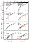 |
Fig. A.10. Ultraviolet luminosity function for the nDGP gravity under both Rodriguez-Puebla (orange lines) and double power-law (blue lines) SMHR. Observational data are provided as a compiled pre-JWST constraints (grey circles) and JWST data (black triangles). Arrows correspond to the upper/lower bounds |
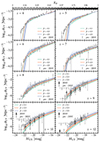 |
Fig. A.11. Figure (A.10) continued, but for the k-mouflage gravity under the Rodriguez-Puebla SMHR |
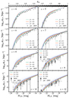 |
Fig. A.12. Figure (A.10) continued, but for the k-mouflage gravity under the double power-law SMHR |
Interestingly enough, k-mouflage theory can satisfy all of the constraints up to z∼12 even with the Gaussian kernel of σUV = 0.4 dex, which is provided by the stellar mass scatter only. Case with β = 0.5, K0∼0.1 has practically perfect correspondence to the observational data for the Rodriguez-Puebla SMHR, but that is only true with z≥8 for the choice of the double power-law.
In general, we have noticed that UVLF is a worse probe of the screened modified gravity in relation to SMF or SMD, as the deviation from ΛCDM caused by the variation of free parameters is a lot less noticeable (especially at the brighter end of the UVLF) while comparing to the SMF. This has also been reported to be the case for other theories in (Schive et al. 2016).
Finally, it is important to signify that double power-law SMHR was not calibrated to work with UVLF in the ΛCDM, and therefore even with proper scatter setup, the results show up to tens of percent of deviation from the observational datasets at lower redshifts.
A.4. Constraints from star formation rate density
The other interesting probe of modified gravity may be the Star Formation Rate Density (SFRD), which is in our case derived from the mass accretion rate paired up with the star formation efficiency. Results for phenomenological theories of modified gravity are shown in Figure (A.13) and for screened theories in the Figure (A.14).
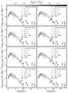 |
Fig. A.13. Star formation rate density for Planck (first row) and z_flex (second row), DES (third row) and wγCDM modified gravity theories. We display results for the Rodriguez-Puebla SMHR in the first column and double power-law SMHR in the second column respectively. Observational data are provided as a compiled pre-JWST constraints (grey circles) and JWST data (black triangles) |
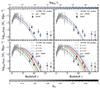 |
Fig. A.14. Figure (A.13) continued, but for nDGP (first row) and k-mouflage (second row) modified gravity theories |
As usual, phenomenological theories show only a very small, in some cases sub-percent deviation from ΛCDM, and some free parameters are impossible to constrain because the variation of the letter is smaller than the uncertainties in the SFRD measurements. However, we can still see that E11≳1, gμ≳1 and T1∧T2≳1 are preferred choices. On the other hand, wγCDM gives more significant deviation from the fiducial cosmology, and for low-z SFRD constraints to be satisfied, wΛ≤−1, which makes phantom cosmology a viable choice.
Screened theories are far easier to constrain. As an example, at rc≤103 Mpc, nDGP theory shows underwhelming SFRD prediction at lower redshifts but in turn, satisfies high-z JWST data and vice-versa (which is true for both SMHR choices). In contrast, k-mouflage can satisfy both high and low redshift constraints up to z∼12 if one will take β∼0.3 and K0∼0.5 (which seems to be the only possible choice, as β = 0.1 has smaller than expected SFRD at high redshifts and β = 0.5 at low redshifts respectively), while working under the Rodriguez-Puebla SMHR and β≲0.1, K0∼1 under double power-law SMHR. It is evident that for both nDGP and k-mouflage models, for any choice of free parameters, there is still a minor inconsistency between theoretical and observational data at small redshifts. This phenomenon was previously found in the literature, for example in EAGLE simulation output (Furlong et al. 2015), Horizon Run 5 simulation output (Lee et al. 2021) and Illustris-TNG simulation output (Pakmor et al. 2023) respectively. The solution was to introduce an additional scatter of 0.2 dex, which presumably arises due to some, yet unknown star formation mechanisms. Such scatter can also help satisfy higher redshift constraints imposed by JWST and allow the case of β = 0.1, decreasing the departure from ΛCDM for k-mouflage theory. Interestingly, a scatter of only 0.05 dex or even less (depending on the value of a free parameter) is required for the double power law model. For any model and any scatter value, it is still not possible to produce the nearly constant SFRD, required by JWST at z≳12. In (Harikane et al. 2023), it was also noted that SFRD at such redshifts cannot be reproduced with the constant SFE models. Unlike the lower redshift measurements of SFRD, JWST measurements rely on the photometric redshifts. Also, the sample size is small and its robustness may change the observed SFRD by up to an order of magnitude (Bouwens et al. 2023a).
Thus, Rodriguez-Puebla SMHR can very precisely reconstruct the SMF and SMD, but cannot reconstruct SFRD without the introduction of additional scatter. The opposite is true for the double power law. Such inconsistencies between SMF/SMD and SFRD have been noticed before on the whole 0<z<8 range and are explored further in the work of Yu & Wang (2016). The main issue is that Rodriguez-Puebla SMHR is calibrated on the basis of SMF and SMD observational data, but double power law SMHR rather uses UVLF. Since the connection between UV magnitude and halo mass is subject to a scatter that is yet to be properly determined, each model cannot satisfy all of the constraints imposed.
A.5. Constraints from Epoch of Reionisation
The final set of constraints comes from the epoch of reionisation, namely ionised hydrogen volume filling fraction QHII and optical depth τ. Similarly to the UVLF and SMD cases, we do not consider phenomenological modifications of gravity in this section, as reionisation happens when dark energy mass density is practically negligible and thus will have no effect on QHII or τ. The optical depth is integrated from the present time until the end of reionisation, so it captures the dark energy dominated epoch. However, during that epoch, QHII∼1, and thus the effect of the phenomenological modified gravity on the optical depth is also negligible.
The volume filling fraction and the optical depth for screened theories are shown in Figure (A.15). We first consider the nDGP gravity. We note that under the Rodriguez-Puebla SMHR, the volume filling fraction of the ionised hydrogen predicted by nDGP cannot satisfy observational constraints for any value of rc and in general, the variation of QHII(z) with rc is only marginal. On the other hand, observational constraints for the double power-law SMHR are satisfied for the whole range rc≳103 Mpc.
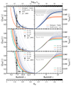 |
Fig. A.15. Volume filling fraction of HII (left column) and optical depth (right column) for nDGP (first row), k-mouflage Rodriguez-Puebla (second row) and double power-law SMHR (third row). Observational constraint on the optical depth by the Planck probe is provided as a grey band |
Under the condition that rc≲102.7 Mpc, the predicted optical depth for both SMHRs is higher than the one of Planck2018 measurement, but consistent with the reionisation history based on the JWST-calibrated Nion value (Muñoz et al. 2024). On the other hand, Planck data implies that 102.7 Mpc≲rc≲103 Mpc for Rodriguez-Puebla and that rc≳103 Mpc for double power-law SMHR respectively.
The other model, k-mouflage, was able to satisfy reionisation constraints for both SMHRs. Under the assumptions of a Rodriguez-Puebla SMHR, the preferred values are β∼0.3 and K0≳0.5 or β∼0.5 and K0∼1. Besides, given double power-law SMHR, the only plausible choice is that β≲0.1 and K0∼1.
One thing that we should denote is that we are using the star formation rate density already with the suitable scatter introduced (0.2 dex in the case of Rodriguez-Puebla and 0.05 dex in the case of double power-law SMHR respectively). Without this scatter, the reionisation should occur later.
All Figures
|
Fig. 1. Structure of this paper. |
| In the text | |
|
Fig. 2. Matter power spectrum predictions for phenomenological modified gravity versus observational data with varying values of E11, E22 (first subplot), gμ, and gγ, constant n = 1 (second subplot); for varying values of T1=T3 and T2=T4, constant n = 1 (third subplot); a running growth index γ; and dark energy EoS wΛ (fourth subplot). |
| In the text | |
|
Fig. 3. Same as Figure 2 but for the nDGP gravity with varying rc (first subplot) and k-mouflage gravity with varying β, K0 (second subplot). |
| In the text | |
|
Fig. 4. Linear density contrast for the spherical collapse occurring at the time ac within DES, z_flex, and Taylor expanded DES, varying wΛ and γ phenomenological theories of gravitation. |
| In the text | |
|
Fig. 5. Linear density contrast for the spherical collapse occurring at the time ac within screened MOG models, namely nDGP and k-mouflage. |
| In the text | |
|
Fig. 6. Virial overdensity for phenomenological models. |
| In the text | |
|
Fig. 7. Virial overdensity for the theories of modified gravitation with the screening field present, namely, nDGP and k-mouflage. |
| In the text | |
|
Fig. 8. Compilation of the best-fit parameters determined by the visual inspection of various observables for nDGP (first column) and k-mouflage (second and third columns). Arrows signify an upper limit for a parameter, while shaded areas represent the parameter space preferred by the vast majority of observational datasets. |
| In the text | |
|
Fig. A.1. Stellar mass function for the Planck parameterisation under both Rodriguez-Puebla (top row) and double power-law (bottom row) SMHR. Observational data are provided as a compiled pre-JWST constraints (grey circles) and JWST data (black triangles) |
| In the text | |
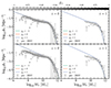 |
Fig. A.2. Figure (A.1) continued, but for the z_flex parameterisation |
| In the text | |
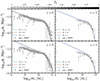 |
Fig. A.3. Figure (A.1) continued, but for the DES parameterisation |
| In the text | |
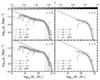 |
Fig. A.4. Figure (A.1) continued, but for the wγCDM modified gravity |
| In the text | |
|
Fig. A.5. Stellar mass function for the nDGP gravity under both Rodriguez-Puebla (orange lines) and double power-law (blue lines) SMHR. Observational data are provided as a compiled pre-JWST constraints (grey circles) and JWST data (black triangles) |
| In the text | |
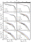 |
Fig. A.6. Figure (A.5) continued, but for the k-mouflage gravity under the Rodriguez-Puebla SMHR |
| In the text | |
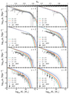 |
Fig. A.7. Figure (A.5) continued, but for the k-mouflage gravity under the double power-law SMHR |
| In the text | |
|
Fig. A.8. Stellar mass density for nDGP modified gravity theory versus recent observational data using Rodriguez-Puebla SMHR (upper two subplots) and double power-law SMHR (lower two subplots) |
| In the text | |
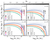 |
Fig. A.9. Figure (A.8) continued, but for the k-mouflage gravity |
| In the text | |
|
Fig. A.10. Ultraviolet luminosity function for the nDGP gravity under both Rodriguez-Puebla (orange lines) and double power-law (blue lines) SMHR. Observational data are provided as a compiled pre-JWST constraints (grey circles) and JWST data (black triangles). Arrows correspond to the upper/lower bounds |
| In the text | |
|
Fig. A.11. Figure (A.10) continued, but for the k-mouflage gravity under the Rodriguez-Puebla SMHR |
| In the text | |
|
Fig. A.12. Figure (A.10) continued, but for the k-mouflage gravity under the double power-law SMHR |
| In the text | |
|
Fig. A.13. Star formation rate density for Planck (first row) and z_flex (second row), DES (third row) and wγCDM modified gravity theories. We display results for the Rodriguez-Puebla SMHR in the first column and double power-law SMHR in the second column respectively. Observational data are provided as a compiled pre-JWST constraints (grey circles) and JWST data (black triangles) |
| In the text | |
|
Fig. A.14. Figure (A.13) continued, but for nDGP (first row) and k-mouflage (second row) modified gravity theories |
| In the text | |
|
Fig. A.15. Volume filling fraction of HII (left column) and optical depth (right column) for nDGP (first row), k-mouflage Rodriguez-Puebla (second row) and double power-law SMHR (third row). Observational constraint on the optical depth by the Planck probe is provided as a grey band |
| In the text | |
Current usage metrics show cumulative count of Article Views (full-text article views including HTML views, PDF and ePub downloads, according to the available data) and Abstracts Views on Vision4Press platform.
Data correspond to usage on the plateform after 2015. The current usage metrics is available 48-96 hours after online publication and is updated daily on week days.
Initial download of the metrics may take a while.