| Issue |
A&A
Volume 689, September 2024
|
|
|---|---|---|
| Article Number | A39 | |
| Number of page(s) | 12 | |
| Section | Cosmology (including clusters of galaxies) | |
| DOI | https://doi.org/10.1051/0004-6361/202450050 | |
| Published online | 02 September 2024 | |
A simple prediction of the nonlinear matter power spectrum in Brans–Dicke gravity from linear theory
Institute of Theoretical Astrophysics, University of Oslo, PO Box 1029 Blindern, 0315 Oslo, Norway
Received:
20
March
2024
Accepted:
29
May
2024
Abstract
Brans–Dicke (BD), one of the first proposed scalar-tensor theories of gravity, effectively makes the gravitational constant of general relativity (GR) time-dependent. Constraints on the BD parameter ω serve as a benchmark for testing GR, which is recovered in the limit ω → ∞. Current small-scale astrophysical constraints ω ≳ 105 are much tighter than large-scale cosmological constraints ω ≳ 103, but the two decouple if the true theory of gravity features screening. On the largest cosmological scales, BD approximates the most general second-order scalar–tensor (Horndeski) theory, so constraints here have wider implications. These constraints will improve with upcoming large-scale structure and cosmic microwave background surveys. To constrain BD with weak gravitational lensing, one needs its nonlinear matter power spectrum PBD. By comparing the boost B = PBD/PGR from linear theory and nonlinear N-body simulations, we show that the nonlinear boost can simply be predicted from linear theory if the BD and GR universes are parameterized in a way that makes their early cosmological evolution and quasilinear power today similar. In particular, they need the same H0/√Geff(a = 0) and σ8, where Geff is the (effective) gravitational strength. Our prediction is 1% accurate for ω ≥ 100, z ≤ 3, and k ≤ 1 h/Mpc; and 2% up to k ≤ 5 h/Mpc. It also holds for GBD that do not match Newton’s constant today, so one can study GR with different gravitational constants GGR by sending ω → ∞. We provide a code that computes B with the linear Einstein-Boltzmann solver HI_CLASS and multiplies it by the nonlinear PGR from EUCLIDEMULATOR2 to predict PBD.
Key words: methods: numerical / cosmological parameters / large-scale structure of Universe
Corresponding author; This email address is being protected from spambots. You need JavaScript enabled to view it. .
© The Authors 2024
 Open Access article, published by EDP Sciences, under the terms of the Creative Commons Attribution License (https://creativecommons.org/licenses/by/4.0), which permits unrestricted use, distribution, and reproduction in any medium, provided the original work is properly cited.
This article is published in open access under the Subscribe to Open model. This email address is being protected from spambots. You need JavaScript enabled to view it. to support open access publication.
1. Introduction
The Brans–Dicke (BD) theory (Brans & Dicke 1961; Dicke 1962) of modified gravity (MG; Clifton et al. 2012) features a scalar field in addition to the spacetime metric. It effectively promotes Newton’s constant in general relativity (GR) to a dynamical gravitational strength. This scalar–tensor theory was introduced in the 1960s to implement Mach’s principle in GR. Since then it has become perhaps the most famous alternative to Einstein’s theory and a root for the development of other theories, such as the more general Horndeski theory (Horndeski 1974). BD features an additional parameter ω and reduces to GR as ω → ∞, so BD can be understood as a generalization of GR. In cosmology, replacing GR with BD in the standard Λ cold dark matter ((GR-)ΛCDM) model gives the alternative BD-ΛCDM model, where the effective gravitational strength evolves with time and modifies the expansion history and growth of structure.
As summarized in Table 1, observations in the 21st century have placed very strong constraints on ω. Already in 2003, Shapiro time delay measurements of the Cassini satellite on its way to Saturn constrained ω ≳ 104, and recent strong-field tests from timing rapidly rotating neutron stars (pulsars) even bound ω ≳ 105. On cosmological scales, however, the story is different. Roughly speaking, constraints have tightened from only ω ≳ 102 with stage-II survey data in the 2000s to ω ≳ 103 with stage-III surveys in the 2010s. In the next decade, Alonso et al. (2017) expects cosmological constraints to improve by another order of magnitude with upcoming stage-IV surveys like Euclid (Laureijs et al. 2011), DESI (DESI Collaboration 2016), the Vera C. Rubin Observatory (LSST Science Collaboration 2009), SKA (Yahya et al. 2015) and next-generation cosmic microwave background (CMB) experiments (Abazajian et al. 2016). Fisher forecasts found that if ω = 800, then Euclid should be able to constrain this to 3% using galaxy clustering and weak lensing data (Frusciante et al. 2024). Likewise, Ballardini et al. (2019) forecast that upcoming clustering and weak lensing data in combination with BOSS and CMB observations have the potential to reach ω ≳ 104 in the most optimistic case. With these seemingly ever-tightening competing constraints, BD has become a benchmark theory for testing (deviations from) GR. BD also survived the burial of theories with gravitational wave speeds v ≠ c from GW170817 (Ezquiaga & Zumalacárregui 2017), and Solà Peracaula et al. (2019, 2020) show that it alleviates the H0 and S8 tensions (Perivolaropoulos & Skara 2022).
Constraints on the BD parameter ω from various tests, beginning with the Cassini bound from 2003.
In fact, several scalar–tensor theories reduce to BD on large (cosmological) scales, where gradients of the scalar field are suppressed (Avilez & Skordis 2014; Joudaki et al. 2022). This makes BD interesting not only on its own, but also as the large-scale limit of more general theories, so constraints on it have wider implications. Such theories typically feature screening mechanisms that hide the scalar field in dense small-scale regions, letting GR take over there. In other words, the true theory of gravity could be similar to BD on the largest scales, similar to GR on the smallest scales, and transition between them over intermediate scales. The very tight small-scale (astrophysical) constraints could therefore be irrelevant from a cosmological perspective.
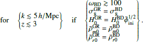
In this work, we aim to develop a tool for predicting the nonlinear BD-ΛCDM matter power spectrum PBD(k ≲ 5 h/Mpc, z ≲ 3 | θ) across parameter space θ to around 1% precision, for use in constraining the theory with upcoming stage-IV large-scale structure survey data. There are several possible approaches to this, all of which rely on N-body simulations to account for the nonlinear evolution.
Halo modeling tools like HMCODE (Mead et al. 2015, 2021) and HALOFIT (Smith et al. 2003; Takahashi et al. 2012) rely on dark matter’s clustering in halos to effectively reverse-engineer the nonlinear matter distribution from halo statistics. They can be integrated directly with linear Einstein-Boltzmann solvers. The HMCODE framework has been extended to account for a wide range of dark energy and MG models, massive neutrinos and baryonic physics (Mead et al. 2016). Another related method is the halo model reaction approach of Cataneo et al. (2019), which combines the halo model and perturbation theory to model corrections coming from nonstandard physics. This is implemented in the publicly available REACT code (Bose et al. 2020; Giblin et al. 2019). The halo modeling approach was taken in Joudaki et al. (2022), who used N-body simulations to create a fitting formula in HMCODE to predict the nonlinear BD-ΛCDM power spectrum. As far as we know, this is the only nonlinear prediction for BD so far.
Emulators are trained from a set of (time-consuming) N-body simulations for a limited number of cosmological parameters, and then rely on machine learning to (quickly) interpolate in parameter space and output the nonlinear matter power spectrum for arbitrary cosmologies. There are already sophisticated emulators for the GR-ΛCDM power spectrum, such as EUCLIDEMULATOR2 (Euclid Collaboration 2021), COSMICEMU (Heitmann et al. 2016; Lawrence et al. 2017; Moran et al. 2023), and BACCO (Angulo et al. 2021; Aricò et al. 2021, 2022). Recent works, including Winther et al. (2019), Brando et al. (2022), Fiorini et al. (2023), SESAME (Mauland et al. 2024), and E-MANTIS (Sáez-Casares et al. 2024), have produced emulators for selected MG theories. It is also possible to combine halo modeling with emulation and emulate the ingredients of the halo model (Ruan et al. 2024). At the time of writing, no dedicated BD-ΛCDM power spectrum emulator exists.
Simulation rescaling (Angulo & White 2010) is a technique where data from a single N-body simulation is rescaled to produce output for a different cosmology. This technique was in fact used in training the BACCO emulator.
We demonstrate a hybrid technique, somewhat reminiscent of both rescaling and emulation, suited to extending existing predictors of GR-ΛCDM to BD-ΛCDM. By carefully selecting the cosmological parameters θBD and θGR, we map a given BD universe to a corresponding GR universe such that their cosmological evolutions are as similar as possible. This makes it possible to predict the nonlinear matter power spectrum boost 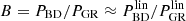 using linear power spectra from cheap Einstein-Boltzmann solvers, which we verified by comparing it to the boost obtained from N-body simulations. In turn, we can predict the full BD-ΛCDM power spectrum PBD = B ⋅ PGR by combining it with any existing high-quality emulator for PGR. This “trick” exploits the effort that has already gone into creating sophisticated GR emulators, and avoids duplicating this work for every alternative model to be explored. It could be a viable cheap route for constraining MG theories with upcoming surveys (Frusciante et al. 2024; Casas et al. 2017).
The rest of this paper is structured as follows. Section 2 reviews the background cosmology and perturbation theory of BD (and thus GR). Section 3 describes our pipeline for the Einstein-Boltzmann solver and N-body simulations. Section 4 justifies the parameterization we use to compute the boost. Section 5 shows the resulting linear and nonlinear boost and compares them to older predictions. Section 6 concludes.
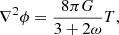
2. Brans–Dicke modified gravity
Brans–Dicke (BD) theory (Brans & Dicke 1961; Dicke 1962) generalizes general relativity (GR). In addition to the metric tensor gμν, it features a scalar field ϕ with a constant dimensionless parameter ω. Here we use units where c = 1, but explicitly keep Newton’s constant G = 6.67 × 10⁻¹¹ Nm2/kg2 to show how BD effectively modifies the gravitational constant of GR. In the Jordan frame, the total action of BD gravity minimally coupled to the matter action SM is
![Mathematical equation: $$ \begin{aligned} S\left[g_{\mu \nu },\phi \right] = \frac{1}{16 \pi G} \int \mathrm{d}^4 x \sqrt{-|g|} \, \bigg [ \phi R - \frac{\omega }{\phi } (\nabla \phi )^2 \bigg ] + S_{\rm M}, \end{aligned} $$](/articles/aa/full_html/2024/09/aa50050-24/aa50050-24-eq3.gif) (1)
(1)
where gμν is the spacetime metric with determinant |g|< 0, Ricci scalar R and covariant derivative ∇μ; and (∇ϕ)2 = (∇μϕ)(∇μϕ) = gμν(∇μϕ)(∇νϕ). From the principle of least action δS = 0, the (classical) equations of motion for gμν and ϕ are the modified Einstein and Klein-Gordon field equations (Clifton et al. 2012)
![Mathematical equation: $$ \begin{aligned} G_{\mu \nu }&= \frac{8 \pi G}{\phi } T_{\mu \nu } + \frac{\omega }{\phi ^2} \bigg [ (\nabla _\mu \phi ) (\nabla _\nu \phi ) - \frac{1}{2} g_{\mu \nu } (\nabla \phi )^2 \bigg ] \nonumber \\ &\quad + \frac{1}{\phi } \bigg [ \nabla _\mu \nabla _\nu \phi - g_{\mu \nu } \nabla ^2 \phi \bigg ], \end{aligned} $$](/articles/aa/full_html/2024/09/aa50050-24/aa50050-24-eq4.gif) (2a)
(2a)
 (2b)
(2b)
where ∇2 = gμν∇μ∇ν is the four-dimensional Laplacian, and  is the energy-momentum tensor of matter with trace
  . Effectively, ϕ promotes Newton’s constant G in the Einstein field equations (2a) to a dynamical field G/ϕ. In the following, we see in more detail how BD is similar to GR with such an effective gravitational strength.
GR is recovered in the limit ω → ∞: then ∇2ϕ = 0, whose solution ϕ = 1 everywhere recovers Einstein’s field equations Gμν = 8πG Tμν with Newton’s constant G.
2.1. Cosmology
We assume a spatially flat, homogeneous and isotropic Friedmann–Lemaître–Robertson–Walker background with small perturbations in the Newtonian gauge:
![Mathematical equation: $$ \begin{aligned} \mathrm{d}s^2 = -\big [1+2\Psi (t,\boldsymbol{x})\big ] \mathrm{d}t^2 + a^2(t) \big [1+2\Phi (t,\boldsymbol{x})\big ] \mathrm{d}\boldsymbol{x}^2. \end{aligned} $$](/articles/aa/full_html/2024/09/aa50050-24/aa50050-24-eq8.gif) (3)
(3)
We fill the universe with a perfect fluid with total energy-momentum tensor
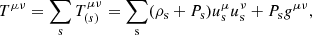 (4)
(4)
with energy densities ρs, pressures Ps, and four-velocities  from the species s:
-
radiation r (from photons γ and massless1 neutrinos ν) with equation of state
 ,
, -
matter m (from baryons b and cold dark matter c) with equation of state
 ,
, -
dark energy Λ (from a cosmological constant) with equation of state
 .
.
The universe’s background and (linear) perturbations are described perturbatively up to first order around a homogeneous and isotropic universe.
2.2. Background cosmology
To zeroth order, the equation of motions (2) give the Friedmann and scalar field equations
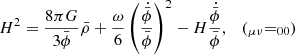 (5a)
(5a)
 (5b)
(5b)
where 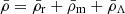 ,
,  , ˙ = d/dt and H = ȧ/a is the Hubble parameter. The Friedmann equation in BD is the same as in GR, only with additional effective energy from
  and an effective gravitational strength
  .
.
According to the Boltzmann equation, the three species evolve as  ,
,  and
and  , where 0 indexes quantities by their values today. Defining the standard density parameters
  , physical densities today are measured by
 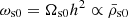 2. Re-parameterizing the evolution in terms of ′=d/dlna = H−1 ⋅ d/dt, the system (5) can be rewritten in the dimensionless form
![Mathematical equation: $$ \begin{aligned} E^2 = \left(\frac{H}{H_0}\right)^2&= \frac{1}{\bar{\phi }} \cdot \frac{\displaystyle \Omega _{\rm r0} a^{-4} + \Omega _{\rm m0} a^{-3} + \Omega _{\Lambda 0}}{1 - \frac{\omega }{6} [(\ln \bar{\phi })^\prime ]^2 + (\ln \bar{\phi })^\prime }, \end{aligned} $$](/articles/aa/full_html/2024/09/aa50050-24/aa50050-24-eq25.gif) (6a)
(6a)
 (6b)
(6b)
This system can be integrated from an initial scale factor aini, given  ,
,  , Ωr0, Ωm0, ΩΛ0, and ω. But these are not all free parameters, as today’s Friedmann equation E0 = 1 constrains one of them – say ΩΛ0. To find a consistent solution, one can iterate over ΩΛ0 and solve the system repeatedly until this constraint is satisfied.
The integration can be simplified by selecting aini in the radiation era. There H ∝ a−2 and 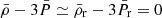 , so the Klein–Gordon equation (5b) gives
  with the solution
  . The diverging solution is unphysical, leaving a frozen
  with
with
 (7)
(7)
In the Poisson equation (9) below, we see that the effective gravitational strength felt by matter today depends on ω and  . We therefore used the shooting method to vary
  and integrate the system repeatedly until we hit the desired
  .
.
2.3. Linear perturbations
Ignoring anisotropic relativistic stresses and polarization and working in the quasi-static limit  and sub-horizon limit k ≫ H (Orjuela-Quintana & Nesseris 2023), the linearly perturbed Boltzmann, Einstein and Klein–Gordon equations in k-space are (Solà Peracaula et al. 2019)
 (8a)
(8a)
 (8b)
(8b)
 (8c)
(8c)
 (8d)
(8d)
 (8e)
(8e)
 (8f)
(8f)
 (8g)
(8g)
 (8h)
(8h)
 (8i)
(8i)
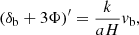
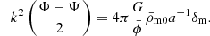
Motion of matter is sensitive to Ψ through the geodesic equation. In matter domination, δP ≃ 0 and  , and solving equations (8g), (8h) and (8i) for Ψ gives its Poisson equation
 (9)
(9)
The Poisson equation in BD is the same as in GR, only with an effective gravitational strength  felt by matter that depends on time through the scalar field in the background. Cavendish experiments today measure Gm0, so the scalar field today must be
  in “restricted models” with the correct Newtonian limit Gm0 = G. However, we also allowed for “unrestricted models” with arbitrary Gm0 and
  , so we can constrain Gm0 with cosmology (Zahn & Zaldarriaga 2003; Ballardini et al. 2022).
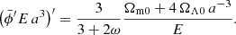
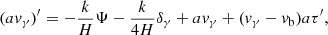
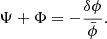
To find a simplified growth equation for the total matter overdensity δm, baryon–photon interactions at late times can be neglected. Combining the Boltzmann equations (8a), (8b), (8d) and (8e) with the Poisson equation (9) then gives the growth equation
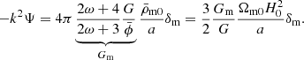
![Mathematical equation: $$ \begin{aligned} 0&= \ddot{\delta }_{\rm m} + 2H\dot{\delta }_{\rm m} - 4 \pi G_{\rm m} \bar{\rho }_{\rm m} \delta _{\rm m} \nonumber \\&= H^2 \bigg \{ \delta _{\rm m}^{\prime \prime } + \Big [ 2 + (\ln E)^\prime \Big ] \delta _{\rm m}^\prime - \frac{3}{2} \frac{G_{\rm m}}{G} \Omega _{\rm m}(a) \delta _{\rm m} \bigg \}. \end{aligned} $$](/articles/aa/full_html/2024/09/aa50050-24/aa50050-24-eq52.gif) (10)
(10)
The general solution of this second-order differential equation is a linear combination δm(k, a) = C+(k)D+(a)+C−(k)D−(a) of a growing mode D+(a) and a decaying mode D−(a). The growing mode is called the scale-independent growth factor D+(a), and, neglecting the decaying mode, relates D+(a2)/D+(a1) = δm(k, a2)/δm(k, a1) for any k.
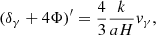
On the other hand, deflection of light through weak lensing is sensitive to the Weyl potential (Ψ − Φ)/2. To find its source equation, eliminate δϕ from equations (8g), (8h), and (8i) to get
 (11)
(11)
Here we see that it is the effective  that affects light trajectories. In general, we encountered three effective gravitational strengths Gγ = GH ≠ Gm that affect light trajectories, the expansion and matter clustering, respectively. Although they generally take on two different values, we have Gγ = GH ≈ Gm for (viable) models with appreciable ω.
The growth of structure is summarized by the matter power spectrum
 (12a)
(12a)
of the gauge-invariant density perturbation Δm ≈ δm amplified from a nearly scale-invariant (ns ≲ 1) primordial power spectrum
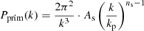 (12b)
(12b)
with primordial amplitude As and spectral index ns.
2.4. Nonlinear structure formation
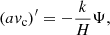
To perform N-body simulations in BD we only need the geodesic equation
 (13)
(13)
and the Poisson equation
 (14)
(14)
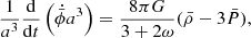
The geodesic equation is the same in BD and GR, and the Poisson equation is the same as the linear version (9). The only two modifications from a GR N-body simulation are the modified Hubble function H(a) and the effective gravitational strength Gm(a), making it trivial to extend any N-body code from GR to BD.
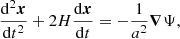
Figure 1 compares the background evolution in two BD-ΛCDM and GR-ΛCDM universes with cosmological parameters to be introduced in Sect. 4 and Table 2.
 |
Fig. 1. Evolution of the effective gravitational parameter G, Hubble function E(a) = H(a)/H0, growth factor D(a), and growth rate f(a) = d lnD(a)/d lna from equations (5) and (10) with the scale factor a in the fiducial BD-ΛCDM and GR-ΛCDM cosmologies in Table 2 (equivalent to the transformation in Fig. 5a). The common time of matter-radiation equality is marked by |

Independent cosmological parameters θ for BD-ΛCDM and GR-ΛCDM and, their fiducial values.
3. Computational pipeline
To compute the matter power spectrum P(k, z | θ) in a BD-ΛCDM or GR-ΛCDM universe, we joined three codes into the pipeline in Fig. 2:
-
HI_CLASS (Zumalacárregui et al. 2017; Bellini et al. 2020), based on CLASS (Blas et al. 2011), solves the background and perturbation Einstein-Boltzmann equations in GR-ΛCDM and several MG cosmologies, including BD-ΛCDM. The perturbed equations it solves are more sophisticated than our simplified presentation (8) and too lengthy to reproduce here. It outputs the linear matter power spectrum PHI_CLASS(k,z). Bellini et al. (2018) showed that its BD matter power spectrum agrees to 0.1% with four other codes.
-
FML3 is a particle-mesh N-body code that uses the COLA method (Tassev et al. 2013) in GR-ΛCDM and several MG cosmologies, including BD-ΛCDM. It supersedes the code MG-PICOLA (Winther et al. 2017), in turn based on L-PICOLA (Howlett et al. 2015). The code first backscales the linear power spectrum (see e.g. Fidler et al. (2017)) from HI_CLASS, and then seeds initial particle positions. It then solves the Poisson equation (14) with the time-dependent Gm(t) in BD and Newton’s constant Gm = G in GR, Finally, it outputs the (quasi-)nonlinear matter power spectrum PCOLA(k, z) by constructing the density field from the particle position snapshots. These results are used for our main analysis. We used a box with volume L3 = (384 h/Mpc)3 and Npart = Ncell = 5123 particles and cells, evolving from redshift zinit = 10 until today with Nstep = 30 time steps. These simulations sacrifice accuracy at the deepest nonlinear scales for overall computational speed: the particle-mesh nature of the code does not resolve small-scale forces, and the COLA method maintains accuracy up to quasilinear scales with few time steps. This is an excellent trade-off in our scenario. To some extent, the error in P at smaller scales even cancels after we compute the boost PBD/PGR.
-
RAMSES (Teyssier 2002) solves the Poisson equation with the standard N-body method with adaptive mesh refinement and time-stepping in GR-ΛCDM and (with our modifications) BD-ΛCDM. We modified its GR version4 to solve the same Poisson equation as FML using arbitrary splined functions for H(a) and Gm(a) over time, passed on from HI_CLASS. It starts from the same initial particle positions at the same redshift zinit as FML, uses the same box size L and number of particles Npart, adaptively refines a base grid with the same size Ncell, but uses adaptive time stepping that ignores FML’s Nstep. The snapshots are analyzed in the same way as FML, except that we quadrupled the number of grid cells along each dimension due to the finer resolution. This also outputs the nonlinear matter power spectrum PRAMSES(k,z), and is only used to validate FML’s results.
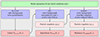 |
Fig. 2. Our BD- or GR-specific simulation pipeline begins from a set of input parameters θBD or θGR. First, they are passed to the Einstein-Boltzmann solver HI_CLASS, which solves the background and perturbations and outputs the linear power spectrum. Next, FML back-scales PHI_CLASS(k,z) from z = 0 to z = zinit, realizes initial conditions for an N-body simulation with the random seed s and evolves it forward with the COLA method on a uniform grid, outputting the nonlinear power spectrum. Finally, FML’s first snapshot can be passed on to RAMSES, which evolves the same initial conditions with the standard N-body method on an adaptive mesh and yields an independent nonlinear power spectrum. |
All codes branch to solve the equations specific to BD-ΛCDM or GR-ΛCDM at all times. To compensate for slight code differences, such as time stepping and splining effects, we normalized P from FML and RAMSES to match that from HI_CLASS at the most linear common scale k = 0.02 h/Mpc.
3.1. Boost computation
To compute the matter power spectrum boost
 (15)
(15)
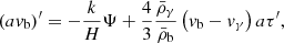
our pipeline first runs one BD simulation with freely chosen parameters θBD, followed by one GR simulation with parameters θGR = θGR(θBD) decided by a transformation of the BD parameters. It then compares the power spectra at equal redshifts z, but generally different wavenumbers kBD and kGR = kGR(kBD), which we justify in Sect. 4.
To minimize cosmic variance within each (BD, GR) simulation pair, it uses a common initial condition seed sBD = sGR = s (for fixed θBD and θGR). But the seed s = s(θBD) is changed for every new set of parameters to avoid bias toward one particular configuration of the universe. To further reduce cosmic variance, we also used amplitude-fixed initial conditions (Angulo & Pontzen 2016; Villaescusa-Navarro et al. 2018).
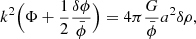
3.2. Tests and convergence analysis
HI_CLASS and FML independently calculate E(a) = H(a)/H0, ΩΛ0, and σ8 in GR, and also  and
and  in BD. We verified that these agree within a small tolerance after every run.
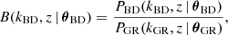
Figure 3 shows a convergence analysis of the results from FML. The results change by less than 1% when the increasing the resolution of the simulation parameters, showing that the results from our setup have converged.
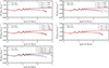 |
Fig. 3. Convergence of FML’s boost (15) at z = 0 in the fiducial cosmology in Table 2 (equivalent to the transformation in Fig. 5a), as computational parameters are varied from the fiducial Npart = 5123, Ncell = 5123, Nstep = 30, zinit = 10, and L = 384 Mpc/h. |
To test the absolute accuracy of the particle-mesh simulations we ran using FML, we also compared it to results from the adaptive-mesh-refinement code RAMSES. These results are shown in Fig. 4 and again, the results are equal up to 1% error up to k ≲ 5 h/Mpc. Together, these tests show that the results of the boost from FML are both precise and accurate to 1% error. We only performed these tests for the fiducial cosmology in Table 2: we chose a small value ω = 100 in BD to maximize the deviation from GR, and assume the results can be trusted for other cosmological parameters.
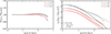 |
Fig. 4. Comparison of the matter power spectrum (boost) obtained from FML using the COLA method on a uniform grid and RAMSES using the standard N-body method on an adaptive grid, in the fiducial cosmology in Table 2 (equivalent to the transformation in Fig. 5a). To compensate for small code differences, we have rescaled all spectra to match the linear HI_CLASS spectrum at their smallest common k. We cut RAMSES’ spectra at increasingly higher k ≤ {1/2, 1, 2}⋅kNyquist as the mesh refinement increases for z = {3, 1.5, 0}. Although P from FML and RAMSES disagree, that error largely cancels in their boosts B = PBD/PGR, which agree to 1% up to k ≲ 5 h/Mpc. |
4. Model parameterization
What parameter and wavenumber transformations θGR(θBD) and kGR(kBD) should we use in the boost (15)? That is, how should we compare a BD universe to a GR universe? The answer may sound as obvious as the question sounds pedantic: that we should use the same parameters in BD and GR. But this is vague or impossible, as it depends on our selection of cosmological parameters, and all cosmological parameters cannot be equal in two different universes. For example, the background equations (5) forbid having the same  ,
,  ,
,  , H0 and
  today. For us this is a question of convenience. We can choose to compare two universes in the boost (15) such that this ratio behaves as simple and predictable as possible. At the end of the day, we want to multiply it by PGR to predict PBD, anyway.
Next, we discuss some transformation alternatives while testing them in Fig. 5.
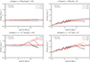 |
Fig. 5. Matter power spectrum boost (15) with different parameter transformations θGR = θGR(θBD), where ( |


4.1. Wavenumbers and Hubble parameter
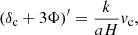
Consider the perturbations (8) and forget about recombination for a moment, which enters through the optical depth τ. In the Boltzmann equations, k and H appear in the particular combination k/H. At early times, the same is true for the Einstein and Klein-Gordon equations after substituting the effective  from the Friedmann equation (5a) with the frozen scalar field (7). For large enough ω that sufficiently suppress the anisotropic stress
  , perturbations in BD and GR with equal k/H (or
  ) evolve similarly.
In other words, BD resembles GR with a different expansion rate H due to a different effective gravitational strength. This difference can be factored out by comparing modes with equal k/H (or  ). Similarly, (Zahn & Zaldarriaga 2003, equation (12)) shows that a mode k′ in a GR universe with gravitational constant G′ evolves like a mode
  in another GR universe with Newton’s constant G. In other words, as they elegantly explained it, “gravity introduces no preferred scale, so the dynamics of the perturbations remains the same when scales are measured in units of the expansion time.” This also holds for BD’s scale-independent effective gravitational strength.
However, it breaks when recombination is activated and τ is included, as the faster expansion hinders (re)combination of H+ + e− and dampens the small-scale acoustic peaks in the CMB spectrum. This is indeed how Zahn & Zaldarriaga (2003) shows how the CMB constrains G to percent-level. However, most matter is dark, so this effect is much smaller for the power spectrum of matter that concerns us here.
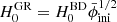
This motivates matching modes {kBD, kGR} such that k/H is the same at early times. To be compatible with N-body codes that factor H0 out of the relevant equations, we can compare modes with equal k/H0 as long as we make EBD = EGR at early times. The frozen scalar field (7) cuts the Friedmann equation (5a) off at  provided we use the same physical densities
  in BD and GR5 so we can accomplish this by transforming
![Mathematical equation: $$ \begin{aligned} H_0^\mathrm{GR} = H^\mathrm{BD}_0 \bar{\phi }_{\rm ini}^{1/2} \quad \iff \quad H_0^\mathrm{GR} / \sqrt{[b]{G_{\rm GR}^\mathrm{ini}}} = H_0^\mathrm{BD} / \sqrt{[b]{G_{\rm BD}^\mathrm{ini}}}. \end{aligned} $$](/articles/aa/full_html/2024/09/aa50050-24/aa50050-24-eq82.gif) (16)
(16)
This changes the simulation box size L = 384 Mpc/h with H0 = 100 h km/s/Mpc, so we can match modes at different scales. Our “scale scaling”  contributes to our goal of “mapping” a BD universe onto a GR universe.
Another insightful way to understand this rescaling is to consider the sound horizon
 (17)
(17)
associated with baryonic acoustic oscillations (BAO). This length scale “freezes in” when the baryons and photons decouple at recombination, leaving a signature in the matter power spectrum at (multiples of) the characteristic wavenumber ks ∝ 1/s. Indeed, the Hubble parameter transformation (16) ensures that ks/h will be the same in the two universes. This synchronizes the phases of the oscillations in PBD(kBD) and PGR(kGR), avoiding oscillations in their ratio PBD/PGR. Figure 5 shows the suppressed oscillations when parameterized by  instead of h.
The key to understand is that matching modes by k/h combined with the parameter transformation (16) leverages the frozen scalar field (7) during radiation domination to make the initial evolution of perturbations as similar as possible in BD and GR. This only holds until matter domination, when the scalar field begins to move. But modes that have entered the horizon by this time simply grow (approximately) with the scale-independent growth factor. These are precisely the interesting smaller-scale modes beyond the peak of the matter power spectrum! Larger-scale modes are perfectly described by linear perturbation theory, anyway.
4.2. Power spectrum normalization
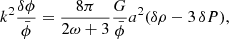
It is common to parameterize the primordial power spectrum (12b) with As. However, as we are interested in predicting the late-time matter power spectrum, it is more natural to ask for “equal power” in BD and GR today than at early times. The normalization of today’s power spectrum is conventionally done in terms of the parameter
 (18)
(18)
where ![Mathematical equation: $ \hat{W}_{\mathrm{R}}(k) = 3 \, [\sin(k R)-kR\cos(k R)] / (k R)^3 $](/articles/aa/full_html/2024/09/aa50050-24/aa50050-24-eq87.gif) is the Fourier transform of the top-hat profile WR(r) = Θ(R − r)/(4πR3/3) with radius R. It is common to define the normalization using the value of σ8, i.e. σR with R = 8 Mpc/h. By pinning
is the Fourier transform of the top-hat profile WR(r) = Θ(R − r)/(4πR3/3) with radius R. It is common to define the normalization using the value of σ8, i.e. σR with R = 8 Mpc/h. By pinning  today6, we get less primordial power
  to compensate for the increased structure growth in BD due to both less Hubble friction EBD < EGR and stronger gravity GBD > GGR (see Fig. 1). Figure 5 shows that using the same As gives a peak in the boost, while using the same σ8 gives a flatter boost.
This shows that the parameterization in Fig. 5a with σ8 and  gives the simplest and most predictable nonlinear boost. As an added bonus, it also deviates the least from its linear counterpart, and we show below that this holds through parameter space.
5. Resulting matter power spectrum boost
We now focus on the boost with the particular parameterization developed in Sect. 4, defaulting to the fiducial parameters in Table 2 (equivalent to the transformation in Fig. 5a). In particular, due to the cosmological constraints ω ≳ 1000 summarized in Table 1, we restricted ourselves to ω ≥ 100 and used the minimum ω = 100 in the fiducial cosmology.
5.1. Understanding the linear boost growth
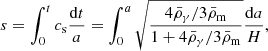
The simplest way to understand the evolution of the linear scale-dependent boost is in terms of the scale-independent growth factor D+(a) from equation (10). During matter domination, the power spectrum scales like 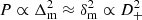 at sub-horizon scales, so
 (19)
(19)
Fig. 6 compares this to the evolution of the full linear boost from early matter domination till today. As seen in Fig. 1, the scalar field in BD begins to move during matter domination, resulting in both less Hubble friction  and stronger gravity GBD > GGR. This gives faster growth in BD!
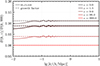 |
Fig. 6. Evolution of the linear matter power spectrum boost from HI_CLASS compared to the scale-independent growth (19) in Fig. 1, starting from a = 10−3 during early matter domination. The boosts are calculated in the fiducial cosmology in Table 2 (equivalent to the transformation in Fig. 5a). Notice that the curves for z = 0 and z = 9 overlap, and that the boost turns around at the peak z = 1.5 in Fig. 1. |
When dark energy takes over, Fig. 1 shows that the expansion accelerates more in BD than in GR with  , while the gravitational strengths GBD → GGR also become equal. This causes the boost to peak around z = 1.5 and then fall off.
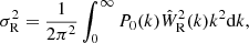
5.2. Cosmological dependence of the nonlinear boost
We now study how the nonlinear boost changes with the cosmological parameters in Table 2. In Fig. 7, we vary one by one parameter away from its fiducial value while keeping the others fixed. Not only is the boost (divided by 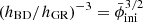 ) very resistant toward parameter changes, but so is its resemblance
 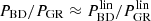 of the linear boost within 1% up to k ≤ 1 h/Mpc, and 2% up to k ≤ 5 h/Mpc.
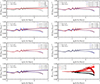 |
Fig. 7. Variation of the matter power spectrum boost (15) at z = 0 as each cosmological parameter is varied away from its fiducial value in Table 2 (equivalent to the transformation in Fig. 5a). The bottom right plot is special; showing the ratio of the nonlinear boost from FML/COLA to the linear boost from HI_CLASS for all boosts in the 7 other plots at more redshifts z = 0.0, 1.5, 3.0. It shows that B ≈ Blin to 1% for k ≤ 1 h/Mpc, and 2% for k ≤ 5 h/Mpc. |
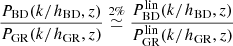
5.3. Linear prediction of the nonlinear boost
Conveniently, this lets us get away with predicting the nonlinear boost 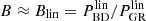 using linear theory and codes, like HI_CLASS. In turn, we can predict the nonlinear power spectrum PBD = Blin ⋅ PGR from an existing nonlinear prediction of PGR. In fact, existing PGR emulators like EUCLIDEMULATOR2 only output the nonlinear correction factor
  and defer multiplication with
  , so it even looks like we can cancel
  and simply calculate
  . However, we still need to calculate
  in order to calculate the σ8 integral (18) from the perturbations to make the parameter transformation θGR(θBD).
We provide the program BD.PY7 that handles these subtleties and predicts the nonlinear BD spectrum from 2 runs of HI_CLASS for the linear spectra BD and GR spectra and 1 run of EUCLIDEMULATOR2 for the nonlinear GR spectrum. This is our main product, and can be used in future fitting to large-scale structure survey data.
5.4. Comparison with existing nonlinear prediction
To demonstrate our program BD.PY, we compared it to the prediction of Joudaki et al. (2022) that we mentioned in Sect. 1. They incorporated BD into HMCODE by tuning the expression for the virial overdensity to match a set of N-body simulations. For their purpose of using KiDS data to constrain the model, the accuracy aim was only a few percent up to k ≲ 1 h/Mpc and 5 − 10% up to k ≲ 10 h/Mpc. Fig. 8 shows that their prediction was (almost) within their tolerance, but produces too little power in BD when trialed with a tighter 1% tolerance.
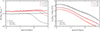 |
Fig. 8. A nonlinear BD-ΛCDM power spectrum (boost) with ω = 100 obtained with our script BD.PY compared to that from an older fitting-formula modification to HMCODE in HI_CLASS from Joudaki et al. (2022), and COLA N-body results from FML. |
6. Conclusion
Despite increasingly tight constraints from small-scale experiments, BD gravity remains interesting at cosmological scales, where constraints are weaker and it approximates more general theories of gravity with screening that falls back to GR at small scales. More precise data from upcoming stage-IV large-scale structure surveys, like Euclid, can increase the competitiveness of cosmological constraints, and shed new light on this situation to illuminate the path forward for constraints on gravity.
In fact, this work began as an effort to train a traditional machine learning emulator for the nonlinear BD matter power spectrum from a set of COLA N-body simulations. Instead, we found that it is possible to predict the nonlinear boost B = PBD/PGR using linear theory and codes if one transforms the cosmological parameters θBD → θGR in a particular way. In detail, by comparing the linear boost with the nonlinear boosts from both COLA and standard N-body simulations, we verified that
This “trick” exploits the boost’s dependence on cosmological parameters to map the nonlinear boost to the linear boost.
This has the advantage that the boost can be computed with cheap linear codes like HI_CLASS, instead of expensive nonlinear N-body methods. When paired with an existing nonlinear PGR predictor, such as EUCLIDEMULATOR2, this paves a simple and efficient path for predicting PBD and constraining BD theory with the precision of upcoming stage-IV large-scale structure surveys. We provide the program BD.PY for this.
A drawback of our approach is that the parameter transformation θBD → θGR requires the emulator PGR(θGR) to cover a broader range of cosmological parameters than that motivated by GR alone. For example, for reasonable input parameters hBD and  , our transformation can request values of hGR and
  that are outside the parameter ranges covered by a GR emulator. To facilitate MG studies, we therefore encourage developers of base GR emulators to “think big” when setting parameter bounds. It would also be valuable to develop a traditional matter power spectrum emulator dedicated to BD, or improve the precision of previous halo modeling approaches.
We also encourage others to investigate whether such simplifying parameter mappings θMG → θGR exist for other MG theories. Our findings could be specific to BD gravity or apply to more theories, perhaps with a similar scale-independent nature. Even if one does not find  “exactly,” investing thought in a clever parameter transformation may still pay off by simplifying the shape of PMG/PGR so that one can obtain it from
  through a fitting formula or ease the training of emulators. This reduces the effort needed to explore alternatives to ΛCDM with MG, so one does not have to duplicate the effort gone into GR for every such alternative.
Including massive neutrinos is straightforward, but previous studies (such as Mauland et al. 2024) have shown that they have little effect on the matter power spectrum boost.
Some authors instead define  in terms of the effective
  . This is natural in BD because their sum is ∑sΩs = 1 at all times, if one defines an effective Ωϕ. However, we opted for the GR definition Ωs = ρs/(3H2/8πG) to minimize confusion and maintain consistency with the HI_CLASS input parameter
  .
.
The FML library is available at https://github.com/HAWinther/FML/, and the COLA N-body code in the subdirectory https://github.com/HAWinther/FML/tree/master/FML/COLASolver.
This RAMSES patch is available at https://github.com/HAWinther/JordanBransDicke.
Strictly speaking, we cannot have  for all species s because
  is constrained by the Friedmann equation, but we have
  at early times, when
  .
.


The BD.PY code is available at https://github.com/hersle/jbd.
Acknowledgments
We thank the Research Council of Norway for their support under grant no. 287772.
References
- Abazajian, K. N., Adshead, P., Ahmed, Z., et al. 2016, ArXiv e-prints [arXiv:1610.02743] [Google Scholar]
- Acquaviva, V., Baccigalupi, C., Leach, S. M., Liddle, A. R., & Perrotta, F. 2005, Phys. Rev. D, 71, 104025 [NASA ADS] [CrossRef] [Google Scholar]
- Alonso, D., Bellini, E., Ferreira, P. G., & Zumalacárregui, M. 2017, Phys. Rev. D, 95, 063502 [NASA ADS] [CrossRef] [Google Scholar]
- Amirhashchi, H., & Yadav, A. K. 2020, Physics of the Dark Universe, 30, 100711 [NASA ADS] [CrossRef] [Google Scholar]
- Angulo, R. E., & Pontzen, A. 2016, MNRAS, 462, L1 [NASA ADS] [CrossRef] [Google Scholar]
- Angulo, R. E., & White, S. D. M. 2010, MNRAS, 405, 143 [NASA ADS] [Google Scholar]
- Angulo, R. E., Zennaro, M., Contreras, S., et al. 2021, MNRAS, 507, 5869 [NASA ADS] [CrossRef] [Google Scholar]
- Archibald, A. M., Gusinskaia, N. V., Hessels, J. W. T., et al. 2018, Nature, 559, 73 [Google Scholar]
- Aricò, G., Angulo, R. E., Contreras, S., et al. 2021, MNRAS, 506, 4070 [CrossRef] [Google Scholar]
- Aricò, G., Angulo, R. E., & Zennaro, M. 2022, Open Res Europe, 2022, 152 [CrossRef] [Google Scholar]
- Avilez, A., & Skordis, C. 2014, Phys. Rev. L, 113, 011101 [NASA ADS] [CrossRef] [Google Scholar]
- Ballardini, M., Finelli, F., Umiltà, C., & Paoletti, D. 2016, JCAP, 2016, 067 [CrossRef] [Google Scholar]
- Ballardini, M., Sapone, D., Umiltà, C., Finelli, F., & Paoletti, D. 2019, JCAP, 2019, 049 [CrossRef] [Google Scholar]
- Ballardini, M., Braglia, M., Finelli, F., et al. 2020, JCAP, 2020, 044 [Google Scholar]
- Ballardini, M., Finelli, F., & Sapone, D. 2022, JCAP, 2022, 004 [CrossRef] [Google Scholar]
- Bellini, E., Barreira, A., Frusciante, N., et al. 2018, Phys. Rev. D, 97, 023520 [NASA ADS] [CrossRef] [Google Scholar]
- Bellini, E., Sawicki, I., & Zumalacárregui, M. 2020, JCAP, 2020, 008 [Google Scholar]
- Bertotti, B., Iess, L., & Tortora, P. 2003, Nature, 425, 374 [Google Scholar]
- Blas, D., Lesgourgues, J., & Tram, T. 2011, JCAP, 2011, 034 [Google Scholar]
- Bose, B., Cataneo, M., Tröster, T., et al. 2020, MNRAS, 498, 4650 [Google Scholar]
- Brando, G., Fiorini, B., Koyama, K., & Winther, H. A. 2022, JCAP, 2022, 051 [CrossRef] [Google Scholar]
- Brans, C., & Dicke, R. H. 1961, Phys. Rev., 124, 925 [NASA ADS] [CrossRef] [Google Scholar]
- Casas, S., Kunz, M., Martinelli, M., & Pettorino, V. 2017, Physics of the Dark Universe, 18, 73 [NASA ADS] [CrossRef] [Google Scholar]
- Cataneo, M., Lombriser, L., Heymans, C., et al. 2019, MNRAS, 488, 2121 [Google Scholar]
- Clifton, T., Ferreira, P. G., Padilla, A., & Skordis, C. 2012, Phys. Rep., 513, 1 [NASA ADS] [CrossRef] [Google Scholar]
- DESI Collaboration 2016, ArXiv e-prints [arXiv:1611.00036] [Google Scholar]
- Dicke, R. H. 1962, Phys. Rev., 125, 2163 [NASA ADS] [CrossRef] [Google Scholar]
- Euclid Collaboration (Knabenhans, M., et al.) 2021, MNRAS, 505, 2840 [NASA ADS] [CrossRef] [Google Scholar]
- Ezquiaga, J. M., & Zumalacárregui, M. 2017, Phys. Rev. L, 119, 251304 [CrossRef] [Google Scholar]
- Fidler, C., Tram, T., Rampf, C., et al. 2017, JCAP, 2017, 043 [CrossRef] [Google Scholar]
- Fiorini, B., Koyama, K., & Baker, T. 2023, JCAP, 2023, 045 [CrossRef] [Google Scholar]
- Freire, P. C. C., Wex, N., Esposito-Farèse, G., et al. 2012, MNRAS, 423, 3328 [NASA ADS] [CrossRef] [Google Scholar]
- Frusciante, N., Pace, F., Cardone, V. F., et al. 2024, A&A, in press, https://doi.org/10.1051/0004-6361/202347526 [NASA ADS] [CrossRef] [EDP Sciences] [Google Scholar]
- Giblin, B., Cataneo, M., Moews, B., & Heymans, C. 2019, MNRAS, 490, 4826 [Google Scholar]
- Heitmann, K., Bingham, D., Lawrence, E., et al. 2016, ApJ, 820, 108 [Google Scholar]
- Horndeski, G. W. 1974, Int. J. Theoret. Phys., 10, 363 [NASA ADS] [CrossRef] [Google Scholar]
- Howlett, C., Manera, M., & Percival, W. J. 2015, Astron. Comput., 12, 109 [NASA ADS] [CrossRef] [Google Scholar]
- Joudaki, S., Ferreira, P. G., Lima, N. A., & Winther, H. A. 2022, Phys. Rev. D, 105, 043522 [NASA ADS] [CrossRef] [Google Scholar]
- Laureijs, R., Amiaux, J., Arduini, S., et al. 2011, ArXiv e-prints [arXiv:1110.3193] [Google Scholar]
- Lawrence, E., Heitmann, K., Kwan, J., et al. 2017, ApJ, 847, 50 [Google Scholar]
- Li, Y.-C., Wu, F.-Q., & Chen, X. 2013, Phys. Rev. D, 88, 084053 [NASA ADS] [CrossRef] [Google Scholar]
- LSST Science Collaboration 2009, ArXiv e-prints [arXiv:0912.0201] [Google Scholar]
- Mauland, R., Winther, H. A., & Ruan, C.-Z. 2024, A&A, 685, A156 [NASA ADS] [CrossRef] [EDP Sciences] [Google Scholar]
- Mead, A. J., Peacock, J. A., Heymans, C., Joudaki, S., & Heavens, A. F. 2015, MNRAS, 454, 1958 [NASA ADS] [CrossRef] [Google Scholar]
- Mead, A. J., Heymans, C., Lombriser, L., et al. 2016, MNRAS, 459, 1468 [Google Scholar]
- Mead, A. J., Brieden, S., Tröster, T., & Heymans, C. 2021, MNRAS, 502, 1401 [Google Scholar]
- Moran, K. R., Heitmann, K., Lawrence, E., et al. 2023, MNRAS, 520, 3443 [NASA ADS] [CrossRef] [Google Scholar]
- Nagata, R., Chiba, T., & Sugiyama, N. 2004, Phys. Rev. D, 69, 083512 [NASA ADS] [CrossRef] [Google Scholar]
- Ooba, J., Ichiki, K., Chiba, T., & Sugiyama, N. 2016, Phys. Rev. D, 93, 122002 [NASA ADS] [CrossRef] [Google Scholar]
- Ooba, J., Ichiki, K., Chiba, T., & Sugiyama, N. 2017, Progr. Theoret. Exp. Phys., 2017, 043E03 [CrossRef] [Google Scholar]
- Orjuela-Quintana, J. B., & Nesseris, S. 2023, JCAP, 2023, 019 [CrossRef] [Google Scholar]
- Perivolaropoulos, L., & Skara, F. 2022, Nat. Astron., 95, 101659 [NASA ADS] [Google Scholar]
- Ruan, C.-Z., Cuesta-Lazaro, C., Eggemeier, A., et al. 2024, MNRAS, 527, 2490 [Google Scholar]
- Sáez-Casares, I., Rasera, Y., & Li, B. 2024, MNRAS, 527, 7242 [Google Scholar]
- Smith, R. E., Peacock, J. A., Jenkins, A., et al. 2003, MNRAS, 341, 1311 [Google Scholar]
- Solà Peracaula, J., Gómez-Valent, A., de Cruz Pérez, J., & Moreno-Pulido, C. 2019, ApJ, 886, L6 [CrossRef] [Google Scholar]
- Solà Peracaula, J., Gómez-Valent, A., de Cruz Pérez, J., & Moreno-Pulido, C. 2020, Class. Quant. Grav., 37, 245003 [CrossRef] [Google Scholar]
- Takahashi, R., Sato, M., Nishimichi, T., Taruya, A., & Oguri, M. 2012, ApJ, 761, 152 [Google Scholar]
- Tassev, S., Zaldarriaga, M., & Eisenstein, D. J. 2013, JCAP, 2013, 036 [Google Scholar]
- Teyssier, R. 2002, A&A, 385, 337 [CrossRef] [EDP Sciences] [Google Scholar]
- Umiltà, C., Ballardini, M., Finelli, F., & Paoletti, D. 2015, JCAP, 2015, 017 [Google Scholar]
- Villaescusa-Navarro, F., Naess, S., Genel, S., et al. 2018, ApJ, 867, 137 [NASA ADS] [CrossRef] [Google Scholar]
- Voisin, G., Cognard, I., Freire, P. C. C., et al. 2020, A&A, 638, A24 [NASA ADS] [CrossRef] [EDP Sciences] [Google Scholar]
- Will, C. M. 2014, Liv. Rev. Relat., 17, 4 [Google Scholar]
- Winther, H. A., Koyama, K., Manera, M., Wright, B. S., & Zhao, G.-B. 2017, JCAP, 2017, 006 [CrossRef] [Google Scholar]
- Winther, H. A., Casas, S., Baldi, M., et al. 2019, Phys. Rev. D, 100, 123540 [CrossRef] [Google Scholar]
- Wu, F.-Q., & Chen, X. 2010, Phys. Rev. D, 82, 083003 [NASA ADS] [CrossRef] [Google Scholar]
- Wu, F.-Q., Qiang, L.-E., Wang, X., & Chen, X. 2010, Phys. Rev. D, 82, 083002 [NASA ADS] [CrossRef] [Google Scholar]
- Yahya, S., Bull, P., Santos, M. G., et al. 2015, MNRAS, 450, 2251 [NASA ADS] [CrossRef] [Google Scholar]
- Zahn, O., & Zaldarriaga, M. 2003, Phys. Rev. D, 67, 063002 [NASA ADS] [CrossRef] [Google Scholar]
- Zumalacárregui, M., Bellini, E., Sawicki, I., Lesgourgues, J., & Ferreira, P. G. 2017, JCAP, 2017, 019 [CrossRef] [Google Scholar]
All Tables
Constraints on the BD parameter ω from various tests, beginning with the Cassini bound from 2003.
Independent cosmological parameters θ for BD-ΛCDM and GR-ΛCDM and, their fiducial values.
All Figures
|
Fig. 1. Evolution of the effective gravitational parameter G, Hubble function E(a) = H(a)/H0, growth factor D(a), and growth rate f(a) = d lnD(a)/d lna from equations (5) and (10) with the scale factor a in the fiducial BD-ΛCDM and GR-ΛCDM cosmologies in Table 2 (equivalent to the transformation in Fig. 5a). The common time of matter-radiation equality is marked by |
| In the text | |
|
Fig. 2. Our BD- or GR-specific simulation pipeline begins from a set of input parameters θBD or θGR. First, they are passed to the Einstein-Boltzmann solver HI_CLASS, which solves the background and perturbations and outputs the linear power spectrum. Next, FML back-scales PHI_CLASS(k,z) from z = 0 to z = zinit, realizes initial conditions for an N-body simulation with the random seed s and evolves it forward with the COLA method on a uniform grid, outputting the nonlinear power spectrum. Finally, FML’s first snapshot can be passed on to RAMSES, which evolves the same initial conditions with the standard N-body method on an adaptive mesh and yields an independent nonlinear power spectrum. |
| In the text | |
|
Fig. 3. Convergence of FML’s boost (15) at z = 0 in the fiducial cosmology in Table 2 (equivalent to the transformation in Fig. 5a), as computational parameters are varied from the fiducial Npart = 5123, Ncell = 5123, Nstep = 30, zinit = 10, and L = 384 Mpc/h. |
| In the text | |
|
Fig. 4. Comparison of the matter power spectrum (boost) obtained from FML using the COLA method on a uniform grid and RAMSES using the standard N-body method on an adaptive grid, in the fiducial cosmology in Table 2 (equivalent to the transformation in Fig. 5a). To compensate for small code differences, we have rescaled all spectra to match the linear HI_CLASS spectrum at their smallest common k. We cut RAMSES’ spectra at increasingly higher k ≤ {1/2, 1, 2}⋅kNyquist as the mesh refinement increases for z = {3, 1.5, 0}. Although P from FML and RAMSES disagree, that error largely cancels in their boosts B = PBD/PGR, which agree to 1% up to k ≲ 5 h/Mpc. |
| In the text | |
|
Fig. 5. Matter power spectrum boost (15) with different parameter transformations θGR = θGR(θBD), where ( |
| In the text | |
|
Fig. 6. Evolution of the linear matter power spectrum boost from HI_CLASS compared to the scale-independent growth (19) in Fig. 1, starting from a = 10−3 during early matter domination. The boosts are calculated in the fiducial cosmology in Table 2 (equivalent to the transformation in Fig. 5a). Notice that the curves for z = 0 and z = 9 overlap, and that the boost turns around at the peak z = 1.5 in Fig. 1. |
| In the text | |
|
Fig. 7. Variation of the matter power spectrum boost (15) at z = 0 as each cosmological parameter is varied away from its fiducial value in Table 2 (equivalent to the transformation in Fig. 5a). The bottom right plot is special; showing the ratio of the nonlinear boost from FML/COLA to the linear boost from HI_CLASS for all boosts in the 7 other plots at more redshifts z = 0.0, 1.5, 3.0. It shows that B ≈ Blin to 1% for k ≤ 1 h/Mpc, and 2% for k ≤ 5 h/Mpc. |
| In the text | |
|
Fig. 8. A nonlinear BD-ΛCDM power spectrum (boost) with ω = 100 obtained with our script BD.PY compared to that from an older fitting-formula modification to HMCODE in HI_CLASS from Joudaki et al. (2022), and COLA N-body results from FML. |
| In the text | |
Current usage metrics show cumulative count of Article Views (full-text article views including HTML views, PDF and ePub downloads, according to the available data) and Abstracts Views on Vision4Press platform.
Data correspond to usage on the plateform after 2015. The current usage metrics is available 48-96 hours after online publication and is updated daily on week days.
Initial download of the metrics may take a while.