| Issue |
A&A
Volume 686, June 2024
|
|
|---|---|---|
| Article Number | A193 | |
| Number of page(s) | 11 | |
| Section | Cosmology (including clusters of galaxies) | |
| DOI | https://doi.org/10.1051/0004-6361/202348639 | |
| Published online | 12 June 2024 | |
Constraining f(R) gravity with cross-correlation of galaxies and cosmic microwave background lensing
Université Paris Cité, CNRS, Astroparticule et Cosmologie, 75013 Paris, France
e-mail: This email address is being protected from spambots. You need JavaScript enabled to view it.
Received:
16
November
2023
Accepted:
6
March
2024
Abstract
We look for signatures of the Hu-Sawicki f(R) modified gravity theory proposed to explain the observed accelerated expansion of the Universe in observations of the galaxy distribution, the cosmic microwave background (CMB), and gravitational lensing of the CMB. We study constraints obtained using observations of only the CMB primary anisotropies before adding the galaxy power spectrum and its cross-correlation with CMB lensing. We show that cross-correlation of the galaxy distribution with lensing measurements is crucial in order to break parameter degeneracies, placing tighter constraints on the model. In particular, we set a strong upper limit on log|fR0|< − 4.61 at 95% confidence level. This means that while the model may explain the accelerated expansion, its impact on large-scale structure closely resembles general relativity (GR). This analysis is the first to make use of the galaxy clustering, CMB lensing, and their cross-correlation power spectra to constrain Hu-Sawicki f(R) gravity. Restricting the analysis to the linear regime, we place a robust constraint that is competitive with other cosmological studies whilst using fewer probes. This study can be seen as a precursor to cross-correlation analyses of f(R) gravity and can be repeated with next-stage surveys, which will benefit from lower noise and hence probe smaller potential deviations from GR.
Key words: gravitational lensing: weak / cosmic background radiation / dark energy / large-scale structure of Universe
© The Authors 2024
 Open Access article, published by EDP Sciences, under the terms of the Creative Commons Attribution License (https://creativecommons.org/licenses/by/4.0), which permits unrestricted use, distribution, and reproduction in any medium, provided the original work is properly cited.
This article is published in open access under the Subscribe to Open model. This email address is being protected from spambots. You need JavaScript enabled to view it. to support open access publication.
1. Introduction
The cause of the late-time accelerated expansion of the Universe is one of the most profound problems facing modern cosmology (Riess et al. 1998; Perlmutter et al. 1999). Many theories have been proposed to explain this phenomenon. The most popular – due to its apparent simplicity – is Λ, the cosmological constant. However, interpretation of the cosmological constant as the energy of the vacuum results in theoretical predictions that are at least 55 orders of magnitude too large (e.g., Carroll et al. 2004; Solà 2013), motivating searches for alternative explanations. One possibility is new gravitational physics (Carroll et al. 2004). In addition to causing the accelerated expansion, modifications to gravity may alter structure formation in the Universe. We constrain a particular model of f(R) gravity (Buchdahl 1970; Starobinsky 1980), which can explain the accelerated expansion of the Universe. To this end, we use observations of galaxy clustering, weak gravitational lensing of the cosmic microwave background (CMB), and temperature and polarization information from the CMB.
Deviations from general relativity (GR) are tightly constrained on the scales of our Solar System (Everitt et al. 2011; Will 2014). Therefore, models of modified gravity must satisfy these constraints on small scales whilst simultaneously modifying gravity on large scales to explain the cosmic acceleration. Carroll et al. (2004) presented a general class of models that can drive cosmic acceleration by replacing the linear dependence of the Einstein-Hilbert action on the Ricci scalar R with a nonlinear function of R (R → R + f(R)). Hu & Sawicki (2007, hereafter HS) presented a class of f(R) models capable of explaining the cosmic acceleration, while evading the strong Solar System constraints through a chameleon mechanism (Khoury & Weltman 2004; Navarro & Van Acoleyen 2007; Faulkner et al. 2007).
Constraints have been placed on HS f(R) gravity using many different complementary observations. Such observations constrain fR0, the value of the cosmological field today; we introduce this parameter in more detail in Sect. 2. In particular, on cosmological scales, HS f(R) was constrained by Cataneo et al. (2015), who obtained the constraint log|fR0|< − 4.79 at the 95% confidence level using cluster number counts in addition to CMB, supernovae, and baryon acoustic oscillation (BAO) data. Hu et al. (2016) also found log|fR0|< − 4.5 using the CMB (temperature, polarization, and lensing), supernovae, BAO, and galaxy weak lensing measurements. Hojjati et al. (2016) obtained the upper bound log|fR0|< − 4.15 at the 95% confidence level using similar observations.
The strongest constraints come from galactic scales. Naik et al. (2019) were able to exclude log|fR0|> − 6.1 using galaxy rotation curves, and Desmond & Ferreira (2020) excluded log|fR0|> − 7.85 based on the analysis of galaxy morphology. Astrophysical and cosmological constraints on HS f(R) gravity can also be found in the review by Lombriser (2014). Finally, Casas et al. (2023) forecast the constraints that will be achievable using observations from Euclid. Despite the strong constraints on HS f(R) gravity from galactic studies, it is still useful to explore deviations from GR on cosmological scales.
Many different tools have been developed to predict the matter power spectrum in HS f(R) gravity. Boltzmann codes that calculate the linear matter power spectrum are mgcamb (Zhao et al. 2009; Hojjati et al. 2011; Zucca et al. 2019; Wang et al. 2023), EFTCAMB (Hu et al. 2014; Raveri et al. 2014), and MGCLASS (Sakr & Martinelli 2022). There are several simulation-based emulators of the matter power spectrum into the mildly nonlinear regime (Winther et al. 2019; Ramachandra et al. 2021; Arnold et al. 2022; Sáez-Casares et al. 2024), and ReACT (Bose et al. 2020, 2023), which uses a halo model reaction framework validated on N-body simulations.
Throughout the present article, we use a model of the Universe that at large scales is homogeneous, isotropic, and flat, as described by the Friedmann-Lemaître-Robertson-Walker metric. Further, we assume three massive degenerate neutrinos with fixed minimal mass ∑mν = 0.06 eV.
In the following section, we review HS f(R) gravity. In Sect. 3, we introduce the observations used in our analysis, and then in Sect. 4 we overview our methodology, including our estimation of the angular power spectrum, our covariance matrix estimation, and how we calculate our likelihood. Our results are presented in Sect. 5, and we outline our conclusions in Sect. 6.
2. Hu-Sawicki f(R) gravity
In f(R) theories of gravity, the Einstein-Hilbert action is modified such that R → R + f(R); therefore in the Jordan frame, the action becomes,
![Mathematical equation: $$ \begin{aligned} S = \int d^4x\sqrt{-g}\left[\frac{R+f(R)}{2\kappa ^2}+\mathcal{L} _{\rm m}\right], \end{aligned} $$](/articles/aa/full_html/2024/06/aa48639-23/aa48639-23-eq1.gif) (1)
(1)
where R is the Ricci scalar; κ = 8πG, with G being the gravitational constant (and the speed of light set to 1); g is the determinant of the spacetime metric; ℒm is the matter Lagrangian; and f is a function of the Ricci scalar. In HS (Hu & Sawicki 2007), f(R) follows a broken power law,
 (2)
(2)
where m is a mass scale given by  with
with  the mean matter density of the Universe, and c1, c2, and n are three dimensionless constants. The derivative of f with respect to the Ricci scalar R is denoted
 (3)
(3)
and can be interpreted as a new scalar field. Hu & Sawicki (2007) showed that a background close to ΛCDM can be recovered by imposing
 (4)
(4)
where ΩΛ and Ωm are the present-day dark energy and matter densities (divided by the critical density) in the ΛCDM cosmology. Imposing this relation, there remain only two free parameters in Eq. (2): n and either c1 or c2. In the high-curvature regime (R ≫ m2), which was shown by Hu & Sawicki (2007) and Oyaizu (2008) to be the relevant regime to describe the background evolution of our Universe given the observed values of ΩΛ and Ωm, Eq. (3) can be written as
 (5)
(5)
which, evaluated at the present-day background, leads to
 (6)
(6)
The fR0 parameter denotes the background value of fR at the present time, which we choose as our free parameter to constrain the model of HS f(R). Additionally, we fix n = 1 as is often assumed in the literature and because ReACT does not allow us to vary this parameter.
For the small values of fR0 probed in this work, the background expansion of the Universe in f(R) is indistinguishable from that in ΛCDM. Instead, we constrain f(R) through its impact on the growth of structure. This can be seen by looking at the modified Poisson equation in f(R):
 (7)
(7)
where a is the cosmological scale factor and  for a metric of the form ds2 = −(1 + 2Φ)dt2 + a2(t)(1 + 2Ψ)dx2 (see e.g., Oyaizu 2008). We see directly that fR/2 can be seen as the potential of the modified gravity force. As mentioned in Sect. 1, this modified Poisson equation approaches the GR expression within the Solar System through the chameleon mechanism (Khoury & Weltman 2004; Hu & Sawicki 2007).
It is worth noting that, unlike other theories of modified gravity, HS f(R), has little effect on the propagation of light in the weak-field limit (e.g., Hojjati et al. 2016).
3. Data
3.1. BOSS galaxies
We used the DR12 data release of the BOSS survey from the SDSS Collaboration (Alam et al. 2015). This large-scale spectroscopic survey was divided into two subsamples, LOWZ and CMASS. LOWZ contains galaxies at low redshift, up to approximately z ≃ 0.45, while CMASS contains higher redshift galaxies (roughly up to z ≃ 0.8) and was constructed to create a sample of galaxies with approximately constant stellar mass. As in Loureiro et al. (2019), we restrict these samples to 0.15 < z < 0.45 and 0.45 < z < 0.8 for LOWZ and CMASS, respectively, such that the two samples do not overlap in redshift. This choice allows us to neglect the covariance between galaxies of LOWZ and CMASS. Using these redshift ranges, and after masking regions of low completeness, the two samples contain 366 576 and 751 067 galaxies, respectively. The redshift distribution of the two samples is shown in Fig. 1.
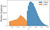 |
Fig. 1. CMASS (blue) and LOWZ (orange) redshift distributions. |
The mask and map making is identical to that used by Kou & Bartlett (2023), who follow Reid et al. (2016) and Loureiro et al. (2019). We transform the MANGLE1 (Swanson et al. 2008) acceptance and veto masks – which are provided with the galaxy catalogs – into high-resolution binary masks in HEALPix2 (Górski et al. 2005; Zonca et al. 2019) format with NSIDE = 8192. The acceptance mask represents the completeness of the observations, while the veto mask excludes regions that could not be observed. A first cut is made to exclude regions with completeness below 0.7, before degrading the resolution of the mask to NSIDE = 4096. A second cut is then applied, such that pixels with completeness below 0.8 are rejected. Finally, the galaxy maps are computed by summing the weighted number of galaxies in each pixel divided by the completeness of the pixel. The weight wtot that is applied to each galaxy takes into account a number of observational effects, including fiber collisions, redshift failures, stellar density, and seeing conditions (more details can be found in Ross et al. 2012). The galaxy overdensity map is
 (8)
(8)
where
 (9)
(9)
where  is the completeness in pixel p.
3.2. Cosmic microwave background temperature and polarization observations
We used observations of the CMB temperature and polarization anisotropies from the Planck satellite, which observed the CMB for about 29 months and covered the full sky. In this work, we made use of the likelihood code as provided by Planck Collaboration V (2020), the cosmological results of which were analyzed in Planck Collaboration VI (2020).
3.3. Cosmic microwave background lensing convergence map
The observed CMB fluctuations are distorted because of gravitational lensing as the CMB photons traverse the Universe. An observational consequence of this is the correlation between different multipoles in both the temperature and polarization anisotropies, which would not be present in the unlensed CMB. The CMB lensing potential can therefore be reconstructed from such correlations (see Lewis & Challinor 2006 for a comprehensive review).
We used the CMB lensing convergence map released by Planck Collaboration VIII (2020). This map was obtained using a minimum variance quadratic estimator based on temperature and polarization maps; it covers about 67% of the sky and led to the detection of lensing at 40σ. The map is provided with a resolution of NSIDE = 4096, together with the associated mask with NSIDE = 2048.
4. Methodology
4.1. Theoretical angular power spectra
We calculated the matter power spectrum in f(R) using two different codes, MGCLASS and ReACT. MGCLASS (Sakr & Martinelli 2022) is a modified version of the Boltzmann code CLASS (Blas et al. 2011) in which the equations of the linear perturbation theory are changed to take into account modifications to gravity. MGCLASS can therefore be used to predict the linear matter power spectrum.
ReACT (Bose et al. 2020, 2023) gives predictions for the nonlinear matter power spectrum in beyond ΛCDM cosmologies, including wCDM, f(R), and DGP gravity. ReACT uses a halo-model-based approach described in Cataneo et al. (2019), such that,
 (10)
(10)
where PNL is the nonlinear matter power spectrum in modified gravity, and  is the so-called nonlinear “pseudo-power spectrum”. This pseudo-power spectrum is defined as a ΛCDM power spectrum with initial conditions chosen such that the ΛCDM linear matter power spectrum matches the modified gravity linear matter power spectrum at a given redshift. This choice was made in order to ensure that the halo mass function in ΛCDM and in the modified gravity theory are similar (which is anticipated given that they have been defined to have exactly the same linear matter power spectrum).
The remaining term in Eq. (10), ℛ, is called the reaction, and describes how the ΛCDM matter power spectrum changes due to the modifications to gravity. The reaction is calculated using the halo model and one-loop perturbation theory. More details can be found in Cataneo et al. (2019) and Bose et al. (2023). When using ReACT to predict the nonlinear modified gravity matter power spectrum, a reliable nonlinear ΛCDM matter power spectrum must be provided. We used the halo-model-based HMCode to obtain such a spectrum (Mead et al. 2015).
For our observations, we computed the galaxy auto power spectrum  , the CMB lensing convergence auto power spectrum
  , and the cross-correlation between the two
  . We also computed the CMB temperature and polarization power spectra, which are sensitive to f(R) gravity through gravitational lensing and the integrated Sachs-Wolfe (ISW) effect. For instance, Zhao et al. (2010) and Kable et al. (2022) indeed showed that the ISW effect is sensitive to gravity, and could be used to probe modified gravity theories, while Cai et al. (2014) specifically studied the impact of f(R) gravity on the ISW effect. The CMB temperature, polarization, and convergence power spectra are predicted by MGCLASS.
As mentioned previously, we assume three massive degenerate neutrinos with fixed minimal mass ∑mν = 0.06 eV to model the CMB and the matter power spectra. Massive neutrinos affect clustering measurements in two different ways. First, they suppress the growth of structure, which results in a decrease in the power spectrum (Eisenstein & Hu 1999). This can be partially compensated by an increase in log|fR0|, so that varying neutrino masses can broaden the constraints we place on log|fR0|. This effect should be small for the present study, as neutrino masses have a greater impact on the nonlinear regime, which we do not use. Second, massive neutrinos are also known to make the galaxy bias scale dependent (e.g., see Saito et al. 2009; Villaescusa-Navarro et al. 2014) but this effect has been shown to be negligible for current data (Vagnozzi et al. 2018; Raccanelli et al. 2019) and is therefore not taken into account in this analysis.
For the galaxy auto- and cross-power spectra, we used the matter power spectrum prediction from either ReACT or MGCLASS. We then modeled the angular power spectra using the Limber approximation (Limber 1953):
 (11)
(11)
 (12)
(12)
where H(z) is the Hubble parameter at redshift z, c is the speed of light, χ is the comoving distance, Pm is the matter power spectrum, and k is the comoving wavenumber. Finally, Wg and Wκ are the galaxy and CMB lensing kernels,
 (13)
(13)
 (14)
(14)
Here, bg is the galaxy bias, (1/ntot)(dn/dz) is the normalized galaxy redshift distribution, H0 is the present value of H, Ωm is the matter density parameter, and z* is the redshift of the surface of last scattering.
Figure 2 shows the effect of changing log|fR0| on the galaxy angular power spectrum using the galaxy redshift distribution of CMASS (see Sect. 3 for more details). It can be seen that HS f(R) gravity increases the formation of structure on small scales, leading to more power in the angular power spectrum at larger multipoles. For a given value of log|fR0|, MGCLASS predicts slightly more power than ReACT, except at the highest multipoles, where power might be missing in the prediction of MGCLASS, as this latter only predicts the linear matter power spectrum. This is also the reason why we do not show the predictions using MGCLASS after the dotted gray line marking the transition into the nonlinear regime (see Sect. 4.4). The nonlinear regime is not used in our analysis as we do not use a theoretical model that can reliably model the galaxy bias in this regime. Although the entire analysis can be performed using MGCLASS alone, we still use ReACT in order to use two independent codes and check the consistency at the level of the cosmological constraints.
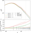 |
Fig. 2. Effect of changing the value of log|fR0| on the auto-power spectrum of CMASS, with all other parameters fixed. The bottom panel shows the difference relative to the nonlinear power spectrum in ΛCDM, together with the 1σ uncertainties of CMASS. Plain lines are obtained using ReACT and the dashed lines with MGCLASS. The gray dotted line shows the limit between the linear and nonlinear regimes. We limit our analysis to the linear regime, but show the theoretical predictions with ReACT. We do not show the predictions with MGCLASS, which fail in this regime. |
4.2. Angular power spectra estimation
The angular cross-correlation power spectrum of two fields A and B is defined as
 (15)
(15)
where aℓm and bℓ′m′ are the spherical harmonic coefficients of fields A and B, respectively, b* denotes the complex conjugate of b, δ is the Kronecker symbol, and ⟨ ⟩ is the ensemble average. Given full sky coverage, this power spectrum can be estimated using
 (16)
(16)
However, in practice, fields A and B are not observed on the full sky, but on a limited sky fraction defined by their masks 𝒲A and 𝒲B, such that what we really observe is  and
and  . It can then be shown (Hivon et al. 2002; Brown et al. 2005) that taking the ensemble average of Eq. (16) with the observed fields
  and
and  gives
gives
 (17)
(17)
where Mℓℓ′ is a coupling matrix that depends on the masks 𝒲A and 𝒲B. It is then possible to recover an unbiased estimate of  by inverting the coupling matrix.
In our analysis, we used the public code NaMaster3 (Alonso et al. 2019) to estimate the power spectra of CMASS and LOWZ, as well as their cross-correlation with the CMB lensing convergence map from Planck. For the CMB lensing auto-correlation, we take the Planck lensing likelihood directly. We also apodized the CMB lensing mask with a scale of 10 arcmin, and we verified that the estimated power spectra do not depend on the apodization scale.
4.3. Noise removal
The measured galaxy angular power spectrum is biased by the shot-noise contribution, and therefore this contribution is subtracted from the estimated power spectrum. The galaxy shot noise is given by
 (18)
(18)
where N is the weighted number of galaxies in each sample.
4.4. Scale cuts
As mentioned in Sect. 4.1, for our cosmological constraints we only use power spectra in the linear regime. This limitation mainly comes from the fact that we use a linear galaxy bias and that this simple modeling is not reliable in the nonlinear regime. To determine the maximum multipole that can be used, we followed the approach of Loureiro et al. (2019). Namely, we used the fiducial cosmology of Planck Collaboration VI (2020) and predicted the theoretical linear and nonlinear power spectra in the ΛCDM model. The nonlinear angular power spectra are obtained using halofit (Smith et al. 2003; Takahashi et al. 2012) to model the nonlinear matter power spectrum and we keep using a linear galaxy bias. We then determined the transition between the linear and nonlinear regimes to correspond to the largest multipole ℓmax such that the relative difference between the linear and nonlinear power spectra is inferior to 5%. The determined scales are presented in Table 1. In practice, we used ℓmax = 200 for CMASS, ℓmax = 100 for LOWZ, and ℓmax = 400 for CMB lensing.
Scale cuts for each power spectrum such that the relative difference between the linear and nonlinear power spectra is inferior to 5%.
Finally, as we used the Limber approximation, which is not valid on large scales, we limited our study to multipoles above ℓmin = 20.
4.5. Covariance matrix
We used a Gaussian covariance matrix following Saraf et al. (2022), allowing us to incorporate nonoverlapping regions of the sky within our cross-correlation analysis:
![Mathematical equation: $$ \begin{aligned} \mathrm{Cov}_{LL^\prime }^{AB,CD} =&\frac{\delta _{LL^\prime }}{(2\ell _L+1)\Delta \ell f_{\rm sky}^{AB}f_{\rm sky}^{CD}}\biggl [f_{\rm sky}^{AC,BD}\left(C_L^{AC}+N_L^{AC}\right)\nonumber \\&\times \left(C_L^{BD}+N_L^{BD}\right) + f_{\rm sky}^{AD,BC} \left(C_L^{AD}+N_L^{AD}\right)\left(C_L^{BC}+N_L^{BC}\right)\biggr ], \end{aligned} $$](/articles/aa/full_html/2024/06/aa48639-23/aa48639-23-eq37.gif) (19)
(19)
where A, B, C, and D label one of the two galaxy density fields g or the CMB lensing convergence field κ, and  is the sky fraction common to fields A and B.
We estimated an initial covariance matrix using Eq. (19) with the observed power spectra. We then used this covariance matrix to fit our theoretical model to the observations, and then determined a second covariance matrix using the best-fit theoretical power spectra from the first analysis. This procedure reduces the sensitivity of the covariance matrix to the noise in the estimated power spectra.
4.6. Likelihood
Our log-likelihood is the sum of the log-likelihood of the galaxy power spectra and the galaxy – CMB lensing cross-correlations, which we denote lnℒ2 × 2 pt here, the Planck log-likelihood for temperature and polarization (Planck Collaboration V 2020), lnℒPlanck, and the Planck CMB lensing (Planck Collaboration VIII 2020) likelihood, lnℒPlanck lensing:
 (20)
(20)
The name 2 × 2 pt comes from the fact that it is the combination of two different types of two-point statistics ( and
and  ). The third two-point statistic is the Planck lensing power spectrum,
  , making our analysis a 3 × 2 pt analysis in combination with the Planck temperature and polarisation likelihood.
We adopt a Gaussian for the 2 × 2 pt likelihood,
![Mathematical equation: $$ \begin{aligned} \ln {\mathcal{L} ^{2\times 2\,\mathrm{pt}}} = -\frac{1}{2}\left[\left(X(\theta )-X^\mathrm{obs}\right)^\mathrm{T}C^{-1}\left(X(\theta )-X^\mathrm{obs}\right)\right], \end{aligned} $$](/articles/aa/full_html/2024/06/aa48639-23/aa48639-23-eq43.gif) (21)
(21)
where XT denotes the transpose of vector X, θ is the parameter vector, C is the covariance matrix, and X is a concatenation of power spectra such that
 (22)
(22)
The likelihood ℒPlanck contains the likelihood for the TT, TE, and EE power spectra. We neglected the covariance between  and
and  (as is done, for instance, in Abbott et al. 2023), which is motivated by the fact that the
  is estimated on a much larger sky fraction than
  , and that CMB lensing power comes mainly from redshifts greater than 0.8, where we do not have any galaxies in either of the two samples.
4.7. Priors
We used flat priors for all of the cosmological parameters, namely ωc, ωb, h, τreio, log1010As, and ns, as well as for the two galaxy bias parameters, for LOWZ and CMASS, and log|fR0|, for which we impose −7 < log|fR0|< 0. We use the recommended priors for the calibration and nuisance parameters required by Planck’s likelihood. In total, we end up with 30 free parameters (the 6 parameters of ΛCDM, log|fR0|, 2 galaxy bias parameters, and 21 calibration and nuisance parameters). We then used the Monte Carlo Markov chain (MCMC) sampler emcee4 (Foreman-Mackey et al. 2013) to sample the resulting posterior distributions.
4.8. Computing prior-independent constraints
As shown in Sect. 5, in many cases we are only able to put upper bounds on log|fR0|. It is therefore nontrivial to estimate the 95% constraint on log|fR0|, because the percentile depends strongly on the lower value of the prior. This arises because the posterior on log|fR0| at low values is nonzero (and almost flat). Therefore, without a lower bound on the prior, very low values of log|fR0| would be explored rather than more interesting regions of the posterior, which would in turn be poorly sampled. This choice of lower limit for log|fR0| changes the estimated 95th percentile.
In order to resolve this issue, we followed the approach of Piga et al. (2023), who rely on Gordon & Trotta (2007). We considered the ratio of the marginalized posterior and our prior,
 (23)
(23)
where x is the parameter we wish to constrain (in our case log|fR0|), d is the data, p the prior, and 𝒫 the posterior. Then, for two different values of x, for example x1 and x2, we applied Bayes theorem to obtain
 (24)
(24)
where B is the Bayes factor and ℒ(d|x) is the marginalized likelihood of the data for x. The Bayes factor, which quantifies the support for the model with x = x1 over the model with x = x2, is therefore prior independent.
Gordon & Trotta (2007) showed that B(x1, x2) = 2.5 means that the model with x = x1 is favored over the model with x = x2 at 95%. We then fixed x1 to its lower bound of log|fR0|= − 7 and searched for the value of x2 such that B(x1, x2) = 2.5. Using this method, we are able to compute 95% confidence intervals that do not depend on the prior. We show that this is indeed the case in Sect. 5.2.4, where we vary the prior used in the analysis.
5. Results
In this section, we present our results for different combinations of observations, with different choices of binnings, theoretical power spectra, and nuisance parameters. The upper limits we place on log|fR0| are shown in Table 2. The corner plot for the fiducial 3 × 2 pt + CMB analysis, obtained thanks to the use of GetDist5 (Lewis 2019), is shown in Fig. 3.
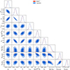 |
Fig. 3. Constraints and degeneracies on all parameters when using observations of the CMB and 3 × 2 pt observables modeled with MGCLASS (blue) or ReACT (red). The contours correspond to the 68th and 95th percentiles of the posterior samples. |
Constraints on log|fR0| obtained in the different cases.
For clarity, we always modeled the CMB temperature, polarization, and lensing using MGCLASS, while we modeled the galaxy power spectra and the galaxy – CMB lensing power spectra using either MGCLASS or ReACT. We did not model the CMB power spectra (including lensing) with ReACT as this code can only make predictions for the matter power spectrum at redshifts z < 2.5.
5.1. Results from CMB only
We first look at the constraints obtained on log|fR0| when using only observations of the CMB. First, we used the CMB temperature and polarization power spectra. These are sensitive to f(R) gravity through the imprint of the ISW effect and gravitational lensing. Lensing is the dominant effect and causes a smoothing of the acoustic peaks (for more detail, see Lewis & Challinor 2006). This is distinct from the CMB lensing convergence reconstruction described in Sect. 3.3. As f(R) increases the power in the lensing potential, f(R) models will have a larger smoothing effect on the CMB.
With just the CMB temperature and polarization observations, we find a strong preference for a nonzero value of fR0 at more than 3σ: we obtain a best-fit value of log|fR0|= − 2.35, with the bounds −3.09 < log|fR0|< − 1.88 at 95% and −5.76 < log|fR0|< − 1.64 at 99.7% confidence levels. The marginalized posterior for log|fR0| is shown in Fig. 4, where we see a clear peak at log|fR0|= − 2.35. This is not a new result and has been shown by other authors; for example Dossett et al. (2014) and Hojjati et al. (2016).
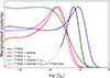 |
Fig. 4. Marginalized posterior of log|fR0| using observations of Planck modeled with MGCLASS. TTTEEE refers to the temperature and polarization power spectra of Planck, “lensing” to the addition of the CMB lensing power spectrum, and Alens to the inclusion of the lensing amplitude. “Alens in TTTEEE only” means that the effect of Alens on the observed CMB lensing convergence power spectrum is not taken into account; only the CMB temperature and polarization power spectra are affected by Alens (see the text for details). |
However, when we add the CMB lensing power spectrum, which is estimated from the mode mixing in the primary CMB (as described in Sect. 3.3), the large values of log|fR0| are excluded, and instead we set an upper limit on log|fR0|: log|fR0|< − 2.31 at 95% confidence (computed following the approach described in Sect. 4.8).
We clearly see that the CMB lensing convergence power spectrum is consistent with GR and low log|fR0| values, while the smoothing of the acoustic peaks in the CMB temperature and polarization anisotropies induces a higher value of log|fR0|. This issue (or tension) is closely related to the Planck Alens tension (Planck Collaboration VI 2020).
The Alens parameter was introduced by Calabrese et al. (2008) as a phenomenological parameter scaling the CMB lensing potential amplitude as
 (25)
(25)
and it therefore changes the amplitude of the CMB lensing convergence power spectrum, and also the smoothing in the temperature and polarization power spectra. As a result, varying Alens has an effect on  but also on
  ,
,  , and
, and  . It was shown in Planck Collaboration VI (2020) that the CMB lensing convergence power spectrum is perfectly compatible with Alens = 1, which is not the case for the temperature and polarization power spectra. For instance, the 1σ constraint that Planck Collaboration VI (2020) find using the TT, TE, EE+low E likelihood is Alens = 1.180 ± 0.065, which is in tension with Alens = 1 at 2.8σ. Interestingly, the log|fR0| tension is larger than the Alens tension. This suggests that the modification of the lensing potential by HS f(R) better describes the smoothing of the CMB than the simple rescaling of the potential with Alens.
We further elucidated the relation between Alens and log|fR0| by running the Planck CMB TTTEEE likelihood with both parameters. Figure 4 shows the result as the blue curve. The constraints on log|fR0| are broadened, with low values of log|fR0| that are compatible with GR. However, the posterior remains consistent with higher values of log|fR0|. Figure 5 illustrates the degeneracy between Alens and log|fR0|.
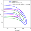 |
Fig. 5. Degeneracy between Alens and log|fR0| for different observation combinations. Those include CMB temperature and polarization only (blue); CMB temperature, polarization, and lensing (green). The case when Alens is considered as a systematic effect and is applied only to the primary CMB anisotropies is also shown in magenta. The contours correspond to the 68th and 95th percentiles of the posterior samples. |
The green and magenta curves in Fig. 4 show the posteriors obtained when adding the CMB lensing convergence power spectrum likelihood. The difference between the two curves is that for the magenta curve, the effect of Alens is only applied to the temperature and polarization power spectra. In this case, we do not take into account the effect of Alens on the amplitude of the observed CMB lensing convergence power spectrum  but only the effects of the excess smoothing observed on the temperature and polarization spectra. Our assumption is that we observe Alens > 1 in TTTEEE, not because of a lensing excess but as the effect of an unknown observational systematic uncertainty. In both cases, the posteriors agree with GR, and we can put an upper limit on the value of log|fR0|.
We show the degeneracy between log|fR0| and Alens in these two cases in Fig. 5. When Alens is treated as a systematic uncertainty (magenta contours), we recover high Alens values because the convergence power spectrum constrains log|fR0| to low values where it cannot reproduce the smoothing observed in the acoustic peaks. These results clearly show that HS f(R) gravity cannot explain the Alens tension, which is in agreement with the findings of Hojjati et al. (2016).
5.2. Results from combined CMB and 3 × 2 pt observations
We now present our fiducial analysis, that is, the combination of the CMB (temperature and polarization power spectra) and the 3 × 2 pt analysis (CMB convergence power spectrum, galaxy power spectrum, and the cross-correlation between the two). In this section, the value of Alens is fixed to 1 unless stating otherwise.
Figure 6 gives the marginalized posterior of log|fR0| obtained when using either MGCLASS (black curve) or ReACT (red curve) when modeling the 2 × 2 pt observables ( and
and  ) and we reiterate that the CMB lensing convergence auto power spectrum is always modeled using MGCLASS. The 95% confidence level constraints are log|fR0|< − 4.12 and log|fR0|< − 4.61 with MGCLASS and ReACT, respectively. These constraints are consistent with GR and are much tighter than when using only the CMB observations. This also excludes HS f(R) as an explanation of the Alens tension as solving the tension would require high values of log|fR0|, which are now excluded.
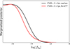 |
Fig. 6. Marginalized posterior of log|fR0| using observations of CMB temperature and polarization, and the 3 × 2 pt observables (CMB lensing, galaxy distribution, and their cross-correlation). The CMB observations including the CMB lensing auto power spectrum are always modeled using MGCLASS, while the galaxy power spectra and the galaxy–CMB lensing cross-correlations are modeled with ReACT (red) or MGCLASS (black). |
The difference between MGCLASS and ReACT is also evident in Fig. 2. MGCLASS only predicts the linear matter power spectrum, whereas ReACT predicts the nonlinear power spectrum. Although our scale cuts were chosen to minimise the effects of nonlinear structure formation, it seems likely that the origin of this difference here arises from the mildly nonlinear regime where the MGCLASS predictions have less power than those of ReACT. Therefore, our MGCLASS constraint is likely too conservative and hence not as strong as it should be.
Figure 3 shows the marginalized two-dimensional posteriors on all parameters when using MGCLASS (blue) or ReACT (red). We see that the posteriors agree well for most parameters. We also see that log|fR0| exhibits a degeneracy with the galaxy bias parameters. This arises because both parameters change the amplitude of the galaxy power spectra. However, the parameters are not completely degenerate, as log|fR0| also changes the shape of the power spectra, and the cross-correlation separates the two effects to a certain extent, as explored in the following subsection.
Figure 7 shows the measured angular power spectra (orange) and the theoretical best fit (blue) using MGCLASS. The model fits the data well, except at the largest scales for the cross-correlation between the CMB lensing of Planck and the galaxies of CMASS, where the amplitude of the theoretical power spectrum is larger than the amplitude of the observation. This result has been observed in previous studies (Pullen et al. 2016; Singh et al. 2017; Kou & Bartlett 2023). We see that HS f(R) is unable to resolve this problem.
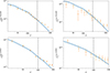 |
Fig. 7. Measured angular power spectra (orange) and best fit (blue) obtained using MGCLASS, as a function of multipole. The gray dashed line represents the limit between the linear and nonlinear regimes. We only used multipoles below this limit in this analysis. We note the different multipole ranges for CMASS and LOWZ. |
The constraints on log|fR0| are consistent and competitive with previous studies using galaxy clustering observations, such as Hu et al. (2016). The tightest constraint obtained by these latter authors is log|fR0|< − 4.5 when combining observations of the CMB (temperature, polarization, lensing), supernovae, BAO measurements (including but not limited to BAO measurements of LOWZ and CMASS), and galaxy weak lensing shear correlation functions estimated from the Canada-France-Hawaii Telescope Lensing Survey (Heymans et al. 2013). The cross-correlation of galaxy–CMB lensing spectra enables us to obtain competitive constraints with a reduced data set.
5.2.1. Benefit of the cross-correlation
In order to isolate the advantage of the cross-correlation, we performed the analysis without the cross-correlation power spectra. The cross-correlation is primarily useful in reducing the degeneracy between log|fR0| and the galaxy bias parameters. The degeneracy is reduced as  is proportional to
  , while
  is proportional to bg (see Eqs. (13) and (14)). This effect is seen in Fig. 8 where the red contours do not contain the cross-correlation and the blue contours do. As a result, the 95% constraint obtained without the cross-correlation is log|fR0|< − 2.95, compared to log|fR0|< − 4.12 with the cross-correlation, which is an improvement of more than an order of magnitude.
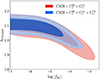 |
Fig. 8. Marginalized constraints on log|fR0| and the galaxy bias of CMASS when using CMB observations and the full 3 × 2 pt observables (blue) or only the galaxy and CMB lensing auto power spectra (red). It can be seen that adding the galaxy–CMB lensing cross-correlation reduces the degeneracy between the two parameters. Those contours correspond to the 68th and 95th percentiles of the posterior samples. |
5.2.2. Result including Alens as a systematic uncertainty
As was shown in Sect. 5.1, HS f(R) cannot explain the Alens tension. When the 2 × 2 pt observations are added, log|fR0| is constrained to even smaller values, which further rules out this kind of modified gravity as a resolution to the Alens tension. As it has been suggested that Alens could be due to a systematic error (Planck Collaboration VI 2020) rather than a physical effect, we also performed our analysis with Alens on the CMB temperature and polarization power spectra only. Our expectation is that this will give tighter constraints, because Alens can explain the excess of smoothing in the CMB temperature and polarization power spectra without the need for a large value of log|fR0|. The resulting marginalized contours on Alens and log|fR0| are shown in Fig. 9. As expected, Alens > 1 is more likely in this configuration. Unsurprisingly, the 95% constraint of log|fR0|< − 4.24 is tighter than the fiducial constraint (log|fR0|< − 4.12).
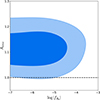 |
Fig. 9. Marginalized constraints on log|fR0| and Alens, where Alens is considered as a systematic effect and is only applied to the CMB temperature and polarization anisotropies. Here, the 3 × 2 pt observables are included, but are not affected by Alens. A value of Alens > 1 is still preferred. The contours correspond to the 68th and 95th percentiles of the posterior samples. |
5.2.3. Effect of the binning scheme
We examined how changing the binning scheme impacts our constraints. In particular, we defined three binning schemes, namely Δℓ = 10, Δℓ = 20 (the fiducial case), and an unequal binning scheme with an average  . The marginalized posteriors on log|fR0| obtained with the three different binning schemes are presented in Fig. 10. We see that the constraints become tighter as Δℓ decreases. The use of narrow multipole bin widths makes it possible to better use the shape of the power spectra to constrain f(R) gravity. The 95% confidence constraints are log|fR0|< − 4.18, log|fR0|< − 4.12, and log|fR0|< − 3.84 for Δℓ = 10, Δℓ = 20, and
  , respectively. All of our constraints are summarized in Table 2.
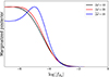 |
Fig. 10. Marginalized posterior of log|fR0| using MGCLASS depending on the binning scheme used. The constraints become tighter as Δℓ decreases. |
5.2.4. Effect of the priors
Our 95% confidence intervals rely on the approach described in Sect. 4.8, the aim of which is to build prior-independent confidence intervals. In order to check that our constraints are indeed prior independent, we ran a second MCMC analysis in the fiducial setup, with a flat prior, −9 < log|fR0|< 0 (instead of the previous −7 < log|fR0|< 0). The posteriors (normalized by the average value of the plateau) are shown in Fig. 11. It can be seen that the 95% constraint is largely insensitive to the lower bound on the prior. More precisely, the constraint using the new prior is log|fR0|< − 4.17, which is close to the limit log|fR0|< − 4.12 that we found with the previous prior.
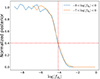 |
Fig. 11. Posteriors of log|fR0| normalized by the average value of the plateau using flat priors between −7 and 0 (orange) or between −9 and 0 (blue). The red dashed lines correspond to the 95% confidence level. |
The approach described in Sect. 4.8 indeed produces constraints independent of the adopted prior. In contrast, if we were to directly use the 95th percentile of the samples, the values associated to each prior (lower bound at −7 or −9) would be −3.93 and −4.27, respectively. This dependence on the choice of prior demonstrates the danger in determining the constraints directly from the sample percentiles; for instance, we extract a tighter constraint when the lower bound of the prior is lower. This finding is intuitive, because by decreasing the lower bound on the prior, we allow the MCMC walkers to explore lower values in parameter space; the posterior distribution therefore shifts towards lower parameter values and consequently the 95th percentile becomes lower as well.
5.2.5. Comparison of other cosmological parameters with ΛCDM
We also look at how the other parameters change when moving from the ΛCDM model to HS f(R) gravity. This can firstly be seen in Fig. 3, which shows the degeneracies between the parameters included in the analysis, as low values of log|fR0| are very close to the ΛCDM model. Apart from the strong degeneracy between log|fR0| and galaxy biases (mentioned previously in Sect. 5.2), there is no important degeneracy between log|fR0| and any of the other cosmological parameters. This is because the majority of the parameters are strongly constrained by the CMB (temperature and polarization) observations, while log|fR0| is constrained by the galaxy power spectra and cross-correlations with CMB lensing.
Table 3 shows the marginalized medians and 68% confidence intervals of each parameter apart from log|fR0| where the results are presented in Table 2. The constraints presented in Table 3 were obtained in the fiducial (CMB + 3 × 2 pt) setup using MGCLASS in the case of HS f(R) gravity as well as in the ΛCDM model. We note that the constraints stated in this table are directly computed from the 68th percentiles of the posteriors without using the approach described in Sect. 4.8. As a result, the constraints stated for the parameters could depend on the prior used for log|fR0| if the parameter is correlated with log|fR0|. This is the case for the galaxy biases, but we observe no significant correlation between log|fR0| and the other parameters, and therefore this should not be an issue. It can be seen that the marginalized medians of each parameter do not change significantly when moving from ΛCDM to f(R) gravity. Table 3 also shows that the constraints are slightly degraded when log|fR0| is added to the analysis compared to the ΛCDM case; however, as already mentioned, this effect is small, as most parameters are constrained by CMB observations, which are not as sensitive to f(R) gravity as galaxy power spectra.
Median and 68% confidence intervals of each parameter in HS f(R) and ΛCDM models.
6. Conclusion
Modified gravity is a possible explanation for the observed accelerated expansion of the Universe (Carroll et al. 2004). Hu-Sawicki (HS) f(R) gravity (Hu & Sawicki 2007) is an attractive example, motivating searches for other possible observational signatures of the model. We looked for such signatures in terms of deviations from the predictions of general relativity in large-scale structure observations in a combined analysis of CMB, galaxy, and CMB lensing measurements.
If the HS f(R) model is to explain the accelerated expansion, the key parameter is log|fR0|. Primary CMB observations alone constrain this parameter through the ISW effect and smoothing of the temperature and polarization anisotropies by gravitational lensing. In agreement with previous analyses, we find that measurements by Planck lead to high values of log|fR0|, which would imply a remarkable deviation from general relativity (see Sect. 5.1). However, this is not the case when the CMB lensing convergence power spectrum is added, reflecting tension between the effects of lensing on the primary anisotropies and the reconstructed lensing power spectrum. This tension is closely related to the problem known as Alens. We illustrate this by exhibiting the degeneracy between log|fR0| and Alens. This analysis also demonstrates that HS f(R) alone cannot resolve this tension.
Setting Alens = 1 and adding galaxy power spectra from BOSS and their cross-correlation with CMB lensing, we then constrain log|fR0|< − 4.61 at 95% confidence (Sect. 5.2). This is our central result. It means that while HS f(R) may still explain the accelerated expansion, there is no signature of the model in current observations of large-scale structure; the model predictions do not substantially deviate from those of general relativity.
We also show that the cross-correlation of galaxy and lensing measurements is essential in breaking the degeneracy between galaxy bias and log|fR0|. Incorporating this cross-correlation improves the constraint on |fR0| by more than an order of magnitude (Sect. 5.2.1).
This study is the first to make use of the cross-correlation between CMB lensing and galaxy measurements to constrain HS f(R) gravity. It paves the way for future large-scale galaxy surveys to place more stringent constraints, as they will benefit from lower noise and use galaxy lensing in addition to CMB lensing.
Acknowledgments
We thank Benjamin Bose for his help in using the ReACT code. We acknowledge the use of the python libraries matplotlib (Hunter 2007), numpy (Harris et al. 2020), and scipy (Virtanen et al. 2020). Some of the results in this paper have been derived using the healpy and HEALPix packages (Górski et al. 2005).
References
- Abbott, T. M. C., Aguena, M., Alarcon, A., et al. 2023, Phys. Rev. D, 107, 023531 [NASA ADS] [CrossRef] [Google Scholar]
- Alam, S., Albareti, F. D., Allende Prieto, C., et al. 2015, ApJS, 219, 12 [Google Scholar]
- Alonso, D., Sanchez, J., Slosar, A., & LSST Dark Energy Science Collaboration 2019, MNRAS, 484, 4127 [NASA ADS] [CrossRef] [Google Scholar]
- Arnold, C., Li, B., Giblin, B., Harnois-Déraps, J., & Cai, Y.-C. 2022, MNRAS, 515, 4161 [CrossRef] [Google Scholar]
- Blas, D., Lesgourgues, J., & Tram, T. 2011, JCAP, 2011, 034 [Google Scholar]
- Bose, B., Cataneo, M., Tröster, T., et al. 2020, MNRAS, 498, 4650 [Google Scholar]
- Bose, B., Tsedrik, M., Kennedy, J., et al. 2023, MNRAS, 519, 4780 [NASA ADS] [CrossRef] [Google Scholar]
- Brown, M. L., Castro, P. G., & Taylor, A. N. 2005, MNRAS, 360, 1262 [NASA ADS] [CrossRef] [Google Scholar]
- Buchdahl, H. A. 1970, MNRAS, 150, 1 [NASA ADS] [Google Scholar]
- Cai, Y.-C., Li, B., Cole, S., Frenk, C. S., & Neyrinck, M. 2014, MNRAS, 439, 2978 [NASA ADS] [CrossRef] [Google Scholar]
- Calabrese, E., Slosar, A., Melchiorri, A., Smoot, G. F., & Zahn, O. 2008, Phys. Rev. D, 77, 123531 [NASA ADS] [CrossRef] [Google Scholar]
- Carroll, S. M., Duvvuri, V., Trodden, M., & Turner, M. S. 2004, Phys. Rev. D, 70, 043528 [NASA ADS] [CrossRef] [Google Scholar]
- Casas, S., Cardone, V. F., Sapone, D., et al. 2023, A&A, submitted [arXiv:2306.11053] [Google Scholar]
- Cataneo, M., Rapetti, D., Schmidt, F., et al. 2015, Phys. Rev. D, 92, 044009 [NASA ADS] [CrossRef] [Google Scholar]
- Cataneo, M., Lombriser, L., Heymans, C., et al. 2019, MNRAS, 488, 2121 [Google Scholar]
- Desmond, H., & Ferreira, P. G. 2020, Phys. Rev. D, 102, 104060 [NASA ADS] [CrossRef] [Google Scholar]
- Dossett, J., Hu, B., & Parkinson, D. 2014, JCAP, 2014, 046 [CrossRef] [Google Scholar]
- Eisenstein, D. J., & Hu, W. 1999, ApJ, 511, 5 [Google Scholar]
- Everitt, C. W. F., Debra, D. B., Parkinson, B. W., et al. 2011, Phys. Rev. Lett., 106, 221101 [NASA ADS] [CrossRef] [Google Scholar]
- Faulkner, T., Tegmark, M., Bunn, E. F., & Mao, Y. 2007, Phys. Rev. D, 76, 063505 [NASA ADS] [CrossRef] [Google Scholar]
- Foreman-Mackey, D., Hogg, D. W., Lang, D., & Goodman, J. 2013, PASP, 125, 306 [Google Scholar]
- Gordon, C., & Trotta, R. 2007, MNRAS, 382, 1859 [CrossRef] [Google Scholar]
- Górski, K. M., Hivon, E., Banday, A. J., et al. 2005, ApJ, 622, 759 [Google Scholar]
- Harris, C. R., Millman, K. J., van der Walt, S. J., et al. 2020, Nature, 585, 357 [NASA ADS] [CrossRef] [Google Scholar]
- Heymans, C., Grocutt, E., Heavens, A., et al. 2013, MNRAS, 432, 2433 [Google Scholar]
- Hivon, E., Górski, K. M., Netterfield, C. B., et al. 2002, ApJ, 567, 2 [NASA ADS] [CrossRef] [Google Scholar]
- Hojjati, A., Pogosian, L., & Zhao, G.-B. 2011, JCAP, 2011, 005 [CrossRef] [Google Scholar]
- Hojjati, A., Plahn, A., Zucca, A., et al. 2016, Phys. Rev. D, 93, 043531 [NASA ADS] [CrossRef] [Google Scholar]
- Hu, W., & Sawicki, I. 2007, Phys. Rev. D, 76, 064004 [CrossRef] [Google Scholar]
- Hu, B., Raveri, M., Frusciante, N., & Silvestri, A. 2014, Phys. Rev. D, 89, 103530 [Google Scholar]
- Hu, B., Raveri, M., Rizzato, M., & Silvestri, A. 2016, MNRAS, 459, 3880 [Google Scholar]
- Hunter, J. D. 2007, Comput. Sci. Eng., 9, 90 [NASA ADS] [CrossRef] [Google Scholar]
- Kable, J. A., Benevento, G., Frusciante, N., De Felice, A., & Tsujikawa, S. 2022, JCAP, 2022, 002 [CrossRef] [Google Scholar]
- Khoury, J., & Weltman, A. 2004, Phys. Rev. D, 69, 044026 [CrossRef] [Google Scholar]
- Kou, R., & Bartlett, J. G. 2023, A&A, 675, A149 [NASA ADS] [CrossRef] [EDP Sciences] [Google Scholar]
- Lewis, A. 2019, arXiv e-prints [arXiv:1910.13970] [Google Scholar]
- Lewis, A., & Challinor, A. 2006, Phys. Rep., 429, 1 [Google Scholar]
- Limber, D. N. 1953, ApJ, 117, 134 [NASA ADS] [CrossRef] [Google Scholar]
- Lombriser, L. 2014, Ann. Phys., 264, 259 [NASA ADS] [CrossRef] [Google Scholar]
- Loureiro, A., Moraes, B., Abdalla, F. B., et al. 2019, MNRAS, 485, 326 [NASA ADS] [CrossRef] [Google Scholar]
- Mead, A. J., Peacock, J. A., Heymans, C., Joudaki, S., & Heavens, A. F. 2015, MNRAS, 454, 1958 [NASA ADS] [CrossRef] [Google Scholar]
- Naik, A. P., Puchwein, E., Davis, A.-C., Sijacki, D., & Desmond, H. 2019, MNRAS, 489, 771 [NASA ADS] [CrossRef] [Google Scholar]
- Navarro, I., & Van Acoleyen, K. 2007, JCAP, 2007, 022 [CrossRef] [Google Scholar]
- Oyaizu, H. 2008, Phys. Rev. D, 78, 123523 [NASA ADS] [CrossRef] [Google Scholar]
- Perlmutter, S., Aldering, G., Goldhaber, G., et al. 1999, ApJ, 517, 565 [Google Scholar]
- Piga, L., Marinucci, M., D’Amico, G., et al. 2023, JCAP, 2023, 038 [CrossRef] [Google Scholar]
- Planck Collaboration V. 2020, A&A, 641, A5 [NASA ADS] [CrossRef] [EDP Sciences] [Google Scholar]
- Planck Collaboration VI. 2020, A&A, 641, A6 [NASA ADS] [CrossRef] [EDP Sciences] [Google Scholar]
- Planck Collaboration VIII. 2020, A&A, 641, A8 [NASA ADS] [CrossRef] [EDP Sciences] [Google Scholar]
- Pullen, A. R., Alam, S., He, S., & Ho, S. 2016, MNRAS, 460, 4098 [CrossRef] [Google Scholar]
- Raccanelli, A., Verde, L., & Villaescusa-Navarro, F. 2019, MNRAS, 483, 734 [NASA ADS] [CrossRef] [Google Scholar]
- Ramachandra, N., Valogiannis, G., Ishak, M., Heitmann, K., & LSST Dark Energy Science Collaboration 2021, Phys. Rev. D, 103, 123525 [CrossRef] [Google Scholar]
- Raveri, M., Hu, B., Frusciante, N., & Silvestri, A. 2014, Phys. Rev. D, 90, 043513 [Google Scholar]
- Reid, B., Ho, S., Padmanabhan, N., et al. 2016, MNRAS, 455, 1553 [NASA ADS] [CrossRef] [Google Scholar]
- Riess, A. G., Filippenko, A. V., Challis, P., et al. 1998, AJ, 116, 1009 [Google Scholar]
- Ross, A. J., Percival, W. J., Sánchez, A. G., et al. 2012, MNRAS, 424, 564 [Google Scholar]
- Sáez-Casares, I., Rasera, Y., & Li, B. 2024, MNRAS, 527, 7242 [Google Scholar]
- Saito, S., Takada, M., & Taruya, A. 2009, Phys. Rev. D, 80, 083528 [NASA ADS] [CrossRef] [Google Scholar]
- Sakr, Z., & Martinelli, M. 2022, JCAP, 2022, 030 [CrossRef] [Google Scholar]
- Saraf, C. S., Bielewicz, P., & Chodorowski, M. 2022, MNRAS, 515, 1993 [NASA ADS] [CrossRef] [Google Scholar]
- Singh, S., Mandelbaum, R., & Brownstein, J. R. 2017, MNRAS, 464, 2120 [Google Scholar]
- Smith, R. E., Peacock, J. A., Jenkins, A., et al. 2003, MNRAS, 341, 1311 [Google Scholar]
- Solà, J. 2013, J. Phys. Conf. Ser., 453, 012015 [CrossRef] [Google Scholar]
- Starobinsky, A. A. 1980, Phys. Lett. B, 91, 99 [Google Scholar]
- Swanson, M. E. C., Tegmark, M., Blanton, M., & Zehavi, I. 2008, MNRAS, 385, 1635 [Google Scholar]
- Takahashi, R., Sato, M., Nishimichi, T., Taruya, A., & Oguri, M. 2012, ApJ, 761, 152 [Google Scholar]
- Vagnozzi, S., Brinckmann, T., Archidiacono, M., et al. 2018, JCAP, 2018, 001 [CrossRef] [Google Scholar]
- Villaescusa-Navarro, F., Marulli, F., Viel, M., et al. 2014, JCAP, 2014, 011 [CrossRef] [Google Scholar]
- Virtanen, P., Gommers, R., Oliphant, T. E., et al. 2020, Nat. Meth., 17, 261 [Google Scholar]
- Wang, Z., Mirpoorian, S. H., Pogosian, L., Silvestri, A., & Zhao, G.-B. 2023, JCAP, 2023, 038 [CrossRef] [Google Scholar]
- Will, C. M. 2014, Liv. Rev. Relat., 17, 4 [Google Scholar]
- Winther, H. A., Casas, S., Baldi, M., et al. 2019, Phys. Rev. D, 100, 123540 [CrossRef] [Google Scholar]
- Zhao, G.-B., Pogosian, L., Silvestri, A., & Zylberberg, J. 2009, Phys. Rev. D, 79, 083513 [CrossRef] [Google Scholar]
- Zhao, G.-B., Giannantonio, T., Pogosian, L., et al. 2010, Phys. Rev. D, 81, 103510 [NASA ADS] [CrossRef] [Google Scholar]
- Zonca, A., Singer, L., Lenz, D., et al. 2019, J. Open Source Softw., 4, 1298 [Google Scholar]
- Zucca, A., Pogosian, L., Silvestri, A., & Zhao, G. B. 2019, JCAP, 2019, 001 [CrossRef] [Google Scholar]
All Tables
Scale cuts for each power spectrum such that the relative difference between the linear and nonlinear power spectra is inferior to 5%.
Median and 68% confidence intervals of each parameter in HS f(R) and ΛCDM models.
All Figures
|
Fig. 1. CMASS (blue) and LOWZ (orange) redshift distributions. |
| In the text | |
|
Fig. 2. Effect of changing the value of log|fR0| on the auto-power spectrum of CMASS, with all other parameters fixed. The bottom panel shows the difference relative to the nonlinear power spectrum in ΛCDM, together with the 1σ uncertainties of CMASS. Plain lines are obtained using ReACT and the dashed lines with MGCLASS. The gray dotted line shows the limit between the linear and nonlinear regimes. We limit our analysis to the linear regime, but show the theoretical predictions with ReACT. We do not show the predictions with MGCLASS, which fail in this regime. |
| In the text | |
|
Fig. 3. Constraints and degeneracies on all parameters when using observations of the CMB and 3 × 2 pt observables modeled with MGCLASS (blue) or ReACT (red). The contours correspond to the 68th and 95th percentiles of the posterior samples. |
| In the text | |
|
Fig. 4. Marginalized posterior of log|fR0| using observations of Planck modeled with MGCLASS. TTTEEE refers to the temperature and polarization power spectra of Planck, “lensing” to the addition of the CMB lensing power spectrum, and Alens to the inclusion of the lensing amplitude. “Alens in TTTEEE only” means that the effect of Alens on the observed CMB lensing convergence power spectrum is not taken into account; only the CMB temperature and polarization power spectra are affected by Alens (see the text for details). |
| In the text | |
|
Fig. 5. Degeneracy between Alens and log|fR0| for different observation combinations. Those include CMB temperature and polarization only (blue); CMB temperature, polarization, and lensing (green). The case when Alens is considered as a systematic effect and is applied only to the primary CMB anisotropies is also shown in magenta. The contours correspond to the 68th and 95th percentiles of the posterior samples. |
| In the text | |
|
Fig. 6. Marginalized posterior of log|fR0| using observations of CMB temperature and polarization, and the 3 × 2 pt observables (CMB lensing, galaxy distribution, and their cross-correlation). The CMB observations including the CMB lensing auto power spectrum are always modeled using MGCLASS, while the galaxy power spectra and the galaxy–CMB lensing cross-correlations are modeled with ReACT (red) or MGCLASS (black). |
| In the text | |
|
Fig. 7. Measured angular power spectra (orange) and best fit (blue) obtained using MGCLASS, as a function of multipole. The gray dashed line represents the limit between the linear and nonlinear regimes. We only used multipoles below this limit in this analysis. We note the different multipole ranges for CMASS and LOWZ. |
| In the text | |
|
Fig. 8. Marginalized constraints on log|fR0| and the galaxy bias of CMASS when using CMB observations and the full 3 × 2 pt observables (blue) or only the galaxy and CMB lensing auto power spectra (red). It can be seen that adding the galaxy–CMB lensing cross-correlation reduces the degeneracy between the two parameters. Those contours correspond to the 68th and 95th percentiles of the posterior samples. |
| In the text | |
|
Fig. 9. Marginalized constraints on log|fR0| and Alens, where Alens is considered as a systematic effect and is only applied to the CMB temperature and polarization anisotropies. Here, the 3 × 2 pt observables are included, but are not affected by Alens. A value of Alens > 1 is still preferred. The contours correspond to the 68th and 95th percentiles of the posterior samples. |
| In the text | |
|
Fig. 10. Marginalized posterior of log|fR0| using MGCLASS depending on the binning scheme used. The constraints become tighter as Δℓ decreases. |
| In the text | |
|
Fig. 11. Posteriors of log|fR0| normalized by the average value of the plateau using flat priors between −7 and 0 (orange) or between −9 and 0 (blue). The red dashed lines correspond to the 95% confidence level. |
| In the text | |
Current usage metrics show cumulative count of Article Views (full-text article views including HTML views, PDF and ePub downloads, according to the available data) and Abstracts Views on Vision4Press platform.
Data correspond to usage on the plateform after 2015. The current usage metrics is available 48-96 hours after online publication and is updated daily on week days.
Initial download of the metrics may take a while.