| Issue |
A&A
Volume 698, June 2025
|
|
|---|---|---|
| Article Number | A233 | |
| Number of page(s) | 24 | |
| Section | Cosmology (including clusters of galaxies) | |
| DOI | https://doi.org/10.1051/0004-6361/202452184 | |
| Published online | 17 June 2025 | |
Euclid preparation
LXXI. Simulations and nonlinearities beyond ΛCDM. 3. Constraints on f(R) models from the photometric primary probes
1
Institute of Cosmology and Gravitation, University of Portsmouth, Portsmouth PO1 3FX, UK
2
Institute for Theoretical Particle Physics and Cosmology (TTK), RWTH Aachen University, 52056 Aachen, Germany
3
Institute for Astronomy, University of Edinburgh, Royal Observatory, Blackford Hill, Edinburgh EH9 3HJ, UK
4
Laboratoire Univers et Théorie, Observatoire de Paris, Université PSL, Université Paris Cité, CNRS, 92190 Meudon, France
5
Instituto de Astrofísica e Ciências do Espaço, Faculdade de Ciências, Universidade de Lisboa, Campo Grande, 1749-016 Lisboa, Portugal
6
Departamento de Física, Faculdade de Ciências, Universidade de Lisboa, Edifício C8, Campo Grande, PT1749-016 Lisboa, Portugal
7
Ruhr University Bochum, Faculty of Physics and Astronomy, Astronomical Institute (AIRUB), German Centre for Cosmological Lensing (GCCL), 44780 Bochum, Germany
8
Universität Bonn, Argelander-Institut für Astronomie, Auf dem Hügel 71, 53121 Bonn, Germany
9
INAF-Osservatorio di Astrofisica e Scienza dello Spazio di Bologna, Via Piero Gobetti 93/3, 40129 Bologna, Italy
10
Istituto Nazionale di Fisica Nucleare, Sezione di Bologna, Via Irnerio 46, 40126 Bologna, Italy
11
Dipartimento di Fisica, Università degli Studi di Torino, Via P. Giuria 1, 10125 Torino, Italy
12
INFN-Sezione di Torino, Via P. Giuria 1, 10125 Torino, Italy
13
INAF-Osservatorio Astrofisico di Torino, Via Osservatorio 20, 10025 Pino Torinese (TO), Italy
14
Higgs Centre for Theoretical Physics, School of Physics and Astronomy, The University of Edinburgh, Edinburgh EH9 3FD, UK
15
Institut universitaire de France (IUF), 1 rue Descartes, 75231 Paris CEDEX 05, France
16
Institut für Theoretische Physik, University of Heidelberg, Philosophenweg 16, 69120 Heidelberg, Germany
17
Institut de Recherche en Astrophysique et Planétologie (IRAP), Université de Toulouse, CNRS, UPS, CNES, 14 Av. Edouard Belin, 31400 Toulouse, France
18
Université St Joseph; Faculty of Sciences, Beirut, Lebanon
19
Institute of Theoretical Astrophysics, University of Oslo, P.O. Box 1029 Blindern, 0315 Oslo, Norway
20
Jodrell Bank Centre for Astrophysics, Department of Physics and Astronomy, University of Manchester, Oxford Road, Manchester M13 9PL, UK
21
Department of Astrophysics, University of Zurich, Winterthurerstrasse 190, 8057 Zurich, Switzerland
22
Dipartimento di Fisica e Astronomia, Università di Bologna, Via Gobetti 93/2, 40129 Bologna, Italy
23
INFN-Sezione di Bologna, Viale Berti Pichat 6/2, 40127 Bologna, Italy
24
Institute of Space Sciences (ICE, CSIC), Campus UAB, Carrer de Can Magrans, s/n, 08193 Barcelona, Spain
25
Institut de Ciencies de l’Espai (IEEC-CSIC), Campus UAB, Carrer de Can Magrans, s/n Cerdanyola del Vallés, 08193 Barcelona, Spain
26
Jet Propulsion Laboratory, California Institute of Technology, 4800 Oak Grove Drive, Pasadena, CA 91109, USA
27
Institut de Physique Théorique, CEA, CNRS, Université Paris-Saclay, 91191 Gif-sur-Yvette Cedex, France
28
School of Mathematics and Physics, University of Surrey, Guildford, Surrey GU2 7XH, UK
29
INAF-Osservatorio Astronomico di Brera, Via Brera 28, 20122 Milano, Italy
30
IFPU, Institute for Fundamental Physics of the Universe, Via Beirut 2, 34151 Trieste, Italy
31
INAF-Osservatorio Astronomico di Trieste, Via G. B. Tiepolo 11, 34143 Trieste, Italy
32
INFN, Sezione di Trieste, Via Valerio 2, 34127 Trieste TS, Italy
33
SISSA, International School for Advanced Studies, Via Bonomea 265, 34136 Trieste TS, Italy
34
Institut d’Astrophysique de Paris, UMR 7095, CNRS, and Sorbonne Université, 98 bis boulevard Arago, 75014 Paris, France
35
Max Planck Institute for Extraterrestrial Physics, Giessenbachstr. 1, 85748 Garching, Germany
36
Dipartimento di Fisica, Università di Genova, Via Dodecaneso 33, 16146 Genova, Italy
37
INFN-Sezione di Genova, Via Dodecaneso 33, 16146 Genova, Italy
38
Department of Physics “E. Pancini”, University Federico II, Via Cinthia 6, 80126 Napoli, Italy
39
INAF-Osservatorio Astronomico di Capodimonte, Via Moiariello 16, 80131 Napoli, Italy
40
INFN section of Naples, Via Cinthia 6, 80126 Napoli, Italy
41
Instituto de Astrofísica e Ciências do Espaço, Universidade do Porto, CAUP, Rua das Estrelas, PT4150-762 Porto, Portugal
42
Faculdade de Ciências da Universidade do Porto, Rua do Campo de Alegre, 4150-007 Porto, Portugal
43
Aix-Marseille Université, CNRS, CNES, LAM, Marseille, France
44
European Space Agency/ESTEC, Keplerlaan 1, 2201 AZ Noordwijk, The Netherlands
45
Institute Lorentz, Leiden University, Niels Bohrweg 2, 2333 CA Leiden, The Netherlands
46
INAF-IASF Milano, Via Alfonso Corti 12, 20133 Milano, Italy
47
Centro de Investigaciones Energéticas, Medioambientales y Tecnológicas (CIEMAT), Avenida Complutense 40, 28040 Madrid, Spain
48
Port d’Informació Científica, Campus UAB, C. Albareda s/n, 08193 Bellaterra (Barcelona), Spain
49
INAF-Osservatorio Astronomico di Roma, Via Frascati 33, 00078 Monteporzio Catone, Italy
50
Institute for Astronomy, University of Hawaii, 2680 Woodlawn Drive, Honolulu, HI 96822, USA
51
Dipartimento di Fisica e Astronomia “Augusto Righi” – Alma Mater Studiorum Università di Bologna, Viale Berti Pichat 6/2, 40127 Bologna, Italy
52
Instituto de Astrofísica de Canarias, Vía Láctea, 38205 La Laguna, Tenerife, Spain
53
European Space Agency/ESRIN, Largo Galileo Galilei 1, 00044 Frascati, Roma, Italy
54
ESAC/ESA, Camino Bajo del Castillo, s/n., Urb. Villafranca del Castillo, 28692 Villanueva de la Cañada, Madrid, Spain
55
Université Claude Bernard Lyon 1, CNRS/IN2P3, IP2I Lyon, UMR 5822, Villeurbanne F-69100, France
56
Institute of Physics, Laboratory of Astrophysics, Ecole Polytechnique Fédérale de Lausanne (EPFL), Observatoire de Sauverny, 1290 Versoix, Switzerland
57
Institut de Ciències del Cosmos (ICCUB), Universitat de Barcelona (IEEC-UB), Martí i Franquès 1, 08028 Barcelona, Spain
58
Institució Catalana de Recerca i Estudis Avançats (ICREA), Passeig de Lluís Companys 23, 08010 Barcelona, Spain
59
UCB Lyon 1, CNRS/IN2P3, IUF, IP2I Lyon, 4 rue Enrico Fermi, 69622 Villeurbanne, France
60
Department of Astronomy, University of Geneva, ch. d’Ecogia 16, 1290 Versoix, Switzerland
61
Université Paris-Saclay, CNRS, Institut d’astrophysique Spatiale, 91405 Orsay, France
62
INFN-Padova, Via Marzolo 8, 35131 Padova, Italy
63
Aix-Marseille Université, CNRS/IN2P3, CPPM, Marseille, France
64
INAF-Istituto di Astrofisica e Planetologia Spaziali, Via del Fosso del Cavaliere, 100, 00100 Roma, Italy
65
Université Paris-Saclay, Université Paris Cité, CEA, CNRS, AIM, 91191 Gif-sur-Yvette, France
66
INFN-Bologna, Via Irnerio 46, 40126 Bologna, Italy
67
Institut d’Estudis Espacials de Catalunya (IEEC), Edifici RDIT, Campus UPC, 08860 Castelldefels, Barcelona, Spain
68
FRACTAL S.L.N.E., calle Tulipán 2, Portal 13 1A, 28231 Las Rozas de Madrid, Spain
69
INAF-Osservatorio Astronomico di Padova, Via dell’Osservatorio 5, 35122 Padova, Italy
70
Universitäts-Sternwarte München, Fakultät für Physik, Ludwig-Maximilians-Universität München, Scheinerstrasse 1, 81679 München, Germany
71
Dipartimento di Fisica “Aldo Pontremoli”, Università degli Studi di Milano, Via Celoria 16, 20133 Milano, Italy
72
Mullard Space Science Laboratory, University College London, Holmbury St Mary, Dorking, Surrey RH5 6NT, UK
73
Felix Hormuth Engineering, Goethestr. 17, 69181 Leimen, Germany
74
Technical University of Denmark, Elektrovej 327, 2800 Kgs. Lyngby, Denmark
75
Cosmic Dawn Center (DAWN), Copenhagen, Denmark
76
Université Paris-Saclay, CNRS/IN2P3, IJCLab, 91405 Orsay, France
77
Max-Planck-Institut für Astronomie, Königstuhl 17, 69117 Heidelberg, Germany
78
NASA Goddard Space Flight Center, Greenbelt, MD 20771, USA
79
Department of Physics and Astronomy, University College London, Gower Street, London WC1E 6BT, UK
80
Department of Physics and Helsinki Institute of Physics, Gustaf Hällströmin katu 2, 00014 University of Helsinki, Finland
81
Université de Genève, Département de Physique Théorique and Centre for Astroparticle Physics, 24 quai Ernest-Ansermet, CH-1211 Genève 4, Switzerland
82
Department of Physics, P.O. Box 64 00014 University of Helsinki, Helsinki, Finland
83
Helsinki Institute of Physics, Gustaf Hällströmin katu 2, University of Helsinki, Helsinki, Finland
84
NOVA optical infrared instrumentation group at ASTRON, Oude Hoogeveensedijk 4, 7991PD Dwingeloo, The Netherlands
85
Centre de Calcul de l’IN2P3/CNRS, 21 avenue Pierre de Coubertin, 69627 Villeurbanne Cedex, France
86
INFN-Sezione di Milano, Via Celoria 16, 20133 Milano, Italy
87
INFN-Sezione di Roma, Piazzale Aldo Moro, 2 – c/o Dipartimento di Fisica, Edificio G. Marconi, 00185 Roma, Italy
88
Dipartimento di Fisica e Astronomia “Augusto Righi” – Alma Mater Studiorum Università di Bologna, Via Piero Gobetti 93/2, 40129 Bologna, Italy
89
Department of Physics, Institute for Computational Cosmology, Durham University, South Road, Durham DH1 3LE, UK
90
Université Paris Cité, CNRS, Astroparticule et Cosmologie, 75013 Paris, France
91
University of Applied Sciences and Arts of Northwestern Switzerland, School of Engineering, 5210 Windisch, Switzerland
92
Institut d’Astrophysique de Paris, 98bis Boulevard Arago, 75014 Paris, France
93
Aurora Technology for European Space Agency (ESA), Camino bajo del Castillo, s/n, Urbanizacion Villafranca del Castillo, Villanueva de la Cañada, 28692 Madrid, Spain
94
Institut de Física d’Altes Energies (IFAE), The Barcelona Institute of Science and Technology, Campus UAB, 08193 Bellaterra (Barcelona), Spain
95
DARK, Niels Bohr Institute, University of Copenhagen, Jagtvej 155, 2200 Copenhagen, Denmark
96
Waterloo Centre for Astrophysics, University of Waterloo, Waterloo, Ontario N2L 3G1, Canada
97
Department of Physics and Astronomy, University of Waterloo, Waterloo, Ontario N2L 3G1, Canada
98
Perimeter Institute for Theoretical Physics, Waterloo, Ontario N2L 2Y5, Canada
99
Space Science Data Center, Italian Space Agency, Via del Politecnico snc, 00133 Roma, Italy
100
Centre National d’Etudes Spatiales – Centre spatial de Toulouse, 18 Avenue Edouard Belin, 31401 Toulouse Cedex 9, France
101
Institute of Space Science, Str. Atomistilor, nr. 409 Măgurele, Ilfov 077125, Romania
102
Dipartimento di Fisica e Astronomia “G. Galilei”, Università di Padova, Via Marzolo 8, 35131 Padova, Italy
103
Departamento de Física, FCFM, Universidad de Chile, Blanco Encalada, 2008 Santiago, Chile
104
Universität Innsbruck, Institut für Astro- und Teilchenphysik, Technikerstr. 25/8, 6020 Innsbruck, Austria
105
Satlantis, University Science Park, Sede Bld 48940, Leioa-Bilbao, Spain
106
Department of Physics, Royal Holloway, University of London, London TW20 0EX, UK
107
Instituto de Astrofísica e Ciências do Espaço, Faculdade de Ciências, Universidade de Lisboa, Tapada da Ajuda, 1349-018 Lisboa, Portugal
108
Cosmic Dawn Center (DAWN), Copenhagen, Denmark
109
Niels Bohr Institute, University of Copenhagen, Jagtvej 128, 2200 Copenhagen, Denmark
110
Universidad Politécnica de Cartagena, Departamento de Electrónica y Tecnología de Computadoras, Plaza del Hospital 1, 30202 Cartagena, Spain
111
Kapteyn Astronomical Institute, University of Groningen, PO Box 800 9700 AV Groningen, The Netherlands
112
Dipartimento di Fisica, Università degli studi di Genova, and INFN-Sezione di Genova, Via Dodecaneso 33, 16146 Genova, Italy
113
Infrared Processing and Analysis Center, California Institute of Technology, Pasadena, CA 91125, USA
114
INAF, Istituto di Radioastronomia, Via Piero Gobetti 101, 40129 Bologna, Italy
115
Astronomical Observatory of the Autonomous Region of the Aosta Valley (OAVdA), Loc. Lignan 39, I-11020 Nus (Aosta Valley), Italy
116
Institute of Astronomy, University of Cambridge, Madingley Road, Cambridge CB3 0HA, UK
117
School of Physics and Astronomy, Cardiff University, The Parade, Cardiff CF24 3AA, UK
118
ICL, Junia, Université Catholique de Lille, LITL, 59000 Lille, France
119
ICSC – Centro Nazionale di Ricerca in High Performance Computing, Big Data e Quantum Computing, Via Magnanelli 2, Bologna, Italy
120
Instituto de Física Teórica UAM-CSIC, Campus de Cantoblanco, 28049 Madrid, Spain
121
CERCA/ISO, Department of Physics, Case Western Reserve University, 10900 Euclid Avenue, Cleveland, OH 44106, USA
122
Departamento de Física Fundamental. Universidad de Salamanca, Plaza de la Merced s/n, 37008 Salamanca, Spain
123
Dipartimento di Fisica e Scienze della Terra, Università degli Studi di Ferrara, Via Giuseppe Saragat 1, 44122 Ferrara, Italy
124
Istituto Nazionale di Fisica Nucleare, Sezione di Ferrara, Via Giuseppe Saragat 1, 44122 Ferrara, Italy
125
Center for Data-Driven Discovery, Kavli IPMU (WPI), UTIAS, The University of Tokyo, Kashiwa, Chiba 277-8583, Japan
126
Ludwig-Maximilians-University, Schellingstrasse 4, 80799 Munich, Germany
127
Max-Planck-Institut für Physik, Boltzmannstr. 8, 85748 Garching, Germany
128
Minnesota Institute for Astrophysics, University of Minnesota, 116 Church St SE, Minneapolis, MN 55455, USA
129
Université Côte d’Azur, Observatoire de la Côte d’Azur, CNRS, Laboratoire Lagrange, Bd de l’Observatoire, CS 34229, 06304 Nice cedex 4, France
130
Department of Physics & Astronomy, University of California Irvine, Irvine, CA 92697, USA
131
Department of Astronomy & Physics and Institute for Computational Astrophysics, Saint Mary’s University, 923 Robie Street, Halifax Nova Scotia B3H 3C3, Canada
132
Departamento Física Aplicada, Universidad Politécnica de Cartagena, Campus Muralla del Mar, 30202 Cartagena, Murcia, Spain
133
Instituto de Astrofísica de Canarias (IAC); Departamento de Astrofísica, Universidad de La Laguna (ULL), 38200 La Laguna, Tenerife, Spain
134
Department of Physics, Oxford University, Keble Road, Oxford OX1 3RH, UK
135
CEA Saclay, DFR/IRFU, Service d’Astrophysique, Bat. 709, 91191 Gif-sur-Yvette, France
136
Department of Computer Science, Aalto University, PO Box 15400 Espoo FI-00 076, Finland
137
Instituto de Astrofísica de Canarias, c/ Via Lactea s/n, La Laguna 38200, Spain. Departamento de Astrofísica de la Universidad de La Laguna, Avda. Francisco Sanchez, La Laguna 38200, Spain
138
Univ. Grenoble Alpes, CNRS, Grenoble INP, LPSC-IN2P3, 53, Avenue des Martyrs, 38000 Grenoble, France
139
Department of Physics and Astronomy, Vesilinnantie 5, 20014 University of Turku, Finland
140
Serco for European Space Agency (ESA), Camino bajo del Castillo, s/n, Urbanizacion Villafranca del Castillo, Villanueva de la Cañada, 28692 Madrid, Spain
141
ARC Centre of Excellence for Dark Matter Particle Physics, Melbourne, Australia
142
Centre for Astrophysics & Supercomputing, Swinburne University of Technology, Hawthorn, Victoria 3122, Australia
143
School of Physics and Astronomy, Queen Mary University of London, Mile End Road, London E1 4NS, UK
144
Department of Physics and Astronomy, University of the Western Cape, Bellville, Cape Town 7535, South Africa
145
ICTP South American Institute for Fundamental Research, Instituto de Física Teórica, Universidade Estadual Paulista, São Paulo, Brazil
146
IRFU, CEA, Université Paris-Saclay, 91191 Gif-sur-Yvette Cedex, France
147
Oskar Klein Centre for Cosmoparticle Physics, Department of Physics, Stockholm University, Stockholm SE-106 91, Sweden
148
Astrophysics Group, Blackett Laboratory, Imperial College London, London SW7 2AZ, UK
149
INAF-Osservatorio Astrofisico di Arcetri, Largo E. Fermi 5, 50125 Firenze, Italy
150
Dipartimento di Fisica, Sapienza Università di Roma, Piazzale Aldo Moro 2, 00185 Roma, Italy
151
Centro de Astrofísica da Universidade do Porto, Rua das Estrelas, 4150-762 Porto, Portugal
152
HE Space for European Space Agency (ESA), Camino bajo del Castillo, s/n, Urbanizacion Villafranca del Castillo, Villanueva de la Cañada, 28692 Madrid, Spain
153
Dipartimento di Fisica – Sezione di Astronomia, Università di Trieste, Via Tiepolo 11, 34131 Trieste, Italy
154
Theoretical Astrophysics, Department of Physics and Astronomy, Uppsala University, Box 515 751 20 Uppsala, Sweden
155
Department of Astrophysical Sciences, Peyton Hall, Princeton University, Princeton, NJ 08544, USA
156
Center for Cosmology and Particle Physics, Department of Physics, New York University, New York, NY 10003, USA
157
Center for Computational Astrophysics, Flatiron Institute, 162 5th Avenue, 10010 New York, NY, USA
⋆ Corresponding author: This email address is being protected from spambots. You need JavaScript enabled to view it.
Received:
9
September
2024
Accepted:
13
March
2025
Abstract
We study the constraint on f(R) gravity that can be obtained by photometric primary probes of the Euclid mission. Our focus is the dependence of the constraint on the theoretical modelling of the nonlinear matter power spectrum. In the Hu–Sawicki f(R) gravity model, we consider four different predictions for the ratio between the power spectrum in f(R) and that in Λ cold dark matter (ΛCDM): a fitting formula, the halo model reaction approach, ReACT, and two emulators based on dark matter only N-body simulations, FORGE and e-Mantis. These predictions are added to the MontePython implementation to predict the angular power spectra for weak lensing (WL), photometric galaxy clustering, and their cross-correlation. By running Markov chain Monte Carlo, we compare constraints on parameters and investigate the bias of the recovered f(R) parameter if the data are created by a different model. For the pessimistic setting of WL, one-dimensional bias for the f(R) parameter, log10|fR0|, is found to be 0.5σ when FORGE is used to create the synthetic data with log10|fR0| = −5.301 and fitted by e-Mantis. The impact of baryonic physics on WL is studied by using a baryonification emulator, BCemu. For the optimistic setting, the f(R) parameter and two main baryonic parameters are well constrained despite the degeneracies among these parameters. However, the difference in the nonlinear dark matter prediction can be compensated for the adjustment of baryonic parameters, and the one-dimensional marginalised constraint on log10|fR0| is biased. This bias can be avoided in the pessimistic setting at the expense of weaker constraints. For the pessimistic setting, using the ΛCDM synthetic data for WL, we obtain the prior-independent upper limit of log10|fR0| < −5.6. Finally, we implement a method to include theoretical errors to avoid the bias due to inaccuracies in the nonlinear matter power spectrum prediction.
Key words: cosmological parameters / cosmology: observations / cosmology: theory / dark energy / large-scale structure of Universe
© The Authors 2025
 Open Access article, published by EDP Sciences, under the terms of the Creative Commons Attribution License (https://creativecommons.org/licenses/by/4.0), which permits unrestricted use, distribution, and reproduction in any medium, provided the original work is properly cited.
This article is published in open access under the Subscribe to Open model. This email address is being protected from spambots. You need JavaScript enabled to view it. to support open access publication.
1. Introduction
In 1998, astronomers made the surprising discovery that the expansion of the Universe is accelerating, not slowing down (Riess et al. 1998; Perlmutter et al. 1999). This late-time acceleration of the Universe has become the most challenging problem in theoretical physics. The main aim of ongoing and future cosmological surveys is to address the key questions about the origin of the late-time acceleration. The acceleration can be driven by a cosmological constant or dark energy that evolves with the expansion of the Universe, Alternatively, there could be no dark energy if general relativity (GR) itself is in error on cosmological scales. There has been significant progress in developing modified theories of gravity and these have been developed into tests of GR itself via cosmological observations (Koyama 2016; Ishak 2019); Ferreira:2019xrr. Testing gravity is one of the main objectives of stage-IV dark energy surveys (Albrecht et al. 2006).
Of particular importance in these surveys is the Euclid mission (Euclid Collaboration: Mellier et al. 2025). The Euclid satellite undertakes a spectroscopic survey of galaxies and an imaging survey (targeting weak lensing (WL) which can also be used to reconstruct galaxy clustering using photometric redshifts). The combination of these two probes is essential for cosmological tests of gravity (Euclid Collaboration: Blanchard et al. 2020, EC20 hereafter).
Modified gravity models typically include an additional scalar degree of freedom that gives rise to a fifth force. To satisfy the stringent constraints on deviations from GR in the Solar System, many modified gravity models utilise screening mechanisms to hide modifications of gravity on small scales (Joyce et al. 2015; Brax et al. 2021). This is accomplished by nonlinearity in the equation that governs the dynamics of the scalar degree of freedom. This significantly complicates the nonlinear modelling of matter clustering in these models as the nonlinear equation for the scalar mode coupled to nonlinear density fields needs to be solved. A systematic comparison of N-body simulations in f(R) gravity and normal-branch Dvali–Gabadadze–Porratti (nDGP) models was done in Winther et al. (2015). Since then, new simulations have been developed, including those using approximate methods to accelerate simulations (Valogiannis & Bean 2017; Winther et al. 2017). A fitting formula (Winther et al. 2019) and emulators for the nonlinear matter power spectrum have been developed (Arnold et al. 2019a; Ramachandra et al. 2021; Sáez-Casares et al. 2023; Fiorini et al. 2023). At the same time, a semi-analytic method based on the halo model to predict the nonlinear matter power spectrum for general dark energy and modified gravity models has been developed (Cataneo et al. 2019; Bose et al. 2021, 2023; Carrilho et al. 2022). These nonlinear predictions were used to study modifications of the WL observables (Schneider et al. 2020; Harnois-Déraps et al. 2023; Spurio Mancini & Bose 2023; Carrion et al. 2024; Tsedrik et al. 2024), cross-correlation of galaxies, and cosmic microwave background (Kou et al. 2024), for example in f(R) gravity.
In Casas et al. (2023), Fisher Matrix forecasts were performed to predict Euclid’s ability to constrain f(R) gravity models. In the Hu–Sawicki f(R) model, it was shown that in the optimistic setting defined in EC20, and for a fiducial value of |fR0| = 5 × 10⁻⁶, Euclid alone will be able to constrain the additional parameter log10|fR0| at the 3% level, using spectroscopic galaxy clustering alone; at the 1.4% level, using the combination of photometric probes on their own; and at the 1% level, using the combination of spectroscopic and photometric observations. The forecast for photometric probes used the fitting formula for the nonlinear matter power spectrum obtained in Winther et al. (2019). Further Fisher Matrix forecasts have been done for other modified gravity models with scale-independent linear growth (Frusciante 2024).
For real data analysis, it is imperative to check the effect of the accuracy of the theoretical modelling. This article is part of a series that collectively explores simulations and nonlinearities beyond the Λ cold dark matter (ΛCDM) model:
-
Numerical methods and validation (Euclid Collaboration: Adamek et al. 2025, Paper 1 hereafter).
-
Results from non-standard simulations (Euclid Collaboration: Racz et al. 2025, Paper 2 hereafter).
-
Constraints on f(R) models from the photometric primary probes (this work).
-
Cosmological constraints on non-standard cosmologies from simulated Euclid probes (D’Amico et al. in prep.).
In Paper 1, the comparison of N-body simulations performed in Winther et al. (2015) in the Hu–Sawicki f(R) and nDGP models was extended to add more simulations. The comparison was done for the matter power spectrum and the halo mass function. The measurements of these quantities were done using the dedicated pipeline developed by Paper 2. In Paper 2, additional simulations have been analysed in addition to those used in Paper 1. In this paper, we utilise these developments and compare several predictions for the nonlinear matter power spectrum in f(R) gravity. We perform Markov chain Monte Carlo (MCMC) simulations using synthetic data for Euclid photometric probes, and assess the impact of using different nonlinear models for the matter power spectrum at the level of parameter constraints. In addition, we add baryonic effects using a baryonification method that was not included in the Fisher Matrix forecast. Although this paper focuses on f(R) gravity, for which multiple public codes are available to predict the nonlinear matter power spectrum, the methodology and code developed in this paper are readily applicable to other modified gravity models. The validation of the nonlinear models for spectroscopic probes has been done in Euclid Collaboration: Bose et al. (2024) and D’Amico et al. (Paper 4) will perform a similar analysis to this paper’s for the spectroscopic probes.
This paper is organised as follows. In Sect. 2, we summarise theoretical predictions for Euclid observables based on EC20 and Casas et al. (2023). In Sect. 3, we introduce the Hu–Sawicki f(R) gravity model and summarise the four nonlinear models for the matter power spectrum. We then discuss the implementation of these models in the MontePython code introduced in Casas et al. (2024). In Sect. 4, we compare predictions for the nonlinear matter power spectrum with N-body simulations and study their impact on the angular power spectra for Euclid photometric probes. Forecasts for errors from the combination of photometric probes considered in EC20 are presented based on the synthetic data created by four different nonlinear models. We also compare the result with the Fisher Matrix forecast. We then study the bias in the recovered f(R) gravity parameter when the synthetic data are created by a different nonlinear model. Section 5 is devoted to the study of baryonic effects using the BCemu baryonification method. We show how the bias is affected by baryonic effects and obtain the upper bound on |fR0| using the ΛCDM synthetic data. In Sect. 6, we implement theoretical errors to take into account the uncertainties of theoretical predictions. We conclude in Sect. 7.
2. Theoretical predictions for Euclid observables
In this section, we discuss how moving away from the standard GR assumption impacts the predictions for the angular power spectra C(ℓ) that will be compared with the photometric data survey. The observables that need to be computed and compared with the data are the angular power spectra for weak lensing (WL), photometric galaxy clustering (GCph) and their cross-correlation (XCph). In EC20, these were calculated using the Limber and flat-sky approximations in a flat ΛCDM Universe, as
 (1)
(1)
where WiX(z) is the window function in each tomographic redshift bin, i, with X = {L, G} corresponding to WL and GCph, respectively. Here, kℓ = (ℓ+1/2)/r(z), r(z) is the comoving distance to redshift, z, and H(z) is the Hubble function. The nonlinear power spectrum of matter density fluctuations, Pδδ(kℓ, z), is evaluated at wave number kℓ and redshift z, in the redshift range of the integral from zmin = 0.001 to zmax = 4.
However, when abandoning the assumption of GR, one has to account for changes in the evolution of both the homogeneous background and cosmological perturbations. For WL, it is the Weyl potential, ϕW, that determines the angular power spectrum. The power spectrum of the Weyl potential is related to Pδδ as (Casas et al. 2023)
![Mathematical equation: $$ \begin{aligned} P_{\phi _W}(k,z) = \left[-3\,\Omega _{\mathrm{m} }\,\left(\frac{H_0}{c}\right)^2\,(1+z)\,\Sigma (k,z)\right]^2P_{\delta \delta }(k,z), \end{aligned} $$](/articles/aa/full_html/2025/06/aa52184-24/aa52184-24-eq2.gif) (2)
(2)
where Σ(k, z) is a phenomenological parameterisation to account for deviations from the standard ΛCDM lensing prediction. Ωm is the density parameter of matter and H0 is the Hubble parameter – both at the present time. Here, we assumed a standard background evolution of the matter component, that is, ρm(z) = ρm, 0(1 + z)3.
We can therefore use the recipe of Eq. (1) with H, r and Pδδ provided by a Boltzmann solver, but with the new window functions (Spurio Mancini et al. 2019)
 (3)
(3)
 (4)
(4)
where ni(z) is the normalised galaxy number-density distribution in a tomographic redshift bin, i, such that ∫zminzmaxni(z)dz = 1, and WiIA(k, z) encodes the contribution of intrinsic alignments (IA) to the WL power spectrum. We follow EC20 in assuming an effective scale-independent galaxy bias, constant within each redshift bin, and its values, bi, are introduced as nuisance parameters in our analysis, with their fiducial values determined by  , where
  is the mean redshift of each redshift bin.
The IA contribution is computed following the nonlinear alignment model with a redshift dependent amplitude (EC20), in which
 (5)
(5)
where
 (6)
(6)
The parameters 𝒜IA and ηIA are the nuisance parameters of the model, and 𝒞IA is a constant accounting for dimensional units. The galaxy distribution is binned into 10 equipopulated redshift bins with an overall distribution following
![Mathematical equation: $$ \begin{aligned} n(z)\propto \left(\frac{z}{z_0}\right)^2\,\exp \left[-\left(\frac{z}{z_0}\right)^{3/2}\right], \end{aligned} $$](/articles/aa/full_html/2025/06/aa52184-24/aa52184-24-eq9.gif) (7)
(7)
with  and the normalisation set by the requirement that the surface density of galaxies is
  (EC20).
Changes in the theory of gravity impact the IA contribution, introducing a scale dependence through the modified perturbations’ growth. This is explicitly taken into account in Eq. (5) through the matter perturbation δ(k, z), while the modifications on the clustering of matter in the GCph case are accounted for in the new Pδδ(kℓ, z).
Finally, we present the likelihood that we used. We followed the approach presented in Casas et al. (2024). We first constructed an (NG + NL)×(NG + NL) angular power spectrum matrix for each multipole, where the different N correspond to the number of redshift bins for each probe (WL and GCph):
![Mathematical equation: $$ \begin{aligned} \mathsf{C }_\ell = \left[ \begin{array}{cc} C^\mathrm{LL} _{ij}(\ell )&C^\mathrm{GL} _{ij}(\ell ) \\ [3pt] C^\mathrm{LG} _{ij}(\ell )&C^\mathrm{GG} _{ij}(\ell ) \end{array}\right], \end{aligned} $$](/articles/aa/full_html/2025/06/aa52184-24/aa52184-24-eq12.gif) (8)
(8)
where lower-case Latin indexes i, … run over all tomographic bins. Similarly, the noise contributions can also be condensed into one noise matrix, N:
![Mathematical equation: $$ \begin{aligned} \mathsf{N }_\ell = \left[ \begin{array}{cc} N^\mathrm{LL} _{ij}(\ell )&N^\mathrm{GL} _{ij}(\ell ) \\ [3pt] N^\mathrm{LG} _{ij}(\ell )&N^\mathrm{GG} _{ij}(\ell ) \end{array}\right], \end{aligned} $$](/articles/aa/full_html/2025/06/aa52184-24/aa52184-24-eq13.gif) (9)
(9)
where the noise terms,  , are given by
 (10)
(10)
 (11)
(11)
 (12)
(12)
where σϵ2 = 0.32 is the variance of observed ellipticities. We can further define  . This is the covariance of the spherical multipole moments, alm.
In the Gaussian approximation, it can be shown that the description in EC20, using the covariance of the angular power spectra, is equivalent to the description found in Casas et al. (2024), using the covariance of the aℓm. The likelihood then can be expressed in terms of the observed covariance
 (13)
(13)
and the theoretically predicted one,  , as
, as
![Mathematical equation: $$ \begin{aligned} \chi ^2 = f^\mathrm{sky} \, \sum _{\ell = \ell _\mathrm{min} }^{\ell _\mathrm{max} } (2\ell +1) \,\left[\frac{d^\mathrm{mix} }{d^\mathrm{th} } + \ln \left(\frac{d^\mathrm{th} }{d^\mathrm{obs} }\right) - N\right], \end{aligned} $$](/articles/aa/full_html/2025/06/aa52184-24/aa52184-24-eq21.gif) (14)
(14)
where the determinants, d, are defined as
![Mathematical equation: $$ \begin{aligned} d^\mathrm{th} (\ell )&= \det \left[\hat{\mathrm{C} }^\mathrm{th} _{ij}(\ell )\right], \end{aligned} $$](/articles/aa/full_html/2025/06/aa52184-24/aa52184-24-eq22.gif) (15)
(15)
![Mathematical equation: $$ \begin{aligned} d^\mathrm{obs} (\ell )&= \det \left[\hat{\mathrm{C} }^\mathrm{obs} _{ij}(\ell )\right], \end{aligned} $$](/articles/aa/full_html/2025/06/aa52184-24/aa52184-24-eq23.gif) (16)
(16)
![Mathematical equation: $$ \begin{aligned} d^\mathrm{mix} (\ell )&= \sum _{k}^N\det \left[ \left\{ \!\!\begin{array}{cc} \hat{\mathrm{C} }^\mathrm{obs} _{ij}(\ell )&\text{ for} k = j\\ \hat{\mathrm{C} }^\mathrm{th} _{ij}(\ell )&\text{ for} k \ne j \end{array}\right. \!\!\right]. \end{aligned} $$](/articles/aa/full_html/2025/06/aa52184-24/aa52184-24-eq24.gif) (17)
(17)
Here, N is the number of bins, and thus either (NG + NL) for multipoles for which we include the cross correlation, or the respective N for multipoles for which we treat the two probes separately. The additional factor, fsky, comes from an approximation to account for having fewer available independent ℓ modes due to partial sky coverage. In this paper, we set the observed covariance  to the theoretically predicted one computed at the fiducial cosmology. Following EC20 and Casas et al. (2024), we do not include super-sample covariance (SSC) in this work. The SSC impact was shown to be non-negligible and will need to be included in future analyses as shown in Euclid Collaboration: Sciotti et al. (2024).
We consider two different scenarios: an optimistic and a pessimistic case. In the optimistic case, we consider ℓmax = 5000 for WL, and ℓmax = 3000 for GCph and XCph. Instead, in the pessimistic scenario, we consider ℓmax = 1500 for WL, and ℓmax = 750 for GCph and XCph.
In the smallest photometric redshift bin, the galaxy number density distribution, n(z), peaks at around z = 0.25. Under the Limber approximation for our fiducial cosmology, the corresponding maximum values of k evaluated in the power spectrum corresponding to the pessimistic and optimistic scenario for GCph are ![Mathematical equation: $ k_{\mathrm{max}}=[0.7, 2.9]\,h\,\mathrm{Mpc}^{-1} $](/articles/aa/full_html/2025/06/aa52184-24/aa52184-24-eq26.gif) , respectively, while for the WL, maximum wavenumbers probed are
, respectively, while for the WL, maximum wavenumbers probed are ![Mathematical equation: $ k_{\mathrm{max}}=[1.4, 4.8]\,h\,\mathrm{Mpc}^{-1} $](/articles/aa/full_html/2025/06/aa52184-24/aa52184-24-eq27.gif) at the peak redshift z = 0.25 (Casas et al. 2023). Here, h denotes the dimensionless Hubble parameter h ≔ H0/(100 km s−1 Mpc−1). For smaller values of z, the values of k at a given ℓ increase, but the window functions in Eqs. (3) and (4) suppress the power spectrum and we set it to zero after a fixed
at the peak redshift z = 0.25 (Casas et al. 2023). Here, h denotes the dimensionless Hubble parameter h ≔ H0/(100 km s−1 Mpc−1). For smaller values of z, the values of k at a given ℓ increase, but the window functions in Eqs. (3) and (4) suppress the power spectrum and we set it to zero after a fixed  . We list the specific choices of scales and settings used for each observable in Table 1. Although the currently foreseen specification of the Euclid Wide Survey differs from that assumed in EC20, for example in terms of the survey area, we use their results to allow for comparison with earlier forecasts.
Euclid survey specifications for WL, GCph and GCsp.
3. MontePython implementation
In this section, we describe the implementation of the likelihood discussed in Sect. 2 in the MontePython code developed in Casas et al. (2024), in the Hu–Sawicki f(R) gravity model.
3.1. Hu–Sawicki f(R) gravity
Modified gravity f(R) models (Buchdahl 1970) are models constructed by promoting the Ricci scalar, R, in the Einstein–Hilbert action to a generic function of R → R + f(R), that is,
![Mathematical equation: $$ \begin{aligned} S = \frac{c^4}{16\pi G} \int {\mathrm{d} ^4 x\, \sqrt{-g}\, \left[R+f(R)\right]} + S_{\rm m}[g_{\mu \nu }, \Psi _{\rm m}] , \end{aligned} $$](/articles/aa/full_html/2025/06/aa52184-24/aa52184-24-eq30.gif) (18)
(18)
where gμν is the metric tensor, g its determinant, and Sm represents the matter sector with its matter fields, Ψm. For further discussions, we refer to Sotiriou & Faraoni (2010), Clifton et al. (2012), and Koyama (2016).
How this modification changes gravity is more easily seen by formulating the theory in the so-called Einstein frame by performing a conformal transformation  where
where  , to obtain
![Mathematical equation: $$ \begin{aligned} S =&\, \frac{c^4}{16\pi G} \int {\mathrm{d} ^4 x \sqrt{-\tilde{g}} \left[\tilde{R} + \frac{1}{2}(\partial \phi )^2 - V(\phi )\right]} \\&\, + S_{\rm m}[A^2(\phi )\,\tilde{g}_{\mu \nu }, \Psi _{\rm m}], \nonumber \end{aligned} $$](/articles/aa/full_html/2025/06/aa52184-24/aa52184-24-eq33.gif) (19)
(19)
with the potential V = [fRR − f(R)]/2(1 + fR)2 and fR ≔ df(R)/dR. This demonstrates that the theory reduces to standard GR together with an extra scalar field that is coupled to the matter sector giving rise to a fifth force. This fifth force has a finite range, λC, and within this range, it mediates a force that has a strength that, in the linear regime, corresponds to 1/3 of the usual gravitational force:
 (20)
(20)
This effectively changes  on small scales (r ≪ λC) while keeping the usual G on large scales. Such a large modification would be ruled out by observations if it was not for the fact that the theory possesses a screening mechanism (Khoury & Weltman 2004; Brax et al. 2008) which hides the modifications in high-density regions. This screening mechanism effectively suppresses the fifth force by a factor ∝fR/ΦN, where ΦN is the Newtonian gravitational potential.
Not all f(R) models one can write down possess such a screening mechanism, which places some restrictions on their functional form (see e.g., Sotiriou & Faraoni 2010). One concrete example of a model that has all the right ingredients is the model proposed by Hu & Sawicki (2007), which in the large-curvature limit is defined by
 (21)
(21)
where
 (22)
(22)
is the Ricci scalar in the cosmological background and ΩDE is the density parameter of dark energy at the present time. The first term in Eq. (21) corresponds to a cosmological constant and the only free parameter is |fR0|. In the limit |fR0|→0, we recover GR and the ΛCDM model. This parameter controls the range of the fifth force and, in the cosmological background, we have  at the present time. Solar System constraints require |fR0|≲10−6, cosmological constraints currently lie around 10−6–10−4 depending on the probe in question (see e.g., Fig. 28 in Koyama 2016, for a summary) while astrophysical constraints at the galaxy scale can be as tight as ≲10−8 (Desmond & Ferreira 2020), but see Burrage et al. (2024) for a recent note of caution on such galactic-scale constraints.
The energy density of the scalar field contributes in general to the expansion of the Universe; however, for viable models, like the one we consider here, this contribution is tiny (of the order |fR0| ΩDE, 0) apart from the constant part of the potential, which is indistinguishable from a cosmological constant. The background evolution of such models is therefore very close to ΛCDM. Since f(R) models have a conformal coupling, light deflection is weakly affected as follows
 (23)
(23)
Since the maximum value of |fR(z)| is given by |fR0|, for the values of |fR0| we consider in this paper, we can ignore this effect. Thus gravitational lensing is also not modified in the sense that the lensing potential is sourced by matter in the same way as in GR (though the underlying density field will of course be different). The main cosmological signatures of the model therefore come from having a fifth force, acting only on small scales r ≲ λC, in the process of structure formation. The main effect of the screening mechanism is that the prediction for the amount of clustering will generally be much smaller than what naive linear perturbation theory predicts.
3.2. Nonlinear modelling
We implement Ξ(k, z), defined as
 (24)
(24)
to obtain the nonlinear f(R) matter power spectrum. For the ΛCDM power spectrum PΛCDM(k, z), we use the halofit ‘Takahashi’ prescription (Takahashi et al. 2012) following Casas et al. (2023). It includes the minimum mass for massive neutrinos in PΛCDM(k, z), but ignores the effect of massive neutrinos on Ξ(k, z). This approximation was shown to be well justified for the minimum mass of neutrinos in Winther et al. (2019) using data from Baldi et al. (2014). We describe below four models for Ξ(k, z) used in this paper (see Table 2). We note that we can use any ΛCDM power spectrum prediction in our approach such as EuclidEmulator2 (Euclid Collaboration: Knabenhans et al. 2021) and Bacco (Angulo et al. 2021). The exercise we perform in this paper is a comparison of the different prescriptions for Ξ(k, z). Given this, the ΛCDM nonlinear spectrum prescription does not matter and it is common to all nonlinear models.
A summary of four nonlinear models.
When we apply our pipeline to observational data, it is important to control the accuracy of the ΛCDM nonlinear spectrum prescription. We need to implement scale cuts to account for the inaccuracy of the ΛCDM prediction. The validation of the ΛCDM nonlinear prescription is still underway in the Euclid consortium, and we leave the investigation of the effect of using different prescriptions in ΛCDM for future work.
3.2.1. Fitting formula
A fitting formula for Ξ(k, z) was developed in Winther et al. (2019) and describes the enhancement in the power spectrum compared to a ΛCDM nonlinear power spectrum as a function of the parameter |fR0|. This fitting function has been calibrated using the DUSTGRAIN (Giocoli et al. 2018) N-body simulations run by MG-Gadget (Puchwein et al. 2013) and the ELEPHANTN-body simulations (Cautun et al. 2018) run by ECOSMOG (Li et al. 2012; Bose et al. 2017). The main approximation is that the cosmological parameter dependence of Ξ(k, z) is ignored. In Winther et al. (2019), this assumption was checked using simulations with different σ8, Ωm, as well as the mass of massive neutrinos. Winther et al. (2019) also corrected the fitting formula to account for additional dependence on these parameters. In this paper, we do not include these corrections as the previous forecast paper (Casas et al. 2023) used the fitting formula without these corrections.
The fitting function has in total 54 parameters for the full scale, redshift and |fR0| dependence. This fitting formula is not defined outside the range 10−7 < |fR0| < 10−4. The code is publicly available1.
3.2.2. Halo model reaction
We further consider the halo model reaction approach of Cataneo et al. (2019) which combines the halo model and perturbation theory frameworks to model corrections coming from non-standard physics. The nonlinear power spectrum is given by
 (25)
(25)
where  is called the pseudo-power spectrum and is defined as a nonlinear ΛCDM spectrum with initial conditions tuned such that the linear clustering at the target redshift z matches the beyond-ΛCDM case. This choice ensures the halo mass functions in the beyond-ΛCDM and pseudo-universes are similar, giving a smoother transition of the power spectrum over inter- and intra-halo scales. We model the pseudo-cosmology nonlinear power spectrum using HMCode2020 (Mead et al. 2015, 2016, 2021) by supplying the code with the linear f(R) power spectrum.
The halo model reaction, ℛ(k, z), models all the corrections to the pseudo spectrum coming from nonlinear beyond-ΛCDM physics. We refer the reader to Cataneo et al. (2019), Bose et al. (2021) and Frusciante (2024) for the exact expressions for this term. The halo model reaction can be computed efficiently using the publicly available ReACT2 (Bose et al. 2020, 2021, 2023) code.
Despite ReACT being highly efficient, having been used in previous real cosmic shear analyses (Tröster et al. 2021), it is still too computationally expensive for the number of tests we wish to perform. To accelerate our inference pipeline, we created a neural network emulator using the Cosmopower package3 (Spurio Mancini et al. 2022) for the halo model reaction-based boost
 (26)
(26)
where PΛCDM(k, z) and  were calculated using HMCode20204 (Mead et al. 2021) while ℛ(k, z) was calculated using ReACT. We chose HMCode2020 to model the pseudo-power spectrum as it has been shown to have improved accuracy and does not show suppression of power with respect to ΛCDM (Ξ < 1) at high redshifts, which is not expected.
To train the emulator, we followed the procedure of Spurio Mancini & Bose (2023) but widened the parameter priors. We produce ∼105 boost predictions in the range k ∈ [0.01, 3] h Mpc−1 and z ∈ [0, 2.5]. We take cosmologies from the Latin hypercube given by the ranges in Table 3 and Table 4, with the massive neutrino density parameter today’s range being Ων ∈ [0.0, 0.00317]. Emulation of the boost speeds up the computation by 4 orders of magnitude and we find similar accuracy of our emulator as found in Spurio Mancini & Bose (2023). The emulator is publicly available5. Finally, we note another small difference between our emulator and that of Spurio Mancini & Bose (2023). In this work, we assume PΛCDM in Eq. (26) with Ωm equal to the total of the true cosmology, whereas in Spurio Mancini & Bose (2023) they assume that Ωm = Ωb + Ωc, Ωb and Ωc being, respectively the baryon and cold dark matter density parameters today. The emulators give the same output for Ων = 0, which is what we assume in this work for Ξ.
Ranges of wavenumbers, redshifts, and log10|fR0| in different emulators.
Ranges for cosmological parameters implemented in the MontePython code.
3.2.3. FORGE
The FORGE emulator was introduced in Arnold et al. (2022). It is based on simulations for 50 combinations of |fR0|, Ωm, σ8ΛCDM and h with all other parameters fixed. We note that σ8ΛCDM is the σ8 we would obtain in a ΛCDM model with the same cosmological parameters and initial amplitude As and not σ8 in an f(R) gravity model. The emulator accuracy is better than 2.5% around the centre of the explored parameter space, up to scales of k = 10 h Mpc−1. f(R) simulations are performed by a modified version of the Arepo code, MG-AREPO (Springel 2010; Arnold et al. 2019a; Weinberger et al. 2020) that solves the nonlinear scalar field equation using a relaxation method. (see Paper 1 for more details.)
The emulation was made for the ratio between the power spectrum in f(R) and the halofit prediction in ΛCDM. We note that this is different from Ξ(k, z) as the power spectrum in ΛCDM models in these simulations can have slight deviations from the halofit prediction. To account for this effect, the authors provided the ratio of the power spectrum in a reference ΛCDM model to the halofit prediction. This ΛCDM simulation uses Ωm = 0.31315, h = 0.6737, σ8ΛCDM = 0.82172. This can be used to obtain Ξ(k, z). However, this correction is provided only in this ΛCDM model. Thus, the assumption here is that this correction is independent of cosmological parameters. The latest version of the FORGE simulations has ΛCDM counterparts to the f(R) simulations using the same seed. These simulations were analysed in Paper 2. Hence, it is in principle possible to emulate directly Ξ(k, z) from these simulations. However, as this is not publicly available, we opted for using the original FORGE emulator6 for this paper. We use one of these simulations for validation in Sect. 4.
3.2.4. e-Mantis
We also consider the predictions given by the e-Mantis emulator presented in Sáez-Casares et al. (2023), which can predict the ratio Ξ(k, z) between the nonlinear matter power spectrum in f(R) gravity and in ΛCDM. The predictions are calibrated from a large suite of N-body simulations run with the code ECOSMOG (Li et al. 2012; Bose et al. 2017), a modified gravity version of the Adaptive Mesh Refinement (AMR) N-body code RAMSES (Teyssier 2002; Guillet & Teyssier 2011). The e-Mantis simulation suite covers the  parameter space with 110 cosmological models sampled from a Latin hypercube (McKay et al. 1979). The remaining ΛCDM parameters, h, ns and, Ωb, remain fixed, which means that their impact on Ξ(k, z) is ignored. In Sáez-Casares et al. (2023), it was shown that the error made by this approximation is at the sub-percent level. The quantity Ξ(k, z) is measured from pairs of f(R) and ΛCDM simulations, both run with the same initial conditions, which leads to a large cancellation of cosmic variance and numerical resolution errors. The emulation is done through a Gaussian Process regression (see e.g. Rasmussen & Williams 2005). The emulator can give predictions for redshifts z ∈ [0,2], wavenumbers k ∈ [0.03,10] h Mpc−1 and cosmological parameters in the following range: |fR0| ∈ [10−7,10−4], Ωm ∈ [0.2365,0.3941] and σ8ΛCDM ∈ [0.6083,1.0140]. The estimated accuracy of e-Mantis, including emulation errors and systematic errors in the training data, is better than 3% for scales k ≲ 7 h Mpc−1 and across the whole parameter space although in most cases, the accuracy is of order 1%. The code is publicly available7.
3.3. MontePython implementation
Our implementation of the likelihood is based on the MontePython implementation described in Casas et al. (2024). For a more detailed explanation of the numerical implementation, we refer to that work. For our purposes, we have modified this code to include our prediction for Ξ(k, z) to obtain the nonlinear power spectrum in the f(R) gravity model. As the different implementations have different ranges in cosmological parameters, wavenumbers, and redshifts, we have chosen an extrapolation scheme to unify the ranges. We note that the exact implementation does not affect the final results strongly. We checked that the contributions from high redshifts and high wavenumbers which used extrapolations were sub-dominant.
For the modified gravity parameter |fR0|, we used flat priors in terms of log10|fR0| to stay within the validity range of each model. For the largest scales beyond the range of the emulators, we set Ξ = 1. This is because the effect of the fifth force has to vanish on these scales. For small scales, we did a power-law extrapolation. To obtain the spectral index for the extrapolation, we proceeded as follows: we calculated Ξ on a grid close to the edges of the emulators; we then fitted, for fixed z, a linear function in the log-log space onto this grid. This was done to average out any numerical noise at the edge. We did the same for high redshifts by fitting the power law for fixed wavenumbers. For regions of both high k and z, we did a constant extrapolation of the spectral index. We checked the dependence of the extrapolation methods (the power law and constant extrapolation as well as the ΛCDM-extrapolation to Ξ = 1) at the level of the angular power spectra and confirmed that the effect was smaller than the errors on the synthetic data. To keep the extrapolated function Ξ(k, z) from going to non-physical values, we set a hard lower bound of Ξ = 1 and an upper bound of Ξ = 2. The ranges of the different emulators are found in Table 3. We did a constant extrapolation in the ΛCDM parameters. This can be done because during a typical MCMC the majority of the suggested points are within the ranges of our emulators. In addition, Ξ is insensitive to cosmological parameters as shown by Winther et al. (2019). The validity range of ΛCDM cosmological parameters is summarised in Table 4.
We also added the effect of baryonic feedback in the form of an additional correction, ΞBFM, to our power spectrum prediction. The physics of the baryonic feedback effects is discussed in Sect. 5. We refer the reader to Schneider et al. (2020) and Mead et al. (2021) for further details. We obtained the correction from BCemu by Giri & Schneider (2021). This emulator is only trained for redshifts below z = 2 and wavenumbers k < 12.5 h Mpc−1. In this case, we use constant extrapolation for both k and z. We checked that this had little effect on our results. This is because the Euclid main probes are mostly sensitive to redshifts around z ∼ 1. For these redshifts, the extrapolation only affects very high multipoles, ℓ ≳ 4500. Thus, the extrapolation has negligible effect on the angular power spectrum. We estimate the overall effect this has on our result to be at most at the percent level. In the absence of modified gravity, to obtain the nonlinear baryonic feedback power spectrum, we multiply the ΛCDM nonlinear power spectrum by ΞBFM. When adding the effect of modified gravity, we combine both boosts as

We can make this approximation if both effects are independent. This was shown to be the case for small deviations from ΛCDM in f(R) gravity models considered in this paper using hydrodynamical simulations by Arnold et al. (2019a) and Arnold & Li (2019).
Our final addition to the code is the inclusion of theoretical errors. For this, we have adjusted the prescription of Audren et al. (2013). The theory and numerical implementation is further discussed in Sect. 6.
4. Comparison of different nonlinear models
In this section, we compare four different predictions for the nonlinear dark matter power spectrum in terms of Ξ(k, z) defined in Eq. (24) introduced in Sect. 3. We start from a comparison of the matter power spectrum with N-body simulations. We then compare the angular power spectra in the Euclid reference cosmology. We perform MCMC analysis to compare errors and investigate bias due to the difference in the prediction of the nonlinear matter power spectrum using the settings defined in EC20.
4.1. Comparison of predictions
4.1.1. Comparison with N-body simulations
Figure 1 shows a comparison of the ratio of the power spectra between f(R) gravity and ΛCDM measured from N-body simulations with the theoretical predictions for Ξ. These simulations use the same initial conditions and the ratio removes the cosmic variance and the effect of mass resolution. The left-hand side plot shows a comparison using the measurements from Paper 1. This is based on the comparison project in Winther et al. (2015). These simulations were run in a ΛCDM cosmology with Ωm = 0.269, h = 0.704, ns = 0.966 and σ8 = 0.801. The simulations have Np = 5123 particles of mass Mp ≃ 8.756 × 10⁹ h−1 M⊙ in a box of size B = 250 h−1 Mpc and start at redshift z = 49. We picked a model called F5 with |fR0| = 10−5 and showed the result at z = 0.667 that is presented in Paper 1. In the comparison, we included the measurements from MG-AREPO and ECOSMOG, as FORGE is based on MG-AREPO, while e-Mantis is based on ECOSMOG. The prediction of e-Mantis agrees with ECOSMOG very well. On the other hand, the FORGE prediction deviates from MG-AREPO as well as ECOSMOG. We note that the FORGE prediction is corrected using the ΛCDM simulation (Node 0) in the FORGE simulation suite with Ωm = 0.31315, h = 0.6737, σ8ΛCDM = 0.82172 to obtain Ξ. We find that if we use Ωm = 0.31315 and h = 0.6737 in the FORGE prediction, the agreement with MG-AREPO is much better.
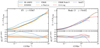 |
Fig. 1. Left panel: Comparisons between N-body simulations, e-Mantis and FORGE for |fR0| = 10−5. N-body data from simulations run by MG-AREPO and ECOSMOG codes are taken from the latest comparison project presented in Paper 1. We also include the prediction of FORGE where the cosmological parameters in the fiducial ΛCDM simulation, Ωm = 0.31315 and h = 0.6737, are used to make the prediction (FORGE Node 0). Right panel: Comparison of four prescriptions with an N-body simulation run by MG-AREPO. This simulation is one of the simulations used for training to construct the FORGE emulator (Node 13). The measurement of the power spectrum was done in Paper 2. |
To further investigate this issue with FORGE, we used the measurement of the power spectrum in one of the nodes in the FORGE simulation suite (Node 13) run by MG-AREPO that is closest to the Euclid reference cosmology that we will use in this paper with non-zero |fR0|. This simulation has the following cosmological parameters: Ωm = 0.34671, h = 0.70056 and σ8 = 0.78191 and we show a comparison at z = 0.652. Both ΛCDM and f(R) simulations with |fR0| = 10−4.90056 are available so that we can measure Ξ directly. We note that the pipeline developed in Paper 2 measures the power spectrum only up k = 3 h Mpc−1. In this case, both FORGE and e-Mantis agree with MG-AREPO within 1% up to k = 3 h Mpc−1. The fitting formula and ReACT agree with MG-AREPO within 1% up to k = 1 h Mpc−1. Given this result, the large discrepancy between FORGE and MG-AREPO is likely to be caused by emulation errors as well as calibrations using the halofitΛCDM power spectra predictions.
4.1.2. Comparison in the Euclid reference cosmology
In this paper, we consider the model called HS6 in Casas et al. (2023), which has the following parameters:
 (27)
(27)
The cosmological parameters are the same ones adopted in EC20. Casas et al. (2023) show that this value of |fR0| = 5 × 10⁻⁶ can be well constrained by the Euclid photometric probes. Also the range of |fR0| covered by the four models is wider than the errors predicted in Casas et al. (2023). Our fiducial cosmology includes massive neutrinos with a total mass of ∑mν = 0.06 eV, but we keep ∑mν fixed in the following analysis.
Figure 2 shows a comparison of the power spectrum and the angular power spectrum for WL, GCph and their cross-correlation XCph. In these plots, we show the ratio to the ΛCDM prediction and error bars from the diagonal part of the covariance matrix. For the power spectrum comparison at z = 0.5, we see that e-Mantis and fitting agree best. This is not surprising as these two predictions are based on N-body simulations ran by the same code ECOSMOG. On the other hand, FORGE overestimates Ξ at k = 0.1 h Mpc−1. This is similar to the deviation we find in the comparison with the N-body simulation from Paper 1 although the deviation is smaller, at the 2% level. This is likely due to the fact that Ωm in HS6 is closer to Ωm in the fiducial ΛCDMFORGE simulation (Ωm = 0.31315). On the other hand, ReACT underestimates Ξ at k < 0.1 h Mpc−1 and even predicts Ξ < 1. As we discussed in the previous section, we enforce Ξ ≥ 1.
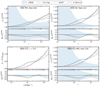 |
Fig. 2. Comparisons between all models considered for the HS6 fiducial cosmology for angular power spectra of WL (top left), galaxy clustering (top right) and their cross-correlation (bottom right) as well as for the matter power spectrum (bottom left). We show these for the WL redshift bin 6 and galaxy clustering bin 2, with the matter power spectrum plotted at z = 0.5, the redshift at which the kernels of both observables peak for the chosen bins. For all angular spectra, the error bands taken from the diagonal of the covariance are also shown. |
4.2. Forecasting errors and biases
4.2.1. Forecasting errors for WL
We first compared errors obtained by running MCMC using the synthetic data created by one of the four nonlinear models and fitting it by the same model. In this case, by definition, we recover the input parameters that were used to create the synthetic data. Our interests are constraints on the |fR0| parameter and cosmological parameters. We first considered the WL-only case. In this case, we imposed a tight Gaussian prior on the spectral index, ns, taken from the Planck results (Planck Collaboration VI 2020) and on the baryon density parameter, using Big Bang nucleosynthesis constraints (Pisanti et al. 2021):
 (28)
(28)
as we do not expect to obtain strong constraints on these parameters from WL alone. The parameters that are used in the MCMC runs are summarised in Table 5, including their fiducial values and prior ranges. As a convergence criterion, we used a Gelman–Rubin (Gelman & Rubin 1992) value of R − 1 < 0.01 for each individual sampling parameter using MontePython. For post-processing chains, we used GetDist8 (Lewis 2019).
Fiducial values and flat prior ranges for cosmological parameters, |fR0| and IA parameters.
Figure 3 shows the 2D contours of the constraints on parameters, and Table 6 and Table 7 summarise constraints on log10|fR0| for the optimistic and pessimistic settings. The constraints on cosmological parameters are consistent among the four different nonlinear models, while we see some notable differences in the constraints on |fR0|. In the case of the optimistic setting, e-Mantis gives the tightest constraints, which is also closer to Gaussian. The fitting formula agrees with e-Mantis for small log10|fR0| but has a weaker constraint for larger log10|fR0|. Constraints from FORGE agree with the fitting formula for large log10|fR0|, but give a weaker constraint for small log10|fR0|. The degeneracy between log10|fR0|, Ωc h2 and ln(1010As) also presents some notable differences. The degeneracy for larger log10|fR0| is different for the fitting formula when compared with e-Mantis and FORGE. This could be attributed to the fact that the fitting formula does not include any cosmological parameter dependence in the prediction for Ξ(k, z). We observe similar agreements and disagreements for the pessimistic setting, but the agreement among e-Mantis, FORGE and the fitting formula is better, particularly for small log10|fR0|. ReACT gives a weaker constraint on log10|fR0|, but the constraints on cosmological parameters are consistent among the four different models. This is due to the weak cosmology dependence of Ξ(k, z), as discussed in Winther et al. (2019), and the fact that the constraint on cosmological parameters is coming from the ΛCDM power spectrum, which is common in all these four models.
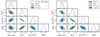 |
Fig. 3. Constraints on parameters where the same model is used to create the synthetic data and perform the fitting such that the input parameters are reproduced. Left panel: WL optimistic case. Right panel: WL pessimistic case. |
Mean, standard deviation, and 68.3% upper and lower limit of log10|fR0| for the WL optimistic setting
Mean, standard deviation, and 68.3% upper and lower limit of log10|fR0| for the WL pessimistic setting.
We compared the constraints from the MCMC analysis with the Fisher Matrix forecast and show this in Fig. 3. The MontePython pipeline can be used as a Fisher Matrix forecast tool (Casas et al. 2024), which was shown to agree very well with previous Fisher Matrix forecasts given by EC20. We note that in Casas et al. (2023), no prior was imposed on ns and Ωbh2, thus no direct comparison is possible. Instead, we used MontePython as a Fisher Matrix forecast tool and compared the result with the MCMC analysis to validate the Fisher Matrix forecast. To be consistent with Casas et al. (2023), we used the fitting formula as the nonlinear model. The 1σ error is very consistent: the Fisher Matrix forecast gives 0.111, while the MCMC analysis gives 0.116. The constraint from MCMC is non-Gaussian and the 1D posterior has a slightly longer tail for large log10|fR0|. The constraints on cosmological parameters agree very well between the Fisher Matrix forecast and the MCMC result.
4.2.2. Assessing biases for WL
Next, we created the synthetic data using FORGE and we fitted it by different nonlinear models to assess the biases in the recovered parameters due to the difference in the nonlinear modelling. We selected FORGE to create the data because it has a relatively narrow prior range for |fR0| and we encountered a problem with that range when using FORGE as the model to fit when including baryonic effects. We should note that FORGE has a larger discrepancy with other nonlinear models. As we discussed before, this could be attributed to emulation errors and calibration with halofit. In particular, this choice is disadvantageous to ReACT as the difference of the prediction for Ξ from FORGE is the largest. Thus, the estimation of bias in recovered parameters presented in this section is conservative, particularly for ReACT.
Figure 4 shows the 2D contours of the constraints on parameters, and Table 8 and Table 9 summarise constraints on log10|fR0| for the optimistic and pessimistic settings. We first start from the optimistic setting. Since ReACT is valid only up to k = 3 h Mpc−1, we did not include ReACT in this case. The fitting formula and e-Mantis recover the input parameters within 1σ. In the case of e-Mantis, cosmological parameters are well recovered, but there is a slight bias in the recovered log10|fR0|. On the other hand, a slight bias appears in h in the case of the fitting formula. This may be attributed to the fact that the fitting formula does not include cosmological parameter dependence in the prediction of Ξ. To quantify the bias, we define a 1D bias as
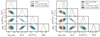 |
Fig. 4. Bias due to different nonlinear modelling. The synthetic data are created by FORGE and fitted by four different models. Left panel: WL optimistic case. Right panel: WL pessimistic case. |
 (29)
(29)
Mean, standard deviation, and 68.3% lower and upper limit of log10|fR0| for the optimistic setting.
Mean, standard deviation, and 68.3% lower and upper limit of log10|fR0| for the pessimistic setting.
where μ and σ are the mean and 1σ error computed from the 1D marginalised posteriors. If μ > μFORGE (μ < μFORGE), we use the upper (lower) 68.3% confidence interval to obtain σFORGE. The 1D bias for log10|fR0| is B1D = 0.273 and 0.602 for the fitting formula and e-Mantis, respectively.
We see a similar result in the pessimistic setting for e-Mantis and the fitting formula. In this case, the input log10|fR0| is well within 1σ although h is again slightly biased. The 1D bias for log10|fR0| is B1D = 0.441 and 0.518 for the fitting formula and e-Mantis, respectively, while the 1D bias for h is 0.988 and 0.812 for the fitting formula and e-Mantis, respectively. On the other hand, we find a bias in the recovered log10|fR0| when ReACT is used. As mentioned above, we should bear in mind that the choice of FORGE as a fiducial is disadvantageous for ReACT. In the case of ReACT, the difference from FORGE leads to biases also in the cosmological parameters leading to larger Ωch2 and smaller ln(1010As) and h. This is due to the different k dependence of Ξ between ReACT and FORGE and this is compensated by adjusting cosmological parameters as well as log10|fR0| leading to a stronger bias. The 1D bias for log10|fR0| reaches B1D = 3.11. We will discuss how to mitigate this bias by correcting the prediction for the fiducial cosmology and including theoretical errors in Sect. 6.
Since the FORGE prediction deviates from the other three models, we also performed the same analysis using e-Mantis as fiducial data for the pessimistic setting. We show the results in Appendix A. Qualitatively, we obtain consistent results. As we can see from Fig. A.1, the 2D contours overlap in the same way as the case where FORGE is used as fiducial, while the mean of log10|fR0| obtained by ReACT is closer to the input value. However, we still find that the 1D bias is at 3 sigma level due to the smaller errors of e-Mantis compared with FORGE.
4.2.3. 3 × 2 pt analysis
We considered the constraints from 3 × 2 pt statistics by adding GCph and its cross-correlation XCph to WL. In this paper, we use a simple model of the scale-independent linear bias as in ΛCDM. This assumption needs to be reexamined in f(R) gravity as the scale-dependent growth will lead to a scale-dependent bias. The effect of f(R) gravity on the halo bias was studied in simulations (Arnold et al. 2019b) and the anlytic model was developed by Valogiannis & Bean (2019). However, the linear bias assumption also needs to be relaxed even in ΛCDM and it is beyond the scope of this paper to implement a more complete bias description. For this reason, we consider the pessimistic case only and focus our attention on a comparison with the Fisher Matrix forecast and check if the bias when FORGE is used to create the data becomes worse with the increasing statistical power. We also do not include ReACT as we already observe a significant bias with WL only.
We have ten scale-invariant bias parameters, one for each redshift bin. For the 3 × 2 pt analysis, we vary ns, but we still impose a tight Gaussian prior on Ωb h2 as it is unlikely to get a tighter constraint than the Big Bang nucleosynthesis constraints.
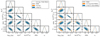 |
Fig. 5. Constraints from 3 × 2 pt analysis in the pessimistic setting. In the left panel, the same nonlinear model is used for the data and the fitting while in the right panel, the data are generated by FORGE. |
The parameters used in addition to the WL analysis are listed in Table 10. We did not change the fiducial bias parameters from EC20 as there is no prediction of the linear bias in f(R) gravity. The fiducial bias adopted in EC20 will need to be improved even in ΛCDM. Our prime focus is the study of the effect of nonlinear models and we vary the linear bias in the MCMC analysis resulting in different constraints depending on the nonlinear model used. The observed covariance was built from synthetic data. Thus the effect of f(R) gravity was included in the covariance. We independently checked that the constraints on parameters do not change by using the ΛCDM covariance. Thus we expect that the effect of f(R) on galaxy bias has also negligible effects on the covariance.
Additional parameters that are varied in the 3 × 2 pt analysis.
The left-hand side of Fig. 5 shows the 2D contours of the constraints on parameters, and Table 11 summarises constraints on log10|fR0| where the same nonlinear model is used for the data and the model. The right-hand side of Fig. 5 shows the 2D contours of the constraints on parameters, and Table 12 summarises constraints on log10|fR0| as well as 1D bias for log10|fR0| when FORGE is used to create the data.
Mean, standard deviation, and 68.3% lower and upper limit of log10|fR0| for the 3 × 2 pt pessimistic setting.
Mean, standard deviation, and 68.3% lower and upper limit of log10|fR0| for the 3 × 2 pt pessimistic setting
In the case where the same nonlinear model is used for the data and the model, errors are consistent between the fitting formula and e-Mantis, although we still observe the same longer tail for larger log10|fR0| for the fitting formula as we observe for WL. FORGE gives slightly tighter constraints on log10|fR0|. Constraints on cosmological parameters are very consistent among the three different nonlinear models. The Fisher Matrix forecast using the fitting formula is also very consistent with the MCMC results. We note that errors from 3 × 2 pt analysis in the pessimistic setting are comparable to or better than WL alone in the optimistic setting. This demonstrates the strength of the 3 × 2 pt analysis although we should bear in mind the limitation of the bias model used in this analysis.
We find that the increased statistical power does not degrade the agreement between FORGE and e-Mantis. When FORGE is used to create the data, the input parameters are well recovered by e-Mantis, although h is slightly biased as in the WL-only case. The 1D bias for log10|fR0| is given by 0.150. In the case of the fitting formula, the bias in cosmological parameters becomes worse compared with WL. This could be attributed to the fact that the fitting formula does not take into account the cosmological parameter dependence of Ξ as mentioned before. The 1D bias for log10|fR0| also becomes slightly larger, with a value of B1D = 0.667.
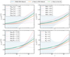 |
Fig. 6. Effect of log10|fR0|, two baryonic parameters log10Mc and θej, and h on the WL angular power spectrum in bin 10. The dotted lines show predictions of e-Mantis with varying these parameters individually. The plot shows the ratio to the ΛCDM power spectrum. The plot includes the prediction of FORGE and e-Mantis with the fiducial parameters and the e-Mantis prediction using the best-fit values (log10|fR0| = −5.765, 100h = 65.736, log10(Mc) = 12.999) with the data created by FORGE. We can see that the e-Mantis prediction can fit the FORGE by adjusting these parameters. We note that the cosmological parameters for the ΛCDM power spectrum, |

5. Baryonic effects
5.1. Adding baryonic effects using BCemu
In this section, we study the impact of baryonic effects on the constraints on the f(R) parameter. We use the seven-parameter emulator of baryonic effects called BCemu (Giri & Schneider 2021) and we assume that the baryonic effects and the modified gravity effects can be treated independently as discussed in Sect. 3 (Arnold & Li 2019). The BCemu parameters govern the gas profiles and stellar abundances in haloes. It is not our intention to study in detail the baryonic effects. We use the default values for the baryonic parameters provided with BCemu and use the full prior range. We choose not to include any redshift dependence. This is because we need to impose a tight prior range for these parameters at z = 0 to keep them within the prior range and we may miss important degeneracies between baryonic parameters and log10|fR0|. We found that two baryonic parameters,  and θej, have the strongest effects on the matter power spectrum and they are well constrained in the presence of the f(R) parameter. Thus, we only vary these two parameters. In BCemu, the gas profile is modelled as a cored double power law.
  controls the dark matter halo mass dependence of the logarithmic slope of the first-cored power law. It allows the profile to become less steep than the Navarro et al. (1996) one for
  . The parameter θej determines the scale radius (with respect to the virial radius) of the second-cored power law. Table 13 summarises the fiducial values and priors for baryonic parameters. We will use the dimensionless parameter Mc that is related to the one defined in Giri & Schneider (2021) via
  where M⊙ is the solar mass.
Fiducial values and priors for BCemu parameters.
5.2. Effects of adding baryons
Figure 6 shows the effect of changing log10|fR0|, h, and two baryonic parameters on the ratio of the WL angular power spectrum to the ΛCDM one. Baryonic effects introduce scale-dependent modifications to the angular power spectrum that are similar to the effect of f(R) at ℓ > 100. On the other hand, h changes the overall amplitude of the angular power spectrum as it changes Ωm. We will see that the interplay between these parameters leads to interesting degeneracies.
Figure 7 shows the 2D contours of the WL constraints on parameters for the optimistic settings with baryons and Table 14 summarises constraints on log10|fR0|. In the case of the optimistic setting, when e-Mantis is used as the data and the model, the two baryonic parameters degrade the constraints on log10|fR0|: the 1σ error becomes 0.281 while it was 0.088 without baryons. However, it is important to stress that log10|fR0| and the two baryonic parameters are still constrained well within the prior range of these parameters. It means that the impact of modified gravity on the high-k tail of the matter power spectrum is not washed out by the baryonic feedback, and we can still distinguish between the effect of f(R) and baryons.
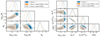 |
Fig. 7. Constraints on parameters from the WL optimistic setting with baryons. We show the case where e-Mantis is used to create both the data and fitting and the case where FORGE is used to create the data and it is fitted by e-Mantis. We also include the case where we impose a Gaussian prior on log10 Mc with the width of 0.2 in the case of FORGE fiducial data. Left panel: Constraints on baryonic parameters. Right panel: Constraints on cosmological parameters. |
Mean, standard deviation, and 68.3% lower and upper limit of log10|fR0| for the WL optimistic setting with baryons.
Nevertheless, if FORGE is used as the data, the difference between FORGE and e-Mantis in the matter power spectrum can be absorbed by the shift in log10Mc and h, and the constraint on log10|fR0| is shifted along the degeneracy direction between log10|fR0| and log10Mc as well as h. This can be understood from Fig. 6. The difference of the scale dependence between e-Mantis and FORGE at ℓ > 100 can be adjusted by decreasing log10|fR0| and decreasing log10Mc. This leads to a lower amplitude that can be adjusted by decreasing h. Due to the combination of these effects, the best-fit log10|fR0| becomes smaller. We note that e-Mantis does not include the h dependence in the prediction for Ξ(k, z) explicitly, but it depends on h implicitly through σ8ΛCDM. However, this dependence of h on Ξ(k, z) is very weak. To compute the power spectrum in f(R) we use Pf(R) = Ξ(k, z)PΛCDM(k, z). The e-Mantis emulator provides us with the first factor, Ξ(k, z), and a ΛCDM emulator provides the last factor. The h dependence comes from the ΛCDM power spectrum not from Ξ(k, z).
As a result, we obtain a 95.5% upper limit of log10|fR0| as log10|fR0| < −5.477, which is incompatible with the input value of log10|fR0| = −5.301. This is partly due to prior volume effects shifting the contour to lower values of log10|fR0|, caused by the strong degeneracy between log10|fR0| and log10Mc, as well as h.
To confirm this, we obtain a profile likelihood for log10|fR0| by fixing log10|fR0| and finding a minimum χ2 by varying other parameters. The profile likelihood was obtained by PROSPECT9 (Holm et al. 2024). This is shown in Fig. 8. The global best-fit value for log10|fR0| is obtained as log10|fR0| = −5.765, which is larger than the mean of the 1D marginalised posterior log10|fR0| = −6.087. Figure 6 also shows the prediction of e-Mantis with the best-fit values, which agrees well with FORGE. The Δχ2 for the input value of log10|fR0| = −5.301 is found as Δχ2 = 2.657, thus it is still within 2σ. We also observe that the Δχ2 curve becomes flat for smaller values of log10|fR0|.
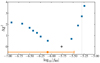 |
Fig. 8. Profile likelihood for log10|fR0| where FORGE is used to create data fitted by e-Mantis with baryons in the optimistic setting of WL. The square points show Δχ2 from the best-fit indicated by a diamond. The 95.5% confidence interval from the 1D marginalised posterior is shown as the error bar. The vertical dotted line indicates the input value of −log10|fR0| = 5.301. We see that the 1D marginalised posterior is shifted to smaller values of log10|fR0|. |
We also tested the fitting formula as a model to fit to the data generated by FORGE. In this case, the posterior is highly non-Gaussian and the chains did not converge well.
This implies that we can break the degeneracy between f(R) gravity and baryonic effects, but we need to have an accurate nonlinear model for the f(R) gravity model. Otherwise, we could obtain a significantly biased result in terms of the 1D marginalised constraint. We note that if we have a physical prior on log10Mc from baryonic physics, we could break the degeneracy between log10|fR0| and log10Mc. For example, in the case where FORGE was used as the data and they were modelled by e-Mantis, the mean of log10Mc is significantly shifted to a smaller value as we can see in Fig. 7. If we had a prior on log10Mc to prevent this, this bias could be avoided. To test this idea, we also ran an analysis imposing a prior on log10Mc and showed the result in Fig. 7. We used a Gaussian prior with the width of 0.2, which was estimated from the WL informed gas and stellar mass fraction measurements of massive haloes by Grandis et al. (2024). This prior is consistent with the error on log10Mc that we obtained by using e-Mantis both for data and model. We observe that the bias is relaxed slightly; however, the degeneracy between log10Mc and log10|fR0| is quite strong and this prior is not enough to alleviate the bias in the marginalised constraints. An improved prior from external data is needed to fully break this degeneracy.
We assumed that the effect of f(R) gravity and baryonic effect can be treated independently. Recently, the coupling between baryonic feedback and cosmology has been studied showing that the combined effect of baryonic and non-baryonic suppression mechanisms is greater than the sum of its parts for decaying dark matter (Elbers 2025). The effect of this coupling on the degeneracy needs to be studied in the future.
Next, we consider the pessimistic setup. Figure 9 shows the 2D contours of the WL constraints on parameters for the optimistic settings with baryons and Table 15 summarises constraints on log10|fR0|. In this case, due to the weaker constraining power, the 99.7% confidence level upper bound on log10|fR0| reaches the prior boundary of log10|fR0| = −7. Also, the 95.5% confidence level upper bound of θej is bounded by the prior. If the data are generated by FORGE, strong degeneracies appear among log10|fR0| and two baryonic parameters. The input log10|fR0| is consistent within 1σ for the fitting formula and e-Mantis although the prior bound log10|fR0| = −7 is reached at 95.5% confidence level lower bound. On the other hand, for ReACT, the input value is outside the 95.5% confidence level upper bound. As we already observed without baryons, h is biased to a lower value.
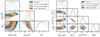 |
Fig. 9. Constraints on parameters from the WL pessimistic setting with baryons. As in Fig. 7, we show the case where e-Mantis is used to create both the data and fitting as well as the case where FORGE is used to create the data and it is fitted by e-Mantis, ReACT and the fitting formula. Left panel: Constraints on baryonic parameters. Right panel: Constraints on cosmological parameters. |
Mean, standard deviation, and 68.3% lower and upper limit of log10|fR0| for the WL pessimistic setting with baryons.
We also checked the case where fiducial data is generated by e-Mantis. As we can see in Fig. A.2, unlike the case without baryons, the agreements between e-Mantis, fitting and ReACT are improved significantly compared with the case where FORGE is used for fiducial data. Particularly, for ReACT, the mean of log10|fR0| is now consistent with the input value within 1σ.
5.3. Constraints on |fR0| with the ΛCDM data
Based on these results, we consider the pessimistic setting and use e-Mantis to obtain an upper limit of log10|fR0| in the presence of baryonic effects to be conservative. Figure 10 shows the 2D contours of the WL constraints on parameters for the pessimistic settings where ΛCDM is used to create the data. We find that the recovered cosmological parameters are consistent with the input values. The mean of 1D marginalised constraints of baryonic parameters are slightly biased due to the strong degeneracy between them, but it is still consistent within 1σ. We obtain the 95.5% confidence level upper bound on log10|fR0| as
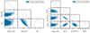 |
Fig. 10. Constraints on parameters from the WL pessimistic setting with baryons where the data are created in ΛCDM and it is fitted by e-Mantis. Left panel: Constraints on baryonic parameters. Right panel: Constraints on cosmological parameters. |
 (30)
(30)
We note that this bound depends on the prior log10|fR0| = −7. To obtain the prior-independent bound, we follow the approach presented in Gordon & Trotta (2007), Piga et al. (2023) and Kou et al. (2024). The ratio of the marginalised posterior and prior is given by
 (31)
(31)
where x is the parameter we are interested in (i.e. log10|fR0|), d is the data, p is the prior, and 𝒫 is the posterior. The Bayes factor, B(x1, x2), which quantifies the support of the models with x = x1 over the models with x = x2, is given by
 (32)
(32)
where ℒ(d ∣ x) is the marginalised likelihood of the data for parameter x. For our purpose, we chose x = log10|fR0| and fixed x1 to be the upper bound of the prior, x1 = −7. Following Gordon & Trotta (2007), we then used B(x1, x2) = 2.5 to find x2 so that the model with x = x1 is favoured compared to the model with x = x2 at 95.5% confidence level. This gives the 95.5% confidence interval of log10|fR0| that does not depend on the prior. We note that this method applies only to a ℒ(d ∣ x) that is a monotonic function of x. Employing this technique, we obtain
 (33)
(33)
Finally, in Fig. 11, we present the constraints on Ωm and log10|fR0| so that we can compare these with those in the literature (Schneider et al. 2020; Harnois-Déraps et al. 2023; Spurio Mancini & Bose 2023). It is not possible to make a direct comparison due to various differences in the setting. Nonetheless, our constraint is comparable to the one presented in Schneider et al. (2020) [log10|fR0| < −5.3] where a similar analysis was done by combining BCemu and the fitting formula. We cannot also make a comparison with Harnois-Déraps et al. (2023) as baryonic effects are not included in their analysis, but again the constraint is comparable [log10|fR0| < −5.24]. On the other hand, our constraint is much weaker than the one found in Spurio Mancini & Bose (2023) that used ReACT with BCemu. We refer the readers to Spurio Mancini & Bose (2023) for possible explanations. In our analysis, ReACT tended to prefer a lower value of log10|fR0| when FORGE is used as data and this might be one of the reasons for this difference. Finally, a recent study by Tsedrik et al. (2024) used similar settings to forecast cosmic shear constraints on model-independent parametrisations of modified gravity theories with scale-independent linear growth. They found that a much better understanding of baryonic feedback is needed in order to detect a screening transition.
6. Theoretical error
Any theoretical prediction will in general come with an associated error and should be included in the likelihood if it is not subdominant to the statistical error. In this section, we discuss the implementation of theoretical errors in our pipeline. To be conservative, we estimated the theoretical errors using ReACT and FORGE as these two give the most discrepant results. We applied this method to ReACT for the pessimistic case of WL to check if we could remove the parameter biases that we observe for the data created by FORGE at the expense of enlarging error bars.
6.1. Adding uncorrelated theoretical errors to the likelihood
The implementation presented in this work is based on the work of Audren et al. (2013). We have adjusted the recipe to the full 3 × 2 pt likelihood, although we only show the result for the WL analysis in this paper. Here, we discuss the idea behind the formulation. We calculated the angular power spectrum from the power spectrum using Eq. (1). If there is some uncertainty in the modelling of the nonlinear power spectrum, this propagates to the angular power spectrum. As Eq. (1) is a linear functional of the nonlinear matter power spectrum, ℱ[Pδδ], we can propagate the error on the power spectrum, ΔPδδ, and find
![Mathematical equation: $$ \begin{aligned} \mathcal{F} [P_{\delta \delta }+\Delta P_{\delta \delta }] = \mathcal{F} [P_{\delta \delta }] + \mathcal{F} [\Delta P_{\delta \delta }] C_{ij}^{XY}(\ell ) + E_{ij}^{XY}(\ell ), \end{aligned} $$](/articles/aa/full_html/2025/06/aa52184-24/aa52184-24-eq61.gif) (34)
(34)
where we have defined the angular power spectrum error,  . Following Audren et al. (2013), we defined the relative error on the power spectrum:
 (35)
(35)
We took the most conservative approach and assumed that the error is uncorrelated between different values of ℓ. To account for this uncorrelated theoretical error, we added a new nuisance parameter, εℓ, for each multipole and define the shifted covariance as
 (36)
(36)
The free parameters, εℓ, have the following meaning: they quantify how many standard deviations the shifted covariance matrix is from the theoretically predicted one. We treat them as a random Gaussian variable with zero mean and a standard deviation of one. The normalisation factor, L1/2, where L = ℓmax − ℓmin + 1, will become clear soon. The log-likelihood function becomes
![Mathematical equation: $$ \begin{aligned} \tilde{\chi }^2 \left(\varepsilon _\ell \right) = \sum _{\ell =\ell _{\mathrm{min} }}^{\ell _{\mathrm{max} }} \left[ (2\ell +1) f_{\rm sky} \left( \frac{\tilde{d}^\mathrm{mix}_\ell \left(\varepsilon _\ell \right)}{\tilde{d}^\mathrm{th}_\ell \left(\varepsilon _\ell \right)} + \ln { \frac{ \tilde{d}^\mathrm{th}_\ell \left(\varepsilon _\ell \right)}{d^\mathrm{obs}_\ell }}-N\right) + \varepsilon _\ell ^2\ \right]. \end{aligned} $$](/articles/aa/full_html/2025/06/aa52184-24/aa52184-24-eq65.gif) (37)
(37)
The quantities  and
and  are constructed in the same way as dth and dmix [see Eqs. (15) to (17)] using the shifted covariance matrix
  . To include the theoretical error, we vary εℓ and marginalise over them. To a very good approximation, this is equivalent to minimising the
  with respect to εℓ at the level of the likelihood. Thus, we define our new χ2 as the minimum of the
  with respect to εℓ:
 (38)
(38)
The normalisation factor, L1/2, can be explained as follows. If we were to measure  , the minimisation would find εℓ = L−1/2. The resulting χ2 = ∑ℓεℓ2 = ∑ℓL−1 = 1 would match our expectation that a one-sigma theoretical error for each ℓ results in an increase in χ2 by one.
The main ingredient of this formulation is the relative error function α(k, z) defined in Eq. (35). The construction of α(k, z) using FORGE and ReACT will be discussed in Appendix B.
6.2. Numerical implementation
The numerical computation of the theory error covariance  follows the prescription presented by Casas et al. (2024). For the minimisation, we can use the fact that all the free εℓ are independent of each other, and we can do the minimisation for each multipole separately. We use Newton’s method to find the minimum. For this, we have to compute the first and second derivatives of the likelihood with respect to εℓ. For any single multipole, we find
 (39)
(39)
The derivatives of the determinants are computed using Jacobi’s formula. This gives, for example
![Mathematical equation: $$ \begin{aligned} \left(\tilde{d}^\mathrm{th} _\ell \right)\prime = \det \left( \hat{C}_\ell ^\mathrm{th} \right)\,L^{1/2}\,\mathrm{Tr}\left[ \left(\hat{C}_\ell ^\mathrm{th} \right)^{-1} \, E_\ell \right], \end{aligned} $$](/articles/aa/full_html/2025/06/aa52184-24/aa52184-24-eq75.gif) (40)
(40)
and a similar expression for  . We compute the inverse of the covariance numerically and obtain the second derivatives numerically from the first derivative by doing a double-sided three-point stencil. The minimisation would then need to be done for each multipole. For the pessimistic settings, this would correspond to a minimisation in a 1500-dimensional parameter space. To save time, we only do the minimisation on a logarithmically-spaced grid with 100 discrete values. The other values are obtained from an interpolating function. We checked that the effect of the interpolation does not change the results by more than 1%. The obtained εℓ tend to vary continuously with ℓ, as they try to mimic the effects of changing other theory parameters to the observed power spectrum.
6.3. Application to ReACT
We first applied this method to the case in which the data are created by FORGE and the parameter fitting is done by ReACT. Due to the significant bias in the recovered parameters for both |fR0| and cosmological parameters, we find that the inclusion of theoretical errors is not enough to mitigate the bias. Therefore, we additionally correct the prediction of ReACT by FORGE for the fiducial cosmology as
 (41)
(41)
The constraints on cosmological parameters are shown in the left panel of Fig. 12. In this case, as expected, we recover the input parameters in an unbiased way when the data are created by FORGE. We see that theoretical errors affect mainly log10|fR0| and h. In order to check a non-trivial case, next we create the data with e-Mantis. The result is shown in the right panel of Fig. 12. Without theoretical errors, the means of 1D marginalised constraints for log10|fR0|, Ωch2, and ln(1010As) are slightly biased compared with the input values. The inclusion of the theoretical errors largely resolves these biases not only by enlarging the error bars but also by making the means closer to the input values. We note that the inclusion of theoretical errors in this case is important to justify the rescaling of Ξ in Eq. (41). We also note that the theoretical error included here overestimates the errors significantly now that we corrected the prediction of ReACT by FORGE for the fiducial cosmology.
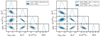 |
Fig. 12. Effect of adding theoretical errors. Left panel: Data are created by FORGE in the WL pessimistic setting and fitted by ReACT corrected by FORGE for fiducial cosmology, Eq. (41), with and without theoretical errors. Right panel: Data are created by e-Mantis in this case. |
Finally, we study the impact of adding baryonic effects in the presence of theoretical errors. We again use e-Mantis as the data. The result is shown in Fig. 13. Due to the enlarged errors, constraints on parameters are not affected significantly by baryonic effects. Also, the means of the 1D marginalised constraint remain consistent with the input parameters. However, the inclusion of the theoretical errors changes the degeneracies between cosmological parameters, baryonic parameters and log10|fR0|. This leads to a tighter lower bound on log10|fR0| compared with the case where the same data are fitted by e-Mantis itself. This reinforces our conclusion that the 1D marginalised constraint on log10|fR0| is sensitive to degeneracies among parameters, and the difference in the theoretical predictions strongly affects the constraint.
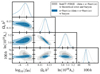 |
Fig. 13. Effect of adding theoretical errors in the presence of baryonic effects. Data are created by e-Mantis and fitted by ReACT corrected by FORGE for the fiducial cosmology with theoretical errors. For a comparison, we also show the result obtained by using e-Mantis to fit the same data. |
The result shown here is just an illustration of the inclusion of theoretical errors and their effects on the parameter constraints. Our implementation is flexible and it can be applied to any theoretical error described by the relative error function α(k, z) defined in Eq. (35).
7. Conclusion
In this paper, we have studied the effect of using different nonlinear predictions for the dark matter power spectrum on the parameter constraints in the Hu–Sawikci f(R) gravity model obtained from Euclid primary photometric probes. We implemented four different models in the MontePython pipeline to predict angular power spectra for WL, photometric galaxy clustering (GCph) and their cross-correlation (XCph). Comparing with the N-body simulation data obtained in Paper 1, we found that e-Mantis agrees very well with ECOSMOG, which was used to run simulations to construct the emulator, while FORGE had larger errors compared with the MG-AREPO simulation. The agreement is better for one of the N-body simulations used to construct FORGE obtained in Paper 2 run by MG-AREPO. This indicates that the difference between e-Mantis and FORGE is larger than the one in the baseline N-body simulations (i.e. ECOSMOG and MG-AREPO) mainly due to the way FORGE was constructed. In the Euclid reference cosmology, FORGE gives a larger Ξ, the ratio between the power spectrum in f(R) and in ΛCDM, on all scales compared with e-Mantis and the fitting formula at the 2% level. ReACT underestimates Ξ compared with FORGE more than e-Mantis and the fitting formula at intermediate k.
We used the fiducial value of |fR0| = 5 × 10⁻⁶ (log10|fR0| = −5.301) and ran MCMC in the Euclid fiducial cosmology defined in EC20. For the fitting formula, the Fisher Matrix forecast and MCMC results generally agree well although the MCMC result is non-Gaussian. This is partly caused by a lack of cosmological parameter dependence of Ξ, which affects the degeneracy between log10|fR0| and cosmological parameters for large log10|fR0|. e-Mantis gives more Gaussian constraints with smaller errors. When FORGE is used to create the data, the 1D mean of log10|fR0| is not strongly biased in the case of e-Mantis and the fitting formula and the 1D bias is at most 0.6σ. Even for the 3 × 2 pt analysis including all the probes and their cross-correlations, the 1D bias is 0.15σ for log10|fR0| in the case of e-Mantis.
The impact of baryonic physics on WL was studied by using a baryonification emulator BCemu. For the optimistic setting, the f(R) parameter and two main baryonic parameters are well constrained despite the degeneracies among these parameters. However, the difference in the nonlinear dark matter prediction can be compensated by the adjustment of baryonic parameters as well as cosmological parameters, and the 1D marginalised constraint on log10|fR0| is biased. This bias can be avoided in the pessimistic setting at the expense of weaker constraints. For the pessimistic setting, using the ΛCDM synthetic data for WL, we obtained the prior-independent bound of log10|fR0| < −5.6 using e-Mantis.
ReACT shows a large bias in log10|fR0| as well as cosmological parameters when FORGE was used to create the data. This is because the prediction of ReACT is furthest away from FORGE. We implemented a method to include uncorrelated theoretical errors proposed in Audren et al. (2013) to address this issue. The method is based on the relative error function for the nonlinear dark matter power spectrum. We estimated this using the difference between FORGE and ReACT. We found that the inclusion of theoretical errors alone was not enough to mitigate the bias. We then corrected the prediction of ReACT with FORGE for the fiducial model. We applied this model to the data created by e-Mantis. We found that theoretical errors, in this case, helped reduce the bias not only by enlarging errors but also by making the means of 1D marginalised constraint closer to the input values. When we added baryonic effects with BCemu, errors were not significantly affected and the input values were still recovered. However, the lower bound on log10|fR0| is tighter than the one obtained by applying e-Mantis itself. This reinforces our conclusion that the 1D marginalised constraint on log10|fR0| is sensitive to the degeneracies among parameters.
Based on the result of this paper, we draw the following conclusions:
-
It is important to check the agreement of different N-body codes that are used to create theoretical predictions. This means not only the code itself, but also accuracy settings. In Paper 1, we found that the accuracy setting such as the refinement criteria in the adaptive mesh refinement method has a large effect on the power spectrum. With the controlled accuracy setting, it is possible to realise 1% agreements between different N-body codes in terms of Ξ(k, z) in the Hu–Sawicki f(R) gravity model.
-
We then need to check the accuracy of emulators. We found that FORGE suffers from larger emulation errors and this leads to a larger difference between FORGE and e-Mantis compared with the difference in their baseline N-body code MG-AREPO and ECOSMOG in some cosmologies. Improving the emulation technique will make the agreement better.
-
Including baryonic effects can worsen the bias in the 1D marginalised constraint on log10|fR0|. This is because the difference in the nonlinear dark matter power spectrum prediction can be compensated by the adjustment of baryonic parameters, and the best-fit values are biased. In addition, the degeneracy between baryonic parameters, cosmological parameters and log10|fR0| leads to a stronger volume effect. This bias can be avoided if there is a prior on baryonic parameters from external datasets for example.
-
To account for the uncertainty in the theoretical prediction for the nonlinear power spectrum, it is safer to include theoretical errors. In this paper, we used a conservative error estimation using FORGE and ReACT. An improvement in emulators will make the theoretical error smaller, leading to better constraints. However, we still need to check whether or not the inclusion of baryons will change this conclusion.
The pipeline developed in this paper can be used to test the readiness of the nonlinear power spectrum prediction for the application to real data from Euclid in other extended cosmologies. For the Data Release 1 of Euclid and future data releases, we plan to improve the FORGE emulator and make the pipeline ready for the data analysis. We also plan to extend the analysis to the models studied in Frusciante (2024).
Finally, we note that our forecasts have ignored observational systematics such as shear and redshift measurement biases. For Stage-IV surveys like Euclid it is known that these need to be very well characterised in order to get accurate cosmological parameter estimates. This is a challenge that needs to be addressed for both ΛCDM and exotic cosmologies. A detailed study of this issue is beyond the scope of our paper, but we refer to Euclid Collaboration: Mellier et al. (2025) for details. In summary, the mean galaxy redshifts within the bins need to be known with an accuracy better than ∼0.002(1 + z) if errors in cosmological parameters are not to be degraded. On the other hand, Spurio Mancini & Bose (2023) included a parameter that shifts the mean of the redshift distribution in each redshift bin and found that these parameters are not strongly degenerate with the f(R) parameter.
Acknowledgments
The Euclid Consortium acknowledges the European Space Agency and a number of agencies and institutes that have supported the development of Euclid in particular the Agenzia Spaziale Italiana, the Austrian Forschungsförderungsgesellschaft funded through BMK, the Belgian Science Policy, the Canadian Euclid Consortium, the Deutsches Zentrum für Luft- und Raumfahrt, the DTU Space and the Niels Bohr Institute in Denmark, the French Centre National d’Etudes Spatiales, the Fundação para a Ciência e a Tecnologia, the Hungarian Academy of Sciences, the Ministerio de Ciencia, Innovación y Universidades, the National Aeronautics and Space Administration, the National Astronomical Observatory of Japan, the Netherlandse Onderzoekschool Voor Astronomie, the Norwegian Space Agency, the Research Council of Finland, the Romanian Space Agency, the State Secretariat for Education, Research, and Innovation (SERI) at the Swiss Space Office (SSO), and the United Kingdom Space Agency. A complete and detailed list is available on the Euclid web site (www.euclid-ec.org). K. K. is supported by STFC grant ST/W001225/1. B. B. is supported by a UK Research and Innovation Stephen Hawking Fellowship (EP/W005654/2). A. P. is a UKRI Future Leaders Fellow [grant MR/X005399/1]. P. C. is supported by grant RF/ERE/221061. M. C. acknowledges the financial support provided by the Alexander von Humboldt Foundation through the Humboldt Research Fellowship program, as well as support from the Max Planck Society and the Alexander von Humboldt Foundation in the framework of the Max Planck-Humboldt Research Award endowed by the Federal Ministry of Education and Research. F. P. acknowledges partial support from the INFN grant InDark and the Departments of Excellence grant L.232/2016 of the Italian Ministry of University and Research (MUR). FP also acknowledges the FCT project with ref. number PTDC/FIS-AST/0054/2021. GR’s research was supported by an appointment to the NASA Postdoctoral Program administered by Oak Ridge Associated Universities under contract with NASA. GR was supported by JPL, which is run under contract by the California Institute of Technology for NASA (80NM0018D0004). Numerical computations were done on the Sciama High Performance Compute (HPC) cluster which is supported by the ICG, SEPNet, and the University of Portsmouth. This work has made use of the Infinity Cluster hosted by Institut d’Astrophysique de Paris. We acknowledge open libraries support IPython (Perez & Granger 2007), Matplotlib (Hunter 2007), Numpy (Walt et al. 2011), and SciPy (Virtanen et al. 2020). For the purpose of open access, we have applied a Creative Commons Attribution (CC BY) licence to any Author Accepted Manuscript version arising. Supporting research data are available on reasonable request from the corresponding author.
References
- Albrecht, A., Bernstein, G., Cahn, R., et al. 2006, ArXiv e-prints [arXiv:astro-ph/0609591] [Google Scholar]
- Angulo, R. E., Zennaro, M., Contreras, S., et al. 2021, MNRAS, 507, 5869 [NASA ADS] [CrossRef] [Google Scholar]
- Arnold, C., & Li, B. 2019, MNRAS, 490, 2507 [NASA ADS] [CrossRef] [Google Scholar]
- Arnold, C., Leo, M., & Li, B. 2019a, Nat. Astron., 3, 945 [Google Scholar]
- Arnold, C., Fosalba, P., Springel, V., Puchwein, E., & Blot, L. 2019b, MNRAS, 483, 790 [NASA ADS] [CrossRef] [Google Scholar]
- Arnold, C., Li, B., Giblin, B., et al. 2022, MNRAS, 515, 4161 [CrossRef] [Google Scholar]
- Audren, B., Lesgourgues, J., Bird, S., Haehnelt, M. G., & Viel, M. 2013, JCAP, 01, 026 [CrossRef] [Google Scholar]
- Baldi, M., Villaescusa-Navarro, F., Viel, M., et al. 2014, MNRAS, 440, 75 [NASA ADS] [CrossRef] [Google Scholar]
- Bose, S., Li, B., Barreira, A., et al. 2017, JCAP, 02, 050 [Google Scholar]
- Bose, B., Cataneo, M., Tröster, T., et al. 2020, MNRAS, 498, 4650 [Google Scholar]
- Bose, B., Wright, B. S., Cataneo, M., et al. 2021, MNRAS, 508, 2479 [NASA ADS] [CrossRef] [Google Scholar]
- Bose, B., Tsedrik, M., Kennedy, J., et al. 2023, MNRAS, 519, 4780 [NASA ADS] [CrossRef] [Google Scholar]
- Brax, P., van de Bruck, C., Davis, A.-C., & Shaw, D. J. 2008, Phys. Rev. D, 78, 104021 [CrossRef] [Google Scholar]
- Brax, P., Casas, S., Desmond, H., & Elder, B. 2021, Universe, 8, 11 [NASA ADS] [CrossRef] [Google Scholar]
- Buchdahl, H. A. 1970, MNRAS, 150, 1 [NASA ADS] [Google Scholar]
- Burrage, C., March, B., & Naik, A. P. 2024, JCAP, 04, 004 [NASA ADS] [Google Scholar]
- Carrilho, P., Carrion, K., Bose, B., et al. 2022, MNRAS, 512, 3691 [Google Scholar]
- Carrion, K., Carrilho, P., Spurio Mancini, A., Pourtsidou, A., & Hidalgo, J. C. 2024, MNRAS, 532, 3914 [Google Scholar]
- Casas, S., Cardone, V. F., Sapone, D., et al. 2023, ArXiv e-prints [arXiv:2306.11053] [Google Scholar]
- Casas, S., Lesgourgues, J., Schöneberg, N., et al. 2024, A&A, 682, A90 [NASA ADS] [CrossRef] [EDP Sciences] [Google Scholar]
- Cataneo, M., Lombriser, L., Heymans, C., et al. 2019, MNRAS, 488, 2121 [Google Scholar]
- Cautun, M., Paillas, E., Cai, Y.-C., et al. 2018, MNRAS, 476, 3195 [NASA ADS] [CrossRef] [Google Scholar]
- Clifton, T., Ferreira, P. G., Padilla, A., & Skordis, C. 2012, Phys. Rep., 513, 1 [NASA ADS] [CrossRef] [Google Scholar]
- Desmond, H., & Ferreira, P. G. 2020, Phys. Rev. D, 102, 104060 [NASA ADS] [CrossRef] [Google Scholar]
- Elbers, W., et al. 2025, MNRAS., 537, 2160 [Google Scholar]
- Euclid Collaboration (Blanchard, A., et al.) 2020, A&A, 642, A191 [NASA ADS] [CrossRef] [EDP Sciences] [Google Scholar]
- Euclid Collaboration (Knabenhans, M., et al.) 2021, MNRAS, 505, 2840 [NASA ADS] [CrossRef] [Google Scholar]
- Euclid Collaboration (Bose, B., et al.) 2024, A&A, 689, A275 [Google Scholar]
- Euclid Collaboration (Sciotti, D., et al.) 2024, A&A, 691, A318 [NASA ADS] [CrossRef] [EDP Sciences] [Google Scholar]
- Euclid Collaboration (Adamek, J., et al.) 2025, A&A, 695, A230 [Google Scholar]
- Euclid Collaboration (Mellier, Y., et al.) 2025, A&A, 697, A1 [Google Scholar]
- Euclid Collaboration (Racz, G., et al.) 2025, A&A, 695, A232 [Google Scholar]
- Ferreira, P. G. 2019, ARA&A, 57, 335 [Google Scholar]
- Fiorini, B., Koyama, K., & Baker, T. 2023, JCAP, 12, 045 [NASA ADS] [Google Scholar]
- Frusciante, N., et al. 2024, A&A, 690, A133 [NASA ADS] [CrossRef] [EDP Sciences] [Google Scholar]
- Gelman, A., & Rubin, D. B. 1992, Statist. Sci., 7, 457 [NASA ADS] [Google Scholar]
- Giocoli, C., Baldi, M., & Moscardini, L. 2018, MNRAS, 481, 2813 [Google Scholar]
- Giri, S. K., & Schneider, A. 2021, JCAP, 12, 046 [CrossRef] [Google Scholar]
- Gordon, C., & Trotta, R. 2007, MNRAS, 382, 1859 [CrossRef] [Google Scholar]
- Grandis, S., Arico’, G., Schneider, A., & Linke, L. 2024, MNRAS, 528, 4379 [NASA ADS] [CrossRef] [Google Scholar]
- Guillet, T., & Teyssier, R. 2011, J. Comput. Phys., 230, 4756 [Google Scholar]
- Harnois-Déraps, J., Hernandez-Aguayo, C., Cuesta-Lazaro, C., et al. 2023, MNRAS, 525, 6336 [Google Scholar]
- Holm, E. B., Nygaard, A., Dakin, J., Hannestad, S., & Tram, T. 2024, MNARS, 535, 3686 [Google Scholar]
- Hu, W., & Sawicki, I. 2007, Phys. Rev. D, 76, 064004 [CrossRef] [Google Scholar]
- Hunter, J. D. 2007, Comput. Sci. Eng., 9, 90 [NASA ADS] [CrossRef] [Google Scholar]
- Ishak, M. 2019, Living Rev. Rel., 22, 1 [Google Scholar]
- Joyce, A., Jain, B., Khoury, J., & Trodden, M. 2015, Phys. Rept., 568, 1 [NASA ADS] [CrossRef] [Google Scholar]
- Khoury, J., & Weltman, A. 2004, Phys. Rev. Lett., 93, 171104 [NASA ADS] [CrossRef] [Google Scholar]
- Kou, R., Murray, C., & Bartlett, J. G. 2024, A&A, 686, A193 [NASA ADS] [CrossRef] [EDP Sciences] [Google Scholar]
- Koyama, K. 2016, Rept. Prog. Phys., 79, 046902 [NASA ADS] [CrossRef] [Google Scholar]
- Lewis, A. 2019, ArXiv e-prints [arXiv:1910.13970] [Google Scholar]
- Li, B., Zhao, G.-B., Teyssier, R., & Koyama, K. 2012, JCAP, 01, 051 [CrossRef] [Google Scholar]
- McKay, M. D., Beckman, R. J., & Conover, W. J. 1979, Technometrics, 21, 239 [Google Scholar]
- Mead, A., Peacock, J., Heymans, C., et al. 2015, MNRAS, 454, 1958 [NASA ADS] [CrossRef] [Google Scholar]
- Mead, A., Heymans, C., Lombriser, L., et al. 2016, MNRAS, 459, 1468 [NASA ADS] [CrossRef] [Google Scholar]
- Mead, A., Brieden, S., Tröster, T., & Heymans, C. 2021, MNRAS, 502, 1401 [Google Scholar]
- Navarro, J. F., Frenk, C. S., & White, S. D. M. 1996, ApJ, 462, 563 [Google Scholar]
- Perez, F., & Granger, B. E. 2007, Comput. Sci. Eng., 9, 21 [Google Scholar]
- Perlmutter, S., Aldering, G., Goldhaber, G., et al. 1999, ApJ, 517, 565 [Google Scholar]
- Piga, L., Marinucci, M., D’Amico, G., et al. 2023, JCAP, 04, 038 [Google Scholar]
- Pisanti, O., Mangano, G., Miele, G., & Mazzella, P. 2021, JCAP, 04, 020 [Google Scholar]
- Planck Collaboration VI. 2020, A&A, 641, A6; Erratum: 2021, 652, C4 [NASA ADS] [CrossRef] [EDP Sciences] [Google Scholar]
- Puchwein, E., Baldi, M., & Springel, V. 2013, MNRAS, 436, 348 [NASA ADS] [CrossRef] [Google Scholar]
- Ramachandra, N., Valogiannis, G., Ishak, M., & Heitmann, K. 2021, Phys. Rev. D, 103, 123525 [CrossRef] [Google Scholar]
- Rasmussen, C. E., & Williams, C. K. I. 2005, Gaussian Processes for Machine Learning (The MIT Press) [Google Scholar]
- Riess, A. G., Filippenko, A. V., Challis, P., et al. 1998, AJ, 116, 1009 [Google Scholar]
- Sáez-Casares, I., Rasera, Y., & Li, B. 2023, MNRAS, 527, 7242 [CrossRef] [Google Scholar]
- Schneider, A., Refregier, A., Grandis, S., et al. 2020, JCAP, 04, 020 [Google Scholar]
- Sotiriou, T. P., & Faraoni, V. 2010, Rev. Mod. Phys., 82, 451 [NASA ADS] [CrossRef] [Google Scholar]
- Springel, V. 2010, MNRAS, 401, 791 [Google Scholar]
- Spurio Mancini, A., & Bose, B. 2023, Open J. Astrophys., 6, 40 [NASA ADS] [Google Scholar]
- Spurio Mancini, A., Köhlinger, F., Joachimi, B., et al. 2019, MNRAS, 490, 2155 [Google Scholar]
- Spurio Mancini, A., Piras, D., Alsing, J., Joachimi, B., & Hobson, M. P. 2022, MNRAS, 511, 1771 [NASA ADS] [CrossRef] [Google Scholar]
- Takahashi, R., Sato, M., Nishimichi, T., et al. 2012, ApJ, 761, 152 [Google Scholar]
- Teyssier, R. 2002, A&A, 385, 337 [CrossRef] [EDP Sciences] [Google Scholar]
- Tröster, T., Asgari, M., Blake, C., et al. 2021, A&A, 649, A88 [NASA ADS] [CrossRef] [EDP Sciences] [Google Scholar]
- Tsedrik, M., Bose, B., Carrilho, P., et al. 2024, JCAP, 10, 099 [Google Scholar]
- Valogiannis, G., & Bean, R. 2017, Phys. Rev. D, 95, 103515 [CrossRef] [Google Scholar]
- Valogiannis, G., & Bean, R. 2019, Phys. Rev. D, 99, 063526 [NASA ADS] [CrossRef] [Google Scholar]
- Virtanen, P., Gommers, R., Oliphant, T. E., et al. 2020, Nat. Methods, 17, 261 [Google Scholar]
- Walt, S. V. D., Colbert, S. C., & Varoquaux, G., 2011, Comput. Sci. Eng., 13, 22 [Google Scholar]
- Weinberger, R., Springel, V., & Pakmor, R. 2020, ApJS, 248, 32 [Google Scholar]
- Winther, H. A., Schmidt, F., Barreira, A., et al. 2015, MNRAS, 454, 4208 [NASA ADS] [CrossRef] [Google Scholar]
- Winther, H. A., Koyama, K., Manera, M., Wright, B. S., & Zhao, G.-B. 2017, JCAP, 08, 006 [CrossRef] [Google Scholar]
- Winther, H., Casas, S., Baldi, M., et al. 2019, Phys. Rev. D, 100, 123540 [CrossRef] [Google Scholar]
Appendix A: e-Mantis fiducial data
In this Appendix, we show the result of the cases where we use e-Mantis as fiducial data for the pessimistic setting of WL with and without baryons. Figure A.1 and Table A.1 show the results without baryons while the Figure A.2 and Table A.2 show the results with baryons. We observe that the agreements of the three models are generally better as expected although without baryons, 1D bias is still at the 3σ level for ReACT due to smaller errors of e-Mantis. On the other hand, in the case with baryons, 1D bias is reduced to less than 1σ.
Mean, standard deviation, and 68.3% lower and upper limit of log10|fR0| for the WL pessimistic setting.
Mean, standard deviation, and 68.3% lower and upper limit of log10|fR0| for the WL pessimistic setting with baryons.
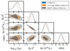 |
Fig. A.2. Bias due to different nonlinear modelling. The synthetic data are created by e-Mantis and fitted by two different models in the WL pessimistic case with baryons. |
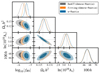 |
Fig. A.1. Bias due to different nonlinear modelling. The synthetic data are created by e-Mantis and fitted by two different models in the WL pessimistic case without baryons. |
Appendix B: Construction of the relative error
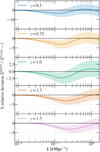 |
Fig. B.1. Relative difference between the power spectra from FORGE and ReACT. We show the relative deviation as the lines and the 68.3% confidence level as the shaded area. The boosts were all computed at the fiducial cosmology. |
To construct the relative error function, α(k, z), we can use the fact that Ξ(k, z) is constructed as the ratio to the same ΛCDM nonlinear power spectrum calculated with the halofit ‘Takahashi’ prescription in all models. This means that any deviations of the ΛCDM power spectrum from N-body simulations is also absorbed in Ξ. We can thus write the relative error as
 (B.1)
(B.1)
To construct ΔPδδ we follow the basic idea that all predictions for Ξ are equally accurate in calculating the modified gravity power spectrum. The true power spectrum is thus only known up to the spread of the predictions. To be conservative with our forecast, we choose to calculate the error from the difference between the FORGE predictions and the ReACT predictions, which is the largest among these predictions. This is shown in Fig. B.1. The ReACT prescription underpredicts the power spectrum at intermediate scales and overpredicts slightly at smaller scales. This is most likely due to ReACT handling the one- and two-halo power spectra separately. HMcode2020 predictions for the pseudo-cosmology nonlinear power spectrum also contribute to these inaccuracies as we can see by comparing the left and right panels of Figure 4 in Cataneo et al. (2019). To simplify the exact difference between these two codes, we argue that the theoretical error should plateau at the maximum deviation. This is because at nonlinear scales, the modes of different wave numbers are no longer independent of each other. By plateauing, we essentially say that we can no longer be more precise in the computation of the power spectrum on smaller scales.
Finally, we construct α using only the difference of the predictions at a fiducial of |fR0| = 5 × 10⁻⁶ in order not to bias our results. Our final fit has the form
 (B.2)
(B.2)
 (B.3)
(B.3)
![Mathematical equation: $$ \begin{aligned} k_{\rm p}(z)&= B_1 \, \exp \left[\mathrm{tanh} \left(\frac{z-B_2}{B_3}\right)\right]\,, \end{aligned} $$](/articles/aa/full_html/2025/06/aa52184-24/aa52184-24-eq81.gif) (B.4)
(B.4)
where we use x ≔ k/kp. We separately fit the amplitude function A(z) to the maximum deviation and the plateau wavenumber kp(z) to the wavenumber of maximum deviation. The best-fit values can be found in Table B.1 and are shown as the shaded region in Fig. B.1. We see that the zero line is within the 68.3% confidence bounds most of the time. This is in accordance with our construction that the two emulators should differ by the theoretical error.
Best-fit values of the relative error function.
All Tables
Fiducial values and flat prior ranges for cosmological parameters, |fR0| and IA parameters.
Mean, standard deviation, and 68.3% upper and lower limit of log10|fR0| for the WL optimistic setting
Mean, standard deviation, and 68.3% upper and lower limit of log10|fR0| for the WL pessimistic setting.
Mean, standard deviation, and 68.3% lower and upper limit of log10|fR0| for the optimistic setting.
Mean, standard deviation, and 68.3% lower and upper limit of log10|fR0| for the pessimistic setting.
Mean, standard deviation, and 68.3% lower and upper limit of log10|fR0| for the 3 × 2 pt pessimistic setting.
Mean, standard deviation, and 68.3% lower and upper limit of log10|fR0| for the 3 × 2 pt pessimistic setting
Mean, standard deviation, and 68.3% lower and upper limit of log10|fR0| for the WL optimistic setting with baryons.
Mean, standard deviation, and 68.3% lower and upper limit of log10|fR0| for the WL pessimistic setting with baryons.
Mean, standard deviation, and 68.3% lower and upper limit of log10|fR0| for the WL pessimistic setting.
Mean, standard deviation, and 68.3% lower and upper limit of log10|fR0| for the WL pessimistic setting with baryons.
All Figures
|
Fig. 1. Left panel: Comparisons between N-body simulations, e-Mantis and FORGE for |fR0| = 10−5. N-body data from simulations run by MG-AREPO and ECOSMOG codes are taken from the latest comparison project presented in Paper 1. We also include the prediction of FORGE where the cosmological parameters in the fiducial ΛCDM simulation, Ωm = 0.31315 and h = 0.6737, are used to make the prediction (FORGE Node 0). Right panel: Comparison of four prescriptions with an N-body simulation run by MG-AREPO. This simulation is one of the simulations used for training to construct the FORGE emulator (Node 13). The measurement of the power spectrum was done in Paper 2. |
| In the text | |
|
Fig. 2. Comparisons between all models considered for the HS6 fiducial cosmology for angular power spectra of WL (top left), galaxy clustering (top right) and their cross-correlation (bottom right) as well as for the matter power spectrum (bottom left). We show these for the WL redshift bin 6 and galaxy clustering bin 2, with the matter power spectrum plotted at z = 0.5, the redshift at which the kernels of both observables peak for the chosen bins. For all angular spectra, the error bands taken from the diagonal of the covariance are also shown. |
| In the text | |
|
Fig. 3. Constraints on parameters where the same model is used to create the synthetic data and perform the fitting such that the input parameters are reproduced. Left panel: WL optimistic case. Right panel: WL pessimistic case. |
| In the text | |
|
Fig. 4. Bias due to different nonlinear modelling. The synthetic data are created by FORGE and fitted by four different models. Left panel: WL optimistic case. Right panel: WL pessimistic case. |
| In the text | |
|
Fig. 5. Constraints from 3 × 2 pt analysis in the pessimistic setting. In the left panel, the same nonlinear model is used for the data and the fitting while in the right panel, the data are generated by FORGE. |
| In the text | |
|
Fig. 6. Effect of log10|fR0|, two baryonic parameters log10Mc and θej, and h on the WL angular power spectrum in bin 10. The dotted lines show predictions of e-Mantis with varying these parameters individually. The plot shows the ratio to the ΛCDM power spectrum. The plot includes the prediction of FORGE and e-Mantis with the fiducial parameters and the e-Mantis prediction using the best-fit values (log10|fR0| = −5.765, 100h = 65.736, log10(Mc) = 12.999) with the data created by FORGE. We can see that the e-Mantis prediction can fit the FORGE by adjusting these parameters. We note that the cosmological parameters for the ΛCDM power spectrum, |
| In the text | |
|
Fig. 7. Constraints on parameters from the WL optimistic setting with baryons. We show the case where e-Mantis is used to create both the data and fitting and the case where FORGE is used to create the data and it is fitted by e-Mantis. We also include the case where we impose a Gaussian prior on log10 Mc with the width of 0.2 in the case of FORGE fiducial data. Left panel: Constraints on baryonic parameters. Right panel: Constraints on cosmological parameters. |
| In the text | |
|
Fig. 8. Profile likelihood for log10|fR0| where FORGE is used to create data fitted by e-Mantis with baryons in the optimistic setting of WL. The square points show Δχ2 from the best-fit indicated by a diamond. The 95.5% confidence interval from the 1D marginalised posterior is shown as the error bar. The vertical dotted line indicates the input value of −log10|fR0| = 5.301. We see that the 1D marginalised posterior is shifted to smaller values of log10|fR0|. |
| In the text | |
|
Fig. 9. Constraints on parameters from the WL pessimistic setting with baryons. As in Fig. 7, we show the case where e-Mantis is used to create both the data and fitting as well as the case where FORGE is used to create the data and it is fitted by e-Mantis, ReACT and the fitting formula. Left panel: Constraints on baryonic parameters. Right panel: Constraints on cosmological parameters. |
| In the text | |
|
Fig. 10. Constraints on parameters from the WL pessimistic setting with baryons where the data are created in ΛCDM and it is fitted by e-Mantis. Left panel: Constraints on baryonic parameters. Right panel: Constraints on cosmological parameters. |
| In the text | |
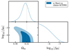 |
Fig. 11. Same as in Fig. 10, but we show the constraint on the derived quantity Ωm. |
| In the text | |
|
Fig. 12. Effect of adding theoretical errors. Left panel: Data are created by FORGE in the WL pessimistic setting and fitted by ReACT corrected by FORGE for fiducial cosmology, Eq. (41), with and without theoretical errors. Right panel: Data are created by e-Mantis in this case. |
| In the text | |
|
Fig. 13. Effect of adding theoretical errors in the presence of baryonic effects. Data are created by e-Mantis and fitted by ReACT corrected by FORGE for the fiducial cosmology with theoretical errors. For a comparison, we also show the result obtained by using e-Mantis to fit the same data. |
| In the text | |
|
Fig. A.2. Bias due to different nonlinear modelling. The synthetic data are created by e-Mantis and fitted by two different models in the WL pessimistic case with baryons. |
| In the text | |
|
Fig. A.1. Bias due to different nonlinear modelling. The synthetic data are created by e-Mantis and fitted by two different models in the WL pessimistic case without baryons. |
| In the text | |
|
Fig. B.1. Relative difference between the power spectra from FORGE and ReACT. We show the relative deviation as the lines and the 68.3% confidence level as the shaded area. The boosts were all computed at the fiducial cosmology. |
| In the text | |
Current usage metrics show cumulative count of Article Views (full-text article views including HTML views, PDF and ePub downloads, according to the available data) and Abstracts Views on Vision4Press platform.
Data correspond to usage on the plateform after 2015. The current usage metrics is available 48-96 hours after online publication and is updated daily on week days.
Initial download of the metrics may take a while.