| Issue |
A&A
Volume 693, January 2025
|
|
|---|---|---|
| Article Number | A249 | |
| Number of page(s) | 32 | |
| Section | Cosmology (including clusters of galaxies) | |
| DOI | https://doi.org/10.1051/0004-6361/202451611 | |
| Published online | 22 January 2025 | |
Euclid preparation
LVI. Sensitivity to non-standard particle dark matter models
1
Institute for Theoretical Particle Physics and Cosmology (TTK), RWTH Aachen University, 52056 Aachen, Germany
2
Department of Astrophysics, University of Zurich, Winterthurerstrasse 190, 8057 Zurich, Switzerland
3
Institute of Space Sciences (ICE, CSIC), Campus UAB, Carrer de Can Magrans, s/n, 08193 Barcelona, Spain
4
Dipartimento di Fisica, Università degli studi di Genova, and INFN-Sezione di Genova, Via Dodecaneso 33, 16146 Genova, Italy
5
SISSA, International School for Advanced Studies, Via Bonomea 265, 34136 Trieste, TS, Italy
6
Nordita, KTH Royal Institute of Technology and Stockholm 1859 University, Hannes Alfvéns väg 12, Stockholm SE-106 91, Sweden
7
Université Paris-Saclay, Université Paris Cité, CEA, CNRS, AIM, 91191 Gif-sur-Yvette, France
8
Dipartimento di Fisica “Aldo Pontremoli”, Università degli Studi di Milano, Via Celoria 16, 20133 Milano, Italy
9
INFN-Sezione di Milano, Via Celoria 16, 20133 Milano, Italy
10
Dipartimento di Fisica, Università degli Studi di Torino, Via P. Giuria 1, 10125 Torino, Italy
11
INFN-Sezione di Torino, Via P. Giuria 1, 10125 Torino, Italy
12
INAF-Osservatorio Astrofisico di Torino, Via Osservatorio 20, 10025 Pino Torinese (TO), Italy
13
Institut für Theoretische Physik, University of Heidelberg, Philosophenweg 16, 69120 Heidelberg, Germany
14
Institut de Recherche en Astrophysique et Planétologie (IRAP), Université de Toulouse, CNRS, UPS, CNES, 14 Av. Edouard Belin, 31400 Toulouse, France
15
Université St Joseph; Faculty of Sciences, Beirut, Lebanon
16
School of Mathematics and Physics, University of Surrey, Guildford, Surrey GU2 7XH, UK
17
INAF-Osservatorio Astronomico di Brera, Via Brera 28, 20122 Milano, Italy
18
INAF-Osservatorio di Astrofisica e Scienza dello Spazio di Bologna, Via Piero Gobetti 93/3, 40129 Bologna, Italy
19
Dipartimento di Fisica e Astronomia, Università di Bologna, Via Gobetti 93/2, 40129 Bologna, Italy
20
INFN-Sezione di Bologna, Viale Berti Pichat 6/2, 40127 Bologna, Italy
21
Max Planck Institute for Extraterrestrial Physics, Giessenbachstr. 1, 85748 Garching, Germany
22
Universitäts-Sternwarte München, Fakultät für Physik, Ludwig-Maximilians-Universität München, Scheinerstrasse 1, 81679 München, Germany
23
Dipartimento di Fisica, Università di Genova, Via Dodecaneso 33, 16146 Genova, Italy
24
INFN-Sezione di Genova, Via Dodecaneso 33, 16146 Genova, Italy
25
Department of Physics “E. Pancini”, University Federico II, Via Cinthia 6, 80126 Napoli, Italy
26
INAF-Osservatorio Astronomico di Capodimonte, Via Moiariello 16, 80131 Napoli, Italy
27
INFN section of Naples, Via Cinthia 6, 80126 Napoli, Italy
28
Instituto de Astrofísica e Ciências do Espaço, Universidade do Porto, CAUP, Rua das Estrelas, PT4150-762 Porto, Portugal
29
INAF-IASF Milano, Via Alfonso Corti 12, 20133 Milano, Italy
30
INAF-Osservatorio Astronomico di Roma, Via Frascati 33, 00078 Monteporzio Catone, Italy
31
INFN-Sezione di Roma, Piazzale Aldo Moro, 2 – c/o Dipartimento di Fisica, Edificio G. Marconi, 00185 Roma, Italy
32
Centro de Investigaciones Energéticas, Medioambientales y Tecnológicas (CIEMAT), Avenida Complutense 40, 28040 Madrid, Spain
33
Port d’Informació Científica, Campus UAB, C. Albareda s/n, 08193 Bellaterra, (Barcelona), Spain
34
Dipartimento di Fisica e Astronomia “Augusto Righi” – Alma Mater Studiorum Università di Bologna, Viale Berti Pichat 6/2, 40127 Bologna, Italy
35
Institute for Astronomy, University of Edinburgh, Royal Observatory, Blackford Hill, Edinburgh EH9 3HJ, UK
36
Jodrell Bank Centre for Astrophysics, Department of Physics and Astronomy, University of Manchester, Oxford Road, Manchester M13 9PL, UK
37
European Space Agency/ESRIN, Largo Galileo Galilei 1, 00044 Frascati, Roma, Italy
38
ESAC/ESA, Camino Bajo del Castillo, s/n., Urb. Villafranca del Castillo, 28692 Villanueva de la Cañada, Madrid, Spain
39
Université Claude Bernard Lyon 1, CNRS/IN2P3, IP2I Lyon, UMR 5822, Villeurbanne F-69100, France
40
Institute of Physics, Laboratory of Astrophysics, Ecole Polytechnique Fédérale de Lausanne (EPFL), Observatoire de Sauverny, 1290 Versoix, Switzerland
41
UCB Lyon 1, CNRS/IN2P3, IUF, IP2I Lyon, 4 rue Enrico Fermi, 69622 Villeurbanne, France
42
Departamento de Física, Faculdade de Ciências, Universidade de Lisboa, Edifício C8, Campo Grande, PT1749-016 Lisboa, Portugal
43
Instituto de Astrofísica e Ciências do Espaço, Faculdade de Ciências, Universidade de Lisboa, Campo Grande, 1749-016 Lisboa, Portugal
44
Department of Astronomy, University of Geneva, ch. d’Ecogia 16, 1290 Versoix, Switzerland
45
INAF-Istituto di Astrofisica e Planetologia Spaziali, Via del Fosso del Cavaliere, 100, 00100 Roma, Italy
46
Université Paris-Saclay, CNRS, Institut d’astrophysique spatiale, 91405 Orsay, France
47
INFN-Padova, Via Marzolo 8, 35131 Padova, Italy
48
Institut d’Estudis Espacials de Catalunya (IEEC), Edifici RDIT, Campus UPC, 08860 Castelldefels, Barcelona, Spain
49
Institut de Ciencies de l’Espai (IEEC-CSIC), Campus UAB, Carrer de Can Magrans, s/n Cerdanyola del Vallés, 08193 Barcelona, Spain
50
INAF-Osservatorio Astronomico di Trieste, Via G. B. Tiepolo 11, 34143 Trieste, Italy
51
Istituto Nazionale di Fisica Nucleare, Sezione di Bologna, Via Irnerio 46, 40126 Bologna, Italy
52
INAF-Osservatorio Astronomico di Padova, Via dell’Osservatorio 5, 35122 Padova, Italy
53
Institute of Theoretical Astrophysics, University of Oslo, PO Box 1029, Blindern, 0315 Oslo, Norway
54
Leiden Observatory, Leiden University, Einsteinweg 55, 2333 CC Leiden, The Netherlands
55
Jet Propulsion Laboratory, California Institute of Technology, 4800 Oak Grove Drive, Pasadena, CA 91109, USA
56
Department of Physics, Lancaster University, Lancaster LA1 4YB, UK
57
Felix Hormuth Engineering, Goethestr. 17, 69181 Leimen, Germany
58
Technical University of Denmark, Elektrovej 327, 2800 Kgs. Lyngby, Denmark
59
Cosmic Dawn Center (DAWN), Copenhagen, Denmark
60
Max-Planck-Institut für Astronomie, Königstuhl 17, 69117 Heidelberg, Germany
61
Department of Physics and Astronomy, University College London, Gower Street, London WC1E 6BT, UK
62
Department of Physics and Helsinki Institute of Physics, Gustaf Hällströmin katu 2, 00014 University of Helsinki, Finland
63
Aix-Marseille Université, CNRS/IN2P3, CPPM, Marseille, France
64
Université de Genève, Département de Physique Théorique and Centre for Astroparticle Physics, 24 quai Ernest-Ansermet, CH-1211 Genève 4, Switzerland
65
Department of Physics, PO Box 64, 00014 University of Helsinki, Finland
66
Helsinki Institute of Physics, Gustaf Hällströmin katu 2, University of Helsinki, Helsinki, Finland
67
European Space Agency/ESTEC, Keplerlaan 1, 2201 AZ Noordwijk, The Netherlands
68
NOVA optical infrared instrumentation group at ASTRON, Oude Hoogeveensedijk 4, 7991 PD Dwingeloo, The Netherlands
69
Universität Bonn, Argelander-Institut für Astronomie, Auf dem Hügel 71, 53121 Bonn, Germany
70
Aix-Marseille Université, CNRS, CNES, LAM, Marseille, France
71
Dipartimento di Fisica e Astronomia “Augusto Righi” – Alma Mater Studiorum Università di Bologna, Via Piero Gobetti 93/2, 40129 Bologna, Italy
72
Department of Physics, Centre for Extragalactic Astronomy, Durham University, South Road DH1 3LE, UK
73
Université Paris Cité, CNRS, Astroparticule et Cosmologie, 75013 Paris, France
74
Institut d’Astrophysique de Paris, 98bis Boulevard Arago, 75014 Paris, France
75
Institut d’Astrophysique de Paris, UMR 7095, CNRS, and Sorbonne Université, 98 bis boulevard Arago, 75014 Paris, France
76
IFPU, Institute for Fundamental Physics of the Universe, Via Beirut 2, 34151 Trieste, Italy
77
School of Mathematics, Statistics and Physics, Newcastle University, Herschel Building, Newcastle-upon-Tyne NE1 7RU, UK
78
Department of Physics, Institute for Computational Cosmology, Durham University, South Road DH1 3LE, UK
79
Institut de Física d’Altes Energies (IFAE), The Barcelona Institute of Science and Technology, Campus UAB, 08193 Bellaterra, (Barcelona), Spain
80
Department of Physics and Astronomy, University of Aarhus, Ny Munkegade 120, DK-8000 Aarhus C, Denmark
81
Waterloo Centre for Astrophysics, University of Waterloo, Waterloo, Ontario N2L 3G1, Canada
82
Department of Physics and Astronomy, University of Waterloo, Waterloo, Ontario N2L 3G1, Canada
83
Perimeter Institute for Theoretical Physics, Waterloo, Ontario N2L 2Y5, Canada
84
Space Science Data Center, Italian Space Agency, Via del Politecnico snc, 00133 Roma, Italy
85
Centre National d’Etudes Spatiales – Centre spatial de Toulouse, 18 avenue Edouard Belin, 31401 Toulouse Cedex 9, France
86
Institute of Space Science, Str. Atomistilor, nr. 409 Măgurele, Ilfov 077125, Romania
87
Instituto de Astrofísica de Canarias, Calle Vía Láctea s/n, 38204 San Cristóbal de La Laguna, Tenerife, Spain
88
Departamento de Astrofísica, Universidad de La Laguna, 38206 La Laguna, Tenerife, Spain
89
Dipartimento di Fisica e Astronomia “G. Galilei”, Università di Padova, Via Marzolo 8, 35131 Padova, Italy
90
Departamento de Física, FCFM, Universidad de Chile, Blanco Encalada 2008, Santiago, Chile
91
Universität Innsbruck, Institut für Astro- und Teilchenphysik, Technikerstr. 25/8, 6020 Innsbruck, Austria
92
Satlantis, University Science Park, Sede Bld 48940, Leioa-Bilbao, Spain
93
Instituto de Astrofísica e Ciências do Espaço, Faculdade de Ciências, Universidade de Lisboa, Tapada da Ajuda, 1349-018 Lisboa, Portugal
94
Universidad Politécnica de Cartagena, Departamento de Electrónica y Tecnología de Computadoras, Plaza del Hospital 1, 30202 Cartagena, Spain
95
INFN-Bologna, Via Irnerio 46, 40126 Bologna, Italy
96
Infrared Processing and Analysis Center, California Institute of Technology, Pasadena, CA 91125, USA
97
INAF, Istituto di Radioastronomia, Via Piero Gobetti 101, 40129 Bologna, Italy
98
Astronomical Observatory of the Autonomous Region of the Aosta Valley (OAVdA), Loc. Lignan 39, I-11020 Nus, (Aosta Valley), Italy
99
School of Physics and Astronomy, Cardiff University, The Parade, Cardiff CF24 3AA, UK
100
Center for Computational Astrophysics, Flatiron Institute, 162 5th Avenue, 10010 New York, NY, USA
101
Université Paris-Saclay, CNRS/IN2P3, IJCLab, 91405 Orsay, France
102
Centre de Calcul de l’IN2P3/CNRS, 21 avenue Pierre de Coubertin, 69627 Villeurbanne Cedex, France
103
Department of Mathematics and Physics E. De Giorgi, University of Salento, Via per Arnesano, CP-I93, 73100 Lecce, Italy
104
INAF-Sezione di Lecce, c/o Dipartimento Matematica e Fisica, Via per Arnesano, 73100 Lecce, Italy
105
INFN, Sezione di Lecce, Via per Arnesano, CP-193, 73100 Lecce, Italy
106
Junia, EPA department, 41 Bd Vauban, 59800 Lille, France
107
INFN, Sezione di Trieste, Via Valerio 2, 34127 Trieste, TS, Italy
108
ICSC – Centro Nazionale di Ricerca in High Performance Computing, Big Data e Quantum Computing, Via Magnanelli 2, Bologna, Italy
109
Instituto de Física Teórica UAM-CSIC, Campus de Cantoblanco, 28049 Madrid, Spain
110
CERCA/ISO, Department of Physics, Case Western Reserve University, 10900 Euclid Avenue, Cleveland, OH 44106, USA
111
Laboratoire Univers et Théorie, Observatoire de Paris, Université PSL, Université Paris Cité, CNRS, 92190 Meudon, France
112
Dipartimento di Fisica e Scienze della Terra, Università degli Studi di Ferrara, Via Giuseppe Saragat 1, 44122 Ferrara, Italy
113
Istituto Nazionale di Fisica Nucleare, Sezione di Ferrara, Via Giuseppe Saragat 1, 44122 Ferrara, Italy
114
Kavli Institute for the Physics and Mathematics of the Universe (WPI), University of Tokyo, Kashiwa, Chiba 277-8583, Japan
115
Ludwig-Maximilians-University, Schellingstrasse 4, 80799 Munich, Germany
116
Dipartimento di Fisica – Sezione di Astronomia, Università di Trieste, Via Tiepolo 11, 34131 Trieste, Italy
117
Minnesota Institute for Astrophysics, University of Minnesota, 116 Church St SE, Minneapolis, MN 55455, USA
118
Université Côte d’Azur, Observatoire de la Côte d’Azur, CNRS, Laboratoire Lagrange, Bd de l’Observatoire, CS 34229, 06304 Nice cedex 4, France
119
Institute for Astronomy, University of Hawaii, 2680 Woodlawn Drive, Honolulu, HI 96822, USA
120
Department of Physics & Astronomy, University of California Irvine, Irvine, CA 92697, USA
121
Department of Astronomy & Physics and Institute for Computational Astrophysics, Saint Mary’s University, 923 Robie Street, Halifax, Nova Scotia B3H 3C3, Canada
122
Departamento Física Aplicada, Universidad Politécnica de Cartagena, Campus Muralla del Mar, 30202 Cartagena, Murcia, Spain
123
Department of Physics, Oxford University, Keble Road, Oxford OX1 3RH, UK
124
Institute of Cosmology and Gravitation, University of Portsmouth, Portsmouth PO1 3FX, UK
125
Department of Computer Science, Aalto University, PO Box 15400, Espoo FI-00 076, Finland
126
Ruhr University Bochum, Faculty of Physics and Astronomy, Astronomical Institute (AIRUB), German Centre for Cosmological Lensing (GCCL), 44780 Bochum, Germany
127
DARK, Niels Bohr Institute, University of Copenhagen, Jagtvej 155, 2200 Copenhagen, Denmark
128
Univ. Grenoble Alpes, CNRS, Grenoble INP, LPSC-IN2P3, 53, Avenue des Martyrs, 38000 Grenoble, France
129
Department of Physics and Astronomy, Vesilinnantie 5, 20014 University of Turku, Finland
130
Serco for European Space Agency (ESA), Camino bajo del Castillo, s/n, Urbanizacion Villafranca del Castillo, Villanueva de la Cañada, 28692 Madrid, Spain
131
ARC Centre of Excellence for Dark Matter Particle Physics, Melbourne, Australia
132
Centre for Astrophysics & Supercomputing, Swinburne University of Technology, Hawthorn, Victoria 3122, Australia
133
School of Physics and Astronomy, Queen Mary University of London, Mile End Road, London E1 4NS, UK
134
Department of Physics and Astronomy, University of the Western Cape, Bellville, Cape Town 7535, South Africa
135
ICTP South American Institute for Fundamental Research, Instituto de Física Teórica, Universidade Estadual Paulista, São Paulo, Brazil
136
Oskar Klein Centre for Cosmoparticle Physics, Department of Physics, Stockholm University, Stockholm SE-106 91, Sweden
137
Astrophysics Group, Blackett Laboratory, Imperial College London, London SW7 2AZ, UK
138
INAF-Osservatorio Astrofisico di Arcetri, Largo E. Fermi 5, 50125 Firenze, Italy
139
Dipartimento di Fisica, Sapienza Università di Roma, Piazzale Aldo Moro 2, 00185 Roma, Italy
140
Centro de Astrofísica da Universidade do Porto, Rua das Estrelas, 4150-762 Porto, Portugal
141
Dipartimento di Fisica, Università di Roma Tor Vergata, Via della Ricerca Scientifica 1, Roma, Italy
142
INFN, Sezione di Roma 2, Via della Ricerca Scientifica 1, Roma, Italy
143
Institute of Astronomy, University of Cambridge, Madingley Road, Cambridge CB3 0HA, UK
144
Theoretical astrophysics, Department of Physics and Astronomy, Uppsala University, Box 515, 751 20 Uppsala, Sweden
145
Department of Physics, Royal Holloway, University of London, London TW20 0EX, UK
146
Mullard Space Science Laboratory, University College London, Holmbury St Mary, Dorking, Surrey RH5 6NT, UK
147
Department of Astrophysical Sciences, Peyton Hall, Princeton University, Princeton, NJ 08544, USA
148
Niels Bohr Institute, University of Copenhagen, Jagtvej 128, 2200 Copenhagen, Denmark
149
Center for Cosmology and Particle Physics, Department of Physics, New York University, New York, NY 10003, USA
⋆ Corresponding author; julien.lesgourgues@physik.rwth-aachen.de
Received:
22
July
2024
Accepted:
18
October
2024
The Euclid mission of the European Space Agency will provide weak gravitational lensing and galaxy clustering surveys that can be used to constrain the standard cosmological model and its extensions, with an opportunity to test the properties of dark matter beyond the minimal cold dark matter paradigm. We present forecasts from the combination of the Euclid weak lensing and photometric galaxy clustering data on the parameters describing four interesting and representative non-minimal dark matter models: a mixture of cold and warm dark matter relics; unstable dark matter decaying either into massless or massive relics; and dark matter undergoing feeble interactions with relativistic relics. We modelled these scenarios at the level of the non-linear matter power spectrum using emulators trained on dedicated N-body simulations. We used a mock Euclid likelihood and Monte Carlo Markov chains to fit mock data and infer error bars on dark matter parameters marginalised over other parameters. We find that the Euclid photometric probe (alone or in combination with cosmic microwave background data from the Planck satellite) will be sensitive to the effect of each of the four dark matter models considered here. The improvement will be particularly spectacular for decaying and interacting dark matter models. With Euclid, the bounds on some dark matter parameters can improve by up to two orders of magnitude compared to current limits. We discuss the dependence of predicted uncertainties on different assumptions: the inclusion of photometric galaxy clustering data, the minimum angular scale taken into account, and modelling of baryonic feedback effects. We conclude that the Euclid mission will be able to measure quantities related to the dark sector of particle physics with unprecedented sensitivity. This will provide important information for model building in high-energy physics. Any hint of a deviation from the minimal cold dark matter paradigm would have profound implications for cosmology and particle physics.
Key words: cosmological parameters / cosmology: observations / dark matter / large-scale structure of Universe
© The Authors 2025
 Open Access article, published by EDP Sciences, under the terms of the Creative Commons Attribution License (https://creativecommons.org/licenses/by/4.0), which permits unrestricted use, distribution, and reproduction in any medium, provided the original work is properly cited.
This article is published in open access under the Subscribe to Open model. Subscribe to A&A to support open access publication.
1. Introduction
Understanding the nature of dark matter (DM) is one of the priority targets within the communities of cosmology, astroparticle physics, and high-energy physics. Over the past decade, the Large Hadron Collider (LHC) results and the absence of direct or indirect DM detection have shown that the situation concerning the nature of DM is wide open. Weakly interacting massive particles (WIMPs) are only one candidate among many possibilities (Bertone et al. 2005; Feng 2010). Particle-like DM could have a large range of plausible masses, lifetimes, annihilation cross-sections, and scattering cross-sections.
The standard cosmological model makes the working assumption of a purely stable, decoupled, and cold dark matter (CDM) species, which can be modelled as dust in simulations of the evolution of the Universe since very early times – well before photon decoupling. In the CDM limit, the only measurable parameter related to DM is its relic non-relativistic density today, ρcdm, which can be expressed in terms of a dimensionless density parameter, ωcdm := Ωcdmh2, where Ωcdm is the fractional density of CDM (relative to the critical density) and h := H0/(100 kms−1 Mpc−1) is the reduced Hubble parameter. However, in non-minimal scenarios, DM could have several other parameters of possible relevance for fitting cosmological observations, such as: a non-negligible velocity dispersion (Bond & Szalay 1983; Bode et al. 2001), a lifetime not considerably larger than the age of the Universe (e.g. Ichiki et al. 2004; Audren et al. 2014), and cross-sections describing either its self-interaction (Spergel & Steinhardt 2000; Feng et al. 2009) or its feeble interaction with other species (Boehm et al. 2001; Cyr-Racine et al. 2016).
From the point of view of a particle physics model-builder, non-minimal DM models are easy to motivate; typically, they do not require more complicated or more fine-tuned ingredients that the particle physics models leading to plain CDM. The logic pursued successfully by high-energy physicists for almost a century consists of postulating additional symmetries (rather than adding individual particles) in order to explain unaccounted experimental results. The current standard model of particle physics is known to be incomplete (Workman et al. 2022) and the assumption of new symmetries usually comes together with a rich dark sector; that is, several new particles with new interactions, with potentially more than one population surviving until today and
contributing to DM or dark radiation. From this point of view, having just one decoupled, stable, and cold relic in our Universe does not sound much more natural than being surrounded by one or more dark species with potentially non-trivial properties. High-energy physicists often suggest that, given the richness of the visible sector, there is no obvious reason for the dark sector to reduce to a single CDM relic particle.
The astrophysics community is sometimes reluctant to investigate the possible consequences of non-minimal particle-physics assumptions in cosmology as long as the minimal ΛCDM model has not been ruled out. The situation is, however, evolving given the accumulation of tensions or unresolved questions in cosmological observations (like the small-scale CDM crisis, Hubble tension, or S8 tension; see for instance Verde et al. 2019, Abdalla et al. 2022). In this context, it sounds at least reasonable to investigate the possibility of detecting some effects induced by non-minimal DM models. Of course, it is still possible that future observations only provide bounds on these models and leave us with plain CDM as a preferred case. Even in this case, it would be extremely interesting for particle physics model-builders to have such bounds, since constraints from accelerators or astroparticle experiments usually probe a different regime or different model assumptions than cosmological data.
Non-minimal DM properties may affect the growth of structures in the Universe in different ways, at different times, and on different scales. Thus, they can leave several types of signatures in the two-point correlation function of matter fluctuations in Fourier space, called the matter power spectrum. This spectrum can be reconstructed from several types of cosmological observations at different redshifts. The modified growth of structure induced by non-minimal DM models could also affect other statistical probes of structure formation (higher-order correlation functions, halo mass function, peak and void statistics), but in this work we only consider its impact on the matter power spectrum.
Euclid (Euclid Collaboration: Mellier et al. 2025) is a medium-class mission of the European Space Agency, which will map the local Universe to improve our understanding of the expansion history and of the growth of structures. The satellite will observe roughly 15 000 deg2 of the sky through two instruments, a visible imager (VIS, Euclid Collaboration: Cropper et al 2025) and a Near-Infrared Spectrometer and Photometer (NISP, Euclid Collaboration: Jahnke et al. 2025), delivering the images of more than one billion galaxies and the spectra of tens of millions of galaxies out to redshift of about 2. The combination of spectroscopy and photometry will allow us to reconstruct the matter power spectrum up to an accuracy of 1%.
Since the matter power spectrum could be strongly affected by the nature of DM, Euclid is a perfect tool for testing non-minimal DM properties. It may either confirm the standard CDM paradigm or discover some new DM features. The goal of this work is precisely to estimate the sensitivity of Euclid to different DM parameters beyond its mere relic density. Given the wide range of possible alternatives to standard CDM, we cannot explore all possibilities. We instead concentrate on four examples of non-minimal scenarios that are still compatible with current data and that could be either constrained or detected by Euclid. Our choice of models is dictated by simple considerations. First, we should select some representative cases. Since in non-minimal models, DM particles are expected to either free-stream (with some velocity dispersion) and/or decay (with some rate) and/or scatter (with some cross-sections), we go through examples in each of these three categories. A well-motivated example of DM with a velocity dispersion is warm DM. Some simple examples of decaying DM consist of particles with a constant decay rate, decaying into either relativistic or non-relativistic daughter particles; and a representative case of scattering DM is that of DM interacting with dark radiation. Second, we are interested in models such that galaxy redshift surveys could provide stronger bounds than other observables, and in particular, than cosmic microwave background (CMB) and/or Lyman-α forest data. For reasons detailed in the next sections, this would not be the case for pure warm DM or pure decaying DM. Thus, going to the next level of complexity, we assume a mixture of either cold and warm DM, or of stable and unstable particles. In conclusion, we focus on four interesting and representative models: a mixture of cold and warm DM, a mixture of stable and unstable particles decaying into either relativistic or non-relativistic particles, and DM interacting with dark relativistic relics.
Euclid will deliver several types of observations. Among these, the weak lensing (WL) survey and the galaxy clustering (GC) photometric survey will be ideal to constrain DM properties, since they will both provide a measurement of the matter power spectrum down to small scales and up to high redshift. These two surveys will return maps in tomographic bins that can be analysed all together (taking into account cross-correlations between WL and galaxy density maps). In addition to this joint data set, called the photometric probe, Euclid will provide other observations. The Euclid spectroscopic galaxy redshift survey will play an essential role in constraining several cosmological models and parameters. Cluster number counts will also convey very useful information. However, these surveys will not provide information on such small scales as WL, and their implementation in sensitivity forecasts relies on a different methodology than for the photometric probe. In particular, they require a different approach to model non-linear effects for each non-minimal DM model. Thus, for simplicity, we choose to concentrate only on the Euclid photometric probe in this work.
In Sect. 2 of this work, we review the four DM models that we investigate, with a brief discussion of their foundations, their free parameters, and their effects on the linear matter power spectrum. In Sect. 3, we explain how to model the effect of these scenarios at the level of the non-linear power spectrum, using emulators trained on dedicated N-body simulations. In Sect. 4, we summarise the assumptions and numerical pipelines used in our parameter sensitivity forecasts for the Euclid photometric probe. We present our results for each model in Sect. 5 and provide final conclusions in Sect. 7.
2. Non-minimal particle dark matter models
Many particle DM properties can be tested with cosmology (Gluscevic et al. 2019). As was mentioned in the introduction, we only focus here on four particular models. On the one hand, these models constitute representative samples of the three most plausible properties of non-minimal particle DM: a non-negligible velocity dispersion, some decay rate, or a non-negligible scattering rate. On the other hand, within their respective category, they account for the simplest scenarios that can be constrained better by WL and galaxy surveys than CMB and Lyman-α data.
2.1. Cold plus warm dark matter
In this model, a fraction, fwdm, of the total DM fractional density, Ωdm, is assumed to be warm, so that Ωdm = Ωcdm + Ωwdm = (1 − fwdm) Ωdm + fwdm Ωdm. The warm dark matter (WDM) component possesses a thermal (root mean square) velocity vrms that depends on the temperature-to-mass ratio Twdm/mwdm. WDM would revert to CDM in the limit vrms → 0, or equivalently mwdm → ∞.
This mixed cold plus warm dark matter (CWDM) model has been studied previously, for instance, in Boyarsky et al. (2009a), Schneider (2015), Murgia et al. (2017), Murgia et al. (2018), Parimbelli et al. (2021), or Hooper et al. (2022). It may account either for cosmologies with two distinct DM components, or also, effectively, for cosmologies with a single DM component with a non-thermal distribution, such as resonantly produced sterile neutrinos (Boyarsky et al. 2009b). This model has been often invoked as a possible solution to the small-scale CDM crisis (Anderhalden et al. 2013; Maccio et al. 2013). Current best constraints come from Lyman-α forest surveys (Hooper et al. 2022), Milky Way satellites (Diamanti et al. 2017), and WL surveys (Hervas-Peters et al. 2024; see Sect. 5.1).
The thermal velocity of WDM defines its maximum free-streaming scale, reached at the time of its non-relativistic transition during radiation domination. On larger wavelengths, cosmological fluctuations have the same evolution as in a model in which all the DM would be cold. On smaller scales, the perturbations of the WDM component are negligible and the growth of CDM density fluctuations is suppressed. Thus, at the level of linear perturbations, the overall effect of WDM is to induce a step-like suppression in the matter power spectrum. The amplitude of the step is controlled by fwdm1. The shape of the step is universal for all models in which the WDM phase-space distribution has a thermal shape up to a rescaling factor. This covers two well-known limits: on the one hand, thermal WDM, for which the phase-space distribution is thermal (with no rescaling factor) but the WDM temperature, Twdm, is reduced compared to the active neutrino temperature, due to its earlier decoupling time; and the Dodelson–Widrow (DW) model (Dodelson & Widrow 1994; Colombi et al. 1996), for which the phase-space distribution is identical to that of active neutrinos (with Twdm = Tν) up to a rescaling factor χ ≪ 1 accounting for the efficiency of active-sterile neutrino oscillations in the early Universe with a small mixing angle, χ ∼ sin2θ. For this broad category of models, the location of the step-like suppression is controlled by the thermal velocity; that is, by the temperature-to-mass ratio, Twdm/mwdm.
It is convenient to parameterise the location of the step in terms of the rescaled mass
where Tν is the current value of the active neutrino temperature computed in the instantaneous decoupling limit; that is, such that Tν/Tγ = (4/11)1/3. For the class of models described above, the effect of WDM is entirely described by the two parameters (fwdm, x), independently of the chosen model (thermal WDM or DW). In the DW case, x coincides with  . In the thermal case, one has
where we used the fact that for Fermi–Dirac thermal relics X with a temperature TX = Tν one gets mX = 94.1 ΩXh2 eV2.
In this model, the evolution of linear cosmological perturbation can be computed with the public version of CLASS. Then, to account for the thermal WDM case, we pass to the code the parameters Ωwdmh2 = fwdm Ωdmh2,  , and finally
  with x inferred from Eq. (2)3. In principle one could use a different set of parameters for the equivalent DW model and find the exact same linear power spectra (Lesgourgues 2011; Blas et al. 2011; Lesgourgues & Tram 2011). Figure 1 shows the power spectrum at redshift zero for several CWDM models rescaled by that of a pure ΛCDM model, for various values of (fwdm, x) but fixed values of the usual ΛCDM parameters (Ωm, Ωb, h, As, ns) accounting respectively for the fractional density of total non-relativistic matter (baryonic plus dark), the fractional density of baryonic matter, the reduced Hubble parameter, and the amplitude and spectral index of the primordial spectrum of scalar (curvature) perturbations. In the left panel, we vary x (or equivalently
  ) with fixed fwdm to check that x only controls the location of the step. In the right panel we do the opposite to show that fwdm controls its amplitude.
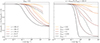 |
Fig. 1. Ratio of the linear (solid lines) and non-linear (dashed lines) power spectra of several CWDM models to that of a pure ΛCDM model with the same cosmological parameters, parameterised by the fraction fwdm and the rescaled mass x. The other parameters (Ωdm, Ωb, h, As, ns) are kept fixed. All spectra are computed today (z = 0). These plots cover all the cases in which WDM has a Fermi–Dirac distribution possibly rescaled by a factor χ, including the limits of the thermal WDM (χ = 1) and Dodelson–Widrow (Twdm = Tν) models. In the latter case x coincides with the physical mass. The non-linear spectra are predicted by the emulator introduced in Sect. 3.1 and plotted up to the maximum wavenumber at which this emulator is trusted. |
In Sect. 3.1, we show how to compute the impact of CWDM on the non-linear matter spectrum. In Sect. 5.1, we perform Euclid forecasts on the parameter of the CWDM model. For that purpose, we use a Bayesian MCMC approach to fit the CWDM model to mock Euclid data, assuming a logarithmic prior on fwdm ∈ [2 × 10⁻³, 1] and a flat prior on ![$ m_{\mathrm{wdm}}^{\mathrm{thermal}} \in [10 \, \mathrm{eV},\,1\,\mathrm{keV}] $](/articles/aa/full_html/2025/01/aa51611-24/aa51611-24-eq7.gif) .
.
Such a logarithmic prior on fwdm allows us to assess precisely the constraining power of Euclid even when fwdm is very small (e.g. in the range from 10−3 to 10−1). This limit is the most interesting in the case of the Euclid probes since, in this case, the data may be compatible with a relatively small WDM mass, and thus a small step located on relatively large wavelengths, in the range probed by WL and GC surveys in the linear and mildly non-linear regime. Large values of fwdm (e.g. in the range from 0.1 to 1) imply a strong suppression of the power spectrum that is already excluded by Lyman-α forest data unless the mass is really large – a limit in which, from the point of view of Euclid data, CWDM would be indistinguishable from pure CDM.
2.2. Dark matter with one-body decay
If DM particles are unstable, they may decay in different ways into lighter particles. Cosmological observables are not sensitive to all details concerning the nature of the decay products, but they depend on simple considerations like the fact that these decay products could be relativistic or non-relativistic. In the simplest scenario, all decay products are assumed to be ultra-relativistic and can be considered as a single species, dubbed dark radiation (DR). This simple model of decaying dark matter (DDM) is often called one-body decaying DM and abbreviated as 1b-DDM.
In this section, we assume that DM is made up of two cold species: a fraction 1 − fddm of stable dark matter (CDM) and a fraction fddm of 1b-DDM decaying into DR. For simplicity, we assume a constant decay rate, Γddm = 1/τddm, where τddm is the lifetime of the decaying species. The current value of the fractional dark radiation density, Ωdr, is not an independent parameter of the model: it can be computed consistently for each value of fddm and Γddm.
This model has been studied previously; for instance, in Ichiki et al. (2004), Audren et al. (2014), Berezhiani et al. (2015), Chudaykin et al. (2016), Chudaykin et al. (2018), Oldengott et al. (2016), Poulin et al. (2016), Pandey et al. (2020), Xiao et al. (2020), Nygaard et al. (2021), Schöneberg et al. (2022), Simon et al. (2022), Holm et al. (2023), or Bucko et al. (2023). It has been often invoked as a possible solution to the Hubble and/or S8 tension. The best constraints at the moment come from CMB plus baryon acoustic oscillation (BAO) data (Nygaard et al. 2021), galaxy surveys (Simon et al. 2022), and WL surveys (Bucko et al. 2023; see Sect. 5.2).
In this model, the evolution of linear cosmological perturbations can be computed with the public version of CLASS4. The code accepts two possible definitions of the decaying DM fraction: one can either pass the value of fddm today, taking the effect of decay into account, or the value  evaluated at some initial time τini ≪ τddm, before any significant decay has occurred,
Here we choose to report results on  , for the purpose of easier comparison with previously published bounds. Some related parameters are
  (respectively
  ), the fractional density that DDM (respectively total DM) would have today if DDM did not decay. The free parameters of the 1b-DDM model are then (Γddm,
  ,
,  , Ωb, h, As, ns), while the cosmological constant parameter ΩΛ is adjusted to match the budget equation in a flat universe5.
If one varies the two decaying DM parameters (Γddm,  ) while fixing the other parameters (
 , Ωb, h, As, ns), one changes the predicted age of the Universe, which controls the amplitude of the matter power spectrum on all scales, as well as the redshift of radiation-to-matter equality, which determines the scale of the overall peak in the spectrum. These effects cause an enhancement of the matter power spectrum on scales larger than those crossing the Hubble radius around the time of equality, corresponding to comoving wavenumbers k < 2–3 × 10⁻³ h Mpc−1, and a suppression on smaller scales. For wavenumbers k ≥ 10−1 h Mpc−1, the power spectrum is suppressed by a constant factor with respect to the ΛCDM case. A larger fraction,
  , or a higher rate, Γddm, both imply a smaller amplitude of the power spectrum on these scales. Actually, the suppression factor is found to depend essentially on the product
  , as is illustrated in Fig. 2. In the left panel, we vary
  while keeping the product
  fixed to 0.005 Gyr−1 (a value representative of the constraints found in the result Sect. 5.2). Then, the power spectrum of the 1b-DDM model is found to be independent of
  up to the order of one per mille. Thus, we anticipate that the parameter
  alone is difficult to constrain with Euclid data. Instead, in the right panel of Fig. 2, we vary the product
  while keeping
  fixed. We clearly see a change in the suppression factor for k ≥ 10−1 h Mpc−1 and in the slope of the power spectrum for k ∼ 10−2 h Mpc−1, potentially detectable using Euclid probes.
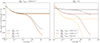 |
Fig. 2. Ratio of the linear (solid lines) and non-linear (dashed lines) power spectra of several 1b-DDM models to that of a pure ΛCDM model with the same cosmological parameters, parameterised by the fraction |


In Sect. 3.2, we compute the impact of the 1b-DDM model on the non-linear matter spectrum. In Sect. 5.2, we fit the 1b-DDM model to mock Euclid data. In order to obtain fast-converging MCMC chains, we adopt some flat priors on  and
and  , with prior edges detailed in Sect. 5.2, but we expect interesting constraints only on the second parameter.
2.3. Dark matter with two-body decay
In the next-to-simplest cosmological model of DDM, a cold DDM particle with a large mass, mddm, and a constant decay rate, Γddm, is assumed to decay into a first massless daughter particle and a second massive daughter particle with mass mdaughter. This model is dubbed two-body decaying DM (2b-DDM). The parent particle is assumed to account for a fraction,  , of the initial CDM budget, defined in the same way as for one-body decay (see Eq. (3)), with the remaining fraction
  corresponding to ordinary stable CDM. In each decay, the fraction of energy transferred from the parent particle to the first massless daughter particle, ε, can be related to the mass ratio:
In the limit mdaughter → mddm, all the energy goes into the second massive daughter, but since this corresponds to the conversion of one CDM particle into another one, the model is indistinguishable from the standard ΛCDM model. In the opposite limit mdaughter → 0, the two daughter particles are ultra-relativistic and share the same amount of energy, which corresponds to ε = 0.5: this limit is equivalent to the 1-body decay model introduced in the previous section. However, in the more interesting range 0 < ε < 0.5, the second daughter particle can behave as WDM. Aoyama et al. (2014) have shown that for the purpose of computing cosmological observables one only needs to specify the three parameters (fddm, Γddm, ε) on top of the usual ΛCDM parameters.
This model has been studied previously, for instance, in Aoyama et al. (2014), Vattis et al. (2019), Haridasu & Viel (2020), Franco Abellán et al. (2022, 2021), Schöneberg et al. (2022), Simon et al. (2022), or Bucko et al. (2024). It has also been invoked as a possible solution to the H0 and/or S8 tension. The best constraints at the moment come from CMB plus BAO data (Schöneberg et al. 2022), galaxy surveys (Simon et al. 2022), and WL surveys (Bucko et al. 2024; see Sect. 5.3). Finally, Franco Abellán et al. (2024) have shown how to perform efficient sensitivity forecasts based on machine learning techniques for this model.
At the level of linear perturbation theory, this model is implemented in a branch of CLASS developed and publicly released6 by the authors of Franco Abellán et al. (2021, 2022). Figure 3 shows the effect on the linear power spectrum of a variation in the parameters (Γddm, ε,  ) for fixed ΛCDM parameters. We see that this model leads to a step-like suppression of the matter power spectrum, which is not surprising since, in this case, DM is split between a CDM and a WDM component. The shape of the step is, however, different from the CWDM case, because the warm component gets produced progressively and affects different scales at different times. Figure 3 focuses on cases with ε ≪ 0.5 for which, in each decay, most of the energy is transferred from one non-relativistic DM species to another one. Thus, while the universe expands, the energy density of total matter evolves almost like in the case of stable DM, ρm ∝ a−3, and the age of the universe is not significantly affected by the DDM parameters. This explains why in Fig. 3 we do not see any effect of the 2b-DDM parameters on the matter power spectrum on very large scales (k ≪ 10−1 h Mpc−1), as it was the case for 1b-DDM. As a side note, one can observe tiny oscillations in the linear power spectrum ratios of Figure 3. This is most likely a numerical artefact caused by the use of a fluid approximation for the perturbations of the warm species within a fixed range of scales. The same figure shows that these spurious oscillations are smoothed out by the emulator introduced in Sect. 3.3. Thus, they cannot affect our results7.
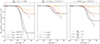 |
Fig. 3. Ratio of the linear (solid lines) and non-linear (dashed lines) power spectra of several two-body DDM models to that of a pure ΛCDM model with the same cosmological parameters, parameterised by the fraction |


The parameter ε controls the velocity of the daughter particle just after the decay, which reads  in the centre of mass frame (the subscript k refers to ‘kick’, since the daughter particles get a velocity kick). Thus, by analogy with WDM, ε determines the free-streaming scale and the location of the step in the power spectrum. The parameters (Γddm,
  ) both control the abundance of 2b-DDM as a function of time and thus the linear growth rate of the total DM density fluctuation δdm(a). Hence these parameters both control the amplitude of the step. The ΛCDM limit is recovered for ε = 0 and/or
  and/or Γddm = 0.
In Sect. 3.3, we show how to compute the impact of the 2b-DDM model on the non-linear matter spectrum. In Sect. 5.3, we fit the 2b-DDM model to mock Euclid data. We perform our sensitivity forecast with flat priors on  , with prior edges detailed in that section.
2.4. ETHOS n = 0
The ETHOS framework (Cyr-Racine et al. 2016) is a general attempt to parameterise physically plausible interactions in a dark sector featuring at least one type of non-relativistic relics (playing the role of cold interacting dark matter, IDM) and one type of ultra-relativistic relics (playing the role of interacting dark radiation, IDR). The theory provides a mapping between phenomenological parameters describing the relevant interaction rates and fundamental parameters appearing in the Lagrangian of the dark sector. In particular, the ETHOS index n describes to the power-law dependence of the IDR-IDM interaction rate Γidr − idm on the temperature of the dark sector.
The case n = 0 is of particular interest, because it corresponds to an IDM-IDR momentum exchange rate Γidm − idr scaling like the Hubble radius during radiation domination (Buen-Abad et al. 2015; Cyr-Racine et al. 2016; Becker et al. 2021). Thus, in this model, the ratio Γidm − idr/H (where both Γidm − idr and H depend on time) remains constant during radiation domination and decreases slowly during matter domination. This means that IDM and IDR can remain in a regime of feeble but steady interactions until equality. The IDR-IDM interactions then become gradually irrelevant at the beginning of matter domination and negligible during the formation of non-linear structures. On the other hand, ETHOS models with n > 0 tend to suppress the power spectrum very sharply below some scale. Thus, similar to pure WDM models, they are easier to constrain with Lyman-α data than with galaxy surveys.
This model can be motivated with some concrete and plausible particle physics set up, such as non-Abelian DM (Buen-Abad et al. 2015). It is interesting from the point of view of cosmology phenomenology because it introduces a very smooth suppression in the matter power spectrum (Lesgourgues et al. 2016; Buen-Abad et al. 2018) – instead of oscillatory patterns or an exponential cut-off as would be the case for ETHOS models with n > 0. The power spectrum suppression shape is also very different from the one caused by a hot or warm DM component. This model is often invoked as a solution to the S8 tension (Lesgourgues et al. 2016; Buen-Abad et al. 2018) – or even to the Hubble tension, but this is no longer the case with recent data (Schöneberg et al. 2022). Current constraints on this model are obtained with CMB data combined with Lyman-α data (Archidiacono et al. 2019; Hooper et al. 2022) or with the full-shape power spectrum of the BOSS galaxy redshift survey (Rubira et al. 2023; see Sect. 5.4).
This model can be parameterised in terms of the IDR-IDM scattering amplitude, Γidr − idm(z*), at some arbitrary reference redshift z*, of the density of DM (through Ωidmh2), and of the density of DR (through Ωidrh2). Following the rest of the literature, we choose a reference redshift z* = 107 and express the effective comoving rate of IDR scattering off IDM as

Assuming IDR with a thermal spectrum and two fermionic degrees of freedom, we can parameterise the IDR density in terms of the IDR-to-photon temperature ratio, Tidr/Tγ = ξidr ≤ 1, such that  . The contribution of IDR to the effective number of neutrinos is then given by ΔNeff = (Tidr/Tν)4 with Tν defined in the instantaneous neutrino decoupling limit; that is, ΔNeff = (11/4)4/3ξidr4 ≃ 3.85 ξidr4. The ratio ξidr is a dimensionless parameter. Γidr − idm is a rate and adark is an inverse distance that we express in Mpc−1 (this definition and choice of units has no other purpose than matching the conventions of the CLASS code and of previous work studying this model)8. Finally, in the ETHOS framework, one needs to specify the self-interaction rate between IDR particles. The non-Abelian DM model and the CMB+Lyman-α constraints of Lesgourgues et al. (2016), Buen-Abad et al. (2018), Archidiacono et al. (2019), or Hooper et al. (2022) assumed a strongly self-interacting IDR fluid. One may assume instead free-streaming IDR, and Rubira et al. (2023) consider the two cases. These two different assumptions are expected to have a small impact on CMB constraints (due to the effect of IDR fluctuations dragging the photons fluctuations before decoupling) but a negligible impact on constraints from large-scale structure (because IDR self-interactions are irrelevant for the growth rate of IDM). Here we stick to the assumption of free-streaming IDR.
The most important physical effect of this model on the matter power spectrum comes from the fact that the IDR-IDM interactions tend to slow down the growth rate of DM fluctuations on sub-Hubble scales during radiation domination, and to suppress the power spectrum on small scales at all subsequent times (Lesgourgues et al. 2016; Buen-Abad et al. 2015). Actually, as is mentioned in Archidiacono et al. (2019), the power spectrum suppression is mainly sensitive to the effective comoving scattering rate of IDR off IDM, which is given by
Since ρidr is proportional to ξidr4 while ρidm is normalised by the measurement of Ωidmh2, this rate is controlled mainly by the parameter combination adark ξidr4. Therefore, we expect the amplitude of the suppression in the linear matter power spectrum to depend strongly on adark ξidr4 and weakly on the orthogonal combination, except in the case of sufficiently large ξidr4, in which the effect of additional radiation with a given ΔNeff also comes into play. Indeed, an enhancement of ΔNeff has some well-known effects on the matter and CMB power spectra, explained for instance in Lesgourgues & Verde (2022), and we expect Euclid to be sensitive to this effect (Euclid Collaboration: Archidiacono et al. 2025).
The ETHOS formalism is implemented in the public version of CLASS9. We show in Fig. 4 the effect of varying the parameters ξidr or adark ξidr4 with fixed values of all other cosmological parameters.
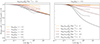 |
Fig. 4. Ratio of the linear (solid lines) and non-linear (dashed lines) power spectra of several free-streaming ETHOS n = 0 models to that of a pure ΛCDM model with the same cosmological parameters, parameterised by the dark-radiation-to-photon temperature ratio ξidr and interaction strength adark. The effects are displayed in the basis (ξidr, adark ξidr4) to show that the combination adark ξidr4, which gives the scattering rate of IDR off IDM, controls the amplitude of the small-scale suppression of the linear matter power spectrum. The other parameters ( |

In the left panel, the scattering rate controlled by adark ξidr4 is fixed, which explains the constant suppression of the linear power spectrum in the large-k limit. When log10(ξidr) varies from −1.2 to −0.6, ΔNeff increases from 6.1 × 10⁻⁶ to 0.015, which is too small to directly affect the matter power spectrum. However, these different values of ξidr and thus adark have an impact on intermediate scales: they control the maximum scale at which IDM feels the interaction, and thus the wavenumber at which the matter power spectrum starts to be suppressed. When log10(ξidr) reaches −0.4, the radiation density gets enhanced by a non-negligible amount, ΔNeff = 0.097. This results in an additional suppression of the linear power spectrum on small scales.
In the right panel, the amount of IDR is fixed to a small value but the effective scattering rate is increased, leading to more and more suppression. This suppression has a different shape to the case of WDM: it behaves like a transition to a smaller spectral index rather than an exponential cut-off.
In Sect. 3.4, we show how to compute the impact of the ETHOS n = 0 model on the non-linear matter spectrum. In Sect. 5.4, we fit this model to mock Euclid data. We perform our sensitivity forecast with flat priors on {log10(adarkξidr4/Mpc−1), log10ξidr}, with prior edges detailed in that section.
3. Emulating the non-linear evolution
To predict observable WL and galaxy correlation spectra, one needs to know the non-linear matter power spectrum for each model. Since N-body simulations are computationally too expensive for being run at each point in MCMC chains, it is customary to use a restricted set of N-body simulations to build emulators of the non-linear matter power spectrum. These emulators should be accurate compared to the sensitivity of the experiment within the range of model parameters covered by our priors, and fast to evaluate within MCMC runs. In this section, we describe the emulators used in our MCMC forecasts for each of the four non-minimal DM models described in Sect. 2.
Instead of directly emulating the non-linear power spectrum of the extended cosmological model,  , it is customary to emulate the ratio
and to compute the final observable spectra using

This strategy offers two main advantages. Firstly, it is easier to generate accurate training data for the ratio 𝒮model(k,z) than for the final spectrum, since several N-body simulation artefacts tend to cancel out in the ratio (e.g. resolution effects at small scale, or residual noise from cosmic variance and mesh assignment on large scale). Secondly, the final spectrum depends on all cosmological and DM parameters, but the ratio 𝒮model(k,z) does not in some cases. This ratio depends on course on the DM parameters, but not necessarily on each single parameter of the ΛCDM model. In each model, one can perform some explicit tests to investigate this dependence and build the emulator on a reduced parameter space.
In this work, we need to decide which tool we should use for predicting the first factor in Eq. (8); that is, the spectrum  . In principle, we could use fitting functions like Halofit (Smith et al. 2003) or HMcode 2020 (Mead et al. 2021), emulators like the EuclidEmulator2 (Knabenhans et al. 2021) or BACCOemulator (Angulo et al. 2021), etc. In the future, when analysing real data, we shall use the best tool available at that time in order to get unbiased results. But for the purpose of the present work, which is to forecast the sensitivity to DM parameters, one could use essentially any of these tools without changing the results on the DM parameter sensitivity, provided that the same tool is used when generating fiducial data and when fitting theoretical predictions. Our choice shall be specified in the next sections.
In the context of this work, having accurate predictions for the ratio 𝒮model(k,z) is more important. With a noisy emulator, one could get slightly wrong predictions for the effect of DM parameters on the final observable spectra, and potentially underestimate degeneracies between these parameters and cosmological or baryonic feedback parameters. In the forecasts presented here, we use emulators designed to achieve per-cent level accuracy up to k ∼ 𝒪(10) h Mpc−1 and z ∼ 2.5 (in the next section we provide further details on the accuracy of each emulator). Given the sensitivity of Euclid, this is sufficient for robust forecasts. There are some plans to keep training these emulators and improving their accuracy in order to be sure that, when analysing real data, the error coming from the emulator is clearly subdominant in the total systematic error budget.
3.1. Cold plus warm dark matter
To predict the non-linear suppression in the matter power spectrum in CWDM scenarios, we use an improved version of the emulator already described in Parimbelli et al. (2021). Such an emulator is trained on a large set of N-body simulations, covering a large parameter space, for a total of 100 models with different WDM fractions fwdm and WDM masses. The simulations explicitly assume thermal WDM, but this assumption is not relevant in the final analysis: as long as one performs the mass conversion described in Sect. 2.1 before calling the emulator, the latter still applies to all models in which WDM has a Fermi–Dirac distribution possibly rescaled by a factor χ. The simulations cover masses down to  , but we have checked that the emulator provides a consistent extrapolation down to
  for small fractions
  (see Hervas-Peters et al. 2024). For each model, four realisations are run with fixed amplitudes: two with different random phases and two with the opposite phases. The box size is set to 120 h−1 Mpc in order to reconnect with the linear regime at large scales for all redshifts and without any significant discontinuity and to obtain percent-level convergence up to k ≈ 10 h Mpc−1. The (fixed) cosmological parameters are Ωm = 0.315, Ωb = 0.049, h = 0.674, ns = 0.965, and a value of As that would give σ8 = 0.811 in the pure ΛCDM limit (where σ8 is the square root of the variance of matter fluctuations in spheres of radius 8 h−1 Mpc).
Initial conditions are set at z = 99 with a modified version of the N-GenIC code (Springel et al. 2005), using a linear power spectrum obtained from CLASS (Blas et al. 2011). The simulations are run with the tree-particle mesh (TreePM) code GADGET-III (Springel et al. 2005) and follow the gravitational evolution of 5123 particles. Snapshots are taken starting from z = 3.5 down to z = 0, linearly spaced with Δz = 0.5. Once the power spectra from these snapshots are measured, we take their ratio with respect to the corresponding ΛCDM spectrum and build the emulator following the exact same procedure as in Parimbelli et al. (2021). This new tool emulates the first 20 principal components of the power spectrum suppression using Gaussian processes. It is trained on the redshift range z ∈ [0 − 3.5] and in the range of scales k ∈ [0.07 − 25] h Mpc−1. The performances are found to be comparable to the ones stated in Parimbelli et al. (2021); that is, the difference between the emulated and the simulated suppressions never exceeds ∼1.5%. All in all, the non-linear matter power spectrum in the presence of CWDM is given by

where the last term is precisely what the emulator predicts and  is computed with the version of Halofit revisited by Takahashi et al. (2012) and Bird et al. (2012).
We plot a few examples of predictions for the non-linear spectrum at z = 0 (compared to the linear predictions of CLASS) in Fig. 1. We can clearly see that the suppression of power induced by the WDM component on small scales is much smaller in the non-linear (rather than linear) power spectrum. This is a well-known effect of mode-mode coupling when perturbations become non-linear. The smaller is the redshift, the less pronounced is the power spectrum suppression on scales smaller than the maximum free-streaming scale.
A few considerations about the simulations must be made here. For the sake of computational efficiency, all the particles in all the realisations are initialised as cold particles, even in the runs containing WDM. This assumption has a twofold implication. First, we assume that the differences between a CWDM model and ΛCDM reside in the initial conditions and in their linear power spectra; second, we are neglecting WDM thermal velocities. We tested the impact of these two assumptions by running a further realisation, with fwdm = 0.2 and  , in which we initialise 5123 CDM particles as well as 5123 more particles as Type2, with the correct thermal velocities10. This value of fwdm has been chosen because, below this fraction, current data are compatible with any value for mwdm; the value of the mass has been chosen in order to have a ∼50% suppression in the linear power spectrum at k ∼ 5 h Mpc−1. We show the results of this test in Fig. 5. In the left plot, we compare the matter power spectrum suppression at various redshifts when neglecting thermal velocities (solid orange lines) and when fully considering them (dashed violet lines). As can be noted, differences between the two treatments are only relevant at z ≳ 2 and for k ≳ 5 h Mpc−1. The right plot shows instead the ratios between the angular power spectra of cosmic shear (or equivalently WL, orange), the cross-correlation between GC and galaxy lensing (red), and GC (purple), computed according to the prescriptions described in Sect. 4, using each of the two sets of power spectra in the left plot. We use a single bin here for simplicity, ranging from z = 0 to z = 3.5, and neglect intrinsic alignment. Differences are well below percent level; for comparison, at ℓ = 104, the Euclid sample variance is expected to be ∼1.6%. We can conclude that our assumptions do not introduce any systematic effects in the analysis.
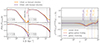 |
Fig. 5. Left: Effect of neglecting the WDM thermal velocities in CWDM simulations with fwdm = 0.2 and |

3.2. Dark matter with one-body decay
We employed the fitting functions found by Hubert et al. (2021) to model the non-linear matter power spectrum in the presence of one-body decay. These fits are inspired by fitting functions published in Enqvist et al. (2015) and built upon N-body simulations implementing DDM into the PKDGRAV3 code (Potter et al. 2017).
We have seen in Sect. 2.2 that 1b-DDM induces a suppression in the linear matter power spectrum that is asymptotically constant on intermediate and small scales, with a suppression factor proportional to  , or to
  . The amplitude and redshift dependence of this suppression factor is given by
where α, β, γ are functions of ωb := Ωbh2, h, and ωm := Ωbh2 + Ωdmh2. We refer to Hubert et al. (2021) and Bucko et al. (2023) for their detailed form. We note that the suppression functions εlin(z) and εnonlin(k, z) introduced respectively in Eqs. (10, 11) should not be confused with the parameter ε of the 2b-DDM model. The non-linear evolution imprints an additional suppression that can be inferred from N-body simulations. Enqvist et al. (2015) provided a fit to the non-linear suppression function εnonlin(k, z) in the case  that Hubert et al. (2021) generalised to arbitrary values of the DDM fraction. The suppression function is estimated from N-body simulations for a fixed cosmology. Since only late-time DM decays are of interest, the initial conditions of such N-body simulations are identical to those in a ΛCDM scenario. However, to account for the 1b-DDM, the particle masses are being gradually decreased in the simulation as a function of the rate Γddm, the fraction
  and the simulation time, mimicking the decay process (for more details, see Hubert et al. 2021). The suite of N-body simulations used to construct the fitting functions was run with a box size of 500 h−1 Mpc evolving 10243 particles. The cosmological parameters were fixed to fiducial values Ωm = 0.307, Ωb = 0.048, 109As = 2.43, h = 0.678, and ns = 0.96. The convergence of the 1b-DDM N-body simulations was studied in Hubert et al. (2021) with the conclusion that the implementation of the model is trustworthy at least up to k ≃ 6.4 h Mpc−1. Finally, Hubert et al. (2021) argue that εnonlin(k, z) is nearly cosmology-independent and can be extrapolated to cosmologies well beyond those probed in our work.
The fitting function provides the suppression of the matter power spectrum with respect to the fiducial ΛCDM cosmology, P1b − DDM(k, z)/PΛCDM(k, z) = 1 − εnonlin(k, z), with
The suppression function interpolates from the linear behaviour on intermediate scales, εnonlin(k, z)→εlin(z), to a power-law suppression on small scales with εnonlin(k, z)∝kp1 − p2. The factors a1, a2, p1, and p2 are given for each lifetime τddm and redshift z by
These fitting functions are publicly available as a part of the DMemu package,11 and designed to reproduce the results of N-body simulations with a precision better than 1% up to k = 13 h Mpc−1. We note that, at a given redshift, the fitting functions of Eq. (12) depend only on τddm (or Γddm), while εlin depends only on  . Thus, the non-linear evolution lifts the degeneracy between Γddm and
  observed at the level of the linear power spectrum.
In order to match the linear predictions of CLASS on large and intermediate scales with those of the fitting functions on intermediate and small scales without introducing any discontinuity, we use the following ansatz to calculate the non-linear matter power spectrum of the 1b-DDM model:
with the non-linear ΛCDM spectrum evaluated with the version of Halofit revisited by Takahashi et al. (2020) and Bird et al. (2012). Then, firstly, on intermediate (linear) scales, the second and third factor in the right-hand side of Eq. (13) go to one, and one recovers P1b − DDM(k, z)→P1b − DDM, lin(k, z). Secondly, on smaller (non-linear) scales, after noticing that we can rewrite Eq. (13) as
![$$ \begin{aligned} P_{\rm 1b-DDM}(k,z)&= \frac{P_{\rm 1b-DDM, lin}(k,z)}{1-\varepsilon _{\rm lin}(z)} \, \frac{P_{\Lambda \mathrm{CDM}}(k,z)}{P_{\Lambda \mathrm{CDM,lin}}(k,z)} \nonumber \\&\times [1-\varepsilon _{\rm nonlin}(k,z)] \, , \end{aligned} $$](/articles/aa/full_html/2025/01/aa51611-24/aa51611-24-eq65.gif)
and that the first fraction tends towards PΛCDM,lin(k,z), we get
![$$ \begin{aligned} P_{\rm 1b-DDM}(k,z) \longrightarrow P_{\rm \Lambda \mathrm {CDM}}(k,z) \, [1-\varepsilon _{\rm nonlin}(k,z)] \, , \end{aligned} $$](/articles/aa/full_html/2025/01/aa51611-24/aa51611-24-eq66.gif)
that is, the approximation to the non-linear 1b-DDM power spectrum provided by the emulator. Equation (13) is designed to provide a smooth transition between these two limits. According to this ansatz, the ratio P1b − DDM(k, z)/PΛCDM(k, z) is given by the boost factor
We already saw in Fig. 2 the ratio of 1b-DDM-to-ΛCDM linear power spectra, as well as the ratio of non-linear spectra given by Eq. (16). Figure 6 is similar to Fig. 2 but shows additionally the raw result of the emulator; that is, the ratio P1b − DDM(k, z)/PΛCDM(k, z)≃1 − εnonlin(k, z) above k ≳ 0.05 h Mpc−1 (dashed lines). The linear prediction (solid lines) and the raw emulator (dashed lines) match each other quite well around k = 0.05 h Mpc−1, but switching abruptly from one to the other at a given wavenumber would introduce a small discontinuity in the spectrum. Dotted lines show the boost factor defined in Eq. (16) and used in our pipeline. This factor provides a very smooth interpolation from the prediction of CLASS to that of the emulator.
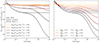 |
Fig. 6. Effect of 1b-DDM parameters on the linear (solid) and non-linear (dashed) matter power spectrum. Left: Effect of varying the decay rate Γddm with a fixed fraction |


3.3. Dark matter with two-body decay
To model the two-body decays up to non-linear scales, we use the emulator published in Bucko et al. (2024), which can provide the 2b-DDM-to-ΛCDM non-linear power spectrum ratio
up to z ≃ 2.3 and k ≃ 6 h Mpc−1. The emulator was trained on approximately 100 PKDGRAV3N-body simulations directly implementing the late-time DM decays, while starting from ΛCDM-like initial conditions at zini = 49. Bucko et al. (2024) set Lbox = 125, 250, 512 h−1 Mpc and N = 2563, 5123, 10243 depending of each specific DDM configuration, in such way to achieve converged simulations up to kmax = 6h Mpc−1. Bucko et al. (2024) argue that the suppression 𝒮2b(k, z) is approximately independent of cosmology and fix the standard cosmological parameters to Ωm = 0.307, Ωb = 0.048, 109As = 2.43, h = 0.678, and ns = 0.96 in the simulations. At each simulation time step, a number of DM particles is randomly selected for decay. The decay into a lighter daughter particle is accounted for through a velocity kick with amplitude vk and random direction. In the limit ε ≪ 0.5 considered here, vk is approximately given by c ε. These kicks lead to suppression in the matter power spectrum below the free-streaming length of the massive daughter particles controlled by vk ∼ c ε.
The emulator predicts 𝒮2b(k, z) using a combination of a ‘Principal Component Analysis’ (PCA) with feed-forward ‘sinusoidal representation networks’ (SIRENs; see Sitzmann et al. (2020)). Within the emulation process, the PCA is used to compress the power spectrum ratios 𝒮2b(k, z), taking into account 5 principal components. Then, the SIREN architecture is trained in a supervised fashion to predict these principal components given the input parameters of 2b-DDM model and the redshift of interest. The loss function of the network is the square distance of the input and output 2b-DDM-to-ΛCDM ratio, reconstructed from the PCA components predicted by the network. The emulator covers the case of an arbitrary fraction ![$ f_{\mathrm{ddm}}^{\mathrm{ini}} \in [0,\,1] $](/articles/aa/full_html/2025/01/aa51611-24/aa51611-24-eq72.gif) of long-lived DDM particles with
of long-lived DDM particles with  decaying into non-relativistic daughters with vk ≲ 5000 km s−1, corresponding to ε < 0.017. The emulator can predict ratios of 2b-DDM and ΛCDM nonlinear matter power spectra up to z = 2.3 and k ≃ 6 h Mpc−1, with a precision better than 1% at the 68% CL. It is implemented inside the publicly available DMemu package introduced after Eq. (12). We already compared the emulator result to the linear 2b-DDM-to-ΛCDM linear power spectrum ratio in Fig. 3.
Like in other cases, the final non-linear power spectrum of the 2b-DDM model is obtained by mutiplying the non-linear power spectrum of the ΛCDM model (computed using Halofit) with the emulated ratio 𝒮2b(k, z).
3.4. ETHOS n = 0
The non-linear matter power spectrum of the ETHOS n = 0 model is predicted by a dedicated emulator that will be presented in Bucko et al. (in prep.). Like for the 1b-DDM and 2b-DDM cases, this emulator will be released within the DMemu package. It assumes the particular case in which IDR consists of two free-streaming fermionic degrees of freedom. It predicts the ETHOS-to-ΛCDM non-linear power spectrum ratio
up to z = 3 and k ≃ 5 h Mpc−1. The architecture used to train the ETHOS emulator is similar to the one used in the 2b-DDM scenario, described in Sect. 3.3, with slight modifications. First of all, only 4 PCA components are used to compress the input ETHOS-to-ΛCDM matter power spectra, while the SIREN architecture involves two dense hidden layers with 256 neurons each. The emulator provides below 1% errors at the aforementioned scales and redshifts, within the range of ETHOS models defined by the N-body simulations discussed in the next paragraphs.
The emulator is built upon a suite of N-body simulations which have been run using PKDGRAV3 with Lbox = 325 h−1 Mpc and N = 5123, assuming a fiducial cosmology with ωidm := Ωidmh2 = 0.1202, ωb = 0.02236, h = 0.6727, ns = 0.9649, and 109As = 2.101. One massive neutrinos species with mν = 0.06 eV was included. Instead of using a typical back-scaling approach to generate the initial conditions, Bucko et al. (in prep.) follow an alternative method described in Tram et al. (2019). The “true” initial conditions are generated using the C0NCEPT code (Dakin et al. 2022). In combination with CLASS, C0NCEPT also computes the linear evolution of all species (photons, metric, neutrinos, IDR, IDM). This information is used to calculate the gravitational potential at each time step in the PKDGRAV3 simulation. In this way, the DM particles of the simulation feel their own gravity, taken into account at the non-linear level, plus the gravity from other species, modelled at the linear level.
The simulations used to train the emulator implement the ETHOS n = 0 only through modified initial conditions at zini = 49. The effect of IDM-IDR scattering at z < zini is neglected. This assumption is valid only for model parameters such that the scattering rate Γidm − idr is negligible compared to the Hubble rate at z = zini. Since the rate Γidm − idr is computed with respect to conformal time, it should be compared to the conformal Hubble rate ℋ = aH. Rubira et al. (2023) provide an analytical approximation for the (redshift-dependent) interaction rate to Hubble rate ratio,
![$$ \begin{aligned} \frac{\Gamma _{\rm idm-idr}}{\mathcal{H} }&\simeq 0.0152\left( \frac{a_{\rm dark}}{1000\, \mathrm{Mpc^{-1}}} \right)\left(\frac{\xi _{\rm idr}}{0.1} \right)^4 \nonumber \\&\times \frac{(1+z)^2}{\left[\Omega _{\mathrm{m}}(1+z)^3 + \Omega _{{\gamma }}(1+z)^4(1+\xi ^4_{\rm idr}) + \Omega _\Lambda \right]^{1/2}}\, . \end{aligned} $$](/articles/aa/full_html/2025/01/aa51611-24/aa51611-24-eq75.gif)
Assuming Ωm = 0.27 and ξidr4 ≪ 1, this gives approximately Γidm − idr/ℋ ≃ adarkξidr4/(0.48 Mpc−1) at z = 49. Bucko et al. (in prep.) suggest to trust the simulations and the emulator as long as this ratio is smaller than 0.1. In first approximation, this is the case for adarkξidr4 < 0.05 Mpc−1. We shall see in Sect. 5.4 that this region is appropriate to study the sensitivity of Euclid to ETHOS parameters, at least when the fiducial model is assumed to be ΛCDM (or close to it).
We plot the magnitude of the ratio given by Eq. (19) at z = 49 as a function of (ξidr, adark) in the left panel of Fig. 7. The region where the emulator is to be trusted lays below the solid black line. Dashed lines in the left panel of Fig. 7 correspond to models with either log10(adark/Mpc−1) = 1.0 (dashed) or ξidr = 0.25 (dash-dotted), for which we show the emulator predictions in the right panel of the same figure. Namely, the dashed curves show the power spectrum suppression as a function of ξidr, ranging from the ΛCDM limit for ξidr = 0.0 up to ξidr = 0.4, while fixing log10(adark/Mpc−1) to 1.0. Similarly, the dash-dotted lines show the emulator output for ξidr = 0.25 varying the coupling strength adark from 10−3 Mpc−1 to 109.5 Mpc−1. We note that some of the cases shown in the right panel stand outside of the region Γidm − idr/ℋ ≤ 0.1 in which the emulator is to be fully trusted.
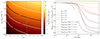 |
Fig. 7. Left: Ratio of the interaction rate between IDM and IDR (Γidm − dr) and comoving Hubble rate (ℋ) as a function of the dark-radiation-to-photon temperature ratio ξidr and interaction strength adark, computed at the redshift zini = 49 at which the N-body simulations used to construct the ETHOS emulator are initialised. We display the contours of equal ratio as solid white lines and highlight the threshold value of 0.1 in black. We further depict the region with adark = 10 Mpc−1 (dashed grey) and ξidr = 0.25 (dash-dotted grey). Right: Power spectrum suppression 𝒮ETHOS(k, z) predicted by the emulator for parameters chosen along each of the two grey lines of the left panel. |
The effect of the ETHOS parameters on the non-linear power spectrum is also shown in Fig. 4 in the (ξidr, adarkξidr4) basis. While at the linear level the suppression of the matter power spectrum is mainly controlled by the combination adarkξidr4, we see that at the non-linear level ξidr also plays a significant role for fixed adarkξidr4.
3.5. Baryonic feedback
Baryonic feedback processes can alter the gas distribution around DM halos, causing a deviation between the total matter distribution and the distribution of DM (e.g. Chisari et al. 2018; van Daalen et al. 2020). These processes induce a suppression of the total matter power spectrum Pm on small scales that may be somewhat similar to the effect of non-minimal DM and induce degeneracies between baryonic and DM parameters (see e.g. Hubert et al. 2021). Hence, for our purposes, it is crucial to incorporate these processes into our modelling framework. In this study, we use the BCemu framework12 (Giri & Schneider 2023) to address this concern. The BCemu framework serves as an emulator for the suppression 𝒮bf(k) caused by baryonic feedback. Consequently, the total non-linear matter power spectrum in a given cosmological model, Pm, can be expressed as

where Pm, no bf(k, z) is the total matter power spectrum neglecting baryonic feedback effects at redshift z.
BCemu has been used in several recent WL studies (e.g. Schneider et al. 2022; Grandis et al. 2024). It is based on the baryonic correction modelling framework of Schneider & Teyssier (2015), Schneider et al. (2019), and Giri & Schneider (2021). This framework parameterises the stellar and gas profiles at a given redshift with seven baryonic parameters. Giri & Schneider (2021) analysed these baryonic parameters and found that three parameters are enough to model the suppression seen in hydrodynamical simulations at scales k ≲ 10 h Mpc−1 and at a given redshift. We use this three-parameter model in this work.
Two of these parameters describe the gas profile in halos of given virial radius, rvir, and virial mass, Mvir, modelled as
![$$ \begin{aligned} \rho _{\rm gas}(r)\propto \frac{\Omega _{\rm b}/\Omega _{\rm m} -f_{\rm star}(M_{\rm vir})}{\left[1+10\frac{r}{r_{\rm vir}}\right]^{\beta (M_{\rm vir})}\left[1+\frac{r}{\theta _{\rm ej}r_{\rm vir}}\right]^{\frac{2}{5}[7-\beta (M_{\rm vir})]}} \, , \end{aligned} $$](/articles/aa/full_html/2025/01/aa51611-24/aa51611-24-eq77.gif)
with a total stellar fraction, fstar(Mvir), and a mass-dependent index,
The former function is assumed to be known,
Thus, in this model, the gas profile only depends on two free parameters: a critical mass M′c such that small halos with Mvir ≪ Mc have a gas profile shallower than the Navarro–Frenk–White profile, and an ejection factor θej giving the ratio of the gas ejection radius to the virial radius. The BCemu model also involves assumptions concerning the stellar profile of the central galaxy. The fraction of stars in the central galaxy, fcga(Mvir), is given by a relation similar to fstar(Mvir), but with a different exponent,
where the index ηδ is an additional free parameter.
In summary, the minimal BCemu model relies on three free parameters (M′c, θej, ηδ) impacting, respectively, the overall suppression induced by baryonic feedback, the maximum scales affected by the suppression, and the upturn of 𝒮bf(k,z) at large k. In order to deal only with dimensionless parameters, Schneider et al. (2022) redefine the first one as Mc := M′c/(1 h−1 M⊙). Figure 2 in Schneider et al. (2019) shows the impact of these parameters on the matter power spectrum. In the BCemu model, the only cosmology dependence of 𝒮bf(k,z) comes through the baryon fraction Ωb/Ωm.
In particular, we assume no explicit dependence of the baryonic feedback suppression function 𝒮bf(k,z) on the parameters describing non-standard DM models. This assumption was shown to be valid at least for k < 5 h Mpc−1 in the CWDM scenario (see Sect. 3.4 in Parimbelli et al. 2021). This conclusion is expected to apply also to the other DM scenarios studied here in which, like in the CWDM case, DM particles are decoupled at low redshift and behave either as CDM or WDM. In our analysis, smaller scales with k > 5 h Mpc−1 only have a small contribution to the spectra  involving the first two WL redshift bins. Thus, the findings of Parimbelli et al. (2021) suggest that we can safely neglect the impact of non-standard DM on baryonic feedback. More generally, we can think of the effect of non-standard DM and of BF on the non-linear matter power spectrum as two leading-order effects, of a few percent each within the range of scales relevant in our analysis, and that of non-standard DM on BF as a next-to-leading order effect of a few percent squared; that is, a few per mille. It is thus reasonable to neglect this correction in a first analysis.
We refer interested readers to Giri & Schneider (2021) for a more detailed description of the BCemu parameters.
The redshift evolution of 𝒮bf(k,z) is modelled by making each of the three baryonic parameters b redshift dependent as

where νb is a free parameter. This leads to a total of six parameters to model the baryonic feedback. In our choice of fiducial values and priors, we restrict the values of νb such that the baryonic parameters {log10Mc, θej, ηδ} remain within the range of the parameter space where BCemu is trained.
While it is known that the WL signal is modified at small scales by baryonic feedback effects, the situation is much less clear regarding the GC signal. Since galaxies act as tracers of the underlying DM distribution, they are not directly affected by the ejection of gas via feedback processes. We rather expect an indirect effect caused by the relaxation of the DM potential reacting to the ejection of gas. Since we do not know the true amplitude of this indirect effect, we consider two extreme cases where the GC is either unchanged by baryonic feedback or it is affected in the same way as the WL. We expect the truth to lie somewhere between these two cases.
4. Forecast methodology
4.1. Likelihood
We use a standard formalism to describe the Euclid photometric likelihood already presented, for instance, in Audren et al. (2013b), Euclid Collaboration: Blanchard et al. (2020), Euclid Collaboration: Archidiacono et al. (2025), Casas et al. (2024). The galaxy images of the WL survey and the galaxy positions of the GC photometric survey are binned into N redshift bins. In each bin, the raw data can be processed into two-dimensional spherical maps of either the lensing potential field density in the WL case or the galaxy density field in the GCph case. The maps are decomposed into spherical harmonics with coefficients ai(ℓ, m) for each redshift bin i. Each ai is assumed to obey a Gaussian distribution with covariance matrix ![$ C_{ij}(\ell) = \frac{1}{2\ell+1}\sum_ma_i(\ell,m)[a_i(\ell,m)]^* $](/articles/aa/full_html/2025/01/aa51611-24/aa51611-24-eq83.gif) . The Cij(ℓ) are the observed power spectra of WL or GCph in harmonic space and can be compared to theoretical predictions.
. The Cij(ℓ) are the observed power spectra of WL or GCph in harmonic space and can be compared to theoretical predictions.
In our forecasts, we assume that the power spectra observed by Euclid coincides with the theoretical predictions of a given fiducial cosmology with spectra  arising from multipoles aifid such that
 ![$ C_{ij}^{\mathrm{fid}}(\ell) = \frac{1}{2\ell+1}\sum_m a_i^{\mathrm{fid}}(\ell,m)[a_i^{\mathrm{fid}}(\ell,m)]^* $](/articles/aa/full_html/2025/01/aa51611-24/aa51611-24-eq85.gif) . The likelihood ℒ of the observed data given a theoretical model with spectrum
. The likelihood ℒ of the observed data given a theoretical model with spectrum  is then given by
![$$ \begin{aligned} \mathcal{L}&= \mathcal{N} \prod _{\ell ,m} \left[ \det \mathsf{C}^\mathrm{th}(\ell )\right]^{-1/2} \nonumber \\&\times \exp \left\{ -f_{\rm sky}\frac{1}{2}\sum _{ij}a_i^\mathrm{fid}(\ell ,m) \,\, (C_{ij}^\mathrm{th})^{-1}(\ell ) \,\, [a_j^\mathrm{fid}(\ell ,m)]^*\right\} \, , \end{aligned} $$](/articles/aa/full_html/2025/01/aa51611-24/aa51611-24-eq87.gif)
where 𝒩 is a normalisation factor, and partial sky coverage is approximately accounted for through multiplication with the sky fraction fsky. This can be rewritten as (Audren et al. 2013b)
![$$ \begin{aligned} \chi ^2&:= -2\ln \frac{{\mathcal{L} }}{{\mathcal{L} }_{\rm max}} \nonumber \\&= f_{\rm sky}\sum _\ell (2\ell +1)\left\{ \mathrm{Tr}[(\mathsf{C}^\mathrm{th})^{-1}(\ell )\,\,\mathsf{C}^\mathrm{fid}(\ell )] \right. \nonumber \\&~~~~~~~~~~~~~~~~~~~~~~~~~~~+ \left. \ln \frac{\det \mathsf C ^\mathrm{th}(\ell )}{\det \mathsf C ^\mathrm{fid}(\ell )} -N\right\} \nonumber \\&= f_{\rm sky}\sum _\ell (2\ell +1)\left\{ \frac{d_\ell ^\mathrm{mix}}{d_\ell ^\mathrm{th}}+\ln \frac{d_\ell ^\mathrm{th}}{d_\ell ^\mathrm{fid}}-N\right\} \, , \end{aligned} $$](/articles/aa/full_html/2025/01/aa51611-24/aa51611-24-eq88.gif)
where N is the size of the matrices Cth(ℓ) and Cfid(ℓ), while
for each of the theoretical and fiducial spectra. Finally, the mixed determinant is defined as
![$$ \begin{aligned} d_\ell ^\mathrm{mix} := \sum _{k = 1}^N \det \left[ {\left\{ \begin{array}{ll} C_{ij}^\mathrm{th}(\ell )&\mathrm{for}\;j\ne k \\ C_{ij}^\mathrm{fid}(\ell )&\mathrm{for}\;j=k \end{array}\right.} \right]\, , \end{aligned} $$](/articles/aa/full_html/2025/01/aa51611-24/aa51611-24-eq90.gif)
such that in each term of the sum, the determinant is evaluated over a matrix in which the k-th column of the theory matrix Cth has been substituted by the k-th column of the fiducial matrix Cfid.
We then perform MCMC forecasts (Audren et al. 2013b; Casas et al. 2024) using this likelihood. The likelihood is incorporated into the MontePython package13 (Audren et al. 2013a; Brinckmann & Lesgourgues 2019) for Bayesian parameter inference. The role of MontePython is to fit the fiducial spectra under the assumption of a given theoretical model with a set of free parameters. A few independent Monte Carlo Markov Chains sample the likelihood by exploring the parameter space according to the Metropolis-Hastings algorithm, until some convergence criterium is reached. The best-fit model coincides by construction with the fiducial model, while the marginalised credible interval of each parameter provide an estimate of the sensitivity of Euclid to this parameter.
4.2. Observable power spectra
The model for the spectra  used in the likelihood, where X = L (respectively X = G) refers to the WL (respectively GC) probe and i = 1, …, Ni to the bin number, is detailed in Euclid Collaboration: Blanchard et al. (2020), Euclid Collaboration: Archidiacono et al. (2025), Casas et al. (2024). The final expression is given by
where WiX(k, z) are the window functions of the X probe, H(z) is the Hubble rate at redshift z, r(z) the comoving distance to an object at redshift z, Pm(k, z) the matter power spectrum evaluated at wavenumber k, and  the noise spectrum. The boundaries zmin and zmax, defined in Table 1, specify the redshift range covered by the survey. The relation k(ℓ, z) is inferred from the Limber approximation (Kaiser 1992; Kilbinger et al. 2017),
Specifications used in our mock Euclid photometric likelihood in the pessimistic (pess.) and optimistic (opt.) cases.
which is sufficiently accurate for ℓ > ℓmin, where ℓmin is given in Table 1 (see however Tanidis & Camera 2019). Assuming a Poissonian distribution of galaxies, the noise spectra read
where  is the expected average number of galaxies per steradian in the i-th bin, and σϵ2 is the variance of the observed ellipticities, also given in Table 1. The galaxy field that GCph measures is assumed to be a linear tracer of the underlying matter field, such that the galaxy power spectrum is given by Pg(k, z) = b2(z)Pm(k, z) with some bias function b(z). Here, for simplicity, we neglect additional effects on the photometric galaxy power spectrum such as lensing magnification or redshift-space distortions (Yoo et al. 2009; Bonvin & Durrer 2011; Challinor & Lewis 2011; Yoo & Zaldarriaga 2014), although these effects are expected to play a non-negligible role in the analysis of real Euclid data (see Lepori et al. 2022 and Tanidis et al. 2024). Sticking to linear bias is conservative as long as we rely on pessimistic assumptions concerning the minimum angular scale or maximal multipole
  described in Table 1. In the optimistic case, we should be aware that non-linear biasing may come into play on the smallest scales used in the analysis, and introduce a possible degeneracy with DM parameters that is neglected here.
Then the GC window functions reads
where ni(z) is the observed galaxy density distribution normalised to unit area in redshift bin i. Since there is no reliable model for b(z), it is modelled as a step-like function given by b(z) = bi in the redshift range zi− < z < zi+ of redshift bin i. Each bi is treated as a free nuisance parameter and marginalised over in the forecast. Taking photometric redshift errors into account, the observed distribution of galaxies ni(z) in bin i is given by the true galaxy distribution,
![$$ \begin{aligned} n(z) = n_0 \left(\frac{z}{z_0}\right)^2\exp \left[-\left(\frac{z}{z_0}\right)^{1.5}\right] \, , \end{aligned} $$](/articles/aa/full_html/2025/01/aa51611-24/aa51611-24-eq101.gif)
with  , and by the redshift error probability distribution,
![$$ \begin{aligned} p_{\rm ph}(z_{\rm p}|z)&=\frac{1-f_{\rm out}}{\sqrt{2\pi }\sigma _{\rm b}(1+z)}\exp \Biggl \{-\frac{1}{2}\left[\frac{z-c_{\rm b}z_{\rm p}-z_{\rm b}}{\sigma _{\rm b}(1+z)}\right]^2\Biggr \} \nonumber \\&\quad + \frac{f_{\rm out}}{\sqrt{2\pi }\sigma _0(1+z)}\exp \Biggl \{-\frac{1}{2}\left[\frac{z-c_0z_{\rm p}-z_{\rm b}}{\sigma _0(1+z)}\right]^2\Biggr \} \, . \end{aligned} $$](/articles/aa/full_html/2025/01/aa51611-24/aa51611-24-eq103.gif)
The normalised distribution ni(z) then reads (Ma et al. 2005; Joachimi & Schneider 2009; Joachimi & Bridle 2010)
The parameters entering this model are listed in Table 1. The WL window functions are given by
where the latter term corrects for intrinsic alignment (IA) effects, WiIA(z) = c−1ni(z)H(z), and Wiγ(z) is the shear-only window function
![$$ \begin{aligned} W_i^\gamma (z)&= \frac{3}{2}c^{-2}H_0^2\Omega _{\mathrm{m}}(1+z)r(z) \nonumber \\&\times \int _z^{z_{\rm max}}\mathrm{d}z\prime n_i(z\prime )\left[1-\frac{r(z)}{r(z\prime )}\right] \, . \end{aligned} $$](/articles/aa/full_html/2025/01/aa51611-24/aa51611-24-eq106.gif)
D(k, z) is the linear growth factor, defined as D(k, z)≔[Pm, lin(k, z)/Pm, lin(k, z = 0)]1/2. In linear ΛCDM cosmology, perturbations grow independently of scale and the k dependence exactly cancels out. Instead, the particle DM models considered in this work lead to some scale-dependent linear growth, such that the function D is a function of (k, z). The factor ℱIA is modelled as
![$$ \begin{aligned} \mathcal{F} _{\rm IA}(z) = (1+z)^{\eta _{\rm IA}}[\langle L\rangle (z)/L_*(z)]^{\beta _{\rm IA}} \end{aligned} $$](/articles/aa/full_html/2025/01/aa51611-24/aa51611-24-eq107.gif)
and depends on the mean galaxy luminosity divided by a characteristic luminosity ⟨L⟩(z)/L*(z), which is read from the file scaledmeanlum_E2SA.dat provided by the authors of Euclid Collaboration: Blanchard et al. (2020). In practice, we vary ηIA and 𝒜IA as nuisance parameters but fix βIA and 𝒞IA due to the strong degeneracies between the former and the latter.
We note that Eq. (38) is derived under the assumption that the non-relativistic matter density scales like a−3: the factor (1 + z) in front of the integral actually comes from the product ρm(z) a2(z). In the ΛCDM, CWDM, and ETHOS models, the assumption ρm ∝ a−3 is excellent (as long as massive neutrino effects are neglected). In the 2b-DDM case, it is still excellent since we are only interested in the limit ε ≪ 1 in which the decays convert a negligible fraction of the non-relativistic energy density ρm into relativistic energy density ρr. However, in the 1b-DDM case, the product ρm a3 decreases slightly between the highest and lowest redshift probed by the survey, which spans an interval of proper time Δt. The relative variation in ρm a3 over this interval is given by  , and remains below a few percent for the 1b-DDM models studied in the next sections. Thus we neglect this sub-dominant effect and stick to Eq. (38)14.
In our forecast we rely either on a pessimistic or optimistic assumption concerning the range of scales at which our model is trusted and data is included. In the pessimistic case, we truncate the data at  for WL and
  for GCps. In the optimistic case, we use
  for WL and
  for GCps.
The matter power spectrum Pm(k, z) that appears in Eq. (30) is usually computed in four steps. First, we call a Boltzmann code to compute the linear matter power spectrum of a ΛCDM model with the same cosmological parameters as the non-standard DM model we are interested in. Second, we ask the same Boltzmann code to use a standard algorithm to infer the non-linear power spectrum for this ΛCDM model. In the forecasts of this work, for simplicity, we use the version of Halofit revisited by Takahashi et al. (2012) and Bird et al. (2012) as a baseline, or HMcode 2020 (Mead et al. 2021) in the case where neutrinos are assumed to have a mass of 0.06 eV. Third, we use one of the emulators described in Sects. 3.1 to 3.4 to transform this into a non-linear power spectrum for the non-standard DM model of interest. Fourth, when baryonic feedback corrections need to be taken into account, we call the emulator described in Sect. 3.5 to add baryonic corrections. For the WL auto-correlation spectra,  , the matter power spectrum of Eq. (30) always includes baryonic feedback. For the GCph auto-correlation spectra,
  , we consider the two cases in which the power spectrum incorporates such corrections or not. We note that for the cross-correlation spectra, when baryonic feedback is included in WL but not GCph, we use for
  ,
,
4.3. Boltzmann code
We need to call a Boltzmann code for two purposes: first, to compute the comoving distance-redshift relation r(z) and the (scale-dependent) growth factor D(k, z); and second, to compute the non-linear matter power spectrum Pm(k, z). However, the strategy of the emulators described in Sects. 3.1–3.4 implies a calculation of the non-linear matter power spectrum for the equivalent ΛCDM sharing the same value of the standard cosmological parameters {ωb, ωcdm, h, As, ns} as the non-standard DM model of interest. Instead, the distance-redshift relation and the scale-dependent growth factor should be computed according to the background and linear theory equations describing the true non-standard DM model. We solve this issue by calling the Boltzmann code twice at each point in parameter space: first for the non-standard DM model with linear output, to infer r(z) and D(k, z); and second for the equivalent ΛCDM with Halofit or HMcode 2020 corrections switched on, to get the desired non-linear matter power spectrum.
We choose to use CLASSv 3.2 (Lesgourgues 2011; Blas et al. 2011) as our Boltzmann code since the CWDM, 1b-DDM and ETHOS models are implemented in the main public branch of the code15, while 2b-DDM is implemented in a public but separate branch class_decays16.
When calling CLASS, we should specify a maximum wavenumber kmax. A given Fourier mode k of a field observed at redshift z projects under a given angle θ contributing mainly to a mutipole ℓ, with the relation between k, ℓ, and z given by Eq. (31). Thus the choice of kmax should reflect the maximum multipole ℓmax and minimum redshift zmin contributing to the power spectra in a given analysis. Using the relation k(ℓ, z) at fixed ℓ, one can express each  as an integral over k rather than z, and plot the cumulative contribution of different k values to
  . To make a robust choice for kmax, we show in Fig. 8 the contribution of different k values to the power spectra of the first redshift bins, C00LL(ℓ) and C00GG(ℓ). The figure shows that in the pessimistic case (
 ), choosing kmax = 10 Mpc−1 is sufficient to include 99.5% of the contribution the C00LL(ℓ), and a fortiori to all other spectra. For the optimistic case (
 ), we find that kmax = 30 Mpc−1 is sufficient.
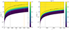 |
Fig. 8. Cumulative contribution of different k values to |


The  are computed with a trapezoidal integral over 200 values of z on a linear grid between zmin and zmax. The integral is performed for discrete values of ℓ, with a logarithmically spaced grid of 100 values of ℓ between ℓmin and ℓmax. Finally, a second-order spline interpolation is used to get the spectra for every integer ℓ.
4.4. Parameters and priors
We list in Table 2 the free parameters used in our forecasts (not including the DM parameters specific to each model, which shall be specified in each Sect. 5). The table also provides the assumed fiducial values and priors. We remind that forecast errors are anyway nearly independent of the chosen fiducial values, especially for the ΛCDM parameters, which have nearly Gaussian posteriors. The first five parameters are the cosmological parameter of the standard ΛCDM model. The following six parameters describe the baryonic feedback model implemented in BCemu. The last 12 nuisance parameters account for linear bias in each bin and intrinsic alignment parameters.
List of free parameter, fiducial values, and top-hat prior ranges used in all our runs.
We use a flat prior on each of these parameters. For the first three BCemu parameters and the two intrinsic alignment parameter, we pass explicit prior edges to ensure that these parameters remain a range making sense physically. For the other parameters, as long as we only perform parameter inference with the Metropolis-Hastings algorithm, it is strictly equivalent to pass to MontePython some very remote prior edges – such that the chains never reach the prior boundaries – or to require the code to use non-informative priors (abbreviated as n.i. in Table 2), in which case the code achieves the same feature automatically. We note that our chains never reach the prior edges passed for the intrinsic alignement parameters, so we are effectively using non-informative priors also for 𝒜IA, ηIA.
Finally, theoretical predictions depend on a few additional parameters that are usually kept fixed because the set of free nuisance parameters from Table 2 are sufficient to account for the uncertainty on the model. For intrinsic alignment, we fix the parameter βIA defined in Eq. (39) to βIA = 2.17; for baryonic feedback, we fix the BCemu parameters μ = 1, γ = 2.5, δ = 7, η = 0.2.
5. Results and discussion
5.1. Cold plus warm dark matter
Main results. For the CWDM model, we perform forecasts using the free parameters  and fwdm introduced in Sect. 2.1. Our fiducial values and priors are summarised in Table 3 for these parameters and Table 2 for all other free parameters. The fiducial model is chosen to be a pure ΛCDM model. As was already stated in Sect. 2.1, we use a linear prior on the mass and a logarithmic prior on the WDM fraction (that is, a flat priors on its logarithm). The latter choice allows us to explore the constraining power of Euclid for very small WDM fractions (see also Schneider et al. 2020). This limit is particularly interesting to study with Euclid since, in this case, Euclid bounds can be competitive with respect to Lyman-α bounds (Hooper et al. 2022).
Indeed, Lyman-α data probe smaller scales than WL and GC surveys, and can in principle better constrain models with a large mass. However, when the WDM fraction is small, the effect of WDM on the power spectrum is also small. Then, it could be unconstrained by Lyman-α data, and if WDM is light enough its effects can manifest themselves on relatively large scales. In this case, the precise measurement of the power spectrum at larger scales with Euclid remains decisive.
Our main results are summarised in Fig. 9, where we show the marginalised 95% credible intervals for fwdm and mwdm. The horizontal axis can be interpreted as the thermal WDM mass (bottom axis) or as the Dodelson–Widrow mass (top axis, see Sect. 2.1 for details). The different colours of the contours mark the different probes that have been used to obtain the constraints. These contours are already marginalised over all other cosmological and nuisance parameters (including baryonic feedback parameters). For each of the six cases shown in Fig. 9, we ran 36 chains summing up to ∼1.4 millions of steps (MS) in each optimistic case or ∼2.6 MS in each pessimistic case. The Gelman-Rubin convergence criterium (Gelman & Rubin 1992) reached about |R − 1|∼0.002 for most parameters, with a worse value of ∼0.008 for a few parameters.
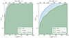 |
Fig. 9. Left: Edges of the 95% credible interval on the WDM mass mwdm and fraction fwdm for the CWDM model, with pessimistic assumptions and three data combinations: WL alone, WL plus GC from the photometric survey (3 × 2pt), and 3 × 2pt combined with Planck CMB data. For the 3 × 2pt and 3 × 2pt + Planck data sets, baryonic feedback has been assumed to affect the WL power spectrum but not the GC power spectrum. The posterior is marginalised over other cosmological parameters, baryonic feedback parameters, and nuisance parameters (accounting for bias uncertainty and intrinsic alignment). The model is equivalent to pure ΛCDM towards the lower horizontal axis (small fwdm) and right vertical axis (large mwdm). The forecast assumes a flat prior on the mass of thermal WDM (lower axis) and a logarithmic prior on the WDM fraction (left axis), but we show the relation to Dodelson–Widrow masses in the upper axis (see Sect. 2.1 for definitions). Right: Same with optimistic assumptions. |
The constraints from WL are considerably looser (by about a factor five) in the pessimistic rather than optimistic case. Indeed, in the pessimistic case, the WL data is only fitted up to ℓmax = 1500, while models with a thermal mass of a few hundreds of keV only affect larger multipoles. As long as one sticks to pessimistic assumptions, adding information from GC (in the photometric survey) and on clustering-lensing correlations (3 × 2pt) makes a small difference, because in this case the clustering information is taken into account only up to ℓmax = 750. The addition of CMB data from Planck also has a very small impact, given that CMB is sensitive to the clustering properties of pressureless DM (including WDM) only at second order in perturbations, through CMB lensing effects – as was explained in Voruz et al. (2014). Figure 9 shows that in the pessimistic case, Euclid 3 × 2pt + Planck data have a potential to rule out masses  (95%CL) in the extreme case where these particles make up the totality of DM, or
  for fwdm = 0.1 (95%CL). We note that even with pessimistic assumptions, the WDM mass can be constrained even for WDM fractions slightly below 0.1, while current bounds from high-resolution Lyman-α data cannot distinguish models with fwdm = 0.1 from the pure ΛCDM limit (Hooper et al. 2022).
The picture drastically improves when one assumes optimistic settings with ℓmax = 5000 for WL and ℓmax = 1500 for GC. The data are then able to probe the presence of WDM with a much smaller value of the maximum free-streaming scale; that is, a larger mass. For the same WDM fraction, using WL data alone, the mass bounds become approximately five times tighter in the optimistic case. Despite of its limitation to ℓmax ≤ 1500, GC data turns out to be very sensitive to the suppression induced by WDM even with a large mass, such that the 3 × 2pt probe is about twice more sensitive than the WL probe alone. However, the combination with Planck data makes no difference also in that case – at least when the mock data is assumed to account for a pure CDM model. The reason is that, for the large WDM masses that remain compatible with the data, the maximum free-streaming scale of WDM is very low, such that even CMB lensing is unaffected by the suppression induced by WDM. In the optimistic case, the Euclid 3 × 2pt probe has a potential to rule out all WDM masses with  for fwdm = 1 and
  for fwdm = 0.1. It can constrain the mass even when fwdm is as low as a few times 10−2; in other words, when only a few percent of the total DM is warm. This region of parameter space is far from current Lyman-α bounds, and even future Lyman-α surveys are unlikely to probe such small WDM fractions.
It is still unclear whether the final Euclid sensitivity will be closer to that of our pessimistic or optimistic forecast. At least, we expect that these two forecasts are bracketing the true constraining power of the future data. We shall see that, compared to other non-minimal DM models discussed in the next sections, CWDM is particularly sensitive to the choice of a cut-off multipole ℓmax. This is due to the step-like nature of the effect of WDM on the matter power spectrum: up to a given wavenumber, the ΛCDM and CWDM models are strictly equivalent, and then the power drops. This means that the constraining power of a data set on the CWDM parameters depends more on the minimum scale (and thus maximum multipole and redshift) included in the analysis than on the actual error bars on the power spectrum. As was discussed above, this is particularly true for large values of fwdm; for tiny WDM fractions, the precision with which the power spectrum is constrained remains crucial.
Importance of baryonic feedback. In Fig. 10, we evaluate the impact of different assumptions concerning baryonic feedback effects. We compare the bounds derived from the 3 × 2pt probe only under three assumptions. The baseline case (orange contours) is the same as in our previous discussion and in Fig. 9: the six nuisance parameters describing baryonic feedback are marginalised over, and baryonic feedback is assumed to affect only the WL probe; that is, the total matter power spectrum. The grey contours are derived assuming instead that baryonic feedback affects the two probes (WL and GC) in the same way: in other words, the same BCemu corrections are applied to the total matter and galaxy power spectra. Finally, the magenta contours were obtained with fixed rather than marginalised baryonic feedback parameters: they account for the unrealistic situation in which baryonic feedback effects would be perfectly known, given some independent measurements.
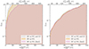 |
Fig. 10. Left: Same as Fig. 9, but only for the 3 × 2pt dataset and with different assumptions on baryonic feedback (BF): fixed BF (magenta), BF affecting only the WL power spectrum (orange), or BF affecting both the WL and GC power spectra (grey). The “truth” is expected to lay between the latter two cases (orange and grey), which give anyway very similar results. Right: Same with optimistic assumptions. |
In principle, introducing more freedom in baryonic physics may result in looser constraints on WDM parameters due to parameter degeneracies. On the other hand, it is not obvious that such degeneracies are present due to the different shape of the effects imprinted by either WDM or baryons, not only as a function of scale but also as a function of redshift. In particular, the redshift dependence of the DM-induced suppression is reversed compared to the one from baryonic effects; its amplitude gets smaller at smaller redshift, due to non-linear clustering and mode-mode coupling, while overall the opposite is true for baryons, at least in most of the redshift range probed by Euclid.
We first compare the orange and magenta contours. In the pessimistic case (left panel), we find that introducing more freedom in the baryonic model and marginalising over baryonic feedback parameters does degrade a bit the bounds on WDM parameters. However, this is no longer true in the optimistic case, which proves that the information contained in the data at large mutipoles is sufficient to disentangle between the physical effects of WDM and baryonic feedback. This underlines the wealth of cosmological information encoded in the deep non-linear regime of the power spectrum.
We now switch to the comparison between the orange and grey contours. The impact of baryonic feedback on the galaxy power spectrum is not understood and modelled as well as its impact on the total matter powers spectrum. However, as was discussed in Sect. 3.5, we expect baryonic effects to be smaller in the galaxy powers spectrum – or at least not bigger. Thus, the true sensitivity of Euclid should lay somewhere between the forecasts corresponding to the grey and orange contours. However, these contours are very close to each other in both pessimistic and optimistic cases. This is likely due to the reverse redshift dependence of WDM and baryonic effects, which allows GC data to discriminate between them. Such a test validates the bounds on CWDM parameters obtained in the previous paragraphs with baryonic feedback included only in the WL probe.
Comparison with current bounds. It is interesting to compare the expected sensitivity of Euclid to current bounds on CWDM parameters obtained by Hervas-Peters et al. (2024) using an existing WL survey, the Kilo Degree Survey (KiDS – see Asgari et al. 2021). We start by comparing the sensitivity of the Euclid WL probe alone with that of KiDS. A fair comparison requires similar priors. However, the KiDS analysis assumes logarithmic priors on both the WDM mass and fraction, with slightly different prior edges than in our previous analysis. Given that Bayesian credible intervals do depend on priors, especially when constraining some parameters describing a model extension that is not required by the data, we repeat some of our forecasts with different top-hat priors matching exactly the ones of KiDS: log10fwdm ∈ [log10(0.005), log10(1)] and ![$ \log_{10} (m_{\mathrm{wdm}}^{\mathrm{thermal}}/\mathrm{keV}) \in [\log_{10}(10), \, \log_{10}(1.5)] $](/articles/aa/full_html/2025/01/aa51611-24/aa51611-24-eq130.gif) . The results are shown in Fig. 11.
. The results are shown in Fig. 11.
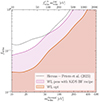 |
Fig. 11. Comparison of our Euclid forecasts for the WL-only probe with current bounds from KiDS. In this particular case, we switch to the same top-hat prior on |


In the pessimistic case, we find that the Euclid sensitivity is not so different from that of KiDS. This result may sound surprising, given the much larger number of galaxy images expected from Euclid. There are two reasons for this.
The first reason is that, as was explained before, in the case of CWDM, the bounds depend a lot on the minimum scale (or maximum wavenumber kmax) included in the analysis, more than on the error bar on the measured power spectrum. It also depends on the maximum redshift of the data, since the signature of WDM is more clear at high redshift and partially washed out at small redshift. We note also that a given multipole ℓ probes smaller wavenumbers at high redshift, as was shown in Eq. (31). In the KiDS analysis and in our Euclid forecast with pessimistic assumptions, the data is conservatively cut at ℓmax = 1500. Thus, within the redshift range covered by both experiments, the maximum wavenumber at each redshift kmax(ℓmax, z) is the same, and the sensitivity to WDM is roughly similar despite of the smaller Euclid error bars. For instance, the highest redshift bin of KiDS peaks around z ∼ 1.1, probing up to k ∼ 1 h Mpc−1. Euclid adds information at higher redshift, with the highest redshift bin peaking around z ∼ 1.7, but at such a high redshift the multipole ℓmax = 1500 projects only to k ∼ 0.5 h Mpc−1, such that the information gain on the CWDM model is marginal. We note that the arguments presented in this paragraph are only valid in the case of the Euclid pessimistic case and for the CWDM model, which has the same power spectrum as ΛCDM up to some large wavenumber k (given by the free-streaming scale). For instance, we shall see that for the 1b-DDM model Euclid is much more constraining than KiDS even with pessimistic assumption because, in that case, the power spectrum contains information on the DM parameters on larger scales/smaller wavenumbers.
A second reason is that, in our analysis, we marginalise over six baryonic feedback parameters, including the three νℬ parameters accounting for a drift of the main feedback parameters ℬ with redshift. In the KiDS analysis, the three ℬ parameters are instead assumed to be redshift-independent. However, the effect of WDM on the matter power spectrum is redshift-dependent (it decreases when the redshift decreases due to mode-mode coupling). Thus, in our analysis, it is easier to cancel the effect of WDM with a shift in the baryonic feedback parameter, and there is more degeneracy between the WDM and baryonic parameters. This tends to lower our forecasted sensitivity and to compensate the fact that Euclid measurements of the lensing power spectrum are expected to be much more accurate. In Fig. 11, we choose to present the results of the Euclid pessimistic forecast with the same treatment as in KiDS analysis of Hervas-Peters et al. (2024); that is, with only three free baryonic feedback parameters, while in the Euclid optimistic forecast we stick to our more conservative baseline treatment with a marginalisation over six parameters ℬ and νℬ.
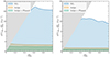 |
Fig. 12. Same as Fig. 9, but for the 1b-DDM model, parameterised by the DDM fraction |


In the optimistic case, we still find that the sensitivity of the Euclid WL probe is approximately three times bigger than that of KiDS, despite of our more conservative modelling of baryonic feedback. In addition, we have already seen that with the inclusion of all the information from the 3 × 2pt probe, we can gain a factor three in sensitivity. All in all, under optimistic assumptions, Euclid could be about ten times more constraining, while providing at the same time some bounds that will be more robust against baryonic feedback effects. Furthermore, we note that the results of our optimistic forecast confirm previous findings from Schneider et al. (2020) using more realistic assumptions for the survey characteristics, especially regarding the tomographic galaxy binning.
5.2. Dark matter with one-body decay
Main results. For the 1b-DDM model, we perform forecasts using the parameter combinations  and
and  defined in Sect. 2.2. The fiducial model is chosen to be a pure ΛCDM model. We showed in Sect. 3.2 that the small-scale suppression induced by 1b-DDM on the linear power spectrum depends only on the product
  , while the non-linear evolution adds a bit of sensitivity to Γddm alone. Thus, the data are expected to provide bounds mainly on the product of the two DDM parameters. Our fiducial values and priors are summarised in Table 4 for these parameters and Table 2 for all other free parameters. The fiducial model is chosen to be a pure ΛCDM model. As was already stated in Sect. 2.2, we use linear priors on
  and
and  . We note that the N-body simulations used by Hubert et al. (2021) to build the emulator were limited to models with a DM lifetime much larger than the age of the Universe, namely τddm ≥ 31.6 Gyr. We thus conservatively include in our run a prior Γddm ≤ 0.0316 Gyr−1. This additional prior excludes a small triangle in the parameter space defined by the priors of Table 4.
Figure 12 presents the 95% confidence level (CL) isocontours of the marginalised posterior for the 1b-DDM parameters inferred from our forecasts for the Euclid WL probe alone (WL), the full Euclid photometric probe (3 × 2pt), and Euclid 3 × 2pt combined with Planck, considering both pessimistic (left panel) or optimistic (right panel) assumptions. The fiducial model, ΛCDM, spans the lower horizontal axis ( ). The shaded grey area restricts the parameter space to the region in which the emulator was trained. The fact that the contour edges remain nearly horizontal is consistent with the fact that 1b-DDM effects depend mainly on the product
  . The small tilting of the contours comes from the fact that non-linear corrections to the 1b-DDM effects do depend on Γddm alone. For each of the six cases shown in Fig. 12, we ran 96 chains summing up to ∼1.6 MS in each optimistic case or ∼3.8 MS in each pessimistic case. The Gelman-Rubin convergence criterium reached about |R − 1|∼0.01 for most parameters, with a worse value of 0.05 for a few parameters.
In the pessimistic case, the WL-only analysis provides a 95%CL bound close to  . Incorporating the 3×2pt data set leads to a substantially stronger bounds, by approximately a factor of 2, such that
  . There is an additional factor of 2 improvement when Planck data are integrated into the analysis, requiring
  . Switching to optimistic assumptions makes a substantial difference for the WL only bound, which shrinks to
  , and an even stronger difference for the 3×2pt bound, which reaches
  . Planck further improves this bound down to
  .
.
The first conclusion emerging from these results is that the photometric GC data has a large constraining power compared to the WL data for this particular model. This is illustrated by the factor 8 improvement when switching from WL to 3×2pt data in the optimistic case. The 2-dimensional likelihood contours shown in the upper panel of Fig. 13 show that, with WL data alone, the parameter  is degenerate with cosmological parameters like, for instance, ns or Ωm. The addition of GC data is beneficial for two reasons: on the one hand, it adds sensitivity to these parameters and helps removing such degeneracies; on the other hand, it directly probes the 1b-DDM effects on the matter power spectrum, up to smaller wavenumbers k than WL data but with better sensitivity.
Another interesting conclusion is that there is a good synergy between the Planck and Euclid probes for this model. We note that, using Planck 2018 data alone, Simon et al. (2022) and Bucko et al. (2023) found  . Thus, the Euclid 3 × 2pt probe alone is already more constraining than Planck. In addition, the combination of the two data sets is significantly more constraining than each data set taken individually. This is usually the consequence of parameter degeneracies being removed by the combination. We get a confirmation of this by looking at the upper and lower panels of Fig. 13. The contours illustrate the existence of correlations between
  and other cosmological parameters. The addition of Planck data resolves these degeneracies and pushes the bounds beyond those from Euclid alone – even if Planck alone is not directly sensitive to such small
  values.
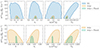 |
Fig. 13. Degeneracies between the 1b-DDM parameter |

Importance of baryonic feedback. In Fig. 14, we show the impact of marginalisation over baryonic feedback parameters, in the same way as we did in Fig. 10 for CWDM. We compare the bounds derived from the 3 × 2pt probe with either marginalised baryonic feedback effects only for the WL probe (orange) or for the full 3 × 2pt probe (grey), or with fixed baryonic feedback effects (magenta).
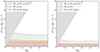 |
Fig. 14. Same as Fig. 10, but for the parameters of the 1b-DDM model. Unlike in the case of CWDM, we find that the various assumptions on baryonic feedback have a big impact on the upper bound on |

There is a qualitative difference between this model and the CWDM case. In the former case, the suppression of the small-scale matter power spectrum is caused by WDM free-streaming during early cosmological times. However, this suppression tends to be washed out at small redshift by non-linear clustering and mode-mode coupling. As redshift decreases, the CWDM matter power spectrum gets gradually closer to that of ΛCDM. This is not the case in the 1b-DDM model, since the DM decay occurs mainly at very late times. Then, the modifications to the non-linear matter power spectrum get more and more pronounced as time passes by – which also tends to be the case for baryonic effects, at least in most of the redshift range probed by Euclid. In principle, this enhances the possibility that 1b-DDM and baryonic effects can compensate each other and that degeneracies are present in parameter space.
As a matter of fact, in the pessimistic case, the bounds are different under the three assumptions. This confirms that baryonic feedback and 1b-DDM effects are partially degenerate, and that the marginalisation over baryonic feedback parameters weakens the bounds. Assuming baryonic feedback effects also on the GC spectrum weakens the bound on  by approximately 25%, such that a conservative estimate in this case is
  (95%CL).
In the optimistic case, we see that the 3 × 2pt data contains enough information to remove the degeneracy between 1b-DDM and baryonic feedback parameters when baryonic feedback is applied to the WL probe only, but not when it is applied also to the GC probe. In this case, the true bound is expected to stand between the one discussed in the previous paragraph,  , and the more conservative one found here,
  (95%CL).
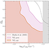 |
Fig. 15. Comparison of bounds from Euclid WL-only (optimistic or pessimistic) and KiDS WL-only (Bucko et al. 2023) on the 1b-DDM parameters, using the same priors for all three cases (logarithmic on the DDM decay rate, linear on the DDM fraction). The shaded grey area restricts the parameter space to the region where τddm = 1/Γddm ≥ 31.6 Gyr in which the emulator was trained. |
Comparison with current bounds. For the 1b-DDM model, Simon et al. (2022) found  when using Planck alone, and no significant improvement when adding information from Type Ia supernovae, baryon acoustic oscillations from a variety of surveys, redshift space distortions from the extended Baryon Oscillation Spectroscopic Survey (eBOSS), and even the full shape of the power spectrum from the Baryon Oscillation Spectroscopic Survey (BOSS). Bucko et al. (2023) find no improvement either when adding KiDS data. Additionally, Bucko et al. (2023) find that KiDS alone only provides a bound of the order of
  , almost one order of magnitude weaker than Planck. This shows that current large-scale structure observations have much less constraining power than current CMB data for this particular model – a situation very different from that of CWDM.
In this context, the sensitivity that will be reached by Euclid according to our forecast is remarkable. Euclid WL-only will improve KiDS WL-only bounds by a factor 4 (pessimistic) or 5 (optimistic)17. The full Euclid 3 × 2pt probe will have the same sensitivity as current CMB data (pessimistic) or improve the bound by a factor 2 to 3 (optimistic). The combined Euclid 3 × 2pt + Planck data will improve over current bounds by a factor 4 (pessimistic) to 8 (optimistic).
We see that Euclid has an even greater potential to improve over current bounds for 1b-DDM than for CWDM. This is related to the shape of the 1b-DDM effects on the matter power spectrum, already displayed in Fig. 2. The survey probes 1b-DDM effects through the entire shape of the power spectrum over the full range of measured linear and non-linear scales. Unlike the CWDM spectrum, the 1b-DDM spectrum is not identical to the ΛCDM one up to a given free-streaming scale. Thus, the constraints on 1b-DDM benefit from the unprecedented accuracy expected from Euclid data over the entire range of scales probed by the survey.
With this model, the sensitivity of Euclid offers an opportunity not only to reconstruct the matter power spectrum accurately over a broad range of scales, but also to disentangle between 1b-DDM and baryonic effects. The strong sensitivity improvement of Euclid versus KiDS is partly due to the fact that there is a significant degeneracy between 1b-DDM and baryonic feedback parameter, which Euclid is able to resolve much better than KiDS. We already explained that baryonic feedback should be more degenerate with 1b-DDM effects than with CWDM effects. Thus, in the CWDM case, there is no such factor and the Euclid sensitivity remains closer to the KiDS one at least in the pessimistic case.
5.3. Dark matter with two-body decay
Main results. For the 2b-DDM model, we perform forecasts using the parameters ( , Γddm, ε) defined in Sect. 2.3, with logarithmic priors defined in Table 5 for these parameters and Table 2 for all other free parameters. As was discussed in Sect. 2.3, at the level of the linear spectrum, 2b-DDM induces a step-like suppression in the power spectrum with an amplitude controlled by (
 , Γddm) and a scale depending on ε. At the non-linear level the effects are more intricate and the suppression depends on all three parameters. The fiducial model of our forecast is chosen to be a pure ΛCDM model.
In Fig. 16 we show the 95%CL contours on each pair of 2b-DDM parameters marginalised over cosmological and nuisance parameters for Euclid WL only, Euclid 3 × 2pt, and 3 × 2pt + Planck data, under pessimistic (left panel) or optimistic (right panel) assumptions. We use the same colour scheme as in Figs. 9 and 12. The fiducial ΛCDM model spans the left and lower axes of each panel. For each of the six cases shown in Fig. 16, we ran 48 chains summing up to ∼1 MS in each optimistic case or ∼1.3 MS in each pessimistic case. The Gelman-Rubin convergence criterium reached about |R − 1|∼0.01 for most parameters, with a worse value of 0.03 for a few parameters.
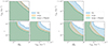 |
Fig. 16. Same as Fig. 9, but for the parameters of the 2b-DDM model. The forecast assumes logarithmic priors on the DDM fraction |


In ( , Γddm) space, the contours follow lines of constant
  . This suggests that for both the 1b-DDM and 2b-DDM models the power spectrum suppression only depends on this product – at least at the linear level. Thus, Euclid can provide joint bounds on
  and ε, while
  or Γddm will be left unconstrained.
We first comment the results of the pessimistic case. With WL only, our forecast returns the 95%CL bound  (marginalised over ε). For
  we find ε < 4 × 10⁻³, while for
  the 2b-DDM model is indistinguishable from ΛCDM at the 95%CL, and ε is unconstrained. With the addition of 3×2pt data, the constraints remain stable. Finally, Planck data is able to alleviate some degeneracies between cosmological parameters and shrink the bounds by about 25%.
In the optimistic case, the WL-only bounds are identical, but the 3 × 2pt bounds shrink by a factor two compared to the 3 × 2pt pessimistic case, or a factor four compared to the WL optimistic case:  (with marginalisation over ε), ε < 1 × 10⁻³ for
  , and the 2b-DDM model is indistinguishable from ΛCDM below
  . In this case, the addition of Planck data makes a difference for the bounds on ε, not because of Planck data being directly sensitive to this parameter, but thanks to the better determination of other parameters. Figure 17 shows how Planck data lift the degeneracy between, for instance, ε and ns. In this case we obtain a bound ε < 0.7 × 10⁻³ for
  .
.
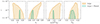 |
Fig. 17. Degeneracies between the 2b-DDM parameter ε and four other cosmological parameters for the optimistic case, in the particular case where |

Importance of baryonic feedback. Figure 18 depicts how different baryonic feedback prescriptions influence the final posteriors, using the same colour and style as Figs. 10 and 14. Like for 1b-DDM, there could be a degeneracy between 2b-DDM and baryonic feedback parameters since both effects tend to grow with time. Indeed, in the 2b-DDM model, the conversion of CDM into WDM particles appears dominantly at very late times and the non-linear matter power spectrum departs more and more from the ΛCDM limit.
However, we find that 2b-DDM effects and baryonic feedback are very weakly correlated. The constraints remain nearly stable when fixing the baryonic feedback parameters instead of marginalising over them, and become slightly weaker when baryonic feedback is applied also to the GC probe. The degradation is at most by a factor two. As a matter of fact, our forecasts predict 95%CL bounds on the 2b-DDM parameter summarised by  (with marginalisation over ε) and ε < 4 × 10⁻³ for
  in the pessimistic case; or
  (with marginalisation over ε) and ε < 2 × 10⁻³ for
  in the optimistic case.
Comparison to current bounds. We believe that our forecast is the first one including as a free parameter the initial fraction  of DDM with two-body decay. Several studies in the past fixed
  . Therefore, in order to compare the expected sensitivity of Euclid to recent results obtained from real observations, we perform a few dedicated forecast with 100% DDM. In Fig. 19, we compare our results to the most recent limits on Γddm and ε from the KiDS survey (Bucko et al. 2024). In this case, we adopt precisely the same top-hat priors on the 2b-DDM parameters as Bucko et al. (2024). We find that Euclid with WL alone can improve over KiDS bounds roughly by a factor 3, while the full 3 × 2pt data would improve over KiDS by one order of magnitude. This improvement is closer to the one observed for 1b-DDM than for CWDM, since a precise measurement of the power spectrum on intermediate (linear and mildly non-linear) scales is crucial to constrain this model, while a better measurement on non-linear scales helps to discriminate decaying DM effects from baryonic feedback effects.
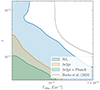 |
Fig. 19. For the 2b-DDM model with |

The 2b-DDM model with  has also been constrained using current Lyman-α data in Fuß & Garny (2023). For very small values of ε, the suppression of the matter power spectrum could occur on such small scales that Lyman-α data would still probe the 2b-DDM effects while Euclid data could not distinguish 2b-DDM from ΛCDM. However, for ε ≥ 10−3, Euclid can probe the effects of 2b-DDM on linear and mildly non-linear scales, and thus can be expected to have more constraining power. This is confirmed by the results of Fuß & Garny (2023), who show that Lyman-α data from BOSS DR14 only constrain Γddm to be smaller than 𝒪(0.1 Gyr−1). This is about one order of magnitude weaker than the predicted Euclid sensitivity.
5.4. ETHOS n = 0
Main results. Our ETHOS n = 0 forecasts use the parameters (adark, ξidr) defined in Sect. 2.4, with logarithmic priors defined in Table 6 for these parameters and Table 2 for all other free parameters. We have seen in Sects. 2.4 and 3.4 that the ETHOS n = 0 model induces a suppression in the power spectrum controlled at the linear level by adarkξidr4 and at the non-linear level by the two ETHOS parameters. The fiducial model of our forecasts is chosen to be a pure ΛCDM model.
In Fig. 20 we show the 95% CL credible interval limits on the free parameters (adark, ξidr) coming from the Euclid WL probe, from the full 3×2pt probe, and from the same in combination with Planck data. For each of the six cases shown in Fig. 20, we ran 48 chains summing up to ∼1 MS in each optimistic case or ∼1.7 MS in each pessimistic case. The Gelman-Rubin convergence criterium reached about |R − 1|∼0.005 for most parameters, with a worse value of ∼0.012 for a few parameters.
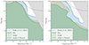 |
Fig. 20. Same as Fig. 9, but for the parameters of the ETHOS n = 0 model. Our forecast assumes logarithmic priors on the interaction strength adark and on the dark-radiation-to-photon temperature ratio ξidr. The model is equivalent to pure ΛCDM in the small adark and/or small ξidr limits. The grey shade excludes the region adarkξidr4 > 0.05 where the non-linear emulator cannot be trusted (see Sect. 3.4). We also show current constraints inferred from Planck, BAO, and BOSS full-shape data by Rubira et al. (2023) – although these authors use different priors. |
In this case, the credible interval limits look slightly wobbly. However, the limits remain stable when pushing the MCMC chains to very high convergence criteria, or when performing multiple independent MCMC runs. Thus, the small oscillations of the contours in Fig. 20 are not caused by MCMC convergence issues but the emulator, which was trained on a slightly too coarse sample of models. In the future, the DMemu emulator will be improved for this model. The oscillations are anyway sufficiently small to allow for a robust qualitative interpretation of our forecast results.
When adark is very small, this model is equivalent to a ΛCDM+ΔNeff model with ΔNeff = 3.85 ξidr4. The radiation excess parameter ΔNeff can be constrained since it affects both the matter power spectrum and CMB anisotropy spectrum in a well-known way (Euclid Collaboration: Archidiacono et al. 2025). In this limit, we expected bounds of the order of ΔNeff < 𝒪(1) (95%CL) from the 3 × 2pt optimistic probe and ΔNeff < 𝒪(0.1) (95%CL) from the combination 3 × 2pt + Planck (Euclid Collaboration: Archidiacono et al. 2025). This translates respectively into log10ξidr < −0.1 (95%CL, 3 × 2pt) and log10ξidr < −0.4 (95%CL, 3 × 2pt + Planck). Our choice of prior, ξidr ∈ [ − 2, −0.4], prevents us from seeing the upper bound in the 3 × 2pt case, but in the case of 3 × 2pt + Planck we can see the upper limit on ξidr just below top axis of each panel in Fig. 20.
For larger values of adark, the model is further constrained by the impact of IDM-IDR interactions on the small-scale matter power spectrum. As was already discussed, at the non-linear level, this effect depends on both adark and ξidr in a non-trivial way. However, for log10(adark/Mpc−1) < 1, we find that the boundary of the preferred region can be approximately fitted by constant values of the combination adark ξidr4 that controls the scattering rate of IDR off IDM.
In the pessimistic case, the most substantial part of the constraining power comes from the WL probe, since further addition of clustering and Planck data do not improve the bounds significantly. In all cases, the bounds for log10(adark/Mpc−1) < 1 can be approximated as adark ξidr4 < 8 × 10⁻⁴ Mpc−1 (95%CL). With the 3 × 2pt probe, the data loses sensitivity to IDM-IDR interactions only for ξidr < 0.06 (i.e. ΔNeff < 5 × 10⁻⁵). We stress that Euclid would not detect such a tiny abundance of dark radiation through the effect of an enhanced radiation density, but through that of DM interactions.
In the optimistic case, the WL-only bound changes marginally, but the 3 × 2pt bound (with or without Planck) shrinks by more than one order of magnitude. For log10(adark/Mpc−1) < 1 the bounds can be approximated by adark ξidr4 < 2 × 10⁻⁵ Mpc−1. With 3 × 2pt information, the data loses sensitivity to the interaction rate only below ξidr < 0.03 (that is, ΔNeff < 3 × 10⁻⁶).
Importance of baryonic feedback. In this case, the impact of baryonic feedback is illustrated in Fig. 21. Interestingly, in the ETHOS n = 0 case, we do not find any hint of degeneracies between the DM and baryonic feedback parameters. In the pessimistic and optimistic cases, the bounds remain roughly stable when the baryonic feedback parameters are fixed rather than marginalised, or when baryonic feedback is applied also to GC. A first explanation comes from the fact that the effect of the ETHOS n = 0 model on the matter power spectrum always starts on linear scales (k ∼ 10−2–10−1 h Mpc−1) which are immune to baryonic feedback. If most of the information on this model resides in such scales, the bounds should indeed be independent from the modelling of baryonic feedback. In addition, like in the CWDM case, the redshift dependence of the DM-induced suppression is opposite to that of baryonic feedback. As a matter of fact, the effect of DM interactions is imprinted on the matter power spectrum at high redshift and subsequently smoothed out by non-linear clustering, while overall baryonic effects tend to grow with time, at least through most of the redshift range probed by Euclid.
Comparison with current bounds. For the same model, using flat priors on ξidr and logarithmic priors on adark, Archidiacono et al. (2019) found adarkξidr4 < 14 × 10−4 Mpc−1 (95%CL) using Planck, BAO, and high-resolution Lyman-α data from the HIRES/MIKE quasar sample. The comparison with our Euclid bound is not straightforward due to the different prior shapes and edges, but indicates that Euclid has a potential to improve over current CMB+Lyman-α bounds by a large factor (a factor 70 according to our predictions in the 3 × 2pt optimistic case). This is actually not so surprising since the ETHOS n = 0 model leaves a signature already on linear scales, much larger than the scales probed by Lyman-α data.
Rubira et al. (2023) also use flat priors on ξidr and logarithmic priors on adark. Their results for IDM interacting with free-streaming IDR is reported in the left panel of their Fig. 4. We extracted from this plot their joint bound on (adark, ξidr) inferred from Planck, BOSS full-shape galaxy spectrum, and KiDS (the latter being implemented as a measurement of S8). We display this bound in Figs. 20 and 21. The comparison with our Euclid forecast should be taken with a grain of salt since the priors are different in the two analyses. However, the main conclusion is that, on the one hand, their bound is similar to our Euclid 3 × 2pt + Planck bound in the limit of large ξidr, which was expected since this bound only reflects the upper limit on ΔNeff from Planck; but on the other hand, for smaller values of ξidr, we find that Euclid is much more sensitive to adark. According to Rubira et al. (2023), the BOSS data loses any sensitivity to adark when ξidr is equal to or smaller than 10−0.8 (that is, ξidr ≤ 0.2, or equivalently ΔNeff ≤ 2 × 10⁻³), while for ξidr = 0.2 Euclid 3 × 2pt data can still constrain the interaction rate to adark < 1 Mpc−1 (95%CL, pessimistic case) or adark < 0.1 Mpc−1 (95%CL, optimistic case).
We conclude that Euclid has a great potential to constrain the ETHOS n = 0 model and to push the bounds well below those from any current experiment.
6. Prospects
Apart from performing additional accuracy tests on the modelling of non-linear clustering and baryonic feedback, our work could be extended in several directions.
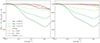 |
Fig. 22. Ratio of the non-linear matter power spectrum at redshift zero for different cosmologies featuring either massive neutrinos or non-minimal DM over that of a reference ΛCDM cosmology with massless neutrinos. In this figure, DM parameters are chosen close to the boundary of the 95% credible intervals in the 3 × 2pt pessimistic (left plot) and optimistic (right plot) case. DM parameter values are given in Table 7. |
First, one could investigate potential degeneracies between massive neutrinos and extended DM models. A priori, we expect this degeneracy to be weak for two reasons. First, neutrino masses and extended DM parameters affect the shape of the matter power spectrum differently and on different scales. Second, they induce a different scale-dependent linear growth rate, and thus a different dependence of the linear and non-linear matter power spectrum on redshift.
To illustrate the first point, we show in Fig. 22 the ratio of the non-linear matter power spectrum at redshift zero for different cosmologies featuring either massive neutrinos or non-minimal DM over that of a reference ΛCDM cosmology with massless neutrinos. In this figure, DM parameters are chosen close to the 95%CL credible interval boundaries found in this work in the pessimistic case (left plot) and optimistic case (right plot). A key point is that the steplike supression induced by neutrino masses always starts at a very small wavenumber (k ≃ 0.003 h Mpc−1). Thus, there is always a wide range of linear scales over which the effect of neutrino masses is large while that of extended DM is insignificant. Data points within this range should allow to discriminate between the summed neutrino mass ∑mν and DM parameters. It would however be useful to check this explicitly with forecasts featuring both types of parameters. This is especially true in the case of the 1b-DDM model, which also suppresses slightly the power spectrum on linear scales, and is thus more likely to exhibit a small level of degeneracy with neutrino masses.
Our approach could also be ported to the study of several other extended DM models with approximately the same number of free model parameters. We recall that in the context of Euclid we are mostly interested in models introducing a step-like (or at least a smooth) suppression of the matter power spectrum, since models introducing a sharp suppression are easier to constrain with Lyman-α data. Still, one could consider cosmologies in which a fraction of DM self-interacts (Boehm et al. 2001; Spergel & Steinhardt 2000; Huo et al. 2018; Kahlhoefer et al. 2019) or scatters over ordinary neutrinos (Boehm & Schaeffer 2005; Serra et al. 2010; Wilkinson et al. 2014; Stadler et al. 2019; Mosbech et al. 2021; Hooper & Lucca 2022; Giarè et al. 2024) or baryons (Chen et al. 2002; Boehm & Schaeffer 2005; Dvorkin et al. 2014; Becker et al. 2021; Ali-Haïmoud et al. 2024). We note that in some cases, like that of DM scattering over baryons, it is unclear whether our assumption of approximate separability between DM scattering effects and baryonic feedback effects would be accurate enough.
7. Summary and conclusions
In summary, we have estimated the sensitivity of the future Euclid photometric probe (i.e. of 3 × 2pt statistics) to the parameters describing four non-minimal DM models. We have run several MCMC forecasts in which the fiducial model assumes plain CDM (with baryonic feedback) while the fitted model includes the effect of non-standard DM (with free baryonic freedback parameters). We have investigated the dependence of the results on various assumptions (cut-off multipole ℓmax, modelling of baryonic feedback, combination with CMB data from Planck). We have also compared the sensitivity predicted by our forecasts with current bounds derived from CMB data, Lyman-alpha data, WL data, and galaxy redshift survey data.
Each of the few non-minimal DM models considered here has a qualitatively different impact on the matter power spectrum. As a matter of fact, we reach significantly different conclusions for each of them in terms of degeneracy with baryonic feedback, constraining power of WL data compared to GC data, or sensitivity of Euclid compared to current bounds. In this section, we put together a compact summary of the most striking conclusions.
For a mixture of cold and warm dark matter (CWDM), the key point is that the power spectrum looks exactly like that of ΛCDM up to a scale fixed by the WDM mass, beyond which a step-like suppression occurs. For large WDM fractions leading to a strong suppression, the mass bounds will always be dominated by data from Lyman-α forests probing smaller scales than Euclid. However, the results of Sect. 5.1 show that Euclid can be very efficient at constraining small WDM masses when the WDM fraction is also small. The Euclid 3×2pt analysis could even bound (or detect) masses of the order of just 𝒪(10) eV (thermal WDM case) or 𝒪(100) eV (Dodelson–Widrow scenario) even if WDM accounts for only 1% of the total DM budget, while current observations are only sensitive to WDM contributing to at least 10% of DM.
The situation is very different with models featuring a mixture of stable and unstable CDM, with the latter undergoing one-body decay into relativistic particles (1b-DDM). In this case, the DM parameters impact the evolution of perturbations up to very large scales, deep in the linear regime. Thus, CMB data is also highly sensitive to the decaying DM fraction fddm and decay rate Γddm – as a matter of fact, on their product fddmΓddm18. However, the results of Sect. 5.2 show that the Euclid 3 × 2pt probe alone could provide twice stronger bounds on fddmΓddm than Planck. In this case, there is a synergy between Euclid and Planck: the combined data sets can resolve parameter degeneracies and strengthen current bounds by a factor eight.
For a mixture of stable and unstable CDM such that the latter undergoes two-body decay into one relativistic and one non-relativistic particle (2b-DDM), the power spectrum is step-like suppressed, a bit like the CWDM case but with a different suppression shape. As a matter of fact, this model can be understood as if a few CDM particles were gradually replaced by WDM particles at late times. In this case, WL and GC surveys are more sensitive to the parameters of the model than Lyman-α data in the limit of small decay rate and large ε; that is, a large velocity dispersion, since in this limit the step-like suppression is small but occurs on relatively large scales. For such models, the results of Sect. 5.3 show that Euclid could improve the bound on the product fddmΓddm by one order of magnitude compared to current WL surveys like KiDS.
For DM interacting with dark radiation at a constant rate (ETHOS n = 0), the power spectrum is suppressed on intermediate and small scales in a more progressive way than for CWDM and 2b-DDM. The suppression looks more like a broken power law than an exponential cut. The forecasts of Sect. 5.4 show that the constraining power of Euclid is particularly strong in this case. Euclid may improve current bounds from Lyman-α and Planck by a factor 70. Through DM interaction effects, Euclid can probe for the first time the limit in which the abundance of dark radiation is very small, namely in the range ΔNeff ∼ [3 × 10⁻⁶, 2 × 10⁻³] that current galaxy surveys do not have the sensitivity to constrain.
Our decision to choose ΛCDM as the fiducial model in each forecast was arbitrary: we could have chosen a fiducial model featuring non-standard DM and compatible with current bounds, and calculated the significance at which Euclid could differentiate this model from ΛCDM. We did not perform such tests due to computational limits, but our forecasts suggest that Euclid has a significant discovery potential. When we find that a 2σ bound from current data could shrink by a factor n with future Euclid data, we get a hint that a DM model described by some parameters saturating the current 2σ limit could be differentiated from ΛCDM roughly at the 2nσ level. Our forecasts show that, in some regions of parameter space, current bounds can improve by one to two orders of magnitude (e.g. a factor 70 in the ETHOS n = 0 case). This shows that there are wide regions in parameter space where Euclid could perform an actual discovery of non-minimal DM properties at a high level of significance.
If an experiment like Euclid provides evidence in favour of a non-minimal DM model, the impact of such a discovery on cosmology will obviously be profound. Several future large-scale structure surveys – for example, from the Square Kilometer Array Observatory (Santos et al. 2015) or Rubin Observatory (Ivezić et al. 2019) – would have an opportunity to check this discovery independently, while our approach to understand and model the process of galaxy and star formation would be deeply impacted. Even if we conservatively assume that Euclid will confirm plain CDM and strengthen all bounds on the parameters of non-minimal DM models, the results will be incredibly interesting, since the new limits will have implications for DM model building and cut into the parameter space of several possible dark sector models.
The step-like amplitude can be approximated as (1 − fwdm)2[D(a0)/D(aeq)]−(3/2)fwdm, where D(a) is the scale-independent linear growth factor of CDM density fluctuations in a pure ΛCDM universe, aeq is the scale factor at radiation-to-matter equality, and a0 is the scale factor today (Boyarsky et al. 2009a).
Since our definition of the reference temperature Tν applies to neutrinos in the instantaneous decoupling limit, in order to be consistent, we need to stick to the same limit when computing the factor mX/(ΩXh2eV). Thus, for this factor, we must use the value 94.1 rather than the slightly smaller value 93.1 that accounts for the mass-to-density ratio of active neutrino.


We use the branch called merging_with_master of the GitHub repository https://github.com/PoulinV/class_decays. This branch is an extension of CLASS v2.7.1..
Here we use CLASSv3.2.0, and we set the parameter of the ETHOS sector, described in Archidiacono et al. (2019), according to: f_idm = 1 to switch on 100% of IDM; nindex_idm_dr = n = 0; idr_nature = free_streaming; a_idm_dr = adark in units of inverse Megaparsecs; and xi_idr = ξidr. Other ETHOS parameters are set to their default value, which means in particular that IDR is assumed to consist of two fermionic degrees of freedom with a statistical factor stat_f_idr = 0.875.
Notice that, in N-GenIC, Type2 particles are assigned thermal velocities as if they were standard neutrinos with three species degenerate in mass. Therefore, in order to correctly account for thermal velocities of WDM, one needs to rescale the mass to assign to the NU_PartMass_in_ev key in the parameter file. The renormalised mass  can be computed through (Bode et al. 2001; Lesgourgues & Pastor 2006)
In our specific case the renormalised mass value is 4290.7 eV.
The code is available at https://github.com/sambit-giri/BCemu.
If this effect was not negligible and was implemented in Eq. (38), it would lead to a redshift-dependent rescaling of Wiγ(z), which could only increase the sensitivity of observations to 1b-DDM parameters. Thus our approximation stays on the conservative side.
We cross-checked this statement by running our Euclid WL forecasts with exactly the same top-hat priors on log10(Γdcdm/Gyr−1) and  as Bucko et al. (2023), see Fig. 15.
In this summary, we use simplified notations. In the core of the paper, the fraction was denoted  , see Sect. 2.2 for precise definitions.
Acknowledgments
We acknowledge computing resources granted by RWTH Aachen University under project thes1340, rwth1411, rwth1437, and rwth1481. We also acknowledge funding from DFG project 456622116 and support from the IRAP and IN2P3 Lyon computing centers. The Euclid Consortium acknowledges the European Space Agency and a number of agencies and institutes that have supported the development of Euclid, in particular the Agenzia Spaziale Italiana, the Austrian Forschungsförderungsgesellschaft funded through BMK, the Belgian Science Policy, the Canadian Euclid Consortium, the Deutsches Zentrum für Luft-und Raumfahrt, the DTU Space and the Niels Bohr Institute in Denmark, the French Centre National d’Etudes Spatiales, the Fundação para a Ciência e a Tecnologia, the Hungarian Academy of Sciences, the Ministerio de Ciencia, Innovación y Universidades, the National Aeronautics and Space Administration, the National Astronomical Observatory of 1930 Japan, the Netherlandse Onderzoekschool Voor Astronomie, the Norwegian Space Agency, the Research Council of Finland, the Romanian Space Agency, the State Secretariat for Education, Research, and Innovation (SERI) at the Swiss Space Office (SSO), and the United Kingdom Space Agency. A complete and detailed list is available on 1935 the Euclid web site (https://www.euclid-ec.org/).
References
- Abdalla, E., Franco Abellán, G., Aboubrahim, A., et al. 2022, JHEAp, 34, 49 [NASA ADS] [Google Scholar]
- Ali-Haïmoud, Y., Gandhi, S. S., & Smith, T. L. 2024, Phys. Rev. D, 109, 083523 [CrossRef] [Google Scholar]
- Anderhalden, D., Schneider, A., Maccio, A. V., Diemand, J., & Bertone, G. 2013, JCAP, 03, 014 [CrossRef] [Google Scholar]
- Angulo, R. E., Zennaro, M., Contreras, S., et al. 2021, MNRAS, 507, 5869 [NASA ADS] [CrossRef] [Google Scholar]
- Aoyama, S., Sekiguchi, T., Ichiki, K., & Sugiyama, N. 2014, JCAP, 07, 021 [Google Scholar]
- Archidiacono, M., Hooper, D. C., Murgia, R., et al. 2019, JCAP, 10, 055 [CrossRef] [Google Scholar]
- Asgari, M., Lin, C.-A., Joachimi, B., et al. 2021, A&A, 645, A104 [NASA ADS] [CrossRef] [EDP Sciences] [Google Scholar]
- Audren, B., Lesgourgues, J., Benabed, K., & Prunet, S. 2013a, JCAP, 02, 001 [Google Scholar]
- Audren, B., Lesgourgues, J., Bird, S., Haehnelt, M. G., & Viel, M. 2013b, JCAP, 01, 026 [CrossRef] [Google Scholar]
- Audren, B., Lesgourgues, J., Mangano, G., Serpico, P. D., & Tram, T. 2014, JCAP, 12, 028 [Google Scholar]
- Becker, N., Hooper, D. C., Kahlhoefer, F., Lesgourgues, J., & Schöneberg, N. 2021, JCAP, 02, 019 [Google Scholar]
- Berezhiani, Z., Dolgov, A. D., & Tkachev, I. I. 2015, Phys. Rev. D, 92, 061303 [NASA ADS] [CrossRef] [Google Scholar]
- Bertone, G., Hooper, D., & Silk, J. 2005, Phys. Rept., 405, 279 [NASA ADS] [CrossRef] [Google Scholar]
- Bird, S., Viel, M., & Haehnelt, M. G. 2012, MNRAS, 420, 2551 [Google Scholar]
- Blas, D., Lesgourgues, J., & Tram, T. 2011, JCAP, 07, 034 [CrossRef] [Google Scholar]
- Bode, P., Ostriker, J. P., & Turok, N. 2001, ApJ, 556, 93 [Google Scholar]
- Boehm, C., & Schaeffer, R. 2005, A&A, 438, 419 [NASA ADS] [CrossRef] [EDP Sciences] [Google Scholar]
- Boehm, C., Fayet, P., & Schaeffer, R. 2001, Phys. Lett. B, 518, 8 [NASA ADS] [CrossRef] [Google Scholar]
- Bond, J. R., & Szalay, A. S. 1983, ApJ, 274, 443 [NASA ADS] [CrossRef] [Google Scholar]
- Bonvin, C., & Durrer, R. 2011, Phys. Rev. D, 84, 063505 [NASA ADS] [CrossRef] [Google Scholar]
- Boyarsky, A., Lesgourgues, J., Ruchayskiy, O., & Viel, M. 2009a, JCAP, 05, 012 [CrossRef] [Google Scholar]
- Boyarsky, A., Lesgourgues, J., Ruchayskiy, O., & Viel, M. 2009b, Phys. Rev. Lett., 102, 201304 [NASA ADS] [CrossRef] [Google Scholar]
- Brinckmann, T., & Lesgourgues, J. 2019, Phys. Dark Univ., 24, 100260 [Google Scholar]
- Bucko, J., Giri, S. K., & Schneider, A. 2023, A&A, 672, A157 [NASA ADS] [CrossRef] [EDP Sciences] [Google Scholar]
- Bucko, J., Giri, S. K., Peters, F. H., & Schneider, A. 2024, A&A, 683, A152 [NASA ADS] [CrossRef] [EDP Sciences] [Google Scholar]
- Buen-Abad, M. A., Marques-Tavares, G., & Schmaltz, M. 2015, Phys. Rev. D, 92, 023531 [Google Scholar]
- Buen-Abad, M. A., Schmaltz, M., Lesgourgues, J., & Brinckmann, T. 2018, JCAP, 01, 008 [Google Scholar]
- Casas, S., Lesgourgues, J., Schöneberg, N., et al. 2024, A&A, 682, A90 [NASA ADS] [CrossRef] [EDP Sciences] [Google Scholar]
- Challinor, A., & Lewis, A. 2011, Phys. Rev. D, 84, 043516 [NASA ADS] [CrossRef] [Google Scholar]
- Chen, X.-L., Hannestad, S., & Scherrer, R. J. 2002, Phys. Rev. D, 65, 123515 [Google Scholar]
- Chisari, N. E., Richardson, M. L. A., Devriendt, J., et al. 2018, MNRAS, 480, 3962 [Google Scholar]
- Chudaykin, A., Gorbunov, D., & Tkachev, I. 2016, Phys. Rev. D, 94, 023528 [NASA ADS] [CrossRef] [Google Scholar]
- Chudaykin, A., Gorbunov, D., & Tkachev, I. 2018, Phys. Rev. D, 97, 083508 [NASA ADS] [CrossRef] [Google Scholar]
- Colombi, S., Dodelson, S., & Widrow, L. M. 1996, ApJ, 458, 1 [NASA ADS] [CrossRef] [Google Scholar]
- Cyr-Racine, F.-Y., Sigurdson, K., Zavala, J., et al. 2016, Phys. Rev. D, 93, 123527 [NASA ADS] [CrossRef] [Google Scholar]
- Dakin, J., Hannestad, S., & Tram, T. 2022, MNRAS, 513, 991 [CrossRef] [Google Scholar]
- Diamanti, R., Ando, S., Gariazzo, S., Mena, O., & Weniger, C. 2017, JCAP, 06, 008 [Google Scholar]
- Dodelson, S., & Widrow, L. M. 1994, Phys. Rev. Lett., 72, 17 [CrossRef] [Google Scholar]
- Dvorkin, C., Blum, K., & Kamionkowski, M. 2014, Phys. Rev. D, 89, 023519 [NASA ADS] [CrossRef] [Google Scholar]
- Enqvist, K., Nadathur, S., Sekiguchi, T., & Takahashi, T. 2015, JCAP, 09, 067 [CrossRef] [Google Scholar]
- Euclid Collaboration (Blanchard, A., et al.) 2020, A&A, 642, A191 [NASA ADS] [CrossRef] [EDP Sciences] [Google Scholar]
- Euclid Collaboration (Archidiacono, M., et al.) 2025, A&A, 693, A58 [NASA ADS] [CrossRef] [EDP Sciences] [Google Scholar]
- Euclid Collaboration (Mellier, Y., et al.) 2025, A&A, in press, https://doi.org/10.1051/0004-6361/202450810 [Google Scholar]
- Euclid Collaboration (Cropper, M. S., et al.) 2025, A&A, in press, https://doi.org/10.1051/0004-6361/202450996 [Google Scholar]
- Euclid Collaboration (Jahnke, K., et al.) 2025, A&A, in press, https://doi.org/10.1051/0004-6361/202450786 [Google Scholar]
- Feng, J. L. 2010, ARA&A, 48, 495 [NASA ADS] [CrossRef] [Google Scholar]
- Feng, J. L., Kaplinghat, M., Tu, H., & Yu, H.-B. 2009, JCAP, 07, 004 [CrossRef] [Google Scholar]
- Franco Abellán, G., Murgia, R., & Poulin, V. 2021, Phys. Rev. D, 104, 123533 [CrossRef] [Google Scholar]
- Franco Abellán, G., Murgia, R., Poulin, V., & Lavalle, J. 2022, Phys. Rev. D, 105, 063525 [CrossRef] [Google Scholar]
- Franco Abellán, G., Herrera, G. C., Martinelli, M., et al. 2024, JCAP, 11, 057 [Google Scholar]
- Fuß, L., & Garny, M. 2023, JCAP, 10, 020 [Google Scholar]
- Gelman, A., & Rubin, D. B. 1992, Stat. Sci., 7, 457 [Google Scholar]
- Giarè, W., Gómez-Valent, A., Di Valentino, E., & van de Bruck, C. 2024, Phys. Rev. D, 109, 063516 [CrossRef] [Google Scholar]
- Giri, S. K., & Schneider, A. 2021, JCAP, 12, 046 [CrossRef] [Google Scholar]
- Giri, S. K., & Schneider, A. 2023, Astrophysics Source Code Library [record ascl:2308.010] [Google Scholar]
- Gluscevic, V., Ali-Haïmoud, Y., Bechtol, K., et al. 2019, Bull. Am. Astron. Soc., 51, 134 [Google Scholar]
- Grandis, S., Aricò, G., Schneider, A., & Linke, L. 2024, MNRAS, 528, 4379 [NASA ADS] [CrossRef] [Google Scholar]
- Haridasu, B. S., & Viel, M. 2020, MNRAS, 497, 1757 [NASA ADS] [CrossRef] [Google Scholar]
- Hervas-Peters, F., Schneider, A., Bucko, J., Giri, S. K., & Parimbelli, G. 2024, A&A, 687, A161 [NASA ADS] [CrossRef] [EDP Sciences] [Google Scholar]
- Holm, E. B., Herold, L., Hannestad, S., Nygaard, A., & Tram, T. 2023, Phys. Rev. D, 107, L021303 [NASA ADS] [CrossRef] [Google Scholar]
- Hooper, D. C., & Lucca, M. 2022, Phys. Rev. D, 105, 103504 [NASA ADS] [CrossRef] [Google Scholar]
- Hooper, D. C., Schöneberg, N., Murgia, R., et al. 2022, JCAP, 10, 032 [Google Scholar]
- Hubert, J., Schneider, A., Potter, D., Stadel, J., & Giri, S. K. 2021, JCAP, 10, 040 [Google Scholar]
- Huo, R., Kaplinghat, M., Pan, Z., & Yu, H.-B. 2018, Phys. Lett. B, 783, 76 [NASA ADS] [CrossRef] [Google Scholar]
- Ichiki, K., Oguri, M., & Takahashi, K. 2004, Phys. Rev. Lett., 93, 071302 [NASA ADS] [CrossRef] [Google Scholar]
- Ivezić, Z., Kahn, S. M., Tyson, J. A., et al. 2019, ApJ, 873, 111 [NASA ADS] [CrossRef] [Google Scholar]
- Joachimi, B., & Bridle, S. L. 2010, A&A, 523, A1 [NASA ADS] [CrossRef] [EDP Sciences] [Google Scholar]
- Joachimi, B., & Schneider, P. 2009, A&A, 507, 105 [NASA ADS] [CrossRef] [EDP Sciences] [Google Scholar]
- Kahlhoefer, F., Kaplinghat, M., Slatyer, T. R., & Wu, C.-L. 2019, JCAP, 12, 010 [Google Scholar]
- Kaiser, N. 1992, ApJ, 388, 272 [Google Scholar]
- Kilbinger, M., Heymans, K., Asgari, M., et al. 2017, MNRAS, 472, 2126 [NASA ADS] [CrossRef] [Google Scholar]
- Knabenhans, M., Stadel, J., Potter, D., et al. 2021, MNRAS, 505, 2840 [NASA ADS] [CrossRef] [Google Scholar]
- Lepori, F., Tutusaus, I., Viglione, C., et al. 2022, A&A, 662, A93 [NASA ADS] [CrossRef] [EDP Sciences] [Google Scholar]
- Lesgourgues, J. 2011, ArXiv e-prints [arXiv:1104.2932] [Google Scholar]
- Lesgourgues, J., & Pastor, S. 2006, Phys. Rep., 429, 307 [Google Scholar]
- Lesgourgues, J., & Tram, T. 2011, JCAP, 09, 032 [CrossRef] [Google Scholar]
- Lesgourgues, J., & Verde, L. 2022, Rev. Neutrinos Cosmol. Rev. Part. Phys, 2022, 083C01 [Google Scholar]
- Lesgourgues, J., Marques-Tavares, G., & Schmaltz, M. 2016, JCAP, 02, 037 [Google Scholar]
- Ma, Z.-M., Hu, W., & Huterer, D. 2005, ApJ, 636, 21 [Google Scholar]
- Maccio, A. V., Ruchayskiy, O., Boyarsky, A., & Munoz-Cuartas, J. C. 2013, MNRAS, 428, 882 [CrossRef] [Google Scholar]
- Mead, A. J., Brieden, S., Tröster, T., & Heymans, C. 2021, MNRAS, 502, 1401 [Google Scholar]
- Mosbech, M. R., Boehm, C., Hannestad, S., et al. 2021, JCAP, 03, 066 [Google Scholar]
- Murgia, R., Merle, A., Viel, M., Totzauer, M., & Schneider, A. 2017, JCAP, 11, 046 [Google Scholar]
- Murgia, R., Iršič, V., & Viel, M. 2018, Phys. Rev. D, 98, 083540 [NASA ADS] [CrossRef] [Google Scholar]
- Nygaard, A., Tram, T., & Hannestad, S. 2021, JCAP, 05, 017 [Google Scholar]
- Oldengott, I. M., Boriero, D., & Schwarz, D. J. 2016, JCAP, 08, 054 [Google Scholar]
- Pandey, K. L., Karwal, T., & Das, S. 2020, JCAP, 07, 026 [Google Scholar]
- Parimbelli, G., Scelfo, G., Giri, S. K., et al. 2021, JCAP, 12, 044 [Google Scholar]
- Potter, D., Stadel, J., & Teyssier, R. 2017, Comput. Astrophys. Cosmol., 4, 2 [NASA ADS] [CrossRef] [Google Scholar]
- Poulin, V., Serpico, P. D., & Lesgourgues, J. 2016, JCAP, 08, 036 [Google Scholar]
- Rubira, H., Mazoun, A., & Garny, M. 2023, JCAP, 01, 034 [Google Scholar]
- Santos, M., Bull, P., Alonso, D., et al. 2015, Advancing Astrophysics with the Square Kilometre Array (AASKA14), 19 [Google Scholar]
- Schneider, A. 2015, MNRAS, 451, 3117 [NASA ADS] [CrossRef] [Google Scholar]
- Schneider, A., & Teyssier, R. 2015, JCAP, 12, 049 [Google Scholar]
- Schneider, A., Teyssier, R., Stadel, J., et al. 2019, JCAP, 03, 020 [CrossRef] [Google Scholar]
- Schneider, A., Refregier, A., Grandis, S., et al. 2020, JCAP, 04, 020 [Google Scholar]
- Schneider, A., Giri, S. K., Amodeo, S., & Refregier, A. 2022, MNRAS, 514, 3802 [NASA ADS] [CrossRef] [Google Scholar]
- Schöneberg, N., Franco Abellán, G., Pérez Sánchez, A., et al. 2022, Phys. Rept., 984, 1 [CrossRef] [Google Scholar]
- Serra, P., Zalamea, F., Cooray, A., Mangano, G., & Melchiorri, A. 2010, Phys. Rev. D, 81, 043507 [Google Scholar]
- Simon, T., Franco Abellán, G., Du, P., Poulin, V., & Tsai, Y. 2022, Phys. Rev. D, 106, 023516 [NASA ADS] [CrossRef] [Google Scholar]
- Sitzmann, V., Martel, J. N. P., Bergman, A. W., Lindell, D. B., & Wetzstein, G. 2020, Adv. Neural Inf. Process. Syst., submitted [arXiv:2006.09661] [Google Scholar]
- Smith, R. E., Peacock, J. A., Jenkins, A., et al. 2003, MNRAS, 341, 1311 [Google Scholar]
- Spergel, D. N., & Steinhardt, P. J. 2000, Phys. Rev. Lett., 84, 3760 [NASA ADS] [CrossRef] [Google Scholar]
- Springel, V., White, S. D. M., Jenkins, A., et al. 2005, Nature, 435, 629 [Google Scholar]
- Stadler, J., Bœhm, C., & Mena, O. 2019, JCAP, 08, 014 [Google Scholar]
- Takahashi, R., Sato, M., Nishimichi, T., Taruya, A., & Oguri, M. 2012, ApJ, 761, 152 [Google Scholar]
- Takahashi, R., Nishimichi, T., Namikawa, T., et al. 2020, ApJ, 895, 113 [NASA ADS] [CrossRef] [Google Scholar]
- Tanidis, K., & Camera, S. 2019, MNRAS, 489, 3385 [NASA ADS] [CrossRef] [Google Scholar]
- Tanidis, K., Cardone, V. F., Martinelli, M., et al. 2024, A&A, 683, A17 [NASA ADS] [CrossRef] [EDP Sciences] [Google Scholar]
- Tram, T., Brandbyge, J., Dakin, J., & Hannestad, S. 2019, JCAP, 03, 022 [Google Scholar]
- van Daalen, M. P., McCarthy, I. G., & Schaye, J. 2020, MNRAS, 491, 2424 [Google Scholar]
- Vattis, K., Koushiappas, S. M., & Loeb, A. 2019, Phys. Rev. D, 99, 121302 [NASA ADS] [CrossRef] [Google Scholar]
- Verde, L., Treu, T., & Riess, A. G. 2019, Nat. Astron., 3, 891 [Google Scholar]
- Voruz, L., Lesgourgues, J., & Tram, T. 2014, JCAP, 03, 004 [Google Scholar]
- Wilkinson, R. J., Boehm, C., & Lesgourgues, J. 2014, JCAP, 05, 011 [Google Scholar]
- Workman, R. L., Burkert, V. D., Crede, V., et al. 2022, PTEP, 2022, 083C01 [Google Scholar]
- Xiao, L., Zhang, L., An, R., Feng, C., & Wang, B. 2020, JCAP, 01, 045 [Google Scholar]
- Yoo, J., & Zaldarriaga, M. 2014, Phys. Rev. D, 90, 023513 [NASA ADS] [CrossRef] [Google Scholar]
- Yoo, J., Fitzpatrick, A. L., & Zaldarriaga, M. 2009, Phys. Rev. D, 80, 083514 [NASA ADS] [CrossRef] [Google Scholar]
All Tables
Specifications used in our mock Euclid photometric likelihood in the pessimistic (pess.) and optimistic (opt.) cases.
List of free parameter, fiducial values, and top-hat prior ranges used in all our runs.
All Figures
|
Fig. 1. Ratio of the linear (solid lines) and non-linear (dashed lines) power spectra of several CWDM models to that of a pure ΛCDM model with the same cosmological parameters, parameterised by the fraction fwdm and the rescaled mass x. The other parameters (Ωdm, Ωb, h, As, ns) are kept fixed. All spectra are computed today (z = 0). These plots cover all the cases in which WDM has a Fermi–Dirac distribution possibly rescaled by a factor χ, including the limits of the thermal WDM (χ = 1) and Dodelson–Widrow (Twdm = Tν) models. In the latter case x coincides with the physical mass. The non-linear spectra are predicted by the emulator introduced in Sect. 3.1 and plotted up to the maximum wavenumber at which this emulator is trusted. |
| In the text | |
|
Fig. 2. Ratio of the linear (solid lines) and non-linear (dashed lines) power spectra of several 1b-DDM models to that of a pure ΛCDM model with the same cosmological parameters, parameterised by the fraction |
| In the text | |
|
Fig. 3. Ratio of the linear (solid lines) and non-linear (dashed lines) power spectra of several two-body DDM models to that of a pure ΛCDM model with the same cosmological parameters, parameterised by the fraction |
| In the text | |
|
Fig. 4. Ratio of the linear (solid lines) and non-linear (dashed lines) power spectra of several free-streaming ETHOS n = 0 models to that of a pure ΛCDM model with the same cosmological parameters, parameterised by the dark-radiation-to-photon temperature ratio ξidr and interaction strength adark. The effects are displayed in the basis (ξidr, adark ξidr4) to show that the combination adark ξidr4, which gives the scattering rate of IDR off IDM, controls the amplitude of the small-scale suppression of the linear matter power spectrum. The other parameters ( |
| In the text | |
|
Fig. 5. Left: Effect of neglecting the WDM thermal velocities in CWDM simulations with fwdm = 0.2 and |
| In the text | |
|
Fig. 6. Effect of 1b-DDM parameters on the linear (solid) and non-linear (dashed) matter power spectrum. Left: Effect of varying the decay rate Γddm with a fixed fraction |
| In the text | |
|
Fig. 7. Left: Ratio of the interaction rate between IDM and IDR (Γidm − dr) and comoving Hubble rate (ℋ) as a function of the dark-radiation-to-photon temperature ratio ξidr and interaction strength adark, computed at the redshift zini = 49 at which the N-body simulations used to construct the ETHOS emulator are initialised. We display the contours of equal ratio as solid white lines and highlight the threshold value of 0.1 in black. We further depict the region with adark = 10 Mpc−1 (dashed grey) and ξidr = 0.25 (dash-dotted grey). Right: Power spectrum suppression 𝒮ETHOS(k, z) predicted by the emulator for parameters chosen along each of the two grey lines of the left panel. |
| In the text | |
|
Fig. 8. Cumulative contribution of different k values to |
| In the text | |
|
Fig. 9. Left: Edges of the 95% credible interval on the WDM mass mwdm and fraction fwdm for the CWDM model, with pessimistic assumptions and three data combinations: WL alone, WL plus GC from the photometric survey (3 × 2pt), and 3 × 2pt combined with Planck CMB data. For the 3 × 2pt and 3 × 2pt + Planck data sets, baryonic feedback has been assumed to affect the WL power spectrum but not the GC power spectrum. The posterior is marginalised over other cosmological parameters, baryonic feedback parameters, and nuisance parameters (accounting for bias uncertainty and intrinsic alignment). The model is equivalent to pure ΛCDM towards the lower horizontal axis (small fwdm) and right vertical axis (large mwdm). The forecast assumes a flat prior on the mass of thermal WDM (lower axis) and a logarithmic prior on the WDM fraction (left axis), but we show the relation to Dodelson–Widrow masses in the upper axis (see Sect. 2.1 for definitions). Right: Same with optimistic assumptions. |
| In the text | |
|
Fig. 10. Left: Same as Fig. 9, but only for the 3 × 2pt dataset and with different assumptions on baryonic feedback (BF): fixed BF (magenta), BF affecting only the WL power spectrum (orange), or BF affecting both the WL and GC power spectra (grey). The “truth” is expected to lay between the latter two cases (orange and grey), which give anyway very similar results. Right: Same with optimistic assumptions. |
| In the text | |
|
Fig. 11. Comparison of our Euclid forecasts for the WL-only probe with current bounds from KiDS. In this particular case, we switch to the same top-hat prior on |
| In the text | |
|
Fig. 12. Same as Fig. 9, but for the 1b-DDM model, parameterised by the DDM fraction |
| In the text | |
|
Fig. 13. Degeneracies between the 1b-DDM parameter |
| In the text | |
|
Fig. 14. Same as Fig. 10, but for the parameters of the 1b-DDM model. Unlike in the case of CWDM, we find that the various assumptions on baryonic feedback have a big impact on the upper bound on |
| In the text | |
|
Fig. 15. Comparison of bounds from Euclid WL-only (optimistic or pessimistic) and KiDS WL-only (Bucko et al. 2023) on the 1b-DDM parameters, using the same priors for all three cases (logarithmic on the DDM decay rate, linear on the DDM fraction). The shaded grey area restricts the parameter space to the region where τddm = 1/Γddm ≥ 31.6 Gyr in which the emulator was trained. |
| In the text | |
|
Fig. 16. Same as Fig. 9, but for the parameters of the 2b-DDM model. The forecast assumes logarithmic priors on the DDM fraction |
| In the text | |
|
Fig. 17. Degeneracies between the 2b-DDM parameter ε and four other cosmological parameters for the optimistic case, in the particular case where |
| In the text | |
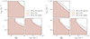 |
Fig. 18. Same as Fig. 10, but for the parameters of the 2b-DDM model. |
| In the text | |
|
Fig. 19. For the 2b-DDM model with |
| In the text | |
|
Fig. 20. Same as Fig. 9, but for the parameters of the ETHOS n = 0 model. Our forecast assumes logarithmic priors on the interaction strength adark and on the dark-radiation-to-photon temperature ratio ξidr. The model is equivalent to pure ΛCDM in the small adark and/or small ξidr limits. The grey shade excludes the region adarkξidr4 > 0.05 where the non-linear emulator cannot be trusted (see Sect. 3.4). We also show current constraints inferred from Planck, BAO, and BOSS full-shape data by Rubira et al. (2023) – although these authors use different priors. |
| In the text | |
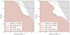 |
Fig. 21. Same as Fig. 10, but for the parameters of the ETHOS n = 0 model. |
| In the text | |
|
Fig. 22. Ratio of the non-linear matter power spectrum at redshift zero for different cosmologies featuring either massive neutrinos or non-minimal DM over that of a reference ΛCDM cosmology with massless neutrinos. In this figure, DM parameters are chosen close to the boundary of the 95% credible intervals in the 3 × 2pt pessimistic (left plot) and optimistic (right plot) case. DM parameter values are given in Table 7. |
| In the text | |
Current usage metrics show cumulative count of Article Views (full-text article views including HTML views, PDF and ePub downloads, according to the available data) and Abstracts Views on Vision4Press platform.
Data correspond to usage on the plateform after 2015. The current usage metrics is available 48-96 hours after online publication and is updated daily on week days.
Initial download of the metrics may take a while.