| Issue |
A&A
Volume 664, August 2022
|
|
|---|---|---|
| Article Number | A179 | |
| Number of page(s) | 19 | |
| Section | Cosmology (including clusters of galaxies) | |
| DOI | https://doi.org/10.1051/0004-6361/202243539 | |
| Published online | 30 August 2022 | |
The BEHOMO project: Λ Lemaître-Tolman-Bondi N-body simulations⋆
1
INAF – Osservatorio Astronomico di Trieste, 34131 Trieste, Italy
e-mail: This email address is being protected from spambots. You need JavaScript enabled to view it.
2
IFPU – Institute for Fundamental Physics of the Universe, 34151 Trieste, Italy
3
Núcleo Cosmo-ufes & Departamento de Física, Universidade Federal do Espírito Santo, 29075-910, Vitória, ES, Brazil
4
INFN – Sezione di Trieste, 34100 Trieste, Italy
5
PPGCosmo, Universidade Federal do Espírito Santo, 29075-910 Vitória, ES, Brazil
6
Dipartimento di Fisica, Sezione di Astronomia, Universitá di Trieste, 34143 Trieste, Italy
7
Dipartimento di Fisica e Astronomia “Augusto Righi”, Alma Mater Studiorum Universitá di Bologna, 40129 Bologna, Italy
Received:
14
March
2022
Accepted:
25
May
2022
Abstract
Context. Our universe may feature large-scale inhomogeneities and anisotropies that cannot be explained by the standard model of cosmology, that is, the homogeneous and isotropic Friedmann-Lemaître-Robertson-Walker metric, on which the Λ cold dark matter model is built, may not accurately describe observations. Currently, there is not a satisfactory understanding of the evolution of the large-scale structure on an inhomogeneous background.
Aims. We have launched the cosmology beyond homogeneity and isotropy (BEHOMO) project to study the inhomogeneous Λ Lemaître-Tolman-Bondi model with the methods of numerical cosmology. Understanding the evolution of the large-scale structure is a necessary step in constraining inhomogeneous models with present and future observables and placing the standard model on more solid ground.
Methods. We perform Newtonian N-body simulations, whose accuracy in describing the background evolution is checked against the general relativistic solution. The large-scale structure of the corresponding Λ cold dark matter simulation is also validated.
Results. We obtain the first set of simulations of the Λ Lemaître-Tolman-Bondi model ever produced. The data products consist of 11 snapshots between redshift 0 and 3.7 for each of the 68 simulations that have been performed, together with halo catalogs and lens planes relative to 21 snapshots, between redshift 0 and 4.2, for a total of approximately 180 TB of data.
Conclusions. We plan to study the growth of perturbations at the linear and nonlinear level, gravitational lensing, and cluster abundances and proprieties.
Key words: large-scale structure of Universe / gravitation / cosmology: theory / cosmological parameters
Data can be obtained upon request. Further information is available at https://valerio-marra.github.io/BEHOMO-project
© V. Marra et al. 2022
 Open Access article, published by EDP Sciences, under the terms of the Creative Commons Attribution License (https://creativecommons.org/licenses/by/4.0), which permits unrestricted use, distribution, and reproduction in any medium, provided the original work is properly cited.
This article is published in open access under the Subscribe-to-Open model. This email address is being protected from spambots. You need JavaScript enabled to view it. to support open access publication.
1. Introduction
Several anomalous signals in cosmological observables have emerged since the establishment of the Λ cold dark matter (CDM) model as the standard model of cosmology more than two decades ago. Particularly relevant here are the Hubble crisis, the cosmic-microwave-background (CMB) anomalies, and the cosmic dipoles and bulk flows (see Perivolaropoulos & Skara 2022, and references therein). Such signals indicate anomalies that challenge the ΛCDM model and its foundations. One may then ask if the universe features large-scale inhomogeneities and anisotropies that cannot be explained by the standard paradigm, or, equivalently, if the homogeneous and isotropic Friedmann-Lemaître-Robertson-Walker (FLRW) metric, on which the ΛCDM model is built, does not accurately describe observations. This constitutes the motivation for studying the universe without assuming homogeneity and isotropy, trying instead to reconstruct the metric directly from observations (Stebbins 2012).
According to the standard reasoning, the validity of the FLRW metric is a consequence of the observed isotropy of the universe and the Copernican principle, which states that humans are not special observers. Here, however, we are not advocating that the universe is inhomogeneous and humans are special, rather that the scale at which there is homogeneity and isotropy could be larger than the commonly thought ≈100 Mpc (Scrimgeour et al. 2012; Laurent et al. 2016; Ntelis et al. 2017), that is, the cosmological principle may be valid at grander scales (see Sect. 8 of Abdalla et al. 2022). We note that this scenario is not necessarily at odds with the observed approximate isotropy of the CMB (see the discussion of the Ehlers-Geren-Sachs theorem in Rasanen 2009).
Inhomogeneous cosmology is undeniably a challenging subject as it would require a considerable theoretical and numerical effort to study its phenomenology. The absence of an FLRW background makes it particularly difficult to study early universe physics and predict, for instance, the CMB power spectrum. Therefore, in order to present a viable program, here we consider a subclass of inhomogeneous cosmologies. The basic requirement is that, at early times, one recovers a near-FLRW metric such that the standard inflationary paradigm is maintained and the physics that leads to the CMB remains basically unchanged. In other words, we consider a standard cosmology endowed with a nonstandard large-scale structure that is dominated by growing modes. This requirement effectively imposes restrictions on the free functions that characterize inhomogeneous metrics, considerably simplifying both analysis and statistical inference. We name these inhomogeneous models “early-FLRW cosmologies”.
Clearly, early-FLRW cosmologies are constrained by CMB observations. Indeed, as shown by Valkenburg (2012a), perturbations at the last scattering surface of present-day contrast ≈0.1 and size ≈1 Gpc would produce temperature fluctuations of ΔT ≈ 50μK on a scale of ≈5°. Similarly, too strong structures along the line of sight at z ≲ 1 would be detected via the integrated Sachs-Wolfe (ISW) effect : a present-day contrast ≈0.1 and size ≈300 Mpc would produce temperature fluctuations of order ΔT ≈ 20 − 30 μK (see, for instance, Zibin 2021; Nadathur et al. 2014). To put this figure in perspective, the famous cold spot of the CMB features ΔT ≈ 70μK across a 5° region (Vielva 2010). Therefore, early-FLRW cosmologies are, at most, mildly nonlinear large-scale perturbations of the FLRW metric.
The inhomogeneities of early-FLRW cosmologies may be regarded as a particular type of primordial non-Gaussianity. Their distinguishing features are nonstandard amplitudes and phases. Indeed, they are characterized by bulk flows and coherent perturbations in the energy content of the universe at arbitrarily large scales. In other words, large-scale homogeneity and isotropy are violated by the phases of these extra modes, so observations depend on the position of the observer and the notion of an average FLRW observer ceases to be meaningful (Kolb et al. 2010). Specifically, large-scale inhomogeneities alter observations both because they affect photon geodesics and because the observer’s local space-time is perturbed. Of course, this is also true within the ΛCDM model, but there the size of this effect is constrained by the standard perturbation spectrum. For example, cosmic variance on local measurements of H0 is expected to be at most 1% within ΛCDM (Camarena & Marra 2018).
The background evolution of early-FLRW cosmologies, that is, the evolution neglecting standard primordial perturbations, can be studied via exact solutions of general relativity. If considering more general scenarios, one can use linear-perturbation theory or simulations via codes that use general relativistic (GR) perturbation theory such as gevolution (Adamek et al. 2016) and CONCEPT (Dakin et al. 2021). A general consequence of spatial gradients is the occurrence of background shear, that is, the fact that the universe expands in an anisotropic way.
The scenario becomes more involved once primordial perturbations are added to the inhomogeneous background. First, there is the issue of the backreaction of small-scale perturbations on the average dynamics of the (possibly inhomogeneous) universe. Here, we assume that backreaction gives a negligible effect, as tested via GR simulations (Giblin et al. 2016; Bentivegna & Bruni 2016; Adamek et al. 2019; Macpherson et al. 2019). An overview of the backreaction proposal is given in Sect. 2.12. Second, because of spatial gradients, the standard primordial perturbations are coupled at first order so that standard perturbation theory does not hold in an inhomogeneous background. Within the spherical Lemaître-Tolman-Bondi (LTB) space-time, this issue has been tackled by Zibin (2008), Clarkson et al. (2009), Dunsby et al. (2010), February et al. (2014), and Meyer et al. (2015) via the numerical integration of the system of coupled equations and by Nishikawa et al. (2012) via second-order perturbation theory. It was concluded that the effect of spatial gradients could have an impact on the growth of perturbations. However, a full perturbation theory and modeling is missing, hampering comparison with perturbation observables – the focus of current and next-generation surveys such as the Dark Energy Survey (DES, Abbott et al. 2022)1, the Dark Energy Spectroscopic Instrument (DESI, Aghamousa et al. 2016)2, the Javalambre Physics of the Accelerating universe Astrophysical Survey (J-PAS, Bonoli et al. 2021)3, the Legacy Survey of Space and Time (LSST, Abate et al. 2012)4, Euclid (Amendola et al. 2018)5, and the Square Kilometre Array (SKA, Braun et al. 2015)6.
Here we introduce the cosmology beyond homogeneity and isotropy (BEHOMO) project. We propose a program that aims at addressing the modeling of linear and nonlinear perturbations and understanding the rich phenomenology of early-FLRW cosmologies. In order to do so, the basic idea is to apply the methods of numerical cosmology, as pioneered by Alonso et al. (2010, 2012). The ultimate goal is to confront arbitrarily early-FLRW inhomogeneous models with data from next-generation surveys. The idea is to adopt Newtonian N-body simulations, whose accuracy in describing the background evolution shall be checked with GR codes. The basic methodology is to feed state-of-the-art N-body codes such as GADGET (Springel et al. 2021) with special early-FLRW initial conditions so that early-FLRW cosmologies can reach the same resolution of standard ΛCDM simulations in approximately the same CPU time (except for the most nonlinear cases). This program will bring the field of inhomogeneous cosmologies into the era of precision cosmology, on par with the ΛCDM model.
In this paper we present the first suite of simulations for the simplest possible early-FLRW cosmologies: spherically symmetric ΛLTB models. We use the LTB metric to model a spherical inhomogeneity on top of the standard ΛCDM model. Though still a toy model, on a first approximation one can regard the spatial gradients of the ΛLTB model as an archetype for more realistic structures with background shear. We consider a set of high-resolution simulations with varying inhomogeneity size and depth, the two main physical parameters that describe such a structure. This will allow us to understand and model the effect of spatial gradients on the evolution of perturbations, which is necessary to confront inhomogeneous cosmologies with perturbation observables such as redshift-space distortions, weak lensing, and cluster abundances. As said earlier, the grand goal is to study and then constrain the phenomenology of these beyond-ΛCDM inhomogeneities with observations (Valkenburg et al. 2014; Redlich et al. 2014; Camarena et al. 2021).
In this presentation paper we review the ΛLTB model in Sect. 2, discuss the numerical details of the inhomogeneous N-body simulations and their data products in Sect. 3, present the results of the simulations in Sect. 4, and discuss the road map of the BEHOMO project7 in Sect. 5. Regarding notation: we use “LTB metric” as opposed to “FLRW metric” but “ΛLTB model” as opposed to “ΛCDM model”; quantities without explicit radial dependence are relative to the FLRW background if pertinent; bold denotes vectors; and c = 1 is assumed unless stated otherwise.
2. The ΛLTB model
We consider early-FLRW ΛLTB models, that is, the ΛCDM model endowed with a spherical inhomogeneity, which is described via the exact LTB solution of Einstein’s equations. As we are considering early-FLRW cosmologies, this model is fully specified by the radial profile function, whose basic parameters are the effective radius and depth of the inhomogeneity.
In this section, after reviewing the formalism and dynamics of the LTB metric, we connect with the more standard Newtonianly perturbed FLRW metric and discuss the historical relevance of LTB models, putting coherently together results from many different papers.
2.1. Metric
In the comoving and synchronous gauge, the spherically symmetric LTB metric can be written as
 (1)
(1)
where the longitudinal (a∥) and perpendicular (a⊥) scale factors are related by a∥ = (a⊥r)′, and a prime denotes partial derivation with respect to the coordinate radius r. We also adopt the alternative notation Y(t, r)≡a⊥r so that Y′≡a∥. In the limit k→ constant and a⊥ = a∥ = a, we recover the FLRW metric, but here k(r) is a free function named the LTB curvature function.
The two scale factors define two different Hubble rates:
 (2)
(2)
 (3)
(3)
where a dot denotes partial derivation with respect to the coordinate time t. This has important implications when confronting these models with observations. For example, cosmic chronometers probe dz/dt and so H∥ (see Eq. (26)); radial baryon acoustic oscillations (BAOs) also probe H∥, but angular BAOs and supernovae probe the angular and luminosity distance, respectively, and so a⊥ and H∥ (see Eqs. (26)–(29)). Combining these observables can then place interesting constraints on the background shear (Garcia-Bellido & Haugboelle 2009):
![Mathematical equation: $$ \begin{aligned} \Sigma (t,r) = \frac{2}{3} \Big [ H_{\parallel }(t,r) - H_{\perp }(t,r) \Big ] \,. \end{aligned} $$](/articles/aa/full_html/2022/08/aa43539-22/aa43539-22-eq4.gif) (4)
(4)
As said earlier, the spatial gradient of the ΛLTB model is an archetype for more realistic structures.
2.2. Dynamics
By solving Einstein’s equations for an irrotational dust source in the presence of a cosmological constant Λ, one obtains the equivalent of the Friedmann equation, which can be written as (Enqvist 2008; Marra & Paakkonen 2012, Appendix B)
 (5)
(5)
where ρΛ = Λ/8πG, and the last term is the Euclidean average of the spatial Ricci scalar (the trace of the Ricci tensor of the spatial metric on the hypersurface of constant t):
 (6)
(6)
 (7)
(7)
where the Euclidean volume element – obtained by setting k = 0 in Eq. (1) – is used:
 (8)
(8)
The fact that a Euclidean rather than proper average is used leads to backreaction, as discussed in Sect. 2.13. Similarly, Eq. (5) features the Euclidean average of the local matter density, ρm:
 (9)
(9)
 (10)
(10)
 (11)
(11)
where the LTB mass function F(r), a constant of integration, is another free function that gives the total gravitating mass up to the shell of coordinate radius r. The local density ρm satisfies the continuity equation  , where θ = H∥ + 2H⊥ is the expansion scalar. We note that, as the source is pressureless dust, without pressure gradients, both F(r) and k(r) do not depend on t. The case of the Lemaître metric with pressure is presented in Yamamoto et al. (2016).
Similarly to FLRW, one can interpret the curvature function as related to the total energy per unit of mass of the shell at coordinate radius r:
 (12)
(12)
where the first term of the energy function E is the kinetic energy per unit of mass of the shell r, the second term is the potential energy per unit of mass due to the total gravitating mass up to the shell r, and the third term is the usual contribution from the cosmological constant (as in the de Sitter-Schwarzschild metric). We note that, thanks to spherical symmetry, one is able to define a potential energy also in cases far away from nearly Newtonian ones and that the potential energy is related to the curvature (Bondi 1947).
Next, similarly to FLRW, one can rewrite Eq. (5) using the equivalent of the density parameters in FLRW:
 (13)
(13)
where the subscript 0 denotes a quantity evaluated at the present time, t0, and
 (14)
(14)
 (15)
(15)
 (16)
(16)
which satisfy Ωm(t, r)+ΩΛ(t, r)+Ωk(t, r) = 1.
2.3. Free functions and gauge fixing
Equation (13) can be used to determine the age of the universe at a radial coordinate r:
 (17)
(17)
where the big bang function tbb(r) is another arbitrary function, which sets the time since the big bang (a⊥ = 0). If it were  , the initial singularity would have happened at different times for different shells so that large inhomogeneities would develop in the past, as can be seen from Eq. (9) with Y → 0. This clearly signals the presence of decaying modes, which would be strongly in contradiction with the inflationary paradigm and are excluded by the choice of a simultaneous big bang (Silk 1977; Biswas et al. 2007; Zibin 2008).
Summarizing, we have seen that the LTB inhomogeneity is specified by three arbitrary functions, F(r), k(r), and tbb(r), which are related, together with a⊥0, by Eq. (17) so that one is not independent. Moreover, one can always make a redefinition of the radial coordinate. Common gauge fixing are F(r)∝r3 or a⊥0= constant. It is then clear that one can choose tbb(r) and k(r) as the free functions that specify the model.
Each gauge fixing has pros and cons. For example, F(r)∝r3 excludes the possibility that there is pure vacuum in some radial interval, and the moment of shell crossing – the time at which Y′ = 0 so that grr = 0 – clearly depends on the gauge adopted. The numerical codes that we use, VoidDistances2020 (Valkenburg 2012b) and FalconIC (Valkenburg & Hu 2015), adopt the choice  , where M0 is an arbitrary mass scale.
2.4. Compensated inhomogeneity profile
As discussed earlier, we consider early-FLRW cosmologies in agreement with the standard scenario of inflation and, therefore, we set
 (18)
(18)
We are then left with the curvature function. Here, we consider the case of an LTB inhomogeneity that matches exactly with the FLRW metric at the finite radius rb and not only asymptotically. This simplified approach is convenient for the purposes of this work because it allows us to robustly simulate the LTB inhomogeneity inside of a bigger FLRW box. The curvature function is modeled according to the monotonic profile:
 (19)
(19)
where rb is the coordinate radius of the spherical inhomogeneity, kb and kc are the curvature outside and at the center of the inhomogeneity, respectively, and W3 is the function
 (20)
(20)
The function Wn(x) interpolates from 1 to 0 when x varies from 0 to 1 while remaining differentiable, which implies that that k(r) is C∞ everywhere. It is dmWn/dxm|0 = 0 for 0 < m < n, so that there is no cusp at the center. In the limit n → ∞, Wn(x) approaches the top-hat function.
For r ≥ rb the curvature profile equals the curvature kb of the background FLRW such that for r ≥ rb one exactly recovers the background ΛCDM model: a⊥ = a∥ = a. We can then define the local density contrast according to:
 (21)
(21)
and the (integrated) mass density contrast according to
 (22)
(22)
where we used the Euclidean average in agreement with Eq. (5). We note that Δ(t, r = 0) = δ(t, r = 0). We denote with δ0 the central contrast today, which is directly related to kc (see Eq. (35) for the linear relation at early times).
We also note that, because of the matching, it is by construction Δ(t, r = rb) = δ(t, r = rb) = 0. This implies that the central underdensity or overdensity at 0 ≤ r < rt, determined by the curvature kc at the center, is automatically compensated by a surrounding overdense or underdense shell at rt ≤ r < rb, where rt is the transition radius at which δ = 0. A compensating overdense or underdense region is an expected feature of the standard large-scale structure: voids are surrounded by sheets and filaments, and superclusters by voids. We note that it is rt = rt(t), as in Eq. (9) the volume element at the denominator is time dependent.
2.5. Physical and light cone distances
The comoving radial coordinate, r, because of the freedom in redefining it, does not possess physical meaning. On the other hand, the proper distance between r1 and r2 (dt2 = dΩ2 = 0 in Eq. (1)) is
 (23)
(23)
where the approximation holds for
 (24)
(24)
Inside the inhomogeneity (r < rb) the curvature radius is  , while outside the LTB patch it is
  . We consider models with kb = 0 so that the corrections to Eq. (23) will be due only to the inhomogeneity. We will see that these corrections are also negligible for gigaparsec-scale inhomogeneities (E ≪ 1; see Fig. 1).
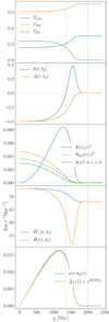 |
Fig. 1. LTB quantities as a function of the FLRW comoving coordinate, χ, at the present time, t0. The two dotted lines mark the positions of the shells relative to rt and rb. See Sect. 2.7. |
Using Eq. (23) we can then define the corresponding FLRW comoving coordinate as
 (25)
(25)
so that the FLRW and LTB physical distances coincide (note that Y′≠0). Thanks to the adopted matching condition, it is χ = r for r ≥ rb. The coordinate χ is the one used in the numerical simulations.
Observationally, the time, t, and radius, r, as a function of the redshift, z, are determined on the past light cone of the central observer by the differential equations for radial null geodesics (see, e.g., Chung & Romano 2006; Enqvist 2008):
 (26)
(26)
 (27)
(27)
with the initial conditions t(0) = t0 and r(0) = 0. The area (dA) and luminosity (dL) distances are given by
 (28)
(28)
 (29)
(29)
2.6. Model parameters
The ΛLTB model is specified by the usual background FLRW parameters, that is, the Hubble constant H0, the total matter density parameter Ωm, and the curvature parameter Ωk, by the standard perturbation parameters, that is, the baryon density parameter Ωb, the optical depth τ, the helium fraction YP, the effective number of relativistic species Neff, the total neutrino mass ∑mν, and the amplitude of the primordial power spectrum As and its tilt ns, and, finally, by the LTB parameters, that is, the central curvature kc and the inhomogeneity radius rb. While numerically the profile is specified via kc, we adopt, in its stead, the derived parameter δ0, which is the contrast today at the center of the inhomogeneity and is more intuitive to most cosmologists. Table 1 summarizes all the parameters and their fiducial values.
Parameters specifying the ΛLTB model.
2.7. Example of inhomogeneity
Figure 1 shows the relevant functions for the case of a central underdensity of present-day contrast δ0 = −0.4 and comoving radius rb = 2000 Mpc, and the fiducial BEHOMO cosmology of Table 1. In particular, one can note that the interior of the inhomogeneity is an open FLRW universe (first panel from the top), that there is a compensating overdensity that surrounds the inner underdensity (second panel), and how the longitudinal Hubble rate deviates from the perpendicular Hubble rate where there is a spatial gradient (fourth panel). Also shown, for later use, are the linear and nonlinear Newtonian potentials together with the energy function (third panel), and the change in redshift induced by the inhomogeneity, together with the peculiar velocity defined in Eq. (38) (last panel). Figure 2 shows the relevant functions on the light cone as compared to their ΛCDM equivalent.
From Fig. 1 one can see that an inhomogeneity with a central underdensity of contrast δ0 = −0.4 could solve the discrepancy between local (Riess et al. 2021) and high-redshift (Aghanim et al. 2020) determinations of the Hubble constant: H0 goes from the background value of 68 km s−1Mpc−1 to the local value of 73 km s−1Mpc−18 This is the so-called local void scenario. However, this scenario is ruled out by other observations. Camarena et al. (2021, 2022) constrained the ΛLTB model using the latest available data from the CMB, BAOs, type Ia supernovae, the local H0, cosmic chronometers, Compton y-distortion, and the kinetic Sunyaev-Zeldovich (kSZ) effect and showed that an underdensity around the observer as modeled within the ΛLTB model cannot solve the H0 tension. Appendix A reports the latest constraints by Camarena et al. (2021) using the LTB parameters δ0 and rb that we adopt here.
2.8. Newtonianly perturbed FLRW metric
One can regard the LTB inhomogeneity as a perturbation on top of the ΛCDM model. Here, we connect the formalism of the previous sections with that of the Newtonianly perturbed FLRW metric:
 (30)
(30)
where, for simplicity, we assumed a flat background FLRW metric. This will be particular relevant as N-body simulations are in an FLRW background (see the discussion regarding the N-body gauge in Fidler et al. 2017). This analysis will also be useful to highlight observational effects specific to ΛLTB inhomogeneities. As we will see, in the case of sub-horizon inhomogeneities it is Φ ≪ 1.
By linearizing the LTB metric and considering a linear gauge transformation, one finds that the Newtonian potential for r < rb is (Biswas & Notari 2008; Van Acoleyen 2008)
 (31)
(31)
and Φlin = 0 for r ≥ rb, where the potential is written as a function of the LTB coordinate. Hereafter, the subscript “lin” refers to the fact that a linear gauge transformation is used; the potential is always linear, that is, a first-order perturbed quantity. We also note that Φlin is constant in time, as should be for a linear matter perturbation in a matter-dominated universe. This description should be accurate at z ≳ 10. The corresponding linear density contrast is
 (32)
(32)
![Mathematical equation: $$ \begin{aligned} \nabla ^{2}\Phi _{\rm lin}(r)&=\Phi ^{\prime \prime }_{\rm lin} + 2 \frac{\Phi^\prime _{\rm lin}}{r} = -\frac{3}{5} \left[ \frac{E^\prime ( r)}{ r} + \frac{E( r)}{ r^2} \right] \,, \end{aligned} $$](/articles/aa/full_html/2022/08/aa43539-22/aa43539-22-eq38.gif) (33)
(33)
 (34)
(34)
where quantities without explicit radial dependence are relative to the FLRW background. We took the derivative with respect to r instead of the Newtonian gauge coordinate  , but the difference is second order. Using Eq. (34) together with Eqs. (12) and (19), one can find the initial evolution of the central density contrast as a function of the central curvature, kc:
 (35)
(35)
One could use second-order perturbation theory to improve upon this linear description (Matarrese et al. 1998). However, given that, in general, the LTB inhomogeneity may feature nonlinear contrasts9, we now consider the potential as obtained via a nonlinear gauge transformation  and
and  , which, following Van Acoleyen (2008), is implicitly defined for r < rb by
 (36)
(36)
 (37)
(37)
and by  and
and  for r ≥ rb, where the peculiar velocity is
![Mathematical equation: $$ \begin{aligned} { v} (\tilde{t}, \tilde{r})&= \dot{Y}(t,r) - \dot{a} (t) \, \tilde{r}=\dot{Y}(t,r)- H(t)\, Y(t,r) \nonumber \\&= Y(t,r) \big [ H_{\perp }(t,r) - H(t) \big ] \,. \end{aligned} $$](/articles/aa/full_html/2022/08/aa43539-22/aa43539-22-eq48.gif) (38)
(38)
This gauge transformation will keep terms up to Φ, E ∼ v2 and is valid for sub-horizon inhomogeneities. From Eq. (36) one sees that  , that is, the coordinate χ defined in Eq. (25) is indeed the one associated with the Newtonian gauge and, therefore, the one adopted by N-body simulations.
One can then use Eqs. (36)–(37) to change the LTB metric of Eq. (1) into the Newtonian gauge of Eq. (30) so as to find the potential Φ. Alternatively, one may proceed by inverting the Poisson equation:
![Mathematical equation: $$ \begin{aligned} \nabla ^{2}\Phi (\tilde{r}) = \frac{1}{\tilde{r}^2} \big (\tilde{r}^2 \Phi^\prime \big )^\prime = 4 \pi G a^2 \left[ \frac{F^\prime }{4 \pi Y^2 Y^\prime } \!-\! \frac{3 }{8 \pi G} \left(H^2- \frac{\Lambda }{3} \right) \right] , \end{aligned} $$](/articles/aa/full_html/2022/08/aa43539-22/aa43539-22-eq50.gif) (39)
(39)
where the derivatives are with respect to the variable of the corresponding function. In particular, it is  , so that one can integrate on
  and obtain
 (40)
(40)
where the constant of integration has been chosen in order to have Φ′(rb) = 0 and the potential is expressed with respect to the LTB coordinate. Integrating again on  , one finally has
 (41)
(41)
 (42)
(42)
where Yb = arb. We note that Φ(rb) = 0 and that we expressed the potential with respect to the LTB coordinate. It is interesting to note ∇2Φ gives exactly the LTB contrast in LTB coordinates while the gauge transformation is only valid up to 𝒪(Φ). Figure 1 (third panel, green solid curve) shows how the potential of Eq. (41) decays during the cosmological-constant dominated phase as compared to the linear-gauge potential of Eq. (31) during matter domination. Also shown (green dot-dashed line) is the linear perturbation result Φ(t, r) = Φlin(r)D(t)/a(t), where D is the ΛCDM growth function normalized at the matter-dominated epoch. The agreement with Eq. (41) is perfect for linear LTB perturbations but it overestimates the value of the potential in the case of the nonlinear underdensity of Fig. 1.
It is easy to verify that Φ′ in Eq. (40) reduces to that of Eq. (32) at early times:
 (43)
(43)
 (44)
(44)
where we used Eq. (12) in the first equality, Eq. (31.14, Kaiser 2014) in the third equality and F ≃ 4πY3ρm(t)/3 in the last equality. Moreover, using the result after the second equality, one has
 (45)
(45)
in agreement with the expected matter-dominated result (Coles & Lucchin 2002, Eq. (18.1.9)).
2.9. Observables in terms of the Newtonian potential
If one uses the metric functions of the LTB metric of Eq. (1) then the effects of the inhomogeneities are exactly taken into account. However, it is important to discuss and review how the Newtonian potential affects observables. Indeed, the total potential will consist of the sum of the LTB potential and the potential relative to the primordial Gaussian perturbations, and the LTB potential may have observational effects in regimes in which the standard Gaussian potential is inconsequential.
A well-known result is that the redshifts of photons are affected by perturbations according to (see, for example, Bonvin et al. 2006)
 (46)
(46)
where the vector n gives the direction of the source S with velocity vS with respect to the observer O with velocity vO. In the following, we only consider the contribution from the LTB potential, but there are of course also contributions from standard-model perturbations. The change in redshift can be interpreted as the sum of three effects.
First, there is the differential Doppler shift due to the peculiar motion of source and observer. This contribution is zero if the observer and the source are placed outside the inhomogeneity or (one of them) at its center. Otherwise, one expects a contribution that is proportional to v ∼ YΔH ∼ rb/rhor where rhor = H−1 is the Hubble radius. This contribution is large for gigaparsec-scale inhomogeneities and can significantly alter the luminosity distance–redshift relation; it was indeed used to fit supernova data without dark energy in the void scenario (see Sect. 2.11 for a historical note). Figure 1 (bottom panel) shows this effect for an underdensity of contrast δ0 = −0.4 and comoving radius rb = 2000 Mpc. Also shown is the peculiar velocity as defined in Eq. (38). One can see that most of the change in redshift can indeed be attributed to a Doppler shift.
The second term gives the so-called Sachs-Wolfe effect, that is, the differential gravitational redshift due to the gravitational potentials at the source’s and observer’s positions (Sachs & Wolfe 1967). This contribution is zero if the observer and the source are placed outside the inhomogeneity. Otherwise, by comparing Eqs. (12) and (38) it is easy to see that E ∼ Ẏ2/ − Y2H2/2 ∼ −v2/2 so that the potential of Eq. (31) is quadratic in the velocities, Φ ∝ v2. It then follows that Φ ∝ (rb/rhor)2 and the Sachs-Wolfe effect is subdominant with respect to the Doppler shift. Again from the analysis of Fig. 1 (bottom panel), one can see that δz/1 + z ≃ −4 × 10⁻⁵ at rb, significantly smaller than the Doppler shift that occurs for source inside the inhomogeneity.
Finally, the last term is the ISW effect, which is present only if the (first-order) gravitational potential evolves with time and is responsible for a nontrivial correlation between CMB anisotropies and the large-scale structure. At high redshift, 10 ≲ z ≲ 100, the standard model is very close to the flat matter-dominated Einstein-de Sitter model. It is then well-known that the (linear) potential is time independent so that the ISW contribution is zero. At later times, however, there are two contributions. First, the universe enters the cosmological constant-dominated phase: this is responsible for the (linear) ISW effect. Second, structures may enter the nonlinear regime so that the so-called Rees-Sciama (RS) effect cannot be neglected. As discussed in Cai et al. (2010), the nonlinear RS correction to the ISW effect acts differently for over and underdensities. Biswas & Notari (2008) explicitly showed that these contributions are suppressed according to ∝(rb/rhor)3.
For the mildly nonlinear large structures here considered, one expects that RS is subdominant with respect to ISW (Sakai & Inoue 2008). In this case, the potential decays according to the linear ISW modeling:
 (47)
(47)
where the (nonlinear) potential is obtained via Eq. (41) and the ISW growth factor, G, is
![Mathematical equation: $$ \begin{aligned} G(z) =(1+z) H(z) [1-f(z)] D(z) \,, \end{aligned} $$](/articles/aa/full_html/2022/08/aa43539-22/aa43539-22-eq62.gif) (48)
(48)
where D is the linear growth function,  with γ = 6/11 + 15/113(1 − Ωm(t)) is the linear growth rate (Wang & Steinhardt 1998), and P(r) encodes the information on the inhomogeneity profile. A thorough discussion is available in Nadathur et al. (2012) and Flender et al. (2013).
As thoroughly discussed in Hui & Greene (2006), a perturbation in the redshift affects the luminosity distance. As we have seen, the LTB metric features possibly large contributions from peculiar velocities that are instead negligible in the standard paradigm. This means that proper care has to be adopted when analyzing these models on the light cone. The other important effect to consider is lensing, which modifies the observed flux of an object without changing its redshift. However, in this case, the total effect will be directly computed by binning mass in a suitable number of lens planes. Indeed, the total lensing effect is the sum of the contribution of the LTB potential with the one of the Gaussian perturbations’ potential, and these two components make up the various lens planes.
2.10. Scale invariance
As the dynamical equation (Eq. (5)) does not present gradients, the dynamics of the LTB model is scale invariant. This is due to spherical symmetry and the fact that the energy-momentum tensor is dust. The former implies a vanishing magnetic Weyl tensor and consequently no gravitational waves; the latter implies no pressure and so no sound waves. In other words, no direct communication can exist between neighboring worldlines and for this reason such space-times were dubbed “silent” (Matarrese et al. 1993; Bruni et al. 1995). In particular, pressure gradients would transfer energy between shells and make the energy function E and mass function F time dependent (see Marra & Paakkonen 2012).
Formally, starting from the solution of Eq. (5) for a given rb, one can obtain a scaled inhomogeneity with coordinate  and size
  . The Friedmann-like equation is then
 (49)
(49)
where we adopted the gauge fixing  and the functions relative to the scaled inhomogeneity are defined according to
 (50)
(50)
 (51)
(51)
 (52)
(52)
 (53)
(53)
 (54)
(54)
 (55)
(55)
 (56)
(56)
 (57)
(57)
 (58)
(58)
Starting from one numerical solution, one can then obtain a family of solutions by varying λ.
We note that velocities, and thus Doppler effects, are proportional to λ, explaining why one needs a large inhomogeneity to sizably change the luminosity distance–redshift relation, as in the void scenario discussed in Sect. 2.11. Also, the energy function and the potential scale quadratically with the size so that one expects strong features in the power spectrum of large inhomogeneities.
2.11. A historical note on LTB void models
The LTB model has been studied extensively in the literature as an alternative to dark energy. The relevant case was of an observer sitting near the center of a gigaparsec-scale underdensity. It is easy to understand how such an observer would see apparent acceleration: most of our cosmological observables are confined to the light cone and, hence, temporal changes can be associated with spatial changes along photon geodesics. The LTB void model then replaces “faster expansion now than before” with “faster expansion here than there”. Mathematically, the directional derivative on the past light cone follows d/dt ≈ ∂/∂t − ∂/∂r and the accelerating expansion can be explained by H′(r) < 0 (Enqvist 2008). For 15 years the LTB model was phenomenologically viable, although suffered the extreme fine-tuning of the observer’s position (see Marra & Notari 2011; Bolejko et al. 2011; Clarkson 2012 and references therein). More importantly, it constituted perhaps the only example of a paradigm that departed abruptly from ΛCDM. This allowed cosmologists to ask new questions and develop new methodologies.
However, in 2011, two papers ruled out the LTB model, which already showed problems when confronted with more and more data (Garcia-Bellido & Haugboelle 2008; Moss et al. 2011; Biswas et al. 2010). Zhang & Stebbins (2011) (see also Zibin & Moss 2011; Bull et al. 2012) showed that void models without decaying modes produce an excessively large kSZ signal, and Zibin (2011) showed that void models with sizable decaying modes (which could possibly have a small kSZ signal) are ruled out because of y-distortion.
Despite the strong evidence against void models as alternatives to dark energy, one has to point out that those studies considered a homogeneous radiation field. In other words, inhomogeneities were present only in the matter component. Clarkson & Regis (2011) and Lim et al. (2013) considered the more consistent scenario of inhomogeneities also in the radiation and showed that this could alter kSZ and y-distortion predictions.
2.12. The backreaction proposal
Because of the nonlinear nature of general relativity, the average of the solution of Einstein’s equations for an inhomogeneous metric is not the solution of Einstein’s equations for the average of the metric, that is, the operation of smoothing does not commute with solving Einstein’s equations, ⟨Gμν(gαβ)⟩ ≠ Gμν(⟨gαβ⟩). Consequently, the Friedmann equation – valid for a homogeneous universe – features corrections in the form of extra sources (see Ellis et al. 1984, which is considered the backreaction manifesto).
In the early 2000s, right after the first analyses indicating the acceleration of the universe’s expansion by Riess et al. (1998) and Perlmutter et al. (1999), it was asked if dark energy could actually be explained via the extra sources generated by the nonlinear smoothing, that is, via the backreaction of small-scale inhomogeneities into the large-scale dynamics of the universe. This scenario would elegantly explain the biggest problem of dark energy, of why it appears at z ≈ 1. The answer would be that structures go nonlinear at z ≈ 1, transforming a fine tuning into a prediction. It is important to point out that, when the backreaction scenario was proposed, the equation of state w of dark energy was poorly constrained. This is particularly relevant because the effective w that one would measure, if dark energy were caused by backreaction, is not expected to be close to −1, the value relative to the cosmological constant. In other words, while the present-day tight constraint w = −1.03 ± 0.03 (Abbott et al. 2022) is, within the backreaction proposal, a coincidence, it is instead a necessary condition for the ΛCDM model.
This proposal started a heated debate on the magnitude of the backreaction effect, which proved difficult to be estimated via (semi) analytical techniques. More information on this is available in Clarkson et al. (2011), Buchert et al. (2015), Green & Wald (2014), and references therein.
In the past few years, the scientific consensus on the relevance of backreaction in cosmology has been sought via the methods of numerical relativity. It seems that backreaction produces a negligible correction to the universe dynamics, although the methodology that has been adopted has some limitations. On one hand, fully GR codes are used, but the implementation of the fluid description of the matter sector raises questions regarding the modeling of the nonlinear structure formation, which is dominated by halo mergers and shell crossing (Giblin et al. 2016; Bentivegna & Bruni 2016; Macpherson et al. 2019). On the other hand, particle-based modeling is adopted at the price of using the weak-field expansion of Einstein’s equations (Adamek et al. 2019). However, codes that adopt a particle description alongside numerical relativity (East et al. 2018; Giblin et al. 2019; Daverio et al. 2019), including the recent code GRAMSES (Barrera-Hinojosa & Li 2020a,b), are set to provide important progress toward a definitive answer to the questions raised by the backreaction proposal (Adamek et al. 2020).
2.13. Backreaction in the ΛLTB model
With an LTB perturbation that is exactly matched to a background FLRW metric, one can study in an exact way backreaction, that is, the effect of inhomogeneities on the background dynamics. Indeed, in this very simplified case, the background expansion is set by construction so that one has to simply look at the mismatch between the background energy densities and the averaged ones.
In order to maximize the effect, one could fill the entire universe with an infinite number of spherical patches of different radii and profiles by the Apollonian sphere packing, the three-dimensional extension of the Apollonian gasket (see Fig. 1 of Marra et al. 2007). For this reason, here we are concerned with the background dynamics at r = rb and not at larger radii.
The effect of backreaction can be read from Eq. (5), which can be rewritten as (r = rb)
 (59)
(59)
 (60)
(60)
where H(t) is the background expansion rate, fixed by construction, and Pinh represents “the effects of small-scale inhomogeneities in the universe on the dynamic behavior at the smoothed-out scale” (Ellis et al. 1984).
If there were no backreaction, Pinh = 0, the Friedmann equation would be sourced by the averages of the energy and curvature content of the inhomogeneity. These are obtained by adopting the actual volume element with curvature,  . However, Einstein’s equations are nonlinear so that backreaction gives the correction Pinh. The correction comes from the fact that, by solving Einstein’s equations for the LTB metric, one finds that it is the Euclidean average of the density and curvature that sources the Friedmann equation. In the case of the density, for example, the correction is proportional to the difference between the invariant mass and F – also known as the Misner-Sharp mass (see Alfedeel & Hellaby 2010, for an extensive discussion). As the difference is proportional to the energy function E ∼ Φ ∝ (rb/rhor)2, one concludes that the backreaction of small-scale inhomogeneities into the background expansion is negligible (see, however, Lavinto et al. 2013, for a model that does feature large backreaction). A comprehensive discussion of averaging and backreaction in LTB metrics is presented in Sussman (2011).
3. N-body simulations of a perturbed ΛLTB model
We now discuss how we simulate the ΛLTB model. As said in the Introduction, because of spatial gradients, standard primordial perturbations are coupled at first order so that one may expect a different growth of perturbations even on scales at which the evolution is still linear. Besides this, simulations are necessary, just as in ΛCDM, in order to obtain the fully nonlinear structure, which again may be affected by the spatial gradients of an inhomogeneous background. As we are interested in understanding and modeling these effects, each ΛLTB simulation will be coupled with the corresponding ΛCDM one, using the same seed for the initial conditions. This will allow us to study the differential change in quantities as compared to ΛCDM, and reduce possible biases caused by the numerical implementation we adopt.
3.1. Early-FLRW initial conditions
As shown by Alonso et al. (2010, 2012), one can simulate the ΛLTB model by feeding standard Newtonian gravity-only N-body codes with special early-FLRW initial conditions. We give initial conditions at zini = 49 so that the LTB perturbation is deep into the linear regime and the space-time can be accurately described by a superposition of two kinds of perturbations:
 (61)
(61)
where the first term comes from the spherical LTB perturbation and the second one from the statistically isotropic set of primordial Gaussian perturbations. As discussed in the Introduction, the LTB initial conditions are non-Gaussian, with phase coupling induced by the presence of the spherical inhomogeneity.
As we have seen, at early times, the potential ΦLTB induced by the LTB metric is given by Eq. (31), together with Eqs. (12) and (19). Owing to the Poisson equation in Newtonian gravity, the gravitational potential obeys qualitatively exactly the same differential equation as the displacement potential for the matter field, such that initial positions for particles in a simulation can be set by
 (62)
(62)
We generate these initial conditions using FalconIC (2017 version, Valkenburg & Hu 2015), a code that extends Lagrangian perturbation theory to nontrivial theories of gravity.
As the ΛLTB model does not include radiation, we neglect radiation in the N-body simulation, as well as the effect of neutrinos, including massive neutrinos. In other words, the initial transfer function Tk(zini) is obtained by rescaling the one provided by the Boltzmann solver at z = 0 to the initial redshift via the scale-independent radiation-less growth factor D(z = 49) = 0.0256745, where D(z = 0) = 1. A thorough discussion on initial conditions for simulations is available in Valkenburg & Villaescusa-Navarro (2017) and Michaux et al. (2020). FalconIC adopts CLASS (Blas et al. 2011).
As we are adding the LTB perturbation to the standard ones, we need to correctly normalize the sum. Moving to Fourier space, it is
![Mathematical equation: $$ \begin{aligned} \delta _{\boldsymbol{k}}(t_{\rm ini}) = T_{\boldsymbol{k}}(t_{\rm ini})\left[ \frac{\delta _{\boldsymbol{k}}^\mathrm{LTB}(t_0)}{ T_{\boldsymbol{k}}(t_{\rm ini})} \frac{\rho _m^\mathrm{LTB}(r=0, t_{\rm ini})}{\rho _m^\mathrm{LTB}(r=0, t_{0})} + \delta _{\boldsymbol{k}}^\mathrm{gau}(t_{\rm ini}) \right] \,, \end{aligned} $$](/articles/aa/full_html/2022/08/aa43539-22/aa43539-22-eq82.gif) (63)
(63)
where  is the familiar nearly scale invariant density perturbation as imprinted by inflation, and the fraction of LTB densities guarantees the right normalization of the spherical perturbation.
Finally, as said earlier, each ΛLTB simulation will be coupled with the corresponding ΛCDM one, using the same seed for the initial conditions. As the LTB perturbation is added on top of the primordial perturbations, this means that standard large-scale structures are preserved and one can factor out cosmic variance when studying the effect of spatial gradients. In particular, the particles’ IDs are stable after the addition of the LTB perturbation so that one can even study the effect of the inhomogeneous background at the particle level.
Summarizing, the ΛLTB model is treated as a ΛCDM model with an extra large-scale perturbation, that is, these are FLRW simulations as far as the N-body code is concerned. Specifically, a∥ = a⊥ = a and k(r) is constant. Nevertheless, as we will see in Sect. 4.1, these simulations exactly show the inhomogeneous background evolution of the ΛLTB model, on top of which standard perturbations evolve. This allows us to study the effect of spatial gradients on the evolution of perturbations.
3.2. Numerical simulation
Table 2 shows the technical details of the simulations, while the cosmology is specified by the parameters of Table 1. The rationale is to explore the parameter space of size and depth of the inhomogeneity. In the table, the first line of each box section refers to the ΛCDM simulation with which the ΛLTB simulations are paired. For each simulation, 22 snapshots are saved, but only 12 are kept after the generation of the halo catalogs and lens planes (see Table 3 for details).
BEHOMO suite of simulations.
Snapshots that were saved during the runs for the generation of the halo catalog and lens planes.
The simulations only include dark matter, besides the cosmological constant, and were performed using OpenGadget3, a modified version of GADGET-2 (Springel 2005). The number of grid elements of the particle mesh is always twice the number of particles per dimension, and the comoving gravitational softening is chosen according to
 (64)
(64)
where the comoving inter-particle distance, dpart, is given by
 (65)
(65)
and the constant, nλ, by
 (66)
(66)
The rms initial displacement, generated at z = 49, is given by
 (67)
(67)
where x is the coordinate of the particle and xgrid is the coordinate of the grid. As it is ndisp ∼ 0.2 ≪ 1, initial conditions were given early enough so that there is no risk of shell crossing10.
As shown by the last column of Table 2, even the most nonlinear ΛLTB simulation took just ≈50% more CPU hours as compared to the corresponding ΛCDM simulation. The increase in CPU time is due to the fact that the LTB inhomogeneity distorts the large-scale structure, increasing the nonlinearity in some regions, while decreasing it in others. The more nonlinear regions require more integration steps, and therefore a longer computational time. In Appendix B we show how the execution of a simulation with OpenGadget3 is affected by the background inhomogeneity, again highlighting a minor impact, except for the most nonlinear cases. Concluding, one can achieve the same resolution of standard ΛCDM simulations in approximately the same CPU time.
3.3. Halo catalog
We obtained the halo catalogs and merger trees with Rockstar (v0.99.9-RC3, Behroozi et al. 2013), for the 21 snapshots from z = 0 to z = 4.2 that are described in Table 3. In order to have a comprehensive characterization, for each halo, 40 physical properties are saved. In particular, the masses were computed using strict spherical overdensity masses according to the definitions Mvir, M200m, M200c, M500c, and M2500c. Finally, although we set the minimum halo size of 20 particles, we only consider halos with 50 or more particles as suggested by the results of Leroy et al. (2021).
3.4. Gravitational lensing
We obtained the lens planes and maps with SLICER11 Starting from the observer, the lens planes are computed every 250 Mpc h−1. In order to minimize the extrapolation on the particle positions and to probe the interior part of the smaller Box 1 simulations, the snapshots are saved at the redshifts that correspond to dC, i = (i × 250 − 125) Mpc h−1, as summarized in Table 3.
We generated 21 lens planes of 20482 pixels with a 5° ×5° field of view up to z = 4.2, with a resolution of 8.8 arcsec. For the ΛCDM simulations the orientations and the centers of the boxes were randomized. A total of ten light cones were produced in order to reduce sample variance. For the ΛLTB simulations, the centers were not randomized in order to preserve the LTB symmetry. The orientations were randomized in order to obtain, also in this case, ten light cones. As the background evolution is the same by construction, one can then place one or more LTB inhomogeneities at various redshifts, padding the remaining light cones with the lens planes from the ΛCDM simulation. In other words, one may or may not have periodicity in the line-of-sight distribution of inhomogeneities. Figure 3 illustrates the light cone construction. For any such combination one can then use SLICER to obtain convergence, shear and lensing potential maps.
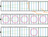 |
Fig. 3. Schematic illustration of the light cone construction, mixing ΛCDM and ΛLTB lens planes. The illustration shows the case of the smallest box, Box 1; see Table 2. See Sect. 3.4 for more details. |
4. Results
We now show the results of the simulations. Table 2 lists the LTB parameters that we adopt, together with a few summary statistics such as the total number of halos and the masses of the most massive halos. The cosmology is specified in Table 1. We adopt a grid in the LTB parameter space that covers inhomogeneities with radius rb from 200 Mpc h−1 to 1.6 Gpc h−1 and contrasts δ0 from ±0.1 to ±0.6, for a total of 68 models. The rationale behind this choice is to systematically explore the phenomenology of ΛLTB models in order to accurately understand how the growth of perturbations changes as a function of the LTB parameters.
It is worth mentioning that present-day observations rule out part of the models of Table 2. As discussed in the introduction, structures at the last scattering surface or along the line of sight (see the light cone construction of Fig. 3) cannot have nonlinear contrasts. Considering that we use the contrast at the center, δ0, and that the average contrast, Δ(t0, rt), is lower than δ0 (see Fig. 1, second panel from the top), the models with |δ0|> 0.3 are ruled out. On the other hand, if the observer is at the center, the models with |δ0|≥0.3 and rb ≥ 400 Mpc h−1 are excluded, as discussed in Appendix A, where the latest constraints by Camarena et al. (2021) are shown. Despite these observational constraints, we nevertheless simulate the models with |δ0|≥0.3 in order to test different approximation schemes for the growth of perturbations and their limits, which is the subject of a forthcoming work. In other words, we simulate a larger than observationally allowed parameter space in order to obtain a better modeling of linear and nonlinear structures. In particular, the main effects caused by spatial gradients will be evident in the most nonlinear models, allowing us to disentangle the signal from the noise with just one N-body realization (one seed). In any case, we sample the observationally relevant parameter space with |δ0|≤0.3 more finely.
Before presenting the evolution of the ΛLTB large-scale structure we will discuss the validation of the ΛLTB background evolution. The validation of the ΛCDM simulations is discussed in Appendix C, where we show that this first set of BEHOMO simulations have power spectrum and halo mass function accurate at the 5% level. As said before, the ΛLTB and ΛCDM simulations are paired so that numerical errors should approximately factor out when considering suitable ratios of relevant quantities.
4.1. Validation of the ΛLTB background dynamics
We validate the large-scale dynamics produced by the inhomogeneous (Newtonian) N-body simulations via the exact ΛLTB solution of general relativity described in Sect. 2. As we are not interested in small-scale dynamics, here we adopt lower-resolution simulations. Specifically, we consider the smallest box, Box 1, with 2563 particles and the largest box, Box 6, with 10243 particles, both with the largest contrasts of δ0 = ±0.6. Box 1 has a side of 500 Mpc h−1 and inhomogeneity radius of rb = 200 Mpc h−1, while Box 6 has side of 4000 Mpc h−1 and rb = 1600 Mpc h−1 (see Table 2). In order to precisely test the background dynamics, we simulate an inhomogeneous universe without the standard primordial Gaussian perturbations, that is, we adopt a very small amplitude of the primordial power spectrum, As ≈ 0.
Figure 4 compares the density and velocity profiles at z = 0. Using Eq. (38), we connect the longitudinal velocities, v∥, from the simulation to the perpendicular Hubble rate, H⊥:
![Mathematical equation: $$ \begin{aligned} { v}_{\parallel }(t,\chi ) = a(t) \, \chi \, \big [ H_{\perp }(t,r) - H(t) \big ] \,. \end{aligned} $$](/articles/aa/full_html/2022/08/aa43539-22/aa43539-22-eq90.gif) (68)
(68)
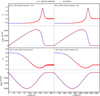 |
Fig. 4. Density and velocity profiles at z = 0 for the smallest and largest boxes with the largest contrasts; see Table 2. In order to precisely test the background dynamics, we simulate an inhomogeneous universe without the standard primordial Gaussian perturbations (As ≈ 0). The inhomogeneous (Newtonian) N-body simulations perfectly follow the GR solution. Furthermore, thanks to the scale invariance, their rescaled evolution is the same. See Sect. 4.1 for more details. |
One can see that the N-body simulation produces a background evolution that perfectly follows the GR one, even for inhomogeneities whose size is comparable with the Hubble radius. This is ultimately due to the fact that the ΛLTB dynamics is scale invariant thanks to the symmetries of the LTB metric (see Sect. 2.10).
As the LTB inhomogeneity is comparable in size with the box (rb = 0.4 L), one could wonder if such a large inhomogeneity would self-interact via the periodic boundary conditions. The answer is no because the LTB metric is matched at a finite radius rather than asymptotically (see Alonso et al. 2010, for the latter case). Therefore, a particle outside the inhomogeneity, such as the LTB structure itself with respect to its mirror LTB image, would locally experience the FLRW background and, thanks to the shell theorem (valid because of spherical symmetry), the same gravitational force as if there were no mirror images. Figure 4 confirms this.
The profile that we adopted is smooth at the center so that no artifacts are introduced when using the particle mesh part of OpenGadget3, as instead observed by Alonso et al. (2010) when adopting a cuspy profile. Using particle mesh is especially convenient (computationally less expensive) at early times when the tree algorithm struggles to deliver an accurate computation of the gravitational force (Springel et al. 2021).
4.2. The large-scale structure in an inhomogeneous universe
In Figs. 5 and 6 we show, for Box 1 and Box 3, the large-scale structure of the ΛLTB model as compared with the corresponding one of the ΛCDM model. While the larger circle marks the boundary rb of the ΛLTB inhomogeneity, the smaller one marks the transition from the central underdensity or overdensity to the compensating surrounding overdense or underdense shell. Also shown is the velocity field.
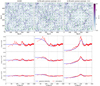 |
Fig. 5. Evolution of the large scale structure in the ΛLTB mode. The first row shows the large-scale structure of Box 1 at z = 0 of the overdense (middle panel) and underdense (right panel) ΛLTB models together with the corresponding ΛCDM model (left panel). The larger thin dashed circle marks the boundary, rb, of the ΛLTB inhomogeneity and the smaller one the radius, rt, at which δ(t0, rt) = 0, which marks the transition from the central underdensity or overdensity to the compensating overdense or underdense shell. The arrows show the velocity field. The density and velocity fields are obtained from the projection of the slice through the center, whose thickness is a fifth of the box side. One can see how the large-scale structure is identical outside the inhomogeneity, but it is distorted by the inhomogeneous bulk flow inside the LTB structure. The last three rows show the evolution of the radial profile, from z = 3.7 to z = 0 (Poissonian errors are negligible). Also shown is the GR solution given by the LTB solution of Sect. 2. The vertical lines mark rb and the smaller rt. While rb is fixed in comoving coordinates, rt moves because of the peculiar velocity of the LTB structure. |
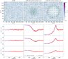 |
Fig. 6. As Fig. 5 but for Box 3. Because of the larger size, small-scale perturbations average out and the structure is more visible. |
Near the center one can see how matter structures are amplified or reduced when a central overdensity or underdensity is present, respectively. It is evident that the inhomogeneity causes a deformation of the positions and velocities of the corresponding particles in the ΛCDM simulation, and that such deformation disappears outside the inhomogeneity. In other words, the effect of the inhomogeneous background is to deform the large-scale structure of the ΛCDM model. Indeed, as pointed out earlier, the LTB perturbation is added on top of the primordial perturbations so that the structure of the cosmic web is preserved. Statistically, this will allow us to factor out cosmic variance when studying the effect of spatial gradients on observables.
The bottom panels of Figs. 5 and 6 show the evolution of the radial profiles at z = 0, 1.37 and 3.72 (from upper to lower panels). Also shown with the blue curves is the GR solution given by the LTB solution presented in Sect. 2. The vertical lines mark the inhomogeneity radius rb and the smaller transition radius rt. While rb is fixed in comoving coordinates, rt moves because of the peculiar velocity of the LTB structure. The LTB evolution of Box 1 and Box 3 is identical except for the scales involved, but the inhomogeneity is more clearly seen in Box 3 because, thanks to its larger size, small-scale perturbations average out.
5. Conclusions
In this paper we have presented the BEHOMO project and its first suite of simulations. The goal is to study, via the methods of numerical cosmology, the universe without assuming large-scale homogeneity and isotropy. In order to present a viable program, we considered early-FLRW cosmologies, which are models that, at early times, are near-FLRW such that the standard inflationary paradigm is maintained and the physics that leads to the CMB remains unchanged. As a first realization of these inhomogeneous cosmologies, we adopted the ΛLTB spherical model, on which the simulations presented here are based.
After a comprehensive review of the ΛLTB model, we described the numerical implementation of the ΛLTB simulations. The data products consist of 11 snapshots between redshifts z = 0 and z = 3.7 for each of the 68 simulations that have been performed, together with halo catalogs and lens planes relative to 21 snapshots, between redshift 0 and 4.2, for a total of approximately 180 TB of data. This is the first set of simulations of the ΛLTB model ever produced. In particular, we chose the inhomogeneity profile so that these simulations do not suffer from any spurious artifacts. Indeed, these Newtonian N-body simulations can perfectly reproduce the GR evolution even for deep Hubble-sized inhomogeneities.
With these data products, we plan to study in forthcoming papers the growth of perturbations at the linear and nonlinear level, gravitational lensing, cluster abundances and proprieties, and many other applications that we invite the scientific community to propose. Data can be obtained upon request.
After the exploitation of this first suite of simulations, the BEHOMO project will consider more realistic scenarios. One may consider exact solutions such as the quasi-spherical Szekeres model (Szekeres 1975), which features a dipole inhomogeneity instead of a spherical one (Bolejko 2007), or a more general inhomogeneous model to be solved via numerical GR codes. The ultimate goal is to constrain inhomogeneous models with present and future background and perturbation observables.
One can estimate the change in the expansion rate via linear perturbation theory. An adiabatic perturbation in density causes  , where f ≃ 0.5 is the present-day growth rate for the concordance ΛCDM model.
See Rigopoulos & Valkenburg (2012) for an alternative approach that uses a gradient series expansion.
Because of bulk motion, this is a conservative check.
github.com/TiagoBsCastro/SLICER (2021 version).
Acknowledgments
Warm thanks to Wessel Valkenburg for help during the early stages of this project and for sharing VoidDistances2020 and FalconIC. It is a pleasure to thank Klaus Dolag for sharing OpenGadget3, and Alessio Notari, Miguel Quartin and Emiliano Sefusatti for useful discussions. VM thanks CNPq (Brazil) and FAPES (Brazil) for partial financial support. This project has received funding from the European Union’s Horizon 2020 research and innovation programme under the Marie Skłodowska-Curie grant agreement No 888258 (https://cordis.europa.eu/project/id/888258). TC is supported by the fare Miur grant ‘ClustersXEuclid’ R165SBKTMA. TC and SB are supported by the INFN IN-DARK PD51 grant. DC thanks CAPES for financial support. AR acknowledges support from the grant PRIN-MIUR 2017 WSCC32. We acknowledge the use of the HOTCAT computing infrastructure of the Astronomical Observatory of Trieste of the National Institute for Astrophysics (INAF, Italy) (see Bertocco et al. 2020; Taffoni et al. 2020). We acknowledge the computing centre of Cineca and INAF, under the coordination of the “Accordo Quadro MoU per lo svolgimento di attivitá congiunta di ricerca Nuove frontiere in Astrofisica: HPC e Data Exploration di nuova generazione,” for the availability of computing resources and support. We acknowledge the use of the Santos Dumont supercomputer of the National Laboratory of Scientific Computing (LNCC, Brazil).
References
- Abate, A., Aldering, G., Allen, S. W., et al. 2012, ArXiv eprints [arXiv:1211.0310] [Google Scholar]
- Abbott, T. M. C., Aguena, M., Alarcon, A., et al. 2022, Phys. Rev. D, 105, 023520 [CrossRef] [Google Scholar]
- Abdalla, E., Abellán, G. F., Aboubrahim, A., et al. 2022, JHEAp, 34, 49 [NASA ADS] [Google Scholar]
- Adamek, J., Daverio, D., Durrer, R., & Kunz, M. 2016, JCAP, 07, 053 [CrossRef] [Google Scholar]
- Adamek, J., Clarkson, C., Daverio, D., Durrer, R., & Kunz, M. 2019, Class. Quant. Grav., 36, 014001 [NASA ADS] [CrossRef] [Google Scholar]
- Adamek, J., Barrera-Hinojosa, C., Bruni, M., et al. 2020, Class. Quant. Grav., 37, 154001 [NASA ADS] [CrossRef] [Google Scholar]
- Aghamousa, A., Aguilar, J., Ahlen, S., et al. 2016, ArXiv eprints [arXiv:1611.00036] [Google Scholar]
- Aghanim, N., Akrami, Y., Ashdown, M., et al. 2020, A&A, 641, A6; Erratum: 2021, 652, C4 [NASA ADS] [CrossRef] [EDP Sciences] [Google Scholar]
- Alfedeel, A. A. H., & Hellaby, C. 2010, Gen. Rel. Grav., 42, 1935 [NASA ADS] [CrossRef] [Google Scholar]
- Alonso, D., Garcia-Bellido, J., Haugbolle, T., & Vicente, J. 2010, Phys. Rev. D, 82, 123530 [NASA ADS] [CrossRef] [Google Scholar]
- Alonso, D., Garcia-Bellido, J., Haugboelle, T., & Knebe, A. 2012, Phys. Dark Univ., 1, 24 [NASA ADS] [CrossRef] [Google Scholar]
- Amendola, L., Appleby, S., Avgoustidis, A., et al. 2018, Liv. Rev. Rel., 21, 2 [Google Scholar]
- Angulo, R. E., Zennaro, M., Contreras, S., et al. 2021, MNRAS, 507, 5869 [NASA ADS] [CrossRef] [Google Scholar]
- Barrera-Hinojosa, C., & Li, B. 2020a, JCAP, 01, 007 [CrossRef] [Google Scholar]
- Barrera-Hinojosa, C., & Li, B. 2020b, JCAP, 04, 056 [CrossRef] [Google Scholar]
- Behroozi, P. S., Wechsler, R. H., & Wu, H.-Y. 2013, ApJ, 762, 109 [NASA ADS] [CrossRef] [Google Scholar]
- Bentivegna, E., & Bruni, M. 2016, Phys. Rev. Lett., 116, 251302 [NASA ADS] [CrossRef] [Google Scholar]
- Bertocco, S., Goz, D., Tornatore, L., et al. 2020, ASP Conf. Ser., 527, 303 [NASA ADS] [Google Scholar]
- Biswas, T., & Notari, A. 2008, JCAP, 06, 021 [CrossRef] [Google Scholar]
- Biswas, T., Mansouri, R., & Notari, A. 2007, JCAP, 12, 017 [CrossRef] [Google Scholar]
- Biswas, T., Notari, A., & Valkenburg, W. 2010, JCAP, 11, 030 [CrossRef] [Google Scholar]
- Blas, D., Lesgourgues, J., & Tram, T. 2011, JCAP, 1107, 034 [CrossRef] [Google Scholar]
- Bolejko, K. 2007, Phys. Rev. D, 75, 043508 [NASA ADS] [CrossRef] [Google Scholar]
- Bolejko, K., Celerier, M.-N., & Krasinski, A. 2011, Class. Quant. Grav., 28, 164002 [NASA ADS] [CrossRef] [Google Scholar]
- Bondi, H. 1947, MNRAS, 107, 410 [NASA ADS] [CrossRef] [Google Scholar]
- Bonoli, S., Marín-Franch, A., Varela, J., et al. 2021, A&A, 653, A31 [NASA ADS] [CrossRef] [EDP Sciences] [Google Scholar]
- Bonvin, C., Durrer, R., & Gasparini, M. A. 2006, Phys. Rev. D, 73, 023523; Erratum: 2012, 85, 029901 [NASA ADS] [CrossRef] [Google Scholar]
- Braun, R., Bourke, T., Green, J. A., Keane, E., & Wagg, J. 2015, PoS, AASKA14, 174 [Google Scholar]
- Bruni, M., Matarrese, S., & Pantano, O. 1995, ApJ, 445, 958 [NASA ADS] [CrossRef] [Google Scholar]
- Buchert, T., Carfora, M., Ellis, G. F. R., et al. 2015, Class. Quant. Grav., 32, 215021 [NASA ADS] [CrossRef] [Google Scholar]
- Bull, P., Clifton, T., & Ferreira, P. G. 2012, Phys. Rev. D, 85, 024002 [NASA ADS] [CrossRef] [Google Scholar]
- Cai, Y.-C., Cole, S., Jenkins, A., & Frenk, C. S. 2010, MNRAS, 407, 201 [NASA ADS] [CrossRef] [Google Scholar]
- Camarena, D., & Marra, V. 2018, Phys. Rev. D, 98, 023537 [NASA ADS] [CrossRef] [Google Scholar]
- Camarena, D., Marra, V., Sakr, Z., & Clarkson, C. 2021, MNRAS, 509, 1291 [NASA ADS] [CrossRef] [Google Scholar]
- Camarena, D., Marra, V., Sakr, Z., & Clarkson, C. 2022, Class. Quant. Grav., accepted [arXiv:2205.05422] [Google Scholar]
- Chung, D. J. H., & Romano, A. E. 2006, Phys. Rev. D, 74, 103507 [NASA ADS] [CrossRef] [Google Scholar]
- Clarkson, C. 2012, C.R. Phys., 13, 682 [NASA ADS] [CrossRef] [Google Scholar]
- Clarkson, C., & Regis, M. 2011, JCAP, 02, 013 [CrossRef] [Google Scholar]
- Clarkson, C., Clifton, T., & February, S. 2009, JCAP, 06, 025 [CrossRef] [Google Scholar]
- Clarkson, C., Ellis, G., Larena, J., & Umeh, O. 2011, Rept. Prog. Phys., 74, 112901 [NASA ADS] [CrossRef] [Google Scholar]
- Coles, P., & Lucchin, P. 2002, Cosmology: The Origin and Evolution of Cosmic Structure (Wiley) [Google Scholar]
- Dakin, J., Hannestad, S., & Tram, T. 2021, ArXiv eprints [arXiv:2112.01508] [Google Scholar]
- Daverio, D., Dirian, Y., & Mitsou, E. 2019, JCAP, 10, 065 [CrossRef] [Google Scholar]
- Dunsby, P., Goheer, N., Osano, B., & Uzan, J.-P. 2010, JCAP, 06, 017 [CrossRef] [Google Scholar]
- East, W. E., Wojtak, R., & Abel, T. 2018, Phys. Rev. D, 97, 043509 [NASA ADS] [CrossRef] [Google Scholar]
- Ellis, G. F. R. 1984, in Relativistic Cosmology: Its Nature, Aims and Problems, eds. B. Bertotti, F. de Felice, & A. Pascolini (Dordrecht, Netherlands: Springer), 215 [Google Scholar]
- Enqvist, K. 2008, Gen. Rel. Grav., 40, 451 [NASA ADS] [CrossRef] [Google Scholar]
- February, S., Larena, J., Clarkson, C., & Pollney, D. 2014, Class. Quant. Grav., 31, 175008 [CrossRef] [Google Scholar]
- Fidler, C., Tram, T., Rampf, C., et al. 2017, JCAP, 12, 022 [CrossRef] [Google Scholar]
- Flender, S., Hotchkiss, S., & Nadathur, S. 2013, JCAP, 02, 013 [CrossRef] [Google Scholar]
- Garcia-Bellido, J., & Haugboelle, T. 2008, JCAP, 09, 016 [CrossRef] [Google Scholar]
- Garcia-Bellido, J., & Haugboelle, T. 2009, JCAP, 0909, 028 [CrossRef] [Google Scholar]
- Giblin, J. T., Mertens, J. B., & Starkman, G. D. 2016, Phys. Rev. Lett., 116, 251301 [NASA ADS] [CrossRef] [Google Scholar]
- Giblin, J. T., Mertens, J. B., Starkman, G. D., & Tian, C. 2019, Phys. Rev. D, 99, 023527 [NASA ADS] [CrossRef] [Google Scholar]
- Green, S. R., & Wald, R. M. 2014, Class. Quant. Grav., 31, 234003 [NASA ADS] [CrossRef] [Google Scholar]
- Hui, L., & Greene, P. B. 2006, Phys. Rev. D, 73, 123526 [NASA ADS] [CrossRef] [Google Scholar]
- Kaiser, N. 2014, Elements of Astrophysics (CreateSpace Independent Publishing Platform) [Google Scholar]
- Kolb, E. W., Marra, V., & Matarrese, S. 2010, Gen. Rel. Grav., 42, 1399 [NASA ADS] [CrossRef] [Google Scholar]
- Laurent, P., Le Goff, J.-M., Burtin, E., et al. 2016, JCAP, 11, 060 [CrossRef] [Google Scholar]
- Lavinto, M., Räsänen, S., & Szybka, S. J. 2013, JCAP, 12, 051 [CrossRef] [Google Scholar]
- Leroy, M., Garrison, L., Eisenstein, D., Joyce, M., & Maleubre, S. 2021, MNRAS, 501, 5064 [NASA ADS] [CrossRef] [Google Scholar]
- Lim, W. C., Regis, M., & Clarkson, C. 2013, JCAP, 10, 010 [CrossRef] [Google Scholar]
- Macpherson, H. J., Price, D. J., & Lasky, P. D. 2019, Phys. Rev. D, 99, 063522 [NASA ADS] [CrossRef] [Google Scholar]
- Marra, V., & Notari, A. 2011, Class. Quant. Grav., 28, 164004 [NASA ADS] [CrossRef] [Google Scholar]
- Marra, V., & Paakkonen, M. 2012, JCAP, 1201, 025 [CrossRef] [Google Scholar]
- Marra, V., Kolb, E. W., Matarrese, S., & Riotto, A. 2007, Phys. Rev. D, 76, 123004 [NASA ADS] [CrossRef] [Google Scholar]
- Matarrese, S., Pantano, O., & Saez, D. 1993, Phys. Rev. D, 47, 1311 [NASA ADS] [CrossRef] [Google Scholar]
- Matarrese, S., Mollerach, S., & Bruni, M. 1998, Phys. Rev. D, 58, 043504 [NASA ADS] [CrossRef] [Google Scholar]
- Meyer, S., Redlich, M., & Bartelmann, M. 2015, JCAP, 03, 053 [CrossRef] [Google Scholar]
- Michaux, M., Hahn, O., Rampf, C., & Angulo, R. E. 2020, MNRAS, 500, 663 [NASA ADS] [CrossRef] [Google Scholar]
- Moss, A., Zibin, J. P., & Scott, D. 2011, Phys. Rev. D, 83, 103515 [NASA ADS] [CrossRef] [Google Scholar]
- Nadathur, S., Hotchkiss, S., & Sarkar, S. 2012, JCAP, 06, 042 [CrossRef] [Google Scholar]
- Nadathur, S., Lavinto, M., Hotchkiss, S., & Räsänen, S. 2014, Phys. Rev. D, 90, 103510 [NASA ADS] [CrossRef] [Google Scholar]
- Nishikawa, R., Yoo, C.-M., & Nakao, K.-I. 2012, Phys. Rev. D, 85, 103511 [NASA ADS] [CrossRef] [Google Scholar]
- Ntelis, P., Hamilton, J.-C., Le Goff, J.-M., et al. 2017, JCAP, 06, 019 [CrossRef] [Google Scholar]
- Perivolaropoulos, L., & Skara, F. 2022, New Astron. Rev., 95, 101659 [CrossRef] [Google Scholar]
- Perlmutter, S., Aldering, G., Goldhaber, G., et al. 1999, ApJ, 517, 565 [Google Scholar]
- Ragagnin, A., Dolag, K., Wagner, M., et al. 2020, in Parallel Computing: Technology Trends, ed. I. Foster, Adv. Parallel Comput., 36, 209 [Google Scholar]
- Rasanen, S. 2009, Phys. Rev. D, 79, 123522 [NASA ADS] [CrossRef] [Google Scholar]
- Redlich, M., Bolejko, K., Meyer, S., Lewis, G. F., & Bartelmann, M. 2014, A&A, 570, A63 [NASA ADS] [CrossRef] [EDP Sciences] [Google Scholar]
- Riess, A. G., Filippenko, A. V., Challis, P., et al. 1998, AJ, 116, 1009 [Google Scholar]
- Riess, A. G., Yuan, W., Macri, L. M., et al. 2021, ApJ, accepted [arXiv:2112.04510] [Google Scholar]
- Rigopoulos, G., & Valkenburg, W. 2012, Phys. Rev. D, 86, 043523 [NASA ADS] [CrossRef] [Google Scholar]
- Sachs, R. K., & Wolfe, A. M. 1967, ApJ, 147, 73 [NASA ADS] [CrossRef] [Google Scholar]
- Sakai, N., & Inoue, K. T. 2008, Phys. Rev. D, 78, 063510 [NASA ADS] [CrossRef] [Google Scholar]
- Scrimgeour, M., Davis, T., Blake, C., et al. 2012, MNRAS, 425, 116 [Google Scholar]
- Silk, J. 1977, A&A, 59, 53 [NASA ADS] [Google Scholar]
- Springel, V. 2005, MNRAS, 364, 1105 [Google Scholar]
- Springel, V., Pakmor, R., Zier, O., & Reinecke, M. 2021, MNRAS, 506, 2871 [NASA ADS] [CrossRef] [Google Scholar]
- Stebbins, A. 2012, Int. J. Mod. Phys. D, 21, 1242017 [NASA ADS] [CrossRef] [Google Scholar]
- Sussman, R. A. 2011, Class. Quant. Grav., 28, 235002 [NASA ADS] [CrossRef] [Google Scholar]
- Szekeres, P. 1975, Commun. Math. Phys., 41, 55 [NASA ADS] [CrossRef] [Google Scholar]
- Taffoni, G., Becciani, U., Garilli, B., et al. 2020, ASP Conf. Ser., 527, 307 [NASA ADS] [Google Scholar]
- Valkenburg, W. 2012a, JCAP, 01, 047 [CrossRef] [Google Scholar]
- Valkenburg, W. 2012b, Gen. Rel. Grav., 44, 2449 [NASA ADS] [CrossRef] [Google Scholar]
- Valkenburg, W., & Hu, B. 2015, JCAP, 09, 054 [CrossRef] [Google Scholar]
- Valkenburg, W., & Villaescusa-Navarro, F. 2017, MNRAS, 467, 4401 [NASA ADS] [CrossRef] [Google Scholar]
- Valkenburg, W., Marra, V., & Clarkson, C. 2014, MNRAS, 438, L6 [CrossRef] [Google Scholar]
- Van Acoleyen, K. 2008, JCAP, 10, 028 [CrossRef] [Google Scholar]
- Vielva, P. 2010, Adv. Astron., 2010 [NASA ADS] [CrossRef] [Google Scholar]
- Villaescusa-Navarro, F. 2018, Astrophysics Source Code Library [record ascl:1811.008] [Google Scholar]
- Wang, L.-M., & Steinhardt, P. J. 1998, ApJ, 508, 483 [NASA ADS] [CrossRef] [Google Scholar]
- Yamamoto, K., Marra, V., Mukhanov, V., & Sasaki, M. 2016, JCAP, 03, 030 [CrossRef] [Google Scholar]
- Zhang, P., & Stebbins, A. 2011, Phys. Rev. Lett., 107, 041301 [NASA ADS] [CrossRef] [Google Scholar]
- Zibin, J. P. 2008, Phys. Rev. D, 78, 043504 [NASA ADS] [CrossRef] [Google Scholar]
- Zibin, J. P. 2011, Phys. Rev. D, 84, 123508 [NASA ADS] [CrossRef] [Google Scholar]
- Zibin, J. P. 2021, ArXiv eprints [arXiv:1408.4442] [Google Scholar]
- Zibin, J. P., & Moss, A. 2011, Class. Quant. Grav., 28, 164005 [NASA ADS] [CrossRef] [Google Scholar]
Appendix A: Latest constraints on ΛLTB
Here, we show the latest constraints on the ΛLTB model for the case of the observer at the center of the spherical inhomogeneity, as obtained in Camarena et al. (2021). In Fig. A.1 we report the constraints using the same LTB parameters that are adopted here, that is, the central contrast δ0 and inhomogeneous size rb. We see that contrasts |δ0|≳0.2 are ruled out at scales rb ≳ 300 Mpc/h. We note, however, that Camarena et al. (2021) adopted a different curvature profile with respect to the one of Eq. (19).
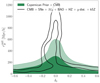 |
Fig. A.1. Marginalized constraints on the central contrast, δ0, and inhomogeneous size, rb, of the ΛLTB model at the 68% and 95% confidence level. The empty contours show the constraints from the CMB, BAOs, type Ia supernovae, the local H0, cosmic chronometers, Compton y-distortion, and the kSZ effect. The green area shows the region of the parameter space that is allowed by the standard model, here represented via the Copernican prior convolved with the CMB likelihood. See Camarena et al. (2021) for more details. |
Appendix B: OpenGadget3 performance
Figure B.1 illustrates how the execution of a simulation with OpenGadget3 is affected by the background inhomogeneity. We show the CPU times of the various internal algorithms, as a function of the scale factor, for the most nonlinear ΛLTB simulations (δ0 = −0.6, bottom) and the corresponding ΛCDM ones (top). One can see a very similar behavior, with a small increase in tree imbalance for the ΛLTB simulation.
 |
Fig. B.1. Logs of two ΛLTB simulations (bottom) and the corresponding ΛCDM ones (top) executed with OpenGadget3. |
For all simulations, the parameters that control the structure of the gravity solver are set to Asmth = 1.25 and Rcut = 4.5. Asmth sets the scale in units of mesh-cells that defines the long-range/short-range force-split in the TreePM algorithm. A larger value of Asmth will make the transition region better resolved by the mesh, yielding higher accuracy and less residual scatter in the force matching region, but at the same time the region that needs to be covered by the tree grows, which makes the computation more expensive. Rcut sets the maximum radius out to which the short-range tree-force is evaluated in case the TreePM algorithm is used.
We also tested the performance of the GPU porting of OpenGadget3 using OpenACC directives that was presented in Ragagnin et al. (2020). We found that the GPU porting is ≈40% faster when using 2563 particles and 2563 PM elements, but that the performance is similar when using 2563 particles and 5123 PM elements and that it is ≈20% slower when using 5123 particles and 10243 PM elements. From the log files one can see that the “pmgrav” module takes ≈30% resources up to z = 1.5 and ≈20% up to z = 0. Given these preliminary results, we used the version of OpenGadget3 without GPUs.
Appendix C: Validation of the ΛCDM simulations
Here, we validate the ΛCDM simulations against the Bias And Clustering Calculations Optimised (BACCO) emulator (v2.1.0, Angulo et al. 2021) and the halo mass function of Castrone et al. (in prep.). The emulator is expected to be accurate at the 2% level, and the Castro22 mass function strives to obtain a better than 1% calibration for next-generation surveys.
First, we consider the power spectrum. Figure C.1 compares the boost factor P(k, z)/P(k, z = 49) with the one from the BACCO emulator (top for z = 0, bottom for z = 1). We estimate the power spectrum with Pylians312 (Villaescusa-Navarro 2018) and consider wavenumbers till a tenth of the Nyquist wavenumber so that aliasing errors are negligible. Error bars are estimated via  where Nk is the number of independent modes used to estimate P(k), and nv is the number density in the simulation box. We see that all boxes but the smallest Box 1 have better than 5% accurate power spectrum. We adopted the same seed for all the simulations, and the first few modes happened to have less power with respect to the theoretical spectrum (see Fig. C.2). In the case of Box 1, the first few modes are at a larger wavenumber so that the worse accuracy that we see in this case could be due to mode coupling. Indeed, having less power on large scales in the initial conditions also implies that less power is transferred to smaller scales, due to the coupling between different modes during the nonlinear evolution. We note that the discrepancy is indeed less severe at z = 1 (Fig. C.1, bottom panel). We also performed a Box-2 simulation (1 Gpc and Npart = 10243; see Table 2) with the cosmology of Castrone et al. (in prep.) and compared it with a 1-Gpc simulation with Npart = 40643 that was run according to the specifications of Castrone et al. (in prep.). We found an agreement better than 5%.
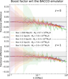 |
Fig. C.1. Boost factor P(k, z)/P(k, z = 49) as compared with the one from the BACCO emulator (top for z = 0, bottom for z = 1). |
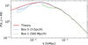 |
Fig. C.2. Initial measured power spectrum for Box 1 and Box 5. The first few modes have less power with respect to the theoretical spectrum (we adopted the same seed for all simulations). |
Next, we consider halo abundances. Figure C.3 compares the halo mass function against the one of Castrone et al. (in prep.), which adopts the virial spherical overdensity. We adopt Gaussian error bars from the corresponding Poisson distributions. The top panel shows the fractional difference for Box 1 and increasing mass resolution, that is, 2563, 5123, and 10243 particles. One sees that with a particle mass of ≲1011 M⊙/h one reaches a 5% accuracy. Then we show, in the bottom panel, the fractional difference for the other boxes, again reaching a 5% accuracy.
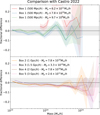 |
Fig. C.3. Halo mass function from the simulations against that of Castrone et al. (in prep.), which adopts the virial spherical overdensity. See Appendix C for more details. |
Concluding, the ΛCDM simulations of this first set of BEHOMO simulations have power spectrum and halo mass function accurate at the 5% level (except Box 1). We note that the ΛLTB and ΛCDM simulations are paired so that numerical errors should approximately factor out when considering suitable ratios of relevant quantities.
All Tables
Snapshots that were saved during the runs for the generation of the halo catalog and lens planes.
All Figures
|
Fig. 1. LTB quantities as a function of the FLRW comoving coordinate, χ, at the present time, t0. The two dotted lines mark the positions of the shells relative to rt and rb. See Sect. 2.7. |
| In the text | |
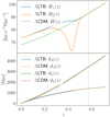 |
Fig. 2. LTB quantities as a function of redshift. See Sect. 2.7. |
| In the text | |
|
Fig. 3. Schematic illustration of the light cone construction, mixing ΛCDM and ΛLTB lens planes. The illustration shows the case of the smallest box, Box 1; see Table 2. See Sect. 3.4 for more details. |
| In the text | |
|
Fig. 4. Density and velocity profiles at z = 0 for the smallest and largest boxes with the largest contrasts; see Table 2. In order to precisely test the background dynamics, we simulate an inhomogeneous universe without the standard primordial Gaussian perturbations (As ≈ 0). The inhomogeneous (Newtonian) N-body simulations perfectly follow the GR solution. Furthermore, thanks to the scale invariance, their rescaled evolution is the same. See Sect. 4.1 for more details. |
| In the text | |
|
Fig. 5. Evolution of the large scale structure in the ΛLTB mode. The first row shows the large-scale structure of Box 1 at z = 0 of the overdense (middle panel) and underdense (right panel) ΛLTB models together with the corresponding ΛCDM model (left panel). The larger thin dashed circle marks the boundary, rb, of the ΛLTB inhomogeneity and the smaller one the radius, rt, at which δ(t0, rt) = 0, which marks the transition from the central underdensity or overdensity to the compensating overdense or underdense shell. The arrows show the velocity field. The density and velocity fields are obtained from the projection of the slice through the center, whose thickness is a fifth of the box side. One can see how the large-scale structure is identical outside the inhomogeneity, but it is distorted by the inhomogeneous bulk flow inside the LTB structure. The last three rows show the evolution of the radial profile, from z = 3.7 to z = 0 (Poissonian errors are negligible). Also shown is the GR solution given by the LTB solution of Sect. 2. The vertical lines mark rb and the smaller rt. While rb is fixed in comoving coordinates, rt moves because of the peculiar velocity of the LTB structure. |
| In the text | |
|
Fig. 6. As Fig. 5 but for Box 3. Because of the larger size, small-scale perturbations average out and the structure is more visible. |
| In the text | |
|
Fig. A.1. Marginalized constraints on the central contrast, δ0, and inhomogeneous size, rb, of the ΛLTB model at the 68% and 95% confidence level. The empty contours show the constraints from the CMB, BAOs, type Ia supernovae, the local H0, cosmic chronometers, Compton y-distortion, and the kSZ effect. The green area shows the region of the parameter space that is allowed by the standard model, here represented via the Copernican prior convolved with the CMB likelihood. See Camarena et al. (2021) for more details. |
| In the text | |
|
Fig. B.1. Logs of two ΛLTB simulations (bottom) and the corresponding ΛCDM ones (top) executed with OpenGadget3. |
| In the text | |
|
Fig. C.1. Boost factor P(k, z)/P(k, z = 49) as compared with the one from the BACCO emulator (top for z = 0, bottom for z = 1). |
| In the text | |
|
Fig. C.2. Initial measured power spectrum for Box 1 and Box 5. The first few modes have less power with respect to the theoretical spectrum (we adopted the same seed for all simulations). |
| In the text | |
|
Fig. C.3. Halo mass function from the simulations against that of Castrone et al. (in prep.), which adopts the virial spherical overdensity. See Appendix C for more details. |
| In the text | |
Current usage metrics show cumulative count of Article Views (full-text article views including HTML views, PDF and ePub downloads, according to the available data) and Abstracts Views on Vision4Press platform.
Data correspond to usage on the plateform after 2015. The current usage metrics is available 48-96 hours after online publication and is updated daily on week days.
Initial download of the metrics may take a while.