© The Authors 2023

1. Introduction

Modern cosmology relies on several fundamental assumptions, such as the hypothesis that we do not occupy a special location in the Universe. Thanks to this assumption, called the Copernican principle, cosmologists have made tremendous advances in the understanding of the Universe and laid the foundation of the standard cosmological model. The Copernican principle, along with the fact that the Universe appears to be statistically isotropic, implies that our Universe is homogeneous and isotropic on sufficiently large scales, eliminating any possible spatial dependence in the cosmological parameters. Equivalently, the space-time is accurately described by the Friedmann-Lemaître-Robertson-Walker (FLRW) metric. Clearly, any violation of the Copernican principle indicates a breakdown of the FLRW paradigm and, therefore, of the standard cosmological model. Thus, testing the Copernican principle is an essential task in cosmology.

One of the most fundamental tests of the Copernican principle comes from observations of our motion with respect to the cosmic microwave background (CMB) rest frame, which induces a kinematic dipole that has already been observed in the CMB (Planck Collaboration XXVII 2014; Planck Collaboration Int. LVI 2020; Ferreira & Quartin 2021; Saha et al. 2021), the local bulk flow (Colin et al. 2011; Feindt et al. 2013; Hudson et al. 2004; Carrick et al. 2015), X-ray clusters (Migkas et al. 2020, 2021), type Ia supernovae (SNe; Mohayaee et al. 2021; Rahman et al. 2022), high redshift radio sources (Colin et al. 2017; Bengaly et al. 2018; Siewert et al. 2021), and distant quasars (Secrest et al. 2021)¹. Many of these observations have intrinsic systematic errors that have to be taken into account (Dalang & Bonvin 2022) in order to avoid theoretical biases. Another route is to perform null tests of the FLRW metric (see Nesseris et al. 2022, for recent forecasts) or to estimate the homogeneity scale (Yadav et al. 2010; Kim et al. 2022).

Additionally, it is also possible to test the Copernican principle by assuming an inhomogeneous metric, such as that of the Lemaître-Tolman-Bondi (LTB) model (Garcia-Bellido & Haugboelle 2008a; February et al. 2010; Valkenburg et al. 2014; Redlich et al. 2014). In fact, current observations can meaningfully test the Copernican principle, leading to constraints on deviations from the FLRW metric at almost the cosmic variance level (Camarena et al. 2021).

In this paper we explore the precision with which next-generation surveys will probe for violations of the Copernican principle. Specifically, we focus on Euclid (Laureijs et al. 2011), which is an M-class space mission of the European Space Agency planned to be launched in 2023. The satellite will carry two instruments on board – the visible imager (VIS; Cropper et al. 2018) and the near-infrared spectrophotometric instrument (Prieto et al. 2012; Maciaszek et al. 2016) – which will carry out a photometric and spectroscopic galaxy survey covering over 15 000 deg² of the sky, with the aim of measuring the growth of the large-scale structure (LSS) up to a redshift of z ∼ 2 (Euclid Collaboration 2022).

Euclid will have two main, complementary cosmological probes, namely galaxy clustering and weak lensing from the photometric survey and galaxy clustering from the spectroscopic survey. While photometric surveys image a larger number of galaxies than spectroscopic ones, they also have larger redshift uncertainties. On the other hand, spectroscopic galaxy surveys have much higher radial precision, but target many fewer objects. Euclid has very high spectroscopic accuracy; it will be able to make very precise measurements of galaxy clustering that also include the radial dimension, that is to say, it will be able to probe clustering along the line of sight. In this work we create mock baryon acoustic oscillation (BAO) data, in accordance with Euclid’s spectroscopic survey specifications, based on the Fisher matrix approach of Euclid Collaboration (2020a, hereafter EC20).

Furthermore, we also stress some of the possible synergies between Euclid and other contemporary surveys. The latter include the Legacy Survey of Space and Time (LSST) performed at the Vera C. Rubin Observatory (LSST Science Collaboration 2009) and that of the Dark Energy Spectroscopic Instrument (DESI; DESI Collaboration 2016) since they will be complementary to Euclid in terms of redshift, thus significantly extending the possible redshift range of our analysis.

Finally, forecast constraints on deviations from the Copernican principle were presented in Amendola et al. (2018), where a joint analysis between Euclid (Laureijs et al. 2011) and a stage IV SN mission (Albrecht et al. 2006, assuming SNAP as a concrete example) was performed. Here we update the constraints of this analysis by using more recent Euclid specifications (see EC20) while also considering synergies with other surveys.

This paper is organised as follows: In Sect. 2 we briefly review the dynamics of a spherically inhomogeneous space-time based on the LTB metric but with the addition of a cosmological constant, Λ (i.e. the ΛLTB model) and discuss our particular choices for its arbitrary functions. In Sect. 3 we present the data used in our analysis and explain how mock catalogues are produced considering particular fiducial cosmologies, while in Sect. 4 we define and discuss the Copernican prior. Our results are presented and discussed in Sects. 5 and 6. We conclude in Sect. 7.

2. Spherically symmetric inhomogeneous models with a cosmological constant

A spherically inhomogeneous space-time can be modelled using the ΛLTB model, which practically is a standard cosmological constant Λ and cold dark matter (CDM) model endowed with a spherical inhomogeneity. Here, we aim to test the homogeneity of the Universe, and thus, we neglect anisotropic degrees of freedom by placing the observer at the centre of the spherical inhomogeneity. In this section we briefly review the ΛLTB model presented in Camarena et al. (2021)²; a comprehensive review is given in Marra et al. (2022).

Hereafter, we use a prime to denote a partial derivative with respect to the radial coordinate, r, while we use a dot to denote a partial derivative with respect to the time coordinate, t.

2.1. Dynamics

The LTB metric can be written as

$$\begin{array}{c}\hfill \mathrm{d}{s}^2=-c^2\mathrm{d}{t}^2+\frac{R^{\prime 2}(t,r)}{1-K(r)r^2}\mathrm{d}{r}^2+R^2(r,t)(\mathrm{d}{\theta }^2+{sin}^2\theta \mathrm{d}{\varphi }^2),\end{array}$$(1)

where the curvature K(r) is an arbitrary function of the radial coordinate. The FLRW metric can be recovered by imposing K = constant and R = a(t) r, with a(t) as the FLRW scale factor. From the line element Eq. (1), we can define the transverse and longitudinal scale factors, a_⊥ = R(r, t)/r and a_∥ = R′(r, t), respectively. The two scale factors define two different expansion rates given by

$$\begin{array}{c}\hfill H_{\perp }(t,r)\equiv \frac{{\dot{a}}_{\perp }}{a_{\perp }},H_{\Vert }(t,r)\equiv \frac{{\dot{a}}_{\Vert }}{a_{\Vert }}·\end{array}$$(2)

Solving Einstein’s equations with a cosmological constant, we obtain an equation analogue to the first Friedmann equation,

$$\begin{array}{c}\hfill \frac{H_{\perp }^2}{H_{\perp 0}^2}={\mathrm{\Omega }}_{\mathrm{m},0}{\left(\frac{a_{\perp 0}}{a_{\perp }}\right)}^3+{\mathrm{\Omega }}_{k,0}{\left(\frac{a_{\perp 0}}{a_{\perp }}\right)}^2+{\mathrm{\Omega }}_{\mathrm{\Lambda },0},\end{array}$$(3)

where the present-day density parameters are now functions of r,

$$\begin{array}{cc}& {\mathrm{\Omega }}_{\mathrm{\Lambda },0}(r)=\frac{\mathrm{\Lambda }{c}^2}{3H_{\perp 0}^2},\hfill \end{array}$$(4)

$$\begin{array}{cc}& {\mathrm{\Omega }}_{k,0}(r)=-\frac{K(r)c^2}{H_{\perp 0}^2{a}_{\perp 0}^2},\hfill \end{array}$$(5)

$$\begin{array}{cc}& {\mathrm{\Omega }}_{\mathrm{m},0}(r)=\frac{2m(r)}{H_{\perp 0}^2{a}_{\perp 0}^3{r}^3},\hfill \end{array}$$(6)

which satisfy Ω_m, 0(r)+Ω_k, 0(r)+Ω_Λ, 0(r) = 1. It should be noted that we have defined H_⊥0 ≡ H_⊥(t₀, r) and a_⊥0 ≡ a_⊥(t₀, r).

From Eq. (6) we can see that Einstein’s equations introduce another arbitrary function: the Euclidean mass m(r). This function arises as a constant of integration and is defined via

$$\begin{array}{c}\hfill m(r)={\displaystyle {\int }_0^r\mathrm{d}r\prime 4\pi G{\rho }_{\mathrm{m}}(t,r\prime )a_{\Vert }{a}_{\perp }^2{r}^{\prime 2},}\end{array}$$(7)

where ρ_m(t, r) is the local matter density.

Another arbitrary function of the ΛLTB model is the Big Bang function, t_BB(r). This can be interpreted as the time corresponding to the Big Bang singularity surface, and it emerges from integration of Eq. (3):

$$\begin{array}{c}\hfill t-t_{\mathrm{BB}}(r)=\frac{1}{H_{\perp 0}(r)}{\displaystyle {\int }_0^{\chi }\frac{\mathrm{d}x}{\sqrt{{\mathrm{\Omega }}_{\mathrm{m},0}(r)x^{-1}+{\mathrm{\Omega }}_{k,0}(r)+{\mathrm{\Omega }}_{\mathrm{\Lambda },0}(r)x^2}},}\end{array}$$(8)

where χ = a_⊥(t, r)/a_⊥0. We note that the last integral defines the age of the Universe, t₀, when integrated from zero to one.

Finally, from the line element Eq. (1) it follows that the geodesic equations are

$$\begin{array}{c}\hfill \frac{\mathrm{d}t}{\mathrm{d}z}=-\frac{1}{(1+z)H_{\Vert }(t,r)},\frac{\mathrm{d}r}{\mathrm{d}z}=-\frac{c\sqrt{1-K(r)r^2}}{(1+z)a_{\Vert }(t,r)H_{\Vert }(t,r)}·\end{array}$$(9)

2.2. Free functions

As shown above, the ΛLTB model has three arbitrary functions: K(r), m(r), and t_BB(r). One of these functions is just a gauge freedom that can be fixed by re-scaling the radial coordinate. Here, we fix the radial coordinate r such that the mass function satisfies m(r)∝r³; we will later present the missing normalisation of the Euclidean mass. On the other hand, a Big Bang function different from zero introduces decaying modes into the matter density (Silk 1977). The presence of these modes leads to a disagreement with the standard scenario of inflation (Zibin 2008). Thus, to ensure the absence of decaying modes on the matter density we set t_BB(r) = 0, which also implies that the Big Bang singularity happens everywhere simultaneously.

Hence, we end up with just one arbitrary function, the curvature profile K(r). Here, we adopt the monotonic compensated profile given by

$$\begin{array}{c}\hfill K(r)=K_{\mathrm{B}}+(K_{\mathrm{C}}-K_{\mathrm{B}})P_3(r/r_{\mathrm{B}}),\end{array}$$(10)

where r_B is the comoving radius of the spherical inhomogeneity, K_B is the background curvature, K_C is the central curvature, and the function P₃ follows,

$$\begin{array}{c}\hfill P_3(x)=\{\begin{array}{cc}1-exp[-{(1-x)}^3/x]\hfill & \mathrm{for}0\le x<1\hfill \\ 0\hfill & \mathrm{for}1\le x\hfill \end{array},\end{array}$$(11)

with x = r/r_B. Thus, Eq. (10) ensures a smooth transition between the LTB and FLRW metrics; the ΛLTB model asymptotes to the ΛCDM model at scales r ≥ r_B.

We note that while we have fixed m(r) and t_BB(r) using physical arguments, our choice of K(r) remains arbitrary and could have a significant impact on our analysis. In Appendix A we discuss our choice and compare it with another ΛLTB model. We also present an extra analysis performed using an extension of Eq. (10). This further analysis shows that a more generalised curvature profile could weaken the constraints by up to a factor of ∼2.

Once the three arbitrary functions are fixed, we can compute ρ_m(r, t) in order to determine the matter density contrast using

$$\begin{array}{c}\hfill \delta (r,t):=\frac{{\rho }_{\mathrm{m}}(r,t)}{{\rho }_{\mathrm{m}}(r_{\mathrm{B}},t)}-1,\end{array}$$(12)

and we can also compute the mass (integrated) density contrast via

$$\begin{array}{cc}\hfill \mathrm{\Delta }(r,t_0)& =\frac{4\pi {\int }_0^r\mathrm{d}\overline{r}\delta (\overline{r},t_0)a_{\perp }^2(\overline{r},t_0)a_{\Vert }(\overline{r},t_0)r^2}{4\pi a_{\perp }^3(r,t_0)r^3/3}\hfill \\ \hfill & =\frac{m(r)}{4\pi G{R}^3(r,t_0)/3{\rho }_{\mathrm{m}}^{\mathrm{out}}(t_0)}-1=\frac{{\mathrm{\Omega }}_{\mathrm{m},0}(r)}{{\mathrm{\Omega }}_{\mathrm{m},0}^{\mathrm{out}}}{\left[\frac{H_{\perp 0}(r)}{H_{\perp 0}^{\mathrm{out}}}\right]}^2-1.\hfill \end{array}$$(13)

Here we use the superscript ‘out’ to denote the FLRW background quantities outside the inhomogeneity, for example ${\rho }_{\mathrm{m}}(r_{\mathrm{B}},t_0)={\rho }_{\mathrm{m}}^{\mathrm{out}}(t_0)$. We additionally make use of the FLRW comoving coordinate at the present time, which is defined as

$$\begin{array}{c}\hfill r^{\mathrm{out}}:=r{a}_{\perp 0}(r)/a^{\mathrm{out}}(t_0).\end{array}$$(14)

The top panel in Fig. 1 shows the matter and integrated mass density contrast as a function of r^out at t = t₀ for a deep and gigaparsec-scale void. Also displayed in the figure are ${\mathrm{\Omega }}_{\mathrm{m},0}(r^{\mathrm{out}})-{\mathrm{\Omega }}_{\mathrm{m},0}^{\mathrm{out}}$ and ${\mathrm{\Omega }}_{k,0}(r^{\mathrm{out}})-{\mathrm{\Omega }}_{k,0}^{\mathrm{out}}$, giving the deviations of the matter and curvature densities with respect to their ΛCDM counterparts (middle panel), along with the deviations of the transverse and longitudinal expansion rates with respect to $H_0^{\text{out}}$ (bottom panel).

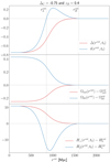Fig. 1. Several ΛLTB quantities as a function of the FLRW comoving coordinate rout. Top: density contrast of matter, δ(r) = ρm(r, t0)/ρm(rB, t0)−1, and integrated mass, Δ(r), as functions of the FLRW comoving coordinate. At radius $r_{\mathrm{L}}^{\mathrm{out}}$ the central structure ends and the compensating shell begins, while $r_{\mathrm{B}}^{\mathrm{out}}$ is the boundary of the spherical inhomogeneity. Middle: deviations from the background density of matter, ${\mathrm{\Omega }}_{\mathrm{m},0}^{\mathrm{out}}$, and curvature, ${\mathrm{\Omega }}_{k,0}^{\mathrm{out}}$, as a function of the FLRW comoving coordinate due to the radial dependence on Ωm, 0(r) and Ωk, 0(r). We note that the FLRW background quantities are recovered for $r\ge r_{\mathrm{B}}^{\mathrm{out}}$. Bottom: transverse and longitudinal fluctuations in the expansion rates as a function of the FLRW comoving coordinate.

It is important to highlight that the assumption of the profile Eq. (10) implicitly introduces a compensating scale, here denoted by $r_{\mathrm{L}}^{\mathrm{out}}[\delta (r_{\mathrm{L}}^{\mathrm{out}},t)=0]$, at which the central overdense or underdense region makes a transition to the surrounding mass-compensating underdense or overdense region. The $r_{\mathrm{L}}^{\mathrm{out}}$ and the $r_{\mathrm{B}}^{\mathrm{out}}$ scales are represented in Fig. 1 by the dotted vertical lines. Furthermore, one can note that at the centre of the inhomogeneity Δ(0, t) = δ(0, t), while at the boundary shell we have Δ(r_B, t) = δ(r_B, t) = 0. Since the LTB and FLRW metrics perfectly match at the boundary shell, then we have that $r_{\mathrm{B}}^{\mathrm{out}}=r_{\mathrm{B}}$. Finally, from Eq. (6) is possible to determine the missing normalisation of the Euclidean mass; specifically we find $m(r)={\mathrm{\Omega }}_{\mathrm{m},0}^{\mathrm{out}}{(H_0^{\mathrm{out}})}^2{r}^3/2$, while Eq. (5) leads to $K_{\mathrm{B}}=-{\mathrm{\Omega }}_{k,0}^{\mathrm{out}}{(H_0^{\mathrm{out}})}^2$.

2.3. Parameter space

We used the monteLLTB code to solve the dynamical equations and then to sample the parameter space of the ΛLTB model³. The monteLLTB code combines montepython (Audren et al. 2013; Brinckmann & Lesgourgues 2019) for the Markov chain Monte Carlo parameter space exploration and likelihoods, class (Blas et al. 2011) for the CMB computation and voiddistances2020 (Valkenburg 2012) for the ΛLTB metric functions via a wrapper that translates the montepython trial vector into an effective FLRW vector that is suitable for class (see Camarena et al. 2021 for details).

Since the LTB metric asymptotes to FLRW at r ≥ r_B, the background expansion of our model is specified by the standard six ΛCDM parameters: the normalised Hubble constant h := H₀/100, the baryon density Ω_b, 0, the cold dark matter density Ω_cdm, 0, the optical depth τ, the amplitude of the power spectrum A_s and its tilt n_s.

On the other hand, the spherically inhomogeneous region is fixed by the boundary redshift, z_B, and the mass density contrast at the centre of the inhomogeneity, Δ_C ≡ Δ(0, t). The parameters z_B and Δ_C are related to the parameters r_B and K_C, which explicitly appear in the definition of the curvature profile. As discussed in Sect. 4, we conveniently present our results using the compensating scale $r_{\mathrm{L}}^{\mathrm{out}}$ and the mass contrast at such a scale, Δ_L ≡ Δ(r_L, t₀).

We note that for Δ_C ≈ 0, the parameter space is highly degenerate so that the model could feature arbitrarily large values of z_B and be still allowed by the data. In order to overcome this issue, we adopt, as in Camarena et al. (2021), the flat prior z_B ∈ [0, 0.5]. This prior allows us to map non-Copernican structures of up to $r_{\mathrm{L}}^{\mathrm{out}}\sim 1$ Gpc.

3. Data

Here we present both the forecast and current data used to constrain the ΛLTB model. Although our goal is to forecast constraints on the Copernican principle given the forthcoming surveys, the inclusion of current data is needed to tightly constrain the ΛLTB parameter space at small scales.

Forecasted datasets are generated considering four fiducial models, which are based on the ΛCDM and ΛLTB models (see Table 1). By considering the ΛCDM forecast data we aim to determine the precision with which next-generation surveys will be able to probe for deviations from the FLRW metric. Meanwhile, by considering the inhomogeneous ΛLTB fiducial model, we aim to investigate the ability of future surveys to detect a violation of the Copernican principle. In order to assume a consistent fiducial model, current data have been re-scaled to agree with the aforementioned fiducial models. Such a re-scaling is performed following the procedure described in Appendix B. Furthermore, we also assume that there are no tensions among the different datasets; this includes tensions between early and late determinations. The theoretical predictions for the observables implemented here follow the equations discussed in Sect. 3 of Camarena et al. (2021). We note that, in order to fully calibrate the SN distances, we also assume a fiducial value for the absolute magnitude of SN data, that is, M₀ = −19.3.

3.1. Forecast data

In order to forecast how Euclid and other forthcoming surveys will constrain deviations from the Copernican principle, we created mock SN and BAO data; the former provide information on the luminosity distance, while the latter concern the Hubble parameter and the angular diameter distance. In particular, the recipes described here were used for the ΛCDM catalogues, while the ΛLTB catalogues are obtained by suitably re-scaling the former (see Appendix B).

The four fiducial cosmologies based on the ΛCDM and the ΛLTB model that we consider here are shown in Table 1; the former was also used in EC20. To make the mocks for the ΛCDM model, we calculated the redshift evolution of the Hubble parameter, along with the luminosity and angular diameter distances, using the recipe described in the next section, which is based on the specifications of Euclid and other LSS surveys. On the other hand, as mentioned before, the ΛLTB mock catalogues are obtained following the process described in Appendix B. Since computing correlation matrices for models far from the ΛCDM model is currently not possible (Harnois-Deraps et al. 2019; Friedrich et al. 2021; Ferreira & Marra 2022), we first compute the correlation matrix assuming the ΛCDM model. Then, we apply the method described in Appendix B to obtain the corresponding ΛLTB matrices.

Since future surveys like Euclid are expected to provide observations with high precision, it is important to be convinced that our analysis methods will be robust. Hence, in order to understand and take possible observational systematic uncertainties that can affect the measurements into account, several analyses, such as that of Euclid Collaboration (2020b), have been performed. In the latter, the observational systematic effects of the Euclid VIS instrument were studied, taking the modelling of the point spread function and the charge transfer inefficiency into account. Since these systematic effects are expected to be better understood by the time the data arrive, in this analysis we assume that they will be under control in the final data products. In any case, in what follows we in fact include several astrophysical systematic effects, such as the galaxy bias, as discussed in what follows.

3.1.1. SN surveys

In our analysis we focus on two forthcoming SN surveys, the first of which is based on the proposed Euclid DESIRE survey (Laureijs et al. 2011; Astier et al. 2014), while the second one is based on the specifications of the LSST. In particular, we assume that the Euclid DESIRE survey will observe 1700 SNe in the redshift range z ∈ [0.7, 1.6], while the one from the LSST survey will observe 8800 SNe in the redshift range z ∈ [0.1, 1.0], thus resulting in a total of 10 500 points.

In either case we consider the redshift distributions of the SN events as described in Astier et al. (2014), assuming the points are not correlated with each other. Even though the Euclid SN survey is not currently guaranteed to take place, we decided to include it in order to extend the redshift range of LSST at high z. For the SN mocks we include an observational error of the form ${\sigma }_{\text{tot},i}^2=\delta {\mu }_i^2+{\sigma }_{\text{flux}}^2+{\sigma }_{\text{scat}}^2+{\sigma }_{\text{intr}}^2$, where the terms corresponding to the intrinsic contributions, the scatter and the flux are the same for all events: σ_intr = 0.12, σ_scat = 0.025, and σ_flux = 0.01, respectively. Finally, we also include an error on the distance modulus μ = m − M₀ that scales linearly with z as δμ = e_M z, where e_M follows a Gaussian distribution with zero mean and standard deviation σ(e_M) = 0.01 (see Gong et al. 2010; Astier et al. 2014), which includes the possible redshift evolution of SNe not taken into account by the distance estimator (see Astier et al. 2014). However, while a value of e_M = 0.01 is required to take a possible systematic evolution into account, this would be added quadratically to an effective term of e_M = 0.055 arising from SN lensing. The latter has been theoretically calculated by several authors to be of the order of σ_lens ≃ 0.055 z, for example σ_lens = 0.052 z (Marra et al. 2013; Quartin et al. 2014), and σ_lens = 0.056 z (Ben-Dayan et al. 2013), while observationally it was determined, via the Supernova Legacy Survey to be σ_lens = (0.055 ± 0.04) z (Jonsson et al. 2010) and σ_lens = (0.054 ± 0.024) z (Kronborg et al. 2010).

3.1.2. Local prior on the Hubble constant

We also forecast a 1% measurement of the Hubble constant, which is the grand goal of the SH0ES collaboration,

$$\begin{array}{cc}\hfill H_0& =\{\begin{array}{cc}67.00\pm 0.67\mathrm{km}{\mathrm{s}}^{-1}{\mathrm{Mpc}}^{-1}\hfill & \mathrm{for}\mathrm{\Lambda }\mathrm{CDM}\hfill \\ 67.62\pm 0.68\mathrm{km}{\mathrm{s}}^{-1}{\mathrm{Mpc}}^{-1}\hfill & \mathrm{for}\mathrm{\Lambda }\mathrm{LTB}1\hfill \\ 68.22\pm 0.68\mathrm{km}{\mathrm{s}}^{-1}{\mathrm{Mpc}}^{-1}\hfill & \mathrm{for}\mathrm{\Lambda }\mathrm{LTB}2\hfill \\ 68.45\pm 0.68\mathrm{km}{\mathrm{s}}^{-1}{\mathrm{Mpc}}^{-1}\hfill & \mathrm{for}\mathrm{\Lambda }\mathrm{LTB}3\hfill \end{array},\hfill \end{array}$$(15)

where the central value is given by the fiducial H₀ value for the ΛCDM fiducial model, meanwhile for the ΛLTB models this central value is the expected value given the methodology described in Appendix C. Here, as mentioned earlier, we consider a scenario in which there is no tension between early and late determinations of the Hubble constant. By assuming a single consistent fiducial model, we focus on the constraining potential of future surveys to test the Copernican principle, leaving the issue of the Hubble tension to other studies. This is in part justified since Camarena et al. (2021, 2022) shown that a large inhomogeneity cannot explain away the Hubble tension. Finally, we impose the Gaussian prior of Eq. (15) on $H_0^{\text{L}}$; the corresponding Hubble constant value for an inhomogeneous model (see Appendix C for a detailed discussion).

3.1.3. Large-scale structure surveys

Here, we now briefly describe our procedure for creating mock BAO data based on the specifications of Euclid via a Fisher matrix approach, following the methodology of EC20 for the spectroscopic survey, on which we focus since we are interested in obtaining precise measurements of the angular diameter distance D_A(z) and the Hubble parameter H(z). We do not consider weak lensing by Euclid, nor other perturbation level observables such as redshift space distortions, because there is not yet a fully developed linear perturbation theory on inhomogeneous backgrounds such as the LTB⁴. A discussion and the numerical simulation of the LSS on an LTB background is provided in Marra et al. (2022) and references therein.

As was extensively discussed in EC20, the main targets of the Euclid survey will be emission line galaxies (ELGs), which are bright emitters in specific lines, such as Hα and [O III], that can be seen in the redshift range z ∈ [0.9, 1.8], and can be used to measure the galaxy power spectrum. In particular, Euclid will determine approximately 30 million spectroscopic redshifts with an uncertainty of σ_z = 0.001(1 + z), (Pozzetti et al. 2016), which will provide the galaxy power spectrum with information on the distortions due to the redshift uncertainty, the residual shot noise, the Alcock-Paczynski effect, the redshift space distortions and the galaxy bias. Furthermore, non-linear effects, such as a non-linear smearing of the BAO feature or a non-linear scale-dependent galaxy bias that distorts the shape of the power spectrum, have also been taken into account (see Wang et al. 2013; de la Torre & Guzzo 2012, respectively).

In this work we again make use of the same binning scheme as in Martinelli et al. (2020, 2021), which differs from that of EC20. In particular, instead of four equally spaced redshift bins, we now consider nine bins of width Δz = 0.1. After re-binning the data provided in EC20, we obtain the following specifications for the galaxy number density n(z), given in units of Mpc⁻³, and that of the galaxy bias b(z):

$$\begin{array}{cc}\hfill n(z)& =\{2.04,2.08,1.78,1.58,1.39,1.15,0.97,0.7,0.6\}\times {10}^{-4},\hfill \end{array}$$(16)

$$\begin{array}{cc}\hfill b(z)& =\{1.42,1.5,1.57,1.64,1.71,1.78,1.84,1.90,1.96\}.\hfill \end{array}$$(17)

In Martinelli et al. (2020) we tested our choice for the binning scheme against that of EC20, and we found the results were in agreement.

In the case of the ΛCDM mocks, the Fisher matrix for the cosmological parameters, along with the associated covariance matrix, can be derived by following the methodology described in EC20. The cosmological parameters we consider for the ΛCDM mocks include the background quantities {ω_m = Ω_m, 0h², h, ω_b = Ω_b, 0h², n_s}, two non-linear parameters {σ_p,  σ_v} (see EC20) and the five redshift-dependent parameters {lnD_A,  lnH,  lnfσ₈,  lnbσ₈,  P_s}, which are estimated in every redshift bin. Here we have defined fσ₈ ≡ f(z)σ₈(z) as the linear growth rate multiplied by σ₈, which corresponds to the rms fluctuations in the matter mass density in a comoving sphere of 8 h⁻¹ Mpc, while bσ₈ ≡ b(z)σ₈(z) and P_s are the galaxy bias and the shot noise, respectively (see EC20). From this we can then estimate the expected uncertainty of the measurements of the Euclid survey for both the angular diameter distance D_A(z) and the Hubble parameter H(z), in every redshift bin, while all other parameters are marginalised over. Furthermore, we apply the approach presented in Appendix B to obtain the corresponding ΛLTB mock data.

Since the spectroscopic survey of Euclid will only cover the redshift range z ∈ [0.9, 1.8], this limits the range where SN and BAO data will be obtained. Hence, in order to cover smaller redshifts we complement our analysis by using fiducial data products from the DESI survey as well. DESI has already initiated survey operations in 2021 and will eventually obtain spectra for tens of millions of galaxies and quasars up to z ∼ 4, thus making redshift-space distortion and BAO analyses possible. To create DESI mocks, assuming the ΛCDM model, we follow the methodology for both the angular diameter distance D_A(z) and the Hubble parameter H(z), as described in DESI Collaboration (2016). These Fisher matrix forecasts were also derived using the full anisotropic galaxy power spectrum (i.e. measurements of the matter power spectrum as a function of the angle with respect to the line of sight), as described in Font-Ribera et al. (2014). This approach is similar to that of the Euclid forecasts and it also includes all information from the two-point correlation function. In particular, the baseline DESI survey will cover approximately 14 000 deg² and will target ELGs, luminous red galaxies, bright galaxies, and quasars, all in the redshift range z ∈ [0.05, 3.55], although the precision of the measurements will depend on the target population. Regarding the specific populations, the bright galaxies will be in the range z ∈ [0.05, 0.45] in five equally spaced redshift bins, while the ELGs and the luminous red galaxies will be in the range z ∈ [0.65, 1.85] in 13 equally spaced bins. Finally, the Ly-α forest quasars will be in the range z ∈ [1.96, 3.55] in 11 equally spaced bins and we assume that the points are uncorrelated with each other.

In the case when we used the combination of Euclid and DESI data together, in order to avoid overlap between the two surveys at late times, we only considered the DESI points that do not overlap with those of Euclid, because an overlap will lead to undesired correlations between the surveys. Moreover, since the DESIRE + LSST SN points will only reach at most z = 1.6, we included the DESI data up to z = 0.9, thus omitting the Ly-α forest observations. However, when used separately we considered the full redshift range of the datasets.

3.2. Current data

As shown in Camarena et al. (2021), CMB and SN data are necessary in order to obtain tight constraints on the ΛLTB model. For our particular case, this means that the presence of real data (i.e. Planck 2018 and Pantheon SNe) is needed even though our analysis aims to forecast the contribution of forthcoming surveys. The inclusion of CMB data is crucial to constrain the background parameters, while the usage of low-z SNe allows us to break the degeneracy of the ΛLTB parameters model at small scales. As discussed at the beginning of the present section, we rescale current data according to the predictions of the fiducial models shown in Table 1 and following the procedure described in Appendix B.

3.2.1. Cosmic microwave background

When the ΛCDM forecast data are considered, we perform our analysis including the latest Planck CMB data⁵ (Planck Collaboration VI 2020). We use the high-ℓ TT+TE+EE, low-ℓ TT, and low-ℓ EE likelihoods. Particularly, we use the compressed version of high-ℓ data, that is, the likelihood normalised over all nuisance parameters except A_Planck. We note that typical constraints obtained for ΛCDM using these likelihoods include the fiducial values adopted for the forecast data (Table 1) within 68% uncertainties, allowing the combination of CMB and forecast data without the necessity of applying the re-scaling technique.

On the other hand, the ΛLTB cosmologies presented on Table 1 could significantly change the CMB power spectra and lead to disagreements of these with the constraints of the aforementioned likelihoods. Thus, one should change the Planck CMB data according to the ΛLTB fiducial cosmologies. This is not a trivial task given the complex structure of the CMB likelihoods and our limited understanding of perturbations on the inhomogeneous models. Thus, for our analyses of the ΛLTB mock data we use the CMB distance priors on the shift parameter R, the acoustic scale l_A, the amount of baryons Ω_bh², and the tilt of the power spectrum n_s. We build the mock CMB priors considering the current measurements given by Chen et al. (2019).

3.2.2. SN surveys

The lack of SN data at very low redshifts z ∼ 0.01 – the lowest LSST point lies at z = 0.1 – increases the degeneracy between Δ_C and z_B, loosening the constraints on the ΛLTB model. To overcome this issue, we include the Pantheon SN compilation (Scolnic et al. 2018).

3.2.3. Large-scale structure surveys

We also include BAO data from 6dFGS (Beutler et al. 2011), SDSS-MGS (Ross et al. 2015) and BOSS-DR12 (Alam et al. 2017) surveys. The isotropic measurements from 6dFGS and SDSS-MGS allow us to access redshifts 0.1 and 0.15, respectively, while BOSS provides anisotropic measurements at redshifts 0.38, 0.51, and 0.61. We note that these current data overlap with our forecast DESI catalogues, but we assume no correlations between these datasets. Hereafter we collectively refer to this set of data as BAOs. We note that our analysis does not include the latest eBOSS data (Ross et al. 2020; Raichoor et al. 2020; Lyke et al. 2020; du Mas des Bourboux et al. 2020) chiefly because the eBOSS dataset spans over all the redshift range of our forecast Euclid data.

3.2.4. y-Compton distortion and the kSZ effect

Finally, when forecast data from ΛCDM were analysed, we introduced priors on the y-Compton distortion and the kinetic Sunyaev-Zeldovich (kSZ) effect. For the y-Compton distortion, we adopted the upper limit prior at 95.4% uncertainty provided by COBE-FIRAS y < 1.5 × 10⁻⁵ (Fixsen et al. 1996). Meanwhile, for the kSZ effect we adopted the ∼47% constraint from SPT-SZ and SPTpol surveys (Reichardt et al. 2021). Considering the ΛCDM fiducial, we implemented the Gaussian prior on the kSZ amplitude as D₃₀₀₀ = 3.49 ± 1.63 μK.

Priors on the y-Compton distortion and the kSZ effect were not used for our analysis of the ΛLTB forecast data since they do not improve upon constraints given by the combinations of the other datasets.

4. Copernican prior

In the absence of the Copernican principle, the LSS of the Universe may feature arbitrary radial inhomogeneities. In an FLRW model, instead, those structures are constrained by the Copernican principle. Such constraints can be obtained through linear perturbation theory. Assuming that the density contrast Δ(r) is a Gaussian field, we can compute its rms by

$$\begin{array}{c}\hfill {\sigma }^2(r)={\displaystyle {\int }_0^{\infty }\frac{\mathrm{d}k}{k}{\left[\frac{k^3{P}_{\mathrm{m},0}(k)}{2\pi }\frac{3j_1(rk)}{\mathit{rk}}\right]}^2,}\end{array}$$(18)

where P_m, 0(k) is the standard power spectrum today and j₁ is the spherical Bessel function of the first kind. The aforementioned quantities can be used to define a prior that establishes the probability of finding an inhomogeneous deviation from the FLRW at a given scale. Such a prior is the so-called Copernican prior and can be used to constrain Δ_C and z_B through (Camarena et al. 2021)

$$\begin{array}{c}\hfill \mathcal{P}({\mathrm{\Delta }}_{\mathrm{C}},z_{\mathrm{B}})\propto exp[-\frac{1}{2}\frac{{\mathrm{\Delta }}^2(r_{\mathrm{L}},t_0)}{{\sigma }^2(r_{\mathrm{L}}^{\mathrm{out}})}],\end{array}$$(19)

where Δ(r, t₀) is given by Eq. (13), r_L(Δ_C, z_B) is the radius of the central under/overdensity, and $r_{\mathrm{L}}^{\mathrm{out}}({\mathrm{\Delta }}_{\mathrm{C}},z_{\mathrm{B}})$ is the latter radius in the FLRW comoving coordinates of Eq. (14). We note that $r_{\mathrm{L}}^{\mathrm{out}}({\mathrm{\Delta }}_{\mathrm{C}},z_{\mathrm{B}})$ is the scale of interest since it defines the size of the central under/overdensity. Additionally, by definition the Copernican prior vanishes at the matching shell, $r_{\mathrm{B}}^{\mathrm{out}}$, since the matter and mass fluctuations disappear. We present our results using the radius $r_{\mathrm{L}}^{\mathrm{out}}$ and the mass contrast Δ_L ≡ Δ(r_L, t₀).

Despite the fact that Eq. (19) can constrain the deviations from the FLRW model by constraining Δ_C and z_B, this prior does not constrain the cosmological parameters needed to assess the information contained in perturbations, for instance P_m, 0. On the other hand, CMB observations should describe the early Universe at any point and, in particular, also at our observing position if the Copernican principle is valid. That is, under the assumption of the Copernican prior, CMB information such as the power spectrum should constrain Δ_C and z_B (and the background cosmological parameters).

We then compared the cosmological constraints on ΛLTB with the ones from the Copernican prior convolved with the CMB likelihood to obtain P, the probability distribution of Δ_C and z_B, given the initial conditions obtained from the CMB and their uncertainty, which, under the Copernican principle, describe matter perturbations around us:

$$\begin{array}{c}\hfill P({\mathrm{\Delta }}_{\mathrm{C}},z_{\mathrm{B}})={\displaystyle \int }\mathrm{d}{p}_i\mathcal{P}({\mathrm{\Delta }}_{\mathrm{C}},z_{\mathrm{B}}){\mathcal{L}}_{\mathrm{CMB}}(p_i,{\mathrm{\Delta }}_{\mathrm{C}},z_{\mathrm{B}}),\end{array}$$(20)

where p_i denotes the standard ΛCDM parameters and ℒ_CMB is the CMB likelihood of Sect. 3.2.

5. Results

As mentioned in Sect. 2.3, we explore the parameter space using the monteLLTB code: a cosmological solver and sampler for the ΛLTB model. Most of the plots shown in this section have been produced using getdist (Lewis 2019).

Specifically, we constrained the ΛLTB model using several combinations of current and forecast data. We defined as a baseline analysis (hereafter ‘Base’) the combination of CMB, Pantheon SN, LSST, and H₀ data; however, we neglected possible correlations between LSST and Pantheon. We also defined the baseline analysis relative to current data (hereafter ‘Base C’) as the combination of CMB, Pantheon, and M_B data, with the last being the B-band absolute magnitude of SNe as inferred by the Cepheid distances (see Camarena et al. 2022). We neglected any possible correlation between the future DESI and Euclid dataset with the current BAOs. When DESI and Euclid data are combined, we replaced DESI measurements between z ∈ [0.95, 1.75] with the Euclid data points.

We now present separately our results for the cases of the ΛCDM and ΛLTB fiducial models of Table 1. As said earlier, we use the ΛCDM fiducial model to test how well future data can constrain deviations from the FLRW metric, while we use the ΛLTB fiducial models to see if future data can detect a violation of the Copernican principle.

5.1. ΛCDM mocks

5.1.1. The Copernican principle in light of the forthcoming surveys

In Fig. 2 we show the marginalised constraints at the 95% and 99% confidence levels on the integrated mass contrast, Δ_L, and the comoving size, $r_{\mathrm{L}}^{\mathrm{out}}$, for three different data combinations as compared to the constraints coming from the Copernican prior convolved with the CMB likelihoods.

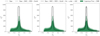Fig. 2. 95% and 99% confidence level constraints on the integrated mass contrast, ΔL, and the comoving size, $r_{\mathrm{L}}^{\mathrm{out}}$, for three different data combinations as compared to the constraints from the Copernican prior convolved with the CMB likelihoods.

The constraining power of future surveys on the radial inhomogeneity can be quantitatively compared to the expectation from the Copernican prior and CMB by comparing the ratio of the 95% confidence regions in the parameter space (see Table 2). Considering all scales, the ratio is always less than one, showing the capability of future surveys to rule out non-Copernican structures. However, at large scales, constraints provided by data still allow for non-Copernican mass density fluctuations since for $r_{\mathrm{L}}^{\mathrm{out}}\ge 190\mathrm{Mpc}$ the ratio is approximately equal to two. We note that, for both cases, the combination Base + DESI + Euclid provides constraints comparable to those obtained from the combination of all data, pointing out the important role that forthcoming LSS surveys will have to test the Copernican principle.

We also consider the case of non-zero background curvature, that is, K_B ≠ 0 in Eq. (10). The result is shown in the last row of Table 2. The inclusion of background curvature degrades the constraints by approximately 10% compared to the flat case, still providing a competitive constraint on the non-Copernican parameters.

5.1.2. Comparison with present-day constraints

In order to quantify the role of future surveys in constraining inhomogeneity around us, we compare our constraints with the ones from current data only, as obtained in Camarena et al. (2021). Specifically, we compute the improvement on the observed area A_obs considering the data combinations presented in Table 3. Our present analyses do not include a cosmic chronometer dataset as contributions of this kind of data are expected to be secondary as compared with SNe and BAOs (Camarena et al. 2021). We note that our previous implementation of such data did not include the full covariance matrix presented in Moresco et al. (2020), revised and discussed in Moresco et al. (2022).

Our Base analysis shows an improvement upon the current constraints by more than 20%, when all scales are considered, and provides an improvement of 28% when compared to the constraints from Base C and Base C + BAO + HZ at scales $r_{\mathrm{L}}^{\mathrm{out}}\ge 190\mathrm{Mpc}$, where HZ denotes the cosmic chronometers dataset used in Camarena et al. (2021). It is interesting to note that our forecast Base analysis provides constraints comparable to those obtained with all the latest cosmological data available, Base C + BAO + HZ + y-dist + kSZ case, showing the importance of forthcoming SN surveys and 1% prior on the Hubble constant.

On the other hand, LSS surveys will play an important role in testing the Copernican principle. As shown in Table 3, future measurements from Euclid and DESI will sharpen the current constraints of Base C by approximately 35%, both at $0\le r_{\mathrm{L}}^{\mathrm{out}}$ and $190\mathrm{Mpc}\le r_{\mathrm{L}}^{\mathrm{out}}$. The inclusion of Euclid and DESI will also tighten the parameter space by more than 30% compared to the combination Base C + BAO + HZ. When compared to the combination Base C + BAO + HZ + y-dist. + kSZ, our analysis with the forthcoming Euclid and DESI data shows an improvement of 26% for $0\le r_{\mathrm{L}}^{\mathrm{out}}$ and 10% for $190\mathrm{Mpc}\le r_{\mathrm{L}}^{\mathrm{out}}$.

Finally, the combination of all data considered here will tighten our current constraints, leading to improvements up to 41% for scales at $190\mathrm{Mpc}\le r_{\mathrm{L}}^{\mathrm{out}}$ and 35% for $0\le r_{\mathrm{L}}^{\mathrm{out}}$ (see Table 3).

5.2. ΛLTB mocks

In Fig. 3 we show the marginalised constraints at the 95% and 99% confidence levels on Δ_C and z_B, for the three ΛLTB fiducial cosmologies, as compared to the constraints coming from the Copernican prior and CMB observations.

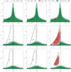Fig. 3. 95% and 99% confidence level constraints on the contrast at the centre, ΔC, and the redshift of the boundary, zB, for the ΛLTB mock catalogues of Table 1 as compared to the constraints from the Copernican prior convolved with the CMB likelihood. The black star is placed at the fiducial values for the LTB parameters, i.e. ΔC = −0.5 and zB = 0.05 (top row, ΛLTB 1), ΔC = −0.1 and zB = 0.4 (middle row, ΛLTB 2), and ΔC = −0.1 and zB = 0.8 (bottom row, ΛLTB 3). We note that the zB axis is not same for all figures.

From the analysis relative to ΛLTB 1 (top row), we can see that future data will be able to probe the local structure. This means that the effect of the cosmic variance on the position of the observer will be reduced thanks to the forthcoming surveys.

On the other hand, from the analysis relative to ΛLTB 2 (middle row) and 3 (bottom row), we see that inhomogeneities that are large, but relatively shallow, can be detected with high significance thanks to future data. More precisely, one can note that our analyses exclude the FLRW case (Δ_C = 0 and z_B = 0) by ≳3σ (pink contours). This stresses the important roles of the next-generation surveys in testing the Copernican principle.

6. Discussion

6.1. The role of large-scale structure data

We have seen from the results of Sect. 5.1 on the ΛCDM mocks that future surveys, such as Euclid, will grant a ≈30% improvement on inhomogeneity around the observer. In particular, for scales greater than 190 Mpc, the combination of all data will constrain inhomogeneity to only 1.7 times the area of the region allowed by standard cosmology. Given the fact that Euclid probes the redshift range 0.9 < z < 1.8, one may wonder if the improvement due to Euclid comes directly from better constraints on the shape of the angular diameter distance and Hubble rate or indirectly from better constraints on the cosmological parameters.

In order to answer the previous question we show in Fig. 4 the fluctuations in the apparent magnitude, Hubble rate and angular diameter distance for the ΛLTB model as compared to the fiducial ΛCDM one. The 68% and 95% bands are obtained by evaluating the relevant functions at every point of the chains. We compare three analyses: the Base one, Base with present BAO and Euclid, and Base with present BAOs and DESI. From this plot, it appears that the shape of the various functions does not change when adding Euclid or DESI. In other words, these two surveys do not improve the constraints in specific redshift ranges but rather they help at tightening the overall uncertainties. From this we conclude that the improvement due to Euclid comes mostly from better constraints on the cosmological parameters, although this works in synergy with DESI and the other observables.

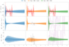Fig. 4. Fluctuations in the apparent magnitude (top row), Hubble rate (middle row), and angular diameter distance (bottom row) for the ΛLTB model as compared to the fiducial ΛCDM one. The 68% and 95% bands are obtained by evaluating the relevant functions at every point of the chains. The red points show LSST and Euclid DESIRE SN data, the black ones Euclid data, and the purple ones DESI data. See Sect. 6.1.

6.2. Beyond the central observer

As mentioned earlier, our aim is to test radial homogeneity around us, neglecting anisotropies. We then placed the observer at the centre of the spherical over/underdensity. However, in an inhomogeneous universe beyond FLRW, neglecting anisotropies could not be justified because anisotropies may affect observables as much as radial inhomogeneities. In other words, the modelling adopted in this work implies a spherically symmetric inhomogeneity and a fine-tuning of the observer’s position.

From the results of Sect. 5.1 on the ΛCDM mocks we see, a posteriori, that large structures with shallow contrasts are allowed by future data. If, for example, we consider a contrast of δ = −0.1, the corresponding change in the Hubble rate is approximately δH₀/H₀ = −f(Ω_m)δ/3 ≃ 0.017, where f ≃ 0.5 is the present-day growth rate for the concordance ΛCDM model. The CMB dipole, if the observer were at, for example, a distance d_obs = 300 Mpc from the centre, using v = ΔH d_obs, is then

$$\begin{array}{c}\hfill \beta =\frac{v}{c}\simeq 1.2\times {10}^{-3},\end{array}$$(21)

which is basically the observed CMB dipole (Planck Collaboration I 2020). As the structures that we consider in this work extend to, at most, 1000 Mpc (see Fig. 2), the required fine-tuning has a chance of less than 1 in 40. In other words, the fine-tuning required to satisfy the CMB dipole is rather mild and therefore the motivation for considering an off-centre observer is to provide a better description of possibly anisotropic data, rather than to relieve the fine-tuning of the observer’s position.

It is worth mentioning that the fine-tuning is instead very severe when considering void models as alternatives to dark energy, a possibility that was not explored here and not favoured by data (see Marra et al. 2022). Indeed, in this case the underdensity has a radius of ≈3 Gpc and δH₀/H₀ ≈ 0.2 so that the observer has to be within ≈30 Mpc from the centre, giving rise to a fine-tuning of one in a million (Marra & Notari 2011). We note, however, as pointed out in Garcia-Bellido & Haugboelle (2008b), that it is possible to alleviate this improbability by displacing the observer and then making them move towards the centre. For distances of a few hundred Mpc and velocities of a few thousand km s⁻¹, the effect is indistinguishable from the observed CMB dipole. In a way, one exchanges an improbability in location for an improbability in the direction of motion. The overall effect is to reduce the coincidence to a few parts in a thousand.

7. Conclusions

Testing fundamental assumptions of cosmology is a crucial step towards improving our understanding of the Universe and firmly establishing the foundations of the standard cosmological paradigm. In this work we have tested the Copernican principle by placing constraints on the ΛLTB model using current and forecast data products. Specifically, we focused on the capability of Euclid to test the Copernican principle in conjunction with data from current and forthcoming surveys, such as SH0ES, DESI, and LSST.

In particular, we compared constraints on the ΛLTB model coming from the forecast and current data against constraints drawn from the Copernican prior–the statistical counterpart of the Copernican principle. This comparison allowed us to quantify how well we can constrain deviations from the Copernican principle.

We have considered two types of fiducial models: the standard ΛCDM model and the inhomogeneous ΛLTB model. By analysing the latter we aimed to determine if next-generation surveys will be able to detect deviations from the Copernican principle, while our analysis of ΛCDM data aimed to investigate if forthcoming data can successfully test the Copernican principle.

We have found that the inclusion of data from Euclid, and other future surveys, will improve the current constraints on the Copernican principle by up to 40%. This improvement will be especially important at scales r_B ≥ 190 Mpc, where the inclusion of Euclid, and other forthcoming surveys, will reduce the constrained area of the space parameters by a factor of < 2 as compared with the area allowed by the Copernican prior. Furthermore, we find that using the forthcoming Euclid data, and data from other future surveys, we will be able to detect inhomogeneous deviations of the FLRW metric, including gigaparsec-scale inhomogeneities of contrast −0.1. Our analyses show that, given the precision of Euclid and other forthcoming surveys, a detection of this kind would allow us to rule out the FLRW space-time (Δ_C = 0 and z_B = 0) by ≳3σ.

Our results rely on the assumption of a particular curvature profile, and, as shown in Appendix A, constraints could be weakened by up to a factor of ∼2 under the assumption of a more general profile. This drawback in our analysis, produced by the choice of a particular curvature profile, could be overcome by introducing data-driven methods that allow us to reconstruct the local distribution of matter in a more robust way. We will implement approaches of this sort in future research.

In summary, this work highlights the importance of synergies between Euclid and external probes in testing the Copernican principle, which is one of the fundamental assumptions of the standard cosmological paradigm.

Acknowledgments

D.C. thanks CAPES for financial support. V.M. thanks C.N.Pq. and FAPES for partial financial support. This project has received funding from the European Union’s Horizon 2020 research and innovation programme under the Marie Skłodowska-Curie grant agreement No. 888258. J.G.B., M.M. and S.N. acknowledge support from the research project PGC2018-094773-B-C32, and the Spanish Research Agency (Agencia Estatal de Investigación) through the Grant IFT Centro de Excelencia Severo Ochoa No. CEX2020-001007-S, funded by MCIN/AEI/10.13039/501100011033. L.L. was supported by a Swiss National Science Foundation Professorship grant (Nos. 170547 and 202671). The work of CJAPM work was financed by FEDER–Fundo Europeu de Desenvolvimento Regional funds through the COMPETE 2020–Operational Programme for Competitiveness and Internationalisation (POCI), and by Portuguese funds through FCT – Fundação para a Ciência e a Tecnologia in the framework of the project POCI-01-0145-FEDER-028987 and PTDC/FIS-AST/28987/2017. M.M. also received support from “la Caixa” Foundation (ID 100010434), with fellowship code LCF/BQ/PI19/11690015. D.S. acknowledges financial support from the Fondecyt Regular project number 1200171. Ad.S. acknowledges the support from the Fundação para a Ciência e a Tecnologia (FCT) through the Investigador FCT Contract No. IF/01135/2015 and POCH/FSE (EC) and in the form of an exploratory project with the same reference. J.P.M. and Ad.S. acknowledge the support from FCT Projects with references EXPL/FIS-AST/1368/2021, PTDC/FIS-AST/0054/2021, UIDB/04434/2020, UIDP/04434/2020, CERN/FIS-PAR/0037/2019, PTDC/FIS-OUT/29048/2017. This work made use of the CHE cluster, managed and funded by COSMO/CBPF/MCTI, with financial support from FINEP and FAPERJ, and operating at the Javier Magnin Computing Center/CBPF. This work also made use of the Virgo Cluster at Cosmo-ufes/UFES, which is funded by FAPES and administrated by Renan Alves de Oliveira. The Euclid Consortium acknowledges the European Space Agency and a number of agencies and institutes that have supported the development of Euclid, in particular the Academy of Finland, the Agenzia Spaziale Italiana, the Belgian Science Policy, the Canadian Euclid Consortium, the French Centre National d’Etudes Spatiales, the Deutsches Zentrum für Luft- und Raumfahrt, the Danish Space Research Institute, the Fundação para a Ciência e a Tecnologia, the Ministerio de Ciencia e Innovación, the National Aeronautics and Space Administration, the National Astronomical Observatory of Japan, the Netherlandse Onderzoekschool Voor Astronomie, the Norwegian Space Agency, the Romanian Space Agency, the State Secretariat for Education, Research and Innovation (SERI) at the Swiss Space Office (SSO), and the United Kingdom Space Agency. A complete and detailed list is available on the Euclid website (http://www.euclid-ec.org).

References

Appendix A: The curvature profile

The analyses presented in this paper rely on the assumption of the compensated profile introduced in Sect. 2.2, which was chosen in order to ensure that the ΛCDM background is recovered at r ≥ r_B, a crucial feature in order to confront CMB data consistently using an effective FLRW model.

Here, we compare our model to the Garcia-Bellido and Haugboelle (GBH) model (Garcia-Bellido & Haugboelle 2008a), which parametrises the LTB metric by imposing

$$\begin{array}{cc}\hfill {\mathrm{\Omega }}_{\mathrm{m},0}(r)& ={\mathrm{\Omega }}_{\mathrm{m},0}^{\mathrm{out}}+({\mathrm{\Omega }}_{\mathrm{m},0}^{\mathrm{in}}-{\mathrm{\Omega }}_{\mathrm{m},0}^{\mathrm{out}})\left\{\frac{1-tanh[(r-r_0)/2\mathrm{\Delta }r]}{1+tanh[r_0/2\mathrm{\Delta }r]}\right\},\hfill \\ \hfill H_0(r)& =H_{\perp 0}^{\mathrm{out}}+(H_{\perp 0}^{\mathrm{in}}-H_{\perp 0}^{\mathrm{out}})\left\{\frac{1-tanh[(r-r_0)/2\mathrm{\Delta }r]}{1+tanh[r_0/2\mathrm{\Delta }r]}\right\},\hfill \end{array}$$

where r₀ is the size of the void, Δr the transition scale, ${\mathrm{\Omega }}_{\mathrm{m},0}^{\mathrm{in}}\equiv {\mathrm{\Omega }}_{\mathrm{m},0}(r=0)$, and $H_{\perp 0}^{\mathrm{in}}\equiv H_{\perp 0}(r=0)$. Fig. A.1 shows the differences between our model (solid blue line) and the GBH model, where we have adopted r₀ = r_L (dotted green line) and r₀ = r_B (dashed red line). When the size of the GBH inhomogeneity is fixed to r_B, a scale greater that r_B is needed to recover the ΛCDM background. On the other hand, if one assumes r₀ = r_L, the GBH model tends to the ΛCDM background at r = r_B. In contrast, our model perfectly matches the ΛCDM background at any scale r ≥ r_B. The compensating behaviour of our model is particularly notable in the top panel of the Fig. A.1, where we note that $\delta (r_{\mathrm{L}}^{\mathrm{out}},t_0)=\delta (r_{\mathrm{B}}^{\mathrm{out}},t_0)=0$ for our model while the GBH models does not satisfy δ(r^out, t₀) = 0 for all $r^{\mathrm{out}}\ge r_{\mathrm{B}}^{\mathrm{out}}$.

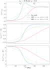Fig. A.1. Comparison between our model and the GBH parametrization. Top: Density contrast of matter today, δ(r, t0), as a function of the FLRW comoving coordinate. Our compensated model (solid blue line) satisfies $\delta (r_{\mathrm{L}}^{\mathrm{out}},t_0)=\delta (r_{\mathrm{B}}^{\mathrm{out}},t_0)=0$, while the ΛCDM background is not exactly recovered for the GBH models (dashed red and dotted green lines). Middle: Deviations from the background density of matter, ${\mathrm{\Omega }}_{\mathrm{m},0}^{\mathrm{out}}$, as a function of the FLRW comoving coordinate. The GBH model with r0 = rB (red dashed line) largely deviates from ${\mathrm{\Omega }}_{\mathrm{m},0}^{\mathrm{out}}$ at $r^{\mathrm{out}}=r_{\mathrm{B}}^{\mathrm{out}}$. On the other hand, the choice of r0 = rL for the GBH leads to deviations of approximately −0.01 from the background at $r^{\mathrm{out}}=r_{\mathrm{B}}^{\mathrm{out}}$. The model assumed in this work fully recovers ${\mathrm{\Omega }}_{\mathrm{m},0}^{\mathrm{out}}$ at any $r^{\mathrm{out}}\ge r_{\mathrm{B}}^{\mathrm{out}}$. Bottom: Deviations from the background Hubble expansion as a function of the FLRW comoving coordinate. GBH models (dashed red and dotted green lines) do not perfectly match the ΛCDM background expansion history at $r^{\mathrm{out}}=r_{\mathrm{B}}^{\mathrm{out}}$.

Furthermore, to investigate the dependence of our results on the chosen profile, we performed an additional analysis using the following generalisation of Eq. (10):

$$\begin{array}{c}\hfill P_3(x,\alpha )=\{\begin{array}{cc}1\hfill & \mathrm{for}0\le x<\alpha \hfill \\ 1-exp[-\frac{1-\alpha }{x-\alpha }{(1-\frac{x-\alpha }{1-\alpha })}^3]\hfill & \mathrm{for}\alpha \le x<1\hfill \\ 0\hfill & \mathrm{for}1\le x\hfill \end{array},\end{array}$$(A.1)

with 0 < α < 1. This new parameter will modify the smoothness of the transition between the inner and compensating region, leading to sharpened profiles when α approximates to 1. Results from this extra analysis, which is performed using the combination Base + BAO + Euclid + DESI + y-dist. + kSZ from the ΛCDM fiducial, shows that the inclusion of the α parameter weakens the constraints on Δ_C and $r_{\mathrm{L}}^{\mathrm{out}}$ by a factor of two, compared to the results from Eq. (10).

Appendix B: Re-scaling datasets

Covariance matrices are fundamental pieces of forecast analyses. However, their production for forthcoming surveys is an open issue when non-standard cosmologies are considered (Harnois-Deraps et al. 2019; Friedrich et al. 2021; Ferreira & Marra 2022). This complicates the construction of forecast data for ΛLTB cosmologies. Nesseris et al. (2022) has overcome this issue by neglecting the error due to the non-standard cosmology. Here, we apply a re-scaling method to convert the ΛCDM forecast data and its covariance matrices into ΛLTB catalogues.

Consider a given dataset, with x_i being the observed quantity, z_i the corresponding redshift, and C_ij the covariance matrix. This dataset can be re-scaled to agree with a particular model via the following steps.

First, we define R_ij = C_ij/x_ix_j, a new matrix that contains the relative uncertainties and correlations from the original covariance matrix. Second, we compute with the theoretical prediction of the new model the fiducial values at the relevant redshifts, such that $x_i^{\text{f}}\equiv x^{\text{fid}}(z_i)$. Third, using the above defined quantities, we compute the new correlation matrix as ${\stackrel{\sim }{C}}_{\mathit{ij}}=x_i^{\mathrm{f}}{x}_j^{\mathrm{f}}{R}_{\mathit{ij}}$. Finally, we then draw a random realisation, ${\stackrel{\sim }{x}}_i$, of the multivariate-normal distribution $\mathcal{N}(x_i^{\mathrm{f}},{\stackrel{\sim }{C}}_{\mathit{ij}})$.

We note that this method assumes that relative error and correlations are not changed by a non-standard model. As discussed through this paper, the procedure above is also applied to re-scale real data according the fiducial models presented on Table 1; this ensures that all data are consistently described by a particular fiducial model.

Appendix C: The inhomogeneous Hubble constant

The ΛLTB model features a profile function H₀(r) that depends on the radial distance from the centre of the void, instead of a constant value like H₀ in the ΛCDM model. Since there is not a preferable scale to set the rate of expansion of the Universe, the definition of H₀ remains arbitrary. To overcome this issue, we extend the FLRW definitions and mimic the observational procedure to locally constrain the Hubble constant. Explicitly, we adopt the definition $H_0^{\text{L}}$ for inhomogeneous cosmological models that was introduced in Camarena et al. (2022). This method, which is applied for every sample point of the parameter space, follows the following steps.

First, we create a mock catalogue using the redshifts of Pantheon SNe at 0.023 < z < 0.15 and the ΛLTB luminosity distances at the corresponding redshifts. Second, the mock data are fitted using an extension of the cosmographic expansion given by

$$\begin{array}{cc}\hfill D_{\mathrm{L}}(z)& =\frac{\mathit{cz}}{H_0^{\mathrm{L}}}[1+\frac{(1-q_0^r)z}{2}],\hfill \end{array}$$(C.1)

$$\begin{array}{cc}\hfill q_0^r(r)& =[\frac{{\mathrm{\Omega }}_{\mathrm{m}}(r)}{2}-{\mathrm{\Omega }}_{\mathrm{\Lambda }}(r)]{\left[\frac{H_0(r)}{H_0^{\mathrm{L}}}\right]}^2,\hfill \end{array}$$(C.2)

where $q_0^r$ is the radial-dependent deceleration parameter. Finally, the best-fit value of $H_0^{\text{L}}$ is adopted as the measured Hubble constant.

It is interesting to point out that this procedure mimics the standard cosmic distance ladder analysis of SNe that follow the Hubble flow, while taking into account the effect of the inhomogeneity on the measurement of the Hubble constant. We note that other authors have previously proposed similar approximations (Redlich et al. 2014; Efstathiou 2021).

All Tables

All Figures

Fig. 1. Several ΛLTB quantities as a function of the FLRW comoving coordinate rout. Top: density contrast of matter, δ(r) = ρm(r, t0)/ρm(rB, t0)−1, and integrated mass, Δ(r), as functions of the FLRW comoving coordinate. At radius $r_{\mathrm{L}}^{\mathrm{out}}$ the central structure ends and the compensating shell begins, while $r_{\mathrm{B}}^{\mathrm{out}}$ is the boundary of the spherical inhomogeneity. Middle: deviations from the background density of matter, ${\mathrm{\Omega }}_{\mathrm{m},0}^{\mathrm{out}}$, and curvature, ${\mathrm{\Omega }}_{k,0}^{\mathrm{out}}$, as a function of the FLRW comoving coordinate due to the radial dependence on Ωm, 0(r) and Ωk, 0(r). We note that the FLRW background quantities are recovered for $r\ge r_{\mathrm{B}}^{\mathrm{out}}$. Bottom: transverse and longitudinal fluctuations in the expansion rates as a function of the FLRW comoving coordinate.

In the text

	Fig. 2. 95% and 99% confidence level constraints on the integrated mass contrast, ΔL, and the comoving size, $r_{\mathrm{L}}^{\mathrm{out}}$, for three different data combinations as compared to the constraints from the Copernican prior convolved with the CMB likelihoods.
In the text

Fig. 3. 95% and 99% confidence level constraints on the contrast at the centre, ΔC, and the redshift of the boundary, zB, for the ΛLTB mock catalogues of Table 1 as compared to the constraints from the Copernican prior convolved with the CMB likelihood. The black star is placed at the fiducial values for the LTB parameters, i.e. ΔC = −0.5 and zB = 0.05 (top row, ΛLTB 1), ΔC = −0.1 and zB = 0.4 (middle row, ΛLTB 2), and ΔC = −0.1 and zB = 0.8 (bottom row, ΛLTB 3). We note that the zB axis is not same for all figures.

In the text

Fig. 4. Fluctuations in the apparent magnitude (top row), Hubble rate (middle row), and angular diameter distance (bottom row) for the ΛLTB model as compared to the fiducial ΛCDM one. The 68% and 95% bands are obtained by evaluating the relevant functions at every point of the chains. The red points show LSST and Euclid DESIRE SN data, the black ones Euclid data, and the purple ones DESI data. See Sect. 6.1.

In the text

Fig. A.1. Comparison between our model and the GBH parametrization. Top: Density contrast of matter today, δ(r, t0), as a function of the FLRW comoving coordinate. Our compensated model (solid blue line) satisfies $\delta (r_{\mathrm{L}}^{\mathrm{out}},t_0)=\delta (r_{\mathrm{B}}^{\mathrm{out}},t_0)=0$, while the ΛCDM background is not exactly recovered for the GBH models (dashed red and dotted green lines). Middle: Deviations from the background density of matter, ${\mathrm{\Omega }}_{\mathrm{m},0}^{\mathrm{out}}$, as a function of the FLRW comoving coordinate. The GBH model with r0 = rB (red dashed line) largely deviates from ${\mathrm{\Omega }}_{\mathrm{m},0}^{\mathrm{out}}$ at $r^{\mathrm{out}}=r_{\mathrm{B}}^{\mathrm{out}}$. On the other hand, the choice of r0 = rL for the GBH leads to deviations of approximately −0.01 from the background at $r^{\mathrm{out}}=r_{\mathrm{B}}^{\mathrm{out}}$. The model assumed in this work fully recovers ${\mathrm{\Omega }}_{\mathrm{m},0}^{\mathrm{out}}$ at any $r^{\mathrm{out}}\ge r_{\mathrm{B}}^{\mathrm{out}}$. Bottom: Deviations from the background Hubble expansion as a function of the FLRW comoving coordinate. GBH models (dashed red and dotted green lines) do not perfectly match the ΛCDM background expansion history at $r^{\mathrm{out}}=r_{\mathrm{B}}^{\mathrm{out}}$.

In the text

References

- Alam, S., Ata, M., Bailey, S., et al. 2017, MNRAS, 470, 2617 [Google Scholar]
- Albrecht, A., Bernstein, G., Cahn, R., et al. 2006, arXiv e-prints [arXiv:astro-ph/0609591] [Google Scholar]
- Aluri, P. K., Cea, P., Chingangbam, P., et al. 2022, arXiv e-prints [arXiv:2207.05765] [Google Scholar]
- Amendola, L., Appleby, S., Avgoustidis, A., et al. 2018, Liv. Rev. Relat., 21, A2 [NASA ADS] [Google Scholar]
- Astier, P., Balland, C., Brescia, M., et al. 2014, A&A, 572, A80 [NASA ADS] [CrossRef] [EDP Sciences] [Google Scholar]
- Audren, B., Lesgourgues, J., Benabed, K., & Prunet, S. 2013, JCAP, 1302, 001 [Google Scholar]
- Ben-Dayan, I., Gasperini, M., Marozzi, G., Nugier, F., & Veneziano, G. 2013, JCAP, 06, 002 [CrossRef] [Google Scholar]
- Bengaly, C. A. P., Maartens, R., & Santos, M. G. 2018, JCAP, 04, 031 [CrossRef] [Google Scholar]
- Beutler, F., Blake, C., Colless, M., et al. 2011, MNRAS, 416, 3017 [NASA ADS] [CrossRef] [Google Scholar]
- Blas, D., Lesgourgues, J., & Tram, T. 2011, JCAP, 07, 034 [CrossRef] [Google Scholar]
- Brinckmann, T., & Lesgourgues, J. 2019, Phys. Dark Univ., 24, 100260 [Google Scholar]
- Camarena, D., Marra, V., Sakr, Z., & Clarkson, C. 2021, MNRAS, 509, 1291 [NASA ADS] [CrossRef] [Google Scholar]
- Camarena, D., Marra, V., Sakr, Z., & Clarkson, C. 2022, Class. Quant. Grav., 39, 184001 [NASA ADS] [CrossRef] [Google Scholar]
- Carrick, J., Turnbull, S. J., Lavaux, G., & Hudson, M. J. 2015, MNRAS, 450, 317 [Google Scholar]
- Chen, L., Huang, Q.-G., & Wang, K. 2019, JCAP, 02, 028 [CrossRef] [Google Scholar]
- Colin, J., Mohayaee, R., Sarkar, S., & Shafieloo, A. 2011, MNRAS, 414, 264 [Google Scholar]
- Colin, J., Mohayaee, R., Rameez, M., & Sarkar, S. 2017, MNRAS, 471, 1045 [Google Scholar]
- Cropper, M., Pottinger, S., Azzollini, R., et al. 2018, Proc. SPIE Int. Soc. Opt. Eng., 10698, 1069828 [NASA ADS] [Google Scholar]
- Dalang, C., & Bonvin, C. 2022, MNRAS, 512, 3895 [NASA ADS] [CrossRef] [Google Scholar]
- de la Torre, S., & Guzzo, L. 2012, MNRAS, 427, 327 [NASA ADS] [CrossRef] [Google Scholar]
- DESI Collaboration (Aghamousa, A., et al.) 2016, arXiv e-prints [arXiv:1611.00036] [Google Scholar]
- du Mas des Bourboux, H., Rich, J., Font-Ribera, A., et al. 2020, ApJ, 901, 153 [CrossRef] [Google Scholar]
- Efstathiou, G. 2021, MNRAS, 505, 3866 [NASA ADS] [CrossRef] [Google Scholar]
- Euclid Collaboration (Blanchard, A., et al.) 2020a, A&A, 642, A191 [NASA ADS] [CrossRef] [EDP Sciences] [Google Scholar]
- Euclid Collaboration (Paykari, P., et al.) 2020b, A&A, 635, A139 [NASA ADS] [CrossRef] [EDP Sciences] [Google Scholar]
- Euclid Collaboration (Scaramella, R., et al.) 2022, A&A, 662, A112 [NASA ADS] [CrossRef] [EDP Sciences] [Google Scholar]
- February, S., Larena, J., Smith, M., & Clarkson, C. 2010, MNRAS, 405, 2231 [NASA ADS] [Google Scholar]
- Feindt, U., Kerschhaggl, M., Kowalski, M., et al. 2013, A&A, 560, A90 [NASA ADS] [CrossRef] [EDP Sciences] [Google Scholar]
- Ferreira, P. D. S., & Quartin, M. 2021, Phys. Rev. Lett., 127, 101301 [NASA ADS] [CrossRef] [Google Scholar]
- Ferreira, T., & Marra, V. 2022, MNRAS, 513, 5438 [NASA ADS] [Google Scholar]
- Fixsen, D., Cheng, E., Gales, J., et al. 1996, ApJ, 473, 576 [NASA ADS] [CrossRef] [Google Scholar]
- Font-Ribera, A., McDonald, P., Mostek, N., et al. 2014, JCAP, 05, 023 [CrossRef] [Google Scholar]
- Friedrich, O., Andrade-Oliveira, F., Camacho, H., et al. 2021, MNRAS, 508, 3125 [NASA ADS] [CrossRef] [Google Scholar]
- Garcia-Bellido, J., & Haugboelle, T. 2008a, JCAP, 04, 003 [CrossRef] [Google Scholar]
- Garcia-Bellido, J., & Haugboelle, T. 2008b, JCAP, 09, 016 [CrossRef] [Google Scholar]
- Gong, Y., Cooray, A., & Chen, X. 2010, ApJ, 709, 1420 [NASA ADS] [CrossRef] [Google Scholar]
- Harnois-Deraps, J., Giblin, B., & Joachimi, B. 2019, A&A, 631, A160 [NASA ADS] [CrossRef] [EDP Sciences] [Google Scholar]
- Hudson, M. J., Smith, R. J., Lucey, J. R., & Branchini, E. 2004, MNRAS, 352, 61 [Google Scholar]
- Ishak, M., Peel, A., & Troxel, M. A. 2013, Phys. Rev. Lett., 111, 251302 [NASA ADS] [CrossRef] [Google Scholar]
- Jonsson, J., Sullivan, M., Hook, I., et al. 2010, MNRAS, 405, 535 [NASA ADS] [Google Scholar]
- Kim, Y., Park, C.-G., Noh, H., & Hwang, J.-C. 2022, A&A, 660, A139 [NASA ADS] [CrossRef] [EDP Sciences] [Google Scholar]
- Kronborg, T., Hardin, D., Guy, J., et al. 2010, A&A, 514, A44 [NASA ADS] [CrossRef] [EDP Sciences] [Google Scholar]
- Laureijs, R., Amiaux, J., Arduini, S., et al. 2011, arXiv e-prints [arXiv:1110.3193] [Google Scholar]
- Lewis, A. 2019, arXiv e-prints [arXiv:1910.13970] [Google Scholar]
- LSST Science Collaboration (Abell, P. A., et al.) 2009, arXiv e-prints [arXiv:0912.0201] [Google Scholar]
- Lyke, B. W., Higley, A. N., McLane, J. N., et al. 2020, ApJS, 250, 8 [NASA ADS] [CrossRef] [Google Scholar]
- Maciaszek, T., Ealet, A., Jahnke, K., et al. 2016, SPIE Conf. Ser., 9904, 99040T [NASA ADS] [Google Scholar]
- Marra, V., & Notari, A. 2011, Class. Quant. Grav., 28, 164004 [NASA ADS] [CrossRef] [Google Scholar]
- Marra, V., Quartin, M., & Amendola, L. 2013, Phys. Rev. D, 88, 063004 [NASA ADS] [CrossRef] [Google Scholar]
- Marra, V., Castro, T., Camarena, D., Borgani, S., & Ragagnin, A. 2022, A&A, 664, A179 [NASA ADS] [CrossRef] [EDP Sciences] [Google Scholar]
- Martinelli, M., Martins, C. J. A. P., Nesseris, S., et al. 2020, A&A, 644, A80 [NASA ADS] [CrossRef] [EDP Sciences] [Google Scholar]
- Martinelli, M., Martins, C. J. A. P., Nesseris, S., et al. 2021, A&A, 654, A148 [NASA ADS] [CrossRef] [EDP Sciences] [Google Scholar]
- Migkas, K., Schellenberger, G., Reiprich, T. H., et al. 2020, A&A, 636, A15 [NASA ADS] [CrossRef] [EDP Sciences] [Google Scholar]
- Migkas, K., Pacaud, F., Schellenberger, G., et al. 2021, A&A, 649, A151 [NASA ADS] [CrossRef] [EDP Sciences] [Google Scholar]
- Mohayaee, R., Rameez, M., & Sarkar, S. 2021, Eur. Phys. J. Spec. Top., 230, 2067 [NASA ADS] [CrossRef] [Google Scholar]
- Moresco, M., Jimenez, R., Verde, L., Cimatti, A., & Pozzetti, L. 2020, ApJ, 898, 82 [NASA ADS] [CrossRef] [Google Scholar]
- Moresco, M., Amati, L., Amendola, L., et al. 2022, Living Rev. Relativ., 25, 6 [NASA ADS] [CrossRef] [Google Scholar]
- Moss, A., Zibin, J. P., & Scott, D. 2011, Phys. Rev. D, 83, 103515 [NASA ADS] [CrossRef] [Google Scholar]
- Nesseris, S., Sapone, D., Martinelli, M., et al. 2022, A&A, 660, A67 [NASA ADS] [CrossRef] [EDP Sciences] [Google Scholar]
- Planck Collaboration XXVII. 2014, A&A, 571, A27 [NASA ADS] [CrossRef] [EDP Sciences] [Google Scholar]
- Planck Collaboration I. 2020, A&A, 641, A1 [Google Scholar]
- Planck Collaboration VI. 2020, A&A, 641, A6 [Erratum: A&A 652, C4 (2021)] [NASA ADS] [CrossRef] [EDP Sciences] [Google Scholar]
- Planck Collaboration Int. LVI. 2020, A&A, 644, A100 [EDP Sciences] [Google Scholar]
- Pozzetti, L., Hirata, C. M., Geach, J. E., et al. 2016, A&A, 590, A3 [NASA ADS] [CrossRef] [EDP Sciences] [Google Scholar]
- Prieto, E., Amiaux, J., Auguères, J. L., et al. 2012, SPIE Conf. Ser., 8442, 84420W [NASA ADS] [Google Scholar]
- Quartin, M., Marra, V., & Amendola, L. 2014, Phys. Rev. D, 89, 023009 [NASA ADS] [CrossRef] [Google Scholar]
- Rahman, W., Trotta, R., Boruah, S. S., Hudson, M. J., & van Dyk, D. A. 2022, MNRAS, 514, 139 [NASA ADS] [CrossRef] [Google Scholar]
- Raichoor, A., de Mattia, A., Ross, A. J., et al. 2020, MNRAS, 500, 3254 [NASA ADS] [CrossRef] [Google Scholar]
- Redlich, M., Bolejko, K., Meyer, S., Lewis, G. F., & Bartelmann, M. 2014, A&A, 570, A63 [NASA ADS] [CrossRef] [EDP Sciences] [Google Scholar]
- Reichardt, C. L., Patil, S., Ade, P. A. R., et al. 2021, ApJ, 908, 199 [NASA ADS] [CrossRef] [Google Scholar]
- Ross, A. J., Samushia, L., Howlett, C., et al. 2015, MNRAS, 449, 835 [NASA ADS] [CrossRef] [Google Scholar]
- Ross, A. J., Bautista, J., Tojeiro, R., et al. 2020, MNRAS, 498, 2354 [NASA ADS] [CrossRef] [Google Scholar]
- Saha, S., Shaikh, S., Mukherjee, S., Souradeep, T., & Wandelt, B. D. 2021, JCAP, 10, 072 [CrossRef] [Google Scholar]
- Scolnic, D., Jones, D. O., Rest, A., et al. 2018, ApJ, 859, 101 [NASA ADS] [CrossRef] [Google Scholar]
- Secrest, N. J., von Hausegger, S., Rameez, M., et al. 2021, ApJ, 908, L51 [Google Scholar]
- Siewert, T. M., Schmidt-Rubart, M., & Schwarz, D. J. 2021, A&A, 653, A9 [NASA ADS] [CrossRef] [EDP Sciences] [Google Scholar]
- Silk, J. 1977, A&A, 59, 53 [NASA ADS] [Google Scholar]
- Valkenburg, W. 2012, Gen. Relat. Gravit., 44, 2449 [CrossRef] [Google Scholar]
- Valkenburg, W., Marra, V., & Clarkson, C. 2014, MNRAS, 438, L6 [CrossRef] [Google Scholar]
- Wang, Y., Chuang, C.-H., & Hirata, C. M. 2013, MNRAS, 430, 2446 [NASA ADS] [CrossRef] [Google Scholar]
- Yadav, J. K., Bagla, J. S., & Khandai, N. 2010, MNRAS, 405, 2009 [NASA ADS] [Google Scholar]
- Zibin, J. P. 2008, Phys. Rev. D, 78, 043504 [NASA ADS] [CrossRef] [Google Scholar]