| Issue |
A&A
Volume 699, July 2025
|
|
|---|---|---|
| Article Number | A131 | |
| Number of page(s) | 20 | |
| Section | Cosmology (including clusters of galaxies) | |
| DOI | https://doi.org/10.1051/0004-6361/202554456 | |
| Published online | 04 July 2025 | |
Detecting galaxy – 21-cm cross-correlation during reionization
1
Scuola Normale Superiore di Pisa, Piazza dei Cavallieri 7, 56126 Pisa, Italy
2
Centro Nazionale “High Performance Computing, Big Data and Quantum Computing”, Via Magnanelli 40033 Casalecchio di Reno, Italy
⋆ Corresponding author: samuel.gagnonhartman@sns.it
Received:
10
March
2025
Accepted:
13
May
2025
The cosmic 21-cm signal promises to revolutionize studies of the Epoch of Reionization (EoR). Radio interferometers are aiming for a preliminary, low signal-to-noise (S/N) detection of the 21-cm power spectrum. Cross-correlating 21-cm with galaxies will be especially useful in these efforts, providing both a sanity check for initial 21-cm detection claims and potentially increasing the S/N due to uncorrelated residual systematics. Here we self-consistently simulate large-scale (1 Gpc3) galaxy and 21-cm fields, computing their cross-power spectra for various choices of instruments and survey properties. We use 1080 h observations with SKA-low AA* and HERA-350 as our benchmark 21-cm observations. We create mock Lyman-α narrow-band, slitless and slit spectroscopic surveys, using benchmarks from instruments such as Subaru HyperSupremeCam, Roman grism, VLT MOONS, ELT MOSAIC, and JWST NIRCam. We forecast the resulting S/N of the galaxy–21-cm cross-power spectrum, varying for each pair of instruments the galaxy survey area, depth, and the 21-cm foreground contaminated region of Fourier space. We find that the highest S/N is achievable through slitless, wide-area spectroscopic surveys, with the proposed Roman HLS survey resulting in a ∼55σ (∼13σ) detection of the cross-power with 21-cm as observed with SKA-low AA* (HERA-350), for our fiducial model and assuming ∼500 sq. deg. of overlap. Narrow-band dropout surveys are unlikely to result in a detectable cross-power, due to their poor redshift localization. Slit spectroscopy can provide a high S/N detection of the cross-power for SKA-low AA* observations. Specifically, the planned MOONRISE survey with MOONS on the VLT can result in a ∼3σ detection, while a survey of comparable observing time using MOSAIC on the ELT can result in a ∼4σ detection. Our results can be used to guide survey strategies, facilitating the detection of the galaxy–21-cm cross-power spectrum.
Key words: galaxies: high-redshift / dark ages, reionization, first stars
© The Authors 2025
 Open Access article, published by EDP Sciences, under the terms of the Creative Commons Attribution License (https://creativecommons.org/licenses/by/4.0), which permits unrestricted use, distribution, and reproduction in any medium, provided the original work is properly cited.
This article is published in open access under the Subscribe to Open model. Subscribe to A&A to support open access publication.
1. Introduction
The 21-cm signal from neutral hydrogen is arguably the most promising probe of the Cosmic Dawn (CD) and the Epoch of Reionization (EoR): two of the last remaining frontiers in modern cosmology. The signal holds imprints of the physics of the first galaxies (e.g., Mirocha & Furlanetto 2019; Park et al. 2019), the nature of dark matter (e.g., Clark et al. 2018; Villanueva-Domingo 2021; Facchinetti et al. 2024), and perhaps even the role of dark energy (e.g., Adi et al. 2025) during this crucial period in the development of the Universe.
A number of challenges riddle the path toward a measurement of the 21-cm power spectrum. The interferometer arrays used in tomographic experiments introduce numerous systematic effects into their measurements, all of which must be carefully characterized and accounted for (e.g., Kern et al. 2020; Rath et al. 2024). Furthermore, the highly redshifted 21-cm signal occupies the same radio band as Galactic synchrotron radiation, which overwhelms the cosmic signal by several orders of magnitude. There is also terrestrial contamination to contend with, including radio-frequency interference and the Earth's ionosphere (e.g., Liu & Shaw 2020).
Owing to these challenges, any claim of a detection of the 21-cm power spectrum will require some form of confirmation in order to gain the trust of the scientific community. The most effective method to bolster confidence in a cosmic 21-cm detection is to correlate it with a signal of known cosmic origin.
In addition to building confidence, a cross-correlation signal could even increase the signal-to-noise (S/N) of a detection, because the foregrounds of the two signals are probably not correlated. Several low-redshift studies have indeed confirmed measurements of the 21-cm signal through cross-correlation with galaxy/quasi-stellar object surveys spanning the same volume (e.g., the Green Bank Telescope; Masui et al. 2013, Parkes Radio Telescope; Anderson et al. 2018, MeerKAT; Cunnington et al. 2023, CHIME; Amiri et al. 2024; CHIME Collaboration 2023). Depending on its nature, the cross-power spectrum could also probe the interaction between galaxies and the intergalactic medium (IGM), yielding complementary information to the auto-power spectra (e.g., Hutter et al. 2023; Moriwaki et al. 2024).
For the EoR / CD 21-cm signal at z≳5, there are three main candidates for cross-correlation: cosmic backgrounds, intensity maps, and galaxy surveys, each with its own benefits and challenges. The cosmic microwave background (CMB) is a very well established signal and can cross correlate with the 21-cm signal through secondary anisotropies such as the kinetic Sunyaev-Zel’dovich effect (e.g., Reichardt et al. 2021; Adachi et al. 2022). It is an integral (2D) signal, however, and the lack of line-of-sight modes causes them to correlate only weakly with the cosmic 21-cm signal (e.g., Lidz et al. 2009; Mao 2014; Ma et al. 2018; Vrbanec et al. 2020; La Plante et al. 2022; Sun et al. 2025). On the other hand, line-intensity maps (LIMs) of other emission lines are expected to correlate very strongly with the cosmic 21-cm signal. Most LIMs target metals in the interstellar medium, however, such as CO and CII, whose corresponding luminosities and achievable S/N of the cross-correlation with 21-cm are very uncertain at z≳5 (e.g., Crites et al. 2014; Cooray et al. 2016; Kovetz et al. 2017; Parshley et al. 2018; Heneka & Cooray 2021; Moriwaki & Yoshida 2021; Yang et al. 2022; Pallottini & Ferrara 2023; Fronenberg & Liu 2024).
While LIM experiments will take time to mature, the galaxy mapping toolkit is not only well established but booming at the time of writing. A plethora of ground and space instruments (e.g., the James Webb Space Telescope, the Subaru Telescope, the Atacama Large Millimeter Array) are currently detecting galaxies deep in the EoR. While time-consuming to produce, spectroscopic maps probe the line-of-sight modes crucial for cross-correlation with the cosmic 21-cm signal while avoiding the challenges associated with LIM (Sobacchi et al. 2016; Hutter et al. 2017; Kubota et al. 2020; Vrbanec et al. 2020; La Plante et al. 2023). As the drivers of reionization, galaxies are tightly correlated with ionized bubbles (see Figure 1). Given a sufficient number of galaxies, we should thus detect a strong (anti-) correlation with the 21-cm emitting neutral IGM during the EoR.
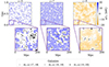 |
Fig. 1. An example 21-cm brightness temperature field at shown at redshifts 6, 7, and 8 (left to right) with galaxies overlaid on zoomed insets (black). Detectable galaxies at these redshifts preferentially reside in ionized regions, with the brightest, most biased galaxies residing in the largest ionized bubbles. The top row shows slices of the full gigaparsec volume used in this study, while the bottom row zooms into a 200 Mpc corner for clarity. Both the brightness temperature and galaxy fields were generated simultaneously using 21cmFASTv4. |
We quantify the detectability of the cross-power spectrum between the 21-cm signal and a galaxy survey spanning the same volume. To do this, we self-consistently simulate large-scale (1 Gpc) maps of the 21-cm brightness temperature and the underlying galaxy field. Using empirical relations that include scatter, we made mock observations of galaxy maps with selection based on Lyman-α and other nebular lines. We quantified the S/N of the galaxy–21-cm cross-power as a function of galaxy survey depth, angular extent, and spectral resolution, as well as the level of foreground contamination of the cosmic 21-cm signal. Based on these estimates, we forecast the S/N for current and upcoming telescopes, including HERA and SKA for 21-cm, and Subaru, Roman, MOONS and MOSAIC for galaxy maps. We conclude with specific recommendations for surveys seeking to maximize the probability of detecting the galaxy–21-cm cross-power spectrum.
The paper is organized as follows. In Section 2 we present our cosmological simulations. In Section 3 we convert our simulation outputs into a mock signal. This involves various assumptions about instrumental effects and sources of systematic uncertainty. In Section 4 we discuss fiducial instruments and the survey choices we varied to quantify the detectability of the cross-power spectrum. We present our results in Section 5. We conclude in Section 6 with specific recommendations for surveys seeking to detect the cross-power. We assume a standard ΛCDM cosmology with parameters consistent with the latest Planck estimates throughout, wherein H0 = 67.66 km s−1 Mpc−1, Ωm = 0.30966, Ωb = 0.04897, Ωk = 0.0, ΩΛ = 0.68846, and σ8 = 0.8102. Unless stated otherwise, all lengths are quoted in comoving units.
2. Simulating the cosmic signal
The cosmic signal in this study refers to two fields: the 21-cm brightness temperature and an overlapping galaxy map. To simulate the two fields, we used the latest version of the public code 21cmFAST (Mesinger & Furlanetto 2007; Mesinger et al. 2011). We then postprocessed the cosmic signals, added telescope noise, removed foreground-contaminated regions, and implemented selection criteria for galaxy surveys. This section is split into two subsections; the first subsection summarizes how the latest version of 21cmFAST computes cosmological fields and the second subsection discusses our procedure for applying the appropriate observational selection criterion to our simulated galaxy maps.
2.1. Cosmological simulations
We used the latest public release, 21cmFASTv41 (Davies et al. 2025), which allows for greater flexibility in characterizing high-redshift galaxies. We describe the simulation below with a focus on the new galaxy source model. For further information, we refer to Davies et al. (2025).
21cmFAST creates a 3D realization of the matter field at z = 30, evolving it to lower redshifts through second-order Lagrangian perturbation theory (2LPT). We used simulation boxes that are 1 Gpc on a side, with initial conditions sampled on a 11003 grid. This was subsequently down-sampled to a cell size of 2 Mpc. In the previous default version of 21cmFAST, the source fields driving heating and ionization were calculated on filtered versions of the evolved density grid according to the excursion set algorithm (Mesinger et al. 2011). In the default settings, galaxies were not localized on the Eulerian grid. While 21cmFAST has the option to use a discrete halo field via a Lagrangian halo finder named DexM, this algorithm samples over scales with a minimum mass that is set using the size of the grid cell. This renders it prohibitively slow for halos with a mass of Mh≤1010 M⊙ (Mesinger & Furlanetto 2007).
The new model of Davies et al. (2025) uses a combination of Lagrangian halo-finding and coarse time-step merger trees to rapidly build 3D realizations of dark matter halos throughout the EoR/CD. These halos are then populated by galaxies whose properties are sampled from empirical relations conditional on their halo mass and other properties. 21cmFASTv4 therefore explicitly accounts for stochastic galaxy formation and generates 3D lightcones of galaxy properties (e.g., stellar mass and star formation rate) alongside the corresponding IGM lightcones. Furthermore, these halos are tracked self-consistently across cosmic time.
We assigned a stellar mass and star formation rate to each galaxy by sampling from a log-normal distribution conditioned on the mass of the host halo:

where σ* is a redshift-independent free parameter of the model, and the mean so-called stellar-to-halo mass relation (SHMR), is given by

Here, Ωb/Ωm is the mean baryon fraction, and the fraction of galactic gas in stars was modeled as a double power law defined by pivot masses (Mp1, Mp2) and slopes (α*, α*2) (e.g., Mirocha et al. 2017). Most 21-cm simulations neglect the high-mass turnover in the stellar-to-halo mass relation as these galaxies contribute very little to the total emissivity (e.g., Bouwens et al. 2015; Park et al. 2019; Gillet et al. 2020; Qin et al. 2025). However, these rare massive galaxies are bright enough to be observed at high redshifts are therefore fundamental to our study.
The star formation rate (SFR) of a galaxy was similarly sampled from a log-normal distribution conditioned on the stellar mass of the galaxy,

with the mean (typically referred to as the star-forming main sequence; SFMS)
Here, t* is a free parameter denoting a characteristic star formation timescale in units of the Hubble time H(z)−1. Following Davies et al. (2025), we decreased the dispersion around the SFMS with increasing stellar mass
![$$ \sigma _\mathrm {SFR}=\mathrm {max}\left [\sigma _{\mathrm {SFR,lim}}, \sigma _{\mathrm {SFR,idx}}\left (\frac {M_*}{10^{10}\,\mathrm {M}_\odot }+\sigma _{\mathrm {SFR,lim}}\right )\right ]. $$](/articles/aa/full_html/2025/07/aa54456-25/aa54456-25-eq5.gif)
These fiducial choices were motivated by results from hydrodynamic simulations (e.g., FirstLight Ceverino et al. 2018; ASTRID Bird et al. 2022; Davies et al. 2023; SERRA Pallottini & Ferrara 2023).
The nonionizing UV luminosity primarily from massive young stars was taken to be directly proportional to the star formation rate,
where we assumed the conversion factor κUV = 1.15×10⁻²⁸ M⊙ yr−1/erg s−1 Hz−1 (e.g., Sun & Furlanetto 2016). Throughout this work, we refer to UV luminosities in units of AB magnitudes, which we computed via the standard relation (e.g., Oke & Gunn 1983)
The fraction of ionizing radiation that escapes the galaxy is characterized by the escape fraction, fesc, whose value is notoriously elusive. Hydrodynamic simulations (e.g., Kimm et al. 2015; Xu et al. 2017; Barrow et al. 2017; Kostyuk et al. 2025), direct observations of low-redshift galaxies (e.g., Izotov et al. 2016; Grazian et al. 2017; Steidel et al. 2018; Pahl et al. 2023), as well as inference from EoR observations (e.g., Nikolić et al. 2023; Qin et al. 2025; Chakraborty & Choudhury 2024) result in very different estimates of fesc and its dependence on galaxy properties. To avoid introducing unmotivated complexity into our model, we adopted the best-fit value of the population-averaged escape fraction,  , from Nikolić et al. (2023).
Finally, the heating of the IGM before reionization is governed by X-ray emission from the first galaxies. It is likely that the X-ray luminosities from the first galaxies were dominated by high mass X-ray binary stars (HMXBs; e.g., Fragos et al. 2013; Pacucci et al. 2014). The X-ray luminosities of the HMXB population depends on the star formation rate and metallicity of the galaxy. We thus sampled the X-ray luminosities of the galaxy population from another log-normal distribution, whose mean LX/SFR was a double power law dependent on SFR and stellar mass, via a gas-phase metallicity Z,
where the fiducial choices were motivated by local HMXB luminosity functions (e.g., Lehmer et al. 2019). We computed the metallicity using the redshift-adjusted fundamental mass-metallicity relation (FMZR) from Curti et al. (2020),
where
This flexible galaxy model is anchored in well-established empirical relations (e.g., SHMR, SFMS, and FMZR). The free parameters of these relations, including the means and scatters, might eventually be inferred from observations. However, because we provide forecasts for upcoming surveys, we chose fiducial values motivated by a combination of observations and hydrodynamic simulations. Table 1 summarizes the fiducial values for all free parameters (for a further motivation of these fiducial choices, see Nikolić et al. 2024 and Davies et al. 2025).
Fiducial galaxy parameters.
With the above galaxy model defining UV and X-ray emissivities, 21cmFAST computed the associated inhomogeneous cosmic radiation fields by tracking the evolution of the temperature and ionization state in each simulation cell (for more details, see Mesinger & Furlanetto 2007; Mesinger et al. 2011; Davies et al. 2025).
The 21-cm brightness temperature of each cell was then computed as (e.g., Furlanetto et al. 2004)
where xHI is the neutral hydrogen fraction,  is the overdensity, TR is the CMB temperature, TS is the spin temperature, and ∂rvr is line-of-sight gradient of the gas velocity.
The upper row of Figure 1 shows 2D slices through the 21-cm brightness temperature field in our fiducial model at redshifts 6, 7, and 8. We also show a 200 Mpc on a side zoom-in in the bottom row, together with the corresponding galaxy field. The MUV<−17 galaxies shown in the bottom row reside in ionized regions with about zero 21-cm emission/absorption. Our fiducial parameter choices result in a midpoint (end) of reionization at z = 7.7 (5.5), which is consistent with the latest observational estimates (e.g., Qin et al. 2025). Prior to the EoR, the 21cm signal on large scales is driven by temperature fluctuations, because high mass X-ray binaries (HMXBs) inside the first galaxies are expected to heat the IGM to temperatures above the CMB temperature (e.g., Furlanetto et al. 2006). This marks the so-called Epoch of Heating (EoH; e.g. Mesinger et al. (2014)), when the 21-cm signal changed from being seen in absorption to being seen in emission against the CMB. This also marks a sign change in the galaxy–21cm cross-power (e.g., Heneka & Mesinger 2020; Hutter et al. 2023; Moriwaki et al. 2024; see Fig. 8 and associated discussion).
2.2. Galaxy selection based on nebular lines
21cmFASTv4 produced a catalog of galaxies through sourcing cosmic radiation fields, which we then postprocessed with observational selection criteria. Every mock survey we considered required its own galaxy map, biased by the corresponding selection criteria and instrument sensitivity.
Unfortunately, selection through broadband photometry results in redshift uncertainties that are too large to estimate a cross-power spectrum with 21-cm (e.g., Lidz et al. 2009; La Plante et al. 2023). We therefore based our selection criteria on nebular emission lines. These can be used for narrow-band dropout surveys (e.g., Ly-α emitters), low-resolution image spectroscopy (e.g., grism/prism), and high-resolution slit-spectroscopy (requiring follow-up of a photometric candidate sample). We quantify each of these scenarios below.
We considered two fiducial selection criteria: one targeting Lyman-α, and another which selects galaxies on the basis of Hα/Hβ and [OIII] emission. While Lyman-α is generally intrinsically brighter than other nebular lines, it is more sensitive to ISM/CGM/IGM absorption. Therefore, the observed Lyα luminosities have a large sightline-to-sightline variability.
Below, we discuss our emission line models. These were shown to reproduce various observables, including the rest-frame UV and Lyman-α luminosity functions as well as Lyman-α equivalent width distributions (e.g., Kennicutt 1998; Ly et al. 2007; Gong et al. 2017; Mason et al. 2018; Mirocha et al. 2017; Park et al. 2019).
2.2.1. Lyman alpha
We related the emergent (escaping the galaxy after passing through the ISM and CGM) Lyman-α luminosity to the UV magnitude of the galaxy (see Equation (7)) following Mason et al. (2018). The rest-frame, emergent Ly-α equivalent width (EW) is defined as
where  is the emergent luminosity of the Ly-α line and β is the slope of the UV continuum emission, which we took to be

following Bouwens et al. (2014). The probability of a galaxy having a nonzero emergent Ly-α emission is
![$$ A(M_{UV}) = 0.65 + 0.1 \tanh {[3(M_{UV}+20.75)]}. $$](/articles/aa/full_html/2025/07/aa54456-25/aa54456-25-eq17.gif)
and the EWs of Ly-α emitters follow the distribution
![$$ P(W) \propto \exp {\left [-\frac {W}{W_c(M_{UV})}\right ]}, $$](/articles/aa/full_html/2025/07/aa54456-25/aa54456-25-eq18.gif)
where Wc is the characteristic Ly-α equivalent width, itself a function of MUV,
![$$ W_c(M_{UV}) = 31 + 12 \tanh {[4(M_{UV}+20.25)]}. $$](/articles/aa/full_html/2025/07/aa54456-25/aa54456-25-eq19.gif)
In mapping from MUV to  , we drew the probability of emission and the equivalent width of each galaxy from the above distributions and then solved for the luminosity via Equation (12). Mason et al. (2018) determined the parameters of Equations (14) and (16) by fitting tanh functions to post-EoR (5≲z≲6) galaxies from a large program using VLT/FORS2 as well as the VANDELS survey (De Barros et al. 2017; Talia et al. 2023).
We assumed that all flux blueward of the circular velocity of the host halo is scattered out of the line of sight by the CGM. To account for IGM attenuation, we multiplied  by exp{−τEoR}, where τEoR(λ) is the cumulative optical depth of cosmic HI patches along the line of sight to the galaxy. We sampled τEoR from a conditional log-normal distribution motivated by Mesinger & Furlanetto (2008), whose parameters depend on the mean IGM neutral fraction and the mass of the halo hosting the galaxy (for more details on this method, we refer to Appendix A).
When determining whether a particular galaxy was detected in Lyman-α, we compared the observed flux (i.e. emergent flux attenuated by the IGM) with the flux limit of the instrument of interest. For example, a follow-up of a MUV≤−20 photometric candidate at z = 6, using a spectrograph with a 5σ AB magnitude limit of  targeting Lyman-α can only detect Ly-α if the observed equivalent width is greater than ≥8 Å.
Figure 2 shows UV luminosity functions (LFs) of our fiducial model at z = 6, 7, and 8 (left to right). The simulated LFs agree with observational estimates (we show some examples from Finkelstein et al. 2015; Bouwens et al. 2021; Gillet et al. 2020). In Figure 3 we also show the corresponding Lyman-α LFs at z∼6.6, together with narrow-band selected Lyman-α emitter (LAE) LFs from the Subaru telescope (Umeda et al. 2025). Our fiducial model agrees reasonably well with the observational estimates (within 2σ), even though it uses empirical relations from photometrically selected galaxies. There is some evidence that our LAE LFs are lower than observations at the bright end; if this were confirmed, it would make our fiducial estimates of the cross-power spectrum based on Lyman-α conservatively low.
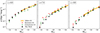 |
Fig. 2. UV luminosity functions (LFs) at 6≤z≤8 from our fiducial model, compared with several observational estimates. We show Hubble estimates from Bouwens et al. (2021) and Finkelstein et al. (2015), as well as the observation-averaged posterior from Gillet et al. (2020) (1σ credible interval). |
 |
Fig. 3. Lyman-α luminosity functions at z = 6.6. Our fiducial model is based on equivalent width distributions of photometrically selected candidates (see text for details). We also show narrow-band selected LAE LFs from Subaru (Umeda et al. 2025). |
2.2.2. Selection with other lines
We also considered spectroscopic confirmation targeting other nebular lines. We used the planned JWST survey as a template: the First Reionization Epoch Spectroscopically Complete Observations (FRESCO; Oesch et al. 2023). FRESCO will target a field of 62 square arcminutes at a depth of mAB∼28.2 using the NIRCam/grism instrument. NIRCam filters are sensitive to Hα below redshift 7 and sensitive to [OIII] and Hβ for z∈(7,9).
We produced separate galaxy maps using the above line selection criterion for various magnitude cutoffs in order to forecast prospects for the 21-cm cross-correlation with FRESCO or a FRESCO-like field. We made the common assumption that the luminosity of these low-opacity nebular lines traces the star formation rate of the galaxy (e.g., Kennicutt 1998; Ly et al. 2007; Gong et al. 2017),
![$$ L_{\mathrm {[OIII]}} =\mathrm {SFR}\times 1.32\cdot 10^{41}\frac {\mathrm {erg}\cdot \mathrm {yr}}{\mathrm {s}\cdot \mathrm {M}_\odot }, $$](/articles/aa/full_html/2025/07/aa54456-25/aa54456-25-eq24.gif)
and
where the SFR is in units of M⊙/yr and the luminosity is in erg/s.
3. Computing the S/N of the cross-power spectrum
After computing the cosmic signals, we determined the detectability of the galaxy–21-cm cross-power spectrum given a specific pair of instruments. We computed the power spectrum in cylindrical coordinates (k⊥,k∥) because this is the natural basis for interferometers that seek to maximize the S/N of a detection. Furthermore, this basis relegates foreground contamination to an easily excised (at least in principle) corner of Fourier space. Here, k⊥ refers to wavemodes in the sky plane, and k∥ refers to wavemodes along the line of sight. Thus, a cylindrical cross-power spectrum was constructed by independently averaging Fourier modes along the line of sight and in sky-plane bins.
We split each lightcone into redshift chunks, each with a frequency-domain depth of Δν = 6 MHz centered on redshift z. From each chunk, we computed the cross-power spectra,

where P21,g(z) is the galaxy–21-cm cross-power spectrum, δTb(z) is the 21-cm brightness temperature field, and  is the galaxy overdensity field.
The averaging in the above equation was computed only over wavemodes that are accessible to a specific instrument or survey and that were not highly contaminated by foregrounds or systematics. Averaging over systematics-contaminated modes might still improve the S/N, because that uncorrelated systematics do not impact the mean of the cross-power, even though they increase the variance (e.g., Fronenberg & Liu 2024). In order to quantify exactly which wavemodes should be excised, however, we would need to forward-model systematics or foreground residuals. We save this for future work and made the simplifying assumption that foreground- or systematics-dominated wavemodes are unusable while the remaining wavemodes include no residual systematics.
We show a schematic of these contaminated or missing regions in 2D Fourier space in Figure 4. Each shaded region illustrates some range of wavemodes that contribute negligibly to the cross-power due to some properties of the instrument/survey/systematics. These include the area of the overlap between the galaxy field and 21-cm field (limited by the galaxy survey footprint), the redshift uncertainty of the galaxies, and contamination by 21-cm foregrounds.
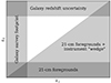 |
Fig. 4. Schematic illustrating regions in the cylindrical power spectrum that contribute negligibly to the cross-power S/N due to instrument, survey, or systematic limitations. |
The galaxy survey will typically have the smaller of the two footprints2, and it can range from tens to hundreds of square degrees for narrow-band dropout or grism surveys to ≲sq. deg for deep follow-up of photometric candidates using high-resolution spectroscopy. The area of the galaxy survey sets the largest on-sky scale (smallest k⊥) accessible for computing the cross-power spectrum. Similarly, the galaxy redshift uncertainty effectively sets the smallest accessible line-of-sight scale (largest k∥; as described further below, we did not excise the larger k∥ modes, but instead accounted for the corresponding uncertainty when we computed the noise). The redshift uncertainty we considered ranged from δz∼0.05 for narrow-band LAE surveys to δz∼0.001 for spectroscopy3 (see Table 2).
21-cm and galaxy survey parameters considered.
Finally, the spectral smoothness of 21-cm foregrounds excludes the lowest k∥ scales. More importantly, the response function of 21-cm interferometers results in leakage of foreground emission into a wedge-shaped region of Fourier space, that overwhelms the cosmic signal (e.g., Datta et al. 2010; Pober et al. 2014; Dillon et al. 2014; Liu et al. 2014a; Pober 2014). To quantify the wedge-contaminated region, we used different slopes in cylindrical k-space (e.g., Thyagarajan et al. 2015),
where Dc(z) is the comoving distance to that redshift, and θFoV is the angular radius of the field of view of the beam of the 21-cm interferometer (see also Munshi et al. 2025 for an alternative characterization of the wedge). We considered three foreground scenarios in this study: a fiducial scenario in which only k-modes up to the slope in Equation (21) are foreground-dominated, a pessimistic scenario in which we doubled the slope, and an optimisic scenario where we halved the slope to represent the recovery of lost Fourier modes via advanced foreground-mitigation techniques (e.g., Hothi et al. 2020; Gagnon-Hartman et al. 2021; Bianco et al. 2024; Kennedy et al. 2024). Foreground scenarios typically vary from horizon-limited to beam-limited, with the former corresponding to our fiducial scenario and the latter to our pessimistic scenario. We also varied the extent of intrinsic foregrounds in each scenario by excising k∥≤0.07 Mpc−1 for the fiducial and optimistic scenarios and k∥≤0.175 Mpc−1 for the pessimistic scenario (Kubota et al. 2018).
After we defined the cross-power spectrum as well as the region in cylindrical Fourier space over which it was computed, we estimated the associated uncertainty. The variance of the cross-power spectrum is (see Lidz et al. 2009)
![$$ \sigma ^2_{21,g}(k_\perp ,k_\parallel ) = {\mathrm {var}}\left [\frac {1}{T_0(z)}P_{21,g}(k_\perp ,k_\parallel )\right ], $$](/articles/aa/full_html/2025/07/aa54456-25/aa54456-25-eq29.gif)
which reduces to
![$$ \sigma ^2_{21,g}(k_\perp ,k_\parallel ) = \frac {1}{2}\left [P^2_{21,g}(k_\perp ,k_\parallel )+\sigma _{21}(k_\perp ,k_\parallel )\sigma _g(k_\perp ,k_\parallel )\right ]. $$](/articles/aa/full_html/2025/07/aa54456-25/aa54456-25-eq30.gif)
Here, T0 is a dimensionless normalization factor defined as
![$$ T_0(z) = 26\left (\frac {T_S-T_\gamma }{T_S}\right )\left (\frac {\Omega _b h^2}{0.022}\right ) \left [\left (\frac {0.143}{\Omega _m h^2}\right )\left (\frac {1+z}{10}\right )\right ]^{1/2}, $$](/articles/aa/full_html/2025/07/aa54456-25/aa54456-25-eq31.gif)
where z is the redshift, TS is the 21-cm spin temperature, Tγ is the CMB temperature, Ωb and Ωm are the baryonic and total matter densities of the Universe, respectively, and h is the dimensionless Hubble parameter.
Similarly to the cross-power, the variance of the auto-power spectra can be written as a sum in quadrature of the cosmic variance and noise power,
![$$ \sigma ^2_{21}(k_\perp ,k_\parallel ) = \frac {1}{2}\left [\frac {1}{T^2_0(z)}P_{21}(k_\perp ,k_\parallel )+P_{21}^{{\mathrm {noise}}}(k_\perp ,k_\parallel )\right ]^2 $$](/articles/aa/full_html/2025/07/aa54456-25/aa54456-25-eq32.gif)
and
![$$ \sigma ^2_{g}(k_\perp ,k_\parallel ) = \frac {1}{2}\left [P_{g}(k_\perp ,k_\parallel )+P_{g}^{{\mathrm {noise}}}(k_\perp ,k_\parallel )\right ]^2, $$](/articles/aa/full_html/2025/07/aa54456-25/aa54456-25-eq33.gif)
where the first terms on the right sides correspond to cosmic variance, while  and
and  correspond to the 21-cm thermal noise and the galaxy redshift uncertainty, respectively. We describe these in turn below.
We computed the 21-cm thermal noise power spectrum,  , using 21cmSense (Pober et al. 2014; Murray et al. 2024). We used antenna layouts corresponding to the full HERA-350 array (Berkhout et al. 2024), as well as the initial AA* deployment of SKA-low (Sridhar 2023). We assumed a 1080 h total integration of drift scan for HERA-350/SKA-low with 6 hours of observation per night over 180 days4. The resulting thermal noise is plotted in Figure 5. Our mock survey with SKA-low resulted in overall lower noise. This is most evident at the largest k⊥, which are better sampled because the SKA-low has a greater number of long core baselines. We also show the three different wedge scenarios we considered with diagonal lines. Optimistic foreground removal would benefit SKA-low far more than HERA-350, since these wedge modes in HERA have very high levels of thermal noise. Foreground-avoidance was indeed a design choice for HERA.
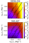 |
Fig. 5. The cylindrical noise power spectra of HERA-350 (top) and SKA-low AA* (bottom) for a fiducial 1000 hour observation at redshift 6.1. The diagonal lines in each panel denote the three choices for wedge excision considered in this work. |
We adopted the galaxy noise model of Lidz et al. (2009), wherein the shot noise sets the minimum noise level and the redshift uncertainty governs the line-of-sight positional uncertainty,
![$$ P^{{\mathrm {noise}}}_g(k_\parallel ) = \frac {1}{n_{{\mathrm {gal}}}}\exp {\left [k_\parallel ^2\left (\frac {c\sigma _z}{H(z)}\right )^2\right ]}, $$](/articles/aa/full_html/2025/07/aa54456-25/aa54456-25-eq37.gif)
where ngal is the number density of galaxies in the survey volume and σz is the redshift uncertainty set by the instrument. This form for  states that the galaxy power spectrum is suppressed by a Gaussian kernel whose width equals the characteristic scale of redshift uncertainties in the field (Seo & Eisenstein 2003). Fisher et al. (1993) and Feldman et al. (1994) showed that this suppression arises naturally in measured galaxy power spectra. As shown in Table 2, we used three fiducial values for σz that corresponded to narrow-band dropouts (LAE; e.g. Ouchi et al. 2018), imaging (i.e., slitless) spectroscopy (grism/prism; e.g. Wang et al. 2022; Oesch et al. 2023), and slit spectroscopy (e.g., Evans et al. 2015; Maiolino et al. 2020).
The signal-to-noise ratio in each bin (k⊥,k∥) depends not only on the cross-power amplitude and uncertainty, but also on the number of Fourier modes sampled by that bin (i.e., sample variance). When the bins are of equal length in log-space, the number of modes per bin is
where Vsurvey is the volume of the survey in comoving units. The signal-to-noise ratio in a single bin adds in quadrature with the number of Fourier modes sampling that bin:
Following Furlanetto & Lidz (2007), we computed the global signal-to-noise ratio as the sum in quadrature of5 the signal-to-noise ratios in each (k⊥,k∥) bin and z,
Figure 6 illustrates the principal data products in our pipeline for estimating the signal-to-noise ratio of the cross-power spectrum. The first two panels from the left show the galaxy and 21-cm auto-power spectra, respectively, as computed from a 1 Gpc coeval cube at z = 6.1. The third panel shows the galaxy–21-cm cross-power spectrum of the same cube. The correlation between the k-modes is weaker than in the galaxy or 21-cm spectra. The rightmost panel shows the resulting signal-to-noise ratio from Equation (29). Superimposed on each panel are shaded regions corresponding to wavemodes that are inaccessible due to survey/instrument/systematics limitations. The final S/N primarily depends on the unshaded wavemodes in the rightmost panel, which are extended to also include other redshift bins.
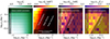 |
Fig. 6. Power spectra of the galaxy field, 21-cm brightness temperature field, their cross-power spectrum, and the signal-to-noise ratio of the cross-power spectrum as a function of k∥ and k⊥ for a fiducial scenario (left to right). Overlaid are various noise-dominated/excluded regions imposed by systematics and observational effects. The 21-cm brightness temperature power spectrum includes cuts showing the three foreground + instrument (i.e. wedge) contamination scenarios we considered. In this illustrative example, the galaxy survey footprint corresponds to ∼1 sq. deg. at z∼6, and the galaxy redshift uncertainty corresponds to δz∼0.01, which is characteristic of slitless spectroscopy. |
4. Mock observations
The galaxy–21-cm cross-power depends on the telescopes used for each observation as well as on the survey strategies. As discussed above, our fiducial 21-cm observations are 1080 h total integration with either HERA-350 or SKA-low AA*. For simplicity, we did not vary the 21-cm survey specifications.
We considered three general types of instruments that are used for galaxy surveys, in order of increasing redshift accuracy6:
-
Narrow-band dropout uses narrow photometric bands to identify Lyman-α line emission. Galaxies thus identified are commonly referred to as LAEs, and their associated redshift uncertainty is determined by the photometric bands used in the drop-out selection. We took Subaru as a fiducial telescope, assuming a redshift uncertainty of 5% (Ouchi et al. 2018).
-
Imaging (slitless) spectroscopy by slitless spectrographs (e.g., grism) provides low-resolution multiple spectra within a contiguous field, without requiring a preselection of candidates through broad-band photometry. We took Roman as our fiducial telescope for LAE-selected surveys and JWST (NIRCam) for Hα/Hβ/OIII-selected surveys. We assumed a redshift uncertainty of 1% for the two instruments (Wang et al. 2022).
-
Slit spectroscopy of high resolution spectrographs result in the smallest redshift uncertainty. Slit spectroscopy requires follow-up of photometric candidates, however, either from existing fields or from new fields. We assumed that photometric candidates of sufficient depth are available (e.g., Euclid Deep Field South Euclid Collaboration: McPartland et al. 2025, SILVERRUSH Ouchi et al. 2018, legacy Hubble fields), and the bottleneck comes from the spectroscopic follow-up of Lyman-α. We adopted a slit spectroscopy redshift uncertainty of 0.1% (e.g., Maiolino et al. 2020).
For each pair of galaxy–21-cm instruments, we computed the S/N of the cross-power as a function of the galaxy survey area and AB magnitude limit in the relevant observing band, which is denoted as  for Ly-α selected surveys and mAB for Hα/OIII selected surveys. Figure 7 illustrates the stochastic relation between intrinsic galaxy parameters and Ly-α emission, showing that the UV continuum magnitude of a galaxy MUV does not uniquely determine its
  . We superimpose horizontal lines corresponding to the Ly-α band limiting AB magnitudes of the MOONRISE and Roman HLS surveys (Maiolino et al. 2020; Wang et al. 2022). Slit-spectroscopic galaxy surveys require a photometric candidate survey, complete down to some MUV, on which they perform follow-up observations. We did not investigate the effect of MUV incompleteness of the photometric candidates on the assumption that a candidate survey is deep enough for a slit-spectroscopic follow-up survey of a given
  limit to be performed with full completeness. For example, a Lyman-α spectroscopic survey at z∼7 with a depth of
  would require follow-up of photometrically selected candidates down to MUV≤−20 in order to be ≥95% complete (see Fig. 7).
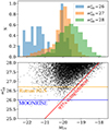 |
Fig. 7. Distribution of UV continuum magnitudes (MUV) and Lyman-α band AB magnitudes ( |


We produced six realizations of each observed galaxy field for magnitude cuts ranging from  to
to  and averaged the S/N at each magnitude cut. In our calculation of band magnitude, we assumed that the relevant band is dominated by line emission, which is reasonable because only LAEs with equivalent width greater than unity are detectable at the considered magnitude cuts. The total S/N of the cross-power spectrum varies fairly smoothly between magnitude cuts, so we devised an analytic form for S/N as a function of magnitude cut for each galaxy selection criterion, described in Appendix C. Moreover, the S/N varied trivially with the survey angular area and required only a cut in cylindrical Fourier space as well as the noise rescaling introduced in Equation (28). The redshift uncertainty is likewise easy to implement via Equation (27).
Although our predictions for the cross-spectrum S/N can be used to design new surveys, we used existing/proposed surveys as a reference. These are listed in Table 3. Of these, SILVERRUSH is already underway, and FRESCO, MOONRISE, and HLS are scheduled for execution in the coming years. We also consider a prospective spectroscopic follow-up survey using ELT MOSAIC modeled after MOONRISE.
Benchmark galaxy surveys.
The Systematic Identification of LAEs for Visible Exploration and Reionization Research Using Subaru HSC (SILVERRUSH) survey is a long-running program for the identification of tens of thousands of LAEs via narrow-band dropout covering redshifts 2−7 (Ouchi et al. 2018). The survey area of SILVERRUSH ranges from 13.8 square degrees at z∼5.7–21.2 square degrees at z∼6.6 (Umeda et al. 2025). To split the difference between these survey footprints while producing the same number of galaxies, we took our SILVERRUSH benchmark to cover an equal 16 square degrees at all redshifts and to observe down to  . The limiting factor when computing the S/N of the cross-power using SILVERRUSH is its narrow-band dropout strategy, which results in a relatively large redshift uncertainty. Many of these LAE are being followed up with spectroscopy, however, which should reduce these errors in the future.
The Nancy Grace Roman Space Telescope will conduct a High Latitude Survey (HLS) over a huge swathe of sky covering ∼2000 sq. deg. using its near-IR grism. Of this, 500 sq. deg. overlap with the HERA stripe, and to facilitate the comparison between cross-correlation forecasts with SKA-low AA* and HERA-350, we limited the effective survey footprint of the Roman HLS to 500 sq. deg.. Based on ∼0.6 years of observing time, the survey is expected to detect tens of thousands of z>5 galaxies via the Lyman-break technique. The frequency range of the near-IR band means that Roman can only detect Lyman-α emission at z>7.2 (Wang et al. 2022). La Plante et al. (2023) forecast the significance of a cross-power spectrum detection made using a Lyman-α survey from Roman and a 21-cm field measured using HERA. We confirm their findings and extend them to an SKA-low AA* measurement of the 21-cm signal. Although HLS benefits from a large sky area, its imaging spectroscopy is limited to z>7.2, which significantly limits the S/N compared to surveys extending to lower redshifts. The LBG sample from Roman might be followed-up with slit spectroscopy (with, e.g. MOSAIC on the ELT), however, which would provide galaxy maps throughout the EoR.
The First Reionization Epoch Spectroscopically Complete Observations (FRESCO) survey is a Cycle 1 medium program slated for execution on the James Webb Space Telescope (Oesch et al. 2023). FRESCO will cover 62 square arcminutes and observe out to a depth of mAB≈28.2 using NIRCam/grism. FRESCO targets Hα at z<7 and [OIII] and Hβ for z∈(7,9). Although its target area is much smaller than that of the other benchmark surveys, FRESCO observes to much deeper magnitudes and selects on low-opacity emission lines. This allows a more accurate redshift determination (for simplicity, we used the same redshift uncertainty for all slitless surveys).
The MOONS Redshift-Intensive Survey Experiment (MOONRISE) is a guaranteed observing time program of the MOONS instrument, a powerful spectrometer scheduled for deployment at the Very Large Telescope (VLT) (Maiolino et al. 2020). MOONRISE will spectroscopically follow up ∼1100 candidate LAEs down to  in a ∼1 square degree field at z>5. MOONRISE walks the middle path of reasonable survey area, moderate survey depth, and good redshift uncertainties, making it a promising candidate among slit spectroscopy surveys for cross-correlation with 21-cm.
Finally, we provide forecasts using a prospective survey on the next-generation multiplex spectrograph ELT MOSAIC, which is currently in development for deployment at the Extremely Large Telescope (ELT). We provide forecasts for MOONRISE-like surveys performed using ELT MOSAIC assuming an  5σ 5-hour limiting magnitude (Evans et al. 2015; Kehrig, private communication).
5. Results
Before presenting our main results of the S/N forecasts, we briefly review the general behavior of the cross-power spectrum and the information it contains. Figure 8 shows the galaxy–21-cm cross correlation coefficients (CCCs) at z∈(6.2,7.0,8.0,9.0) for our fiducial model. The CCCs are defined as
where P21,g(k), P21(k), and Pg(k) are the 1D galaxy–21-cm cross-, 21-cm auto-, and galaxy auto-power spectra, respectively. With this normalization, the CCCs provide a clean measure of the phase difference between the two fields: CCC →0 for uncorrelated fields, CCC →1 for correlated fields, and CCC →−1 for anti-correlated fields (e.g., Lidz et al. 2009; Sobacchi et al. 2016; Fronenberg & Liu 2024). The top and bottom panels correspond to different Ly-α magnitude cuts. One cut is ambitiously deep ( ; cf. Table 3) and another cut is even deeper in order to show physical trends (
 ).
).
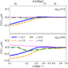 |
Fig. 8. Galaxy–21-cm correlation coefficients at z∈(6.2,7.0,8.0,9.0), assuming at two Ly-α magnitude cuts: |


We recovered the qualitative trends noted in previous studies on the cross-power and the CCCs (e.g., Furlanetto & Lidz 2007; Lidz et al. 2009; Sobacchi et al. 2016; Hutter et al. 2023; La Plante et al. 2023). The CCCs tend toward zero on small scales during the EoR (z≲8) and the preceding EoH (z≳8; see Figure 1) because the relative locations of galaxies inside either ionized HII bubbles or heated IGM patches do not impact the cross-power, and thus the two fields on those small scales could have random phases (e.g., Lidz et al. 2009; Sobacchi et al. 2016; Fronenberg & Liu 2024). On the other hand, because the galaxies and 21-cm both depend on the large-scale matter field, the CCCs on large scales tend to either −1 or 1, during the EoR and EoH, respectively (e.g., Heneka & Mesinger 2020). The transition of the CCCs from 0 to 1 (−1) encodes the typical sizes of heated (ionized) IGM patches during the EoH (EoR; see Sobacchi et al. 2016; Heneka & Mesinger 2020; Moriwaki et al. 2024).
However, the asymptotic trend of the CCC to 1 or −1 on large scales is only reached in the limit of an infinite galaxy survey depth, which would effectively measure the DM halo–21cm cross-correlation (see Fig. 3 in Sobacchi et al. 2016). Realistic magnitude cuts together with the intrinsic stochasticity in the galaxy – halo connection discussed in the previous section, result in a much smaller large-scale (anti)correlation of the galaxy and 21 cm fields. For  in the top panel of Fig. 8, the CCCs only reach −0.5 during the EoR, while no signal is detected during the EoH at z>8 (see also Fig. 14). For
  in the bottom panel, the large-scale CCC trends are closer to the theoretically expected limiting cases, and even the positive correlation during the EoH can be seen at z = 9. However, depths of
  on reasonably sized fields would require over 10 k hours of integration with slit spectroscopy, as we describe below.
In Figures 9 –13 we show the main results of this work: The expected S/N for every survey configuration considered in this study. Each figure shows the S/N of the galaxy–21-cm cross-power spectrum as a function of observing depth and survey footprint, for narrow-band dropout, slitless and slit spectroscopy (left to right panels). Different figures vary the 21-cm instrument (HERA-350 vs. SKA-low AA*) as well as the level of 21-cm wedge contamination (optimistic, fiducial, pessimistic). In the spectroscopy panels for Lyα-selected galaxy surveys, we show 100- and 1000-hour isochrones for observations using the ELT MOSAIC instrument. These isochrones correspond to the total observation time, equal to the number of 40 sq. arcmin pointings required to reach the desired survey footprint on the vertical axis, times the exposure time per pointing required for a ≥5σ detection down to the given limiting  on the horizontal axis (using the latest MOS-NIR-LR sensitivity estimates; Kehrig, private communication).
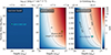 |
Fig. 9. Effect of observing depth, field of view, and galaxy survey type on the signal-to-noise ratio of a cross-power spectrum detection. Each panel corresponds to a different galaxy survey type, which determines the mean redshift uncertainty associated with that survey. On the top axis of the slit spectroscopy panel, we show the corresponding rest frame UV magnitude limit required for ≥2σ completeness of the photometric candidate sample (see Fig. 7). Blue stars correspond to the SILVERRUSH and MOONRISE high-redshift galaxy surveys, and the orange star corresponds to an overlap of the Roman HLS survey and a single SKA-low AA* beam; multiple 21-cm fields can be tiled to increase the S/N in quadrature as discussed in the text. The MOONRISE spectroscopic survey should enable a 3σ detection of the cross-spectrum. In the spectroscopy panel we also show 100- and 1000-hour isochrones for potential future surveys using MOSAIC on the ELT. |
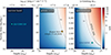 |
Fig. 10. As Figure 9, but assuming the pessimistic foregrounds shown in Figure 6. Here, MOONRISE is no longer sufficient for a 3σ cross-spectrum detection, but a 1000-hour survey with MOSAIC remains viable. |
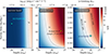 |
Fig. 11. As Figure 9, but assuming the optimistic foreground scenario in Figure 6. SILVERRUSH remains not viable, although an extremely deep survey of similar angular extent could theoretically breach 3σ, and the S/N with spectroscopy improves only slightly. |
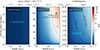 |
Fig. 12. As Figure 9, but using HERA rather than the SKA-low as the fiducial 21-cm interferometer. Notably, the lack of sensitivity of HERA to high k⊥ modes (i.e. small sky plane scales) precludes detection of the cross-spectrum using a galaxy field with a small (∼5 sq. deg.) field of view. Wide-area slitless spectroscopy remains the only viable candidate for cross-correlating galaxy maps with HERA 21-cm data. |
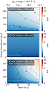 |
Fig. 13. Effect of observing depth and field of view on a FRESCO-like survey that selects for Hα at z<7 and [OIII]/Hβ at z≥7. The FRESCO 62 square arcminute fields are too small to yield a detection of the 21-cm cross-power spectrum. |
An increased redshift uncertainty suppresses S/N exponentially, which requires an exponential rise in the number of galaxies that are detected to compensate. This may be achieved by either dramatically increasing the survey footprint or increasing the observing depth by a few magnitudes. Therefore, we evaluated the S/N of narrow-band dropout and grism surveys on a wider range of footprint sizes and a deeper range of observing depths than the slit spectroscopic surveys. Furthermore, we limited the sensitivity of the grism surveys in this experiment to z>7.2 to reflect the grism filter of the Nancy Grace Roman Space Telescope.
When the surveys are deeper than  , the S/N increases more readily with survey area than with the observing depth in all cases. For spectroscopic surveys, we find that targeting a depth of
  and maximizing the contiguous survey footprint yields the highest S/N per unit survey time.
In our fiducial model,  corresponds to the observing depth at which the maximum value of the galaxy power spectrum Pgal(k) roughly equals the noise power 1/ngal (ignoring redshift uncertainty), and therefore, the S/N of the galaxy auto-power spectrum at this depth for a single field is ∼1. This is consistent with the recommendation of Tegmark (1997) to extend the depth of a single field until the S/N reaches 1 and then tile additional fields to time-efficiently maximize the total S/N. We discuss this result in greater detail in Appendix C.
5.1. SKA–Lyman Alpha
Figure 9 shows our results for a Lyman-α galaxy survey paired with an SKA-low AA* 21-cm measurement assuming the fiducial foreground scenario. The left panel shows that the SILVERRUSH sample without a spectroscopic follow-up is insufficient for a cross-power detection. This contradicts some previous claims (e.g., Sobacchi et al. 2016; Hutter et al. 2018), which treated the redshift uncertainties in the LAE sample more simplistically. Even an extremely deep narrow-band dropout survey (i.e.,  ) of a similar area cannot yield a significant cross-spectrum detection, except in the case of optimistic 21-cm foreground recovery. This highlights the importance of small redshift uncertainties in measuring the cross-power spectrum.
The middle panel includes a forecast for Roman HLS using a survey footprint equivalent to the beam size of SKA-low AA*. The enormous angular survey extent of Roman means that in this case alone, the footprint for the cross-correlation is limited by the field of view of the 21-cm instrument. We find that a single patch of the SKA-low AA* beam within Roman HLS yields an 8σ detection of the cross-power spectrum. Tiling multiple beams can increase the S/N. For example, 47 patches of the SKA-low AA* beam can fit within 500 sq. deg. of overlapping area, which would bring the cumulative S/N from to  .
.
The right panel shows that the planned MOONRISE survey should be sufficient to measure the cross-power spectrum at a ∼3σ significance. Furthermore, the dashed contours delineating prospective MOSAIC configurations imply that a similar survey using MOSAIC could achieve a ∼4σ measurement of the cross-power spectrum in ∼500 hours of observation targeting ∼1–3 sq. deg. An extension of this to 1000 h can bring the S/N up to 5σ.
Figures 10 and 11 show our results for the same Lyman-α galaxy survey and SKA-low observations, but assuming pessimistic and optimistic 21-cm foregrounds, respectively. Figure 10 shows that the significance of a cross-spectrum measurement depends very strongly on the level of the foregrounds and that our strong foreground case precludes a detection of the cross-power spectrum using the MOONRISE survey. However, a 1000-hour observation using ELT MOSAIC could yield a ∼3σ detection. We find that an increase in the number of telescope pointings (assuming equal exposure time per pointing) yields more S/N per unit observing time than boosting exposure depth. Figure 11 shows that when a significant portion of 21-cm foreground wedge modes is recovered, the narrow band dropout redshift uncertainty still precludes a cross-spectrum measurement for the range of survey configurations we considered.
5.2. HERA–Lyman-alpha
Figure 12 shows our results for a Lyman-α galaxy survey paired with a measurement of the 21-cm signal made using HERA-350. Compared with SKA-low, the lack of sensitivity of HERA to high k⊥ modes precludes cross-spectrum detections using galaxy fields with small angular footprints. This is evident in the rightmost panel of Figure 12, where neither MOONRISE nor MOSAIC can yield a cross-spectrum detection with HERA.
The most promising candidate for a cross-correlation with HERA are large-area surveys with slitless spectroscopy, shown in the middle panel using the benchmark HLS with Roman grism. The star in this panel shows the forecast from La Plante et al. (2023), which we match to within 10%7. We predict a ≳6σ detection of the cross-power for a Roman HLS + HERA-350 observation in a single HERA beam covering 100 sq. deg. Since HERA always operates in drift-scan mode, it will observe a cumulative five patches of this size in the Roman HLS field, which means a total of S/N  for the full 500 sq. deg. of overlap. This is very close to the S/N = 14 quoted by La Plante et al. (2023).
5.3. SKA–OIII/H Alpha
Figure 13 shows our results for a NIRCam-like galaxy survey targeting Hα below z = 7 and [OIII]/Hβ for z∈(7,9) paired with a 21-cm signal measured by the SKA-low. The two bottom panels show S/N forecasts for a cross-correlation using SKA-low AA*, and the top panel uses SKA-low in its planned AA4 upgraded configuration, which includes additional outrigger antennas (Sridhar 2023). The two top panels assume fiducial foregrounds, and the bottom panel uses optimistic foregrounds. Fiducial foregrounds preclude a detection of the galaxy–21-cm cross-power spectrum in a FRESCO-like survey paired with SKA-low AA*. Even when we invoke AA4 or optimistic foregrounds, the FRESCO footprint remains too small to claim a cross-spectrum detection. However, a FRESCO-like survey with the same observing depth but ten times the survey footprint would yield a ∼3σ detection of the 21-cm signal in cross-correlation using SKA-low AA4. This is not far-fetched because FRESCO itself is only a 53-hour program and produces two noncontiguous pencil beams. Using the same exposure time per pointing, it would only take ∼240 hours to expand a single FRESCO beam into a field that is large enough for cross-correlation.
5.4. Redshifts that contribute to the signal-to-noise ratio
We also investigated which redshift bins contribute the most to the total S/N. We show the cumulative S/N for fiducial galaxy surveys using MOSAIC, Roman, and JWST (with FRESCO-like selection) as a function of redshift (bottom axis) and IGM neutral fraction (top axis) in Figure 14. The lowest-redshift bins with nonzero neutral hydrogen dominate the S/N of all surveys we considered. This reflects the fact that any magnitude-limited survey detects significantly more galaxies at low redshift than at high redshift. This effect is most pronounced for Ly-α selected surveys because the sensitivity of Lyα to IGM attenuation increases the cross-power during the EoR while making it more difficult to detect galaxies pre-EoR. Galaxy surveys targeting nebular lines with low IGM opacities, such as FRESCO, result in an S/N that is distributed over a broader range in redshift. The plateau in the cumulative S/N at z∼8–9 is caused by the equality between the 21-cm spin temperature and the CMB temperature at this redshift in our fiducial model, which drives a sign change in the cross-power (see Figure 8 and associated discussion).
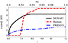 |
Fig. 14. Cumulative S/N of the galaxy–21-cm cross-power spectrum as a function of redshift for fiducial observations using MOSAIC, JWST, and Roman. The MOSAIC observation corresponds to our recommended ELT survey, the Roman observation corresponds to and integration over two patches of the SKA-low field of view within the Roman observing area, and the JWST observation corresponds to the FRESCO survey. The Roman and MOSAIC surveys are Ly-α selected, so that redshifts higher than ∼8 contribute negligibly to their total S/N due to attenuation from the neutral IGM. On the other hand, FRESCO selects on Hα and [OIII], allowing higher-redshift galaxies to contribute to the total S/N. The global neutral IGM fraction is indicated on the upper horizontal axis. |
6. Conclusion
A detection of the cosmic 21-cm signal would usher in a new era for research on the Epoch of Reionization (EoR). Radio interferometers aim to make a preliminary detection of the power spectrum with a low signal-to-noise (S/N) in the coming years. A cross-correlation of the preliminary signal with galaxies will provide a crucial sanity check for initial 21-cm detection claims because the tracer systematics are uncorrelated.
We forecast the S/N of the cross-power in various pairings of prospective galaxy surveys and 21-cm interferometers. Our fiducial 21-cm observations used 1000-hour integrations of the SKA-low AA* and HERA-350 instruments. These were paired with galaxy surveys of varying survey area, depth, and selection method (narrow-band, slitless spectroscopy, and slit spectroscopy) to compute the galaxy–21-cm cross-power spectrum and quote an S/N for each scenario. We also varied the level of 21-cm foreground contamination that would be excised before computing the cross-power.
To compute mock observations, we self-consistently simulated large (1 Gpc) galaxy and 21-cm fields using 21cmFASTv4 (Davies et al. 2025). We then post-processed the galaxy field to include only galaxies whose line luminosities in a given band (spanning either Lyman-α or Hα/Hβ/OIII) exceeded the sensitivity threshold for the survey of interest. To connect the line luminosities to the galaxy UV continuum magnitude or star formation rate, we sampled empirical relations provided by Mason et al. (2018) for Ly-α and Gong et al. (2017) for other lines.
Our mock galaxy surveys were set up for an easy comparison with benchmark instruments, including Subaru HyperSupremeCam, Roman grism, VLT MOONS, ELT MOSAIC, and JWST NIRCam. Our principal results are listed below.
-
Even pessimistic 21-cm foregrounds do not preclude a detection of the cross-power with galaxies when the slitless spectroscopic survey area is very large or the slit spectroscopic survey is very deep. Overall, the different foreground contamination scenarios we studied affect the achievable S/N by factors of few.
-
Narrow-band dropout surveys are unlikely to detect the cross-power spectrum due to their poor redshift localization.
-
Large-field slitless spectroscopy with Roman grism yields the highest S/N cross-power detection: ∼55σ (∼13σ) paired with SKA-low AA* (HERA-350), for our fiducial model and assuming ∼500 sq. deg. of overlap. Although the Roman grism is only sensitive to Ly-α at z≥7.2, the Roman redshift precision and huge observing area more than compensate for the loss in signal from the missing lower-redshift galaxies.
-
Small-field slitless spectroscopy targeting Hα/HβOIII using JWST NIRCam, as per the FRESCO survey (Oesch et al. 2023), does not yield a high enough S/N for a detection of the cross-power spectrum. However, a survey of similar depth that covers about ten times the area would yield a ∼3σ detection of the 21-cm signal in cross-correlation with a 21-cm measurement provided by a planned upgrade of SKA: AA4.
-
Slit spectroscopy can provide high S/N cross-power for SKA-low AA* observations. Specifically, the planned MOONRISE survey with VLT MOONS can result in a ∼3σ detection (Maiolino et al. 2020). We likewise showed that a 4σ detection can be made with ELT MOSAIC for a comparable observation time for a survey with area ∼1–3 sq. deg. (Evans et al. 2015).
These forecasts are intended as a guide for future survey strategies to facilitate the detection of the galaxy–21-cm cross-power spectrum.
Acknowledgments
We thank S. Murray for helpful guidance regarding the generation of noise for the 21-cm field. Additional thanks to D. Breitman for providing a handy script for rapid power spectrum calculations. We extend further gratitude to S. Carniani, L. Pentericci, and M. Hayes for useful discussions regarding upcoming surveys, as well as to A. C. Liu for invaluable feedback on a draft version of this paper. We gratefully acknowledge computational resources of the HPC center at SNS. AM acknowledges support from the Italian Ministry of Universities and Research (MUR) through the PRIN project “Optimal inference from radio images of the epoch of reionization”, and the PNRR project “Centro Nazionale di Ricerca in High Performance Computing, Big Data e Quantum Computing”.
In principle, the redshift uncertainty is determined by a combination of instrument resolution, peculiar velocity, and the offset of the Lyman-α line from systemic. The latter two effects set a lower limit for the achievable redshift uncertainty, which is about δz∼0.001. We postpone a more careful treatment of each of these terms to future work focusing on specific instruments.
The SKA-low AA* beam covers a stripe on the sky with a width of 3.68°. Integrating for 6 hours per night over the same stripe produces a survey footprint of 332 sq. deg.. Similarly, HERA covers a stripe of width 11.0° and thus produces a survey footprint of 990 sq. deg. (Murray et al. 2024). We assume Gaussian beams, and the widths quoted above correspond to the 3σ extents.
Our choice to treat the global S/N as the quadrature sum of the S/N in each bin reflects our assumption that the noise in each Fourier mode is statistically independent. This assumption results in a modest overestimation of the signal-to-noise ratio (e.g., Liu et al. 2014a, b, Prelogović & Mesinger 2023).
As mentioned above, we do not consider broad-band photometry (i.e. Lyman break galaxy surveys), because the corresponding redshift uncertainties are too large to be useful for cross correlation with 21-cm (e.g., La Plante et al. 2023).
It is curious, given our different methods, that we match the predicted S/N of a HERA-Roman survey so closely. Relative to the model of La Plante et al. (2023), we produce a lower number density of highly luminous Ly-α-emitting galaxies, and we therefore expect a lower S/N in the galaxy power spectrum for equal observing depth. However, our 21-cm noise model, 21cmSense, differs from the analytic model of La Plante et al. (2023) in that it accounts for baseline rotation during the observation, lowering the noise level in certain k-bins relative to the analytic model. In both cases, the deviations between our model and that of La Plante et al. (2023) are ∼20%, and they conspire to offset each other such that our estimated S/N matches their model within ∼10%.
References
- Adachi, S., Adkins, T., Aguilar Faúndez, M. A. O., et al. 2022, ApJ, 931, 101 [CrossRef] [Google Scholar]
- Adi, T., Flitter, J., & Kovetz, E. D. 2025, Phys. Rev. D, 111, 043515 [Google Scholar]
- Amiri, M., Bandura, K., Chakraborty, A., et al. 2024, ApJ, 963, 23 [Google Scholar]
- Anderson, C. J., Luciw, N. J., Li, Y. C., et al. 2018, MNRAS, 476, 3382 [NASA ADS] [CrossRef] [Google Scholar]
- Barrow, K. S. S., Wise, J. H., Norman, M. L., O’Shea, B. W., & Xu, H. 2017, MNRAS, 469, 4863 [Google Scholar]
- Berkhout, L. M., Jacobs, D. C., Abdurashidova, Z., et al. 2024, PASP, 136, 045002 [Google Scholar]
- Bianco, M., Giri, S. K., Prelogović, D., et al. 2024, MNRAS, 528, 5212 [Google Scholar]
- Bird, S., Ni, Y., Di Matteo, T., et al. 2022, MNRAS, 512, 3703 [NASA ADS] [CrossRef] [Google Scholar]
- Bouwens, R. J., Illingworth, G. D., Oesch, P. A., et al. 2014, ApJ, 793, 115 [Google Scholar]
- Bouwens, R. J., Illingworth, G. D., Oesch, P. A., et al. 2015, ApJ, 811, 140 [NASA ADS] [CrossRef] [Google Scholar]
- Bouwens, R. J., Oesch, P. A., Stefanon, M., et al. 2021, AJ, 162, 47 [NASA ADS] [CrossRef] [Google Scholar]
- Ceverino, D., Klessen, R. S., & Glover, S. C. O. 2018, MNRAS, 480, 4842 [NASA ADS] [Google Scholar]
- Chakraborty, A., & Choudhury, T. R. 2024, JCAP, 2024, 078 [Google Scholar]
- CHIME Collaboration (Amiri, M., et al.) 2023, ApJ, 947, 16 [NASA ADS] [CrossRef] [Google Scholar]
- Clark, S. J., Dutta, B., Gao, Y., Ma, Y. -Z., & Strigari, L. E. 2018, Phys. Rev. D, 98, 043006 [Google Scholar]
- Cooray, A., Bock, J., Burgarella, D., et al. 2016, ArXiv e-prints [arXiv:1602.05178] [Google Scholar]
- Crites, A. T., Bock, J. J., Bradford, C. M., et al. 2014, in Millimeter, Submillimeter, and Far-Infrared Detectors and Instrumentation for Astronomy VII, eds. W. S. Holland, & J. Zmuidzinas, SPIE Conf. Ser., 9153, 91531W [NASA ADS] [CrossRef] [Google Scholar]
- Cunnington, S., Li, Y., Santos, M. G., et al. 2023, MNRAS, 518, 6262 [Google Scholar]
- Curti, M., Mannucci, F., Cresci, G., & Maiolino, R. 2020, MNRAS, 491, 944 [Google Scholar]
- Datta, A., Bowman, J. D., & Carilli, C. L. 2010, ApJ, 724, 526 [NASA ADS] [CrossRef] [Google Scholar]
- Davies, J. E., Bird, S., Mutch, S., et al. 2023, MNRAS, 525, 2553 [NASA ADS] [CrossRef] [Google Scholar]
- Davies, J. E., Mesinger, A., & Murray, S. 2025, A&A, submitted [arXiv:2504.17254] [Google Scholar]
- De Barros, S., Pentericci, L., Vanzella, E., et al. 2017, A&A, 608, A123 [NASA ADS] [CrossRef] [EDP Sciences] [Google Scholar]
- Dillon, J. S., Liu, A., Williams, C. L., et al. 2014, Phys. Rev. D, 89, 023002 [NASA ADS] [CrossRef] [Google Scholar]
- Euclid Collaboration (McPartland, C. J. R., et al.) 2025, A&A, 695, A259 [Google Scholar]
- Evans, C., Puech, M., Afonso, J., et al. 2015, ArXiv e-prints [arXiv:1501.04726] [Google Scholar]
- Facchinetti, G., Lopez-Honorez, L., Qin, Y., & Mesinger, A. 2024, JCAP, 2024, 005 [Google Scholar]
- Feldman, H. A., Kaiser, N., & Peacock, J. A. 1994, ApJ, 426, 23 [Google Scholar]
- Finkelstein, S. L., Ryan, R. E. Jr., Papovich, C., et al. 2015, ApJ, 810, 71 [NASA ADS] [CrossRef] [Google Scholar]
- Fisher, K. B., Davis, M., Strauss, M. A., Yahil, A., & Huchra, J. P. 1993, ApJ, 402, 42 [Google Scholar]
- Fragos, T., Lehmer, B. D., Naoz, S., Zezas, A., & Basu-Zych, A. 2013, ApJ, 776, L31 [CrossRef] [Google Scholar]
- Fronenberg, H., & Liu, A. 2024, ApJ, 975, 222 [Google Scholar]
- Furlanetto, S. R., & Lidz, A. 2007, ApJ, 660, 1030 [Google Scholar]
- Furlanetto, S. R., Zaldarriaga, M., & Hernquist, L. 2004, ApJ, 613, 1 [NASA ADS] [CrossRef] [Google Scholar]
- Furlanetto, S. R., Oh, S. P., & Briggs, F. H. 2006, Phys. Rep., 433, 181 [Google Scholar]
- Gagnon-Hartman, S., Cui, Y., Liu, A., & Ravanbakhsh, S. 2021, MNRAS, 504, 4716 [NASA ADS] [CrossRef] [Google Scholar]
- Gillet, N. J. F., Mesinger, A., & Park, J. 2020, MNRAS, 491, 1980 [NASA ADS] [Google Scholar]
- Gong, Y., Cooray, A., Silva, M. B., et al. 2017, ApJ, 835, 273 [NASA ADS] [CrossRef] [Google Scholar]
- Grazian, A., Giallongo, E., Paris, D., et al. 2017, A&A, 602, A18 [NASA ADS] [CrossRef] [EDP Sciences] [Google Scholar]
- Gunn, J. E., & Peterson, B. A. 1965, ApJ, 142, 1633 [Google Scholar]
- Heneka, C., & Cooray, A. 2021, MNRAS, 506, 1573 [Google Scholar]
- Heneka, C., & Mesinger, A. 2020, MNRAS, 496, 581 [NASA ADS] [CrossRef] [Google Scholar]
- Hothi, I., Chapman, E., Pritchard, J. R., et al. 2020, MNRAS, 500, 2264 [CrossRef] [Google Scholar]
- Hutter, A., Dayal, P., Müller, V., & Trott, C. M. 2017, ApJ, 836, 176 [Google Scholar]
- Hutter, A., Trott, C. M., & Dayal, P. 2018, MNRAS, 479, L129 [Google Scholar]
- Hutter, A., Heneka, C., Dayal, P., et al. 2023, MNRAS, 525, 1664 [Google Scholar]
- Izotov, Y. I., Schaerer, D., Thuan, T. X., et al. 2016, MNRAS, 461, 3683 [Google Scholar]
- Kennedy, J., Carr, J. C., Gagnon-Hartman, S., et al. 2024, MNRAS, 529, 3684 [Google Scholar]
- Kennicutt, R. C. Jr. 1998, ARA&A, 36, 189 [NASA ADS] [CrossRef] [Google Scholar]
- Kern, N. S., Parsons, A. R., Dillon, J. S., et al. 2020, ApJ, 888, 70 [NASA ADS] [CrossRef] [Google Scholar]
- Kimm, T., Cen, R., Devriendt, J., Dubois, Y., & Slyz, A. 2015, MNRAS, 451, 2900 [CrossRef] [Google Scholar]
- Kostyuk, I., Ciardi, B., & Ferrara, A. 2025, A&A, 695, A32 [NASA ADS] [CrossRef] [EDP Sciences] [Google Scholar]
- Kovetz, E. D., Viero, M. P., Lidz, A., et al. 2017, ArXiv e-prints [arXiv:1709.09066] [Google Scholar]
- Kubota, K., Yoshiura, S., Takahashi, K., et al. 2018, MNRAS, 479, 2754 [Google Scholar]
- Kubota, K., Inoue, A. K., Hasegawa, K., & Takahashi, K. 2020, MNRAS, 494, 3131 [Google Scholar]
- La Plante, P., Sipple, J., & Lidz, A. 2022, ApJ, 928, 162 [NASA ADS] [CrossRef] [Google Scholar]
- La Plante, P., Mirocha, J., Gorce, A., Lidz, A., & Parsons, A. 2023, ApJ, 944, 59 [Google Scholar]
- Lehmer, B. D., Eufrasio, R. T., Tzanavaris, P., et al. 2019, ApJS, 243, 3 [NASA ADS] [CrossRef] [Google Scholar]
- Lidz, A., Zahn, O., Furlanetto, S. R., et al. 2009, ApJ, 690, 252 [NASA ADS] [CrossRef] [Google Scholar]
- Liu, A., & Shaw, J. R. 2020, PASP, 132, 062001 [NASA ADS] [CrossRef] [Google Scholar]
- Liu, A., Parsons, A. R., & Trott, C. M. 2014a, Phys. Rev. D, 90, 023018 [NASA ADS] [CrossRef] [Google Scholar]
- Liu, A., Parsons, A. R., & Trott, C. M. 2014b, Phys. Rev. D, 90, 023019 [NASA ADS] [CrossRef] [Google Scholar]
- Ly, C., Malkan, M. A., Kashikawa, N., et al. 2007, ApJ, 657, 738 [NASA ADS] [CrossRef] [Google Scholar]
- Ma, Q., Helgason, K., Komatsu, E., Ciardi, B., & Ferrara, A. 2018, MNRAS, 476, 4025 [NASA ADS] [CrossRef] [Google Scholar]
- Maiolino, R., Cirasuolo, M., Afonso, J., et al. 2020, Messenger, 180, 24 [Google Scholar]
- Mao, X. -C. 2014, ApJ, 790, 148 [Google Scholar]
- Mason, C. A., Treu, T., Dijkstra, M., et al. 2018, ApJ, 856, 2 [Google Scholar]
- Masui, K. W., Switzer, E. R., Banavar, N., et al. 2013, ApJ, 763, L20 [Google Scholar]
- Mesinger, A., & Furlanetto, S. 2007, ApJ, 669, 663 [Google Scholar]
- Mesinger, A., & Furlanetto, S. R. 2008, MNRAS, 386, 1990 [CrossRef] [Google Scholar]
- Mesinger, A., Furlanetto, S., & Cen, R. 2011, MNRAS, 411, 955 [Google Scholar]
- Mesinger, A., Ewall-Wice, A., & Hewitt, J. 2014, MNRAS, 439, 3262 [NASA ADS] [CrossRef] [Google Scholar]
- Miralda-Escudé, J. 1998, ApJ, 501, 15 [CrossRef] [Google Scholar]
- Mirocha, J., & Furlanetto, S. R. 2019, MNRAS, 483, 1980 [Google Scholar]
- Mirocha, J., Furlanetto, S. R., & Sun, G. 2017, MNRAS, 464, 1365 [NASA ADS] [CrossRef] [Google Scholar]
- Moriwaki, K., & Yoshida, N. 2021, ApJ, 923, L7 [NASA ADS] [CrossRef] [Google Scholar]
- Moriwaki, K., Beane, A., & Lidz, A. 2024, MNRAS, 530, 3183 [Google Scholar]
- Munshi, S., Mertens, F. G., Koopmans, L. V. E., et al. 2025, A&A, 693, A276 [NASA ADS] [CrossRef] [EDP Sciences] [Google Scholar]
- Murray, S., Pober, J., & Kolopanis, M. 2024, J. Open Source Softw., 9, 6501 [Google Scholar]
- Nikolić, I., Mesinger, A., Qin, Y., & Gorce, A. 2023, MNRAS, 526, 3170 [CrossRef] [Google Scholar]
- Nikolić, I., Mesinger, A., Greig, B., & Gillet, N. 2024, MNRAS, 484, 933 [Google Scholar]
- Oesch, P. A., Brammer, G., Naidu, R. P., et al. 2023, MNRAS, 525, 2864 [NASA ADS] [CrossRef] [Google Scholar]
- Oke, J. B., & Gunn, J. E. 1983, ApJ, 266, 713 [NASA ADS] [CrossRef] [Google Scholar]
- Ouchi, M., Harikane, Y., Shibuya, T., et al. 2018, PASJ, 70, S13 [Google Scholar]
- Oyarzún, G. A., Blanc, G. A., González, V., Mateo, M., & Bailey, J. I. I. 2017, ApJ, 843, 133 [CrossRef] [Google Scholar]
- Pacucci, F., Mesinger, A., Mineo, S., & Ferrara, A. 2014, MNRAS, 443, 678 [CrossRef] [Google Scholar]
- Pahl, A. J., Shapley, A., Steidel, C. C., et al. 2023, MNRAS, 521, 3247 [NASA ADS] [CrossRef] [Google Scholar]
- Pallottini, A., & Ferrara, A. 2023, A&A, 677, L4 [NASA ADS] [CrossRef] [EDP Sciences] [Google Scholar]
- Park, J., Mesinger, A., Greig, B., & Gillet, N. 2019, MNRAS, 484, 933 [NASA ADS] [CrossRef] [Google Scholar]
- Parshley, S. C., Kronshage, J., Blair, J., et al. 2018, in Ground-based and Airborne Telescopes VII, eds. H. K. Marshall, & J. Spyromilio, SPIE Conf. Ser., 10700, 107005X [NASA ADS] [Google Scholar]
- Pober, J. C. 2014, MNRAS, 447, 1705 [Google Scholar]
- Pober, J. C., Liu, A., Dillon, J. S., et al. 2014, ApJ, 782, 66 [NASA ADS] [CrossRef] [Google Scholar]
- Prelogović, D., & Mesinger, A. 2023, MNRAS, 524, 4239 [CrossRef] [Google Scholar]
- Qin, Y., Mesinger, A., Prelogović, D., et al. 2025, PASA, 42, e049 [Google Scholar]
- Rath, E., Pascua, R., Josaitis, A. T., et al. 2024, MNRAS, submitted [arXiv:2406.08549] [Google Scholar]
- Reichardt, C. L., Patil, S., Ade, P. A. R., et al. 2021, ApJ, 908, 199 [NASA ADS] [CrossRef] [Google Scholar]
- Seo, H. -J., & Eisenstein, D. J. 2003, ApJ, 598, 720 [Google Scholar]
- Sobacchi, E., Mesinger, A., & Greig, B. 2016, MNRAS, 459, 2741 [Google Scholar]
- Sridhar, S. 2023, SKAO Staged Delivery, Array Assemblies and Layouts, Technical Report SKAO-TEL-0002299, SKAO [Google Scholar]
- Steidel, C. C., Bogosavljević, M., Shapley, A. E., et al. 2018, ApJ, 869, 123 [Google Scholar]
- Sun, G., & Furlanetto, S. R. 2016, MNRAS, 460, 417 [CrossRef] [Google Scholar]
- Sun, G., Lidz, A., Chang, T. -C., Mirocha, J., & Furlanetto, S. R. 2025, ApJ, 981, 92 [Google Scholar]
- Talia, M., Schreiber, C., Garilli, B., et al. 2023, A&A, 678, A25 [NASA ADS] [CrossRef] [EDP Sciences] [Google Scholar]
- Tegmark, M. 1997, Phys. Rev. D, 56, 4514 [NASA ADS] [CrossRef] [Google Scholar]
- Thyagarajan, N., Jacobs, D. C., Bowman, J. D., et al. 2015, ApJ, 807, L28 [Google Scholar]
- Umeda, H., Ouchi, M., Kikuta, S., et al. 2025, ApJS, 277, 37 [Google Scholar]
- Villanueva-Domingo, P. 2021, ArXiv e-prints [arXiv:2112.08201] [Google Scholar]
- Vrbanec, D., Ciardi, B., Jelić, V., et al. 2020, MNRAS, 492, 4952 [Google Scholar]
- Wang, Y., Zhai, Z., Alavi, A., et al. 2022, ApJ, 928, 1 [Google Scholar]
- Xu, D., Springel, V., Sluse, D., et al. 2017, MNRAS, 469, 1824 [NASA ADS] [CrossRef] [Google Scholar]
- Yang, S., Popping, G., Somerville, R. S., et al. 2022, ApJ, 929, 140 [NASA ADS] [CrossRef] [Google Scholar]
Appendix A: IGM Optical Depth to Lyman-alpha
The above relations for computing Ly-α luminosity from MUV were calibrated against observation from redshifts 3−4.6, a time when the IGM was already ionized, meaning that while they include the effects of attenuation from HI in the ISM/CGM, they do not include any attenuation from the IGM (Oyarzún et al. 2017). To account for the optical depth of the IGM at our redshifts of interest, we adapted the model of Mesinger & Furlanetto (2008), which provided analytic relations for the IGM attenuation of rest-wavelength Ly-α emission for halos of a given mass and mean ionization fraction at z = 9. We opted to use this analytic relation for simplicity's sake, deferring a realistic treatment of Ly-α attenuation along sightlines in the IGM to a future work. Mesinger & Furlanetto (2008) found that the distribution of IGM optical depths for a halo of a given mass in a region of given mean neutral fraction is well-described by the log-normal distribution
![$$ \frac {\partial p(>\tau _{\mathrm {IGM},9})}{\partial \tau _{\mathrm {IGM},9}}=\frac {1}{\tau _{\mathrm {IGM},9}\sqrt {2\pi \sigma ^2_{\mathrm {IGM},9}}}\exp \left [-\frac {(\ln \tau _{\mathrm {IGM},9}-\mu _{\mathrm {IGM},9})^2}{2\sigma ^2_{\mathrm {IGM},9}}\right ], $$](/articles/aa/full_html/2025/07/aa54456-25/aa54456-25-eq71.gif)
where


wherein Mh=M10·1010 M⊙ is the halo mass and  is the mean neutral fraction of the IGM surrounding the halo.
We extend this model in two ways, firstly by generalizing to other redshifts, and secondly by accounting for the frequency-dependence of the IGM optical depth. We account for the first effect simply by scaling the optical depth with the mean density of the Universe, i.e.,
For the latter effect, we use the Miralda-Escudé equation for the Ly-α damping wing and normalize it such that its value at rest wavelength equals the value provided by Mesinger & Furlanetto (2008) (Miralda-Escudé 1998). The Miralda-Escudé equation is
![$$ \tau _{\mathrm {ME}}(z) = \tau _{\mathrm {GP}}\frac {R_\alpha }{\pi }\left (\frac {1+z_b}{1+z}\right )^{1.5}\left [I\left (\frac {1+z_b}{1+z}\right )-I\left (\frac {1+z_e}{1+z}\right )\right ], $$](/articles/aa/full_html/2025/07/aa54456-25/aa54456-25-eq76.gif)
where τGP = 7.16·105((1+z)/10)1.5 is the Gunn-Peterson optical depth (Gunn & Peterson 1965), Rα = 6.25·108/(4πνLyα) is the decay scale of Ly-α emission, wherein νLyα is the frequency of Ly-α emission, z=(λ/λLyα)(1+zs)−1 is the redshift corresponding to a rest wavelength λ, wherein λLyα is the rest wavelength of the Ly-α line, zs is the systemic redshift of the LAE, zb is the redshift whereat the Ly-α emission first interacts with the neutral IGM, taken in this study to be zb=zs−0.02, ze is the redshift whereat the Ly-α emission exits the neutral IGM, taken to be ze = 5.5, and finally

accounts for the shape of the Ly-α transmission curve.
Combining all parts, our equation for the Ly-α optical depth as a function of rest-frame wavelength and systemic redshift is
Appendix B: Signal-to-Noise Ratio as a Function of Observing Depth
We produce each panel of Figures 9, 10, and 11 using only three realizations of the biased galaxy field. For both galaxy selection criteria, we generate mock observations with mAB sensitivities of 25, 26, 27, 28, 29, and 30. In order to produce a S/N gradient across the full range of magnitudes in each panel, we require a means of interpolating the S/N between each realization.
We adopt a double sigmoid function of the form
We chose this form since it obeys the limit of approaching zero as the limiting magnitude approaches zero (the limit where no galaxies are detected) as well as the limit wherein it approaches some maximum S/N as the limiting magnitude tends to infinity (the limit where all galaxies are detected). We chose to use a double sigmoid rather than a typical sigmoid since it tends to fit the data better. Figure B.1 illustrates  for a spectroscopic Ly-α survey assuming normal 21-cm foregrounds and a field of view of 1 square degree.
 |
Fig. B.1. The fit function for the signal-to-noise ratio as a function of observing depth for a spectroscopic survey with a field of view of 1 square degree. |
Appendix C: Increasing Field of View versus Observing Depth
The S/N in the cross-power spectrum increases when either the field of view of the galaxy survey or its limiting magnitude increases, as seen in Figures 9-13. In designing a galaxy survey for the purpose of cross-correlation with the 21-cm signal, one asks: what is the better use of observing time? Increasing the total number of telescope pointings or increasing the integration time per pointing?
Let us proceed with a very basic mathematical argument for favoring the field of view over the observing depth. Consider a survey of variable total observing time, t. The field of view of the survey scales linearly with t,

Meanwhile the observing depth (in magnitudes) scales logarithmically with t via

From Equation 28 we know that for a fixed observing depth the S/N in the detection of the cross-power spectrum scales as the square root of the field of view, i.e.,
For direct comparison, let us produce an analogous scaling relation for S/N with a fixed field of view and varying observing depth. In Appendix B we produced a functional form for the dependence of S/N on observing depth by fitting a double sigmoid to the results of our forward model. Here let us consider only the upper sigmoid, which is a simple sigmoid limited to the domain mAB≥25. Here,
![$$ {\hat {s}}_{\mathrm {fixed FoV}}=h[1+\exp {\{ }-k(m_{\mathrm {AB}}-r){\} }]^{-1}+c. $$](/articles/aa/full_html/2025/07/aa54456-25/aa54456-25-eq84.gif)
Letting mAB=Cln(t)+D and substituting this into the above equation, we obtain
![$$ {\hat {s}}_{\mathrm {fixed FoV}}=h[1+t^{-kC}e^{kr-kD}]^{-1}+c. $$](/articles/aa/full_html/2025/07/aa54456-25/aa54456-25-eq85.gif)
To evaluate whether increasing observing depth for fixed field field of view or vice versa is a more efficient use of observing time, let us evaluate the ratio  , where ′ indicates a partial derivative with respect to time. For a survey of fixed observing depth, the S/N scales via
where  is the S/N of some reference survey using the same instrument and t0 is the time required to produce that survey. The partial derivative of this equation with respect to time is
Now let us take the partial derivative of  to produce
![$$ {\hat {s}}^\prime_{\mathrm {fixed FoV}}=hkCe^{kr-kD}t^{-kC}[1+t^{-kC}e^{kr-kD}]^{-2}. $$](/articles/aa/full_html/2025/07/aa54456-25/aa54456-25-eq91.gif)
Therefore, the ratio of these quantities is
![$$ {\cal {{R}}}\equiv \frac {{\hat {s}}^\prime_{\mathrm {fixed FoV}}}{{\hat {s}}^\prime_{\mathrm {fixed depth}}}=\frac {t_0^{1/2}}{{\hat {s}}_0}hkCe^{kr-kD}t^{-kC-1/2}[1+t^{-kC}e^{kr-kD}]^{-2}. $$](/articles/aa/full_html/2025/07/aa54456-25/aa54456-25-eq92.gif)
We now simplify the above expression by defining  , β=ekr−kD, and γ=kC, allowing us to write
![$$ {\cal {{R}}}=\alpha \beta \gamma t^{-\gamma -1/2}[1+\beta t^{-\gamma }]^{-2}. $$](/articles/aa/full_html/2025/07/aa54456-25/aa54456-25-eq94.gif)
If γ is positive, then ℛ is positive and defined only for t>0 and has one critical point, a maximum. Recall that if ℛ>1, then increasing observing depth for a fixed field of view is more efficient than increasing field of view for a fixed observing depth; if ℛ<1, then the reverse is true. A simple way to see whether the former is ever true is to check whether the maximum value of ℛ is greater than 1.
When we vary either the field of view or the observing depth, we vary them with respect to some fixed configuration of field of view, depth, t0, and  . This necessarily requires some assumptions about the survey configuration, including the instrument's limiting magnitude, field of view per pointing, galaxy selection criterion, 21-cm instrument, and 21-cm foregrounds. In what follows, let us consider perturbations of a spectroscopic survey which uses Lyman-α-selected galaxies and is paired with a 21-cm measurement from the SKA (i.e., the experiment shown in the rightmost panel of Figure 9). The fixed point in our analysis shall consist of a survey covering 1 square degree at a depth of mAB = 26. Such a survey yields a S/N of
  . The amount of time required to complete a survey depends on its telescope's field of view per pointing, AI, and 5-hour 5σ limiting magnitude, mAB,0 via the relation
which for mAB = 26 yields  .
.
Having determined our reference survey, let us now find the critical point of ℛ. The partial derivative of ℛ with respect to t is
![$$ {\cal {{R}}}^\prime=-\alpha \beta \gamma t^{-\gamma -3/2}[1+\beta t^{-\gamma }]^{-2}\times \left\{ \left (\gamma +\frac {1}{2}\right )-2\beta \gamma t^{-\gamma }[1+\beta t^{-\gamma }]^{-1}\right\} . $$](/articles/aa/full_html/2025/07/aa54456-25/aa54456-25-eq99.gif)
The maximum occurs when ℛ′ = 0, and solving the above yields a critical time of
![$$ t_c=\left [\frac {1}{\beta }\left (\frac {2\beta \gamma }{\gamma +\frac {1}{2}}-1\right )\right ]^{-1/\gamma }. $$](/articles/aa/full_html/2025/07/aa54456-25/aa54456-25-eq100.gif)
Substitution into the equation for ℛ reveals a maximum value of
![$$ {\cal {{R}}}_{\mathrm {max}}=\frac {\alpha }{4\beta \gamma }\left (\gamma +\frac {1}{2}\right )^2\left [\frac {1}{\beta }\left (\frac {2\beta \gamma }{\gamma +\frac {1}{2}}-1\right )\right ]^{1+2/\gamma }. $$](/articles/aa/full_html/2025/07/aa54456-25/aa54456-25-eq101.gif)
Now let us evaluate the above for realistic values of α, β, and γ. α depends on t0,  , and h. t0 depends on the field of view and limiting magnitude of the specific instrument used for the survey while
  and h are fixed by the redshift uncertainty, galaxy selection criterion, 21-cm instrument, and 21-cm foregrounds assumed in the model. For our SKA-spectroscopic survey example,
  and h = 24.34, giving us
Next we have β, which depends on k, r, and D. k = 0.99 and r = 28.17 are fixed by the same criteria as h whereas D depends on our choice of instrument. Rearranging Equation C.11 yields
wherein  and
and  with reference to our aforementioned form for mAB(t). Therefore,

Finally,

Substituting these relations into the equation for ℛmax yields
![$$ \begin{aligned}{\cal {{R}}}_{\mathrm {max}}& = 2.32 A_I^{0.03}\cdot 10^{2(26-m_{\mathrm {AB},0})/5}e^{0.99(m_{\mathrm {AB},0}-28.17)}\\ &\times [1.03A_I^{0.03}-A_I^{0.53}e^{0.99(m_{\mathrm {AB},0}-28.17)}]^{4.77}. \end{aligned} $$](/articles/aa/full_html/2025/07/aa54456-25/aa54456-25-eq111.gif)
Now we have an equation which depends only on the field of view per pointing and limiting magnitude of an instrument. Varying these allows us to explore various possible spectroscopic survey instruments, as long as they select for Lyman-α emission and are cross-correlated with a 21-cm detection made using SKA-low.
Figure C.1 summarizes the results of our investigation. We find that for all values of AI∈(25,1000) square arcminutes and mAB,0∈(25,28), it is more time-efficient to increase the field of view of the survey rather than increasing its depth, relative to a fiducial survey which covers 1 square degree with a depth of mAB = 26. Therefore, we say that for any realistic spectroscopic survey, the optimal survey design for the purposes of maximizing the signal in the cross-power spectrum is to target a depth of mAB∼26 and cover as much contiguous area on the sky as possible.
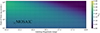 |
Fig. C.1. The maximum value of the ratio between the signal gain per unit observing time for fixed field of view to the same for fixed observing depth, calculated for various telescope fields of view and limiting magnitudes. All values are calculated with reference to a Lyman-α-selected galaxy survey with spectroscopic redshifts used for cross-correlation with a 21-cm measurement from SKA-low, assuming that 21-cm foregrounds extend to the horizon. Values greater than one would indicate that increasing the observing depth yields more signal than increasing the field of view, for the same amount of time spent. All values in the domain shown are less than one, indicating that increasing the field of view yields more signal per unit time than increasing the observing depth. |
All Tables
All Figures
|
Fig. 1. An example 21-cm brightness temperature field at shown at redshifts 6, 7, and 8 (left to right) with galaxies overlaid on zoomed insets (black). Detectable galaxies at these redshifts preferentially reside in ionized regions, with the brightest, most biased galaxies residing in the largest ionized bubbles. The top row shows slices of the full gigaparsec volume used in this study, while the bottom row zooms into a 200 Mpc corner for clarity. Both the brightness temperature and galaxy fields were generated simultaneously using 21cmFASTv4. |
| In the text | |
|
Fig. 2. UV luminosity functions (LFs) at 6≤z≤8 from our fiducial model, compared with several observational estimates. We show Hubble estimates from Bouwens et al. (2021) and Finkelstein et al. (2015), as well as the observation-averaged posterior from Gillet et al. (2020) (1σ credible interval). |
| In the text | |
|
Fig. 3. Lyman-α luminosity functions at z = 6.6. Our fiducial model is based on equivalent width distributions of photometrically selected candidates (see text for details). We also show narrow-band selected LAE LFs from Subaru (Umeda et al. 2025). |
| In the text | |
|
Fig. 4. Schematic illustrating regions in the cylindrical power spectrum that contribute negligibly to the cross-power S/N due to instrument, survey, or systematic limitations. |
| In the text | |
|
Fig. 5. The cylindrical noise power spectra of HERA-350 (top) and SKA-low AA* (bottom) for a fiducial 1000 hour observation at redshift 6.1. The diagonal lines in each panel denote the three choices for wedge excision considered in this work. |
| In the text | |
|
Fig. 6. Power spectra of the galaxy field, 21-cm brightness temperature field, their cross-power spectrum, and the signal-to-noise ratio of the cross-power spectrum as a function of k∥ and k⊥ for a fiducial scenario (left to right). Overlaid are various noise-dominated/excluded regions imposed by systematics and observational effects. The 21-cm brightness temperature power spectrum includes cuts showing the three foreground + instrument (i.e. wedge) contamination scenarios we considered. In this illustrative example, the galaxy survey footprint corresponds to ∼1 sq. deg. at z∼6, and the galaxy redshift uncertainty corresponds to δz∼0.01, which is characteristic of slitless spectroscopy. |
| In the text | |
|
Fig. 7. Distribution of UV continuum magnitudes (MUV) and Lyman-α band AB magnitudes ( |
| In the text | |
|
Fig. 8. Galaxy–21-cm correlation coefficients at z∈(6.2,7.0,8.0,9.0), assuming at two Ly-α magnitude cuts: |
| In the text | |
|
Fig. 9. Effect of observing depth, field of view, and galaxy survey type on the signal-to-noise ratio of a cross-power spectrum detection. Each panel corresponds to a different galaxy survey type, which determines the mean redshift uncertainty associated with that survey. On the top axis of the slit spectroscopy panel, we show the corresponding rest frame UV magnitude limit required for ≥2σ completeness of the photometric candidate sample (see Fig. 7). Blue stars correspond to the SILVERRUSH and MOONRISE high-redshift galaxy surveys, and the orange star corresponds to an overlap of the Roman HLS survey and a single SKA-low AA* beam; multiple 21-cm fields can be tiled to increase the S/N in quadrature as discussed in the text. The MOONRISE spectroscopic survey should enable a 3σ detection of the cross-spectrum. In the spectroscopy panel we also show 100- and 1000-hour isochrones for potential future surveys using MOSAIC on the ELT. |
| In the text | |
|
Fig. 10. As Figure 9, but assuming the pessimistic foregrounds shown in Figure 6. Here, MOONRISE is no longer sufficient for a 3σ cross-spectrum detection, but a 1000-hour survey with MOSAIC remains viable. |
| In the text | |
|
Fig. 11. As Figure 9, but assuming the optimistic foreground scenario in Figure 6. SILVERRUSH remains not viable, although an extremely deep survey of similar angular extent could theoretically breach 3σ, and the S/N with spectroscopy improves only slightly. |
| In the text | |
|
Fig. 12. As Figure 9, but using HERA rather than the SKA-low as the fiducial 21-cm interferometer. Notably, the lack of sensitivity of HERA to high k⊥ modes (i.e. small sky plane scales) precludes detection of the cross-spectrum using a galaxy field with a small (∼5 sq. deg.) field of view. Wide-area slitless spectroscopy remains the only viable candidate for cross-correlating galaxy maps with HERA 21-cm data. |
| In the text | |
|
Fig. 13. Effect of observing depth and field of view on a FRESCO-like survey that selects for Hα at z<7 and [OIII]/Hβ at z≥7. The FRESCO 62 square arcminute fields are too small to yield a detection of the 21-cm cross-power spectrum. |
| In the text | |
|
Fig. 14. Cumulative S/N of the galaxy–21-cm cross-power spectrum as a function of redshift for fiducial observations using MOSAIC, JWST, and Roman. The MOSAIC observation corresponds to our recommended ELT survey, the Roman observation corresponds to and integration over two patches of the SKA-low field of view within the Roman observing area, and the JWST observation corresponds to the FRESCO survey. The Roman and MOSAIC surveys are Ly-α selected, so that redshifts higher than ∼8 contribute negligibly to their total S/N due to attenuation from the neutral IGM. On the other hand, FRESCO selects on Hα and [OIII], allowing higher-redshift galaxies to contribute to the total S/N. The global neutral IGM fraction is indicated on the upper horizontal axis. |
| In the text | |
|
Fig. B.1. The fit function for the signal-to-noise ratio as a function of observing depth for a spectroscopic survey with a field of view of 1 square degree. |
| In the text | |
|
Fig. C.1. The maximum value of the ratio between the signal gain per unit observing time for fixed field of view to the same for fixed observing depth, calculated for various telescope fields of view and limiting magnitudes. All values are calculated with reference to a Lyman-α-selected galaxy survey with spectroscopic redshifts used for cross-correlation with a 21-cm measurement from SKA-low, assuming that 21-cm foregrounds extend to the horizon. Values greater than one would indicate that increasing the observing depth yields more signal than increasing the field of view, for the same amount of time spent. All values in the domain shown are less than one, indicating that increasing the field of view yields more signal per unit time than increasing the observing depth. |
| In the text | |
Current usage metrics show cumulative count of Article Views (full-text article views including HTML views, PDF and ePub downloads, according to the available data) and Abstracts Views on Vision4Press platform.
Data correspond to usage on the plateform after 2015. The current usage metrics is available 48-96 hours after online publication and is updated daily on week days.
Initial download of the metrics may take a while.