| Issue |
A&A
Volume 683, March 2024
|
|
|---|---|---|
| Article Number | A24 | |
| Number of page(s) | 15 | |
| Section | Cosmology (including clusters of galaxies) | |
| DOI | https://doi.org/10.1051/0004-6361/202347591 | |
| Published online | 29 February 2024 | |
The LORELI database: 21 cm signal inference with 3D radiative hydrodynamics simulations
Observatoire de Paris, PSL Research University, Sorbonne Université, CNRS, LERMA, 75014 Paris, France
e-mail: This email address is being protected from spambots. You need JavaScript enabled to view it.
Received:
28
July
2023
Accepted:
23
October
2023
Abstract
The Square Kilometer Array is expected to measure the 21 cm signal from the Epoch of Reionization (EoR) in the coming decade, and its pathfinders may provide a statistical detection even earlier. The currently reported upper limits provide tentative constraints on the astrophysical parameters of the models of the EoR. In order to interpret such data with 3D radiative hydrodynamics simulations using Bayesian inference, we present the latest developments of the LICORICE code. Relying on an implementation of the halo conditional mass function to account for unresolved star formation, this code now allows accurate simulations of the EoR at 2563 resolution. We use this version of LICORICE to produce the first iteration of LORELI, a public dataset now containing hundreds of 21 cm signals computed from radiative hydrodynamics simulations. We train a neural network on LORELI to provide a fast emulator of the LICORICE power spectra, LOREMU, which has ∼5% rms error relative to the simulated signals. LOREMU is used in a Markov chain Monte Carlo framework to perform Bayesian inference, first on a mock observation composed of a simulated signal and thermal noise corresponding to 100 h observations with the SKA. We then apply our inference pipeline to the latest measurements from the HERA interferometer. We report constraints on the X-ray emissivity, and confirm that cold reionization scenarios are unlikely to accurately represent our Universe.
Key words: dark ages / reionization / first stars / radiative transfer / early Universe / methods: numerical
© The Authors 2024
 Open Access article, published by EDP Sciences, under the terms of the Creative Commons Attribution License (https://creativecommons.org/licenses/by/4.0), which permits unrestricted use, distribution, and reproduction in any medium, provided the original work is properly cited.
This article is published in open access under the Subscribe to Open model. This email address is being protected from spambots. You need JavaScript enabled to view it. to support open access publication.
1. Introduction
The first billion years of the evolution of the Universe constitute a key epoch in its development on large scales. Following the hierarchical theory of structure formation and the physics regulating star formation, the gas contained in massive halos cools down, subsequently fragmenting, collapsing, and giving birth to the first stars. This marks the end of the “dark ages” in the history of the Universe. There are several processes responsible for this cooling. The atomic hydrogen cooling channel allows significant cooling down to ∼104 K, that is below the virial temperature of halos with masses of greater than Mmin ≈ 108 M⊙, allowing gravothermal collapse and star formation. Molecular hydrogen cooling brings this minimal mass for star formation down to Mmin ≈ 105 M⊙, in so-called “mini halos”. The emergence of the first stars and galaxies, in a period called Cosmic Dawn (CD, z ∼ 15 − 30), greatly impacted the neutral gas in the intergalactic medium (IGM). Ultraviolet radiation from the first generation of sources ionized their local environment, while the still neutral IGM, farther away from the sources, became heated by X-ray emissions. During the Epoch of Reionization (EoR, z ∼ 6 − 15), the ionized regions quickly grew until they covered the entire IGM. The 21 cm line of neutral hydrogen is emitted by the neutral hydrogen in the IGM and its intensity fluctuations are shaped by the astrophysical properties of the first sources, making it an extremely promising source of information regarding the first billion years of the evolution of the Universe. Furlanetto & Peng (2006) provide a review of this topic.
While valuable, the detection of this signal remains an observational challenge. Foreground emissions, which are roughly 10 000 times stronger than the expected intensity of the 21 cm signal, must be subtracted from observed data or avoided in order to extract the cosmological signal. The subtraction requires the very good handling of radio frequency interference, a deep and exact sky model, and accurate direction-dependent calibration (see e.g. Mertens et al. 2020). Many instrumental programs are tackling this challenge, the most ambitious being the Square Kilometer Array (SKA). The unprecedented sensitivity of the SKA will enable us to probe this epoch with sufficient signal-to-noise ratio to build a full tomography of the signal between z ∼ 27 and z ∼ 6, providing a comprehensive view of how reionization unfolded. The observation of the 21 cm signal by the SKA will start by the end of this decade, but several instruments are already trying to measure summary statistics of the signal. A first detection of the global (sky-averaged) signal at z ∼ 16 was announced by Bowman et al. (2018), who used the Experiment to Detect the Global EoR Signature (EDGES) instrument. The features of this detection, in particular the strong intensity of the signal in absorption, are not compatible with standard models of reionization and this result has not been confirmed by other global signal experiments, such as SARAS-3 (Singh & Nambissan 2022). Interferometers such as the Low-Frequency Array (LOFAR), the Murchison Widefield Array (MWA), the New Extension in Nançay Upgrading LOFAR (NenuFAR), and the Hydrogen Epoch of Reionization Array (HERA) aim to measure the power spectrum of the 21 cm signal. While no detection has yet been claimed, upper limits on the spectrum have been devised (e.g., Mertens et al. 2020; Trott et al. 2020; Abdurashidova et al. 2023; Munshi et al., in prep., and references therein). In the coming years, these instruments are expected to detect the signal or to produce upper limits that are informative enough to constrain nonexotic models of the EoR at various scales and redshifts. Given these observational prospects, in order to extract astrophysical information, the community must provide accurate models of the first billion years of evolution of the Universe, as well as inference methods linking raw observational data to the astrophysical processes encoded in the models.
On the one hand, sustained effort has been put into developing theoretical and numerical approaches to model the EoR, ranging from fast semi-analytical codes (e.g., Mesinger et al. 2011; Santos et al. 2010; Cohen et al. 2017; Murray et al. 2020; Reis et al. 2021) to expensive 3D radiative transfer simulations (e.g., Ciardi et al. 2003; Mellema et al. 2006; Baek et al. 2010; Semelin et al. 2017; Ocvirk et al. 2020; Lewis et al. 2022; Doussot & Semelin 2022). Fast codes compute the dynamics of dark matter in the linear regime and typically assume a constant gas-to-dark-matter density ratio. On large scales (more than a few cMpc), this yields similar results to full numerical simulations that compute the nonlinear dynamics of gravity and hydrodynamics. However, star formation, a crucial process when modeling the EoR, occurs on small scales. This leads to very different modeling approaches. In high-resolution N-body simulations, individual dark matter halos are resolved. Star formation within the halos can then be computed from the local properties of the gas (typically density and temperature), though the actual equations linking gas properties to star formation may differ between simulation codes. One-dimensional (spherically symmetric) radiative transfer simulations assign baryons to halos formed in pre-computed dark-matter-only simulations (Krause et al. 2018; Ghara et al. 2018; Schaeffer et al. 2023) using simple recipes, and compute star formation from there. Semi-analytical codes usually do not resolve individual halos but estimate populations of halos and stars in a given region, through for instance the CMF formalism (Lacey & Cole 1993). These different modeling approaches can potentially induce different features in the reionization field. The second critical step is the process through which UV and X-rays are accounted for. Fully numerical simulations typically include 3D radiative transfer through the use of M1 or various ray-tracing methods, while semi-analytical codes identify ionized and heated regions through simple (and easy to compute) photon budget arguments. A comprehensive evaluation of the impact of these different modeling approaches on the interpretation of the 21 cm signal remains to be performed.
On the other hand, applications of inference methods to the 21 cm signal have been under development in the last 10 yr. The most widely employed technique is undoubtedly the Markov chain Monte Carlo (MCMC) algorithm (see e.g., Greig & Mesinger 2015, 2018; Schmit & Pritchard 2018). In this approach, the posterior distribution of the parameters is explored in a guided random walk. This method is guaranteed to converge towards the true posterior probability (under some reasonable assumptions). However, it requires that an explicit likelihood can be formulated and it might require hundreds of thousands or millions of steps (and thus of realisations of the model) to produce a good estimate of the posterior, making its use only suited to fast numerical codes. This led the community to explore other inference techniques, such as training artificial neural networks to do the inference (Shimabukuro & Semelin 2017; Doussot et al. 2019; Kendall & Gal 2017; Neutsch et al. 2022). While requiring fewer simulations in the training sample, convergence towards the true maximum likelihood or true posterior is in this case not guaranteed, as the training of the neural network can produce a systematic bias or a residual additional variance. Another noteworthy family of methods is called “simulation-based inference” or “likelihood-free inference” (Alsing et al. 2018; Alsing & Wandelt 2018; Zhao et al. 2022; Prelogović & Mesinger 2023). These methods rely on the fact that a simulation is in and of itself a draw in the joint probability of the observable data and the model parameter, a joint probability that need not necessarily be explicitly writable. The joint probability distribution is then fitted using a neural network acting as a parametric function, allowing the straightforward computation of the posterior.
Due to computation time constraints, most inference methods have until now only been applied to signals generated using semi-numerical approaches, as they typically are a hundred thousand times faster than fully numerical simulations. Indeed, performing a single MCMC inference with the LICORICE code, for example, running at high resolution would require 1011 CPU hours of computation, well beyond current capabilities. Performing inference with such a code at a reasonable cost therefore requires the use of machine-learning-based approaches, which can reduce the number of simulations to a few thousand. However, even in this case, a decrease in resolution is necessary to reach an affordable computing cost. This decrease must be compensated for by a significant amount of subgrid modeling. This constitutes the approach at the heart of this work, where we use of the order of 103 simulations to chart a 4D astrophysical parameters space with 2563 simulations in 300 cMpc boxes. When then train neural network emulators for the power spectrum of the signal and use them to perform MCMC inference.
In this paper, we present LORELI, a collection of numerical simulations of the EoR using the LICORICE code. In Sect. 2, we explain the recent modifications of the code that make such a database possible. In Sect. 3, we give details about the LORELI database, and in Sect. 4, we show the results of parameter inference applied to both mock data and the most recent data from the HERA Collaboration (Abdurashidova et al. 2022), which we obtain using an emulator of the code trained on LORELI.
2. The LICORICE code
The simulations of the LORELI dataset were run using the LICORICE simulation code (Semelin et al. 2007, 2017; Baek et al. 2009; Semelin 2016). Here, we provide a brief overview of the code and details about recent developments. LICORICE is an N-body simulation code dealing with baryons and dark matter particles. Dynamics is solved using a TREE+SPH method (Springel et al. 2001). Radiative transfer in UV and X-ray continuum is coupled to dynamics through a Monte-Carlo scheme on an adaptive grid: photon packets are emitted in random directions by source particles (baryon particles with a nonzero stellar fraction), propagate at the speed of light, redshift, and deposit their energy in gas particles lying in the encountered cells depending on local density. They represent UV ionizing radiation and X-rays. “Hard” X-rays, after propagating over a distance larger than the size of the simulation box, are added to a uniform background. The ionization and temperature states of each gas particle are then updated several times per dynamical time step and the latter affect dynamics through the pressure and artificial viscosity terms in the SPH scheme (Monaghan 1992; Springel et al. 2001).
2.1. Star formation model
In previous iterations of LICORICE, gas particles with an SPH-calculated overdensity δ greater than a fixed threshold δthresh transform – at each dynamical time step – a fraction of their gas mass into stellar mass following a Schmidt-Kennicutt law of exponent one, using
 (1)
(1)
where f* is the current stellar fraction of the particle, fcoll = 1 if δ > δthresh and f* otherwise, df* is the newly created stellar fraction, dt the duration of a time step, and τ is an astrophysical parameter of the simulation representing the typical gas-to-stars conversion timescale, thus controlling the star formation rate (SFR). However, this star formation numerical method is sensitive to an insufficient resolution: failure to resolve the small-scale modes of the density field will smooth out the density peaks and prevent particles from reaching the density threshold for star formation, causing Eq. (1) to underestimate the SFR. Essentially, a simulation will lack the star formation of unresolved star-forming halos. The mass of the lightest of these halos is estimated to be ∼108 M⊙, as it corresponds to a virial temperature of 104 K, the lowest temperature reached through the cooling of atomic hydrogen. In boxes of hundreds of cMpc, which is large enough to capture relevant large-scale fluctuations of the 21 cm signal, resolving such halos requires more than 40963 particles and 107 ∼ 8 cpuh. This motivates a new implementation in the code of a subgrid model designed to provide a better estimate of star formation in unresolved halos, without affecting resolved ones.
2.2. The conditional mass function subgrid model
The chosen subgrid model relies on the conditional mass function (CMF) formalism (Lacey & Cole 1993) to estimate the halo mass functions of regions below the spatial resolution limit. In the CMF theory, the density of spheres of decreasing radii follows a random walk, and statistically estimating the radius at which the threshold δc is crossed for the first time gives the CMF of regions parameterized by their radius R0 and overdensity δ0.
In extended Press-Schechter (EPS), the simplest formulation of the CMF theory, the fraction of the mass of a region (again parameterized by a radius R0 and overdensity δ0) that lies in collapsed halos more massive than Mmin is given by
![Mathematical equation: $$ \begin{aligned} f_{\rm coll} = \mathrm{erfc}\left[ \frac{\delta _{\rm c}-\delta _0}{\sqrt{2(\sigma (M_{\rm min})^2 - \sigma _0^2 })}\right] ,\end{aligned} $$](/articles/aa/full_html/2024/03/aa47591-23/aa47591-23-eq2.gif) (2)
(2)
where σ(M) is the density variance on mass scale M and δc is the linear overdensity of collapse. The classical theory of structure formation predicts δc ≈ 1.68.
Sheth et al. (2001) devised a more accurate formalism (ST) to calculate the mass function. During the random walk, instead of crossing a constant threshold of size δc, a “moving barrier”
![Mathematical equation: $$ \begin{aligned} B(\sigma ^2, z) = \sqrt{a}\delta _{\rm c}[1 + \beta (a\frac{\delta _{\rm c}^2}{\sigma ^2})^{-\alpha }] \end{aligned} $$](/articles/aa/full_html/2024/03/aa47591-23/aa47591-23-eq3.gif) (3)
(3)
is adopted. This extends the EPS formalism from the physics of spherical collapse to that of ellipsoidal collapse. α ≈ 0.615, β ≈ 0.485 are parameters whose values come from ellipsoidal dynamics and a ≈ 0.707 is fitted to accurately model simulations. Rubiño-Martín et al. (2008), Tramonte et al. (2017) provided an expression for the CMF associated with ST:
![Mathematical equation: $$ \begin{aligned} n_{\rm c}(M) = -\sqrt{\frac{2}{\pi }}\frac{\mathrm{d}\sigma }{\mathrm{d}M} \frac{\rho _0}{M} \frac{|T(\sigma ^2 | \sigma _0^2)|\sigma }{(\sigma ^2- \sigma _0^2)^{3/2}} \mathrm{exp} \left[ -\frac{(B(\sigma ^2, z) - \delta _0)^2}{2(\sigma ^2 - \sigma _0^2)} \right] , \end{aligned} $$](/articles/aa/full_html/2024/03/aa47591-23/aa47591-23-eq4.gif) (4)
(4)
where
![Mathematical equation: $$ \begin{aligned} T(\sigma ^2 | \sigma _0^2) = \sum ^5_{n=0} \frac{(\sigma _0^2 - \sigma ^2)^n}{n!} \frac{\partial ^n[B(\sigma ^2, z) - \delta _0]}{\partial (\sigma ^2)^n}. \end{aligned} $$](/articles/aa/full_html/2024/03/aa47591-23/aa47591-23-eq5.gif) (5)
(5)
One can then easily calculate Mcoll, the mass of the region contained in halos more massive than Mmin:
 (6)
(6)
where Vregion is the Lagrangian volume of the region and Mregion its mass. We then calculate the collapsed fraction as
 (7)
(7)
Both EPS and ST CMFs are implemented in the version of LICORICE used in the present work. In practice, we calculate fcoll for each gas particle. To do so, we calculate the overdensity  of the region they represent, where ρ0 is the SPH-calculated density of the particle multiplied by the cosmological ratio Ωm/Ωb. The volume of the region is given by
  , where R0 is the SPH smoothing radius. While the formulation of the CMFs relies on top-hat filters, the SPH smoothing kernel is not a top-hat, and so the γ parameter is tuned to represent the volume of the region of identical density smoothed with a top-hat kernel. Motivated by the fact that the integral of the SPH kernel reaches 99% of its maximum value past ∼0.7R0, we find γ = 0.4 to be a reasonable choice, and indeed this choice is validated by the resolution study presented below.
We use the resulting value of fcoll in Eq. (1) instead of setting fcoll depending on some density threshold. This is done either with Eq. (2) when using the EPS formalism, or with Eqs. (4), (6) and (7) when using ST.
A final subtlety lies in the fact that in LICORICE, all gas particles with a nonzero stellar fraction are considered sources of photons. However, this CMF formalism assigns a strictly positive fcoll to all particles. This causes particles to behave in an unphysical manner, as they instantly turn into sources at the beginning of the simulation with infinitesimal stellar fractions. To avoid this, a method to stochastically assign fcoll was adopted: when dfcoll, the difference in fcoll of a particle between one time step and the next, is smaller than  , dfcoll, min is assigned to the particle with a probability
  . This effectively prevents very weak, unphysical star formation at very high redshifts (z ≳ 25 − 30 depending on Mmin, approximately when star formation starts in high-resolution simulations) while ensuring that the average star formation density (SFRD) remains identical to that of the nonstochastic model.
Figure 1 shows how the HMF of HIRRAH-21, a high-resolution LICORICE simulation (20483 particles, with no subgrid model) presented in Doussot & Semelin (2022), compares with the PS and ST models at different redshifts. The HMF of HIRRAH-21 was calculated by finding halos in the simulation using a Friends-of-Friends (FoF) algorithm. We find excellent agreement with the ST HMF, which lies a couple orders of magnitude above the PS HMF. This is not unexpected, given the findings of Reed et al. (2007), and this difference in the HMFs necessarily appears in the CMFs. This justifies the implementation and use of the ST CMF. However, for practical reasons, in the presented and current version of the LoReLi database, we compute star formation using EPS and a different choice of an effective radius (10% smaller, which implies a ∼5% larger σ) that produces a very similar SFRD. Future versions of the database will use the ST CMF. A comparison of the conditional mass functions of HIRRAH-21 at z = 9.48 with the prediction of ST and EPS (with a σ scaled up by 5%) at different overdensities δ can be seen in Fig. 2. Good agreement between simulation and models is observed, with errors roughly within the fluctuations in the simulated CMF due to cosmic variance. The resulting fcoll are within ∼30% of each other.
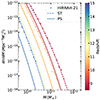 |
Fig. 1. Evolution with redshift of the halo mass function of HIRRAH-21, calculated using a FoF algorithm. We also show the history of theoretical PS and ST HMFs for the same cosmology. |
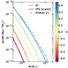 |
Fig. 2. Evolution of the simulated CMF with the overdensity δ and of the theoretical CMFs as predicted by the ST and EPS models. In order to match the high-resolution simulation, the σ in the EPS model has been scaled up by 5% on average. |
However, the connection between the simulated HMFs and star formation in the simulation is indirect, as star formation in LICORICE does not necessarily occur in identified dark matter halos: only the local density of the gas appears in the star formation equation and not the properties of the dark matter that may or may not be present nearby. In order to evaluate the results of this subgrid model on star formation, we compare in Fig. 3 the star formation rate density (SFRD) of HIRRAH-21 and LORRAH-21, a low-resolution simulation (2563 particles with the subgrid modeling of star formation). The Mmin parameter of the subgrid model was set at 4 × 10⁹ M⊙ to match the mass of the lightest halos identified by FoF in HIRRAH-21, and all other astrophysical and numerical parameters are identical in the two setups except for the dynamical time step: 0.5 Myr in HIRRAH-21 and 7 Myr in LORRAH-21. We observe very good agreement between the SFRDs of LORRAH-21 and HIRRAH-21 over the entire redshift range (with an RMS of the relative error of 0.16 between z ∼ 20 and z ∼ 7, and of 0.09 between z ∼ 15 and z ∼ 7). The largest mismatch (∼30%) occurs at z ∼ 18 − 20, when the stochastic attribution of fcoll is the most relevant. In order to test this subgrid model at a different resolution, Fig. 3 also shows the SFRD in a 10243 simulation (from the 21SSD database Semelin et al. 2017) with the same parameters as HIRRAH-21 (but a minimal mass of DM halos naturally set to 3.2 × 10¹⁰ M⊙) and in LORRAH-21, this time with Mmin set to the same value. In this case as well, excellent agreement is observed, implying that this CMF formalism is robust to resolution and can accurately describe the behavior of simulations of higher resolution.
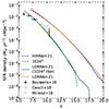 |
Fig. 3. History of the SFR of HIRRAH-21 and LORRAH-21. As a reference, observational data from Bouwens et al. (2016), Oesch et al. (2018), McLeod et al. (2016) are included. The SFRD of a 10243 particles simulation is also plotted, and is consistent with that of a LORRAH-21 simulation using a Mmin parameter set at the value of the smallest resolved halos in the 10243 simulation. |
2.3. Two-phase model of gas particles
The other significant adaptation of the code is the computation of a specific temperature for the neutral phase within each gas particle. In previous versions of the code, only the average temperature of particles was considered (see Baek et al. 2009 for details) and used in 21 cm computations. This may have no consequence in high-resolution simulations, as ionization fronts are resolved, but becomes an issue as the resolution decreases. Low resolution implies a high number of partially ionized particles that actually represent a fully neutral phase and a fully ionized phase, and using the phase-averaged temperature then leads to a poor estimation of the intensity of the 21 cm signal. Indeed, the average temperature between the neutral and ionized gas is greater than the temperature of the neutral phase alone, often by orders of magnitude. This does not affect codes that do not allow partial ionization, such as 21CMFAST (Mesinger & Furlanetto 2007), and post-processing solutions have been designed to correct for this effect with the significant drawback of having to run additional simulations without X-rays (Ross et al. 2017). To compute the temperature of the neutral phase in LICORICE, only the coupling to the dynamics, the cosmological adiabatic expansion of the gas, and the heating by X-rays were considered. This means computing the temperature evolution equation in Baek et al. (2009) with only the HI atoms:
![Mathematical equation: $$ \begin{aligned} \frac{\mathrm{d}T_{\rm HI}}{\mathrm{d}t} = \frac{2}{3 k_{\rm B} n_{\rm HI}}\left[ - \frac{3}{2}k_{\rm B} T_{\rm HI}\frac{\mathrm{d}n_{\rm HI}}{\mathrm{d}t} + \Lambda \right] ,\end{aligned} $$](/articles/aa/full_html/2024/03/aa47591-23/aa47591-23-eq12.gif) (8)
(8)
where Λ contains the X-ray heating and the adiabatic temperature evolution of the gas due to the dynamics, as well as the viscosity term of the SPH algorithm from Monaghan (1992), all computed independently for the neutral phase. This equation describes the evolution of the internal energy of the neutral phase of a particle when interacting with the other particles in the SPH scheme.
The resulting evolution of temperatures is shown in Fig. 4. These results confirm that, after the start of reionization (z ≲ 13), the temperature of the neutral phase of particles in LORRAH-21 is more than an order of magnitude below their average temperature and on average significantly lower than the temperature of weakly ionized (≲2%) particles. This temperature is much closer to the temperature of weakly ionized particles of HIRRAH-21, which is used as an imperfect proxy for the temperature of the neutral phase in HIRRAH-21, which was not implemented at the time.
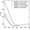 |
Fig. 4. History of the average temperature of all particles in both LORRAH-21 and HIRRAH-21, as well as the temperature of weakly (< 2%) ionized particles. In the case of LORRAH-21, the temperature of the neutral phase of the particles is also shown. |
A decrease in resolution also affects the recombination rate R of the ionized gas, as it depends on the square of the HII density. The main theoretical approach to counter this effect is to use a clumping factor. Different versions of the clumping factor (inspired by different works : Kaurov & Gnedin 2014; Mao et al. 2020; Chen et al. 2020; Bianco et al. 2021) have been implemented in LICORICE. However, none of them managed to reconcile the reionization timings of LORRAH-21 and HIRRAH-21.
The main cause of this failure is that any error in the calibration of the parameters of the implemented clumping factor formula will cause an error in the average ionized fraction in the simulated box that increases with time. For instance, too small a clumping factor at a time step n will cause too few HII to recombine, leaving too many photons per HI at time step n + 1, further increasing the HII density. In conclusion, none of the theoretical approaches to the clumping factor or fit to high-resolution simulations available in the literature were accurate enough, and matching the reionization timings of our low- and high-resolution simulations required a calibration of the photon budget instead. To do so, a “step” model of the UV escape fraction fesc was implemented in LORRAH-21, depending on the local ionization fraction xion:
 (9)
(9)
where fesc, post = 0.1, fesc, pre = 0.01, and xthresh = 0.01 are parameters of this model, calibrated on HIRRAH-21 for LORRAH-21. This is justified by the fact that the recombinations missing in LORRAH-21 occur in unresolved dense regions that are likely to surround the unresolved sources and must be ionized before letting the UV photons escape the ∼1 Mpc region represented by a gas particle. The ionization history of LORRAH-21 using this model is consistent with that of HIRRAH-21, which is something that was not observed when the simulation code relied on a clumping factor implementation. However, an approach using the clumping factor that leads to equivalent or more accurate results might be found in the future.
The global 21 cm signals of HIRRAH-21 and LORRAH-21 (calculated with the average temperature and with the HI temperature) are shown in Fig. 5. As expected, the 21 cm signal is strongly modified when calculated with the phase-averaged temperature when compared to the result obtained using the HI temperature. In addition, the 21 cm signal of LORRAH-21 calculated using the HI temperature is in good agreement with the signal in HIRRAH-21. A small mismatch occurs at z ≲ 11, as heating occurs in LORRAH-21 approximately 0.15 redshift units before HIRRAH-21, which is mainly due to the slight difference in SFRD. Over the whole redshift range, LORRAH-21 is a good approximation of HIRRAH-21, especially given the 104 increase in computation speed in LORRAH-21 caused by the drop in resolution: HIRRAH-21 required ∼3 × 10⁶ cpuh (which is why it was not run again with the newly implemented subgrid models) while running LORRAH-21 only takes ∼3 × 10² cpuh.
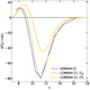 |
Fig. 5. Global 21 cm signal in HIRRAH-21 and LORRAH-21, the latter calculated using either the phase-averaged temperature ⟨T⟩ of particles or the temperature of their neutral phase THI. This shows that properly taking into account the temperature of the neutral phase is critical in order to correctly model the 21 cm signal in low-resolution numerical simulations. |
3. The LORELI database
We now present the LORELI database1, which consists of 760 simulations with 2563 resolution elements run in 300 Mpc boxes using the code presented in the previous section, including the subgrid models for unresolved sources and the computation of the neutral phase temperature for each particle. Initial conditions, generated using the MUSIC code (Hahn & Abel 2011), vary between simulations. The four-parameter space sampled by the database was designed to loosely constrain parameter values according to various probes of reionization. Here are the varied parameters and explored ranges:
-
The gas-to-star conversion timescale τ ∈ [10 Gyr, 100 Gyr] and minimum halo mass Mmin ∈ [108 M⊙, 4 × 10⁹ M⊙] are the parameters of the star formation model.
-
fesc, post ∈ {0:05; 0:1; 0:2; 0:3; 0:4; 0:5} is the escape fraction of UV radiation in particles with an ionized fraction of higher than xthresh.
-
The X-ray production efficiency fx ∈ [0.1, 10], in nine logarithmically spaced values. This drives the X-ray emissivity according to
 (Furlanetto & Peng 2006).
Only astrophysical parameters were varied: cosmology was kept constant across the database. Due to computation time constraints, fesc, pre and xthresh were not varied and were kept at 0.01, the same as in LORRAH-21. We expect these parameters to have a smaller impact on the global ionization field (except at high redshift) as the local ionization rises above the threshold early in the source life. Numerical and cosmological parameters are detailed in Table 1.
Numerical and cosmological parameters of LORELI simulations.
3.1. Observational constraints
Here we describe the regions of the parameter space that were explored and the observational constraints we used to restrict these regions. We also present the evolution of different relevant physical quantities in the LORELI simulations.
3.1.1. Star formation rate
The star formation parameters τ and Mmin were constrained using recent observations of high-redshift galaxies and SFR estimates by Bouwens et al. (2016), McLeod et al. (2016), and Oesch et al. (2018). A χ2 test was performed to exclude models that fit none of the considered observational data sets with a probability of higher than 5 %. Seventeen {τ, Mmin} couples were selected and the range of SFRD spanned in our database can be seen in Fig. 6. Measurements acquired with the JWST are likely to give tighter and higher redshift constraints in the near future.
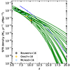 |
Fig. 6. Star formation rate density history for the 17 (τ, Mmin) parameter couples used in LORELI simulations (solid). The parameters were selected from a grid after a χ2 goodness-of-fit test. Only the parameter couples yielding a p-value p such that 1 − p < 0.95 for at least one of the plotted observational data sets were kept from the initial grid. For reference, the SFR in HIRRAH-21 is also plotted (dashed). |
3.1.2. The Thomson scattering optical depth
As late reionization scenarios are disfavored by several reionization probes (Fan et al. 2006; Mitra et al. 2011; Greig et al. 2019), fesc values were chosen so that reionization in LORELI ends between z ∼ 5 and z ∼ 8. Reionization history can also be characterized based on the Thomson optical depth τT. The values of τT of the LORELI simulations are shown in Fig. 7 along with the results from the Planck Collaboration (Planck Collaboration XIII 2016; Planck Collaboration VI 2020). While we did not use this observation to constrain the parameter space of LORELI, nearly all models are within 3σ of the mean value in Planck 2018 cosmology and within 1σ of that of Planck 2015. We note that the value obtained in Planck 2018 assumes simple models for reionization, and we do not exclude the couple LORELI simulations that display a ≳3σ tension from the dataset.
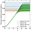 |
Fig. 7. Thomson optical depth of the LORELI signals. The ionization histories of the simulations confine the optical depths to within 1σ of Planck’s 2015 measurement (dotted: central value, shaded region: 1σ). As in 21SSD (Semelin et al. 2017), the second ionization of He is assumed to occur at z = 3. |
No other constraints on reionization history were applied. In particular, no attempt was made to match observational data on the evolution of the global average ionized fraction ⟨xHII⟩, as calibrating the escape fraction parameters for each {τ, Mmin} couple would require many simulations. For completeness, we plot the evolution of ⟨xHII⟩ for all LORELI simulations in Fig. 8.
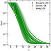 |
Fig. 8. Average ionization fraction of the LORELI models, as well as observations from Bouwens et al. (2015), Davies et al. (2018), Wang et al. (2020). These observations were not used to calibrate the database, and reionization ends in all models between z ∼ 8 and z ∼ 5. |
3.2. 21 cm signals in LORELI
The differential brightness δTb of each 21 cm signal in LORELI was computed according to, for example, Furlanetto & Peng (2006):
![Mathematical equation: $$ \begin{aligned} \begin{aligned} \delta T_b&= 27 x_{HI}(1+\delta ) \left[ \frac{T_s - T_{\rm CMB}}{T_s} \right] \left[ 1 + \frac{\mathrm{d}{ v}_{||}/\mathrm{d}r_{||}}{ H(z) } \right]^{-1} \\&\times \left[ \frac{1+z}{10}\right]^{1/2} \left[ \frac{\Omega _b}{0.044} \frac{h}{0.7} \right] \left[ \frac{\Omega _m}{0.27}\right]^{1/2} \, \mathrm{mK,} \end{aligned} \end{aligned} $$](/articles/aa/full_html/2024/03/aa47591-23/aa47591-23-eq15.gif) (10)
(10)
where xHI is the local neutral fraction, δ the local overdensity, Ts the spin temperature of neutral hydrogen, TCMB the CMB temperature at redshift z, H(z) the Hubble parameter, and dv||/dr|| the velocity gradient along the line of sight. The spin temperature was calculated from simulated data according to the classical equation (see e.g., Furlanetto & Peng 2006) :
 (11)
(11)
where Tkin is the kinetic temperature of hydrogen, and xc and xα the collisional and Wouthuysen-Field couplings, respectively. Collisional coupling is negligible in the considered redshift range, and therefore coupling to Tkin is driven by the Wouthuysen-Field effect (Wouthuysen 1952). xα was computed on all saved snapshots for all simulations in a post-processing step using the semi-analytical code SPINTER (Semelin et al. 2023). The luminosities of LICORICE particles were arranged on a 2563 grid, which SPINTER takes as input. SPINTER computes spherically symmetric propagation kernels using MCMC ray tracing that accounts for scattering in the wings of Lyman-α line. These kernels are then convolved with the emissivity field at previous redshifts to output grids of xα. The outputs of SPINTER are close to those of full radiative transfer in the Lyman bands, and calculating xα for a single simulation takes a few CPU hours, making the cost of this post-processing step negligible. We show every global 21 cm signal in Fig. 9. In its current state, the database contains a wide range of models that can be considered fiducial: these are shaped by conservative observational constraints and no “exotic” physics are included, such as nonstandard dark matter (Barkana 2018) or extra radio background (Fialkov & Barkana 2019). In particular, the EDGES measurements are not compatible with any of the LORELI signals, as the absorption peaks of LORELI signals are shallower at lower redshifts, and have milder slopes than EDGES-compatible signals. However, some of these exotic physics, such as the extra radio background, can easily be computed in post-processing steps from LORELI snapshots.
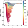 |
Fig. 9. Global 21 cm brightness temperature of the LORELI simulations. As opposed to 21SSD, global brightness temperatures are calculated from full 3D snapshots, not single slices of lightcones, and therefore do not exhibit small redshift-scale fluctuations. Color represents the value of fX, the parameter which impacts the depth of the signal the most. |
4. Inference on power spectra
In the previous section, we detail the set of simulations at our disposal. However, simulating many scenarios of the EoR is only the first step toward understanding how reionization took place in our Universe. Indeed, one must then be able to extract information from observations to determine which model is the likeliest. In this section, we present how we perform this inference step using the LORELI dataset, first on mock data and then on actual observations from the HERA instrument. LORELI contains raw snapshots and lightcones containing full particle information at 55 redshifts between 53.6 and 4.97, as well as various physical quantities on 3D grids (data cubes). However, in order to compare models to future observational data, it is convenient to compress this high-dimensional data into summary statistics. The most common choice is the 3D power spectrum of the 21 cm signal, which various instruments are currently trying to measure (Patil et al. 2017; Mertens et al. 2020; Trott et al. 2020; Abdurashidova et al. 2023). While it does not contain non-Gaussian information, and summaries representing complementary information do exist, we focus on the power spectrum in the following. We show the power spectra of the LORELI simulations in Figs. 10 and 11, as well as upper limits from recent observations, and expected thermal noises of various instruments. The power spectra were calculated using the coeval cubes of the signal and not the lightcones. This approximation can have a significant (up to ∼50%) effect on the spectrum (Datta et al. 2012, 2014) and taking this into account will be at the center of future improvements of our method. As expected from classical 21 cm theory, at higher redshift, the amplitude of the spectra is mostly driven by the Lyman-α coupling, and becomes primarily dictated by the value of fX at lower redshifts. We anticipate that improvements of these upper limits in the coming years will soon allow tight constraints on our models.
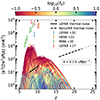 |
Fig. 10. Power spectra of the LORELI simulations at k = 0.1 h/cMpc as a function of z. These are compared to recent upper limits of various instruments (Patil et al. 2017; Mertens et al. 2020; Trott et al. 2020; Abdurashidova et al. 2023) as well as theoretical thermal noise power of 1000 h observations with NenuFAR and LOFAR. |
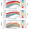 |
Fig. 11. Power spectra of LORELI models as a function of k at redshifts of 9, 11, and 14, from top to bottom. The value of the SKA thermal noise (1000 h of observation) is plotted to demonstrate that the LORELI signals should be detectable by the instrument. |
Classical Bayesian inference, for example through the use of MCMC, requires large numbers of forward modeling instances (≳105), often sequentially. Given the computation cost of a single LICORICE simulation, this is unreasonable even at 2563 resolution. In order to perform parameter inference on this power spectra dataset, our method consists in using LORELI as a training sample for a neural network that will function as an emulator of LICORICE, and then performing classical MCMC inference using the emulator as the model. Indeed, once the emulator is trained, the computation cost of producing a single signal drops to a few milliseconds, which allows a sufficiently large number of steps to be completed in the Markov chain in a few hours of runtime.
4.1. Data preprocessing
4.1.1. Data properties
In order to efficiently train the network, it is necessary to preprocess the data. The power spectra were computed for a list of 32 redshifts, with power spectra being set to zero for z between the redshift of full reionization and the last redshift bin. However, in order to reduce the dimensionality of the problem, we restrict our analysis to k = [0.23, 0.33, 0.46, 0.66, 0.93, 1.31, 1.86, 2.64h cMpc−1] and z = [15.67, 14.05, 12.77, 11.73, 10.87, 10.14, 9.51, 8.96]. The k bins width is defined such that the bins do not overlap. The 21 cm power spectra span many orders of magnitude, which tends to hinder the training of networks. Therefore, the logarithm of the power spectra was used before normalizing by dividing by the maximum value across the dataset.
4.1.2. Noise in the signals
For an inference framework to have any practical application, it must be performed on signals affected by instrumental effects. Here we neglect foreground residuals and other systematics and focus on the SKA thermal noise for an observation time of 100 h. As in Doussot et al. (2019), and following McQuinn et al. (2006), the standard deviation of the power spectrum caused by SKA thermal noise was computed as
![Mathematical equation: $$ \begin{aligned} \delta P(k,z) = \left[\sum _{|k| = k}\left( \frac{1}{ \frac{Ax^2 y }{\lambda (z)^2 B^2} C(\mathbf k ,\mathbf k ) } \right)^2 \right]^{-1/2} ,\end{aligned} $$](/articles/aa/full_html/2024/03/aa47591-23/aa47591-23-eq17.gif) (12)
(12)
where λ is the observed wavelength, A the area of a 256-antenna station, B = 10 MHz is the bandwidth, x the comoving distance to the observed redshift, y the depth of field, and C the detector covariance matrix. In order to noise a signal, we simply add a realization of a Gaussian random variable of mean 0 and standard deviation δP(k, z) for each k, z.
This noise is added to another form of stochasticity, the cosmic variance of the simulation box (CV), which is implicit to our setup. We recall the equation found in McQuinn et al. (2006) to compute the covariance matrix of CV, which is added to the detector noise covariance matrix in the previous equation:
 (13)
(13)
Marginalizing over CV for each point in parameter space requires hundreds of simulations at each point and is not feasible using LORELI. However, as CV mainly affects the largest scales, its effect can be at least partially avoided by focusing the analysis on k ≳ 0.1 h cMpc−1. This motivates us to focus our analysis on a region in k-space more affected by thermal noise, which is far less computationally expensive to generate. It is also likely that a machine learning method that tends to interpolate between the LORELI simulations, such as the one presented in the following section, smooths over the effects of CV altogether.
4.2. LOREMU
LOREMU, an emulator of the LICORICE power spectra, was trained using the LORELI simulations. The network is a multilayer perceptron that takes the four astrophysical parameters and a (k, z) pair as inputs, and outputs a noiseless power spectrum value. The full architecture and parameters are shown in Table 22 and were implemented using the Keras framework (Chollet 2015). LOREMU was trained in a supervised manner to predict the value of the (noiseless) power spectrum given the inputs k, z, and the astrophysical parameter values. Training took place over 200 epochs, using a batch size of 32, and minimizing a mean squared error (MSE) loss function using the Adam optimizer with a learning rate of 5 × 10⁻⁴. The training set was composed of a randomly selected 75% of the 760 spectra, while the remaining 25% of the spectra were set aside to constitute the test set.
Architecture and hyperparameters of LOREMU.
This network is deterministic. In particular, this means the output power spectra do not include a proper contribution by CV. It is hypothesized that the emulator learns to average over the CV affecting the large scales, as the spectra in the training set that are close in parameter space have been generated using different initial conditions of the density field and therefore have different CV realizations. Various quantities describing the accuracy of the emulator are depicted in Fig. 12. As indicated by the bottom left plot, the emulator performs especially well at high k and low redshifts. At large scales, the error is caused by the fact that the emulator cannot predict CV, whereas spectra in the test set include a CV realization (see top right plot). At high redshift, the signal is faint, resulting in low loss but high relative error (see bottom plots). The rise in relative error at the very lowest redshift may partially be due to simulations approaching the end of reionization, but is in this case accompanied by a rise in the loss function, which is more difficult to explain. A similar issue was found to occur by Jennings et al. (2019), and this region in (k, z) may be the focus of future improvements of the emulator. Overall, our emulator outperforms that of Jennings et al. (2019) by a factor of ∼2. We show examples of simulated and emulated signals in Fig. 13.
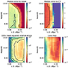 |
Fig. 12. Diagnostics of the performance of the emulator. Top left: At each k, z, median across the dataset of the emulator error-to-thermal-noise ratio. Top right: At each k, z, median across the dataset of the emulator error-to-cosmic-variance ratio. The error increases with cosmic variance, as the deterministic network cannot replicate the noise induced by cosmic variance. Bottom left: 100x mean squared relative error across the dataset between the emulator prediction and the training sample. Bottom right: Loss at each k, z. Faint signal at high z causes low loss but high relative error. Cosmic variance causes high loss and relative error at low k. Additionally, we checked that the mean square relative error exhibits no systematic trend depending on the values of the astrophysical parameters. |
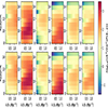 |
Fig. 13. Randomly selected examples of true (top) and emulated (bottom) LORELI signals qualitatively showing the resemblance between emulated and simulated spectra. |
4.2.1. Inference on mock data
LOREMU allows the generation of a 8 × 8 power spectrum in milliseconds and is therefore a suitable method for forward modeling in an MCMC inference pipeline. Figure 14 shows examples of Bayesian inference on a simulated spectrum3, assuming perfect foreground removal and noise corresponding to a 100 h SKA observation, as explained previously. The inferences were performed using the EMCEE Python package (Foreman-Mackey et al. 2013). The log-likelihood of a model y with astrophysical parameter set θ, with respect to data x, and with total variance σtot, can be explicitly written:
 (14)
(14)
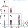 |
Fig. 14. Results of multiple inferences done using several versions of LOREMU, trained with different weight initializations (dashed). On the 2D panels, only the 1σ contours are shown for clarity. The blue dotted lines are the posteriors obtained using each emulator. The thick red line shows the posterior obtained using the average emulator on the noised signal, while the inference on the noiseless signal is shown in black. |
It is worth noting that this form of the likelihood assumes that Fourier modes are independent variables, an assumption discussed in Prelogović & Mesinger (2023) for example. While these latter authors show that using a diagonal covariance for the cosmic variance can lead to biased inference results, they also show that the nondiagonal terms are mostly erased by the level of their thermal noise, which is an order of magnitude below that used in our work. Therefore, we expect no significant contribution from these nondiagonal terms in our case. In our case, σtot is
 (15)
(15)
and includes, at each bin of k, z, the cosmic variance σCV, the variance of the SKA thermal noise σthermal, and the “training variance” σtrain, which represents the variance in the training of the network and is detailed below.
According to Bayes theorem, the posterior distribution of the parameters can be written:
 (16)
(16)
where π(θ) is the prior over the astrophysical parameters.
In order to estimate the error induced by an imperfect training of the emulator, nine different versions of LOREMU were trained. Each version uses the same architecture, and was trained using different weight initialization and with different random splits of the data to constitute the test and training sets. The rest of the training pipeline was kept unchanged. Each one of these trained emulators was subsequently used as the forward simulator in the MCMC pipeline, producing the different posteriors of Fig. 14. The inferences were done using 160 walkers, randomly initialized in the prior, and approximately 800 000 total steps. The prior on the astrophysical parameters is flat within the region in parameter space explored in LORELI and zero outside this region.
The inferences were all performed on the same simulated signal noised with the same 100 h SKA noise realisation, and therefore the differences between inferences are due to the different weight initializations and training stochasticity between the different versions of LOREMU. This training variance can be defined at each k, z, and astrophysical parameters set θ as
 (17)
(17)
where Ptarget and Ppredicted are the training spectra and the outputs of the emulator, respectively, and the sum is taken over a large number N of emulators trained with different weight initializations. Rigorously evaluating this variance would not only require a large number of emulators, but also a target signal for any value of θ, while we have signals only for the parameter values present in the LoReLi database. To address those difficulties, we chose to average this quantity over θ. The result is an approximation of the training variance. However, this is justified by the fact that the error shows no clear dependency on parameters. This variance adds a bias in the inference with single emulators, and putting the training variance in the likelihood widens the confidence contours. While negligible for fX, the effect of this training variance is comparable to that of the SKA 100 h thermal noise for the SFR parameters. In an attempt to marginalize over the random initializations, Fig. 14 shows a posterior obtained using the average predictions of the nine emulators in the MCMC framework, following the bagging method commonly used in machine learning. In order to demonstrate that, for the average emulator, the biases of the predictions are negligible compared to the uncertainty induced by the noise, Fig. 14 also shows the posterior applied to the noiseless signal (but with the SKA 100 h thermal noise variance still included in the likelihood). We see that, in this case, the confidence contours are well centered on the target parameter values. This also indicates that our inference results are only weakly affected by our choice of using a diagonal covariance in the likelihood.
τ and Mmin are unsurprisingly strongly anticorrelated, as their effects on star formation are degenerate. Similarly, fX is correlated with Mmin and anticorrelated with τ, as X-ray emissivity is proportional to SFR. We note that these effects are unlikely to stem from our choice of priors, because they are visible in confidence contours far away from the flat prior boundaries. Additionally, fesc is the least strongly constrained parameter, with large contours and non-negligible likelihood over the whole prior. Except for fesc, the true values of the astrophysical parameters are within the 1σ contours obtained after inference with the average emulator.
4.2.2. Inference on recent HERA data
In the previous section, we validated our method by applying it to mock observations generated from our simulated data. We now turn to real data, and provide an analysis of the most recent HERA observations (Abdurashidova et al. 2023), at z = 10.4 and z = 7.9. As indicated in Fig. 11, the most recent HERA upper limits are currently the only ones capable of constraining our data set. We follow the procedure detailed in Abdurashidova et al. (2022; thereafter HERA2022), which we briefly summarize here. The observed data are assumed to be the 21 cm signal, to which systematic uncertainties (typically foreground residuals and radio frequency interference) are added. The power of the systematic uncertainties is supposed to be positive, and marginalizing over them yields the likelihood:
![Mathematical equation: $$ \begin{aligned} L({ y} | \theta ) = \prod _{k,z} \frac{1}{2} \left[ 1 + \mathrm{erf} \left( \frac{x(k,z) - { y}(\theta , k ,z )}{\sqrt{2}\sigma (k,z)}\right) \right]. \end{aligned} $$](/articles/aa/full_html/2024/03/aa47591-23/aa47591-23-eq23.gif) (18)
(18)
The emulator was not retrained on spectra calculated with the k bins of HERA data with its window function. The posterior distribution of the astrophysical parameters obtained through MCMC inference is shown in Fig. 15. The only parameter for which the posterior distribution is different from its prior is fX. Qualitatively, our conclusions match those of HERA2022: a cold reionization of the Universe is an unlikely scenario. However, quantitatively, the constraints we put on fX appear looser than in HERA2022. In Fig. 6 of HERA2022, which shows the inference results as obtained using 21CMFAST, the likelihood decreases for fx < 1, while we only observe such a decrease for fX < 0.5. This may stem from a difference in the prior on the SFR parameters. Indeed, the observational constraints on SFR applied to LORELI and 21CMFAST only exist at z ≤ 10, leaving the functional form of the SFR evolution completely free at higher redshift. Different posteriors can result from this, as seminumerical codes typically assume that stars are formed instantaneously as some fraction of the collapsed gas. As detailed in Sect. 2, in LICORICE, the stellar fraction evolves with time. If the stellar fraction in LICORICE is typically lower than in seminumerical codes at high redshift and higher at lower redshift in order to be consistent with the same observational constraints on SFRD, then this difference in the inference result is expected. Unfortunately, as the codes function in significantly different ways with different parametrizations, understanding the difference in the predicted posteriors of both inferences would require an in-depth comparison of LICORICE and 21CMFAST (as well as with other codes) that does not yet exist and lies beyond the scope of this work. Regarding Fig. 14 of HERA2022, which was obtained using the seminumerical code described in HERA2022, an additional explanation may be that the authors marginalize over fr, a parameter that controls the intensity of an exotic radio background, while we implicitly fix fr to zero as the only background we consider is the CMB.
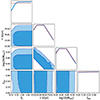 |
Fig. 15. Results of inference on HERA data using LOREMU. On the 1D panels, the priors are in red and the posteriors in blue. Contours represent 68% and 95% levels of confidence. |
As a final note, the inference was also attempted on upper limits from LOFAR (Mertens et al. 2020) using the exact same methodology. As could be expected from Fig. 11, no difference between priors and posteriors could be established in that case.
5. Conclusions
In this work, we present new functionalities of the LICORICE simulation code that allow low-resolution simulations of the EoR that reproduce many features of high-resolution simulations. These new functionalities are twofold. One is an implementation of the conditional mass function formalism as a way to statistically estimate the mass of unresolved dark matter halos. We then include the gas contained in these halos to compute star formation in low-resolution simulations, which would otherwise be severely underestimated. Using the Sheth-Tormen formulation of the CMF, we find excellent agreement with 10243 and 20483 simulations.
The other modification is a calculation of the temperature of the neutral phase of each particle. Due to poorly resolved ionization fronts in low-resolution simulations, we find that using the phase-averaged temperature of the particles leads to a significant overestimate of the intensity of the 21 cm signal. Using the neutral phase temperature leads to good agreement between results at low and high resolution.
Together, these improvements allow physically reasonable LICORICE simulations at 2563 resolution that run in approximately 300 cpuh. Consequently, this makes running many LICORICE simulations computationally feasible. Therefore, we present LORELI, a growing dataset of 760 LICORICE simulations with 2563 particles in 300 Mpc boxes. Full particle data are saved at 32 redshift values, and LORELI spans a four-parameter space: the escape fraction fesc, post, the X-ray emissivity fX, the minimum mass of star forming halos Mmin, and the gas-to-star conversion timescale τ. The latter two parameters were calibrated using constraints on the SFRD, and the first was chosen so that reionization ends in all models at between z ∼ 5 and z ∼ 8. LORELI therefore contains a variety of standard models of the EoR.
In the first application of this dataset, we summarize our data into independent power spectra values at 8 k and 8 z values. We then present LOREMU, a neural network trained on LORELI to produce accurate LICORICE power spectra given k, z, and a set of the four astrophysical parameters. During training, LOREMU reaches between ∼5% and 10% relative mean squared error averaged over the dataset. We then perform Bayesian inference using LOREMU and MCMC on a power spectrum generated using LICORICE, to which a noise realization corresponding to 100 h of SKA observations was added. Because different random weight initializations affect the result of the network training, nine different versions of LOREMU were trained, and training variance was included into the inference likelihood. By averaging the outputs of the different networks during inference, we obtain accurate posterior distributions. We find that this approach produces a posterior with very little bias by performing inference on a noiseless simulated signal. Finally, we apply the same inference pipeline to the most recent HERA upper limits and obtain constraints on lower values of fX, indicating that our Universe is unlikely to have followed a cold reionization scenario.
The new implementation of LICORICE suffers from some limitations. While star formation in resolved halos is sensitive to the local environment through the dynamics of the gas, unresolved halos of a given mass have a similar SFR, which only varies if they are located in particles with different stellar fractions. Moreover, the CMF formalism provides the cosmic average of the halo population in a given region with fixed overdensity. In reality, such regions may present fluctuations around this average. A future improvement will be to include stochasticity in the unresolved SFR, both from the halo population fluctuations and from the star formation efficiency of each unresolved halo. The latter will have to be parameterized with one last additional astrophysical parameter. Future versions of the LORELI database will include both a denser sampling of the parameter space and variations of additional astrophysical parameters.
In this work, we have only begun to tap the potential of the LORELI database. As we are modeling the 21 cm signal using full nonlinear dynamics and 3D radiative transfer, we can hope that the non-Gaussian properties of the signal are well accounted for. It will be relevant to explore inference based on non-Gaussian summary statistics of the signal. An explicit likelihood is usually not available in this case. One solution is to choose summary statistics that, while encoding non-Gaussian properties of the signal, have themselves near-Gaussian behaviors (due to the central limit theorem) and model the likelihood as a multivariate Gaussian. Another promising avenue is to use simulation-based inference (e.g., Zhao et al. 2022). We will be working toward both goals.
Available at https://21ssd.obspm.fr/
The detailed signification of the technical terms can be found at https://keras.io/
Calculated using the following astrophysical parameters: fX = 0.56, τ = 27 Gyr, Mmin = 109.06 M⊙, fesc, post = 0.2.
Acknowledgments
This project was provided with computer and storage resources by GENCI at TGCC thanks to the grant 2023-A0130413759 on the supercomputer Joliot Curie’s ROME partition. This study was granted access to the HPC resources of MesoPSL financed by the Région Île-de-France and the project EquipMeso (reference ANR-10-EQPX-29-01) of the programme Investissements d’Avenir supervised by the Agence Nationale pour la Recherche.
References
- Abdurashidova, Z., Aguirre, J. E., Alexander, P., et al. 2022, ApJ, 924, 51 [NASA ADS] [CrossRef] [Google Scholar]
- Abdurashidova, T. H. C. Z., Adams, T., Aguirre, J. E., et al. 2023, ApJ, 945, 124 [NASA ADS] [CrossRef] [Google Scholar]
- Alsing, J., & Wandelt, B. 2018, MNRAS, 476, L60 [NASA ADS] [CrossRef] [Google Scholar]
- Alsing, J., Wandelt, B., & Feeney, S. 2018, MNRAS, 477, 2874 [NASA ADS] [CrossRef] [Google Scholar]
- Baek, S., Di Matteo, P., Semelin, B., Combes, F., & Revaz, Y. 2009, A&A, 495, 389 [NASA ADS] [CrossRef] [EDP Sciences] [Google Scholar]
- Baek, S., Semelin, B., Di Matteo, P., Revaz, Y., & Combes, F. 2010, A&A, 523, A4 [NASA ADS] [CrossRef] [EDP Sciences] [Google Scholar]
- Barkana, R. 2018, Nature, 555, 71 [Google Scholar]
- Bianco, M., Iliev, I. T., Ahn, K., et al. 2021, MNRAS, 504, 2443 [NASA ADS] [CrossRef] [Google Scholar]
- Bouwens, R. J., Illingworth, G. D., Oesch, P. A., et al. 2015, ApJ, 803, 1 [NASA ADS] [CrossRef] [Google Scholar]
- Bouwens, R. J., Aravena, M., Decarli, R., et al. 2016, ApJ, 833, 72 [NASA ADS] [CrossRef] [Google Scholar]
- Bowman, J. D., Rogers, A. E., Monsalve, R. A., Mozdzen, T. J., & Mahesh, N. 2018, Nature, 555, 67 [NASA ADS] [CrossRef] [Google Scholar]
- Chen, N., Doussot, A., Trac, H., & Cen, R. 2020, ApJ, 905, 132 [NASA ADS] [CrossRef] [Google Scholar]
- Chollet, F. 2015, https://keras.io [Google Scholar]
- Ciardi, B., Stoehr, F., & White, S. D. M. 2003, MNRAS, 343, 1101 [NASA ADS] [CrossRef] [Google Scholar]
- Cohen, A., Fialkov, A., Barkana, R., & Lotem, M. 2017, MNRAS, 472, 1915 [Google Scholar]
- Datta, K. K., Mellema, G., Mao, Y., et al. 2012, MNRAS, 424, 1877 [NASA ADS] [CrossRef] [Google Scholar]
- Datta, K. K., Jensen, H., Majumdar, S., et al. 2014, MNRAS, 442, 1491 [NASA ADS] [CrossRef] [Google Scholar]
- Davies, F. B., Hennawi, J. F., Bañados, E., et al. 2018, ApJ, 864, 142 [NASA ADS] [CrossRef] [Google Scholar]
- Doussot, A., & Semelin, B. 2022, A&A, 667, A118 [NASA ADS] [CrossRef] [EDP Sciences] [Google Scholar]
- Doussot, A., Eames, E., & Semelin, B. 2019, MNRAS, 490, 371 [NASA ADS] [CrossRef] [Google Scholar]
- Fan, X., Carilli, C. L., & Keating, B. 2006, ARA&A, 44, 415 [Google Scholar]
- Fialkov, A., & Barkana, R. 2019, MNRAS, 486, 1763 [NASA ADS] [CrossRef] [Google Scholar]
- Foreman-Mackey, D., Hogg, D. W., Lang, D., & Goodman, J. 2013, PASP, 125, 306 [Google Scholar]
- Furlanetto, S. R., Peng, Oh. S., & Briggs, F. H., 2006, Phys. Rep., 433, 181 [NASA ADS] [CrossRef] [Google Scholar]
- Ghara, R., Mellema, G., Giri, S. K., et al. 2018, MNRAS, 476, 1741 [NASA ADS] [CrossRef] [Google Scholar]
- Greig, B., & Mesinger, A. 2015, MNRAS, 449, 4246 [NASA ADS] [CrossRef] [Google Scholar]
- Greig, B., & Mesinger, A. 2018, MNRAS, 477, 3217 [NASA ADS] [CrossRef] [Google Scholar]
- Greig, B., Mesinger, A., & Bañados, E. 2019, MNRAS, 484, 5094 [NASA ADS] [CrossRef] [Google Scholar]
- Hahn, O., & Abel, T. 2011, MNRAS, 415, 2101 [Google Scholar]
- Jennings, W. D., Watkinson, C. A., Abdalla, F. B., & Mcewen, J. D. 2019, MNRAS, 483, 2907 [NASA ADS] [CrossRef] [Google Scholar]
- Kaurov, A. A., & Gnedin, N. Y. 2014, ApJ, 787, 146 [NASA ADS] [CrossRef] [Google Scholar]
- Kendall, A., & Gal, Y. 2017, Adv. Neural Inf. Proc. Syst., 2017, 5575 [Google Scholar]
- Krause, F., Thomas, R. M., Zaroubi, S., & Abdalla, F. B. 2018, New Astron., 64, 9 [NASA ADS] [CrossRef] [Google Scholar]
- Lacey, C., & Cole, S. 1993, MNRAS, 262, 627 [NASA ADS] [CrossRef] [Google Scholar]
- Lewis, J. S., Ocvirk, P., Sorce, J. G., et al. 2022, MNRAS, 516, 3389 [NASA ADS] [CrossRef] [Google Scholar]
- Mao, Y., Koda, J., Shapiro, P. R., et al. 2020, MNRAS, 491, 1600 [NASA ADS] [CrossRef] [Google Scholar]
- McLeod, D. J., McLure, R. J., & Dunlop, J. S. 2016, MNRAS, 459, 3812 [NASA ADS] [CrossRef] [Google Scholar]
- McQuinn, M., Zahn, O., Zaldarriaga, M., Hernquist, L., & Furlanetto, S. R. 2006, ApJ, 653, 815 [NASA ADS] [CrossRef] [Google Scholar]
- Mellema, G., Iliev, I. T., Alvarez, M. A., & Shapiro, P. R. 2006, New Astron., 11, 374 [NASA ADS] [CrossRef] [Google Scholar]
- Mertens, F. G., Mevius, M., Koopmans, L. V. E., et al. 2020, MNRAS, 493, 1662 [Google Scholar]
- Mesinger, A., & Furlanetto, S. 2007, ApJ, 669, 663 [Google Scholar]
- Mesinger, A., Furlanetto, S., & Cen, R. 2011, MNRAS, 411, 955 [Google Scholar]
- Mitra, S., Choudhury, T. R., & Ferrara, A. 2011, MNRAS, 413, 1569 [NASA ADS] [CrossRef] [Google Scholar]
- Monaghan, J. 1992, ARA&A, 97, 101 [Google Scholar]
- Murray, S., Greig, B., Mesinger, A., et al. 2020, J. Open Source Software, 5, 2582 [NASA ADS] [CrossRef] [Google Scholar]
- Neutsch, S., Heneka, C., & Brüggen, M. 2022, MNRAS, 511, 3446 [NASA ADS] [CrossRef] [Google Scholar]
- Ocvirk, P., Aubert, D., Sorce, J. G., et al. 2020, MNRAS, 496, 4087 [NASA ADS] [CrossRef] [Google Scholar]
- Oesch, P. A., Bouwens, R. J., Illingworth, G. D., Labbé, I., & Stefanon, M. 2018, ApJ, 855, 105 [Google Scholar]
- Patil, A. H., Yatawatta, S., Koopmans, L. V. E., et al. 2017, ApJ, 838, 65 [NASA ADS] [CrossRef] [Google Scholar]
- Planck Collaboration VI. 2020, A&A, 641, A6 [NASA ADS] [CrossRef] [EDP Sciences] [Google Scholar]
- Planck Collaboration XIII. 2016, A&A, 594, A13 [NASA ADS] [CrossRef] [EDP Sciences] [Google Scholar]
- Prelogović, D., & Mesinger, A. 2023, MNRAS, 524, 4239 [CrossRef] [Google Scholar]
- Reed, D. S., Bower, R., Frenk, C. S., Jenkins, A., & Theuns, T. 2007, MNRAS, 374, 2 [NASA ADS] [CrossRef] [Google Scholar]
- Reis, I., Fialkov, A., & Barkana, R. 2021, MNRAS, 506, 5479 [NASA ADS] [CrossRef] [Google Scholar]
- Ross, H. E., Dixon, K. L., Iliev, I. T., & Mellema, G. 2017, MNRAS, 468, 3785 [NASA ADS] [CrossRef] [Google Scholar]
- Rubiño-Martín, J. A., Betancort-Rijo, J., & Patiri, S. G. 2008, MNRAS, 386, 2181 [CrossRef] [Google Scholar]
- Santos, M. G., Ferramacho, L., Silva, M. B., Amblard, A., & Cooray, A. 2010, MNRAS, 406, 2421 [NASA ADS] [CrossRef] [Google Scholar]
- Schaeffer, T., Giri, S. K., & Schneider, A. 2023, MNRAS, 526, 2942 [NASA ADS] [CrossRef] [Google Scholar]
- Schmit, C. J., & Pritchard, J. R. 2018, MNRAS, 475, 1213 [NASA ADS] [CrossRef] [Google Scholar]
- Semelin, B. 2016, MNRAS, 455, 962 [NASA ADS] [CrossRef] [Google Scholar]
- Semelin, B., Combes, F., & Baek, S. 2007, A&A, 474, 365 [NASA ADS] [CrossRef] [EDP Sciences] [Google Scholar]
- Semelin, B., Eames, E., Bolgar, F., & Caillat, M. 2017, MNRAS, 472, 4508 [NASA ADS] [CrossRef] [Google Scholar]
- Semelin, B., Mériot, R., Mertens, F., et al. 2023, A&A, 672, A162 [NASA ADS] [CrossRef] [EDP Sciences] [Google Scholar]
- Sheth, R. K., Mo, H. J., & Tormen, G. 2001, MNRAS, 323, 1 [NASA ADS] [CrossRef] [Google Scholar]
- Shimabukuro, H., & Semelin, B. 2017, MNRAS, 468, 3869 [NASA ADS] [CrossRef] [Google Scholar]
- Singh, S., Nambissan, T. J., Subrahmanyan, R., et al. 2022, Nat. Astron., 6, 607 [NASA ADS] [CrossRef] [Google Scholar]
- Springel, V., Yoshida, N., & White, S. D. 2001, New Astron., 6, 79 [Google Scholar]
- Tramonte, D., Rubiño-Martín, J. A., Betancort-Rijo, J., & Dalla Vecchia, C. 2017, MNRAS, 467, 3424 [NASA ADS] [CrossRef] [Google Scholar]
- Trott, C. M., Jordan, C. H., Midgley, S., et al. 2020, MNRAS, 493, 4711 [NASA ADS] [CrossRef] [Google Scholar]
- Wang, F., Davies, F. B., Yang, J., et al. 2020, ApJ, 896, 23 [NASA ADS] [CrossRef] [Google Scholar]
- Wouthuysen, S. A. 1952, Physica, 18, 75 [NASA ADS] [CrossRef] [Google Scholar]
- Zhao, X., Mao, Y., Cheng, C., & Wandelt, B. D. 2022, ApJ, 926, 151 [NASA ADS] [CrossRef] [Google Scholar]
All Tables
All Figures
|
Fig. 1. Evolution with redshift of the halo mass function of HIRRAH-21, calculated using a FoF algorithm. We also show the history of theoretical PS and ST HMFs for the same cosmology. |
| In the text | |
|
Fig. 2. Evolution of the simulated CMF with the overdensity δ and of the theoretical CMFs as predicted by the ST and EPS models. In order to match the high-resolution simulation, the σ in the EPS model has been scaled up by 5% on average. |
| In the text | |
|
Fig. 3. History of the SFR of HIRRAH-21 and LORRAH-21. As a reference, observational data from Bouwens et al. (2016), Oesch et al. (2018), McLeod et al. (2016) are included. The SFRD of a 10243 particles simulation is also plotted, and is consistent with that of a LORRAH-21 simulation using a Mmin parameter set at the value of the smallest resolved halos in the 10243 simulation. |
| In the text | |
|
Fig. 4. History of the average temperature of all particles in both LORRAH-21 and HIRRAH-21, as well as the temperature of weakly (< 2%) ionized particles. In the case of LORRAH-21, the temperature of the neutral phase of the particles is also shown. |
| In the text | |
|
Fig. 5. Global 21 cm signal in HIRRAH-21 and LORRAH-21, the latter calculated using either the phase-averaged temperature ⟨T⟩ of particles or the temperature of their neutral phase THI. This shows that properly taking into account the temperature of the neutral phase is critical in order to correctly model the 21 cm signal in low-resolution numerical simulations. |
| In the text | |
|
Fig. 6. Star formation rate density history for the 17 (τ, Mmin) parameter couples used in LORELI simulations (solid). The parameters were selected from a grid after a χ2 goodness-of-fit test. Only the parameter couples yielding a p-value p such that 1 − p < 0.95 for at least one of the plotted observational data sets were kept from the initial grid. For reference, the SFR in HIRRAH-21 is also plotted (dashed). |
| In the text | |
|
Fig. 7. Thomson optical depth of the LORELI signals. The ionization histories of the simulations confine the optical depths to within 1σ of Planck’s 2015 measurement (dotted: central value, shaded region: 1σ). As in 21SSD (Semelin et al. 2017), the second ionization of He is assumed to occur at z = 3. |
| In the text | |
|
Fig. 8. Average ionization fraction of the LORELI models, as well as observations from Bouwens et al. (2015), Davies et al. (2018), Wang et al. (2020). These observations were not used to calibrate the database, and reionization ends in all models between z ∼ 8 and z ∼ 5. |
| In the text | |
|
Fig. 9. Global 21 cm brightness temperature of the LORELI simulations. As opposed to 21SSD, global brightness temperatures are calculated from full 3D snapshots, not single slices of lightcones, and therefore do not exhibit small redshift-scale fluctuations. Color represents the value of fX, the parameter which impacts the depth of the signal the most. |
| In the text | |
|
Fig. 10. Power spectra of the LORELI simulations at k = 0.1 h/cMpc as a function of z. These are compared to recent upper limits of various instruments (Patil et al. 2017; Mertens et al. 2020; Trott et al. 2020; Abdurashidova et al. 2023) as well as theoretical thermal noise power of 1000 h observations with NenuFAR and LOFAR. |
| In the text | |
|
Fig. 11. Power spectra of LORELI models as a function of k at redshifts of 9, 11, and 14, from top to bottom. The value of the SKA thermal noise (1000 h of observation) is plotted to demonstrate that the LORELI signals should be detectable by the instrument. |
| In the text | |
|
Fig. 12. Diagnostics of the performance of the emulator. Top left: At each k, z, median across the dataset of the emulator error-to-thermal-noise ratio. Top right: At each k, z, median across the dataset of the emulator error-to-cosmic-variance ratio. The error increases with cosmic variance, as the deterministic network cannot replicate the noise induced by cosmic variance. Bottom left: 100x mean squared relative error across the dataset between the emulator prediction and the training sample. Bottom right: Loss at each k, z. Faint signal at high z causes low loss but high relative error. Cosmic variance causes high loss and relative error at low k. Additionally, we checked that the mean square relative error exhibits no systematic trend depending on the values of the astrophysical parameters. |
| In the text | |
|
Fig. 13. Randomly selected examples of true (top) and emulated (bottom) LORELI signals qualitatively showing the resemblance between emulated and simulated spectra. |
| In the text | |
|
Fig. 14. Results of multiple inferences done using several versions of LOREMU, trained with different weight initializations (dashed). On the 2D panels, only the 1σ contours are shown for clarity. The blue dotted lines are the posteriors obtained using each emulator. The thick red line shows the posterior obtained using the average emulator on the noised signal, while the inference on the noiseless signal is shown in black. |
| In the text | |
|
Fig. 15. Results of inference on HERA data using LOREMU. On the 1D panels, the priors are in red and the posteriors in blue. Contours represent 68% and 95% levels of confidence. |
| In the text | |
Current usage metrics show cumulative count of Article Views (full-text article views including HTML views, PDF and ePub downloads, according to the available data) and Abstracts Views on Vision4Press platform.
Data correspond to usage on the plateform after 2015. The current usage metrics is available 48-96 hours after online publication and is updated daily on week days.
Initial download of the metrics may take a while.