| Issue |
A&A
Volume 698, June 2025
|
|
|---|---|---|
| Article Number | A80 | |
| Number of page(s) | 17 | |
| Section | Cosmology (including clusters of galaxies) | |
| DOI | https://doi.org/10.1051/0004-6361/202452901 | |
| Published online | 29 May 2025 | |
Comparison of Bayesian inference methods using the LORELI II database of hydro-radiative simulations of the 21-cm signal
1
Observatoire de Paris, PSL Research University, Sorbonne Université, CNRS, LERMA, 75014 Paris, France
2
Department of Physics, Imperial College London, Blackett Laboratory, Prince Consort Road, London SW7 2AZ, UK
⋆ Corresponding author.
Received:
6
November
2024
Accepted:
24
March
2025
Abstract
While the observation of the 21-cm signal from the cosmic dawn and epoch of reionisation is an instrumental challenge, the interpretation of a prospective detection is still open to questions regarding the modelling of the signal and the Bayesian inference techniques that bridge the gap between theory and observations. To address some of these questions, we present LORELI II, a database of nearly 10 000 simulations of the 21-cm signal run with the Licorice 3D radiative transfer code. With LORELI II, we explored a five-dimensional astrophysical parameter space where star formation, X-ray emissions, and UV emissions are varied. We then used this database to train neural networks and perform Bayesian inference on 21-cm power spectra affected by thermal noise at the level of 100 hours of observation with the Square Kilometre Array. We studied and compared three inference techniques: an emulator of the power spectrum, a neural density estimator that fits the implicit likelihood of the model, and a Bayesian neural network that directly fits the posterior distribution. We measured the performance of each method by comparing them on a statistically representative set of inferences, notably using the principles of simulation-based calibration. We report errors on the 1D marginalised posteriors (biases and over or under confidence) below 15% of the standard deviation for the emulator and below 25% for the other methods. We conclude that at our noise level and our sampling density of the parameter space, an explicit Gaussian likelihood is sufficient. This may not be the case at a lower noise level or if a denser sampling is used to reach higher accuracy. We then applied the emulator method to recent HERA upper limits and report weak constraints on the X-ray emissivity parameter of our model.
Key words: methods: numerical / methods: statistical / dark ages / reionization / first stars
© The Authors 2025
 Open Access article, published by EDP Sciences, under the terms of the Creative Commons Attribution License (https://creativecommons.org/licenses/by/4.0), which permits unrestricted use, distribution, and reproduction in any medium, provided the original work is properly cited.
This article is published in open access under the Subscribe to Open model. This email address is being protected from spambots. You need JavaScript enabled to view it. to support open access publication.
1. Introduction
The 21-cm signal of neutral hydrogen is a promising probe of the early Universe. Emitted by the intergalactic medium (IGM), its features have been shaped by the properties of the first structures during the first billion years of the Universe. Indeed, as the first galaxies appeared during the so-called cosmic dawn (z ⪆ 20), they heated and ionised their surroundings. Due to the Wouthuysen-Field effect (Wouthuysen 1952; Field 1958), the spin temperature of neutral hydrogen leaves a state of equilibrium with the cosmic microwave background (CMB). Through the action of the local Lyman-α flux, the spin temperature becomes coupled with the local kinetic temperature. As a consequence, a contrast between the brightness temperature of the CMB and the 21-cm signal appears. This contrast depends on the local density of neutral Hydrogen and on its temperature and is therefore linked to the UV and X-ray emissions of the first galaxies (for a review, see e.g. Furlanetto & Pritehard 2006; Pritchard & Loeb 2012). Measuring the 21-cm signal would therefore allow astrophysicists to put tight constraints on the physical properties of the first sources of light, such as the minimum mass of star forming dark matter halos or the spectral emissivity of the galaxies in the UV and X-ray bands (e.g. Greig & Mesinger 2015; Abdurashidova et al. 2022).
Accessing this wealth of information remains an observational challenge. The SKA1 should be able to accurately measure the signal power spectrum and eventually provide a full 3D tomography of the 21-cm signal. In the meantime, current radio-interferometers (e.g. LOFAR2, NenuFAR3, HERA4, MWA5) are attempting to constrain the power spectrum of the signal and are reporting ever-tightening upper limits on this statistical quantity (e.g. Abdurashidova et al. 2022; Mertens et al. 2020; Munshi et al. 2024; Yoshiura et al. 2021). However, the 21-cm signal has been estimated to be around 104 times fainter than the foreground emission of nearby radio sources (e.g. Chapman & Jelić 2019). The foreground emissions from these sources must be modelled with extreme care before being subtracted from the observations, or altogether avoided, which then sacrifices part of the information in the process. Systematics of the instrument must also be mastered to bring the detection level to its theoretical limit, the thermal noise. In parallel, global signal experiments have tried to detect the average value of the 21-cm signal in the whole sky. EDGES6 reported a very deep signal (Bowman et al. 2018, ∼ − 500 mK at z ∼ 20), a result that subsequent experiments failed to reproduce (Singh et al. 2022) and that is not in the range of signals predicted with standard models of reionisation.
Producing accurate models of the 21-cm signal during the first billion years of the Universe is equally challenging. The physical processes at play couple scales across many orders of magnitude, forcing numerical setups to simulate ⪆ 300 Mpc boxes while taking into account galactic-scale phenomena. One also has to account for the propagation of UV and X-ray photons and their interaction with the IGM. To deal with this, the community has chosen a variety of approaches. The first is to use time-saving approximations whenever possible, which has resulted in a number of semi-analytical codes (see e.g. Sobacchi & Mesinger 2014; Reis et al. 2021). Those codes typically simulate the evolution of the dark matter density field, statistically estimate the population of dark matter halos in each resolution element and (crucially) bypass the actual simulation of the radiative transfer by estimating the size of ionised regions surrounding sources using photon budget arguments. This approach allows for a computation of a single 21-cm field in a couple CPU hours (cpuh) in typical setups. On the opposite side of the spectrum are fully numerical hydro-radiative simulations that, comparatively, are extremely computationally expensive, as these codes can require millions of cpuh to simulate a single box at high resolution. They are assumed to be more accurate, as they tend to rely on fewer approximations and more on first principle physics. They typically differentiate between the dynamics of dark matter and baryonic matter, resolve the relevant gravitationally bound structures, and perform 3D radiative transfer (e.g. Ciardi et al. 2003; Mellema et al. 2006; Mineo et al. 2011; Semelin et al. 2017; Ocvirk et al. 2020; Lewis et al. 2022; Doussot & Semelin 2022). Among these codes is Licorice, which is used in this work as well as in Meriot & Semelin (2024) (see also references therein). The community has also designed a few codes of intermediate cost, such as Schaeffer et al. (2023), Ghara et al. (2018), which typically ‘paint’ baryons over simulated dark matter density fields or halo catalogues, and solve spherically symmetric 1D radiative transfer to compute the 21-cm signal.
The interpretation of instrumental data using Bayesian inference typically requires tens or hundreds of thousands of realisations with different sets of astrophysical parameters and, ideally, many realisations of the density field at each point in parameter space. This makes the method computationally intractable for codes that take more than a few cpuh to simulate the epoch of reionisation (EoR). For this reason, semi-analytical codes have been widely used to develop data processing and inference pipelines. However, in a previous work (Meriot & Semelin 2024), we presented LORELI I, a database of 760 moderate-resolution 3D radiative transfer simulations of the EoR suited for inference purposes.
The most common inference technique used by the community is the classical Markov Chain Monte Carlo (MCMC) approach. While its convergence towards the true posterior distribution is guaranteed, it suffers from two caveats. First, it requires an explicitly written likelihood, which in general does not exist for 21-cm summary statistics and exists only in an approximate form for the 21-cm power spectrum. Second, it requires the simulations to be run sequentially during the inference process and not upfront. Performing inference on n different observed datasets requires n times the computation cost needed for one dataset, and the process is said to be ‘non-amortised’. In practice, the technique is only suitable for the fastest codes. This has led the community to explore alternative methods based on machine learning. For instance, one approach consists of performing simulation-based inference (SBI). As opposed to the MCMC algorithm, SBI does not require an explicit likelihood; instead, it takes advantage of the fact that a result from the modelling pipeline (which typically includes the generation of the initial density field, simulation of the cosmological 21-cm signal, and modelling of the instrumental noise) is a draw in the likelihood inherent to the model. Given that the implicit likelihood defined by the model is not subject to approximations, that the only requirement for SBI is to be able to generate signals, and that the computation cost is upfront and amortised, this approach has received significant attention in the 21-cm community (see e.g. Papamakarios & Murray 2016; Alsing & Wandelt 2018; Alsing et al. 2019; Zhao et al. 2022a; Prelogović & Mesinger 2023). Different versions of SBI exist, and here we focus on training a neural density estimator (NDE) to fit the likelihood before using the fit in an MCMC pipeline, and training a Bayesian neural network (BNN) to estimate the posterior.
In this paper, we greatly expand on the work presented in Meriot & Semelin (2024). In Section 1, we present LORELI II, a database of 10 000 hydro-radiative numerical simulations of the EoR. In Section 2, we give details about the three machine learning-based inference techniques that we explore in this work, namely using an emulator of the simulation code in an MCMC pipeline, using a NDE to fit the true likelihood sampled by the training set, and using a BNN to directly predict the posterior. In Section 3, we present the performance of these inference methods and comment on their convergence.
2. The LORELI II database
2.1. The Licorice simulation code
Here we briefly summarise the features of the simulation code, and present the new version of the LORELI database. Licorice is an N-body hydro-radiative simulation code of the EoR. Dynamics of gas and dark matter particles is solved using a TREE+SPH7 approach (Appel 1985; Barnes & Hut 1986; Springel 2005). As detailed in Meriot & Semelin (2024), the conditional mass function (CMF) of each gas particle is calculated at every time step, following the extension of the Sheth-Tormen mass function (Sheth & Tormen 2002) presented in Rubiño-Martín et al. (2008). The CMF formalism gives a statistical estimate of the average number of unresolved dark matter halos in a given mass bin, in the region represented by a gas particle. After integrating the CMF between a minimum halo mass Mmin and the mass of the region, it is straightforward to obtain fcoll, the fraction of the mass of the region in collapsed structures i.e. dark matter halos. This quantity is directly used to compute df*, the fraction of stellar mass created in each particle at each dynamical time step, according to
 (1)
(1)
where dt is the duration of a dynamical time step, τSF a parameter of the model that represents the typical timescale over which collapsed gas is converted into stars, and f* the stellar fraction of a particle. Particles with non-zero f* are considered sources and emit photon packets in the UV and X-ray continuum. To solve radiative transfer, gas particles are dispatched on an adaptive grid. Photon packets propagate at the speed of light and deposit energy in the grid cells they encounter. The temperature and ionisation state of gas particles in these cells are then updated over radiative time steps that may be up to 10 000 smaller than the dynamical time steps. A two phase model of the particles has been adopted: both the average temperature and the temperature of the neutral phase of the particles are computed, as calculating the 21-cm signal of a region using its average temperature leads to an overestimate (see Meriot & Semelin 2024). UV photon packets propagate until they are completely absorbed, but in order to save computing power, hard X-rays (with an energy greater than  , and a mean free path larger than the size of the box) are added to a uniform background after they propagated over distances larger than a box length. The simulation runs until the box is 99% ionised.
The physical properties of the particles are then interpolated on a 2563 grid in a post-processing step. The Wouthuysen-Field coupling is computed on this grid using the semi-analytical code SPINTER (Semelin et al. 2023). This allows for a computation of the brightness temperature of the 21 cm signal δTb using the classical equation (e.g. Furlanetto et al. 2006) at redshift z:
![Mathematical equation: $$ \begin{aligned} \delta T_b&= 27. \, x_{HI}(1+\delta ) \left[ \frac{T_s - T_{\rm CMB}}{T_s} \right] \left[ 1 + \frac{dv_{||}/dr_{||}}{ H(z) } \right]^{-1} \nonumber \\&\quad \times \left[ \frac{1+z}{10}\right]^{1/2} \left[ \frac{\Omega _b}{0.044} \frac{h}{0.7} \right] \left[ \frac{\Omega _m}{0.27}\right]^{1/2} \, \mathrm {mK}, \end{aligned} $$](/articles/aa/full_html/2025/06/aa52901-24/aa52901-24-eq3.gif) (2)
(2)
where xHI is the local neutral hydrogen fraction in a grid cell, δ the local overdensity, H the Hubble parameter, dv||/dr|| the line-of-sight velocity gradient, TCMB the Cosmic Microwave Background temperature at redshift z, and Ts the spin temperature of neutral hydrogen. A complete description of the code can be found in Meriot & Semelin (2024) and references therein.
2.2. The LORELI II database
Expanding upon LORELI I, a database of 760 Licorice simulations presented in Meriot & Semelin (2024), we now present LORELI II, a set of 9828 simulations spanning a five-dimensional parameter space. Simulations were run in (300 Mpc)3 boxes with a 2563 resolution, with varying initial conditions. The cosmology was chosen to be consistent with Planck 2018 (Aghanim et al. 2020). The following parameters were varied:
-
The parameters of the subgrid star formation model: 42 pairs of τSF ∈ [7 Gyr, 105 Gyr] and Mmin ∈ [108 M⊙, 4 × 10⁹ M⊙] were selected (6 τSF values for each of the 7 Mmin values). They produce star formation rate (SFR) densities within 2σ of the observational data presented in Bouwens et al. (2016), Oesch et al. (2018), McLeod et al. (2016).
-
The escape fraction of UV radiation in particles with ⟨xHII⟩> 3%: fesc, post ∈ {0.05, 0.275, 0.5}. In particles with ⟨xHII⟩< 3%, the escape fraction is kept at 0.003.
-
The X-ray production efficiency fX: 13 logarithmically spaced values in [0.1, 10]. this parameter controls the X-ray luminosities of source particles according to
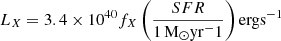 (e.g. Furlanetto et al. 2006)
 -
The ratio between hard (> 2 keV) and soft (< 2 keV) X-ray rH/S: 6 linearly spaced values in [0, 1]. rH/S is the ratio of energy emitted by X-ray binaries to the total energy emitted in X-rays:
In this setup, all simulations end between z ≲ 8 and z ≳ 4.5, and all simulations have Thomson optical depths within 3σ of Planck 2018 values, as shown in Fig. 1. Similarly to LORELI I, LORELI II was initially calibrated on star formation observations. However, a combination of factors acting in opposite directions have skewed this calibration while mostly preserving the most important ingredient for the 21-cm signal: the cosmic emissivity of galaxies. Consequently, we present a comparison of the luminosity functions in LORELI to observed ones on Fig. 2. They were obtained in a post-processing step and we assumed the same SFR-to-halo-mass power-law index α = 5/3 as was found in the CODA II simulation (see Ocvirk et al. 2020). The simulated luminosity functions show an acceptable agreement with observed ones, although they on average lay slightly below z ∼ 6 constraints at MAB1600 ≳ −20, suggesting that the source model and star formation algorithm of Licorice may have to be updated in the future. Naturally, the validity of the inference methods presented in this paper is insensitive to the uncertainties regarding the modelling of the luminosity functions or the low redshift disagreement, as all targets of inference are simulated (except for Section 5, in which HERA measurements are used at redshifts where the luminosity functions match observations).
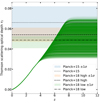 |
Fig. 1. Thomson scattering optical depth of the LORELI II simulations. Measurements by Planck 2015 and 2018 are also reported (Aghanim et al. 2020; Ade et al. 2016). The LORELI simulations are within 3σ of these constraints, although they were not used to calibrate the database per se. |
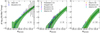 |
Fig. 2. UV luminosity functions of the LORELI II simulations at z ∼ 6, 8, 10. The dark green region shows, for each magnitude bin, where the middle 50% of the simulations lie, while the light green region shows where all simulations lie. We compare the simulated results with observations from Finkelstein et al. (2015), Oesch et al. (2018), Ishigaki et al. (2018), Atek et al. (2018), Bouwens et al. (2021, 2023). |
The particle data have been saved at ≈50 redshifts between z ≈ 60 and the end of reionisation, resulting in approximately 1 PB of data. Another 0.5 PB consist in post-processed data, namely 3D grids of UV luminosities, Wouthuysen-Field coupling, ionisation state, 21-cm brightness temperature, and its power spectrum. To illustrate the content of LORELI II, we show the global signals of LORELI II on Fig. 3. Most of the absorption features peak noticeably later than in some other models adopted by the 21-cm community (e.g. Bye et al. 2022; Breitman et al. 2024), which is most likely explained by the different star formation algorithms. For instance, our tests with Licorice showed that instantly converting collapsed gas into stars instead of doing so over time with Eq. (1) tends do noticeably shift the absorption peak to higher redshifts. The most intense signals reach ∼ − 220 mK at z ∼ 8, far from the EDGES measurement at −500 mK at z ∼ 16. The power spectra and global signals are publicly available8.
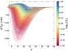 |
Fig. 3. Average global δTb of the 10 000 LORELI II simulations, colour-coded according to the X-ray intensity parameter fX. |
2.3. Sources of stochasticity
Several stochastic processes affect the 21-cm power spectra. The first one is the Cosmic Variance (CV, also called Sample Variance). Since a finite region of the sky is observed (or a finite volume is simulated), the larger the mode, the fewer times the power spectrum at that mode will be sampled. The measured value of the power spectrum will be an average of N samplings of the underlying expected spectrum, and the variance on that average decreases as N increases. While the small-scale modes will be extensively sampled and the resulting value will be very close to the theoretical average of the power spectrum, this introduces a significant uncertainty at large scales. Following McQuinn et al. (2006) we can compute the covariance matrix of the CV as
 (3)
(3)
where λ is the observed wavelength, A the area of a station, B = 10 MHz is the bandwidth, x the comoving distance to the observed redshift, y the depth of field. The other main source of stochasticity in this problem is naturally the thermal noise of the instrument. The detector noise covariance matrix is
 (4)
(4)
where Tsys is the system temperature and t the observation time. The standard deviation of the power spectrum caused by SKA thermal noise and CV is computed using a total covariance matrix C = CN + CCV as McQuinn et al. (2006):
![Mathematical equation: $$ \begin{aligned} \delta P_{21}(k,z) = \left[\sum _{|k| = k}\left( \frac{1}{ \frac{Ax^2 y }{\lambda (z)^2 B^2} C(\mathbf k ,\mathbf k ) } \right)^2 \right]^{-1/2}. \end{aligned} $$](/articles/aa/full_html/2025/06/aa52901-24/aa52901-24-eq8.gif) (5)
(5)
Technically, the Monte Carlo radiative transfer scheme in our simulation setup introduces an additional source of noise. However when using a reasonable number of photons (that depends on the numerical setup), it becomes negligible compared to the effect of the instrument. It must also be noted that, when we model a signal, the thermal noise and CV pose practical challenges of wildly different difficulties: at a given astrophysical parameter set θ, generating and then adding realisations of the thermal noise to a noiseless 21-cm signal is extremely fast, but exploring the range of results offered by cosmic variance requires running many simulations with different initial density field conditions. Due to computation and storage limitations, LORELI II contains only one such simulation at each point in parameter space.
2.4. The 21-cm power spectrum likelihood
The stochastic processes are critical in the inference problem, as they mean that the same observed spectrum can be generated by different, albeit close, points in parameter space, with different probabilities. The sources of stochasticity shape the likelihood and therefore the posterior.
A usual assumption is that the form of the likelihood is Gaussian:
 (6)
(6)
where y(θ) is a 21-cm power spectrum generated at θ and P21 the inference target. Here, Σ is the covariance matrix. Its diagonal represents the variance due to the aforementioned stochastic processes, and the off-diagonal terms imply coupling between modes induced by the complex physics of the 21-cm (e.g. the non-linear evolution of the density field as well as the heating and ionisation state of the IGM). Nonetheless, the covariance is sometimes assumed to be fully diagonal, yielding
 (7)
(7)
where σtot contains the diagonal of Σ. This last expression, although inaccurate, is convenient and easily evaluated, which makes it widely used (see Prelogović & Mesinger 2023, for a discussion).
In order to perform an accurate parameter inference using the LORELI simulations, two issues remain. One must be able to evaluate the likelihood at more points than the 10 000 simulated parameter sets of LORELI II. Typical classical inference requires ∼105 − 6 realisations for a 5D parameter space (Prelogović & Mesinger 2023; Abdurashidova et al. 2023). Some form of interpolation between the LORELI simulations is required. One would also benefit from relaxing the Gaussian Likelihood approximation. To do so, one must find a way to evaluate the true, unknown likelihood of the signal.
3. Inference methods
The previous sections laid the groundwork for the machine learning methods we use to perform the EoR parameter inference. In this section, we present three approaches that we apply to the 21-cm power spectrum. The first consists in emulating the power spectrum with a neural network and using the emulator in a classical MCMC framework, the second is a direct prediction of the posterior distribution of the astrophysical parameters with Bayesian Neural Networks, and the last works by fitting the likelihood of our data with a Neural Density Estimator. All implementations rely on Tensorflow9 and the Keras10 framework. In this section, we present and evaluate each inference method; we compare them in the next section.
3.1. Classical Markov chain Monte Carlo inference with an emulator
3.1.1. LorEMU
The emulator, named LorEMU II, is a network trained to take as inputs the astrophysical parameters of the LORELI II simulations and output the corresponding power spectra. The full architecture is shown in Table 1. It was trained on 8 × 8 power spectra, computed from coeval11 21-cm signal cubes at redshift z= [13.18, 12.06, 11.14, 10.37, 9.7, 9.13, 8.63, 8.18] and wavenumbers k= [0.16, 0.23, 0.33, 0.47, 0.66, 0.93, 1.32, 1.86] h/cMpc (thus we performed a multi-redshift inference). We find the spectra to be smooth at this resolution in redshift and wavenumbers and we use adjacent, non-overlapping k-bins, so we do not expect that a finer (k, z) grid would improve the results in the following.
Architecture and hyperparameters of LOREMU.
We first created a test set with 10% of the spectra, on which no network will train. Then, in the remaining 90%, another 10% random cut was done to form the validation set, while the training set comprises the rest. While the first cut was always the same, the second one changes between different initialisations of the networks. The logarithm of τSF, Mmin and fX is taken, and all input parameters were normalised between zero and one. The first version of LorEMU, trained on LORELI I, emulated the logarithm of the spectra. It was later found that training on the square root of the signal-to-noise ratio leads to more accurate results:
 (8)
(8)
Here σthermal is the standard deviation of the SKA thermal noise for 100 h of observations, given by Equations (4) and (5). This normalisation forces the network to learn the features that are observable by the instrument, and ignore those that are masked by the noise. This is not necessarily the case if the emulator simply predicts the spectra, as it may minimise its cost function by improving its performances in regions that would turn out to have a low signal-to-noise and will not be relevant during the inference. Additionally, the square root confines the signal-to-noise to a manageable dynamic range, leading in this case to better results than a log.
The training aimed at minimising a mean square error (MSE) loss with an RMSprop optimizer using a learning rate of 10−3 and convergence was typically reached after 500 epochs. Fig. 4 shows a few randomly selected examples of simulated and emulated spectra, to qualitatively assess the quality of the results.
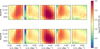 |
Fig. 4. Top: Randomly selected emulated power spectra. Bottom: Corresponding spectra from LORELI II. This figure is a simple illustration of the performances of LorEMU. |
Quantitatively, Fig. 5 shows different metrics to evaluate the performance of the network at each (k, z) bin, averaged over the test set. All quantities, except for the loss, have been computed on the signal-to-noise  (i.e. on denormalised signals, not on
  of Eq. (8)).
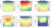 |
Fig. 5. Performance metrics of an instance of LorEMU, averaged over the test set. The network performs better where the CV and thermal noise are weak (see text for details). |
The top-left plot shows the MSE. It exhibits a strong dependence in k but not in z. The loss is the highest at large scales, where the cosmic variance is significant. This is detailed on the top-right plot, which shows the ratio of MSE and CV (for denormalised signals). At large scales, the ratio converges to ∼1, implying that the dominant factor of error is CV, and becomes negligible at small scales, where CV vanishes. Ideally, we want the emulator to learn the CV-averaged power spectrum at each point in the parameter space. In practice, our loss shows no sign of overfitting, and we observed poor performance at large scales on the training set, which indicates that the network does not learn the specific CV realisation that affects each signal in the dataset. Instead, it is hypothesised that it learns to average over the contribution of CV by smoothing out local fluctuations between points in the parameter space due to CV.
The loss and the root mean square error (RMSE) are minimal at high k, as indicated on the centre-left plot. However, the relative error at these scales is at its worst, as shown on the centre-right plot. These are regions in (k, z) where the thermal noise of the instrument is high, and the signal-to-noise consistently very low and easy to learn for the network. In regions of lower noise, where the emulator must be accurate in order to provide good inference results, the relative error shown on the mid-right plot is only a few % on average. Since we train the network to predict a spectrum unaffected by the thermal noise, the error can indeed become small compared to the noise. However, we cannot train it to predict spectra unaffected by CV because we have only one realisation at each parameter space point, and thus the error cannot become negligible compared to CV. Also, we have not observed any clear systematic dependence of the error level on the astrophysical parameters. The bottom-left plot of Fig. 5 shows the ratio of the absolute error and the thermal noise, while the bottom-right plot shows the mean square relative error. They confirm that the networks consistently perform best in the region most relevant for the inference.
Different metrics are exposed on Fig. 5, and they focus on different regions of (k, z), but in the 0.1 < k < 0.9 h.cMpc−1 range (i.e. in the low S/N region), the performances of LorEMU II are comparable with those of LorEMU I (trained on LORELI I, and studied in Meriot & Semelin 2024), in terms of mean square relative error (which describes a variance). They also typically outperform the emulator presented in Jennings et al. (2019) by a factor of ∼2.
In summary, the network performs best where the cosmic variance and the thermal noise is low. The relatively poor performances where there is noise and CV should be of minor consequence for the inferences, as this means that the network introduces errors where the sources of stochasticity already erase information about the physics of Reionisation and not where this information is available and clean.
3.1.2. Inference on mock data
LorEMU II can generate an 8 × 8 power spectrum in a few ms on an Nvidia T600 mobile GPU and can therefore reasonably be used in an MCMC pipeline. Let us perform a series of inferences on artificial data: a LORELI II signal, to which we can add a thermal noise realisation corresponding to 100 h of SKA observations. We assumed that the likelihood was given by Eq. (7). This assumption is challenged by, for example, Prelogović & Mesinger (2023), but this paper also shows that the off diagonal terms are mostly erased by the presence of thermal noise of 1000 h of observations, significantly weaker than in our setup. Next, we needed to specify the σtot that appears in the likelihood:
 (9)
(9)
We note that σthermal and σCV are given by Equations (3) to (5) and contain the standard deviation associated with the thermal noise and CV, respectively. The last term, σtrain, is caused by the imperfections of the emulator. For instance, the prediction of LorEMU depends on the random initialisation of its weights before training. Since the MSE of LorEMU is non-zero and does not show a strong dependency with the parameters θ, we followed the procedure outlined in Meriot & Semelin (2024) and considered that the emulated signal  is the corresponding simulated signal
  affected by a training noise, that is, a random perturbation of standard deviation σtrain given at each θ by:
 (10)
(10)
where N is a large number of emulators trained with different initialisations. Since  is only available at the parameter sets of LORELI II and not for any θ, and since the MSE of LorEMU does not strongly depend on θ, we estimated σtrain by averaging this quantity over θ.
Figure 6 shows the performance of a ‘stacked emulator’, i.e. measured using the average predictions of 10 different instances of LorEMU, trained with different weights initialisation and on different splits of the data to constitute the training and validation sets. Stacking the emulators results in an improvement of the performance and a decrease of the RMSE by a factor  . This is consistent with our hypothesis that the training error behaves as a random noise of mean zero, as it is the result expected from the central limit theorem. The relative absolute error of the stacked emulator is smaller than 5% across almost all k and z (when averaged over θ) and the absolute error is consistently significantly below the level of the thermal noise (≲5% for k ≳ 0.4 h.Mpc−1), as shown on the bottom-left panel. The average relative error consistently decreased compared to a single instance of LorEMU to reach 3% on average, and displays a smaller variance in the performances.
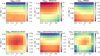 |
Fig. 6. Similar to 5 but for the average predictions of ten independently trained instances of LorEMU, leading to a significant performance improvement. For instance, the relative error typically decreases by a factor three. |
For an inference target, we used a simulated signal from LORELI II with the following parameters: Mmin = 108.8 M⊙, τSF = 25 Gyr, fX = 2.15, rH/S = 0.4, fesc = 0.275, near the centre of the LORELI II parameter space (our prior). In this section, we performed the inferences on a target signal unaffected by noise but with the effect of stochastic processes duly included in the inference frameworks. Since the signal was not affected by a noise realisation, we expected the posterior to be well centred around the true value of the parameters because we are in a situation where stochastic processes are mostly Gaussian. However, we note that, in the general case, a multi-dimensional posterior with a complex shape does not necessarily result in 1D marginalised posteriors centred on the true parameter values, even for a noiseless signal. The assessment of the results of the inferences in this section is heuristic, a formal validation is the object of the next section. Moreover, the target signal is still affected by a CV realisation, which may lead to a small bias in the posterior. Of course, an imperfect inference framework (emulator training in this case) should produce biases among other errors.
We ran the MCMC with each of the ten instances of LorEMU individually first, and then using the stacked emulator. The results are shown on Fig. 7. The resulting inference exhibits some variation depending on the actual emulator used, but the true values of the parameters always lie within the 68% confidence interval and the remaining bias is small compared to the 1σ (remember that here the target is a signal not affected by thermal noise, the largest source of stochasticity, but thermal does contribute to the posterior variance). Interestingly, all parameters are well constrained except for the escape fraction, which is common across all methods. It is possible that including the values of the power spectra at lower redshifts would allow better constraints.
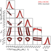 |
Fig. 7. Results of inference on a noiseless LORELI II power spectrum using ten independently trained versions of the LorEMU II emulator (red). The emulators show a non-negligible variance. This uncertainty can be mitigated by averaging the predictions of the different instances of LorEMU during the inference (black). On 2D posteriors, only the 1σ contours are shown, for clarity. |
For comparison, Figure 12 in Meriot & Semelin (2024) shows similar inferences performed using LorEMU I, on a signal from LORELI I. Qualitatively, the inferences on Fig. 7 done with LORELI II seem to exhibit less variance than those done with LORELI I. The inference obtained with the average prediction of 10 instances of LorEMU I seems also significantly more biased than what we observe with the average LorEMU II. This suggests that the architectural modifications to LorEMU II and the better sampling of LORELI II lead to better results compared to the work presented in Meriot & Semelin (2024).
Importantly, the posterior contains several points of the LORELI II grid within the 99% confidence regions. While not critical for the emulator, the other networks architectures described in the following need to train on signal affected by an instrumental noise realisation. Ensuring the sampling of the parameter space is dense enough to cause some overlap between the noised signal distributions of neighbouring points of the grid may help avoid a pathological regime where the networks learn to affect every noised versions of the same un-noised signal to the exact same parameter set with a very high probability instead of properly yielding the posterior or the likelihood. In other words, it should prevent the networks from becoming absurdly overconfident. The design of the LORELI II grid was motivated by the results obtained with LORELI I, and this inference tends to confirm that the database is suited for an inference on data affected by a noise at least as strong as the one on 100 h of SKA observations.
3.2. Simulation-based inference
In addition to the emulator, we explored in this work the use of SBI, also called likelihood-free inference. SBI relies on a simple fact: when repeatedly taking a given input θ (in our case, the astrophysical parameters), a simulation code will produce a distribution of outputs D. If the code is deterministic, this distribution is a Dirac, but in our case, the relevant output is a realistic mock observed 21-cm power spectrum which is affected by at least two sources of stochasticity: the thermal noise of the instrument and the cosmic variance. By definition, these outputs are drawn from P(D|θ), a likelihood function inherent in the simulation pipeline. If this likelihood function can be fitted and quickly evaluated, it can be used in a MCMC algorithm. An alternative is to directly fit the posterior. Different network architectures can also be used to fit the desired distribution.
As discussed in, for example, Prelogović & Mesinger (2024), using a Gaussian shape for the likelihood of the 21-cm power spectrum is an approximation, and this family of methods is in principle a way to relax it. For different variations and evaluations of their performance, see for instance Prelogović & Mesinger (2023), Zhao et al. (2022b), Saxena et al. (2023). In the following, we consider two approaches: we fit the posterior using a Bayesian Neural Network and fit the likelihood using a Neural Density Estimator.
3.3. Simulation-based inference with Bayesian neural networks: posterior estimation
First, we studied how to directly predict the posterior distribution of the astrophysical parameters using a Bayesian Neural Network. These networks contain so-called variational layers which differs from classic layers in the fact that the connections between neurons are not parametrised by single values for the weights but rather by weight distributions. When the layer is called, the input of the neurons are weighted by values drawn from these distributions. BNNs are probabilistic: repeatedly feeding them the same input will result in a distribution of outputs. For a review, the reader is redirected to Papadopoulou et al. (2016), Jospin et al. (2022). We note that Hortúa et al. (2020) presented a first, brief application (using dropout layers, not true weights distributions) of BNNs on the 21-cm signal. In the following, we expand on their work, in particular in terms of evaluation of the performance of the network. Let us first briefly summarize how BNNs work.
3.3.1. Variational inference
During training, given a dataset D = (x, y), one wishes for the parameters of the network to be adjusted so that the networks responds to an input x (in our case, a 21-cm power spectrum affected by a mock realisation of SKA noise) with an output close to y (the corresponding astrophysical parameters) with a high probability. That is, given some prior p(ω) set over the weights ω, one wishes to determine p(ω|D), the posterior distribution of the network’s weights given some data D. To do so, we naturally used the Bayes theorem:
 (11)
(11)
where  is the evidence. Calculating this integral (i.e. marginalising over the weights) is intractable except in the simplest cases. In practice, one turns to an approximation: the true posteriors p(ω|D) are replaced by parametrised distributions qϕ, characterised by some numerical parameters ϕ. A common choice, adopted in the following, is to set Gaussian distributions over the weights. As a note, classic layers with deterministic weights can be perceived as Dirac distributions in this formalism. To ensure that the qϕ are good approximations of the posterior, the ϕ parameters are tuned to minimise the Kullback-Leibler (KL) divergence between the true and approximated posteriors:
 (12)
(12)
This is equivalent to maximising the evidence lower bound (ELBO; Papadopoulou et al. 2016; Jospin et al. 2022):
 (13)
(13)
Architecture and hyperparameters of the BNN.
Maximising the first term means adjusting ϕ to maximise the likelihood. The second term acts as a regularisation term, that is, it penalises complex qϕ. This defines a minimisation objective: −LELBO. In theory, during a single epoch, in order to estimate −LELBO, a single example must be passed many times to properly sample the integrand. In practice, it is estimated by a single forward pass (Gal & Ghahramani 2016). This adds another source of noise to the training, but is assumed to converge properly in the limit of a large dataset. This leads to a discrete version of Eq. (13):
 (14)
(14)
where the sum is taken over the elements of the dataset. For each of them, a set of weights ωi is sampled from the layer distributions.
An additional feature of the BNN lies at its last layer. The BNN does not predict single values for the astrophysical parameters we wish to infer from the data. Instead, it predicts parameters of distributions. We chose to predict a mean vector μ and the full covariance matrix C that will capture the correlations between the astrophysical parameters. For instance, with one Gaussian component, the probability of the network outputting y given an input x and a set of weight values ω (sampled from the parametrised distributions sets over the weights) can be written as:
 (15)
(15)
This log-probability log p(y|x, ω) is the log p(D|ω) that appears in the loss function of Eq. (13).
3.3.2. Uncertainties with Bayesian neural networks
While the emulator-based approach requires an explicit prescription of each of the variances induced by all stochastic processes at play, the BNN does not, and can instead be used to produce an estimate of two forms of variance of interest. Indeed, after passing the same input x to the network N times, the model predicts a set of means {μn}1 ≤ n ≤ N and covariance matrices {Cn}1 ≤ n ≤ N. This allowed us to compute an estimate of the average prediction,
 (16)
(16)
as well as an estimate of the covariance of the model,
 (17)
(17)
In the last equation, the first sum characterises the aleatoric uncertainty, while the second sum is a measure of the epistemic uncertainty. The former is the uncertainty that arises from the noise inherent in the data (in this case, the instrumental noise and the cosmic variance), and the latter captures the variance caused by an imperfect training of the network, for instance due to a limited density of the training sample or insufficient optimisation. In this sense, what the epistemic uncertainty represents may be similar to the model error introduced in the explicit likelihood in the previous section.
The data on which the network trains is the power spectrum noised by instrumental effects, given in Section 2.3. To produce one realisation of the noise, one approach would be to draw values from a Gaussian distribution of mean 0 and a standard deviation given by Eq. (5). While this works in cases where the signal-to-noise is high, it leads to negative values where the noise is strong. These negative values are not physical, but would not impede the training if it were not for the need of normalisation. Indeed, the data must be normalised to an interval close to [0, 1] while maintaining the dynamic range i.e. having a network that learns the features of weak spectra just as well as strong ones. The negative values prevent the use of Eq. (8), or a logarithm. S-shaped functions like hyperbolic tangents or sigmoids may divide a set consisting of one power spectrum at one k, z affected by different noise realisations in two clusters depending on whether the noise added or subtracted power (i.e. it tends to create bimodal likelihoods). The network must then learn that these two clusters characterise the same data, which has empirically proven to be a challenge. A first solution is to cut negative values and replace them with some floor value such as 0, another is to compute the power spectra of noised δTb cubes and perform the inference on the power spectrum that includes the contribution of the noise. The latter would produce physically accurate results but is much more computationally intensive than the former. For now, we only use the first method.
The architecture of the network is shown on Table 2. While not heavier than the emulator, it is considerably harder to train, as the variational layers introduce a large amount of stochasticity in the training. On the upside, it acts as regularisation, and we never observed any sign of overfitting while training these networks.
Figure 8 shows, for the different values of the parameters, the aleatoric (left) and epistemic (right) errors, i.e. the average variances and variances of predicted means, computed on the validation set (without any instrumental noise). The means are comparatively extremely stable, which tends to show that the training sample is dense enough to constrain the weights of the network, and adding more data should only marginally improve the result. The predicted variances, which capture the noise in the data (i.e. the effect of CV and the thermal noise) are typically an order of magnitude above the epistemic error, and again typically larger than the parameter grid step, which should enable the network to generalise to signals generated using parameters sets not in LORELI II (but still inside the volume of parameter space sampled in the database). Interestingly, the variance exhibits a clear correlation with rH/S, a trend we weakly observe with the other methods. It could stem from the fact that a high rH/S delays and homogenises the heating, thus decreasing the signal-to-noise ratio.
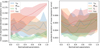 |
Fig. 8. Left: Mean standard deviation of the predicted distributions of each parameter by the BNN. For a single example, the mean was obtained by averaging the predicted means over 100 forward-passes (shown as solid lines), and the vertical width of the shaded regions show the dispersion of the results across the validation set. This quantifies the aleatoric uncertainty (i.e. the uncertainty caused by the noise in the data). Right: Standard deviation of the predicted means. This is the epistemic uncertainty (i.e. the error caused by the sparsity of the training sample). It is an order of magnitude smaller than the aleatoric uncertainty, indicating that the instrumental noise is the dominant source of variance. |
Figure 9 shows the means of the parameter distributions predicted by the BNN when applied to a noiseless signal compared to the true values of the parameters. Most (∼90,% see discussion in Sect. 4.1) lie on the y = x line. However, the network underperforms in many cases. First, the BNN tends to overestimate rH/S when the true value is 0, and tends to underestimate this parameter elsewhere. The network also has a tendency to underestimate Mmin and overestimate τSF (as it properly captures the correlation between the two), typically by 0.1, which is close to the parameter grid step.
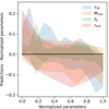 |
Fig. 9. Error of the BNN predictions. For each parameter, the shaded regions is centred on the difference between the average predicted mean and the true value, and the vertical width is given by the average standard deviation of the predicted distributions. While the predicted means are very stable (as shown on the right panel of Figure 8), the network shows a significant bias for all parameters save for fX in ∼10% of the cases. |
Like in the case of the emulator, we trained ten instances of the BNN with different weight initialisation. In this case, stacking the networks did not lead to a significant improvement of the results. The dispersion of the predictions decreases, but their average does not converge significantly towards the true values of the parameters. In other words, the error bars on Fig. 9 slightly decrease, but the points do not significantly get closer to the y = x line. This is not unexpected, since probabilistic networks are often perceived as a way to marginalise over a distribution of networks. As such, these approaches are less sensitive to their weight initialisations. However, this also means that the networks systematically converge during training towards weights that cause wrong predictions of the astrophysical parameters, as the errors displayed, for example, on Fig. 9 can be significant. This might suggest that the network is sensitive to cosmic variance or some unidentified outliers in the data.
Figure 10 shows the predictions of the 10 BNNs after forward-passing a noiseless signal 10 000 times, as well as the average posterior. The maxima of likelihood are slightly offset, a systematic bias that is not corrected by the stacking. The posterior on rH/S appears slightly bimodal, a feature missing when using the other inference methods. A comparison with the results of the other inference methods can be found in the next section.
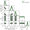 |
Fig. 10. Posteriors estimated by repeatedly forward passing a noiseless LICORICE power spectrum to ten independently trained BNNs (green) and to the stacked BNN (black). The results show little variance and seem to converge to slightly biased results. The posterior on rH/S shows a long tail not retrieved by the other inference methods. |
3.4. Simulation-based inference with neural density estimators: Likelihood fitting
We trained a NDE to fit the distribution of the data {Dn}1 ≤ n ≤ N given the astrophysical parameters {θn}1 ≤ n ≤ N, i.e. the likelihood of our physical model. To do so, one must choose an arbitrary functional form LNDE(D|θ) for the approximate likelihood, parametrised by the output of the NDE. The dataset to fit is the LORELI power spectra of the 21-cm signal, augmented by 100 realisations of the SKA thermal noise on the fly at each training epoch. As previously discussed, it would ideally contain several simulations per parameter set to sample cosmic variance, but this is not computationally feasible. Crucially, we used the same method to preprocess the spectra as with the Bayesian Neutral Networks.
The network is trained so that the parametrised likelihood fits the true likelihood LTrue of the model. Following Alsing et al. (2019), in theory, we want to minimise the KL divergence between the parametrised likelihood of the NDE and the true likelihood,
 (18)
(18)
minimising this KL is equivalent to minimising −∫LTrue(D|θ)log(LNDE(D|θ))dD, as we can only tune the parameters of LNDE. In practice, we do not know LTrue but our training set is composed of draws in LTrue, and minimising the KL divergence of the above equation is achieved by minimising the loss function,
 (19)
(19)
Once the network is trained to fit the true likelihood of the model, it can be put into an MCMC pipeline to perform the inference. Compared to the emulator-based method, this approach has the advantage of not requiring an explicit likelihood, it only requires a parametric functional form for the approximate likelihood that is flexible enough to fit the true likelihood with the desired accuracy. However, as is common with machine learning, a network made too flexible may be prone to overfitting. The functional form we chose for the parametrised likelihood is a multivariate Gaussian Mixture Model with η = 3 components, allowing the network to fit distributions more complex than the approximate Gaussian likelihood but with a manageable number of free parameters. As shown in Table 3, the network consists of a simple multilayer perceptron with three layers of 64 neurons each. Each parameter of the mixture model (i.e. the respective weights, means, diagonal terms and off diagonal terms of the Gaussian components) are predicted by an additional 64 neurons layer.
Architecture and hyperparameters of the NDE.
Training occurs over 35 epochs using an RMSprop optimizer and a learning rate of 2 × 10⁻³, and the training and validation losses show no sign of overfitting.
As before, we illustrate the method by performing an inference on a noiseless signal with 10 independently trained NDEs. The results are shown on Fig. 11. Again, we observe some variance of the maxima of likelihood, indicating a non-negligible training variance, but the true values of the parameters always lie well within the 68% confidence intervals. As an attempt to reduce this variance, the figure also shows another inference performed while stacking the NDEs, i.e. by using their averaged predictions for the log-likelihoods. This stacked NDE still seems to converge to a solution that is not perfectly centred around the true value of the parameters, a behaviour consistent with the one of the BNN. However, the dispersion of the result is reduced, and we will consider only the stacked NDE in the following.
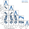 |
Fig. 11. Similar to 7 but for ten independently trained NDEs. They exhibit a similar amount of training variance as the emulators, but seem to display a larger systematic bias. |
4. Comparison between inference methods
We presented the 3 inference methods used in this work and showed inferences performed on the same signal as an illustration. We now wish to identify which method to use to interpret an eventual detection of the 21-cm power spectrum. To do so, we need to evaluate
-
their accuracy, i.e. whether the peak of the posterior distribution produced by an inference method is indeed the right one. In an ideal and simple setting, given that the noise is Gaussian distributed and of mean 0, inference on the average (equivalent to noiseless in this case) signal produced by a parameter set θ should yield a posterior that peaks at θ, the true values of parameters. This is true for simple cases and for a class of locally well-behaved models. We cannot guarantee that our model of the power spectrum belongs to that class, but the posteriors of the previous sections, as well as from other 21-cm inference works (e.g. Prelogović & Mesinger 2023; Zhao et al. 2022a; Greig & Mesinger 2018, 2015) do suggest that the posterior should peak at or near the true parameters. Effects like training variance and CV may create systematic bias and dispersion in the outcome of the inferences, but we expect them to be small.
-
their precision, i.e. we want to ensure that the posteriors we recover are not over- or underconfident. Following Cook et al. (2006) and Talts et al. (2018), we must check that posteriors obtained from noised signals stemming from θ should for instance contain θ 68% of the time in the 68% confidence contour, 95% of the time in the 95% confidence contour, etc. The best method is not necessarily the one that yields the most confident posterior.
4.1. A heuristic approach: Inference on noiseless signals
As a first element of comparison, Fig. 12 shows inferences using all three methods (using stacked networks). On this signal, the BNN appears slightly less confident than the other methods, and the NDE shows the most bias. However, the differences between maxima of likelihood are of the order of ∼0.5σ, similar to what can be found in works such as Prelogović & Mesinger (2023).
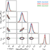 |
Fig. 12. Inference with all (stacked) networks. All three results agree to a large extent. The maxima of likelihood are close; they are all within 1σ of each other and within a grid step. Nonetheless, the BNN is systematically less confident than the others, while the predictions of NDE are slightly more biased. For clarity, we exclude fesc from the analysis, as it is systematically poorly reconstructed by all three methods. |
Naturally, a single inference is not enough to evaluate the performance of these methods. To provide a robust comparison, we performed inferences on 100 randomly selected noiseless signals. For each inference, we found the maximum of each 1D marginalised posterior and compute the bias δμ (the difference between the true values of the parameters and the values parameters where the posterior peaks) and the standard deviation σ of the 1D posteriors. Since what we expect from the networks is effectively to be able to interpolate between the signals of the database, a useful scale against which we can compare our error is the typical grid step of LORELI II, Δgrid = 0.089, 0.169, 0.088, 0.5, 0.2 for the normalised τSF, Mmin, fX, rH/S respectively. However, since the escape fraction fesc is systematically very poorly constrained, we focus on the other four parameters. We note that the fact that our models cannot discriminate between different values fesc may force them to learn to average over cosmic variance (at least to some extent), as they are presented with several power spectra affected by different realisation of CV but labelled by the same set of the meaningful parameters.
To evaluate the accuracy of our methods, we compared the position of the maximum of the 1D posterior and the true value of the astrophysical parameters for each inference on noiseless signals. Distributions of  (the absolute bias) and
  (the relative bias) are shown in Tables 4 and 5. These distributions ideally should be close to a Dirac.
Relative bias (i.e. ratio of error and standard deviation of the posterior) for all methods and parameters.
Absolute bias (i.e. ratio of error and grid step) for all methods and parameters.
The inferences using the stacked LorEMU and the stacked BNN are well centred: the relative and absolute biases are typically of a few percent, a few times smaller than what the NDE predicts for τSF and fX. However, the BNN give the results with the most dispersion. The NDE shows a smaller dispersion than the BNN, but significantly more systematic absolute bias (≲20% versus ∼5%). Overall, the emulator leads to the most accurate and consistent results. The relative bias is smaller than with the other methods, which does not appear to be caused by a systematic underconfidence of the posteriors, as the same can be said of the absolute bias. Since the signals are noiseless, the only sources of bias remaining are CV and imperfections in the training of the network. Still, for all methods and across all parameters, the biases are on average smaller than ∼0.3σ. The relative and absolute biases are roughly equivalent, pointing to the fact that the 1σ of the 1D posteriors are close to the grid step of the sampling of the parameter space, and the error in the position of the maximum of likelihood are on average small compared to that grid step. Although we cannot guarantee that no architectural modification would lead to better performances, a better sampling may be required to significantly improve the result.
4.2. Inferences on noised signals: simulation-based calibration
4.2.1. Principle
While the previous section gives measures of the performance of the inference methods on clean signals under the assumption of posteriors with simple shapes, a more general and rigorous validation test exists using a large number of inferences on noised signals. Assuming a perfect processing of systematics and removal of foregrounds, we applied our networks to signals distorted only by a noise realisation corresponding to 100 h of SKA observations.
In the case of clean signals, we could expect the positions of the maximum of posterior to be (on average) close to the ‘true’ values, i.e; the values used to generate the corresponding signals, with the remaining error caused by an imperfect training of the networks and by our inability to properly marginalise over cosmic variance. When inferring on noised signals, even in an ideal case where the inference methods are not affected by these issues, we expected the recovered parameters to significantly deviate from the true values. Intuitively, the X% confidence contour of the posterior should contain the true values X% of the time. Robust frameworks that expand on this intuition are given by Talts et al. (2018) and Cook et al. (2006), with the former already used in the context of 21-cm inference by Prelogović & Mesinger (2023). We followed this approach and applied the simulation-based calibration (SBC) of Talts et al. (2018) to our inference methods. To do so, we performed 980 inferences on noised signals from the test set and sampled the obtained posteriors N = 3000 times. In the case of the emulator and the NDE, the sampling is the chain of steps given by the MCMC algorithm, and in the case of the BNN, we simply drew from the distribution parametrised by the output of the network. We then computed for each astrophysical parameter and for each inference the rank statistics r, defined here by
![Mathematical equation: $$ \begin{aligned} r = \sum _{n = 1}^{N} \mathbf 1 [ \theta _n^\mathrm{sample} < \theta ^\mathrm{true} ], \end{aligned} $$](/articles/aa/full_html/2025/06/aa52901-24/aa52901-24-eq32.gif) (20)
(20)
where θnsample is the nth sample of the posterior, θtrue the true values of the astrophysical parameter, 1 the indicator function (which is 1 where θnsample < θtrue and 0 elsewhere). In other words, the rank counts how many samples of the posterior lie below the true value of the parameter. For simplicity, we normalised this quantity and used  . For each astrophysical parameter, we then computed histograms of the obtained normalised rank statistics.
If the marginalised 1D posteriors are the true ones, then the true parameters are just another draw from the posteriors and the histograms of r must be flat. This relies on the fact that the random variable X = ∫θ < θtrueP(θ|D)dθ (the cumulative distribution function of the 1D true posterior) will be uniformly distributed (under continuity assumptions, Cook et al. 2006), and the rank statistics defined above is simply a discrete version of this.
As a simple example to illustrate this idea, let us focus on the deciles of the posterior distributions. In the ideal case, θtrue will lie 10% of the time in the kth decile, which will result in  . This is naturally reflected by a flat histogram and obviously independent of the choice to use deciles instead of any other quantile. We note that in the usual case of a Gaussian distribution, this is a more general way to show that the true value falls, for example, ≈68% of the time within 1σ of the mean of the distribution.
Conversely, if the inferred distributions are not the true posteriors, the histograms will not be flat. If they are biased, then θtrue is more likely to be found on one side of the distribution than the other, which means  will be systematically closer to 0 or 1 than in the ideal case, and the histogram will be tilted. If they are unbiased but over-confident, then there is an excess probability that θtrue will fall on the fringe of the distribution and the histogram will be ∪-shaped. Similarly, if they are under-confident, then θtrue will tend to fall closer to the centre of the distribution than what the ideal case entails, and the histogram will be ∩-shaped. Therefore, the
  histograms give us a clear way to measure the performance and caveats of our methods.
4.2.2. Simulation-based calibration results and discussion
We show the results for the three inference methods on Figs. 13, 14, and 15. The  histograms are shown in blue. To better understand these results, we identified our histograms with those we would obtain if the true and infered posteriors were both Gaussian distributions. To do so, we generated a ‘mock truth’ Gaussian distribution of mean 0 and variance 1 N(0, 1), and computed ‘mock rank statistics’ by sampling12 comparatively biased and over or under-confident Gaussian distributions and computing the corresponding
  . We tuned the mean and variance of the biased and over or underconfident mocks to obtain histograms that match those of our real cases and plot these mock histograms in orange. Since we only interpret tilts, ∩-shapes, and ∪-shapes, in order to reduce sampling noise, and to make the fit with the Gaussian toy-model easier, we limit our histograms to three bins. As before, we exclude the very poorly recovered fesc from our analysis.
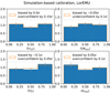 |
Fig. 13. Distributions of |

In the case of the emulator, the  histograms feature small systematic biases, as well as slight under- or overconfidence. These effects are of the order of 0.1σ and consistent with sampling noise. For example, the bottom-left histogram of Fig. 13 are what one would obtain if the true posterior were a N(0, 1) distribution, but the inferred posterior a N(−0.1, 0.952) distribution. The biases observed here are consistent with Table 4, with the difference explainable by a possible mismatch between the median and the mean of the posteriors i.e. their non-Gaussianity.
There again, the NDE and the BNN underperform in comparison, as shown on Figs. 15 and 14. The  histograms display higher bias (up to ∼0.25σ) and in a few cases, under- and overconfidence. Given the histograms of the previous section, the worse performance of the SBI methods in the SBC test are not unexpected. We note that the histograms in the previous sections measure the difference between the true parameters and the position of the maximum of likelihood, while what we interpret as a bias when using the SBC characterises the median of the distribution. Furthermore, we extracted quantitative information (bias and over/underconfidence) from the SBC by comparing our histograms with what we would obtain assuming that the true and recovered posteriors are Gaussian (with different parameters). It is possible that if the recovered posterior differs from the true one by, for example, its skewness or kurtosis, we would interpret this as bias and over/underconfidence. Since the biases measured using the maxima of likelihood are different from the ones measured using SBC (hence, using medians), we expect non-Gaussian posteriors (see the non-Gaussian posterior recovered by the BNN on Fig. 12, and differences in the biases measured on Tables 5, 4 and Fig. 15). Still, it appears that the SBI methods display larger errors and LorEMU leads to consistently better results. Recall that the point of using the SBI networks is to describe the likelihood and posterior with mixture models. The added flexibility may in theory allow the networks to fit the true non-Gaussian target distribution, but it also means they are harder to constrain and require more training samples during training to reach the optimal performance. Moreover, in a regime where thermal noise is the dominant stochastic process, the assumed Gaussian likelihood of LorEMU may be very close to the true likelihood. Finally, the architectures of the SBI networks are more complex than the emulator, and algorithmic improvements remain possible.
Although the setups are different, Prelogović & Mesinger (2023) explore a 5D parameter space with 21cmFAST and train Gaussian Mixture Model NDE to fit the likelihood of their model (with a noise corresponding to 1000 h of SKA integration, while we use 100 h). They notice a massive improvement in performance between training on ∼5700 examples and on ∼28 000 examples. LORELI II contains ‘only’ 10 000 simulations, it is therefore possible that our training sample does not contain enough simulations to benefit from the possibility of fitting the true likelihood/posterior with neutral networks. In other words, in our setup, we obtained better results with a well-evaluated approximate likelihood rather than with a comparatively poorly constrained likelihood or posterior. Still, the errors we observe are of the order of a fraction of the impact of the thermal noise and we can be reasonably confident in the results of our three inference pipelines.
5. Inference on HERA upperlimits
Upper limits on the power spectrum produced by the HERA interferometer and given in Abdurashidova et al. (2022) are close to the most intense signals in the LORELI II database and might therefore constrain our models. All the inferences shown in the previous sections were done not on upper limits but on a clean simulated signal or on a mock detection, i.e. a simulated signal to which a noise realisation was added. In the case of upper limits, the target of inference is assumed to be the 21-cm signal, a noise realisation, and systematics (such as foreground residuals and RFI) affecting the signal. While we model the effect of the thermal noise as a Gaussian random variable, the systematics affect the signal in an unknown, non-trivial way. To take them into account, the authors of Abdurashidova et al. (2022, 2023) assume that they form a function S that adds an unknown amount of power in each (k, z) bin independently and regardless of the signal itself (and therefore of the astrophysical parameters). Hence, the likelihood in Eq. (6) becomes
 (21)
(21)
where P21 is the inference target and y the simulated signal. We are only interested in the posterior on the astrophysical parameters, which suggests marginalising over the systematics S. If we assume a diagonal covariance, which is a rough approximation (it is unlikely that the systematics level in adjacent k bins are uncorrelated), and integrate over S ∈ [0, +∞[, then the log-likelihood takes the form
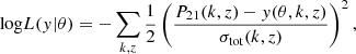
![Mathematical equation: $$ \begin{aligned} {\log }L(y | \theta ) = \sum _{k,z} \frac{1}{2} \left( 1 + \mathrm{{erf}}\left[ \frac{P_{21}(k,z) - y(\theta , k,z )}{ \sqrt{2} \sigma _{\rm tot}(k,z)} \right] \right). \end{aligned} $$](/articles/aa/full_html/2025/06/aa52901-24/aa52901-24-eq43.gif) (22)
(22)
This new form of the explicit likelihood can easily be used with the emulator in an MCMC inference pipeline. The result of an inference done with this method are shown on Fig. 16. Perhaps unsurprisingly, given the levels of the HERA upper limits, the database is not strongly constrained. The 1D posteriors for the escape fraction and the star formation parameters closely resemble the priors, but the upper limits give some constraints on the X-ray related parameters, fX and rH/S. Strikingly, low values of fX, denoting a low level of heating and a strong 21-cm signal (both on average and in its fluctuations) are deemed less likely to describe the HERA data. High values of rH/S, which imply a delayed heating as harder X-rays have a larger mean free path in the neutral IGM, are also slightly constrained, as is evident in the 2D (fX, rH/S) posterior. Hence, these upper limits start to disfavour the ‘cold’ Reionisation scenarios possible in LICORICE. Quantitatively, it must be noted that the 95% confidence contours shown on Fig. 16 are the regions that contain 95% of the integrated probability and are therefore very much prior dependent. While the priors are physically motivated, the design of the database was done under numerical constraint: picking larger priors would cause a sparser sampling of the selected region in parameter space and could impede the training of the networks. Hence, to an extent, the exact cut-offs of the parameters range were arbitrary. Changing them would affect the exact shape of the posterior which must therefore not be over-interpreted. However, our qualitative result that low-heating models are less likely to describe the early Universe is consistent with the conclusions of Abdurashidova et al. (2023).
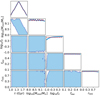 |
Fig. 16. Inference on the latest HERA upper limits using the stacked LorEMU. Priors are shown in red, and the 95% contours of the posteriors in blue. The posteriors over the star formation parameters are identical to the corresponding priors, but in the case of fX, they show a significant departure from the prior. Models with low X-ray intensity (log10fX ≲ −0.6) are deemed less likely to match the observations by HERA. |
We note that this prior-dependency is less of an issue for the results of the mock inferences shown, for example, on Fig. 12 as the astrophysical parameters of the inference targets are near the centre of the parameter space explored in LORELI II and the posteriors smoothly vanish as they approach the edges of the flat prior. Should the signal be detected, the posteriors inferred on such detection could be dangerously close to the edges of the prior. In this case, it would be wise to increase the priors by extending the database.
Nonetheless, Fig. 16 and the equivalent figure obtained using LORELI I in Meriot & Semelin (2024) show the first inferences on actual instrumental data that rely on full 3D hydro-radiative simulations.
6. Conclusions
In this work, we have presented the LORELI II database, a suite of 10 000 moderate-resolution simulations of the EoR that were produced using the latest version of the Licorice hydro-radiative simulation code. This dataset spans a 5D astrophysical parameter space, and star formation parameters, X-ray emissivity and spectra, and UV escape fraction are varied. We used the LORELI II power spectra13 as a training set to explore and compare three machine learning-powered inference methods. The first, already introduced with LORELI I in Meriot & Semelin (2024), consists of training a network to emulate the 21-cm power spectrum of Licorice simulations and using the trained emulator in an MCMC pipeline in order to perform the inference. By averaging the prediction of ten independently trained emulators, we reached ∼3% accurate emulated power spectra and obtained reasonable inference results. However, this method relies on an explicit functional form for the likelihood, which we chose to be Gaussian. As discussed in Prelogović & Mesinger (2023), this Gaussian shape is an approximation. We studied two other methods that rely on SBI in order to relax this approximation and assess whether it allows meaningful improvements. The SBI methods we studied are the use of an NDE to fit the implicit likelihood of the Licorice simulation code and the use of a BNN to directly predict the posterior over the parameters. These methods use parametric functions to fit the desired distributions, and therefore do not assume a fixed approximate shape for the likelihood.
We insist on the fact that the performance of inference methods cannot be measured and compared by studying the inference on a single signal and must be assessed statistically. To this end, we first compared the inference results on 100 random un-noised signals. Since the instrument noise is the dominant source of stochasticity in our setup, we expected the distribution of the difference between the true values of the astrophysical parameters and the maxima of likelihood to be small. According to this simple metric, the NDE shows the most systematic bias while the BNN shows dispersed results, and the emulator performs the best. To provide a more robust analysis, we performed an SBC. We counted how many times the true value of the parameters lie in each quantile of 1D posteriors across many inferences on noised signals. Following Talts et al. (2018), the results should ideally be uniformly distributed. However, for all methods and parameters we observed significant, albeit weak, deviations from uniformity. To make sense of these deviations, we compared them with the deviations we would obtain assuming that the true posteriors are Gaussian and that the inferred posteriors are comparatively biased or over- or underconfident Gaussian. There again, we found that the emulator performs systematically better than the other methods, with errors up to ∼0.15σ while the BNN and NDE exhibit biases and overconfidence up to ∼0.25σ. Still, these systematic errors are of a fraction of a parameter grid interval, which may indicate that we are limited by the density of the training set in parameter space. As in Meriot & Semelin (2024), we applied the emulator to the latest HERA upper limits and obtained weak constraints on fX, which is consistent with Meriot & Semelin (2024) and Abdurashidova et al. (2022).
In conclusion, we are able to perform inferences with our 3D radiative transfer simulation codes, but whether there is in practice a benefit to using SBI instead of the emulator and the approximate likelihood to infer on 100 h SKA data, even with better sampling, remains an open question. Another aspect, is that SBI could show more benefits compared to an emulator if the inference was performed on summary statistics encoding non-Gaussian information, such as the Pixel Distribution Function, some compressed version of the bispectrum, or various flavours of wavelet statistics. This will be the subject of future works.
In any case, it is likely that inference on 1000 h SKA data would require a more refined parameter grid, as the corresponding extent of the 68% contour would be significantly smaller than the current grid step, hindering the training of the networks. Hence, LORELI II might suffice for us to interpret upper limits on the power spectrum, perhaps even a first detection of the signal, but long-term applications will require an upgrade to the database. This is not without hassle. For LORELI II, we stored ∼50 snapshots for each simulation as well as particle light cones, amounting to more than one PB of data. An expanded version of LORELI will require severe pruning of the stored data.
Although improving the training sample can only be beneficial, another question remains. We have measured differences between the results of inference methods applied to the same physical model, but we do not know how they compare to the differences between the results of the same inference methods applied to different physical models.
Different simulation codes are parametrised differently and posteriors on the astrophysical parameters are therefore difficult to compare, but we can make an inference on intermediate quantities present in all codes (e.g. the ionisation fraction, the bubble size distribution, properties of the galaxy population). Zhou & La Plante (2022) provide an example of a prediction of the optical depth τT by neural networks trained on a semi-analytical model but applied to a different model. They obtained arguably poor results, demonstrating that their neural networks imperfectly generalise to data generated using other models. This might not surprise the data scientist, but it is an obstacle for the physicist and the 21-cm community, as it suggests that inference on real data of model-agnostic quantities will give model-dependent results. As high-redshift observations become more common, the non-21-cm related constraints on our models increase, and these models may converge to similar source models, for example. Still, it may well be that the impact of this ‘model uncertainty’ exceeds the difference between inference methods that we presented in this work, and this topic may require a lot of attention from the community in the future. Additionally, the physical modelling in the current version of LICORICE is not without limitations. Possible improvements include the stochasticity in the star formation model (e.g. Poisson fluctuations in the CMF), the sharpness of the ionisation fronts, the modelling of subgrid recombination or including the effect of local gas velocities in the computation of the Wouthuysen-Field coupling (which is absent from the semi-analytical code SPINTER). This work serves as a proof of concept, and interpretations of a future measurement of the 21-cm signal may rely on other 3D hydro-radiative simulation codes.
Square Kilometre Array.
Low-Frequency Array.
New Extension in Nançay Upgrading LOFAR.
Hydrogen Epoch of Reionization Array.
Murchison Widefield Array.
Experiment to Detect the Global EoR Signature.
Smoothed-Particle Hydrodynamics.
Thus neglecting the lightcone effect (Datta et al. 2012). However, we do not expect this effect to significantly alter the signal-to-noise ratio of our spectra nor the dependency of the spectra on the astrophysical parameters, so our conclusions should be insensitive to this effect.
The mock true and infered posteriors were both sampled 10 000 times to reduce the statistical noise.
Available at https://21ssd.obspm.fr/
Acknowledgments
This project was provided with computer and storage resources by GENCI at TGCC thanks to the grants 2022-A0130413759 and 2023-A0150413759 on the supercomputer Joliot Curie’s ROME partition. This work was granted access to the HPC resources of MesoPSL financed by the Region Ile de France and the project Equip@Meso (reference ANR-10-EQPX-29-01) of the programme Investissements d’Avenir supervised by the Agence Nationale pour la Recherche.
References
- Abdurashidova, Z., Aguirre, J. E., Alexander, P., et al. 2022, ApJ, 924, 51 [NASA ADS] [CrossRef] [Google Scholar]
- Abdurashidova, T. H. C. Z., Adams, T., Aguirre, J. E., et al. 2023, ApJ, 945, 124 [NASA ADS] [CrossRef] [Google Scholar]
- Ade, P. A., Aghanim, N., Arnaud, M., et al. 2016, A&A, 594, A13 [NASA ADS] [CrossRef] [EDP Sciences] [Google Scholar]
- Aghanim, N., Akrami, Y., Ashdown, M., et al. 2020, A&A, 641, A6 [NASA ADS] [CrossRef] [EDP Sciences] [Google Scholar]
- Alsing, J., & Wandelt, B. 2018, MNRAS, 476, L60 [NASA ADS] [CrossRef] [Google Scholar]
- Alsing, J., Charnock, T., Feeney, S., & Wandelt, B. 2019, MNRAS, 488, 4440 [Google Scholar]
- Appel, A. W. 1985, SIAM J. Sci. Stat. Comput., 6, 85 [NASA ADS] [CrossRef] [Google Scholar]
- Atek, H., Richard, J., Kneib, J. P., & Schaerer, D. 2018, MNRAS, 479, 5184 [Google Scholar]
- Barnes, J., & Hut, P. 1986, Nature, 324, 446 [NASA ADS] [CrossRef] [Google Scholar]
- Bouwens, R. J., Aravena, M., Decarli, R., et al. 2016, ApJ, 833, 72 [NASA ADS] [CrossRef] [Google Scholar]
- Bouwens, R. J., Oesch, P. A., Stefanon, M., et al. 2021, AJ, 162, 47 [NASA ADS] [CrossRef] [Google Scholar]
- Bouwens, R., Illingworth, G., Oesch, P., et al. 2023, MNRAS, 523, 1009 [NASA ADS] [CrossRef] [Google Scholar]
- Bowman, J. D., Rogers, A. E., Monsalve, R. A., Mozdzen, T. J., & Mahesh, N. 2018, Nature, 555, 67 [NASA ADS] [CrossRef] [Google Scholar]
- Breitman, D., Mesinger, A., Murray, S. G., et al. 2024, MNRAS, 527, 9833 [Google Scholar]
- Bye, C. H., Portillo, S. K. N., & Fialkov, A. 2022, ApJ, 930, 79 [NASA ADS] [CrossRef] [Google Scholar]
- Chapman, E., & Jelić, V. 2019, The Cosmic 21-cm Revolution, 6–1 [Google Scholar]
- Ciardi, B., Stoehr, F., & White, S. D. 2003, MNRAS, 343, 1101 [NASA ADS] [CrossRef] [Google Scholar]
- Cook, S. R., Gelman, A., & Rubin, D. B. 2006, J. Comput. Graphical Stat., 15, 675 [Google Scholar]
- Datta, K. K., Mellema, G., Mao, Y., et al. 2012, MNRAS, 424, 1877 [NASA ADS] [CrossRef] [Google Scholar]
- Doussot, A., & Semelin, B. 2022, A&A, 667, A118 [NASA ADS] [CrossRef] [EDP Sciences] [Google Scholar]
- Field, G. B. 1958, Proc. IRE, 46, 240 [NASA ADS] [CrossRef] [Google Scholar]
- Finkelstein, S. L., Ryan, R. E., Papovich, C., et al. 2015, ApJ, 810, 71 [NASA ADS] [CrossRef] [Google Scholar]
- Furlanetto, S. R., & Pritehard, J. R. 2006, MNRAS, 372, 1093 [NASA ADS] [CrossRef] [Google Scholar]
- Furlanetto, S. R., Peng Oh, S., & Briggs, F. H. 2006, Phys. Rep., 433, 181 [NASA ADS] [CrossRef] [Google Scholar]
- Gal, Y., & Ghahramani, Z. 2016, 33rd Int. Conf. Mach. Learn., ICML 2016, 3, 1651 [Google Scholar]
- Ghara, R., Mellema, G., Giri, S. K., et al. 2018, MNRAS, 476, 1741 [NASA ADS] [CrossRef] [Google Scholar]
- Greig, B., & Mesinger, A. 2015, MNRAS, 449, 4246 [NASA ADS] [CrossRef] [Google Scholar]
- Greig, B., & Mesinger, A. 2018, MNRAS, 477, 3217 [NASA ADS] [CrossRef] [Google Scholar]
- Hortúa, H. J., Volpi, R., & Malagò, L. 2020, Parameters Estimation From the 21 cm Signal Using Variational Inference, Tech. rep., https://doi.org/10.48550/arXiv.2005.02299 [Google Scholar]
- Ishigaki, M., Kawamata, R., Ouchi, M., et al. 2018, ApJ, 854, 73 [NASA ADS] [CrossRef] [Google Scholar]
- Jennings, W. D., Watkinson, C. A., Abdalla, F. B., & McEwen, J. D. 2019, MNRAS, 483, 2907 [NASA ADS] [CrossRef] [Google Scholar]
- Jospin, L. V., Laga, H., Boussaid, F., Buntine, W., & Bennamoun, M. 2022, IEEE Comput. Intell. Mag., 17, 29 [Google Scholar]
- Lewis, J. S., Ocvirk, P., Sorce, J. G., et al. 2022, MNRAS, 516, 3389 [NASA ADS] [CrossRef] [Google Scholar]
- McLeod, D. J., McLure, R. J., & Dunlop, J. S. 2016, MNRAS, 459, 3812 [NASA ADS] [CrossRef] [Google Scholar]
- McQuinn, M., Zahn, O., Zaldarriaga, M., Hernquist, L., & Furlanetto, S. R. 2006, ApJ, 653, 815 [NASA ADS] [CrossRef] [Google Scholar]
- Mellema, G., Iliev, I. T., Alvarez, M. A., & Shapiro, P. R. 2006, New Astron., 11, 374 [NASA ADS] [CrossRef] [Google Scholar]
- Meriot, R., & Semelin, B. 2024, A&A, 683, A24 [NASA ADS] [CrossRef] [EDP Sciences] [Google Scholar]
- Mertens, F. G., Mevius, M., Koopmans, L. V., et al. 2020, MNRAS, 493, 1662 [NASA ADS] [CrossRef] [Google Scholar]
- Mineo, S., Gilfanov, M., & Sunyaev, R. 2011, Astron. Nachr., 332, 349 [Google Scholar]
- Munshi, S., Mertens, F. G., Koopmans, L. V., et al. 2024, A&A, 681, A62 [NASA ADS] [CrossRef] [EDP Sciences] [Google Scholar]
- Ocvirk, P., Aubert, D., Sorce, J. G., et al. 2020, MNRAS, 496, 4087 [NASA ADS] [CrossRef] [Google Scholar]
- Oesch, P. A., Bouwens, R. J., Illingworth, G. D., Labbé, I., & Stefanon, M. 2018, ApJ, 855, 105 [Google Scholar]
- Papadopoulou, O., Zampoglou, M., Papadopoulos, S., & Kompatsiaris, I. 2016, Thesis, 43, 72 [Google Scholar]
- Papamakarios, G., & Murray, I. 2016, Adv. Neural Inf. Process.Syst., 29, 1036 [Google Scholar]
- Prelogović, D., & Mesinger, A. 2023, MNRAS, 524, 4239 [CrossRef] [Google Scholar]
- Prelogović, D., & Mesinger, A. 2024, A&A, 688, A199 [NASA ADS] [CrossRef] [EDP Sciences] [Google Scholar]
- Pritchard, J. R., & Loeb, A. 2012, Rep. Prog. Phys., 75, 086901 [NASA ADS] [CrossRef] [Google Scholar]
- Reis, I., Fialkov, A., & Barkana, R. 2021, MNRAS, 506, 5479 [NASA ADS] [CrossRef] [Google Scholar]
- Rubiño-Martín, J. A., Betancort-Rijo, J., & Patiri, S. G. 2008, MNRAS, 386, 2181 [CrossRef] [Google Scholar]
- Saxena, A., Cole, A., Gazagnes, S., et al. 2023, MNRAS, 525, 6097 [NASA ADS] [CrossRef] [Google Scholar]
- Schaeffer, T., Giri, S. K., & Schneider, A. 2023, MNRAS, 526, 2942 [NASA ADS] [CrossRef] [Google Scholar]
- Semelin, B., Eames, E., Bolgar, F., & Caillat, M. 2017, MNRAS, 472, 4508 [NASA ADS] [CrossRef] [Google Scholar]
- Semelin, B., Mériot, R., Mertens, F., et al. 2023, A&A, 672, A162 [NASA ADS] [CrossRef] [EDP Sciences] [Google Scholar]
- Sheth, R. K., & Tormen, G. 2002, MNRAS, 329, 61 [Google Scholar]
- Singh, S., Nambissan T., J., Subrahmanyan, R., et al. 2022, Nat. Astron., 6, 607 [NASA ADS] [CrossRef] [Google Scholar]
- Sobacchi, E., & Mesinger, A. 2014, MNRAS, 440, 1662 [NASA ADS] [CrossRef] [Google Scholar]
- Springel, V. 2005, MNRAS, 364, 1105 [Google Scholar]
- Talts, S., Betancourt, M., Simpson, D., Vehtari, A., & Gelman, A. 2018, ArXiv e-prints [arXiv:1804.06788] [Google Scholar]
- Wouthuysen, S. A. 1952, Physica, 18, 75 [NASA ADS] [CrossRef] [Google Scholar]
- Yoshiura, S., Pindor, B., Line, J. L., et al. 2021, MNRAS, 505, 4775 [CrossRef] [Google Scholar]
- Zhao, X., Mao, Y., Cheng, C., & Wandelt, B. D. 2022a, ApJ, 926, 151 [NASA ADS] [CrossRef] [Google Scholar]
- Zhao, X., Mao, Y., & Wandelt, B. D. 2022b, ApJ, 933, 236 [NASA ADS] [CrossRef] [Google Scholar]
- Zhou, Y., & La Plante, P. 2022, PASP, 134, 044001 [Google Scholar]
All Tables
Relative bias (i.e. ratio of error and standard deviation of the posterior) for all methods and parameters.
Absolute bias (i.e. ratio of error and grid step) for all methods and parameters.
All Figures
|
Fig. 1. Thomson scattering optical depth of the LORELI II simulations. Measurements by Planck 2015 and 2018 are also reported (Aghanim et al. 2020; Ade et al. 2016). The LORELI simulations are within 3σ of these constraints, although they were not used to calibrate the database per se. |
| In the text | |
|
Fig. 2. UV luminosity functions of the LORELI II simulations at z ∼ 6, 8, 10. The dark green region shows, for each magnitude bin, where the middle 50% of the simulations lie, while the light green region shows where all simulations lie. We compare the simulated results with observations from Finkelstein et al. (2015), Oesch et al. (2018), Ishigaki et al. (2018), Atek et al. (2018), Bouwens et al. (2021, 2023). |
| In the text | |
|
Fig. 3. Average global δTb of the 10 000 LORELI II simulations, colour-coded according to the X-ray intensity parameter fX. |
| In the text | |
|
Fig. 4. Top: Randomly selected emulated power spectra. Bottom: Corresponding spectra from LORELI II. This figure is a simple illustration of the performances of LorEMU. |
| In the text | |
|
Fig. 5. Performance metrics of an instance of LorEMU, averaged over the test set. The network performs better where the CV and thermal noise are weak (see text for details). |
| In the text | |
|
Fig. 6. Similar to 5 but for the average predictions of ten independently trained instances of LorEMU, leading to a significant performance improvement. For instance, the relative error typically decreases by a factor three. |
| In the text | |
|
Fig. 7. Results of inference on a noiseless LORELI II power spectrum using ten independently trained versions of the LorEMU II emulator (red). The emulators show a non-negligible variance. This uncertainty can be mitigated by averaging the predictions of the different instances of LorEMU during the inference (black). On 2D posteriors, only the 1σ contours are shown, for clarity. |
| In the text | |
|
Fig. 8. Left: Mean standard deviation of the predicted distributions of each parameter by the BNN. For a single example, the mean was obtained by averaging the predicted means over 100 forward-passes (shown as solid lines), and the vertical width of the shaded regions show the dispersion of the results across the validation set. This quantifies the aleatoric uncertainty (i.e. the uncertainty caused by the noise in the data). Right: Standard deviation of the predicted means. This is the epistemic uncertainty (i.e. the error caused by the sparsity of the training sample). It is an order of magnitude smaller than the aleatoric uncertainty, indicating that the instrumental noise is the dominant source of variance. |
| In the text | |
|
Fig. 9. Error of the BNN predictions. For each parameter, the shaded regions is centred on the difference between the average predicted mean and the true value, and the vertical width is given by the average standard deviation of the predicted distributions. While the predicted means are very stable (as shown on the right panel of Figure 8), the network shows a significant bias for all parameters save for fX in ∼10% of the cases. |
| In the text | |
|
Fig. 10. Posteriors estimated by repeatedly forward passing a noiseless LICORICE power spectrum to ten independently trained BNNs (green) and to the stacked BNN (black). The results show little variance and seem to converge to slightly biased results. The posterior on rH/S shows a long tail not retrieved by the other inference methods. |
| In the text | |
|
Fig. 11. Similar to 7 but for ten independently trained NDEs. They exhibit a similar amount of training variance as the emulators, but seem to display a larger systematic bias. |
| In the text | |
|
Fig. 12. Inference with all (stacked) networks. All three results agree to a large extent. The maxima of likelihood are close; they are all within 1σ of each other and within a grid step. Nonetheless, the BNN is systematically less confident than the others, while the predictions of NDE are slightly more biased. For clarity, we exclude fesc from the analysis, as it is systematically poorly reconstructed by all three methods. |
| In the text | |
|
Fig. 13. Distributions of |
| In the text | |
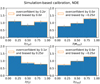 |
Fig. 14. Same as 13 but with the stacked NDE. |
| In the text | |
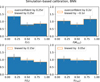 |
Fig. 15. Same as 13 but with the stacked BNN. |
| In the text | |
|
Fig. 16. Inference on the latest HERA upper limits using the stacked LorEMU. Priors are shown in red, and the 95% contours of the posteriors in blue. The posteriors over the star formation parameters are identical to the corresponding priors, but in the case of fX, they show a significant departure from the prior. Models with low X-ray intensity (log10fX ≲ −0.6) are deemed less likely to match the observations by HERA. |
| In the text | |
Current usage metrics show cumulative count of Article Views (full-text article views including HTML views, PDF and ePub downloads, according to the available data) and Abstracts Views on Vision4Press platform.
Data correspond to usage on the plateform after 2015. The current usage metrics is available 48-96 hours after online publication and is updated daily on week days.
Initial download of the metrics may take a while.