© The Authors 2025

1. Introduction

The cosmological 21 cm signal from neutral hydrogen promises to revolutionize astrophysics and cosmology by mapping out the first half of our observable Universe. Experimental efforts to detect this signal fall into two categories. Interferometers such as the Square Kilometre Array (SKA; e.g., Mellema 2013), Hydrogen Epoch of Reionization Array (HERA; Abdurashidova et al. 2022), Low Frequency Array (LOFAR; van Haarlem et al. 2013), and Murchison Widefield Array (MWA; Tingay et al. 2013) are dedicated to measuring the spatial fluctuations of the 21 cm brightness temperature T₂₁. Alternatively, global experiments including the Experiment to Detect the Global Epoch of Reionization Signature (EDGES; Bowman et al. 2018a), Shaped Antenna measurement of the background RAdio Spectrum (SARAS; Singh et al. 2018; Bevins et al. 2022), Radio Experiment for the Analysis of Cosmic Hydrogen (REACH; de Lera Acedo et al. 2022), Mapper of the IGM Spin Temperature (MIST; Monsalve et al. 2024), and Large Aperture Experiment to Detect the Dark Ages (LEDA; Greenhill & Bernardi 2012) aim to detect the spatially averaged (global) 21 cm signal ${\overline{T}}_{21}$.

The first detection of the cosmic 21 cm signal was claimed by the EDGES experiment in 2018 (Bowman et al. 2018a, hereafter B18), which measured a flattened ${\overline{T}}_{21}$ absorption profile centered around z ∼ 17 with an amplitude of ${500}_{-200}^{+500}$ mK (at 99% credible interval). A subsequent Bayesian reanalysis of the entire signal chain by Murray et al. (2022) confirmed the presence of such a signal in the data. This signal is about twice as deep as the maximum amplitude allowed by standard models in which baryons cool at most adiabatically and the radio background is dominated by the cosmic microwave background (CMB). As has been pointed out in many previous studies, a cosmological origin for the EDGES signal requires one of two broad mechanisms: (i) extra gas cooling, such as interactions between dark matter (DM) and baryons (Barkana 2018; Muñoz & Loeb 2018; Berlin et al. 2018), and early gas-CMB decoupling in early dark energy models (Hill & Baxter 2018); or (ii) an excess radio background component in addition to the CMB (Feng & Holder 2018; Ewall-Wice et al. 2018, 2020; Mirocha & Furlanetto 2019; Reis et al. 2020).

It is very challenging to perform accurate inference from the global 21 cm signal. Astrophysical and terrestrial foregrounds are four to six orders of magnitude brighter than the cosmological signal (e.g., Pritchard & Loeb 2012; Hibbard et al. 2023), and unlike interferometers, global 21 cm experiments cannot clean the signal by comparing different pointings and sightlines (e.g., Nasirudin et al. 2020). In addition to astrophysical foregrounds, other systematics such as the Earth’s ionosphere (e.g., Datta et al. 2016; Shen et al. 2021), antenna beam effects (e.g., Mahesh et al. 2021; Sims et al. 2023), and signal-chain defects (e.g., Monsalve et al. 2017; Murray et al. 2022) can further obscure the signal and potentially lead to false reconstructions (Tauscher et al. 2020; Hibbard et al. 2023). Therefore, the interpretation of the EDGES results requires detailed characterization of these contaminants together with the cosmic signal, with all of the resulting parameters being constrained through Bayesian inference.

The 21 cm signal reported in B18 was obtained by fitting the EDGES sky temperature data with a flat-Gaussian ${\overline{T}}_{21}$ profile and a five-term polynomial foreground model. Subsequent analysis in Hills et al. (2018) and Singh & Subrahmanyan (2019) showed that the best-fit profile found in B18 requires an un-physical foreground and that the EDGES data can also be fit with multiple ${\overline{T}}_{21}$ shapes that are different from those used in B18. Sims & Pober (2020) (hereafter SP20) extended these analyses by considering a set of models with various combinations of the cosmic signal, residual calibration systematics, and foregrounds. After comparing the Bayesian evidence for a total of 128 models, SP20 found that the models that are not strongly disfavored include a flattened Gaussian cosmic signal with a non-standard depth and sinusoidal calibration residuals. Subsequent data from the SARAS3 experiment disfavored the presence of an EDGES-like cosmic signal (Singh et al. 2022).

It is somewhat surprising that many analyses have reached different conclusions about the existence and (or) depth of the cosmic 21 cm profile in EDGES data. Ideally, any interpretation should use self-consistent forward models with physically informed priors. The vast majority of radio excess and gas cooling analysis (see e.g., Ewall-Wice et al. 2018, 2020; Barkana 2018; Muñoz & Loeb 2018; Mirocha & Furlanetto 2019; Reis et al. 2020; Mebane et al. 2020) instead compute a “pseudo likelihood” using only a summary of the data, typically the center and (or) width of the B18 profile. This approach is intrinsically problematic since the B18 profile was computed assuming a phenomenological “flattened Gaussian” ${\overline{T}}_{21}$ and therefore cannot be interpreted directly with a different (e.g., physical) model for the ${\overline{T}}_{21}$¹.

Here we directly forward-model the EDGES sky temperature data, comparing the Bayesian evidence for a range of foreground models and residual calibration systematics. Unlike the analytic and phenomenological models used in B18, SP20, and Murray et al. (2022), we build on the cosmological 21cmFAST simulation code (e.g., Mesinger et al. 2011; Murray et al. 2020), including an inhomogeneous excess radio background sourced from the first molecular-cooling galaxies hosted by ∼10⁵ − 10⁸ M_⊙ halos. These primordial galaxies are expected to be dominated by metal-free population III (Pop III) stars and their remnants, which could have very different properties compared to later generations (e.g., Woosley et al. 2002; Heger et al. 2003). For simplicity, we refer to molecular-cooling galaxies as “Pop III galaxies” in this work. Later generations of galaxies form out of Pop III galaxy seeds and mainly reside in more massive dark matter halos (> 10⁸ M_⊙), for which atomic cooling is efficient. Analogously to Pop III galaxies, here we refer to atomic cooling galaxies as Pop II galaxies, as most of their stellar population is formed out of pre-enriched gas (e.g., Bromm & Larson 2004; Trenti 2010; Salvaterra et al. 2011).

Previously it was shown in Mirocha & Furlanetto (2019) and Reis et al. (2020) that in order for Pop II galaxies to reproduce the amplitude of the B18 feature, the corresponding radio background should exceed present-day measurements from the Absolute Radiometer for Cosmology, Astrophysics, and Diffuse Emission 2 (ARCADE2; Fixsen et al. 2011) by orders of magnitude. This tension was resolved in an ad-hoc manner by introducing a phenomenological redshift cutoff parameter, z_off (see e.g., Mirocha & Furlanetto 2019; Reis et al. 2020; Sikder et al. 2024a,b), below which galactic radio emission is quenched. In contrast, Pop III galaxies are susceptible to feedback from the Lyman Werner (LW) background (e.g., Qin et al. 2020a; Muñoz et al. 2022), which eventually sterilizes star formation inside them. As a result, the radio emission from Pop III galaxies decays naturally once an LW background is established, thus making Pop III galaxies a natural candidate to explain EDGES while being consistent with ARCADE2 measurements. Indeed, Mebane et al. (2020) studied the radio background that could be provided by Pop III galaxies, motivated by B18; however, they did not jointly model foreground and instrumental systematics.

In this work, we determine whether the EDGES data prefer such a physical model for a high-redshift radio-background excess. We forward-model the global signal, varying Pop III galaxy properties, foregrounds, and experimental calibration residuals. We vary the complexity of the foreground and calibration models, comparing their Bayesian evidence. We include complementary data from ARCADE2 and Planck. To speed up the inference, we trained an emulator of summary observables in our model, and we provide it as a new option in the public 21cmEMU² package (Breitman et al. 2024).

The paper is organized as follows. Sect. 2 reviews the EDGES observation, while Sect. 3 details our model for Pop III radio galaxies. We build some physical intuition about our model with an illustrative example in Sect. 4 and then discuss our model for foreground emission and systematics in Sect. 5. Our likelihoods and inference methodology are detailed in Secs. 6 and 7, respectively. We show results for fitting a B18-based pseudo-likelihood in Sect. 8 before presenting results for self-consistent inferences in Sect. 9. Finally we present discussions and caveats in Sect. 10 and conclude in Sect. 11. We assume a Λ_CDM cosmology with the relevant parameters set by Planck 2018 results (Planck Collaboration VI 2020): H₀ = 67.66 km s⁻¹ Mpc⁻¹, Ω_Λ = 0.6903, Ω_m = 0.3096, Ω_c = 0.2607, Ω_b = 0.0489, ln(10¹⁰A_s) = 3.047, and n_s = 0.967.

2. EDGES observations

We used the same publicly available EDGES data as in B18 (see Murray et al. 2022), namely the sky temperature spectrum T_sky³. This section gives a brief review of the observation and data processing (for more details, see B18).

The data are from the EDGES low-band instruments operating over 50–100 MHz frequencies, which correspond to 13 ≤ z ≤ 27. The data were collected between 2016 and 2017 and consist of a total of 138 days of observation, after the initial quality cuts (Murray et al. 2022). The raw data are contaminated by transient sources such as the sun, weather and radio frequency interference (Tauscher et al. 2020), the calibration and data-analysis pipeline removes and corrects for these effects resulting in T_sky, which was assumed to consist of the beam-weighted foregrounds (FGs) and the global cosmic 21 cm signal (Tauscher et al. 2020):

$$\begin{array}{c}\hfill T_{=}{T}_{+}{\overline{T}}_{21}.\end{array}$$(1)

B18 modeled the FGs as a five-term log-polynomial, motivated by the known properties of the Galactic synchrotron spectrum and the Earth’s ionosphere,

$$\begin{array}{cc}\hfill T_{\mathrm{FG}}& \approx a_0{\left(\frac{\nu }{{\nu }_{\mathrm{c}}}\right)}^{-2.5}+a_1{\left(\frac{\nu }{{\nu }_{\mathrm{c}}}\right)}^{-2.5}ln\left(\frac{\nu }{{\nu }_{\mathrm{c}}}\right)\hfill \\ \hfill & +a_2{\left(\frac{\nu }{{\nu }_{\mathrm{c}}}\right)}^{-2.5}{[ln\left(\frac{\nu }{{\nu }_{\mathrm{c}}}\right)]}^2+a_3{\left(\frac{\nu }{{\nu }_{\mathrm{c}}}\right)}^{-4.5}+a_4{\left(\frac{\nu }{{\nu }_{\mathrm{c}}}\right)}^{-2}.\hfill \end{array}$$(2)

Here ν is the observing frequency, a_n are fitting coefficients, and v_c = 75 MHz is the central frequency of the observing band.

The cosmic 21 cm signal in Eq. (1) was modelled as a flattened-Gaussian:

$$\begin{array}{c}\hfill {\overline{T}}_{21}=-A\left[\frac{1-exp(-{\tau }^B)}{1-exp(-\tau )}\right],\end{array}$$(3)

with

$$\begin{array}{c}\hfill B=\frac{4{(\nu -{\nu }_0)}^2}{w^2}ln[-\frac{1}{\tau }ln\left(\frac{1{+}^{-\tau }}{2}\right)],\end{array}$$(4)

where A, ν₀, w and τ are model parameters representing the depth, central frequency, full-width at half-maximum and flatness of the signal, respectively. Inference using this model resulted in a noise-like residual with an RMS (root mean square) of 25 mK, and constrained the ${\overline{T}}_{21}$ parameters to $A=0.5_{-0.2}^{+0.5}\mathrm{K}$, ν₀ = 78 ± MHz, $w={19}_{-3}^{+4}\mathit{MHz}$ and $\tau =7_{-3}^{+3}$, where the bounds represents 99% credible intervals (C.I.s).

In this work, we forward-model the calibrated brightness temperature data, T_sky, using our own physical model for the 21 cm signal, ${\overline{T}}_{21}$, as well as different basis sets for FGs, T_FG, and possible calibration residuals, T_cal (see Equation (37)). We describe our models for each in turn below.

3. Enhanced 21 cm absorption via radio-loud, molecular-cooling galaxies

We extend the public 21cmFAST code (Mesinger et al. 2011); Murray:2020trn to include an inhomogeneous radio background from galaxies. Starting from cosmological initial conditions, 21cmFAST simulates 3D lightcones of density, star formation and various radiation fields to be used for computing the thermal and ionization evolution of the inter-galactic medium (IGM). Here we summarize some of the salient points of this procedure, highlighting the novelties of our model; readers are encouraged to consult the above references for more details on the 21cmFAST code.

We make the ansatz that the very first molecularly cooled Pop III galaxies were responsible for the radio excess putatively observed by EDGES. The star formation in Pop III galaxies is transient as they are sterilized by the build-up of a LW background and feedback from photoheating (Qin et al. 2020a; Muñoz et al. 2022). Therefore they provide a physical way to establish an early radio background, without having to introduce a “turn-off” redshift (see e.g., Mirocha & Furlanetto 2019; Reis et al. 2020) so as not to overproduce the present-day radio background. Below we discuss our star formation prescription, and how we model the associated radiation backgrounds using semi-empirical relations.

3.1. Star formation

We assume that stars form in both atomic and molecular cooling halos, and that these can have different properties. Made from the pristine unpolluted metal-free gas, the first (Pop III) stars are expected to form in small molecular-cooling galaxies at z ∼ 20 − 30 (Qin et al. 2020a, 2021; Muñoz et al. 2022), whereas the second (Pop II) generation of stars form from the gas polluted by metallic remnants of Pop III stars and reside in galaxies that accrete gas through atomic-cooling. Their comoving star formation rate density (SFRD) is linked to the halo mass function according to

$$\begin{array}{c}\hfill {}_{=}{\displaystyle \int \mathrm{d}}{M}_{}{\dot{M}}_{\star ,\mathrm{s}}{f}_{\mathrm{duty},\mathrm{s}}\frac{\mathrm{d}n}{\mathrm{d}{M}_{\mathrm{h}}}\left(M_{\mathrm{h}},z|R,{\delta }_{\mathrm{R}}\right).\end{array}$$(5)

Hereafter we use the subscript s to denote Pop II (s = II) and Pop III (s = III) galaxies, M_h is halo mass, and dn/dM_h(M_h,z|Rδ_R is the conditional halo mass function, which gives the differential halo number density for a region of scale R and corresponding overdensity δR. Equation (5) is evaluated in different patches of the simulation box, with the density field modulating (i.e., conditioning; Lacey & Cole 1993; Somerville & Kolatt 1999; Cooray & Sheth 2002) the halo mass function and thus sourcing spatial variations in the SFRD.

The stellar mass of a galaxy is assumed to build up over some fraction, η, of the Hubble time, H⁻¹(z), where H(z) is the Hubble parameter. Thus the star formation rate Ṁ_⋆,s is related to the stellar mass M_⋆,s via

$$\begin{array}{c}\hfill {\dot{M}}_{\star ,}=M_{\star ,}H(z)/\eta ,\end{array}$$(6)

where η is a free parameter between zero and unity, and

$$\begin{array}{c}\hfill M_{\star ,}=f_{\star ,}\left(\frac{{\mathrm{\Omega }}_{\mathrm{b}}}{{\mathrm{\Omega }}_{\mathrm{m}}}\right)M_{.}\end{array}$$(7)

Here f_⋆,s is the fraction of baryons converted into stars,

$$\begin{array}{cc}\hfill f_{\star ,\mathrm{II}}& =min[f_{\star ,10}{\left(\frac{M_{\mathrm{h}}}{{10}^{10}{M}_{\odot }}\right)}^{{\alpha }_{\star ,\mathrm{II}}},1],\hfill \end{array}$$(8)

$$\begin{array}{cc}\hfill f_{\star ,\mathrm{III}}& =min[f_{\star ,7}{\left(\frac{M_{\mathrm{h}}}{{10}^7{M}_{\odot }}\right)}^{{\alpha }_{\star ,\mathrm{III}}},1].\hfill \end{array}$$(9)

Finally in Eq. (5), the duty cycle f_duty, s describes the star formation efficiency inside the halo,

$$\begin{array}{cc}\hfill f_{\mathrm{duty},\mathrm{II}}& =exp(-M_{\mathrm{turn},\mathrm{II}}/M_{\mathrm{h}}),\hfill \end{array}$$(10)

$$\begin{array}{cc}\hfill f_{\mathrm{duty},\mathrm{III}}& =exp(-M_{\mathrm{turn},\mathrm{III}}/M_{\mathrm{h}})exp(-M_{\mathrm{h}}/M_{\mathrm{atom}}).\hfill \end{array}$$(11)

Here the turnover mass M_turn,s characterizes the mass scale below which star formation is strongly suppressed. M_turn,s is determined by various feedback mechanisms and can be expressed as

$$\begin{array}{cc}\hfill M_{\mathrm{turn},\mathrm{II}}& =max(M_{\mathrm{crit}}^{\mathrm{ion}},M_{\mathrm{atom}}),\hfill \end{array}$$(12)

$$\begin{array}{cc}\hfill M_{\mathrm{turn},\mathrm{III}}& =max(M_{\mathrm{crit}}^{\mathrm{ion}},M_{\mathrm{mol}}),\hfill \end{array}$$(13)

where $M_{\mathrm{crit}}^{\mathrm{ion}}$ and M_atom describe photoheating feedback and the atomic cooling threshold (corresponding to a halo virial temperature of 10⁴ K; see Sobacchi & Mesinger 2013; Qin et al. 2020a, 2021).

Efficient star formation inside Pop III galaxies also depends on the inhomogeneous LW background and the local DM-baryon relative velocity. Following Muñoz et al. (2022), we take

$$\begin{array}{c}\hfill M_{\mathrm{mol}}=M_0(z)f_{v_{\mathrm{cb}}}{f}_{\mathrm{LW}},\end{array}$$(14)

where f_vcb is determined by an empirical fit to hydrodymanical simulations (Kulkarni et al. 2021; Schauer et al. 2021), and M₀(z) = 3.3 × 10⁷(1 + z)^−3/2 M_⊙. f_LW describes LW feedback, which is detailed in the next subsection.

3.2. Inhomogeneous cosmic radiation fields

We briefly summarize how we compute the LW, X-ray, ionizing ultraviolet (UV) and radio radiation fields, which are relevant for the 21 cm signal as well as for photo-heating (ionizing) and photo-dissociating (LW) feedback on star formation. We encourage interested readers to see Muñoz et al. (2022) and Qin et al. (2020a) for more details.

3.2.1. Lyman Werner radiation

Lyman Werner radiation (whose photons have energies in the range 11.2–13.6 eV) can photodissociate H₂ molecules through the Solomon process. Pop III galaxies exposed to a high LW flux will therefore have difficulty accreting gas through the H₂ cooling channel, which eventually sterilizes their star formation (e.g., Tegmark et al. 1997; Bromm & Larson 2004). It was shown in Machacek et al. (2001) that the minimum mass of star forming halos, approximated here by the turnover mass M_turn,III in Eq. (13), has a power-law dependency on LW intensity. Motivated by results from hydrodynamic simulations (Kulkarni et al. 2021; Schauer et al. 2021), 21cmFAST adopts the analytic form in Visbal et al. (2014) to parameterize the suppression factor f_LW in Eq. (14),

$$\begin{array}{c}\hfill f_{\mathrm{LW}}=1+A_{\mathrm{LW}}{J}_{\mathrm{LW}}^{{\beta }_{\mathrm{LW}}},\end{array}$$(15)

where A_LW and β_LW are free model parameters, and J_LW is the LW intensity in 10⁻²¹ erg s⁻¹ cm⁻² Hz⁻¹ s⁻¹ at a redshift z and cell position x,

$$\begin{array}{c}\hfill J_{\mathrm{LW}}(z,\mathbf{x})=\frac{c{(1+z)}^3}{4\pi }{\displaystyle {\int }_z^{\infty }}\frac{\mathrm{d}z\prime }{(1+z\prime )H}{ϵ}_{\mathrm{LW}}^{-{\tau }_{\mathrm{LW}}}.\end{array}$$(16)

Here the optical depth τ_LW accounts for resonance attenuation, and ϵ_LW is the LW emissivity from both Pop II and Pop III galaxies (Qin et al. 2020a).

3.2.2. X-ray emission

X-rays that ionize and heat the IGM are primarily emitted by high mass X-ray binaries (HMXBs), which are relatively short-lived and so trace the star formation rate of the host galaxy (e.g., Fragos et al. 2013). Therefore the rest-frame, specific X-ray emissivity ϵ_x is taken to be proportional to the SFRD (consistent with observations of low-redshift star forming galaxies; e.g., Lehmer et al. 2021):

$$\begin{array}{c}\hfill {ϵ}_{(}z,\mathbf{x},\nu )=L_{/}{\times }_{.}\end{array}$$(17)

Here L_x,s/SFR is the specific X-ray luminosity per star formation rate (SFR), which is assumed to follow a power-law frequency spectrum,

$$\begin{array}{c}\hfill L_{/}\propto {\nu }^{{\alpha }_{\mathrm{x}}},\end{array}$$(18)

and α_x is the power-law index. We define the normalization parameter of L_x,s/SFR as

$$\begin{array}{c}\hfill L_{\mathrm{X},\mathrm{III}<2\mathrm{keV}}\equiv {\displaystyle {\int }_{E_0}^{2\mathrm{keV}}}\mathrm{d}E{L}_{/}\mathrm{SFR},\end{array}$$(19)

where E₀ is the energy threshold below which photons are absorbed by the host galaxy (e.g., Das et al. 2017).

3.2.3. Ionizing UV

Reionization of the IGM is assumed to be driven by ionizing UV radiation from massive stars. Following the excursion-set formalism of Furlanetto et al. (2004), 21cmFAST identifies a simulation cell as ionized if the cumulative number of ionizing photons per baryon ${\overline{n}}_{\mathrm{ion}}$ satisfies the following condition over a spherical region with any given radius R,

$$\begin{array}{c}\hfill {\overline{n}}_{\mathrm{ion}}\ge (1+{\overline{n}}_{\mathrm{rec}})(1-{\overline{x}}_{\mathrm{e}}),\end{array}$$(20)

where ${\overline{n}}_{\text{rec}}$ is the cumulative number of recombinations per baryon (see Sobacchi & Mesinger 2014; Qin et al. 2020a), ${\overline{x}}_{\mathrm{e}}$ is the average ionization fraction induced by X-rays, and ${\overline{n}}_{\mathrm{ion}}$ is calculated by

$$\begin{array}{c}\hfill {\overline{n}}_{\mathrm{ion}}=\frac{1}{{\rho }_{\mathrm{b}}}{\displaystyle \sum _{\mathrm{s}}}{\displaystyle \int \mathrm{d}}{M}_{\mathrm{h}}{\varphi }_{\mathrm{s}}{M}_{\star ,\mathrm{s}}{n}_{\gamma ,\mathrm{s}}{f}_{\mathrm{esc},\mathrm{s}},\end{array}$$(21)

where ρ_b is the averaged baryon density within a spherical region of radius R, ϕ_s = f_duty,sdn/dM_h, the stellar mass M_⋆, s is given in Eq. (7), n_γ,s is the number of ionizing photons emitted per stellar baryon, for which we adopt 5 × 10³ for Pop II and 5 × 10⁴ for Pop III. Finally f_esc, s is the fraction of ionizing UV photons that escape the host galaxies normalized at the same characteristic halo mass values as the SFR efficiency:

$$\begin{array}{cc}\hfill f_{\mathrm{esc},\mathrm{II}}& =min[f_{\mathrm{esc},10}{\left(\frac{M_{\mathrm{h}}}{{10}^{10}{M}_{\odot }}\right)}^{{\alpha }_{\mathrm{esc},\mathrm{II}}},1],\hfill \end{array}$$(22)

$$\begin{array}{cc}\hfill f_{\mathrm{esc},\mathrm{III}}& =min[f_{\mathrm{esc},7}{\left(\frac{M_{\mathrm{h}}}{{10}^7{M}_{\odot }}\right)}^{{\alpha }_{\mathrm{esc},\mathrm{III}}},1].\hfill \end{array}$$(23)

3.2.4. Radio emission

Radio emission in star-forming galaxies is primarily sourced by synchrotron radiation associated with the end products of short-lived massive stars, resulting in well-established linear scalings between radio luminosity and SFR (e.g., Condon et al. 2002; Heesen et al. 2014; Gürkan et al. 2018). Analogously to the X-ray emissivity, we therefore model the rest-frame comoving specific radio emissivity ϵ_R as proportional to the SFRD,

$$\begin{array}{cc}\hfill {ϵ}_{\mathrm{R},\mathrm{s}}(z,\mathbf{x},\nu )& =f_{\mathrm{R},\mathrm{s}}{10}^{29}{\left(\frac{\nu }{0.15\mathrm{GHz}}\right)}^{-{\alpha }_{\mathrm{R},\mathrm{s}}}\hfill \\ \hfill & \times \frac{{\mathrm{SFRD}}_{\mathrm{s}}}{M_{\odot }{\mathrm{yr}}^{-1}{\mathrm{Mpc}}^{-3}},\hfill \end{array}$$(24)

where f_R,s is the radio emission efficiency, which is roughly unity for galaxies observed today (Mirocha & Furlanetto 2019; Reis et al. 2020), but which here we allow to be orders of magnitude larger for Pop III galaxies. The frequency spectrum in the above equation is taken to be a power-law with a spectral index of α_R,s (discussed further below).

The relevant radio brightness temperature at 21 cm can be computed as

$$\begin{array}{c}\hfill T_{\mathrm{radio}}(z,{\nu }_{21})=\frac{c^3{(1+z)}^3}{8\pi k_{\mathrm{B}}{\nu }_{21}^2}{\displaystyle {\int }_z^{\infty }}\frac{\mathrm{d}z\prime }{(1+z\prime )H}{ϵ}_{\mathrm{R}}(\nu {\prime }_{21},z\prime ),\end{array}$$(25)

where ν₂₁ = 1.42 GHz, z′ is the emission redshift, ν₂₁′=ν₂₁(1 + z′)/(1 + z) is the emission frequency, c is the speed of light in vacuum, k_B is the Boltzmann constant.

The ARCADE2 experiment (Fixsen et al. 2011) and measurements from earlier instruments (Haslam et al. 1981; Reich & Reich 1986; Roger et al. 1999; Maeda et al. 1999) showed that the current radio excess background temperature in the [0.022,90] GHz frequency range can be well described by a power-law,

$$\begin{array}{c}\hfill T(\nu )=T_{\mathrm{r}}{\left(\frac{\nu }{\mathrm{GHz}}\right)}^{\beta },\end{array}$$(26)

where,

$$\begin{array}{c}\hfill T_{\mathrm{r}}=1.19\pm 0.14\mathrm{K},\beta =-2.62\pm 0.04.\end{array}$$(27)

Subsequent measurements from the Long Wavelength Array (LWA) (Dowell & Taylor 2018) yielded similar results. It can be inferred from Eqs. (24) and (25) that at arbitrary redshifts, our T_radio is proportional to ${\nu }^{-(2+{\alpha }_{\mathrm{R},s})}$. Thus we fix α_R,s to 0.62 hereafter, which gives a spectral shape of $T_{\mathrm{radio}}\propto {\nu }^{-2.62}$ in agreement with ARCADE2.

Depending on the slope and amplitude of the high redshift radio background, the resulting soft radio photons could provide an additional IGM heating mechanism, as pointed out in Acharya et al. (2023) and Cyr et al. (2024). Here we do not explore this heating mechanism, saving such an analysis for future work. We note, however, that in our model, any additional heating mechanism could be roughly subsumed by our X-ray heating parameter, to which we assign a very wide prior.

3.3. 21 cm signal

The cosmological 21 cm signal is typically denoted by its brightness temperature, T₂₁, which can be approximated as (e.g., Furlanetto & Briggs 2004; Pritchard & Loeb 2012)

$$\begin{array}{cc}\hfill T_{21}(z,\mathbf{x})& \simeq 27x_{\mathrm{HI}}(1+{\delta }_{\mathrm{b}})\left(\frac{H}{\mathrm{d}{v}_{\mathrm{r}}/\mathrm{d}r+H}\right)(1-\frac{T_{\mathrm{R}}}{T_{\mathrm{s}}})\hfill \\ \hfill & \times {\left(\frac{1+z}{10}\frac{0.15}{{\mathrm{\Omega }}_{\mathrm{m}}{h}^2}\right)}^{1/2}\left(\frac{{\mathrm{\Omega }}_{\mathrm{b}}{h}^2}{0.023}\right)\mathrm{mK}.\hfill \end{array}$$(28)

Here x_HI and δ_b denote the hydrogen neutral fraction and baryon over-density, respectively, dv_r/dr is the radial gradient of velocity field, Ω_m and Ω_b are fractional densities in matter and baryons, respectively, and h is the Hubble constant in 100 km s⁻¹ Mpc⁻¹. In the presence of radio galaxies, the background radio temperature T_R takes the form

$$\begin{array}{c}\hfill T_{=}{T}_{+}{T}_{,}\end{array}$$(29)

where T_CMB = 2.78(1+z) K is the CMB temperature, and T_radio is computed following Eq. (25).

Finally in Eq. (28) the gas spin temperature T_S parameterizes the ratio of number densities of hydrogen in the spin triplet (n₁) and spin singlet (n₀) states: n₁/n₀ = 3exp(−0.068 K/T_S), and it is coupled to both T_R and the gas kinetic temperature T_K by (Pritchard & Loeb 2012; Mirocha & Furlanetto 2019)

$$\begin{array}{c}\hfill T_{\mathrm{S}}^{-1}=\frac{T_{\mathrm{R}}^{-1}+x_{\alpha }{T}_{\alpha }^{-1}+x_{\mathrm{c}}{T}_{\mathrm{K}}^{-1}}{1+x_{\alpha }+x_{\mathrm{c}}},\end{array}$$(30)

where T_α ≃ T_K is the color temperature (Hirata 2006), and x_α and x_c are coefficients for collisional and Wouthuysen-Field coupling (see Pritchard & Loeb 2012).

4. Building physical intuition

4.1. An illustrative example

Before moving on to the inference results, we first build some physical intuition about our model. Here and throughout, we only concern ourselves with the properties of Pop III galaxies. As mentioned earlier, remnants of Pop III star formation might be exotic enough to source a radio background in excess of the CMB at z ≳ 17, and their eventual sterilization through LW and photo-heating feedback provides a physically motivated way of avoiding the limits set by measurements of the present-day radio background.

We vary five Pop III galaxy properties that regulate their star formation, radiative efficiencies and the strength of LW feedback, as discussed in the previous section: [f_R,III,f_⋆,7,f_esc,7,A_LW,L_X,III < 2 kev]. The remaining parameters, such as those governing Pop II galaxy properties, we set to the default values in the Evolution of 21 cm Structure (EoS) 2021 release (Muñoz et al. 2022). Pop II galaxies are dominant at lower redshifts (z ≲ 10; see Fig. 2), and indeed the EoS 2021 galaxy model is consistent with existing observations at those epochs, including Hubble UV luminosity functions (LF) (Bouwens et al. 2015a,b; Oesch et al. 2018), the CMB optical depth (Planck Collaboration Int. XLVII 2016; Planck Collaboration VI 2020) and additional constraints on reionization timing (e.g., McGreer et al. 2015). Similarly, the radio efficiency of Pop II galaxies is set to zero, though we confirm that the cosmic signal is insensitive to this choice (e.g., setting f_R, II = 1 results in a radio background that is ∼ five orders of magnitude lower than the CMB at the redshifts of interest).

We first vary our Pop III galaxy parameters in order to find a model that is seemingly consistent with both EDGES and ARCADE2. For this illustrative case, we take the parameter combination f_R, III = 1.41 × 10³, f_⋆, 7 = 0.06, f_esc, 7 = 10⁻³, A_LW = 1 and L_X,III < 2 kev = 1.26 × 10⁴⁰ erg s⁻¹ M_⊙⁻¹ yr. Fig. 1 shows the corresponding lightcone evolutions of T₂₁, T_radio and the SFRD, evaluated on the scale of the simulation cells. As expected, the fluctuations in the radio background trace the underlying SFRD, though they are smoothed by photon propagation. Because in this model the first Pop III galaxies are three orders of magnitude more radio luminous per unit SFR compared to local ones, the 21 cm brightness temperature has a minimum of ≲ − 450 mK, well in excess of what “standard” models can produce. From the top panel, we see that the mean intensity of the radio background decreases below z ≲ 10. This demonstrates that the Pop III galaxies can indeed source a radio background excess during the cosmic dawn (CD) which then naturally fades towards lower redshifts.

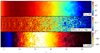Fig. 1. Slices through the Tradio (top), Pop III SFRD (middle), and T21 (bottom) lightcones for our illustrative model (see text for details). The simulation presented here has a box size of 5003 Mpc3 with a resolution of 2503. In order to accentuate the cosmic dawn era, we plot the horizontal axes linearly in redshift (as opposed to linearly in comoving scale).

We further quantify the above claims in Fig. 2. In the top-left and right panels we show the evolution of ${\overline{T}}_{21}$ and ${\overline{T}}_{\mathrm{radio}}$, respectively, where here and below we use $\overline{x}$ to denote globally averaged values of the physical quantity x. We see that indeed the 21 cm global signal in this model is comparable in amplitude and timing to the Maximum a Posteriori (MAP) flattened Gaussian model recovered by EDGES (dashed blue line in the top-left panel). It achieves this without exceeding the ARCADE2 radio background measurements (middle panel). The latest CMB data from the Planck 2018 measurements constrains the reionization optical depth τ_rei to be (see Qin et al. 2020b)

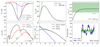Fig. 2. Summaries for the simulation shown in Fig. 1. In the top-left and middle panels, the black solid lines show global average values for T21 and Tradio, respectively. In the top-right panel, the black solid line shows the cumulative optical depth τrei(< z), which falls into the 95% C.I. region derived from Planck constraints in Eq. (31) (shown in green shaded contour). The blue dashed line in the ${\overline{T}}_{21}$ panel shows the MAP flattened Gaussian profile recovered by B18, while the red curve corresponds to the same astrophysical model as shown with the black curve but without a radio background excess. The radio background observed by ARCADE2 (see Eqs. (26, 39)) is indicated in the ${\overline{T}}_{\mathrm{radio}}$ panel with the green solid line. The lower left panel shows the 21 cm power spectrum at k = 0.1 Mpc−1, with black and red solid lines corresponding to the cases with and without a radio excess, respectively, the green dashed line represents the projected SKA noise power at k = 0.1 Mpc−1 with a 1000 hour integration taken from Barry et al. (2022). We show the global star formation rate density in the lower middle panel, where the blue, black and green solid lines represent contributions from Pop II galaxies, Pop III galaxies and their sum, respectively. In the lower right panel, we present the brightness temperature residuals (mean and 95% C.I.) after performing inference on EDGES data with a five-term FG model and fixing the cosmic signal to the ${\overline{T}}_{21}$ profile shown with the black solid line in the top-left panel. There is an obvious, unaccounted for signal remaining in these residuals. For comparison, we also show in this panel the noise-like mean from our highest evidence model (green solid line; see Sect. 9 for details).

$$\begin{array}{c}\hfill {\tau }_{\mathrm{rei}}=0.{0569}_{-0.0066}^{+0.0081}.\end{array}$$(31)

From the top-right panel of Fig. 2 it can be seen that our accumulative optical depth (defined as ${\tau }_{\mathrm{rei}}(<z)\equiv {\displaystyle {\int }_0^z}\frac{\mathrm{d}{\tau }_{\mathrm{rei}}}{\mathrm{d}z\prime }\mathrm{d}z\prime$) is consistent with current reionization constraints in Eq. (31). We recall that by construction, the model is consistent with Hubble observations of UV LFs at z ≳ 6, as these only constrain relatively bright Pop II galaxies whose values we fix to those in Muñoz et al. (2022).

The lower left panel of Fig. 2 shows the evolution of the large-scale (k = 0.1 Mpc⁻¹) 21 cm power spectrum (PS) Δ₂₁², defined as

$$\begin{array}{c}\hfill \langle {\stackrel{\sim }{T}}_{21}(k,z){\stackrel{\sim }{T}}_{21}^{\ast }(k\prime ,z)\rangle \equiv {(2\pi )}^3{\delta }_{(}k-k\prime )\frac{2{\pi }^2}{k^3}{\mathrm{\Delta }}_{21}^2(z,k),\end{array}$$(32)

where ${\stackrel{\sim }{T}}_{21}$ indicates the 3D Fourier transform of T₂₁⁴. The black curve corresponds to the fiducial model discussed in this section, while the red curve corresponds to the same model but assuming no radio background excess (i.e., f_R,III = 0). In both cases, the large-scale power exhibits the usual three peak evolution, marking (from left to right) the epochs of reionization (EoR), X-ray heating (epoch of heating, EoH) and Lyman-Alpha pumping (Pritchard & Furlanetto 2007; Mesinger et al. 2011; Lopez-Honorez et al. 2016). However, the addition of a population of radio loud Pop III galaxies enhances the peak amplitude of the large-scale power during the EoH by over an order of magnitude (see also Fialkov & Barkana 2019; Reis et al. 2020). The green dashed line corresponds to an estimate of the thermal noise power achievable with a 1000 h integration with SKA (Barry et al. 2022); such exotic signals should be easily observable by upcoming radio interferometers.

In the bottom-middle panel, we show the relative contributions to the total SFRD (green curve), provided by Pop II galaxies (blue curve) and Pop III galaxies (black curve). We see explicitly that Pop III galaxies in this model dominate the SFRD during the CD, at z ≳ 10. At lower redshifts, their SFRD starts to decrease due to a combination of LW feedback, photo-heating feedback and the evolution of the halo mass function (see Muñoz et al. 2022).

Based on the previously mentioned results, it would seem this Pop III radio background model can roughly reproduce the EDGES data, while being consistent with complementary observations. If we define a “pseudo-likelihood” using the timing and depth of the flattened Gaussian recovered by EDGES, we might conclude this model provides a good description of the data. However, our cosmic signal is not a flattened Gaussian, and we should define a likelihood directly in data space (i.e., the observed sky temperature).

To check how well this model actually reproduces the data, we perform an inference in which we fix the cosmic signal (black solid curve in the top-left panel), and sample a five-term log-polynomial FG (as in B18) using the likelihood defined by Eq. (36) (the details of our inference procedure are discussed in Sections 5 and 6). In the bottom-right panel of Fig. 2 we plot the mean and 95% C.I. of the resulting residual signal (i.e., data minus model). If the model were a complete description of the data, these residuals should just be zero mean Gaussian noise. However, there is clear structure in the residuals, and this is especially obvious when compared with the residual for our highest evidence model (green solid line, to be detailed in Sect. 9). Thus, despite the apparent agreement with the B18 flattened Gaussian in terms of ${\overline{T}}_{21}$ depth and timing, the model does not explain the data. We discuss this in more detail in Sect. 8 where we further quantify the dangers inherent in using a “pseudo-likelihood” defined on a flattened Gaussian summary of the data.

4.2. Impact of galaxy parameters

In Fig. 3 we visualize how essential aspects of Pop III astrophysics impact the 21 cm global signal and power spectrum. The black curve corresponds to the fiducial parameter combination discussed in the previous section, while the red (green) curves illustrate how each observable changes when decreasing (increasing) one parameter at a time in each column. The variations in Δ₂₁² largely follow those in ${\overline{T}}_{21}$, that is, an enhanced global signal provides an increased dynamic range resulting in more power on large spatial spaces. Below we summarize our Pop III galaxy parameters and their qualitative impact:

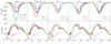Fig. 3. Effects of varying Pop III galaxy parameters on the 21 cm global signal (top) and power spectrum (bottom, at k = 0.1 Mpc−1). From left to right, we vary fR,III, LX,III < 2 kev, fesc,7, f⋆, 7 and ALW, respectively. The black solid lines correspond to the fiducial values used to compute Fig. 1, while the green (red) solid lines show the result from increasing (decreasing) each parameter while keeping the others fixed. The global 21 cm signal reported in B18 is shown in the top panels with blue dashed lines. In Δ212 panels the magenta dashed lines show the forecasted SKA sensitivity at k = 0.1 Mpc−1 (Barry et al. 2022).

(I) f_R,III – the radio luminosity to star formation rate for Pop III galaxies, normalized to values seen in local galaxies. Efficiencies of f_R,III ≳ 10²−10³ drive a radio background during the CD that exceeds that of the CMB. Increasing f_R,III in this regime deepens the absorption trough in the global signal and drives a corresponding increase in the power spectrum. The spin temperature is also coupled to T_radio via Eq. (30); therefore a higher f_R,III delays the coupling between T_S and T_k and thereby shifts the first peak of Δ₂₁² to lower redshifts.

(II) L_X,II < 2 kev – the bolometric X-ray luminosity per SFR of Pop III galaxies. Increasing L_X,III < 2 kev shifts the EoH to earlier times. Therefore the gas does not have as much time to cool before being heated, and the corresponding global absorption trough and peak in the power spectrum are reduced and shifted to earlier times.

(III) f_esc,7 – the escape fraction of ionizing photons from Pop III galaxies, normalized to halos with a mass of 10⁷ M_⊙. Increasing f_esc,7 increases the contribution of Pop III galaxies to the EoR. Shifting the EoR to earlier times reduces the depth of the absorption trough in the global signal. The corresponding overlap of the EoR and EoH dramatically reduces the late time PS, as the ionization-temperature cross terms become important (see Mesinger et al. 2014).

(IV) f_⋆,7 – the fraction of galactic gas in stars for Pop III galaxies, normalized to halos with a mass of 10⁷ M_⊙. Increasing f_⋆,7 increases star formation in early sources, shifting all cosmic epochs to earlier times. Because the radio background excess also scales with the star formation rate, the absorption trough deepens with increasing f_⋆,7.

(V) A_LW – the efficiency of LW feedback on star formation. Increasing A_LW makes it easier for a LW background to quench star formation in Pop III galaxies, which has a qualitatively similar impact as decreasing f_⋆,7.

In Fig. 3 we also show projected SKA power spectrum sensitivity with a 1000 hour integration (Barry et al. 2022), and we find that for each Δ₂₁² panel, variations of power spectrum induced by changing relevant parameters exceed the SKA sensitivity. Thus upcoming SKA data could constrain our model parameters within ranges adopted in Fig. 3.

5. Foreground and systematics nuisance parameters

The physically motivated FG model used in B18 was found to lack the flexibility required to capture the beam-weighted FGs of the observations (SP20). In this work, we use a more flexible FG model, as well as an extra term designed to mimic residual structure left over from calibration. We summarize them in details below.

5.1. Foreground model

The main contaminants of the cosmic 21 cm signal come from galactic FGs, which can be well parameterized by a power-law syncrotron spectrum, and the Earth’s ionosphere (Hills et al. 2018; Bowman et al. 2018b; Sims & Pober 2020). We model their overall contribution using a log-polynomial functional form following Murray et al. (2022),

$$\begin{array}{c}\hfill T_{=}{\left(\frac{\nu }{75\mathrm{MHz}}\right)}^b{\displaystyle \sum _{i=0}^{N_{-}1}}{p}_i{[ln\left(\frac{\nu }{75\mathrm{MHz}}\right)]}^i,\end{array}$$(33)

where ν denotes frequency, b is the frequency spectra index, N_FG is the total number of FG terms, and p_i are the polynomial coefficients. We vary the number of FG terms when maximizing the Bayesian evidence below.

5.2. Calibration residuals

Despite the monumental task undertaken by the EDGES team to understand their data pipeline, possible imperfections in the calibration process can result in residual systematics (Hills et al. 2018; Singh & Subrahmanyan 2019; Sims & Pober 2020). As these systematics are “unknown unknowns”, it is difficult to characterize their contribution via some basis and associated priors. Here we use the parametrization suggested by SP20. Specifically, we account for possible calibration systematics using a power-law damped sinusoid model,

$$\begin{array}{c}\hfill T_{=}{\left(\frac{\nu }{75\mathrm{MHz}}\right)}^b[a_{0}sin(2\pi \nu /P)+a_{1}cos(2\pi \nu /P)],\end{array}$$(34)

where a₀ and a₁ are amplitudes in Kelvin for the sine and cosine components, and P is the period in MHz. As noted in SP20, this model of calibration residuals is reasonably well motivated physically, and corresponds to a spectrally structured gain error in the calibration, which is weighted by the FG spectrum. Such systematics could in principle be generated by imperfect measurements of the reflection coefficients of the amplifier (Murray et al. 2022).

Motivated by studies of galactic synchrotron radiation (Mozdzen et al. 2017; Monsalve et al. 2021), we set b = −2.5 in Eq. (33) and Eq. (34), and we have checked that our results remain unchanged when allowing b to vary or when we adopt the alternative T_FG parameterization used in SP20. Furthermore, we find that our T_FG parameterization shows higher Bayesian evidence compared to model adopted in SP20.

6. Likelihoods

In addition to EDGES, we also use complementary observations from ARCADE2 and Planck, which allow us to disfavor models that explain the EDGES result by either reionizing the Universe too early or producing a radio background in excess of currently observed limits. Thus our final log-likelihood takes the form

$$\begin{array}{c}\hfill ln\mathcal{L}=ln{\mathcal{L}}_{+}ln{\mathcal{L}}_{+}ln{\mathcal{L}}_{\mathit{Planck}},\end{array}$$(35)

where the terms on the right hand side represent contributions from EDGES, ARCADE2 and Planck, respectively. We discuss each term below.

6.1. EDGES

We adopt a Gaussian form for the EDGES likelihood,

$$\begin{array}{c}\hfill ln{\mathcal{L}}_{=}-\frac{1}{2}{\displaystyle \sum [\frac{{(T_{\mathrm{sky}}-T_{\mathrm{model}})}^2}{{\sigma }_{\mathrm{T}}^2}+2ln{\sigma }_{\mathrm{T}}]}+\mathrm{const},\end{array}$$(36)

where the summation is over all weighed EDGES frequency bins, and we treat the Gaussian error σ_T as a free parameter to be varied in our inference. As discussed in Sect. 2, T_sky is the EDGES sky temperature data, and the theoretical model value T_model is a combination of the 21 cm signal ${\overline{T}}_{21}$, FG temperature T_FG, and residual calibration systematics T_cal,

$$\begin{array}{c}\hfill T_{=}{\overline{T}}_{21}+T_{+}{T}_{.}\end{array}$$(37)

6.2. ARCADE2

Our ARCADE2 likelihood penalizes models that produce radio excess above the observed level, which includes a contribution from galactic sources as well as a potential cosmological component. Since the measurement is therefore an upper limit on the cosmological component, we adopt a simple one-sided Gaussian form⁵:

$$\begin{array}{cc}\hfill ln{\mathcal{L}}_{\mathrm{ARCADE}2}& =-\frac{1}{2}{\displaystyle \sum \frac{{({\overline{T}}_{\mathrm{radio}}-T_{\mathrm{ARCADE}2})}^2}{{\sigma }_{\mathrm{ARCADE}2}^2}}\hfill \\ \hfill & \times \mathrm{\Theta }({\overline{T}}_{\mathrm{radio}}-T_{\mathrm{ARCADE}2})+\mathrm{const},\hfill \end{array}$$(38)

where the summation is performed over the simulated redshifts (3.8 < z < 36), Θ(x) is the Heaviside step function which equals unity for x > 0 and vanishes otherwise, T_ARCADE2 is the ARCADE2 excess level at 1.42 GHz and redshift z, which can be derived from Eqs. (26) and (27) as

$$\begin{array}{c}\hfill T_{\mathrm{ARCADE}2}=1.19(1+z){\left(\frac{v{\prime }_{21}}{1\mathrm{GHz}}\right)}^{-2.62},v{\prime }_{21}=\frac{1.42\mathrm{GHz}}{1+z}·\end{array}$$(39)

Following the justification detailed in Appendix B, we approximate the uncertainty as

$$\begin{array}{c}\hfill {\sigma }_{=}0.1T_{.}\end{array}$$(40)

6.3. Planck

To ensure that our reionization history remains consistent with the latest Planck 2018 constraints in Eq. (31), we constructed our Planck optical depth likelihood following the parameterization used in the 21CMMC inference package (Greig & Mesinger 2018),

$$\begin{array}{c}\hfill ln{\mathcal{L}}_{\mathit{Planck}}=-\frac{1}{2}\left[\frac{{({\tau }_{\mathrm{rei}}-{\tau }_{\mathrm{plk}})}^2}{{\sigma }_u{\sigma }_l+({\sigma }_u-{\sigma }_l)({\tau }_{\mathrm{rei}}-{\tau }_{\mathrm{plk}})}\right]+\mathrm{const},\end{array}$$(41)

where τ_plk = 0.0569, σ_u = 0.0081 and σ_l = 0.0066.

7. Inference methodology

7.1. Models

In our inference we vary five free parameters characterizing Pop III galaxies:

$$\begin{array}{c}\hfill \{f_{\mathrm{R},\mathrm{III}},L_{\mathrm{X},\mathrm{III}<2\mathrm{keV}},f_{\mathrm{esc},7},f_{\star ,7},A_{\mathrm{LW}}\}.\end{array}$$(42)

Our cosmological model and associated prior ranges are fixed, and we explore several models varying combinations of: (i) polynomial order for FG parameters (from 4th–10th order); and (ii) inclusion of sinusoidal calibration residuals (with or without residuals). These combinations yield a total of 14 models, which are then compared using the Bayesian evidence. We summarize all free parameters and their prior ranges in Table 1, and we note that our priors for σ_T and T_cal are set following SP20.

Inference for each of these models varies 10–19 parameters and takes between 0.4 M to 60 M likelihood calls depending on the model complexity. For computational convenience, in all our inferences and relevant post-processing, we calculate ${\overline{T}}_{21}$, ${\overline{T}}_{\mathrm{radio}}$, τ_rei and Δ₂₁² using the 21cmEMU emulator. We train this emulator on a total of 1.3 × 10⁵ 21cmFAST outputs. After training, the emulator error on the output is orders of magnitude smaller than the corresponding observational uncertainty and is therefore negligible. The details of the training process and the dataset are provided in Appendix A.

7.2. Model comparison using the Bayesian evidence

For a model ℳ characterized by a set of parameters θ, Bayes theorem states that given the data D, the posterior probability distribution of θ is given by

$$\begin{array}{c}\hfill P(\mathit{\theta }|D,\mathcal{M})=\frac{\mathcal{L}(D|\mathcal{M},\mathit{\theta })\pi (\mathit{\theta }|\mathcal{M})}{\mathcal{Z}(D|\mathcal{M})},\end{array}$$(43)

where ℒ and π are likelihood and prior, respectively, and the Bayesian evidence 𝒵 is given by

$$\begin{array}{c}\hfill \mathcal{Z}(D|\mathcal{M})={\displaystyle \int \mathcal{L}}(D|\mathcal{M},\mathit{\theta })\pi (\mathit{\theta })\mathit{\theta }.\end{array}$$(44)

For parameter inference, the Bayesian evidence is simply a constant serving to normalize the posterior probability density, P, and can therefore be neglected. However, in the presence of different models or prior distributions, the relative evidences quantify the degree by which our prior model odds are changed by the data (see e.g., Trotta 2008). Denoting by π(ℳ_i) the prior probability for model ℳ_i, the posterior odds between two models ℳ_i, ℳ_j is given by

$$\begin{array}{c}\hfill \frac{P({\mathcal{M}}_i|D)}{P({\mathcal{M}}_j|D)}=\frac{Z_i}{Z_j}\frac{\pi ({\mathcal{M}}_i)}{\pi ({\mathcal{M}}_j)}·\end{array}$$(45)

The ratio of evidences is called the Bayes factor, B_ij = Z_i/Z_j, and it incorporates a quantitative notion of Occam’s razor: a model is preferred (i.e., has a larger Bayesian evidence) when it explains the data better (i.e., it achieves a larger maximum likelihood) with an economy of free parameters. Therefore, a model that can better reproduce the data (having a higher likelihood) and is more predictive (having a smaller number of free parameters or more constrained prior ranges compared to the posterior) results in a correspondingly higher Bayesian evidence. When comparing between models ℳ₁ and ℳ₂, we follow Jeffreys (1998), Kass & Raftery (1995) and use ln𝒵₁/𝒵₂ > 4.6 as ‘decisive’ preference of ℳ₁ over ℳ₂. In our analysis below, we assume a flat prior over all models; therefore the posterior odds between two models reduces to the corresponding Bayes factor.

7.3. Nested sampling with MultiNest

Inferences in this work are performed using the MultiNest (Feroz et al. 2009; Buchner et al. 2014) package. MultiNest uses nested sampling (Skilling 2004) to efficiently calculate the Bayesian evidence and parameter posteriors. We use default parameter choices, except for the number of live points (N_live), which we set to 100n_dim in our fiducial inferences, where n_dim is the dimensionality of model parameter space. We analyze the MultiNest output using the GetDist (Lewis 2019) package to derive posteriors for model parameters and associated observables (e.g., ${\overline{T}}_{21}$, ${\overline{T}}_{\mathrm{radio}}$), which are treated as derived parameters of our model. We confirm that the posteriors have converged for the above choices.

8. Using a “pseudo-likelihood” based on a backward-modeled flattened Gaussian

Before showing inference results of self-consistent forward-modeling of the EDGES sky temperature, here we construct the likelihood on the recovered (MAP) flattened Gaussian from B18. This serves to mimic the common approach in the literature (e.g., Mirocha & Furlanetto 2019; Fialkov & Barkana 2019; Ewall-Wice et al. 2020; Reis et al. 2020), in which a physical cosmological model is compared with a recovered empirical profile (flattened Gaussian), without directly forward-modeling the observed data.

Specifically, we follow Mirocha & Furlanetto (2019) and construct a Gaussian pseudo-likelihood of the form

$$\begin{array}{c}\hfill ln\mathcal{L}=-{\displaystyle \sum _{\frac{{(T_{-}{\overline{T}}_{21,})}^2}{2{\sigma }^2}}}+\mathrm{const},\end{array}$$(46)

where the summation is over all lightcone redshifts within EDGES frequencies, T_B18 is the flattened-Gaussian profile reported in B18, we assume that different redshifts are independent and set the uncertainty σ to 100 mK.

In the first three panels of Fig. 4 we show the posteriors for ${\overline{T}}_{21}$, ${\overline{T}}_{\mathrm{radio}}$ and ${\overline{x}}_{\mathrm{H}}$ using this pseudo-likelihood. We adopt the priors in Table 1 for results shown in red (hereafter dubbed Wide f_⋆,7). From the ${\overline{T}}_{21}$ and ${\overline{T}}_{\mathrm{radio}}$ panels we see that our model can roughly recover the B18 result without invoking an ad-hoc “z_off” parameter to turn off the radio and (or) X-rays from the first galaxies (Mirocha & Furlanetto 2019; Reis et al. 2020; Sikder et al. 2024a,b). Self-consistently modeling the feedback on Pop III galaxies is able to physically turn off this population so that their radio background does not exceed the ARCADE2 observations.

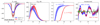Fig. 4. Results from our pseudo-likelihood inferences in which the likelihood is defined on the recovered flattened Gaussian from B18 instead of directly in the sky temperature space (see text for details). Our ARCADE2 and Planck likelihoods are also included in the analysis. From left to right, we show in red and blue the posteriors for ${\overline{T}}_{21}$, ${\overline{T}}_{\mathrm{radio}}$, ${\overline{x}}_{\mathrm{H}}$ and the residuals. Solid and dashed lines correspond to mean and MAP, respectively, and shaded contours indicate 95% C.I.s. Results in red use the astrophysical prior ranges listed in Table 1 and lead to an extremely early reionization. Those in blue adopt a narrow fesc,7 prior of [10−6, 10−2.5] to accommodate EoR timing constraints. In the ${\overline{T}}_{21}$ panel, we show B18 profile with black solid line and gray shaded region represents the uncertainty level adopted in our Pseudo-likelihood. The black solid line in the ${\overline{T}}_{\mathrm{radio}}$ panel shows the ARCADE2 excess. The 95% C.I. on τrei are indicated in the ${\overline{x}}_{\mathrm{H}}$ panel. For the residuals panel, we fit the EDGES data with a five term FG model while fixing the cosmic 21 cm signal to the corresponding MAP results in ${\overline{T}}_{21}$ panel. There is clear structure in the residuals. For comparison, we also include the residuals from our highest evidence model as a green line, which are noise-like.

However, the recovered optical depth for the above inference is significantly higher than inferred from Planck data. This is due to the fact reionization can provide a more rapid rise in the global signal at z ≲ 18 compared with X-ray heating. The improved agreement with the flattened Gaussian pseudo-likelihood is enough to exceed the corresponding penalty from the Planck likelihood. To accommodate Planck optical depth constraints (see Eq. (31)), we also perform inference restricting the prior range on the escape fraction f_esc,7. Specifically, posterior in blue corresponds to a tighter log-uniform f_esc,7 prior of [10⁻⁶, 10^−2.5] (dubbed as Narrow f_esc,7 hereafter). The recovered ${\overline{T}}_{21}$ posterior of the Narrow f_esc,7 model is a lot less narrow compared to the Wide f_esc,7 model. Without reionization at z ∼ 16, the rise in the global 21 cm signal is limited by the (comparably less efficient) EoH and is therefore slower.

The last panel of Fig. 4 shows the residuals from fitting the EDGES data with only a 5 term FG while fixing ${\overline{T}}_{21}$ to the MAP results from our pseudo likelihood fits. The red and blue contours indicate 95% C.I. regions for model using ${\overline{T}}_{21}$ from Wide f_esc,7 and Narrow f_esc,7 set-ups, respectively. If the combination of fixed cosmic signal and FG did describe the EDGES data, one would expect the residuals to be noise-like. However it can be seen that the residuals show oscillating structures that are not consistent with noise, especially when compared with that of our highest evidence model (green dashed line, detailed in Sect. 9). This indicates that the combination of FG and fixed B18-like cosmic signal (inferred from the pseudo-likelihood) does not give a reliable description to the actual EDGES data. We therefore conclude that for physical models, one cannot use a likelihood based on summaries of the recovered flattened Gaussian.

9. Results

We now show our main results, in which we forward-modeled the full EDGES sky temperature data, constructing the likelihood directly in data space as discussed in Sect. 7. In Fig. 5 we show the Bayesian evidence ratios normalized to the highest evidence model with 𝒵 = 𝒵_max, which features 7 FG terms and calibration residuals. From left to right, in each panel we show results respectively as a function of (i) the number of FG terms, (ii) ${\overline{T}}_{21}$ at redshift 17, and (iii) the calibration amplitude A_cal (defined as $\sqrt{a_0^2+a_1^2}$). In the middle panel, the gray shaded region indicates the regime of ${\overline{T}}_{21}<-210$ mK, corresponding to models with a radio background in excess of the CMB. For simplicity, hereafter we refer to regimes with and without radio excess as non-standard and standard, respectively.

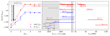Fig. 5. Bayesian log-evidence normalized to the highest evidence model, $ln{\mathcal{Z}/\mathcal{Z}}_{\max }$, as a function of FG flexibility NFG (squares in the left panel), ${\overline{T}}_{21}$ at z = 17 (middle), and calibration amplitude Acal (right, defined as $A_{\mathrm{cal}}\equiv \sqrt{a_0^2+a_1^2}$). Models with NFG ≥ 9 are omitted in the middle and right panel for visibility, as they overlap with NFG = 8, 9. Models below the horizontal gray dashed line are decisively disfavored ($ln{\mathcal{Z}/\mathcal{Z}}_{\max }\le -4.6$). We use red and blue colors to represent scenarios of no Tcal and with Tcal , respectively. The error bars in the middle and right panels represent 95% C.I. regions around the mean. In the middle panel, the region below the standard expectation (${\overline{T}}_{21}<-210$ mK) is shaded in gray, while the vertical black dashed line indicates ${\overline{T}}_{21}=0$. In the left panel, the blue and red crosses show the maximum log-likelihood ratio, $ln(\widehat{\mathcal{L}}/{\widehat{\mathcal{L}}}_{\star })$, normalized to our highest evidence model.

As can be seen from the left panel, the Bayesian evidence peaks at N_FG = 7 for both calibration settings. On the same plot, we also display the maximum log-likelihood value for each model, normalized to the maximum log-likelihood of the highest evidence model (blue and red crosses). We observe that the maximum log-likelihood increases monotonically with the number of free parameters, as expected, but that the slope decreases sharply at N_FG = 7. This indicates that the sharp increase in log-evidence until N_FG = 7 is a reflection of the increasing quality of fit of models with more FG free parameters. After N_FG = 7, however, adding extra freedom to the model results in an Occam’s razor penalty in the evidence, which manifests as a decrease in its value. In fact the only model that is not decisively disfavored in comparison to the highest evidence model is one with N_FG = 8 and calibration error. Thus calibration errors are needed to explain the data in the context of our physical model.

The middle panel of Fig. 5 shows that at z = 17 (i.e., the central redshift of the putative cosmic signal recovered by B18), only models with N_FG ≤ 5 have a preference for a radio background excess. Adding more FG terms disfavors non-standard ${\overline{T}}_{21}$ amplitudes and increases the Bayesian evidence. For example, at N_FG = 4, ${\overline{T}}_{21}$ amplitudes at z = 17 are constrained to [−1482, −1183] mK, with corresponding log-evidence ratios between −199 and −179. In contrast, posteriors for all N_FG ≥ 6 models lie exclusively in the standard range of [ − 210, 30] mK.

In the right panel of Fig. 5, we find that inflexible FG models (N_FG ≤ 5) paired with our 21 cm model are wildly insufficient to account for the data, and the calibration residuals are required to be very large (A_cal ∼ 103 mK). As the number of FG terms are increased, some of the higher-order residual structure that was fit by the calibration-residual term is accounted for by the FGs, and the calibration-residual amplitude required reduces to A_cal ∼ 51 mK for the high-evidence models.

In Fig. 6 we show additional observables from these models. The columns correspond to ${\overline{T}}_{21}$, ${\overline{T}}_{\mathrm{radio}}$, ${\tau }_{\mathrm{rei}}(<z)\equiv {\displaystyle {\int }_0^z}\frac{\mathrm{d}{\tau }_{\mathrm{rei}}}{\mathrm{d}z\prime }\mathrm{d}z\prime$, and the associated residuals from the EDGES observation, from left to right. Each row corresponds to a different model, following the general trend of increasing prior volume with decreasing row. The top subsection includes models without calibration residuals, while models in the bottom subsection include calibration residuals. In both we show models with N_FG = 4−8. In each subpanel, the mean and 95% C.I. are indicated with black solid curves and blue shaded contours. The green shaded contours in the ${\overline{T}}_{21}$ subpanels correspond to the 95% C.I. of “standard models” without a radio excess (i.e., obtained by setting f_R,III to zero and using only the Planck likelihood term). The gray shaded regions in the same panels correspond to the 95% C.I. using only the ARCADE2 and Planck likelihood terms (i.e., without EDGES). In the ${\overline{T}}_{\mathrm{radio}}$ and τ_rei subpanels, we also show the ARCADE2 radio excess (see Eq. (39)) and the Planck 95% C.I. constraint (derived from Eq. (41)) with magenta lines and green shaded regions, respectively.

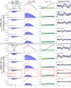Fig. 6. Marginalised posteriors from a subset of our inferences. From left to right, we show results for ${\overline{T}}_{21}$, ${\overline{T}}_{\mathrm{radio}}$, cumulative optical depth τrei(z), residual ($T_{\mathrm{sky}}-{\overline{T}}_{21}-T_{\mathrm{FG}}-T_{\mathrm{cal}}$), respectively. Each row corresponds to a different model, with the general trend of increasing systematics prior volume with decreasing row. The number of FG terms NFG is indicated in the y-axis in the ${\overline{T}}_{21}$ sub-panels. Black solid lines and blue shaded contours show mean and 95% C.I. regions, respectively. In the ${\overline{T}}_{21}$ sub-panels, the green contours indicate the 95% C.I. assuming no radio background excess (i.e., setting fR,III = 0 and only using the Planck likelihood), while the gray contours indicate the 95% C.I. using only ARCADE2 + Planck likelihoods (i.e., no EDGES). The green bar in the τrei(z) sub-panels denotes the 95% C.I. from Planck (Qin et al. 2020b) (see Eq. (31)). In the residual sub-panels, the ±2σ extent of the inferred Gaussian error σT is demarcated in gray.

As can be seen from the right-most column, the amplitude and the level of coherent (not noise-like) structure of the residuals decrease as we increase the prior volume of the systematics terms. All models that do not include calibration errors (first five rows) have visible structure in the residuals. In order not to have structure in the residuals, we require N_FG ≥ 7 AND calibration errors (bottom two rows). This again highlights that our physical model for the extra radio background, contrary to the ad-hoc flattened Gaussian, is unable to explain the EDGES signal by itself.

As was already noted in Fig. 5, the only models that prefer a non-standard depth for ${\overline{T}}_{21}$ are those with N_FG ≤ 5. Interestingly, these models require a very early reionization. This is because reionization can provide a more rapid rise in the global signal at z ≲ 18 compared with X-ray heating. The improved agreement with the EDGES data from such a rapid rise compensates for its worse agreement with Planck. Regardless, these models do not actually explain the EDGES data, as can be seen visually from the structure in the residuals and as is quantified by the Bayesian evidence.

In red we highlight our highest evidence model, which includes seven FG terms as well as calibration errors. We see that the radio background and the CMB optical depth of this model are consistent with observations. Moreover, the global signal residuals in the rightmost panel are noise-like. Interestingly though, the posterior of the global signal seems perfectly aligned with the “no radio excess” posterior in green. Indeed, this claim holds true for all models with N_FG ≥ 6. This implies that higher order FG terms (and systematics errors) do a better job of reproducing the EDGES signal than our physical, excess radio background model.

We investigate this claim further in Fig. 7, showing the probability distribution function (PDF) of ${\overline{T}}_{21}$ at redshift 17, for our maximum evidence model (a corner plot for this model is shown in Appendix C). Non-standard depths are demarcated with the gray shaded region. The black line corresponds to our astrophysical prior, and is generated using 3.2 × 10⁶ samples. The other lines show posterior PDFs using different likelihood combinations, as indicated in the figure legend. For these, we increase N_live = 500n_dim, confirming that the posterior in the tails of the distribution has converged.

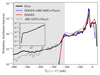Fig. 7. Probability distribution functions for ${\overline{T}}_{21}$ at z = 17 from our highest evidence model. The black curve corresponds to our prior distribution, while the other curves correspond to posterior PDFs obtained using various likelihood terms as denoted in the legend. The gray shaded region marks the regime of non-standard depths. The inset shows the prior extended to very low temperatures.

Roughly 17% of our prior samples have non-standard depths (black curve). There is not much difference between the black and gray curves, showing that ARCADE2 and Planck do not have much impact on our prior in this space⁶. However, when we include also the EDGES likelihood (blue curve), the posterior PDF shifts to disfavor non-standard models. Roughly the same result is obtained if we only consider the EDGES data (red curve). This figure shows that, not only does our radio excess model fail in explaining EDGES, it actually interferes with the systematics terms that do a better job. In other words, the EDGES data disfavors a non-standard radio background during the Cosmic Dawn. This is qualitatively contrary to previous conclusions, highlighting the inherent dangers of using a pseudo-likelihood built on a model (flattened Gaussian) that is different from the one being used in the inference (Mirocha & Furlanetto 2019; Fialkov & Barkana 2019; Reis et al. 2020; Ewall-Wice et al. 2020).

10. Discussion and caveats

Other works have also performed Bayesian analysis on EDGES data in order to further test the B18 result (e.g., Hills et al. 2018; Singh & Subrahmanyan 2019; Sims & Pober 2020; Tauscher et al. 2020; Murray et al. 2022). Most, however, perform inference with a flattened Gaussian, or use the flattened Gaussian to define a pseudo-likelihood (Mirocha & Furlanetto 2019; Fialkov & Barkana 2019; Ewall-Wice et al. 2020; Reis et al. 2020); Mebane:2020jwl. Closest to our analysis was SP20 in which the authors compared Bayesian evidences of multiple models for the cosmic signal, FGs, calibration residuals and Gaussian noise (σ_T of our EDGES likelihood in Eq. (36)). They concluded that the EDGES signal could be explained either with a phenomenological flattened Gaussian with a non-standard depth or with calibration residuals. Their physical models for the cosmic signal (computed with the ARES code; Mirocha 2014) did not include a radio background excess. Here we show that a physical model for the radio background excess, as opposed to a phenomenological flattened Gaussian, is actually disfavored by EDGES data.

While we have shown for our specific cosmological model that EDGES intrinsically disfavors a non-standard ${\overline{T}}_{21}$ depth, we expect a similar result for any physical model anchored on galaxy evolution. Though EDGES data has been shown to give non-standard depth for the phenomenological flat Gaussian ${\overline{T}}_{21}$ model (see e.g., B18 and the updated analysis in Murray et al. 2022), there are two unusual features of such a profile that cannot be simultaneously mimicked by realistic astrophysical models: the flatness of the trough and the sharpness of the wings.

All realistic cosmological explanations of the EDGES signal require galaxies and (or) black holes to play a role during the cosmic dawn (e.g., Mirocha & Furlanetto 2019; Reis et al. 2020; Ewall-Wice et al. 2020). The redshift evolution of galaxies is linked to the well-known evolution of the halo mass function, which cannot mimic the sharp features of the flattened Gaussian shape reported in B18 while maintaining the consistency with other astrophysical constraints. Kaurov et al. (2018) suggested that the sharpness can be reproduced if Lyman-alpha coupling between spin and kinetic temperatures were driven by halos with masses in excess of ∼10^9 − 10 M_⊙, and assuming a constant mass to light ratio. However, there is no known physical mechanism to quench star formation in smaller halos at z > 18; moreover, we know from observed UV LFs that galaxies do not have constant mass to light ratios (see e.g., Bromm 2013; Mesinger et al. 2011). Even with these caveats, such a model for a steep evolution of the global signal does not result in a flattened shape.

The flatness in the flattened Gaussian shape could be achieved if there are multiple IGM heating sources that are very precisely tuned so that their combination heats the gas temperature as T_K ∝ (1 + z). IGM heating that is comparable to that provided by X-rays could be achieved in some models of dark matter decay (e.g., Facchinetti et al. 2024; Sun et al. 2025), annihilation (e.g., Valdés et al. 2013; Evoli et al. 2014; Lopez-Honorez et al. 2016; Cang et al. 2023) and cosmic rays (e.g., Leite et al. 2017; Gessey-Jones et al. 2023). Such a multiple heating scenario was in fact suggested by Gessey-Jones et al. (2023), in which the authors implemented both X-ray and cosmic ray heating (see their Fig. 10). However this requires extreme fine-tuning of astrophysics in order to achieve such a precise evolution, in addition to the already exotic assumption of a radio background excess; thus the Bayesian evidence of such models would be strongly penalized by the small prior volume of viable parameters. Moreover, even with a relatively flat evolution resulting from such astrophysical “tuning”, a double heating scenario is unable to achieve the sharpness of the flattened Gaussian MAP from B18, as also pointed out in Gessey-Jones et al. (2023).

Finally we point out that our results also depend on our specific model and associated prior volume for FGs and systematics. As mentioned earlier, both of these are physically motivated. However, our understanding of systematics is far from complete. With an improved characterization of FG + calibration residuals resulting in a more physical basis and (or) prior volume, our conclusions could change.

11. Conclusions

The existence of a radio background at z ∼ 17 in excess of the CMB provided a popular explanation for the strong global 21 cm signal reported by the EDGES collaboration (e.g., Feng & Holder 2018; Ewall-Wice et al. 2018, 2020; Sharma 2018; Fialkov & Barkana 2019; Mirocha & Furlanetto 2019; Reis et al. 2020; Mebane et al. 2020; Ziparo et al. 2022; Sikder et al. 2024a,b; Zhang et al. 2023). This work investigates the radio excess from the first generation Pop III galaxies. These galaxies are naturally sterilized at lower redshifts due to LW and photoheating feedback, and thus can reproduce the EDGES absorption depth without violating upper limits on the radio background from ARCADE2.

We demonstrate that Pop III radio galaxies can indeed drive a 21 cm absorption signal that has the same depth and timing of the phenomenological flattened Gaussian recovered by EDGES, without violating constraints from complimentary observations. We perform Bayesian inference on EDGES sky temperature data, together with constraints from ARCADE2 and Planck. Our models for the sky temperature consist of the cosmic signal combined with FG and calibration errors of varying complexity. We compare these models using their Bayesian evidence.

Models that do not account for calibration errors are decisively disfavored by the data, showing clear structure in the residuals (i.e., the difference between the observed and forward-modeled sky temperature). Our highest evidence model is characterized by seven log-polynomial FG terms and calibration residuals. All models that have “noise-like” residuals and are not decisively disfavored by the EDGES data have posteriors consistent with standard model predictions (i.e., without a radio background excess). We show that not only does our radio excess model fail in explaining EDGES, but that excess radio backgrounds that produce beyond-standard absorption depths actually interfere with systematics models that do a better job.

Our conclusion that EDGES disfavors a strong cosmic 21 cm signal is different from all previous works that simulated a radio background excess. This difference stems from the fact that here we forward-model the EDGES temperature data directly and use a physical model for the cosmic 21 cm signal. Previous analyses that included physical models for the excess used a “pseudo-likelihood” based on a different model (the phenomenological flattened Gaussian). Our work therefore serves to highlight the importance of self-consistent inference.

Data Availability

We make our simulation code⁷ and associated emulator⁸ publicly available.

Acknowledgments

The authors gratefully acknowledge the HPC RIVR consortium and EuroHPC JU for funding this research by providing computing resources of the HPC system Vega at the Institute of Information Science (project EHPC-REG-2022R02-213). We thank Peter Sims, James Davis and Ivan Nikolić for helpful discussions. J.C. acknowledges support by SNS and the China Scholarship Council. A.M. and R.T. acknowledge support from the Ministry of Universities and Research (MUR) through the PRIN project “Optimal inference from radio images of the epoch of reionization”, the PNRR project “Centro Nazionale di Ricerca in High Performance Computing, Big Data e Quantum Computing”, and the PRO3 Scuole Programme ‘DS4ASTRO’. This project has received funding from the European Union’s Horizon 2020 research and innovation programme under the Marie Skłodowska-Curie grant agreement No 101067043. Y.Q. is supported by the ARC Discovery Early Career Researcher Award (DECRA) through fellowship #DE240101129.

References

Appendix A: Emulating the cosmic signal with 21cmEMU

The database used in our training consists of 1.3 × 10⁵ 21cmFAST simulations, distributed within our prior regions of astrophysical parameters (see Table 1). Samples are generated with our customized version of 21cmFAST and span a redshift range of z ∈ [3.8, 36], with a box of size 500 Mpc and a resolution of 50³ (which we find is sufficient for convergence in all of our observables to better than ∼ few percent). This database is then split into training, validation and test sets, each containing 10⁵, 10⁴ and 10⁴ samples, respectively. The network has a tree-like architecture where the input is passed into separate branches that each output the prediction for one of ${\overline{T}}_{21}$, ${\overline{T}}_{\mathrm{radio}}$, ${\overline{x}}_{\mathrm{H}}$, τ_rei and Δ₂₁². In Table A.1, we illustrate the number of layers and the number of neurons per layer for ${\overline{T}}_{21},{\overline{T}}_{\mathrm{radio}}$ and τ_rei branches, the results of which enter directly into our likelihoods.

We implement the emulator using PyTorch (Paszke et al. 2019). After training the emulator, we evaluate it against a test set. To measure its performance, we calculate the fractional error (FE):

$$\begin{array}{cc}& \mathrm{Abs}\mathrm{Diff}\equiv |{\mathrm{y}}_{\mathrm{true}}-{\mathrm{y}}_{\mathrm{pred}}|,\hfill \end{array}$$(A.1)

$$\begin{array}{cc}& \mathrm{FE}(\%)\equiv \frac{\mathrm{Abs}\mathrm{Diff}}{max(|{\mathrm{y}}_{\mathrm{true}}|,{\mathrm{y}}_{\mathrm{floor}})},\hfill \end{array}$$(A.2)

where y_true refers to the 21cmFAST simulation output and y_pred is the corresponding emulator prediction. In the last two rows of Table A.1, we show the mean FE as well as its 68% C.I. limit for each summary. We see that the brightness and radio temperatures have a mean FE of about 4%, while the neutral fraction and reionization optical depth have a mean FE of less than one percent. These emulator errors are orders of magnitude smaller than the observational uncertainty and are thus negligible.

Appendix B: Uncertainty level for ARCADE2 radio excess temperature

Our choice for the uncertainty level σ_ARCADE2 in Eq. (38) is well motivated by Bayesian analysis. The current radio brightness temperature measurements reported by ARCADE2 (Fixsen et al. 2011) can be expressed as the sum of temperatures of CMB T_CMB and radio excess T_excess,

$$\begin{array}{c}\hfill T=T_{\mathrm{CMB}}+T_{\mathrm{excess}},\end{array}$$(B.1)

and T_excess can be parameterized by a power-law,

$$\begin{array}{c}\hfill T_{\mathrm{excess}}=T_{\mathrm{r}}{\left(\frac{\nu }{\mathrm{GHz}}\right)}^{\beta }.\end{array}$$(B.2)

We treat T_CMB, T_r and β as free model parameters and derive their posterior distributions by sampling the following likelihood using MultiNest (Feroz et al. 2009; Buchner et al. 2014),

$$\begin{array}{c}\hfill ln\mathcal{L}=-\frac{1}{2}{\displaystyle \sum _i}\frac{T_{\mathrm{i}}-T_{\mathrm{data},\mathrm{i}}}{{\sigma }_{\mathrm{i}}^2}+const\end{array}$$(B.3)

where the subscript i indicates frequency, T_i is given in Eq. (B.1), the data T_data, i and uncertainty σ_i are taken from Table 4 of Fixsen et al. (2011).

Our inference constrains the model parameters to T_CMB = 2.730 ± 0.004K, T_r = 1.198 ± 0.129K and β = −2.613 ± 0.042 (uncertainties represents 68% C.I.), which is in almost identical agreement with values quoted in Fixsen et al. (2011).

Note that the excess level in Eq. (B.2) was given for z = 0. At 21cm frequency and arbitrary redshift z, the relevant excess level can be expressed as

$$\begin{array}{c}\hfill T_{\mathrm{excess},\mathrm{z}}=(1+z)T_{\mathrm{excess}}({\nu }_{21}^{\prime }),{\nu }_{21}^{\prime }=\frac{1.42\mathrm{GHz}}{1+z},\end{array}$$(B.4)

which is determined by model parameters T_r and β following Eq. (B.2). The posterior distributions for T_excess, z can be easily derived by analyzing the MultiNest inference chains for T_r and β.

In Fig. B.1, we show the MAP and 68% C.I. region for T_excess, z with black solid line and blue shaded region, respectively. It can be seen that, at 1 sigma (68%) credible interval, the upper bound on T_excess, z exhibits roughly 10% deviation relative to the MAP value. Therefore in our ARCADE2 likelihood, we set the uncertainty level σ_ARCADE2 to 10% of the MAP T_excess, z.

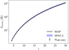Fig. B.1. Posteriors of radio excess level inferred from ARCADE2 datasets, the black solid curve shows the MAP results, and blue filled contour shows the 68% C.I. region, the black error bars show the error σARCADE2 used for our ARCADE2 likelihood in Eq. (38).

Appendix C: Parameter posteriors

In Fig. C.1 we present the posteriors for astrophysical parameters and derived ${\overline{T}}_{21}$ at z = 17 for 3 representative inference models: the highest evidence model (7 FG terms, with calibration residuals), the lowest evidence model (4 FG terms, no calibration residuals), and the Narrowf_esc, 7 pseudo-likelihood model from Sect. 8.

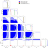Fig. C.1. One- and two-dimensional marginal posteriors for our astrophysical parameters and derived ${\overline{T}}_{21}$ at z = 17 resulting from different inferences. The plotted parameter ranges corresponds to their respective prior ranges. Blue and red contours and curves show results for our highest evidence model (seven FG terms, with calibration residuals) and lowest evidence model (four FG terms, no calibration residuals), respectively. Posteriors for the Narrowfesc, 7 pseudo likelihood inference from Appendix A are shown in green. Dark and light shaded contours represent 68% and 95% confidence intervals, respectively. The headings above the panels show 95%C.I. for the highest evidence model.

In the lowest evidence and pseudo-likelihood models, both of which have non-standard ${\overline{T}}_{21}$ depths, the relevant parameters are tightly constrained. Specifically, f_R, III is constrained to f_R, III ≳ 10^2.7, which also marks the minimum radio efficiency required for Pop III radio excess background to cause noticeable deviation of ${\overline{T}}_{21}$ from the standard regime. Both models adjust the cosmic signal timing to match that of B18 either through ionization (f_esc, 7) or heating (L_{X, III < 2keV}). In the lowest evidence model, timing and sharp rise of ${\overline{T}}_{21}$ are adjusted via increased ionization, and the f_esc, 7 posterior peaks close to our prior upper bound of 10⁻¹, resulting in an optical depth of τ_rei = 0.165. Whereas in the pseudo-likelihood for which a high f_esc, 7 is not viable due to the prior, a higher L_{X, III < 2keV} is required in order to match B18 timing.

In comparison, for our highest evidence model, EDGES data structure is mostly explained by FG and calibration systematics rather than the cosmic signal. Thus the constraints on astrophysical parameters are very weak. Since EDGES data intrinsically disfavors a strong non-standard ${\overline{T}}_{21}$ signal, we only recover upper limits on f_R, III and f_⋆, 7.

All Tables

All Figures

	Fig. 1. Slices through the Tradio (top), Pop III SFRD (middle), and T21 (bottom) lightcones for our illustrative model (see text for details). The simulation presented here has a box size of 5003 Mpc3 with a resolution of 2503. In order to accentuate the cosmic dawn era, we plot the horizontal axes linearly in redshift (as opposed to linearly in comoving scale).
In the text

Fig. 2. Summaries for the simulation shown in Fig. 1. In the top-left and middle panels, the black solid lines show global average values for T21 and Tradio, respectively. In the top-right panel, the black solid line shows the cumulative optical depth τrei(< z), which falls into the 95% C.I. region derived from Planck constraints in Eq. (31) (shown in green shaded contour). The blue dashed line in the ${\overline{T}}_{21}$ panel shows the MAP flattened Gaussian profile recovered by B18, while the red curve corresponds to the same astrophysical model as shown with the black curve but without a radio background excess. The radio background observed by ARCADE2 (see Eqs. (26, 39)) is indicated in the ${\overline{T}}_{\mathrm{radio}}$ panel with the green solid line. The lower left panel shows the 21 cm power spectrum at k = 0.1 Mpc−1, with black and red solid lines corresponding to the cases with and without a radio excess, respectively, the green dashed line represents the projected SKA noise power at k = 0.1 Mpc−1 with a 1000 hour integration taken from Barry et al. (2022). We show the global star formation rate density in the lower middle panel, where the blue, black and green solid lines represent contributions from Pop II galaxies, Pop III galaxies and their sum, respectively. In the lower right panel, we present the brightness temperature residuals (mean and 95% C.I.) after performing inference on EDGES data with a five-term FG model and fixing the cosmic signal to the ${\overline{T}}_{21}$ profile shown with the black solid line in the top-left panel. There is an obvious, unaccounted for signal remaining in these residuals. For comparison, we also show in this panel the noise-like mean from our highest evidence model (green solid line; see Sect. 9 for details).

In the text

Fig. 3. Effects of varying Pop III galaxy parameters on the 21 cm global signal (top) and power spectrum (bottom, at k = 0.1 Mpc−1). From left to right, we vary fR,III, LX,III < 2 kev, fesc,7, f⋆, 7 and ALW, respectively. The black solid lines correspond to the fiducial values used to compute Fig. 1, while the green (red) solid lines show the result from increasing (decreasing) each parameter while keeping the others fixed. The global 21 cm signal reported in B18 is shown in the top panels with blue dashed lines. In Δ212 panels the magenta dashed lines show the forecasted SKA sensitivity at k = 0.1 Mpc−1 (Barry et al. 2022).

In the text

Fig. 4. Results from our pseudo-likelihood inferences in which the likelihood is defined on the recovered flattened Gaussian from B18 instead of directly in the sky temperature space (see text for details). Our ARCADE2 and Planck likelihoods are also included in the analysis. From left to right, we show in red and blue the posteriors for ${\overline{T}}_{21}$, ${\overline{T}}_{\mathrm{radio}}$, ${\overline{x}}_{\mathrm{H}}$ and the residuals. Solid and dashed lines correspond to mean and MAP, respectively, and shaded contours indicate 95% C.I.s. Results in red use the astrophysical prior ranges listed in Table 1 and lead to an extremely early reionization. Those in blue adopt a narrow fesc,7 prior of [10−6, 10−2.5] to accommodate EoR timing constraints. In the ${\overline{T}}_{21}$ panel, we show B18 profile with black solid line and gray shaded region represents the uncertainty level adopted in our Pseudo-likelihood. The black solid line in the ${\overline{T}}_{\mathrm{radio}}$ panel shows the ARCADE2 excess. The 95% C.I. on τrei are indicated in the ${\overline{x}}_{\mathrm{H}}$ panel. For the residuals panel, we fit the EDGES data with a five term FG model while fixing the cosmic 21 cm signal to the corresponding MAP results in ${\overline{T}}_{21}$ panel. There is clear structure in the residuals. For comparison, we also include the residuals from our highest evidence model as a green line, which are noise-like.

In the text

Fig. 5. Bayesian log-evidence normalized to the highest evidence model, $ln{\mathcal{Z}/\mathcal{Z}}_{\max }$, as a function of FG flexibility NFG (squares in the left panel), ${\overline{T}}_{21}$ at z = 17 (middle), and calibration amplitude Acal (right, defined as $A_{\mathrm{cal}}\equiv \sqrt{a_0^2+a_1^2}$). Models with NFG ≥ 9 are omitted in the middle and right panel for visibility, as they overlap with NFG = 8, 9. Models below the horizontal gray dashed line are decisively disfavored ($ln{\mathcal{Z}/\mathcal{Z}}_{\max }\le -4.6$). We use red and blue colors to represent scenarios of no Tcal and with Tcal , respectively. The error bars in the middle and right panels represent 95% C.I. regions around the mean. In the middle panel, the region below the standard expectation (${\overline{T}}_{21}<-210$ mK) is shaded in gray, while the vertical black dashed line indicates ${\overline{T}}_{21}=0$. In the left panel, the blue and red crosses show the maximum log-likelihood ratio, $ln(\widehat{\mathcal{L}}/{\widehat{\mathcal{L}}}_{\star })$, normalized to our highest evidence model.

In the text

Fig. 6. Marginalised posteriors from a subset of our inferences. From left to right, we show results for ${\overline{T}}_{21}$, ${\overline{T}}_{\mathrm{radio}}$, cumulative optical depth τrei(z), residual ($T_{\mathrm{sky}}-{\overline{T}}_{21}-T_{\mathrm{FG}}-T_{\mathrm{cal}}$), respectively. Each row corresponds to a different model, with the general trend of increasing systematics prior volume with decreasing row. The number of FG terms NFG is indicated in the y-axis in the ${\overline{T}}_{21}$ sub-panels. Black solid lines and blue shaded contours show mean and 95% C.I. regions, respectively. In the ${\overline{T}}_{21}$ sub-panels, the green contours indicate the 95% C.I. assuming no radio background excess (i.e., setting fR,III = 0 and only using the Planck likelihood), while the gray contours indicate the 95% C.I. using only ARCADE2 + Planck likelihoods (i.e., no EDGES). The green bar in the τrei(z) sub-panels denotes the 95% C.I. from Planck (Qin et al. 2020b) (see Eq. (31)). In the residual sub-panels, the ±2σ extent of the inferred Gaussian error σT is demarcated in gray.

In the text

Fig. 7. Probability distribution functions for ${\overline{T}}_{21}$ at z = 17 from our highest evidence model. The black curve corresponds to our prior distribution, while the other curves correspond to posterior PDFs obtained using various likelihood terms as denoted in the legend. The gray shaded region marks the regime of non-standard depths. The inset shows the prior extended to very low temperatures.

In the text

	Fig. B.1. Posteriors of radio excess level inferred from ARCADE2 datasets, the black solid curve shows the MAP results, and blue filled contour shows the 68% C.I. region, the black error bars show the error σARCADE2 used for our ARCADE2 likelihood in Eq. (38).
In the text

Fig. C.1. One- and two-dimensional marginal posteriors for our astrophysical parameters and derived ${\overline{T}}_{21}$ at z = 17 resulting from different inferences. The plotted parameter ranges corresponds to their respective prior ranges. Blue and red contours and curves show results for our highest evidence model (seven FG terms, with calibration residuals) and lowest evidence model (four FG terms, no calibration residuals), respectively. Posteriors for the Narrowfesc, 7 pseudo likelihood inference from Appendix A are shown in green. Dark and light shaded contours represent 68% and 95% confidence intervals, respectively. The headings above the panels show 95%C.I. for the highest evidence model.

In the text

References

- Abdurashidova, Z., Aguirre, J. E., Alexander, P., et al. 2022, ApJ, 924, 51 [NASA ADS] [CrossRef] [Google Scholar]
- Acharya, S. K., Cyr, B., & Chluba, J. 2023, MNRAS, 523, 1908 [Google Scholar]
- Barkana, R. 2018, Nature, 555, 71 [Google Scholar]
- Barry, N., Bernardi, G., Greig, B., Kern, N., & Mertens, F. 2022, J. Astron. Telesc. Instrum. Syst., 8, 011007 [Google Scholar]
- Berlin, A., Hooper, D., Krnjaic, G., & McDermott, S. D. 2018, Phys. Rev. Lett., 121, 011102 [NASA ADS] [CrossRef] [Google Scholar]
- Bevins, H. T. J., Fialkov, A., de Lera Acedo, E., et al. 2022, Nat. Astron., 6, 1473 [Google Scholar]
- Bouwens, R. J., Illingworth, G. D., Oesch, P. A., et al. 2015a, ApJ, 803, 34 [Google Scholar]
- Bouwens, R. J., Illingworth, G. D., Oesch, P. A., et al. 2015b, ApJ, 811, 140 [NASA ADS] [CrossRef] [Google Scholar]
- Bowman, J. D., Rogers, A. E. E., Monsalve, R. A., Mozdzen, T. J., & Mahesh, N. 2018a, Nature, 555, 67 [Google Scholar]
- Bowman, J. D., Rogers, A. E. E., Monsalve, R. A., Mozdzen, T. J., & Mahesh, N. 2018b, Nature, 564, E35 [NASA ADS] [CrossRef] [Google Scholar]
- Breitman, D., Mesinger, A., Murray, S. G., et al. 2024, MNRAS, 527, 9833 [Google Scholar]
- Bromm, V. 2013, Rept. Prog. Phys., 76, 112901 [Google Scholar]
- Bromm, V., & Larson, R. B. 2004, ARA&A, 42, 79 [NASA ADS] [CrossRef] [Google Scholar]
- Buchner, J., Georgakakis, A., Nandra, K., et al. 2014, A&A, 564, A125 [NASA ADS] [CrossRef] [EDP Sciences] [Google Scholar]
- Cang, J., Gao, Y., & Ma, Y.-Z. 2023, ArXiv e-prints [arXiv:2312.17499] [Google Scholar]
- Condon, J. J., Cotton, W. D., & Broderick, J. J. 2002, AJ, 124, 675 [Google Scholar]
- Cooray, A., & Sheth, R. K. 2002, Phys. Rept., 372, 1 [Google Scholar]
- Cyr, B., Acharya, S. K., & Chluba, J. 2024, MNRAS, 534, 738 [Google Scholar]
- Das, A., Mesinger, A., Pallottini, A., Ferrara, A., & Wise, J. H. 2017, MNRAS, 469, 1166 [NASA ADS] [CrossRef] [Google Scholar]
- Datta, A., Bradley, R., Burns, J. O., et al. 2016, ApJ, 831, 6 [NASA ADS] [CrossRef] [Google Scholar]
- de Lera Acedo, E., de Villiers, D. I. L., Razavi-Ghods, N., et al. 2022, Nat. Astron., 6, 1332 [Google Scholar]
- Dowell, J., & Taylor, G. B. 2018, ApJ, 858, L9 [Google Scholar]
- Evoli, C., Mesinger, A., & Ferrara, A. 2014, JCAP, 2014, 024 [Google Scholar]
- Ewall-Wice, A., Chang, T. C., Lazio, J., et al. 2018, ApJ, 868, 63 [NASA ADS] [CrossRef] [Google Scholar]
- Ewall-Wice, A., Chang, T.-C., & Lazio, T. J. W. 2020, MNRAS, 492, 6086 [Google Scholar]
- Facchinetti, G., Lopez-Honorez, L., Qin, Y., & Mesinger, A. 2024, JCAP, 2024, 005 [Google Scholar]
- Feng, C., & Holder, G. 2018, ApJ, 858, L17 [NASA ADS] [CrossRef] [Google Scholar]
- Feroz, F., Hobson, M. P., & Bridges, M. 2009, MNRAS, 398, 1601 [NASA ADS] [CrossRef] [Google Scholar]
- Fialkov, A., & Barkana, R. 2019, MNRAS, 486, 1763 [NASA ADS] [CrossRef] [Google Scholar]
- Fixsen, D. J., Kogut, A., Levin, S., et al. 2011, ApJ, 734, 5 [Google Scholar]
- Fragos, T., Lehmer, B., Tremmel, M., et al. 2013, ApJ, 764, 41 [NASA ADS] [CrossRef] [Google Scholar]
- Furlanetto, S. R., & Briggs, F. H. 2004, New Astron. Rev., 48, 1039 [Google Scholar]
- Furlanetto, S. R., Zaldarriaga, M., & Hernquist, L. 2004, ApJ, 613, 1 [NASA ADS] [CrossRef] [Google Scholar]
- Gessey-Jones, T., Fialkov, A., de Lera Acedo, E., Handley, W. J., & Barkana, R. 2023, MNRAS, 526, 4262 [Google Scholar]
- Greenhill, L. J., & Bernardi, G. 2012, ArXiv e-prints [arXiv:1201.1700] [Google Scholar]
- Greig, B., & Mesinger, A. 2018, MNRAS, 477, 3217 [NASA ADS] [CrossRef] [Google Scholar]
- Gürkan, G., Hardcastle, M. J., Smith, D. J. B., et al. 2018, MNRAS, 475, 3010 [Google Scholar]
- Haslam, C. G. T., Klein, U., Salter, C. J., et al. 1981, A&A, 100, 209 [NASA ADS] [Google Scholar]
- Heesen, V., Brinks, E., Leroy, A. K., et al. 2014, AJ, 147, 103 [NASA ADS] [CrossRef] [Google Scholar]
- Heger, A., Fryer, C. L., Woosley, S. E., Langer, N., & Hartmann, D. H. 2003, ApJ, 591, 288 [CrossRef] [Google Scholar]
- Hibbard, J. J., Rapetti, D., Burns, J. O., Mahesh, N., & Bassett, N. 2023, ApJ, 959, 103 [Google Scholar]
- Hill, J. C., & Baxter, E. J. 2018, JCAP, 2018, 037 [CrossRef] [Google Scholar]
- Hills, R., Kulkarni, G., Meerburg, P. D., & Puchwein, E. 2018, Nature, 564, E32 [Google Scholar]
- Hirata, C. M. 2006, MNRAS, 367, 259 [CrossRef] [Google Scholar]
- Jeffreys, H. 1998, Theory of Probability (Oxford University Press) [Google Scholar]
- Kass, R. E., & Raftery, A. E. 1995, J. Am. Statist. Assoc., 90, 773 [CrossRef] [Google Scholar]
- Kaurov, A. A., Venumadhav, T., Dai, L., & Zaldarriaga, M. 2018, ApJ, 864, L15 [NASA ADS] [CrossRef] [Google Scholar]
- Kulkarni, M., Visbal, E., & Bryan, G. L. 2021, ApJ, 917, 40 [NASA ADS] [CrossRef] [Google Scholar]
- Lacey, C., & Cole, S. 1993, MNRAS, 262, 627 [NASA ADS] [CrossRef] [Google Scholar]
- Lehmer, B. D., Eufrasio, R. T., Basu-Zych, A., et al. 2021, ApJ, 907, 17 [NASA ADS] [CrossRef] [Google Scholar]
- Leite, N., Evoli, C., D’Angelo, M., et al. 2017, MNRAS, 469, 416 [NASA ADS] [CrossRef] [Google Scholar]
- Lewis, A. 2019, ArXiv e-prints [arXiv:1910.13970] [Google Scholar]
- Lopez-Honorez, L., Mena, O., Moliné, Á., Palomares-Ruiz, S., & Vincent, A. C. 2016, JCAP, 2016, 004 [CrossRef] [Google Scholar]
- Machacek, M. E., Bryan, G. L., & Abel, T. 2001, ApJ, 548, 509 [NASA ADS] [CrossRef] [Google Scholar]
- Maeda, K., Alvarez, H., Aparici, J., May, J., & Reich, P. 1999, A&AS, 140, 145 [NASA ADS] [CrossRef] [EDP Sciences] [Google Scholar]
- Mahesh, N., Bowman, J. D., Mozdzen, T. J., et al. 2021, AJ, 162, 38 [Google Scholar]
- McGreer, I. D., Mesinger, A., & D’Odorico, V. 2015, MNRAS, 447, 499 [NASA ADS] [CrossRef] [Google Scholar]
- Mebane, R. H., Mirocha, J., & Furlanetto, S. R. 2020, MNRAS, 493, 1217 [NASA ADS] [CrossRef] [Google Scholar]
- Mellema, G., et al. 2013, Exper. Astron., 36, 235 [Google Scholar]
- Mesinger, A., Furlanetto, S., & Cen, R. 2011, MNRAS, 411, 955 [Google Scholar]
- Mesinger, A., Ewall-Wice, A., & Hewitt, J. 2014, MNRAS, 439, 3262 [NASA ADS] [CrossRef] [Google Scholar]
- Mirocha, J. 2014, MNRAS, 443, 1211 [Google Scholar]
- Mirocha, J., & Furlanetto, S. R. 2019, MNRAS, 483, 1980 [Google Scholar]
- Monsalve, R. A., Rogers, A. E. E., Bowman, J. D., & Mozdzen, T. J. 2017, ApJ, 835, 49 [Google Scholar]
- Monsalve, R. A., Rogers, A. E. E., Bowman, J. D., et al. 2021, ApJ, 908, 145 [CrossRef] [Google Scholar]
- Monsalve, R. A., Altamirano, C., Bidula, V., et al. 2024, MNRAS, 530, 4125 [Google Scholar]
- Mozdzen, T. J., Bowman, J. D., Monsalve, R. A., & Rogers, A. E. E. 2017, MNRAS, 464, 4995 [NASA ADS] [CrossRef] [Google Scholar]
- Muñoz, J. B., & Loeb, A. 2018, Nature, 557, 684 [Google Scholar]
- Muñoz, J. B., Qin, Y., Mesinger, A., et al. 2022, MNRAS, 511, 3657 [CrossRef] [Google Scholar]
- Murray, S. G. 2018, J. Open Source Softw., 3, 850 [Google Scholar]
- Murray, S. G., Greig, B., Mesinger, A., et al. 2020, J. Open Source Softw., 5, 2582 [NASA ADS] [CrossRef] [Google Scholar]
- Murray, S. G., Bowman, J. D., Sims, P. H., et al. 2022, MNRAS, 517, 2264 [Google Scholar]
- Nasirudin, A., Murray, S. G., Trott, C. M., et al. 2020, ApJ, 893, 118 [NASA ADS] [CrossRef] [Google Scholar]
- Oesch, P. A., Bouwens, R. J., Illingworth, G. D., Labbé, I., & Stefanon, M. 2018, ApJ, 855, 105 [Google Scholar]
- Paszke, A., Gross, S., Massa, F., et al. 2019, ArXiv e-prints [arXiv:1912.01703] [Google Scholar]
- Planck Collaboration VI. 2020, A&A, 641, A6 [Erratum: A&A. 652, C4 (2021)] [NASA ADS] [CrossRef] [EDP Sciences] [Google Scholar]
- Planck Collaboration Int. XLVII. 2016, A&A, 596, A108 [NASA ADS] [CrossRef] [EDP Sciences] [Google Scholar]
- Pritchard, J. R., & Furlanetto, S. R. 2007, MNRAS, 376, 1680 [NASA ADS] [CrossRef] [Google Scholar]
- Pritchard, J. R., & Loeb, A. 2012, Rept. Prog. Phys., 75, 086901 [NASA ADS] [CrossRef] [Google Scholar]
- Qin, Y., Mesinger, A., Park, J., Greig, B., & Muñoz, J. B. 2020a, MNRAS, 495, 123 [Google Scholar]
- Qin, Y., Poulin, V., Mesinger, A., et al. 2020b, MNRAS, 499, 550 [NASA ADS] [CrossRef] [Google Scholar]
- Qin, Y., Mesinger, A., Greig, B., & Park, J. 2021, MNRAS, 501, 4748 [Google Scholar]
- Reich, P., & Reich, W. 1986, A&AS, 63, 205 [NASA ADS] [Google Scholar]
- Reis, I., Fialkov, A., & Barkana, R. 2020, MNRAS, 499, 5993 [CrossRef] [Google Scholar]
- Roger, R. S., Costain, C. H., Landecker, T. L., & Swerdlyk, C. M. 1999, A&AS, 137, 7 [NASA ADS] [CrossRef] [EDP Sciences] [Google Scholar]
- Ruiz de Austri, R., Trotta, R., & Roszkowski, L. 2006, JHEP, 05, 002 [Google Scholar]
- Salvaterra, R., Ferrara, A., & Dayal, P. 2011, MNRAS, 414, 847 [NASA ADS] [CrossRef] [Google Scholar]
- Schauer, A. T. P., Glover, S. C. O., Klessen, R. S., & Clark, P. 2021, MNRAS, 507, 1775 [NASA ADS] [CrossRef] [Google Scholar]
- Sharma, P. 2018, MNRAS, 481, L6 [Google Scholar]
- Shen, E., Anstey, D., de Lera Acedo, E., Fialkov, A., & Handley, W. 2021, MNRAS, 503, 344 [NASA ADS] [CrossRef] [Google Scholar]
- Sikder, S., Barkana, R., Reis, I., & Fialkov, A. 2024a, MNRAS, 527, 9977 [Google Scholar]
- Sikder, S., Barkana, R., & Fialkov, A. 2024b, ApJ, 970, L25 [Google Scholar]
- Sims, P. H., & Pober, J. C. 2020, MNRAS, 492, 22 [NASA ADS] [CrossRef] [Google Scholar]
- Sims, P. H., Bowman, J. D., Mahesh, N., et al. 2023, MNRAS, 521, 3273 [Google Scholar]
- Singh, S., & Subrahmanyan, R. 2019, ApJ, 880, 26 [Google Scholar]
- Singh, S., Subrahmanyan, R., Shankar, N. U., et al. 2018, Exper. Astron., 45, 269 [Google Scholar]
- Singh, S., Nambissan, T. J., Subrahmanyan, R., et al. 2022, Nat. Astron., 6, 607 [NASA ADS] [CrossRef] [Google Scholar]
- Skilling, J. 2004, AIP Conf. Proc., 735, 395 [Google Scholar]
- Sobacchi, E., & Mesinger, A. 2013, MNRAS, 432, 3340 [CrossRef] [Google Scholar]
- Sobacchi, E., & Mesinger, A. 2014, MNRAS, 440, 1662 [NASA ADS] [CrossRef] [Google Scholar]
- Somerville, R. S., & Kolatt, T. S. 1999, MNRAS, 305, 1 [NASA ADS] [CrossRef] [Google Scholar]
- Sun, Y., Foster, J. W., Liu, H., Muñoz, J. B., & Slatyer, T. R. 2025, Phys. Rev. D, 111, 043015 [Google Scholar]
- Tauscher, K., Rapetti, D., & Burns, J. O. 2020, ApJ, 897, 132 [Google Scholar]
- Tegmark, M., Silk, J., Rees, M. J., et al. 1997, ApJ, 474, 1 [NASA ADS] [CrossRef] [Google Scholar]
- Tingay, S. J., Goeke, R., Bowman, J. D., et al. 2013, PASA, 30, e007 [Google Scholar]
- Trenti, M. 2010, AIP Conf. Proc., 1294, 134 [Google Scholar]
- Trotta, R. 2008, Contemp. Phys., 49, 71 [Google Scholar]
- Valdés, M., Evoli, C., Mesinger, A., Ferrara, A., & Yoshida, N. 2013, MNRAS, 429, 1705 [Google Scholar]
- van Haarlem, M. P., Wise, M. W., Gunst, A. W., et al. 2013, A&A, 556, A2 [NASA ADS] [CrossRef] [EDP Sciences] [Google Scholar]
- Visbal, E., Haiman, Z., Terrazas, B., Bryan, G. L., & Barkana, R. 2014, MNRAS, 445, 107 [Google Scholar]
- Woosley, S. E., Heger, A., & Weaver, T. A. 2002, Rev. Mod. Phys., 74, 1015 [NASA ADS] [CrossRef] [Google Scholar]
- Zhang, Z., Yue, B., Xu, Y., et al. 2023, Phys. Rev. D, 107, 083013 [Google Scholar]
- Ziparo, F., Gallerani, S., Ferrara, A., & Vito, F. 2022, MNRAS, 517, 1086 [NASA ADS] [CrossRef] [Google Scholar]