| Issue |
A&A
Volume 695, March 2025
|
|
|---|---|---|
| Article Number | A17 | |
| Number of page(s) | 15 | |
| Section | Extragalactic astronomy | |
| DOI | https://doi.org/10.1051/0004-6361/202452463 | |
| Published online | 27 February 2025 | |
A new prescription for the spectral properties of population III stellar populations
1
Sorbonne Université, CNRS, UMR 7095, Institut d’Astrophysique de Paris, 98 bis bd Arago, 75014 Paris, France
2
SISSA, via Bonomea 265, I-34136 Trieste, Italy
3
INAF, Osservatorio Astronomico di Padova, Vicolo dell’Osservatorio 5, I-35122 Padova, Italy
4
Instituto de Radioastronomía y Astrofísica, UNAM, Campus Morelia, Michoacan, México C.P. 58089, Mexico
5
Univ Lyon1, ENS de Lyon, CNRS, Centre de Recherche Astrophysique de Lyon UMR5574, F-69230 Saint-Genis-Laval, France
6
Dipartimento di Fisica e Astronomia Galileo Galilei, Università di Padova, Vicolo dell’Osservatorio 3, I-35122 Padova, Italy
7
INFN-Padova, Via Marzolo 8, I–35131 Padova, Italy
8
Institut für Theoretische Astrophysik, ZAH, Universität Heidelberg, Albert-Überle-Straße 2, D-69120 Heidelberg, Germany
9
Gran Sasso Science Institute (GSSI), Viale Francesco Crispi 7, 67100 L’Aquila, Italy
10
INFN, Laboratori Nazionali del Gran Sasso, I-67100 Assergi, Italy
⋆ Corresponding authors; This email address is being protected from spambots. You need JavaScript enabled to view it.
; This email address is being protected from spambots. You need JavaScript enabled to view it.
Received:
2
October
2024
Accepted:
19
January
2025
Abstract
We investigated various emission properties of extremely low metallicity stellar populations in the Epoch of Reionization (EoR), using the new GALSEVN model, which has shown promising agreement between spectral predictions and observations at lower redshifts and higher metallicities. We find that emission-line diagnostics previously proposed to discriminate between population III (Pop III) stars and other primordial ionizing sources are effective, but only for stellar-population ages below ∼1 Myr. We provide other key quantities relevant to modeling Pop III stellar populations in the EoR, such as the production efficiency of ionizing photons, which is critical for reionization studies, the production rate of Lyman-Werner photons, which can dissociate H2 and influence the efficiency of star formation, and the rates of different types of supernovæ, offering insights into the timescales of chemical enrichment in metal-poor environments. We complement our study with a self-consistent investigation of the gravitational-wave signals generated by the mergers of binary black holes that formed through stellar evolution and their detectability. The results presented here provide valuable predictions for the study of the EoR, on the crucial role of low-metallicity stellar populations in reionization mechanisms and star formation, as well as meaningful insights into potential observational counterparts to direct detections of Pop III stars.
Key words: gravitational waves / stars: Population III / galaxies: high-redshift / dark ages / reionization / first stars
© The Authors 2025
 Open Access article, published by EDP Sciences, under the terms of the Creative Commons Attribution License (https://creativecommons.org/licenses/by/4.0), which permits unrestricted use, distribution, and reproduction in any medium, provided the original work is properly cited.
This article is published in open access under the Subscribe to Open model. This email address is being protected from spambots. You need JavaScript enabled to view it. to support open access publication.
1. Introduction
One of the most fundamental yet still largely unexplored phases in the history of our Universe is the Epoch of Reionization (EoR), corresponding to the complex phase transition from an essentially neutral to an almost fully ionized state for intergalactic gas in the redshift range 5 ≲ z ≲ 20 (e.g., Dayal & Ferrara 2018; Bosman et al. 2022; Robertson 2022; Padmanabhan & Loeb 2024). The approximate scenario of reionization, based on the idea that the first light-emitting objects ionize their immediate surroundings and create expanding ionized bubbles, is straightforward in principle, but still suffers from significant simplifications and unresolved issues. One of the main uncertainties lies in determining the mechanisms controlling the formation of the first luminous objects.
The main sources of ionizing photons in the EoR are thought to be the first generations of massive stars in nascent galaxies (e.g., Madau et al. 1999; Bouwens et al. 2015; Robertson 2022). The very first stars to form presumably were massive (up to ∼1000 M⊙; e.g., Schauer et al. 2020), nearly metal-free, exotic population III (hereafter simply Pop III) stars. Their very short lifetimes and the associated short timescales of chemical enrichment meant that more metal-rich, population II (Pop II) stars probably quickly took control of the emission in most primeval galaxies (e.g., Bromm & Larson 2004). Yet, recent studies have shown that Pop III star formation could have persisted down to redshifts z ∼ 6 (e.g., Mebane et al. 2018; Hartwig et al. 2022; Venditti et al. 2023). Other sources are likely to have contributed significantly to the reionization of the Universe, in particular, active galactic nuclei (AGNs; e.g., Wang et al. 2010; Parsa et al. 2018; Harikane et al. 2023; Maiolino et al. 2024a) and accretion disks of putative, direct-collapse black holes (DHCBs; e.g., Begelman et al. 2006; Inayoshi et al. 2020). Understanding the radiative properties of young, extremely metal-poor stellar populations in their pristine environment is therefore key to constraining the role played by primeval galaxies as drivers of reionization.
Recent activity in this field has been boosted by the advent of the James Webb Space Telescope (JWST), which has collected spectra of galaxies out to redshifts z ∼ 14, well into the EoR (e.g., Curtis-Lake et al. 2023; Fujimoto et al. 2024; Carniani et al. 2024; Roberts-Borsani et al. 2024), as well as by growing efforts to understand the influence of the first stellar generations on the timing and depth of the cosmological 21-cm signal (e.g., Mirocha et al. 2018; Mebane et al. 2020; Gessey-Jones et al. 2022; Ventura et al. 2023; Pochinda et al. 2024). One of the main objectives of JWST observations is to detect direct signatures of Pop III stars, in particular through the transient H- and He II-line emission of the pristine gas from which they form and photoionize, before it is enriched by metals from the first supernova (SN) explosions (e.g., Tumlinson & Shull 2000; Schaerer 2003; Inoue 2011). The challenge of such detections lies both in the faintness of the targets, which can be mitigated by strong gravitational lensing in cluster-caustic transits (e.g., Zackrisson et al. 2024), and in verifying the nature of Pop III stars, because of limited line diagnostics and the variety of alternative sources such as Pop II stars, AGNs and DCBHs (e.g., Venditti et al. 2023). While several Pop III star candidates have been identified through the tentative detection of He II emission (Wang et al. 2022; Maiolino et al. 2024b; Vanzella et al. 2023), their confirmation is still pending.
Some of the currently widely used predictions for the spectral properties of Pop III stellar populations are those presented by Schaerer (2002, 2003, see also Raiter et al. 2010), based on the spectral-synthesis code of Schaerer & Vacca (1998). These predictions were among the first (along with those of Tumlinson & Shull 2000; Bromm et al. 2001) to incorporate zero-metallicity stars, and have remained the benchmark for Pop III modeling ever since they were published (although we note the adoption by Gessey-Jones et al. 2022 of the more recent stellar-evolution code MESA by Paxton et al. 2019). They have notably been used by Nakajima & Maiolino (2022) to derive observational criteria to identify spectral features characteristic of extremely young Pop III stars. Yet, a potential limitation of the Schaerer (2003) predictions is that they are based on single-star population models, while observations of He II emission in metal-poor (Pop II), actively star-forming galaxies indicate the importance of including the hard ionizing radiation from binary-star processes (e.g., Eldridge & Stanway 2012; Berg et al. 2018). In fact, even the popular BPASS model of Stanway & Eldridge (2018), which includes such processes, struggles to reproduce the strong He II emission observed in some low-metallicity starburst galaxies (Stanway & Eldridge 2019). The recent predictions by Lecroq et al. (2024), based on the new GALSEVN binary-star population synthesis model, provide notably better agreement with observations at metallicities probed down to about 3% of solar.
In this paper, we present a novel approach to modeling the spectral properties of extremely metal-poor stars in early universe studies, using the new GALSEVN spectral-synthesis model introduced by Lecroq et al. (2024) to carry out an in-depth study of the emission properties of Pop III (Z = 10−11) and low-metallicity Pop II (10−6 ≤ Z ≤ 10−3) stellar populations1. Specifically, we start by examining the predictions of these models for the H-, He I-, and He II-ionizing photon rates and the emission-line diagnostics proposed by Nakajima & Maiolino (2022) to distinguish Pop III stellar emission from that of other potential ionizing sources in the early Universe. We also investigate other emission properties of pristine stellar populations critical to EoR studies: the production efficiency of ionizing photons, that is, the ratio ξion of the H-ionizing photon rate to the nonionizing ultraviolet (UV) luminosity, which makes it possible to link the UV luminosity function of galaxies to reionization (e.g., Robertson 2022); and the production rate of Lyman-Werner (LW) photons (with energies in the range 912–1150 Å) capable of dissociating molecular hydrogen, which control the efficiency of star formation in the early universe (e.g., Haiman et al. 2000; Oh & Haiman 2002; Agarwal et al. 2012; Incatasciato et al. 2023). Another advantage of the GALSEVN model is that it allows us to compute, in a self-consistent way with light production, stellar-population properties related to end-of-life events and the evolution of binary remnants, such as: the rates of different types of SNe, which control the onset of chemical enrichment associated with these Pop III stellar populations (e.g., Heger & Woosley 2010; Goswami et al. 2022; Vanni et al. 2023); and the gravitational-wave (GW) signal associated with the merging over time of the binary black hole (BBH) remnants they produce (e.g., Kinugawa et al. 2014, 2016; Hartwig et al. 2016; Liu & Bromm 2020; Tanikawa et al. 2021, 2022; Tanikawa 2024; Wang et al. 2022; Santoliquido et al. 2023; Liu et al. 2024; Mestichelli et al. 2024). Such self-consistent predictions should be particularly useful for the coherent modeling of the multiple observational signatures of Pop III stellar populations in the framework of galaxy formation theories.
The paper layout is as follows: we describe our approach to model the stellar and nebular emission from Pop III and low-metallicity Pop II stellar populations using the GALSEVN model in Sect. 2. In Sect. 3, we present the various model properties mentioned above and examine the location of the models in the emission-line diagnostic diagrams proposed by Nakajima & Maiolino (2022) to characterize ionizing sources in the early Universe. We investigate the gravitational-wave signatures of the merging over time of BBHs issued from these stellar populations in Sect. 4. Section 5 summarizes our results.
2. Spectral modeling
In this section, we describe the observational signatures of reionization era galaxies we focus on reproducing, and the models used to compute them.
As described by Lecroq et al. (2024), we followed the approach of Charlot & Longhetti (2001, see also Gutkin et al. 2016) and expressed the luminosity per unit frequency ν emitted at time t by a star-forming galaxy as
![Mathematical equation: $$ \begin{aligned} L_{\nu }(t)=\int _0^t \mathrm{d} {t^\prime }\, \psi (t-{t^\prime }) \, S_{\nu }[{t^\prime },Z(t-{t^\prime })] \, T_{\nu }(t,{t^\prime }), \end{aligned} $$](/articles/aa/full_html/2025/03/aa52463-24/aa52463-24-eq1.gif) (1)
(1)
where ψ(t − t′) is the star formation rate at time t − t′, Sν[t′, Z(t − t′)] is the luminosity produced per unit frequency and per unit mass by a single generation of stars of age t′ and metallicity Z(t − t′), and Tν(t, t′) is the transmission function of the interstellar medium (ISM). The modeling procedure followed in this work is similar to that presented by Lecroq et al. (2024), with Sν computed using the code GALSEVN for populations of single and binary stars, combined with the calculation of Tν using the CLOUDY photoionization code (Ferland et al. 2017).
2.1. Stellar population modeling
GALSEVN models the emission from populations of single and binary stars by combining the population synthesis code SEVN (Spera et al. 2015; Spera & Mapelli 2017; Spera et al. 2019; Mapelli et al. 2020; Iorio et al. 2023) with the spectral evolution predictions from GALAXEV (Bruzual & Charlot 2003).
SEVN (Stellar EVolution for N-body)2 relies on the interpolation of stellar properties from evolutionary track libraries, while accounting for binary-evolution processes by allowing jumps between stellar tracks. In this work, we adopted the same libraries as presented by Lecroq et al. (2024), namely the PARSEC (PAdova and TRieste Stellar Evolution Code; Bressan et al. 2012; Chen et al. 2015; Costa et al. 2019, 2023; Nguyen et al. 2022; Volpato et al. 2023) evolutionary tracks for nonrotating stars with initial masses between 2 and 600 M⊙ and metallicity as low as 10−11. Details on the prescriptions used for Pop III stars can be found in Volpato et al. (2023). The prescriptions for supernova (SN) remnants and natal kicks are the same as those described in section 2.1 of Lecroq et al. (2024). They account for electron-capture (Giacobbo & Mapelli 2019), core-collapse (Fryer et al. 2012), and pair-instability (Mapelli et al. 2020) SNe, relying on a delayed-SN model to predict a smooth transition between maximum neutron-star mass and minimum black-hole mass. Natal kicks are generated in agreement with the proper-motion distribution of young Galactic pulsars (Hobbs et al. 2005), with reduced kick magnitudes for stripped and ultra-stripped SNe (Tauris et al. 2017), as described by Giacobbo & Mapelli (2020).
An in-depth description of SEVN handling of binary-evolution processes and products can be found in section 2.3 of Iorio et al. (2023), as well as in appendix A of Lecroq et al. (2024). These processes notably include mass transfer, driven either by winds or Roche-lobe overflow, common-envelope evolution, quasi-homogeneous evolution (QHE; Eldridge et al. 2011; Iorio et al. 2023)3, stellar mergers, the effects of magnetic braking on stellar angular-momentum, changes in angular momentum and orbital motion due to stellar tides, and orbital decay due to the emission of gravitational waves (Hurley et al. 2002). As in the aforementioned works, we assumed in this paper a stable mass transfer for donor stars which are on the main sequence and in the Hertzprung gap, whereas mass transfer stability depends on the binary mass ratios and physical properties of donors in later evolution stages. Finally, the initial conditions we adopted in this work are the same as presented by Lecroq et al. (2024). In brief, we produced a stochastic population of 106 evolving binary pairs, with primary-star masses in the range 2 ≤ m ≤ 300 M⊙ drawn from the initial mass function (IMF) of interest. The ratio of initial secondary-star mass to initial primary-star mass (q), the orbital period (P) and the eccentricity (e) were then drawn from the corresponding probability density functions (PDFs) taken from Sana et al. (2012): PDF(q)∝q−0.1 with q ∈ [0.1, 1.0]; PDF(𝒫)∝𝒫−0.55 with 𝒫 = log(P/day)∈[0.15, 5.5]; and PDF(e)∝e−0.42 with e ∈ [0, 0.9].
GALSEVN then computes the spectral evolution of SEVN predicted stellar populations by using the approach implemented in GALAXEV, that is, each SEVN star is assigned a spectrum from a broad range of spectral libraries based on its evolutionary stage and its physical properties (mostly its metallicity Z and its effective temperature). The spectral libraries included in GALAXEV are listed in appendix A of Sánchez et al. (2022) as well as in section 2.1 of Lecroq et al. (2024).
We also included, in the spectral energy distribution (SED) of the stellar population, the contribution from accretion disks of X-ray binaries (XRBs), computed self-consistently as detailed in appendix B of Lecroq et al. (2024). We however did not consider the emission from fast radiative shocks from stellar winds and SNe, as these were shown to have a very small impact on the photon production rates and emission-line luminosities of interest to us in the present study (see section 4.4 of Lecroq et al. 2024).
2.2. Photoionization calculation
The radiative transfer of these modeled spectra through the surrounding gas-rich ISM, expressed in Eq. (1) by the transmission function Tν(t, t′), was computed using version C17.00 of the photoionization code CLOUDY (Ferland et al. 2017), in the same manner as described in section 2.2 of Lecroq et al. (2024, following Charlot & Longhetti 2001), under different assumptions about the physical conditions in this gas. We considered that galaxies are ionization-bounded and that the radiative properties of their ionized gas can be described by a set of effective parameters, the main ones being hydrogen density nH, gas-phase metallicity ZISM, carbon-to-oxygen abundance ratio C/O, dust-to-metal mass ratio ξd, and zero-age volume-averaged ionization parameter ⟨U⟩ (e.g., Gutkin et al. 2016; Plat et al. 2019). We assumed spherical geometry, with a default H II-region inner radius of 0.1 pc, and stopped the photoionization calculations at the radius where the electron density falls below 1% of nH. Furthermore, we considered the metallicity of the photoionized gas to be the same as that of the ionizing stars, consistent with the fact that we are primarily interested in emission properties up to the appearance of the first SNe. We adopted the prescription by Gutkin et al. (2016) for the abundances, abundance scaling, and depletions of interstellar elements for nonzero metallicity models. More details about the choice of population synthesis related and nebular parameters for the different models presented in this work are given in the next section.
2.3. Choice of GALSEVN adjustable parameters
The GALSEVN models considered for Pop III stars in this work are, unless otherwise specified, pure-binary models (i.e., with unit binary fraction) at the lowest metallicity available in GALSEVN, that is, Z = 10−11. We also computed, for comparison, slightly more enriched Pop II models (Z = 10−6, 0.0001, 0.0005, and 0.001). We explored different IMFs for the primary stars (the masses of secondary stars being drawn in a second step; see Sect. 2.1): a classical Chabrier IMF, and three top-heavy IMFs, defined by
![Mathematical equation: $$ \begin{aligned} \phi (m) \propto m^{-2.3} \exp \left[- \left( \frac{m_{\mathrm{char} }}{m} \right) ^{1.6}\right], \end{aligned} $$](/articles/aa/full_html/2025/03/aa52463-24/aa52463-24-eq2.gif) (2)
(2)
where ϕ(m)dm is the number of stars created with masses between m and m + dm, and with mchar = 50 M⊙, 100 M⊙ and 200 M⊙. We are not interested in the star-formation history over more than a massive-star lifetime and therefore only considered simple stellar population (SSP) models, that is, single coeval stellar populations. Also, we note that adopting stellar populations with binary fractions more typical of nearby star-forming regions (around 70%, Sana et al. 2012), or even as low as in the models by Riaz et al. (2018, around 25%), would negligibly impact our results. This is apparent from the small difference between pure-binary and pure-single star models at the ages up to the emergence of the first SNe (Fig. 1 below). Even at later ages, which are of less interest to us here, the differences between models including 25% and 100% binaries remain modest (see Lecroq et al. 2024).
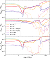 |
Fig. 1. Production rates of He II- and He I-ionizing photons (normalized to that of H-ionizing photons in the upper two panels and relative to each other in the bottom panel) as a function of the stellar-population age for different GALSEVN models. Solid orange and red lines denote GALSEVN Pop III (Z = 10−11) and extremely metal-poor Pop II (Z = 10−6), pure-binary models, while dotted lines denote the corresponding single-star models for comparison. Pop II pure-binary models for Z = 0.0001 and 0.001 are shown as dashed purple and blue lines for reference. All these models have the same zero-age Chabrier (2003) IMF. The green- and red-shaded regions indicate the areas covered by models with the three top-heavy IMFs with characteristic masses of 50 M⊙, 100 M⊙ and 200 M⊙, as described in Sect. 2.3, for Z = 10−11 and 10−6, respectively. These models are considered only up to the point where their absolute UV magnitude reaches MUV = −14, beyond which the stars are too few and the curves too noisy (see Lecroq et al. 2024, for more details). |
As the first aim of this work is to compare GALSEVN predictions with the diagnostic diagrams and Pop III (single-stars) SEDs presented by Nakajima & Maiolino (2022), we adopted nebular parameters compatible with theirs, that is,
-
ZISM = Z ∈ {10−11, 10−6, 0.0001, 0.0005, 0.001};
-
nH = 103 cm−13;
-
log⟨U⟩ = −2, given that the values considered by Nakajima & Maiolino (2022) are between −3.5 to −0.5;
-
No dust grains for the two metal-free models.
For the Pop II models with 10−6 ≤ Z ≤ 0.001, we adopted the same values of C/O = 0.17 and ξd = 0.3 as in the “standard” models of Lecroq et al. (2024) and the same abundance scaling with Z as presented in Gutkin et al. (2016).
Nakajima & Maiolino (2022) adopted a primordial He/H abundance of 0.0805, following Hsyu et al. (2020). They also considered a completely metal-free ISM4. We have tested these assumptions against Pop III models with metal abundances scaled for Z = 10−11 following the method presented by Gutkin et al. (2016) and found that the two approaches give very similar results. We therefore chose to adopt the value of Hsyu et al. (2020) for the primordial He abundance, and to turn off metals as well as dust grains in CLOUDY, for the sake of consistency in our comparison with the work of Nakajima & Maiolino (2022). This choice should have very little impact on the predictions presented in the next sections.
We also tested the impact of adopting a plane-parallel geometry, as assumed by Nakajima & Maiolino (2022), rather than a closed spherical geometry for CLOUDY calculations. The results obtained under the two assumptions being extremely similar, we chose not to investigate this aspect further.
We note that, with the assumptions presented here, the only emission-line features relevant to the metal-free models are those related to H and He. We also point out that, as our models do not follow the increase in gas-phase metallicity with stellar population evolution, strictly metal-free models should be considered only up to the time of the explosion of the first SN. This limitation will be discussed further in Sect. 3.
3. Emission properties of EoR galaxies
As Pop III stars are expected to be able to trigger intense He II-line emission (e.g., Inoue 2011; Venditti et al. 2024), we first focus on He II-related spectral features and ionizing photons. After discussing GALSEVN predictions for UV-optical line emission and SEDs, we then look into the predicted H-ionizing photon production rate and its dependence on time and metallicity. Finally, we complete the analysis of the predicted stellar populations by examining other important reionization tracers, such as the LW-band emission, which, as previously discussed, conditions the possibility of star formation in a circumstellar gas cloud, and the statistics of SNe, related to the chemical enrichment in pristine star-forming regions.
3.1. Ultraviolet and optical emission
To investigate the UV and optical emission-line properties of EoR galaxies, we begin by examining the ionizing SEDs predicted by GALSEVN for populations of single and binary Pop III stars. Since stellar effective temperature generally increases with decreasing metallicity (because the reduced opacity makes stars hotter), we expect Pop III models to have higher rates of very high-energy photons than more metal-rich ones. For massive stars at extremely low metallicities (Z ≲ 10−10), this phenomenon is amplified by the initial absence of the trace amounts of C, N and O necessary to burn H through the CNO cycle in massive stars. For these extremely low metallicity stars, the only channel for hydrogen fusion is the proton-proton (p-p) process, which is less efficient as a thermostat than the CNO cycle. Thus, gravitational contraction in the late pre-main sequence phase continues until the core reaches the high temperature and density needed to initiate the triple-alpha process (i.e., He burning), which provides the trace amounts of carbon to activate the CNO cycle. The whole structure of massive stars is therefore more compact and hotter at low metallicities (Marigo et al. 2001; Costa et al. 2023)5. Moreover, as the emission is dominated by the most massive stars at early ages, single and binary models should coincide up to ages around 1 Myr, when the most massive stars leave the main sequence.
Figure 1 shows the production rates of He II- and He I-ionizing photons, normalized to that of H-ionizing photons, as a function of the stellar-population age for different GALSEVN models. We show models of Pop III stellar populations (Z = 10−11, represented in orange) and extremely metal-poor Pop II stellar populations (Z = 10−6, in red), with solid lines for pure-binary and dashed lines for single-star models. Pop II models with Z = 0.0001 and 0.001 are represented as dotted lines (the model with Z = 0.0005, not shown for clarity, would lie between these two models). These models all have the same zero-age Chabrier (2003) IMF. As expected from the above argument, models with Z = 10−11 and 10−6 have much higher ṄHe II than models with metallicities of a few percent of solar at early ages, due to their main sequence (MS) being shifted to higher temperatures6. Figure 1 also confirms that the difference between single- and binary-star models appears after the first million years of evolution (as already highlighted in figure 1 of Lecroq et al. 2024). Then, around 2 Myr, both Pop III and Pop II binary-star models exhibit a high ṄHe II, which is absent in single-star models. This arises from the formation of pure-He, WNE-like products of massive-star stripping. However, it is interesting to note that this increase in ṄHe II is modest for Z = 10−11 and becomes more pronounced as metallicity increases. This is due to the more rapid evolution of extremely low metallicity stars, because of their accelerated and hotter central-H burning: the WNE-like products of the evolution of the most massive stars begin to produce ionizing photons before most of the lower-mass stars leave the MS. Finally, another notable difference arises at ages greater than ∼40 Myr, where the production-rate ratios of high-energy photons drops in Pop II models before rising again. This is due to the contribution from accretion disks of XRBs, which grows at earlier ages in Pop III models due to the faster stellar evolution7. This feature, consistent with the growing impact of XRB accretion disks with population age as suggested in previous studies (see Section 4.3 of Lecroq et al. 2024), occurs at ages beyond the primary focus of the present study.
These differences in behavior between Pop III and Pop II models, as well as between single and binary stars, are less marked and appear later in the case of ṄHe I. This is because the conditions to produce photons capable of singly ionizing He are less extreme – the first ionization energy of helium being 24.6 eV, less than half the 54.4 eV required to doubly ionize it.
The green- and red-shaded regions show the areas covered by models with the three top-heavy IMFs with characteristic masses of 50 M⊙, 100 M⊙ and 200 M⊙ described in Sect. 2.3, also with metallicities of Z = 10−11 and 10−6 respectively. Their evolution is shown until their absolute UV magnitude reaches MUV = −14, at which point only few stars remain, and the models become stochastically dependent on the seed used to draw their initial properties, as described by Lecroq et al. (2024, see their figure 10). The Z = 10−11 model exhibits a globally higher ṄHe II with this choice in IMF, resulting from a large fraction of extremely massive stars. This tendency is somewhat less strong for the slightly cooler Z = 10−6. Once again, the evolution of ṄHe I is very similar to that of models with a Chabrier (2003) IMF, since the difference in the fraction of very massive stars does not influence much the production rate of medium-energy ionizing photons.
We now consider the zero-metallicity stellar-population models of Schaerer (2003), based on an earlier version of the Padova evolutionary tracks for single zero-metallicity stars with negligible mass loss, complemented with other models for stars with high mass loss (Lejeune & Schaerer 2001; Meynet & Maeder 2002), both sets covering the mass range from 1 M⊙ to 500 M⊙. These stellar tracks do not include binary interactions or the effects of rotation. These models are provided for a range of modified Salpeter (1955) IMFs with different lower- and upper-mass cut-offs in the interval between 1 and 500 M⊙, as described by Raiter et al. (2010). We compare the predictions of these models with those of standard GALSEVN models with a Chabrier (2003) IMF truncated at 0.1 and 300 M⊙ for primary stars and a Sana et al. (2012) distribution of secondary-to-primary mass ratios at age zero (single stars being modeled as noninteracting binaries). Such an IMF can lead in binary-star populations to the presence of merged stars with masses up to ∼600 M⊙. For completeness, we investigated the impact of adopting an upper mass cut-off of 100 M⊙ instead of 300 M⊙. We found the effect on ṄHe II/ṄH and ṄHe I/ṄH to be limited, due to the very small fraction of stars in the upper part of Chabrier (2003) distribution, and the extremely short lifetime of these very massive stars. Moreover, low-metallicity stars with masses up to ∼300 M⊙ have been observed in local environments (e.g., Crowther et al. 2016; Smith et al. 2016, see also Vink et al. 2011), and are expected to become more frequent at lower metallicities and higher redshift. Since in any case Pop III stars are expected to be very massive (up to ∼1000 M⊙ for Pop III stars), we chose not to investigate this aspect further here and fix the upper mass cut-off of GALSEVN models at 300 M⊙ for the remainder of this discussion.
Figure 2 compares the ionizing SEDs of Schaerer (2003) Pop III models for different IMFs with the GALSEVN Z = 10−11 and 10−6 predictions presented in Fig. 1. The evolution of ṄHe II and ṄHe I is quite similar between the standard model of Schaerer (2003), which uses a Salpeter (1955) IMF truncated at 1 and 500 M⊙ (in dark purple), and the GALSEVN single-star Pop III (Z = 10−11) model (dashed orange). Slight differences in ṄHe II between 1 and 2 Myr likely stem from differences in the stellar tracks and spectral libraries used in the two models.
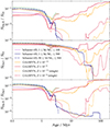 |
Fig. 2. Same as Fig. 1, but comparing the prediction of GALSEVN and Schaerer (2003) Pop III models. The solid- and dashed-orange and red curves represent the same GALSEVN Z = 10−11 and 10−6 models as in Fig. 1, with a Chabrier (2003) IMF truncated at 0.1 and 300 M⊙ for primary stars, combined with a Sana et al. (2012) distribution of secondary-to-primary mass ratios at age zero (with single stars modeled as noninteracting binaries). The green- and red-shaded regions indicate the areas covered by models with the same three top-heavy IMFs with characteristic masses of 50 M⊙, 100 M⊙ and 200 M⊙ as in Fig. 1. The solid purple, solid blue and dot-dashed blue curves show the zero-metallicity, single-star models of Schaerer (2003) for three Salpeter (1955) IMFs with different lower- and upper-mass cut-offs. |
The model by Schaerer (2003) with a Salpeter (1955) IMF truncated at 1 and 100 M⊙ exhibits a ṄHe II/ṄH ratio about five times lower than those with an IMF reaching 500 M⊙ at the earliest ages. This difference becomes less pronounced as the most massive stars leave the MS phase. In the Schaerer (2003) model with a Salpeter (1955) IMF truncated at 50 and 500 M⊙, the ṄHe II/ṄH and ṄHe I/ṄH ratios are initially slightly boosted relative to the other two models by the removal of the of the coolest ionizing stars, although they remain below the predictions of the GALSEVN models with top-heavy IMFs.
Based on these preliminary considerations regarding the Schaerer (2003) SEDs used by Nakajima & Maiolino (2022) to predict the properties of EoR galaxies, it is now interesting to compare GALSEVN predictions with the diagnostics these authors propose to differentiate ionization by Pop III stars from that by other high-energy sources in emission-line diagrams: pristine, direct-collapse black holes (DCBHs)8, evolved Pop II stars and metal-enriched AGNs. Nakajima & Maiolino (2022) considered theoretical DCBH SEDs composed of a black-body-like spectrum peaking in the ultraviolet combined a power-law tail in the X-ray range, similar to AGN emission (Valiante et al. 2018), with adjustable black-body temperature and spectral index of the power law. They also considered Pop III stars and DCBHs evolving in an enriched medium of adjustable metallicity. Nakajima & Maiolino (2022) computed the ionizing spectra of Pop II galaxies using BPASS binary-star models with metallicities ranging from 10−5 to 10−3, for 10 Myr-old stellar populations with constant SFR. They modeled the ionizing radiation from AGNs using the same templates as for DCBHs but with higher metallicities. They then used the CLOUDY photoionization code to compute the nebular emission produced by these different sources, with adjustable parameters similar to those detailed in Sect. 2.3.
In their paper, Nakajima & Maiolino (2022) investigated several emission-line diagrams able to isolate the signatures of either Pop III stellar populations or pristine DCBHs. They conclude that ionization by Pop III stars can be best discriminated based on the equivalent widths of He II λ4686 and, to a lesser extent, He II λ1640. Extreme values of these equivalent widths cannot be reproduced by any other source in their models, including primeval DCBHs. They also find the line ratios He II λ4686/Hβand He II λ1640/Lyαuseful to identify populations of Pop III stars with a top-heavy IMF, although these ratios do not discriminate between zero-metallicity stars and DCBHs. Nakajima & Maiolino (2022) also show that diagrams involving He Ilines are not good indicators of metallicity, since the values for Pop II and Pop III stellar populations are similar for these ratios. They finally identify three criteria and tendencies based on these emission lines to identify Pop III stars in emission-line diagrams (see their figures 2, 3, and 6).
We plot these emission-line diagrams and the location of the Nakajima & Maiolino (2022) models in Fig. 3, with the region corresponding to Pop III stars shown in shaded gray. Although the diagram represented in Fig. 3b) is not strictly identified as a diagnostic diagram, it is also useful as it can be used to discriminate between several values of nH. The model predictions presented by Nakajima & Maiolino (2022) for DCBHs, evolved Pop II galaxies, and AGNs – over their whole range of gas-phase metallicity, log⟨U⟩, nH, and IMFs – appear in this figure as color-shaded regions (respectively in red, blue, and green). The colored dots in Fig. 3 show the locations of zero-age9 GALSEVN SSP models with different metallicities and IMFs.
Figure 3 shows that the GALSEVN predictions for Z = 10−11 strongly support the criteria proposed by Nakajima & Maiolino (2022) to identify signatures of Pop III stellar populations. These criteria appear stringent enough that even Pop II models with Z = 10−6 fall below the identified thresholds. This agreement is not surprising, as Fig. 2 shows a similarity in the ionizing SEDs of the models, especially at early ages, where binaries are not a decisive factor. The most effective diagnostic diagram appears to be EW(He II λ4686) versus He II λ4686/Hβ, as it clearly separates regions populated by evolved galaxies, AGNs, DCBHs, and zero-metallicity models. The equivalent ultraviolet diagram of EW(He II λ1640) versus He II λ1640/Lyαalso distinguishes these sources effectively, although there is some overlap in the lowest-EW(He II λ1640) part of the gray-shaded region. In contrast, the pure line-ratio diagram of He II λ4686/Hβversus He Iλ5876/Hβseparates evolved galaxies from all other sources effectively, but struggles to differentiate AGNs and DCHBs from zero-metallicity stars. This diagram does, however, show a strong dependence on nH, as indicated by the horizontal arrows pointing to the locations of equivalent models with nH = 102 and 104 cm−3, for the lowest two metallicities. Thus, while this diagram does not fully resolve all sources, it provides useful complementary information for Pop III diagnostics.
We note that the predictions of the GALSEVN model for evolved stellar populations with Z = 0.0001, 0.0005, and 0.001 are also in good agreement with those of Nakajima & Maiolino (2022). This is not surprising, given the agreement between GALSEVN and BPASS predictions at early ages (see figure 4 of Lecroq et al. 2024).
We did not investigate predictions for Pop III stars evolving in a slightly enriched ISM, as do some of the models presented by Nakajima & Maiolino (2022). Although our approach would allow such modeling (see section 3.3.3 of Lecroq et al. 2024), we made this choice because of the short lifetimes of these stars, and because we focus in this study on the very first generations of Pop III stars.
It is of interest to examine the predicted signatures of primeval sources not only at zero age, but also in their evolution with time, to be able to estimate the probability of observing them in the areas of diagnostic diagrams identified above. We therefore also discuss the time evolution of these spectral features for the GALSEVN models commented above. Again, the GALSEVN models presented here do not take into account the enrichment of the surrounding medium through stellar evolution, but assume a constant gas-phase metallicity equal to that of the ionizing stars. Such enrichment could considerably alter the values of ZISMfor the lowest metallicities, which would be highly sensitive to the presence of even trace amounts of metals. We therefore stopped our calculations at the time when the first SN appeared for each population, to ensure that the surrounding medium would not have yet been polluted by new metals.
Figure 4 shows the time evolution of the same GALSEVN SSP models as displayed at zero age in Fig. 3. For clarity, the evolution has been detailed only for models with a Chabrier (2003) IMF, the areas sampled by models with top-heavy IMFs appearing as green- and red-shaded regions for the metallicities Z = 10−11 and 10−6, respectively (while regions identified by Nakajima & Maiolino 2022 as populated by primeval DCBHs, Pop II galaxies, and AGNs have been omitted). In each model, an orange star marks the time of appearance of the first SN, when the model is stopped, corresponding to about 2.3 Myr for all models. Fig. 4 reveals that the evolution of all considered spectral features is very rapid at these early ages. Indeed, models with Z = 10−11 remain within the gray zones identified above to select ionization by Pop III stars only for ages up to ∼1 Myr. This makes the probability of observing Pop III stars in this state quite low. Models with higher metallicities exhibit loops toward stronger He II λ1640 spectral features, around 1 Myr and later after 2 Myr. These loops, especially visible for the He II λ1640 equivalent widths predicted for Z = 10−6, are due to the sudden increase in the production rate of He II-ionizing photons already discussed in Fig. 1. However, the implied increases in EW(He II λ1640), EW(He II λ4686), and He II λ4686/Hβare not intense enough to bring these models over the thresholds of the Pop III diagnostic criteria.
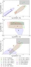 |
Fig. 3. Diagnostic diagrams proposed by Nakajima & Maiolino (2022) to differentiate ionization by Pop III stars from that by other high-energy sources. The markers represent zero-age, pure binary-star GALSEVN models with different metallicities and IMFs, color-coded as indicated on the bottom. The gray-shaded area denotes the region identified by Nakajima & Maiolino (2022) as populated by Pop III stars, while the other colored regions correspond to areas populated by primeval DCBHs, evolved (Pop II) galaxies, and AGNs, as indicated. In panel (b), the horizontal arrows for Z = 10−11 and 10−6 indicate the positions of corresponding models with nH = 102 cm−3 (left-pointing) and 104 cm−3 (right-pointing). |
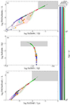 |
Fig. 4. Same diagnostic diagrams as in Fig. 3. As before, the gray-shaded zone in each diagram indicates the location of models powered by Pop III stars, as identified by Nakajima & Maiolino (2022). The different curves with dots show the temporal evolution of the GALSEVN SSP models presented at zero age in Fig. 3, with age referenced by the color bars on the right. For each curve, an orange star marks the appearance of the first SN, at which point the model is stopped in the present study. The red- and green-shaded regions show the areas covered by models with top-heavy IMFs, as in Figs. 1 and 2. Figures 3 and 4 overall highlight the fact that the GALSEVN models support the criteria presented by Nakajima & Maiolino (2022) to identify ionization by Pop III stellar populations. The figures also confirm that these criteria as strict enough to efficiently separate Pop III signatures from those from other possible sources of high-energy photons. However, the high thresholds of these criteria make them accurate for only a very short time, making the probability of actually observing stellar populations in this regime very low. |
3.2. Production efficiency of ionizing photons
A crucial parameter to constrain the amount of H-ionizing photons available for reionization in simulations is the Lyman-continuum escape fraction, fesc, defined as the fraction of all ionizing photons produced that can escape through the ISM and IGM to ionize intergalactic neutral hydrogen. Recently, significant efforts have been made to directly measure fesc at redshifts up to z ∼ 4. However, because of the substantial increase in IGM opacity at higher redshift (e.g., Inoue et al. 2014), fesc in the EoR can be inferred only indirectly and through model-dependent approaches. To address this limitation, indicators need to be established based on local observations, which can link readily measurable quantities, such as line emission (which traces the fraction of ionizing photons absorbed by the gas) and nonionizing UV luminosity. When combined with the production efficiency of ionizing photons, ξion, which links the production rate of H-ionizing photons to that of nonionizing ultraviolet photons, such observations may provide more confident estimates of fesc at high redshift.
Three different definitions of the production efficiency of ionizing photons can be found in the literature, each with varying degrees of appropriateness depending on whether the focus is on a theoretical or observational study:
-
The stellar ionizing-photon production efficiency,
 (3)
(3)where
 is the intrinsic stellar monochromatic ultraviolet luminosity, that is, the UV luminosity that would be observed in the absence of gas and dust in the galaxy;
 -
The stellar+nebular ionizing-photon production efficiency,
 (4)
(4)where LHII is the UV luminosity accounting for the effects of dust absorption within H II regions and nebular recombination-continuum emission;
-
and the observed ionizing-photon production efficiency,
 (5)
(5)where LUV is the observed, uncorrected UV luminosity.
These monochromatic UV luminosities are computed from the stellar spectrum, the stellar+nebular transmitted spectrum, and the rest-frame observed spectrum, respectively, by averaging the emission over a 100 Å-wide window centered on 1500 Å (see, e.g., Robertson et al. 2013).
To circumvent the difficulty posed by uncertainties over fesc values as explained above, we focused more particularly on two limiting cases, studying both the stellar coefficient  – which corresponds to the case where fesc = 1, meaning that all ionizing photons escape from the surrounding H II region – and the nebular coefficient
  – corresponding to fesc = 0, as we are considering an ionization-bounded H II region. The former depends only on stellar-population properties, that is, mainly age, metallicity, and IMF. Simulations often consider a fixed value of
  , constant with age and chemical evolution. One of the goals of the present work is to provide an overview of
  and
and  for GALSEVN SEDs, including how they evolve with these stellar-population parameters, which we can achieve self-consistently with the ultraviolet and optical spectral signatures mentioned above.
The nebular ionizing-photon production efficiency  is a more direct observable than
  , as it can be constrained by observations corrected for dust attenuation outside the ionized region. We therefore begin our analysis by looking at the evolution of
  with time and metallicity, for the SSP models discussed in the previous section. The quantity
  was calculated using the rate of H-ionizing photons predicted by the GALSEVN stellar-population models, and the UV luminosity computed from the spectrum output by CLOUDY, to account for the recombination continuum and dust absorption inside the ionized region.
Figure 5 shows the time evolution of  for the same GALSEVN binary SSP models as in Fig. 1. The time of appearance of the first SN in the lowest metallicity populations is marked by the vertical dashed line, to indicate the beginning of chemical enrichment. Estimates of ξion have flourished in recent work, both from simulations and from observational constraints. Analytical reionization models often assume a canonical value in the range
  –25.3 (e.g., Robertson et al. 2013), shown by the gray-shaded region in Fig. 5. We can also compare GALSEVN predictions to the ξion ranges estimated in two recent observational studies. Bouwens et al. (2016) derived their values from observations of star-forming galaxies in the GOODS field, at redshifts z ∼ 3.8–5.4, based on the measured UV-continuum slope and Hαintensities. Chevallard et al. (2018) obtained their values by fitting the SEDs of ten nearby analogs of primeval galaxies from HST/COS observations, using the BEAGLEspectral-interpretation tool. The ranges of ξion values in these two studies appear as green- and blue-shaded regions on Fig. 5. These results are in general agreement with those derived in several other recent works, which used different methods to retrieve the values of
  and
and  from observations at various redshifts (0.3 ≲ z ≲ 9), and whose ranges of values have not been plotted in Fig. 5 for the sake of clarity (e.g., Stark et al. 2015; Schaerer et al. 2016; Izotov et al. 2017; Matthee et al. 2017; Stark et al. 2017; Shivaei et al. 2018, see section 5 of Chevallard et al. 2018 for a more detailed comparison).
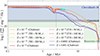 |
Fig. 5. Nebular ionizing-photon production efficiency |


Figure 5 shows that the GALSEVN predictions are very similar for all metallicities at early ages, with a relatively high estimated  (still falling within the observed range), which remains almost constant at first, while most stars evolve on the MS. After ∼1 Myr, the dependence of the evolution becomes more pronounced. The lowest-metallicity models generally keep a higher
  , and the decrease in
  seems to be almost linear with slopes depending on metallicity until ∼30 Myr. The slope seems to steepen with increasing metallicity. This is expected, due to the higher ionizing power of stars with extremely low metallicity, resulting from their specific properties (e.g., evolutionary tracks shifted toward higher temperatures), as discussed in the previous section.
Moreover, comparison of the models with a Chabrier (2003) and top-heavy IMFs reveals that the IMF does not appear to be a crucial parameter for the predicted  values. While the predicted values for top-heavy IMFs are slightly higher at early ages, the main difference is a pronounced feature just before 2 Myr, when most massive stars reach the end of their H-burning phase, resulting in a drop in the production of ionizing photons until the appearance of hot, WNE-like products of binary evolution. As before, we stop the evolution of models with top-heavy IMFs when their absolute UV magnitude reaches MUV = −14.
Figure 5 shows overall good agreement between GALSEVN predictions for  and recent observations. It also reveals a dependence of
  on time and metallicity, which is almost negligible for approximately the first million years, before becoming more pronounced.
According to simulations of early galaxy formation (e.g., Finkelstein et al. 2019) and recent observational constraints on the nonionizing UV luminosity density (e.g., Atek et al. 2024), with such high values of  , the escape of only a few percent of ionizing photons from nascent galaxies would suffice to reionize the Universe. The fact that such high values of
  are naturally produced by GALSEVN models for metallicities up to a few percent of solar supports the major role that early star-forming galaxies are likely to have played as reionization drivers.
For some applications to the modeling of early galaxy formation, it may be useful to have a simple analytical expression for estimates of  as a function of the time and metallicity. We derive such relations here for models with a Chabrier (2003) IMF (as Fig. 5 shows, models with top-heavy IMFs have similar properties at early ages).
The general shape of the curves in Fig. 5 suggests a fit with two linear regimes, before and after the breaks that occur between 1 and 2 Myr, depending on the metallicity. As the two extreme metallicities, Z = 10−11 and 0.001, appear to bracket the intermediate ones, and as the slope after the break appears to decrease monotonically with metallicity, we present fits only for these two metallicities, assuming that the relations for the intermediate metallicities can then be interpolated. We find that
 (6)
(6)
and
 (7)
(7)
provide reasonable approximations to the actual models for Z = 10−11 and Z = 0.001 respectively, as illustrated by Fig. 6.
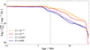 |
Fig. 6. Bimodal linear fits adopted to represent |

It is also of interest to provide a means of estimating the stellar ionizing-photon production rate  , which is often used (in combination with the fesc parameter) in simulations of the reionization epoch. We can achieve this by combining the above expressions for
  with an estimate of the ratio between
  and
and  . For simplicity, we focused on the initial, bright phase with nearly constant
  at ages below 1 Myr (Fig. 5), during which massive stars evolve on the main sequence. Fig. 7 shows the evolution of the
  /
/ ratio during this phase, for the different metallicities, for the same GALSEVN binary SSP models with a Chabrier (2003) IMF as in Fig. 1. The ratio is almost constant during this phase and decreases with increasing metallicity, reflecting the associated increasing absorption of stellar UV luminosity by dust in the H II region (at fixed dust-to-metal mass ratio ξd). We computed the time-averaged value of this ratio for each metallicity (shown as a red horizontal line in each panel), which we report in Fig. 8 with uncertainties reflecting the offset of the most extreme value from the time-averaged ratio. The dependence of this time-averaged value on metallicity can be well approximated by the relation
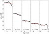 |
Fig. 7. Time evolution of the |


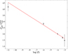 |
Fig. 8. Illustration of the fit to time-average values of |


 (8)
(8)
obtained using weights inversely proportional to the uncertainties and shown as the red line in Fig. 8.
3.3. Other properties
In this subsection, we present complementary quantities predicted by our GALSEVN models of EoR galaxies, which may offer additional probes of the stellar physics at play in the early Universe. These include the production rate of Lyman-Werner photons and the rates of different types of SNe, which can provide important information about chemical enrichment.
3.3.1. Lyman-Werner photon production rate
Unlike most high-energy photons, which are rapidly absorbed by neutral H in the IGM, LW photons have a very long mean free path due to their relatively low energies, just above the Lyman limit. It is therefore important to account for LW photons self-consistently in simulations studying the formation of the first cosmological structures, as this has strong implications for star formation, and hence, for stellar properties, feedback, chemical-enrichment timescales, etc., as explored in recent studies by Gessey-Jones et al. (2022) and Incatasciato et al. (2023).
Incatasciato et al. (2023) present an in-depth study of the LW radiation field, its evolution with redshift and its consequences on H2 photo-dissociation and star formation. They used SPS models to predict LW-photons emission for both Pop III and Pop II stellar populations. Their calculations were based on the Schaerer (2002) models with different IMFs for Z = 0, and on BPASS models with different IMFs for Pop II (Z = 0.0005) populations. Incatasciato et al. (2023) conclude that the mean LW intensity must have increased significantly from z ∼ 23 to z ∼ 6 – primarily due to massive star-forming galaxies – and highlight the importance of incorporating LW radiation into cosmological simulations for a realistic understanding of early galaxy formation. They examine the complexities of modeling the LW background radiation, comparing various models and noting the impacts of differing assumptions on the predictions. They also investigate the evolving minimum halo mass required for Pop III star formation under LW influence, advocating the high sensitivity of such predictions to model limitations. This, and the support by recent JWST observations of actively star-forming galaxies at high redshifts, indicates the crucial role of LW radiation in star formation within low-mass halos in the early Universe.
In Fig. 9, we compare the fiducial model of Incatasciato et al. (2023, available for ages greater than 1 Myr) for populations of Pop II stars (using Z = 0.0005 BPASS models with the Chabrier 2003 IMF) and Pop III stars (using zero-metallicity models from Raiter et al. 2010 with a lognormal IMF over 1–500 M⊙) with predictions from the GALSEVN model. All production rates are normalized to a total initial stellar mass of 1 M⊙. The production rates of LW photons computed by Incatasciato et al. (2023) are in general agreement with those obtained with the GALSEVN model for a Chabrier (2003) IMF. The main difference arises before ∼3 Myr: in the Incatasciato et al. (2023) model, Pop III stars initially produce more LW photons than their Pop II counterparts, before this trend reverses over time. In contrast, the GALSEVN model predicts that Pop II stellar populations consistently produce more LW photons than Pop III ones at all times. The GALSEVN model also reveals a general trend of increasing  with metallicity at all ages, driven by the gradual shift of the peak wavelength of the hot, near-black-body spectra of the most massive stars on the upper main sequence, from the far-UV to the near-UV. Models with top-heavy IMFs initially exhibit much higher LW photon-production rates (per unit stellar mass), before declining much more steeply shortly after 1 Myr as the most massive stars die out. This behavior is also observed in the Incatasciato et al. (2023) models, as represented in their figure 2.
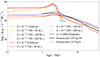 |
Fig. 9. Lyman-Werner photon-production rate (in the wavelength range 912 Å–1150 Å) as a function of the stellar-population age for the same GALSEVN models as in Fig. 1 (normalized to a total initial stellar mass of 1 M⊙ integrated over 0.1–300 M⊙). The models with Z = 0.0001 and 0.001, which are nearly indistinguishable from the Z = 0.0005, are omitted here for clarity. For reference, the predictions of Incatasciato et al. (2023) for populations of Pop II stars (using Z = 0.0005 BPASS models with the Chabrier 2003 IMF) and Pop III stars (using zero-metallicity models from Raiter et al. 2010 with a lognormal IMF over 1–500 M⊙) are shown as dotted and solid black curves, respectively. |
We find LW photons-production rates in general agreement with those reported by Incatasciato et al. (2023), supporting their conclusions on the importance of including LW radiation in simulations of early galaxy formation and its influence on star formation in low-mass halos. Given the LW photon-production rates predicted here, it is likely that, after the first generations of stars have evolved, most of the molecular H2 in the ISM has been photo-dissociated. At this stage, however, star-forming halos are expected to have reached virial temperatures high enough for atomic cooling to take over, ensuring that star formation continues (e.g., Oh & Haiman 2002), until metallicity rises enough for metals to become the most efficient coolants.
3.3.2. Supernova rates
The study of the different types of SNe occurring in a stellar population provides useful information about the evolutionary paths followed by individual stars. The physical conditions reached during the final core collapse of a star, which are primarily determined by its mass and composition, allow for the differentiation between different types of explosive phenomena.
Type-Ia SNe arise at the surface of accreting white dwarfs, when their mass exceeds the Chandrasekhar limit for white dwarf stability (∼1.4 M⊙). These events exhibit characteristic energies on the order of 1051 erg, and release relativistic ejecta composed mainly of iron-peak elements due to the runaway fusion reactions in the exploding white dwarf. As indicators of the proportion of low-mass stars in binary systems, type-Ia SNe are also the primary contributors to Fe enrichment in the ISM. On the other hand, type-II SNe are the product of the evolution of massive stars and are responsible for enriching the ISM in α elements (O, Ne, Mg, Si, S, Ca). Pair-instability SNe (PISNe) are particularly interesting as indicators of mass distributions in a stellar population, as they arise only from extremely massive stars, with zero-age MS masses between typically 130 and 250 M⊙10. PISNe release enough energy to completely disrupt the stellar remnant, creating a mass gap in the mass spectrum of black holes (Spera et al. 2015; Belczynski et al. 2016; Woosley 2017; Spera & Mapelli 2017). Thus, studying PISNe in a stellar population provides insight into how many objects are expected to populate this mass gap. Stars slightly less massive than PISN progenitors, with zero-age MS masses typically between 60 and 130 M⊙, can still reach He-core masses large enough to convert photons into electron-positron pairs. However, in these cases, the subsequent pair annihilation leads to core contraction and explosive burning of oxygen and silicon, but not enough energy is generated for a complete disruption. Instead, these stars undergo Pulsational PISNe (PPISNe), experiencing multiple pulsations which release significant kinetic energy through mass loss before eventually collapsing into a compact remnant (typically a black hole).
Due to the very high masses of their progenitors and their correspondingly short lifetimes, PISNe and PPISNe are expected to arise only at early ages. Instead, because of the longer evolutionary timescales of low-mass stars and white dwarfs, type-Ia SNe are expected to occur after several tens of millions years. This stark difference in timescales makes the α-to-Fe element ratio in the ISM an excellent indicator of the age of a stellar population.
Figure 10 shows the time evolution of the different types of SNe arising in the same binary-star GALSEVN SSP models as in Fig. 1. We ignore nonexploding, ‘failed’ SNe leading to the formation of black holes (Spera et al. 2015; Spera & Mapelli 2017). For clarity, only models with a Chabrier (2003) IMF are represented (predictions for top-heavy IMFs can be inferred from these models using mass-distribution arguments). The five different metallicities are represented in different colors, while different line styles represent the different types of SNe.
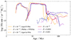 |
Fig. 10. Supernova rate as a function of the stellar-population age for the same binary-star GALSEVN models with a Chabrier (2003) IMF as in Fig. 1 (normalized to a total initial stellar mass of 1 M⊙integrated over 0.1–300 M⊙). Different metallicities are shown in different colors, and different types of SNe are distinguished by line styles (short-dashed for pair-instability, solid for “classical” type-II, and dot-dashed for type-Ia SNe). |
As expected, the PISNe+PPISNe peak in Fig. 10 arises between 2 and 6 Myr across all metallicities. This rate is not strongly affected by metallicity, as the metallicities represented here are all fairly low. For higher metallicities, this rate would decrease, eventually falling to zero for metallicities above Z = 0.01 for PISNe and 0.018 for PPISNe (Spera & Mapelli 2017). Other types of type-II SNe, from lower-mass progenitors, emerge around 10 Myr and persist for a few tens of Myr. The onset and duration of this peak are similar for all metallicities, which is not surprising as the IMF is the same for all models. Yet, the duration of the peak appears slightly shorter at the lowest metallicity, likely due to the faster evolution of the hotter stars at such low metallicity. Type-Ia SNe first appear around 30 Myr, displaying a similar behavior across all metallicities.
Finally, we note that chemical enrichment in Pop III models begins around 2 Myr, marked by the appearance of the first PISNe.
4. Gravitational-wave signal from Pop III binary black holes
As previously mentioned, direct optical observations of Pop III stars are extremely difficult. It is therefore useful to focus on indirect observations and multimessenger emission, as these could provide valuable counterparts to the detection of Pop III stars at high redshift. Pair-instability and core-collapse SNe, which are expected to reach luminosities of up to 1012 L⊙ (Whalen et al. 2013a,b), offer attractive opportunities for indirect detection up to z ∼ 15 (Whalen et al. 2013a,b, 2014; Smidt et al. 2014, 2015) and can trigger gamma-ray bursts (Wang et al. 2012; Burlon et al. 2016) potentially detectable up to z ∼ 20 with near-future facilities (Amati et al. 2018). However, the short duration of such transients makes their detection probability still rather low. Pop III stars can also be detected indirectly through the impact of their intense radiation on the timing and depth of the cosmological 21-cm signal. This can be explored via the incorporation of spectral models such as GALSEVN into simulations of the global 21-cm emission (e.g., Mirocha et al. 2018; Mebane et al. 2020; Gessey-Jones et al. 2022; Ventura et al. 2023; Pochinda et al. 2024). In this section, we focus on another promising indirect probe of the properties of Pop III stellar populations: binary black holes (BBHs), and in particular their mergers, which should produce potentially detectable gravitational-wave signatures – conveniently exempt from foreground contamination and line-of-sight absorption, unlike electromagnetic messengers. In this section, we adopted the most recent Planck values (Planck Collaboration VI 2020) for all cosmological parameters11.
For the sake of brevity, we do not go into detail about the basics of GW emission by two merging compact objects. We refer the reader to, for example, Maggiore (2007, 2018) for thorough reviews on GWs and more details about the gravitational signal emitted by merging BBHs.
4.1. Binary black-hole mergers in GALSEVN models of EoR galaxies
We followed pure-binary SSPs with a Chabrier (2003) IMF for the five metallicities considered in the previous sections. For each BBH system formed, we estimated the merger time based on the BH masses, separation (semi-major axis), and eccentricity at the time of formation, according to the following equation, which provides high accuracy (relative error of less than 0.6%) across the full range of eccentricities (Iorio et al. 2023):
 (9)
(9)
with
![Mathematical equation: $$ \begin{aligned} f_{\mathrm{corr} }(e) = e^2 \left[ -0.443 + 0.580(1 - e^{3.074})^{1.105 - 0.807 e + 0.193 e^2} \right] \end{aligned} $$](/articles/aa/full_html/2025/03/aa52463-24/aa52463-24-eq51.gif) (10)
(10)
(see appendix D of Iorio et al. 2023 for details).
The expected cumulative number of merging BBHs in the GALSEVN models is shown as a function of the redshift in Fig. 11. For the Pop III model, approximately a third of the total BBH population merges between z = 10 and z = 0 and contributes to this plot. The number of merging BBHs increases significantly with decreasing metallicity. This results from the less efficient mass loss at such low metallicities, which allows stars to retain more mass, making them larger and less compact, increasing the likelihood of interactions, such as mass-transfer or common-envelope phases, and leading to tighter BBHs able to merge within a Hubble time (e.g., Iorio et al. 2023). The number of mergers initially rises rapidly at high redshift, particularly in the most metal-poor models. This is due to the most massive and tightest binaries very rapidly becoming close BBHs and merging, all within a few Myr. Finally, although the total number of merging BBHs is largest for Z = 10−11, it is below that for Z = 10−6 during the first Myr. This arises from the larger masses of progenitor stars at Z = 10−11, which increase the probability of unstable mass transfer resulting in premature mergers and common envelope configurations, hence reducing the formation of very tight BBHs. The surviving, looser BBHs exhibit longer delay times before merging.
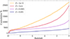 |
Fig. 11. Cumulative number of binary black hole mergers as a function of the redshift in GALSEVN populations of pure-binary stars (of 1 million pairs each) for different metallicities. |
We now focus on the masses of BBHs that merge before z = 0 according to Fig. 11. We show this distribution for black holes forming from the primary (m1) and secondary (m2) stars in Fig. 12, for the metallicities Z = 10−11, Z = 10−6, Z = 0.0001, and Z = 0.001.
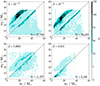 |
Fig. 12. Two-dimensional histograms of the masses of black holes in merging BBH systems, for the same GALSEVN models as in Fig. 11, for the metallicities Z = 10−11, Z = 10−6, Z = 0.0001, and Z = 0.001 (in different panels, as indicated). The quantity m1 refers to the mass of the BH formed from the primary star, whereas m2 refers to that of the BH formed from the secondary star. The total number of BBH mergers in the modeled stellar population is indicated in the lower-right corner of each panel. The identity relation is shown as a dashed line. |
Figure 12 exhibits two notable features: in each panel, the objects tend to be distributed primarily either along the identity relation, or in the upper-left corner of the diagram. This second, increasingly prominent sequence toward low metallicities, reveals that in systems where the black-hole masses are not similar, the remnant of the secondary star tends to be the most massive. This is primarily due to the inclusion of quasi-homogeneous evolution in the binary-star models, which results in compact, pure-helium secondary stars immediately after the main sequence following Roche-lobe mass transfer from the primary star. These helium stars lead to the formation of more massive black holes, almost as massive as the pure helium stars, than in models without QHE. To illustrate this, we show in Fig. 13 the analog of Fig. 12, but for binary-star models not including QHE. The sequence of BBHs with m2 > m1 is largely absent from these diagrams. At the lowest metallicities, the significantly smaller number of merging BBHs in models without QHE is mainly due to premature mergers before the secondary can form a black hole, and partly to greater mass loss from less compact secondaries, giving rise to neutron stars rather than black holes in SNe. At the highest metallicities, instead, the significantly larger number of BBHs merging by z = 0 in models without QHE results from more efficient mass loss leading to less massive secondaries and tighter systems. Hence, the inclusion of QHE in binary-star models can strongly influence the population of early BBHs that are expected to merge within a Hubble time.
4.2. Detectability of binary black-hole mergers from EoR galaxies
Having highlighted the variety in orbital and mass parameters of BBHs expected to merge between z = 10 and now in the GALSEVN models, it is interesting to investigate what fraction of mergers from Pop III precursors could actually be observed by current or near-future GW detectors. We provide in this section an estimate of the percentage of sources from the GALSEVN populations whose signal-to-noise ratio would be sufficiently high to be detected with the upcoming LIGO-Virgo-KAGRA O5 run and with the Einstein Telescope.
For the Einstein Telescope (ET), we assumed the ET-D configuration, composed of three nested triangular detectors with arms of 10 km each (e.g., Hild et al. 2008; Maggiore et al. 2020; Branchesi et al. 2023). For simplicity, we assumed the three detectors to be identical and independent. Furthermore, for simplicity, and given their sensitivities and optimal frequency ranges for detecting merging black holes with masses around 30 M⊙, we focused on these two experiments only, considering the O5 run for LIGO-Virgo and the predicted specifications for ET (expected first light in 2036, Branchesi et al. 2023). We used sensitivity curves from recent publications (Abbott et al. 2020; Maggiore 2018).
For this study, we considered the population of BBHs emerging from a stellar population formed during a single burst at z = 10, which would merge before z = 0 (using Eq. (9), as in the previous section, for this selection). We made the conventional assumption that a merger would be detectable if it gives a signal-to-noise ratio (S/N) greater than 9 for a given detector. We estimated the S/N of an individual signal following the approach outlined by Santoliquido et al. (2023), taking care of combining all three detectors of ET in the S/N calculation.
For each merging BBH, we evaluated the S/N based on the following equation12:
 (11)
(11)
where Sn(f) represents the detector sensitivity curve. The amplitude of the GW in the frequency domain,  , was computed using the PYCBC library. In line with several recent studies (e.g., Dominik et al. 2015; Taylor & Gerosa 2018; Bouffanais et al. 2019; Chen et al. 2021; Santoliquido et al. 2023), we adopted the phenomenological waveform IMRPHENOMXAS (García-Quirós et al. 2020) for compact binary mergers.
To account for the impact of the position of the objects in the sky, we randomly drew the position of each merger, considering isotropically distributed sources. We also randomly sampled the inclination angle ι of each system. More details on the exact formulæ implemented in this method, in particular for the different wave polarizations, can be found in section 2.5 of Santoliquido et al. (2023). To avoid any bias resulting from the stochastic sampling of these angles over a relatively small number of sources, we computed the number of detectable sources a hundred times for each population, from which we derive a mean value and standard deviation.
For the Pop III (Z = 10−11) and extremely metal-poor Pop II (Z = 10−6) models, corresponding to Z = 10−11 and Z = 10−6, we obtained very similar results. We found that LIGO-Virgo O5 should be able to detect at most a few percent of the sources in the simulated populations – more precisely, 6.7 ± 1.9% for Z = 10−11, and 10.2 ± 2.0% for Z = 10−6. The BBH mergers that could be detected by the LVK detectors during O5 occur at low redshift (z ≲ 1), and involve mainly systems with BH masses greater than 20 M⊙. This is in line with the larger fraction of merging BBHs at low redshift shown in Fig. 11 for Z = 10−6, compared to Z = 10−11.
On the other hand, ET-D is predicted to be able to detect 90.2 ± 4.3% of the merging BBHs for Z = 10−11, and 90.2 ± 4.0% for Z = 10−6. This finding supports the importance of studying the demographics of such predictions, as a substantial amount of observational gravitational-wave constraints may soon be available to put these predictions to the test (e.g., Santoliquido et al. 2024). However, even if most of these objects become detectable in the near future, it will likely remain challenging to conclusively identify detections as signatures of Pop III stars.
5. Summary and conclusions
In this work, we have used the GALSEVN model, introduced and discussed in detail by Lecroq et al. (2024), to compute the emission properties of extremely metal-poor stellar populations with Z = 10−11 and Z = 10−6. We compared these to GALSEVN models of metal-poor populations with higher metallicities (Z = 0.0001, 0.0005, and 0.001), and to the predictions of Nakajima & Maiolino (2022). Our results confirm that the emission-line diagnostics highlighted by Nakajima & Maiolino (2022) are effective for identifying ionization driven by zero-age Pop III stars, with the GALSEVN models providing additional information that these criteria can isolate Pop III stellar populations at ages ≲1 Myr, as shown by Figs. 3 and 4. We also provided predictions for the production efficiency of ionizing photons by these metal-poor stellar population, useful to investigate their potential role in the reionization of the Universe. To facilitate such analyses, we derived simple analytical expressions linking this efficiency directly to age and metallicity. Furthemore, we presented predictions for the production rate of Lyman-Werner photons, essential to understand the mechanisms of pristine-gas cooling and early star formation, as well as for supernova rates, which provide insight into the timescales of chemical enrichment. Finally, we explored the properties of binary black holes in these GALSEVN models, including their merger probabilities and the likelihood of detecting these events through gravitational waves. Such detections could serve as critical observational counterparts to the challenging task of directly identifying Pop III stars.
The main conclusions of this study can be summarized as follows.
-
We confirm that the ultraviolet and optical H and He emission-line diagnostics introduced by Nakajima & Maiolino (2022) (Fig. 3) are effective to discriminate between ionization by very young (≲ 1 Myr) Pop III stellar populations and other primordial or later sources (Fig. 4). We also confirm, as already shown in previous studies (e.g., Eldridge & Stanway 2012; Lecroq et al. 2024), that the production of ionizing photons beyond the first million years is dominated by processes originating from binary interactions (Figs. 1–2).
-
We find that GALSEVN models of Pop III and metal-poor Pop II stellar populations predict high production efficiencies of ionizing photons. Specifically, we find elevated values of
 relative to standard predictions, consistent with recent observational studies of galaxies in a wide range of redshifts (Fig. 5). We also provide analytical expressions to describe the evolution of
  as a function of the age and metallicity, and to relate
  with
with  , the latter being commonly used in simulations (Figs. 6–8). Comparison of our predictions with recent theoretical and observational results suggests that the escape of only a few percent of ionizing photons from nascent galaxies with such properties would be sufficient to reionize the primordial Universe.
 -
We find production rates of Lyman-Werner photon in agreement with recent simulations (e.g., Incatasciato et al. 2023), highlighting the critical role of these photons in the mechanisms and timescales of early star formation (Fig. 9).
-
Our analysis of pair-instability, type-II, and type-Ia supernova rates reveals relatively consistent behavior across metallicities ranging from 10−11 to 0.001. This analysis allows us to identify the onset of chemical enrichment in GALSEVN Pop III stellar populations at approximately 2 Myr.
-
By examining the properties of binary black holes originating from GALSEVN Pop III stellar populations, we find that the predicted merger rates and mass distributions of these systems depend critically on the inclusion of quasi-homogeneous evolution in the models. Our results suggest that most BBH mergers from such Pop III stellar populations, even at high redshifts, should be detectable with the Einstein Telescope. This high detectability positions BBH mergers as an important complement to direct observations in characterizing Pop III stellar populations in the EoR.
The Pop III stellar metallicity Z = 10−11 quoted in this work refers to the mass fraction of all elements heavier than lithium in the stellar-evolution calculations of Costa et al. (2023). The actual stellar metallicity of these models, including primordial Li, is Z ≈ 2.7 × 10⁻⁹ (Costa et al. 2025). The value Z = 10−11 was selected because the features specific to Pop III star evolution (such as the critical role of the triple-alpha reaction to activate the CNO cycle; see Sect. 3.1) appear at Z ≤ 10−10 (e.g., Cassisi & Castellani 1993; Marigo et al. 2001). For Pop II stars, the quoted metallicities (10−6 ≤ Z ≤ 10−3) refer in the standard way to the mass fraction of all elements heavier than helium.
https://gitlab.com/sevncodes/sevn. The SEVN version used in this work is the release Iorio22 (https://gitlab.com/sevncodes/sevn/-/releases/iorio22).
A star with metallicity lower than 0.004 can be spun up by the accretion of substantial material through stable Roche-lobe overflow mass transfer, leading to the replenishment of its core with fresh hydrogen via rotational mixing. The star remains fully mixed until it burns all its hydrogen into helium (ending as a pure-He star) at nearly constant radius. During this QHE phase, it brightens and its temperature increases, thereby augmenting the population of compact, hot luminous stars.
CLOUDY offers a “no metals” option, as well as a “no dust grains” option.
In contrast, since low-mass stars are well-supported by the p-p cycle alone, their structure is affected only through the impact of metallicity on opacity.
While the MS of Z ≳ 0.0001 models roughly spans from 20,000 to 60 000 K, it is shifted to the 40 000–80 000 K range for Z = 10−6 and 45 000–100 000 K for Z = 10−11.
Pop III models not including the emission from XRB accretion disks do not exhibit this feature. Instead, they show energetic-photon production rates which fall off more rapidly than in Pop II models, due to their faster evolution and their lack of WNE-type stars, present at late ages in Pop II models.
DCHBs are black holes with masses between 105 and 106 M⊙, which might have formed directly from the collapse of pristine gas clouds in the early Universe (see, e.g., Volonteri 2012; Valiante et al. 2016; Beckmann et al. 2019; Inayoshi et al. 2020, for reference).
In the Nakajima & Maiolino (2022) models, all stars begin their evolution on the zero-age main sequence. Instead, in the GALSEVN model, which includes pre-MS evolution, SSPs ignite when the most massive stars approach the MS. This difference in timing is minimal, as pre-MS evolution lasts only about 1% of the MS duration, and does not impact the conclusions of this paper.
The exact range depends on metallicity, which controls the efficiency of stellar winds and their influence on reaching the He-core mass required to form electron-positron pairs and trigger the PISN mechanism (see, e.g., fig. 2 of Spera & Mapelli 2017).
Specifically, we used the matter and dark-energy density parameters Ωm = 0.315 and ΩΛ = 0.6847, and the Hubble constant H0 = 67.4 km s−1 Mpc−1.
This equation corresponds to the frequency treatment applied in the matched filtering technique, which allows on-the-fly detection of GWs from continuous observations (see, e.g., Dal Canton et al. 2014, for more details).
Acknowledgments
We thank the referee for useful comments. We are grateful to D. Schaerer and K. Nakajima for sharing electronic versions of their models and to M. Dall’Amico for helpful discussions. G.I. acknowledges financial support under the National Recovery and Resilience Plan (NRRP), Mission 4, Component 2, Investment 1.4, - Call for tender No. 3138 of 18/12/2021 of Italian Ministry of University and Research funded by the European Union – NextGenerationEU. F.S. acknowledges financial support from the AHEAD2020 project (grant agreement n. 871158). M.M. acknowledges financial support from the German Excellence Strategy via the Heidelberg Cluster of Excellence (EXC 2181 - 390900948) STRUCTURES. M.M., F.S., G.C., and G.I. also acknowledge financial support from the European Research Council for the ERC Consolidator grant DEMOBLACK, under contract No. 770017 (PI: Mapelli). G.B. acknowledges financial support from the National Autonomous University of México (UNAM) through grants DGAPA/PAPIIT IG100319 and BG100622.
References
- Abbott, B. P., Abbott, R., Abbott, T. D., et al. 2020, Liv. Rev. Rel., 23, 3 [NASA ADS] [CrossRef] [Google Scholar]
- Agarwal, B., Khochfar, S., Johnson, J. L., et al. 2012, MNRAS, 425, 2854 [NASA ADS] [CrossRef] [Google Scholar]
- Amati, L., O’Brien, P., Götz, D., et al. 2018, Adv. Space Res., 62, 191 [Google Scholar]
- Atek, H., Labbé, I., Furtak, L. J., et al. 2024, Nature, 626, 975 [NASA ADS] [CrossRef] [Google Scholar]
- Beckmann, R. S., Dubois, Y., Guillard, P., et al. 2019, A&A, 631, A60 [EDP Sciences] [Google Scholar]
- Begelman, M. C., Volonteri, M., & Rees, M. J. 2006, MNRAS, 370, 289 [NASA ADS] [CrossRef] [Google Scholar]
- Belczynski, K., Holz, D. E., Bulik, T., & O’Shaughnessy, R. 2016, Nature, 534, 512 [NASA ADS] [CrossRef] [Google Scholar]
- Berg, D. A., Erb, D. K., Auger, M. W., Pettini, M., & Brammer, G. B. 2018, ApJ, 859, 164 [CrossRef] [Google Scholar]
- Bosman, S. E. I., Davies, F. B., Becker, G. D., et al. 2022, MNRAS, 514, 55 [NASA ADS] [CrossRef] [Google Scholar]
- Bouffanais, Y., Mapelli, M., Gerosa, D., et al. 2019, ApJ, 886, 25 [NASA ADS] [CrossRef] [Google Scholar]
- Bouwens, R. J., Illingworth, G. D., Oesch, P. A., et al. 2015, ApJ, 811, 140 [NASA ADS] [CrossRef] [Google Scholar]
- Bouwens, R. J., Smit, R., Labbé, I., et al. 2016, ApJ, 831, 176 [Google Scholar]
- Branchesi, M., Maggiore, M., Alonso, D., et al. 2023, JCAP, 2023, 068 [CrossRef] [Google Scholar]
- Bressan, A., Marigo, P., Girardi, L., et al. 2012, MNRAS, 427, 127 [NASA ADS] [CrossRef] [Google Scholar]
- Bromm, V., & Larson, R. B. 2004, ARA&A, 42, 79 [NASA ADS] [CrossRef] [Google Scholar]
- Bromm, V., Kudritzki, R. P., & Loeb, A. 2001, ApJ, 552, 464 [NASA ADS] [CrossRef] [Google Scholar]
- Bruzual, G., & Charlot, S. 2003, MNRAS, 344, 1000 [NASA ADS] [CrossRef] [Google Scholar]
- Burlon, D., Murphy, T., Ghirlanda, G., et al. 2016, MNRAS, 459, 3356 [NASA ADS] [CrossRef] [Google Scholar]
- Carniani, S., Hainline, K., D’Eugenio, F., et al. 2024, Nature, 633, 318 [CrossRef] [Google Scholar]
- Cassisi, S., & Castellani, V. 1993, ApJS, 88, 509 [NASA ADS] [CrossRef] [Google Scholar]
- Chabrier, G. 2003, PASP, 115, 763 [Google Scholar]
- Charlot, S., & Longhetti, M. 2001, MNRAS, 323, 887 [NASA ADS] [CrossRef] [Google Scholar]
- Chen, Y., Bressan, A., Girardi, L., et al. 2015, MNRAS, 452, 1068 [Google Scholar]
- Chen, H.-Y., Holz, D. E., Miller, J., et al. 2021, CQG, 38, 055010 [NASA ADS] [CrossRef] [Google Scholar]
- Chevallard, J., Charlot, S., Senchyna, P., et al. 2018, MNRAS, 479, 3264 [Google Scholar]
- Costa, G., Girardi, L., Bressan, A., et al. 2019, MNRAS, 485, 4641 [NASA ADS] [CrossRef] [Google Scholar]
- Costa, G., Mapelli, M., Iorio, G., et al. 2023, MNRAS, 525, 2891 [NASA ADS] [CrossRef] [Google Scholar]
- Costa, G., Shepherd, K. G., Bressan, A., et al. 2025, A&A, 694, A193 [NASA ADS] [CrossRef] [EDP Sciences] [Google Scholar]
- Crowther, P. A., Caballero-Nieves, S. M., Bostroem, K. A., et al. 2016, MNRAS, 458, 624 [Google Scholar]
- Curtis-Lake, E., Carniani, S., Cameron, A., et al. 2023, Nat. Astron., 7, 622 [NASA ADS] [CrossRef] [Google Scholar]
- Dal Canton, T., Nitz, A. H., Lundgren, A. P., et al. 2014, Phys. Rev. D, 90, 082004 [NASA ADS] [CrossRef] [Google Scholar]
- Dayal, P., & Ferrara, A. 2018, Phys. Rep., 780, 1 [Google Scholar]
- Dominik, M., Berti, E., O’Shaughnessy, R., et al. 2015, ApJ, 806, 263 [Google Scholar]
- Eldridge, J. J., & Stanway, E. R. 2012, MNRAS, 419, 479 [CrossRef] [Google Scholar]
- Eldridge, J. J., Langer, N., & Tout, C. A. 2011, MNRAS, 414, 3501 [NASA ADS] [CrossRef] [Google Scholar]
- Ferland, G. J., Chatzikos, M., Guzmán, F., et al. 2017, Rev. Mexicana Astron. Astrofis., 53, 385 [Google Scholar]
- Finkelstein, S. L., D’Aloisio, A., Paardekooper, J.-P., et al. 2019, ApJ, 879, 36 [Google Scholar]
- Fryer, C. L., Belczynski, K., Wiktorowicz, G., et al. 2012, ApJ, 749, 91 [Google Scholar]
- Fujimoto, S., Wang, B., Weaver, J. R., et al. 2024, ApJ, 977, 250 [NASA ADS] [CrossRef] [Google Scholar]
- García-Quirós, C., Colleoni, M., Husa, S., et al. 2020, Phys. Rev. D, 102, 064002 [CrossRef] [Google Scholar]
- Gessey-Jones, T., Sartorio, N. S., Fialkov, A., et al. 2022, MNRAS, 516, 841 [NASA ADS] [CrossRef] [Google Scholar]
- Giacobbo, N., & Mapelli, M. 2019, MNRAS, 482, 2234 [Google Scholar]
- Giacobbo, N., & Mapelli, M. 2020, ApJ, 891, 141 [NASA ADS] [CrossRef] [Google Scholar]
- Goswami, S., Silva, L., Bressan, A., et al. 2022, A&A, 663, A1 [NASA ADS] [CrossRef] [EDP Sciences] [Google Scholar]
- Gutkin, J., Charlot, S., & Bruzual, G. 2016, MNRAS, 462, 1757 [Google Scholar]
- Haiman, Z., Abel, T., & Rees, M. J. 2000, ApJ, 534, 11 [NASA ADS] [CrossRef] [Google Scholar]
- Harikane, Y., Zhang, Y., Nakajima, K., et al. 2023, ApJ, 959, 39 [NASA ADS] [CrossRef] [Google Scholar]
- Hartwig, T., Volonteri, M., Bromm, V., et al. 2016, MNRAS, 460, L74 [NASA ADS] [CrossRef] [Google Scholar]
- Hartwig, T., Magg, M., Chen, L.-H., et al. 2022, ApJ, 936, 45 [NASA ADS] [CrossRef] [Google Scholar]
- Heger, A., & Woosley, S. E. 2010, ApJ, 724, 341 [Google Scholar]
- Hild, S., Chelkowski, S., & Freise, A. 2008, arXiv e-prints [arXiv:0810.0604] [Google Scholar]
- Hobbs, G., Lorimer, D. R., Lyne, A. G., & Kramer, M. 2005, MNRAS, 360, 974 [Google Scholar]
- Hsyu, T., Cooke, R. J., Prochaska, J. X., & Bolte, M. 2020, ApJ, 896, 77 [NASA ADS] [CrossRef] [Google Scholar]
- Hurley, J. R., Tout, C. A., & Pols, O. R. 2002, MNRAS, 329, 897 [Google Scholar]
- Inayoshi, K., Visbal, E., & Haiman, Z. 2020, ARA&A, 58, 27 [NASA ADS] [CrossRef] [Google Scholar]
- Incatasciato, A., Khochfar, S., & Oñorbe, J. 2023, MNRAS, 522, 330 [NASA ADS] [CrossRef] [Google Scholar]
- Inoue, A. K. 2011, MNRAS, 415, 2920 [NASA ADS] [CrossRef] [Google Scholar]
- Inoue, A. K., Shimizu, I., Iwata, I., & Tanaka, M. 2014, MNRAS, 442, 1805 [NASA ADS] [CrossRef] [Google Scholar]
- Iorio, G., Mapelli, M., Costa, G., et al. 2023, MNRAS, 524, 426 [NASA ADS] [CrossRef] [Google Scholar]
- Izotov, Y. I., Guseva, N. G., Fricke, K. J., Henkel, C., & Schaerer, D. 2017, MNRAS, 467, 4118 [NASA ADS] [CrossRef] [Google Scholar]
- Kinugawa, T., Inayoshi, K., Hotokezaka, K., Nakauchi, D., & Nakamura, T. 2014, MNRAS, 442, 2963 [NASA ADS] [CrossRef] [Google Scholar]
- Kinugawa, T., Miyamoto, A., Kanda, N., & Nakamura, T. 2016, MNRAS, 456, 1093 [CrossRef] [Google Scholar]
- Lecroq, M., Charlot, S., Bressan, A., et al. 2024, MNRAS, 527, 9480 [Google Scholar]
- Lejeune, T., & Schaerer, D. 2001, A&A, 366, 538 [NASA ADS] [CrossRef] [EDP Sciences] [Google Scholar]
- Liu, B., & Bromm, V. 2020, ApJ, 903, L40 [NASA ADS] [CrossRef] [Google Scholar]
- Liu, B., Hartwig, T., Sartorio, N. S., et al. 2024, MNRAS, 534, 1634 [NASA ADS] [CrossRef] [Google Scholar]
- Ma, X., Kasen, D., Hopkins, P. F., et al. 2015, MNRAS, 453, 960 [NASA ADS] [CrossRef] [Google Scholar]
- Madau, P., Haardt, F., & Rees, M. J. 1999, ApJ, 514, 648 [CrossRef] [Google Scholar]
- Maggiore, M. 2007, Gravitational Waves: Volume 1: Theory and Experiments (Oxford University Press) [Google Scholar]
- Maggiore, M. 2018, Gravitational Waves: Volume 2: Astrophysics and Cosmology (Oxford University Press) [Google Scholar]
- Maggiore, M., Van Den Broeck, C., Bartolo, N., et al. 2020, JCAP, 2020, 050 [CrossRef] [Google Scholar]
- Maiolino, R., Scholtz, J., Curtis-Lake, E., et al. 2024a, A&A, 691, A145 [NASA ADS] [CrossRef] [EDP Sciences] [Google Scholar]
- Maiolino, R., Übler, H., Perna, M., et al. 2024b, A&A, 687, A67 [NASA ADS] [CrossRef] [EDP Sciences] [Google Scholar]
- Mapelli, M., Spera, M., Montanari, E., et al. 2020, ApJ, 888, 76 [NASA ADS] [CrossRef] [Google Scholar]
- Marigo, P., Girardi, L., Chiosi, C., & Wood, P. R. 2001, A&A, 371, 152 [CrossRef] [EDP Sciences] [Google Scholar]
- Matthee, J., Sobral, D., Best, P., et al. 2017, MNRAS, 465, 3637 [NASA ADS] [CrossRef] [Google Scholar]
- Mebane, R. H., Mirocha, J., & Furlanetto, S. R. 2018, MNRAS, 479, 4544 [NASA ADS] [CrossRef] [Google Scholar]
- Mebane, R. H., Mirocha, J., & Furlanetto, S. R. 2020, MNRAS, 493, 1217 [NASA ADS] [CrossRef] [Google Scholar]
- Mestichelli, B., Mapelli, M., Torniamenti, S., et al. 2024, A&A, 690, A106 [NASA ADS] [CrossRef] [EDP Sciences] [Google Scholar]
- Meynet, G., & Maeder, A. 2002, A&A, 390, 561 [NASA ADS] [CrossRef] [EDP Sciences] [Google Scholar]
- Mirocha, J., Mebane, R. H., Furlanetto, S. R., Singal, K., & Trinh, D. 2018, MNRAS, 478, 5591 [NASA ADS] [CrossRef] [Google Scholar]
- Murray, N. 2011, ApJ, 729, 133 [NASA ADS] [CrossRef] [Google Scholar]
- Nakajima, K., & Maiolino, R. 2022, MNRAS, 513, 5134 [NASA ADS] [CrossRef] [Google Scholar]
- Nguyen, C. T., Costa, G., Girardi, L., et al. 2022, A&A, 665, A126 [NASA ADS] [CrossRef] [EDP Sciences] [Google Scholar]
- Oh, S. P., & Haiman, Z. 2002, ApJ, 569, 558 [NASA ADS] [CrossRef] [Google Scholar]
- Padmanabhan, H., & Loeb, A. 2024, JCAP, 2024, 059 [CrossRef] [Google Scholar]
- Parsa, S., Dunlop, J. S., & McLure, R. J. 2018, MNRAS, 474, 2904 [Google Scholar]
- Paxton, B., Smolec, R., Schwab, J., et al. 2019, ApJS, 243, 10 [Google Scholar]
- Planck Collaboration VI. 2020, A&A, 641, A6 [NASA ADS] [CrossRef] [EDP Sciences] [Google Scholar]
- Plat, A., Charlot, S., Bruzual, G., et al. 2019, MNRAS, 490, 978 [Google Scholar]
- Pochinda, S., Gessey-Jones, T., Bevins, H. T. J., et al. 2024, MNRAS, 531, 1113 [NASA ADS] [CrossRef] [Google Scholar]
- Raiter, A., Schaerer, D., & Fosbury, R. A. E. 2010, A&A, 523, A64 [NASA ADS] [CrossRef] [EDP Sciences] [Google Scholar]
- Riaz, R., Bovino, S., Vanaverbeke, S., & Schleicher, D. R. G. 2018, MNRAS, 479, 667 [NASA ADS] [Google Scholar]
- Roberts-Borsani, G., Treu, T., Shapley, A., et al. 2024, ApJ, 976, 193 [NASA ADS] [CrossRef] [Google Scholar]
- Robertson, B. E. 2022, ARA&A, 60, 121 [NASA ADS] [CrossRef] [Google Scholar]
- Robertson, B. E., Furlanetto, S. R., Schneider, E., et al. 2013, ApJ, 768, 71 [Google Scholar]
- Salpeter, E. E. 1955, ApJ, 121, 161 [Google Scholar]
- Sana, H., de Mink, S. E., de Koter, A., et al. 2012, Science, 337, 444 [Google Scholar]
- Sánchez, S. F., Barrera-Ballesteros, J. K., Lacerda, E., et al. 2022, ApJS, 262, 36 [CrossRef] [Google Scholar]
- Santoliquido, F., Mapelli, M., Iorio, G., et al. 2023, MNRAS, 524, 307 [NASA ADS] [CrossRef] [Google Scholar]
- Santoliquido, F., Dupletsa, U., Tissino, J., et al. 2024, A&A, 690, A362 [NASA ADS] [CrossRef] [EDP Sciences] [Google Scholar]
- Schaerer, D. 2002, A&A, 382, 28 [NASA ADS] [CrossRef] [EDP Sciences] [Google Scholar]
- Schaerer, D. 2003, A&A, 397, 527 [NASA ADS] [CrossRef] [EDP Sciences] [Google Scholar]
- Schaerer, D., & Vacca, W. 1998, ApJ, 497, 618 [NASA ADS] [CrossRef] [Google Scholar]
- Schaerer, D., Izotov, Y. I., Verhamme, A., et al. 2016, A&A, 591, L8 [NASA ADS] [CrossRef] [EDP Sciences] [Google Scholar]
- Schauer, A. T. P., Drory, N., & Bromm, V. 2020, ApJ, 904, 145 [NASA ADS] [CrossRef] [Google Scholar]
- Shivaei, I., Reddy, N. A., Siana, B., et al. 2018, ApJ, 855, 42 [Google Scholar]
- Smidt, J., Whalen, D. J., Wiggins, B. K., et al. 2014, ApJ, 797, 97 [NASA ADS] [CrossRef] [Google Scholar]
- Smidt, J., Whalen, D. J., Chatzopoulos, E., et al. 2015, ApJ, 805, 44 [NASA ADS] [CrossRef] [Google Scholar]
- Smith, L. J., Crowther, P. A., Calzetti, D., & Sidoli, F. 2016, ApJ, 823, 38 [NASA ADS] [CrossRef] [Google Scholar]
- Spera, M., & Mapelli, M. 2017, MNRAS, 470, 4739 [Google Scholar]
- Spera, M., Mapelli, M., & Bressan, A. 2015, MNRAS, 451, 4086 [NASA ADS] [CrossRef] [Google Scholar]
- Spera, M., Mapelli, M., Giacobbo, N., et al. 2019, MNRAS, 485, 889 [Google Scholar]
- Stanway, E. R., & Eldridge, J. J. 2018, MNRAS, 479, 75 [NASA ADS] [CrossRef] [Google Scholar]
- Stanway, E. R., & Eldridge, J. J. 2019, A&A, 621, A105 [NASA ADS] [CrossRef] [EDP Sciences] [Google Scholar]
- Stark, D. P., Walth, G., Charlot, S., et al. 2015, MNRAS, 454, 1393 [Google Scholar]
- Stark, D. P., Ellis, R. S., Charlot, S., et al. 2017, MNRAS, 464, 469 [NASA ADS] [CrossRef] [Google Scholar]
- Tanikawa, A. 2024, Rev. Mod. Plasma Phys., 8, 13 [NASA ADS] [CrossRef] [Google Scholar]
- Tanikawa, A., Susa, H., Yoshida, T., Trani, A. A., & Kinugawa, T. 2021, ApJ, 910, 30 [NASA ADS] [CrossRef] [Google Scholar]
- Tanikawa, A., Yoshida, T., Kinugawa, T., et al. 2022, ApJ, 926, 83 [NASA ADS] [CrossRef] [Google Scholar]
- Tauris, T. M., Kramer, M., Freire, P. C. C., et al. 2017, ApJ, 846, 170 [Google Scholar]
- Taylor, S. R., & Gerosa, D. 2018, Phys. Rev. D, 98, 083017 [NASA ADS] [CrossRef] [Google Scholar]
- Tumlinson, J., & Shull, J. M. 2000, ApJ, 528, L65 [NASA ADS] [CrossRef] [Google Scholar]
- Valiante, R., Schneider, R., Volonteri, M., & Omukai, K. 2016, MNRAS, 457, 3356 [NASA ADS] [CrossRef] [Google Scholar]
- Valiante, R., Schneider, R., Zappacosta, L., et al. 2018, MNRAS, 476, 407 [NASA ADS] [CrossRef] [Google Scholar]
- Vanni, I., Salvadori, S., Skúladóttir, Á., Rossi, M., & Koutsouridou, I. 2023, MNRAS, 526, 2620 [NASA ADS] [CrossRef] [Google Scholar]
- Vanzella, E., Loiacono, F., Bergamini, P., et al. 2023, A&A, 678, A173 [NASA ADS] [CrossRef] [EDP Sciences] [Google Scholar]
- Venditti, A., Graziani, L., Schneider, R., et al. 2023, MNRAS, 522, 3809 [NASA ADS] [CrossRef] [Google Scholar]
- Venditti, A., Bromm, V., Finkelstein, S. L., et al. 2024, ApJ, 973, L12 [NASA ADS] [CrossRef] [Google Scholar]
- Ventura, E. M., Trinca, A., Schneider, R., et al. 2023, MNRAS, 520, 3609 [NASA ADS] [CrossRef] [Google Scholar]
- Vink, J. S., Muijres, L. E., Anthonisse, B., et al. 2011, A&A, 531, A132 [NASA ADS] [CrossRef] [EDP Sciences] [Google Scholar]
- Volonteri, M. 2012, Science, 337, 544 [NASA ADS] [CrossRef] [Google Scholar]
- Volpato, G., Marigo, P., Costa, G., et al. 2023, ApJ, 944, 40 [NASA ADS] [CrossRef] [Google Scholar]
- Wang, Y.-Y., Wang, L., Xiang, S.-P., et al. 2010, RAA, 10, 199 [NASA ADS] [Google Scholar]
- Wang, F. Y., Bromm, V., Greif, T. H., et al. 2012, ApJ, 760, 27 [NASA ADS] [CrossRef] [Google Scholar]
- Wang, L., Tanikawa, A., & Fujii, M. 2022, MNRAS, 515, 5106 [NASA ADS] [CrossRef] [Google Scholar]
- Whalen, D., Even, W., Frey, L. H., et al. 2013a, ApJ, 777, 110 [NASA ADS] [CrossRef] [Google Scholar]
- Whalen, D. J., Joggerst, C. C., Fryer, C. L., et al. 2013b, ApJ, 768, 95 [NASA ADS] [CrossRef] [Google Scholar]
- Whalen, D. J., Smidt, J., Even, W., et al. 2014, ApJ, 781, 106 [NASA ADS] [CrossRef] [Google Scholar]
- Woosley, S. E. 2017, ApJ, 836, 244 [Google Scholar]
- Zackrisson, E., Hultquist, A., Kordt, A., et al. 2024, MNRAS, 533, 2727 [NASA ADS] [CrossRef] [Google Scholar]
All Figures
|
Fig. 1. Production rates of He II- and He I-ionizing photons (normalized to that of H-ionizing photons in the upper two panels and relative to each other in the bottom panel) as a function of the stellar-population age for different GALSEVN models. Solid orange and red lines denote GALSEVN Pop III (Z = 10−11) and extremely metal-poor Pop II (Z = 10−6), pure-binary models, while dotted lines denote the corresponding single-star models for comparison. Pop II pure-binary models for Z = 0.0001 and 0.001 are shown as dashed purple and blue lines for reference. All these models have the same zero-age Chabrier (2003) IMF. The green- and red-shaded regions indicate the areas covered by models with the three top-heavy IMFs with characteristic masses of 50 M⊙, 100 M⊙ and 200 M⊙, as described in Sect. 2.3, for Z = 10−11 and 10−6, respectively. These models are considered only up to the point where their absolute UV magnitude reaches MUV = −14, beyond which the stars are too few and the curves too noisy (see Lecroq et al. 2024, for more details). |
| In the text | |
|
Fig. 2. Same as Fig. 1, but comparing the prediction of GALSEVN and Schaerer (2003) Pop III models. The solid- and dashed-orange and red curves represent the same GALSEVN Z = 10−11 and 10−6 models as in Fig. 1, with a Chabrier (2003) IMF truncated at 0.1 and 300 M⊙ for primary stars, combined with a Sana et al. (2012) distribution of secondary-to-primary mass ratios at age zero (with single stars modeled as noninteracting binaries). The green- and red-shaded regions indicate the areas covered by models with the same three top-heavy IMFs with characteristic masses of 50 M⊙, 100 M⊙ and 200 M⊙ as in Fig. 1. The solid purple, solid blue and dot-dashed blue curves show the zero-metallicity, single-star models of Schaerer (2003) for three Salpeter (1955) IMFs with different lower- and upper-mass cut-offs. |
| In the text | |
|
Fig. 3. Diagnostic diagrams proposed by Nakajima & Maiolino (2022) to differentiate ionization by Pop III stars from that by other high-energy sources. The markers represent zero-age, pure binary-star GALSEVN models with different metallicities and IMFs, color-coded as indicated on the bottom. The gray-shaded area denotes the region identified by Nakajima & Maiolino (2022) as populated by Pop III stars, while the other colored regions correspond to areas populated by primeval DCBHs, evolved (Pop II) galaxies, and AGNs, as indicated. In panel (b), the horizontal arrows for Z = 10−11 and 10−6 indicate the positions of corresponding models with nH = 102 cm−3 (left-pointing) and 104 cm−3 (right-pointing). |
| In the text | |
|
Fig. 4. Same diagnostic diagrams as in Fig. 3. As before, the gray-shaded zone in each diagram indicates the location of models powered by Pop III stars, as identified by Nakajima & Maiolino (2022). The different curves with dots show the temporal evolution of the GALSEVN SSP models presented at zero age in Fig. 3, with age referenced by the color bars on the right. For each curve, an orange star marks the appearance of the first SN, at which point the model is stopped in the present study. The red- and green-shaded regions show the areas covered by models with top-heavy IMFs, as in Figs. 1 and 2. Figures 3 and 4 overall highlight the fact that the GALSEVN models support the criteria presented by Nakajima & Maiolino (2022) to identify ionization by Pop III stellar populations. The figures also confirm that these criteria as strict enough to efficiently separate Pop III signatures from those from other possible sources of high-energy photons. However, the high thresholds of these criteria make them accurate for only a very short time, making the probability of actually observing stellar populations in this regime very low. |
| In the text | |
|
Fig. 5. Nebular ionizing-photon production efficiency |
| In the text | |
|
Fig. 6. Bimodal linear fits adopted to represent |
| In the text | |
|
Fig. 7. Time evolution of the |
| In the text | |
|
Fig. 8. Illustration of the fit to time-average values of |
| In the text | |
|
Fig. 9. Lyman-Werner photon-production rate (in the wavelength range 912 Å–1150 Å) as a function of the stellar-population age for the same GALSEVN models as in Fig. 1 (normalized to a total initial stellar mass of 1 M⊙ integrated over 0.1–300 M⊙). The models with Z = 0.0001 and 0.001, which are nearly indistinguishable from the Z = 0.0005, are omitted here for clarity. For reference, the predictions of Incatasciato et al. (2023) for populations of Pop II stars (using Z = 0.0005 BPASS models with the Chabrier 2003 IMF) and Pop III stars (using zero-metallicity models from Raiter et al. 2010 with a lognormal IMF over 1–500 M⊙) are shown as dotted and solid black curves, respectively. |
| In the text | |
|
Fig. 10. Supernova rate as a function of the stellar-population age for the same binary-star GALSEVN models with a Chabrier (2003) IMF as in Fig. 1 (normalized to a total initial stellar mass of 1 M⊙integrated over 0.1–300 M⊙). Different metallicities are shown in different colors, and different types of SNe are distinguished by line styles (short-dashed for pair-instability, solid for “classical” type-II, and dot-dashed for type-Ia SNe). |
| In the text | |
|
Fig. 11. Cumulative number of binary black hole mergers as a function of the redshift in GALSEVN populations of pure-binary stars (of 1 million pairs each) for different metallicities. |
| In the text | |
|
Fig. 12. Two-dimensional histograms of the masses of black holes in merging BBH systems, for the same GALSEVN models as in Fig. 11, for the metallicities Z = 10−11, Z = 10−6, Z = 0.0001, and Z = 0.001 (in different panels, as indicated). The quantity m1 refers to the mass of the BH formed from the primary star, whereas m2 refers to that of the BH formed from the secondary star. The total number of BBH mergers in the modeled stellar population is indicated in the lower-right corner of each panel. The identity relation is shown as a dashed line. |
| In the text | |
 |
Fig. 13. Same as Fig. 12, but for binary-star models not including QHE. |
| In the text | |
Current usage metrics show cumulative count of Article Views (full-text article views including HTML views, PDF and ePub downloads, according to the available data) and Abstracts Views on Vision4Press platform.
Data correspond to usage on the plateform after 2015. The current usage metrics is available 48-96 hours after online publication and is updated daily on week days.
Initial download of the metrics may take a while.