| Issue |
A&A
Volume 698, June 2025
|
|
|---|---|---|
| Article Number | A35 | |
| Number of page(s) | 11 | |
| Section | Cosmology (including clusters of galaxies) | |
| DOI | https://doi.org/10.1051/0004-6361/202453115 | |
| Published online | 26 May 2025 | |
Combining summary statistics with simulation-based inference for the 21 cm signal from the Epoch of Reionisation
Sorbonne Université, Observatoire de Paris, PSL University, CNRS, LUX, F-75014 Paris, France
⋆ Corresponding author: This email address is being protected from spambots. You need JavaScript enabled to view it.
Received:
21
November
2024
Accepted:
16
April
2025
Abstract
The 21 cm signal from the Epoch of Reionisation will be observed with the upcoming Square Kilometer Array (SKA). We expect it to yield a full tomography of the signal, which opens up the possibility to explore its non-Gaussian properties. This raises the question of how can we extract the maximum information from tomography and derive the tightest constraint on the signal. In this work, instead of looking for the most informative summary statistics, we investigate how to combine the information from two sets of summary statistics using simulation-based inference. To this end, we trained neural density estimators (NDE) to fit the implicit likelihood of our model, the LICORICE code, using the Loreli II database. We trained three different NDEs: one to perform Bayesian inference on the power spectrum, one to perform it on the linear moments of the pixel distribution function (PDF), and one to work with the combination of the two. We performed ∼900 inferences at different points in our parameter space and used them to assess both the validity of our posteriors with a simulation-based calibration (SBC) and the typical gain obtained by combining summary statistics. We find that our posteriors are biased by no more than ∼20% of their standard deviation and under-confident by no more than ∼15%. Then, we established that combining summary statistics produces a contraction of the 4D volume of the posterior (derived from the generalised variance) in 91.5% of our cases, and in 70–80% of the cases for the marginalised 1D posteriors. The median volume variation is a contraction of a factor of a few for the 4D posteriors and a contraction of 20–30% in the case of the marginalised 1D posteriors. This shows that our approach is a possible alternative to looking for so-called sufficient statistics in the theoretical sense.
Key words: methods: numerical / methods: statistical / dark ages / reionization / first stars
© The Authors 2025
 Open Access article, published by EDP Sciences, under the terms of the Creative Commons Attribution License (https://creativecommons.org/licenses/by/4.0), which permits unrestricted use, distribution, and reproduction in any medium, provided the original work is properly cited.
This article is published in open access under the Subscribe to Open model. This email address is being protected from spambots. You need JavaScript enabled to view it. to support open access publication.
1. Introduction
The 21 cm signal emitted by the neutral hydrogen in the intergalactic medium during cosmic dawn (CD) and the Epoch of Reionisation (EoR) is one of the most promising probes of the early Universe. Indeed, its spatial fluctuations and time evolution encode information on both the astrophysics of the first galaxies and on cosmology. A number of observational programs are underway to detect the signal. The EDGES experiment presented a possible detection of the global (i.e. sky-averaged) signal during the CD (Bowman et al. 2018). However, the SARAS-3 experiment excluded an EDGES-like signal with 95% confidence (Singh et al. 2022). Radio-interferometers such as LOFAR, MWA, HERA, or NenuFAR provide much more information to work with than global signal experiments when attempting to separate the cosmological signal from the foreground emission. We can either avoid the foregrounds by selecting a region in Fourier space where they are weak or we can model and subtract them carefully. This has led to the determination of upper limits on the power spectrum of the signal (e.g. Yoshiura et al. 2021; Abdurashidova et al. 2022; Munshi et al. 2024; Acharya et al. 2024, for recent results). Some of these results, for instance, from Abdurashidova et al. (2022) and Acharya et al. (2024), are low enough to disfavor some scenarios of reionisation. With the upcoming Square Kilometer Array (SKA), these upper limits will be replaced by a actual detection over a range of wavenumbers and redshifts, allowing us to constrain the models more tightly.
With the prospect of an actual detection in the next few years, we can turn our attention to the best way to extract information from the observations. Given a parametric model that predicts the signal, the most straightforward method is to perform Bayesian inference on the power spectrum with a Markov chain Monte Carlo (MCMC) algorithm (e.g. Greig & Mesinger 2015). This approach is strongly motivated by the fact that the power spectrum will likely be the first summary statistics of the fluctuations of the signal detected with high confidence. On a longer time scale, however, we can hope to obtain a full tomography of the signal. This is meaningful because it is known that the 21 cm signal is non-Gaussian and, thus, the power spectrum does not contain all the information. A number of alternative and/or higher order summary statistics have been explored to characterise the 21 cm signal. The bi-spectrum has been studied, for example, by Shimabukuro et al. (2016), Majumdar et al. (2018), Watkinson et al. (2017), Hutter et al. (2020), while similar three-point statistics were studied by Gorce & Pritchard (2019). The pixel distribution function (PDF) as been investigated by Ciardi et al. (2003), Mellema et al. (2006), Harker et al. (2009), Ichikawa et al. (2010), Semelin et al. (2017) and summary statistics based on wavelets by Greig et al. (2022), Hothi et al. (2024), Zhao et al. (2024). All these summaries contain information about the astrophysics of the 21 cm signal that can be estimated with a Fisher analysis (Greig et al. 2022; Hothi et al. 2024) and quantified in detail with Bayesian inference (Zhao et al. 2022, 2024; Prelogović & Mesinger 2023). The main difficulty is that the likelihoods of the observed values of these summaries for given model parameters may well not be Gaussian. Even if we assume them to be Gaussian as an approximation, we do not have an analytic expression for the means and correlation matrix, as we do (under some approximations) in the case of the power spectrum. This is where simulation-based inference (SBI hereafter) comes into play (e.g. Papamakarios & Murray 2016; Alsing et al. 2019).
Indeed, SBI does not require an explicit analytical form for the likelihood. It relies on a (large) number of parameter-observable pairs generated with the model and, considering them as samplings of the likelihood implicit to the model, fits an approximate parametric form of the likelihood to this collection of samplings. The fit is high-dimensional and is commonly entrusted to a neural network. This procedure has been applied to the 21 cm signal by Zhao et al. (2022), Prelogović & Mesinger (2023), Zhao et al. (2024), Meriot et al. (2024). The advantage of SBI is twofold. First, it allows for the use of any (combination of) summary statistics of the observed signal without any theoretical formula for the likelihood. Second, it allows for the use of more complex and costly models. Indeed, as found, for example, in Meriot & Semelin (2024) the typical size of the learning sample required to train the neural network is typically two orders of magnitude smaller than the number of steps in a classical MCMC chain for a 4D-5D parameter space. Furthermore, these samples can be generated independently of each other from the prior rather than sequentially. This has made it possible to perform Bayesian inference for a model that consists in performing a full 3D radiative hydrodynamics simulation (e.g. Meriot & Semelin 2024).
The possibility to perform Bayesian inference on any summary statistics poses questions on how to those statistics ought to be chosen. Formally, n quantities can be ’sufficient statistics’ and deliver optimal inference (in terms of Fisher information) in an n-dimensional parameter space. Methods to optimally compress the signal and obtain sufficient statistics have been proposed both in cases where the likelihood is known (Alsing & Wandelt 2018) and in cases where it is not (e.g. Charnock et al. 2018). The latter requires training a neural network whose loss attempts to maximise the Fisher information, but training such a network requires a large enough training sample that may be difficult to generate in real applications. As an alternative, different summary statistics can be compared systematically to assess which ones provide the most information (e.g. Greig et al. 2022; Hothi et al. 2024). In this work we explore another option: to use SBI to combine summary statistics and thus increase the amount of information used in the inference. Combining observables for inference usually involves assumptions about their independence that are not necessarily valid. This is even more the case when combining summary statistics of the same observable that are most likely correlated through instrumental noise. However, SBI is fully able to account for these correlations, with the limit being the expressivity of the chosen parametric form for the likelihood. In this work, we show how SBI can be used on radiative hydrodynamics simulations to combine the power spectrum and the pixel distribution function of the 21 cm signal to obtain tighter constraints than with either of these individually.
In Section 2, we briefly present our model (the LICORICE simulation code), our training sample (the Loreli II database), and the summary statistics we are using. In Section 3 we recall the principle of SBI, describe our implementation, and present validation tests using simulation-based calibration. In Section 4 we make a statistical assessment of the gains obtained on the posteriors by combining statistics. Finally, in Section 5, we present our conclusions.
2. Model, data, and statistics
2.1. The model: 3D radiative transfer with LICORICE and SPINTER
Bayesian inference has traditionally relied on algorithms such as MCMC that require a large number of forward passes with the model (from model parameters θi to simulated data di). A typical number is 105–106 passes for a four-to-five parameter inference. Moreover, these passes have to be performed sequentially, although the EMCEE algorithm (Goodman & Weare 2010) alleviates this requirement to some extent. The model we use in this work is a 3D radiative hydrodynamics code, LICORICE, to compute the local density, temperature, and ionisation fraction, combined with the SPINTER code to compute the local Lyman-α flux. While these quantities allow computation of the 21-cm signal, each pass from parameters to signal requires hundreds of CPU hours even at moderate resolution. Consequently, as far a inference is concerned, such a model can only be used to build a database (see Section 2.2) that serves as a training sample for machine learning approaches, namely training an emulator or various flavours of SBI.
The LICORICE code allows us to model the 21-cm signal. It is a particle-based code that computes gravity with an Oct-Tree algorithm (Barnes & Hut 1986), and hydrodynamics with the smoothed-particle hydrodynamics (SPH) algorithm (e.g. Monaghan 1992). Validation tests are provided in (Semelin & Combes 2002). Monte Carlo ray-tracing transfer was added, both for the UV to compute the ionisation of hydrogen and helium (Baek et al. 2009) and for the X-ray to compute the heating of neutral hydrogen by secondary electrons (Baek et al. 2010). Later on, coupling between radiative transfer and hydrodynamics was implemented, along with an hybrid MPI+OpenMP parallelisation (Semelin 2016). While this allowed us to leverage large computing infrastructures to run massive simulations, the total computing cost of a single large simulation is in the 106 CPU-hour range, which is incompatible with building a large enough database of simulations to span an interesting parameter range. This is the reason why Meriot & Semelin (2024) implemented several improvements that enable moderate resolution simulations to produce realistic 21 cm signals. An out-of-the-box 2563 particle simulation in a ∼300 cMpc box resolves only halos with masses larger than ∼1011 M⊙: these appear late and produce barely any ionisation in the IGM by z ∼ 6. The contribution from halos with masses below the simulation resolution was added relying on the conditional mass function formalism (Lacey & Cole 1993; Rubiño-Martín et al. 2008). Meriot & Semelin (2024) showed that this approach allowed a 2563 simulation to produce a star formation history similar to that of a 20483 simulation. Another improvement was to implement the option to treat the gas content in a particle with two distinct phases in terms of temperature. Indeed, at low resolution, the typical size of an SPH particle is (much) larger than the ionising front thickness and, thus, a partial ionisation actually represents a juxtaposition of cold neutral gas and warm ionised gas. Assigning the same temperature to both phases biases the 21 cm signal, in particular, by weakening the signal in absorption that requires cold gas. The LICORICE code outputs provide the density, temperature, and ionisation state of hydrogen necessary to compute the 21 cm signal.
The SPINTER code (Semelin et al. 2023) is used in post-treatment to compute the local Lyman-α flux and thus the last ingredient for the 21 cm signal: the hydrogen spin temperature. The SPINTER code include the effect of scatterings in the wings of the Lyman-α line that change the profile of the flux around a source (e.g. Semelin et al. 2007; Chuzhoy & Zheng 2007; Reis et al. 2021; Semelin et al. 2023). However, it does not account for the effect of the bulk velocities that can also have an impact (Semelin et al. 2023; Mittal et al. 2024).
2.2. The data: Loreli II database
The Loreli II database is described in detail in (Meriot et al. 2024) and summary statistics of the simulations are publicly available1. We present its main features only in brief. The simulations are run in a 200 h−1 cMpc box, with 2563 particles and fixed cosmological parameters. Each simulation has a different realisation of the initial density field and is run down to a redshift when the IGM is fully ionised (typically between z = 5 and z = 7), saving ∼50 snapshots along the way. Each particle snapshot is gridded, then the local Lyman-α flux is computed with SPINTER and 21-cm signal cubes are produced. The ∼9800 simulations correspond to different combinations of the following parameters (see Meriot et al. 2024, for detailed definitions and values):
-
fX ∈ [0.1, 10] the efficiency of X-ray emissivity;
-
τ ∈ [7.5, 105] Gyr the time scale for conversion of gas into stars in star forming dark-matter halos;
-
Mmin ∈ [108, 4.×109] M⊙, the minimum mass for a halo to be allowed to form stars;
-
rH/S ∈ [0, 1] a ratio of the energy emitted per second in hard X-ray (e.g. from X-ray binaries) to the energy in both hard and soft X-ray (e.g. from AGNs);
-
fesc ∈ [0.05, 0.5] the fraction of photons escaping from galaxies. This accounts for unresolved recombination in high density regions around the sources.
We note that the sampled volume is not a hypercube, in particular, (τ, Mmin) pairs have been selected so that simulated luminosity functions are a reasonable match to observed ones.
When generating the summary statistics on which simulation-based inference is performed, an important step is to properly account for stochastic processes in the modelling. In particular, when several types of summary statistics are combined, they should be computed from the same realisation of the stochastic processes to account for possible correlations. In our case, this happens naturally for the first source of stochasticity: cosmic variance. Indeed, each point in the parameter space is explored with a single simulation, and thus a single realisation of the cosmic density field. The second source of stochasticity that our model takes into account is the thermal noise of the instrument. We generated thermal noise realisations directly in visibility-space following McQuinn et al. (2006), before transforming back to image-space. We generated 1000 realisations and obtained 1000 coeval noise cubes at each redshift that can be added to the signal cubes. We chose an instrumental resolution of 6 arcmin by applying a Gaussian filter in visibility space and implemented a 30-λ cut-off. This resolution allows a 10 mK noise level on the tomography with the SKA observation set-up described below. Then, the signal and noise are summed and the resulting noised cubes are used to compute the different summary statistics; thus preserving the possible correlations due to the thermal noise. In this work, the set-up used for computing the thermal noise is the layout with 512 stations with a diameter of 35 m corresponding to the 2016 SKA baseline design2, filled with 256 dipole antenna with min(2.56, λ2) m2 effective collecting area and system temperature of  K. The current baseline design differs slightly (e.g. 38 m diameter for the station), but this has little consequence for the conclusions of this work. Finally, we considered 100 hours of observations in sessions of eight hours centered on the zenith. Indeed, as argued in Meriot et al. (2024), the parameter space sampling of the Loreli II database may be too sparse to confidently estimate the narrow posteriors resulting from a signal perfectly evaluated from 1000 hours of observation.
We set our inference task downstream from component separation. In particular, we assume that foregrounds have been removed using frameworks such as proposed by Mertens et al. (2024) and that no residuals from this removal are present in the signal. This is a usual assumption in works on 21-cm power spectrum inference. We note, however, that some works on the global signal do include a foreground model in the inference process, such as Saxena et al. (2024). It is worth mentioning that current foreground removal techniques work only at the level of the power spectrum or global signal. At the level of the tomographic data, an effective algorithm has not been established yet. It would be necessary to compute foreground-free pixel distribution functions, such as those we use in this work, or any image based summary statistics. As a tomography of the signal is the most promising goal of the SKA, such an algorithm should become available in the coming years.
2.3. Summary statistics
The summary statistics we use in the section where we discuss the inference process were computed from coeval cubes of the 21 cm signal. While using slabs from the lightcone would be more realistic, it would raise questions on how the different statistics and their combination respond to a non-stationary, non-isotropic signal; however, this is beyond the scope of this study. However, in computing the posteriors, we did include the information from the evolution of the signal by considering the joint likelihood of the statistics computed at three different redshifts. We used z = 8.18, 10.32, and 12.06. From Fig. 3 in Meriot et al. (2024), we can see that these values span the most significant range for the evolution of the signal in Loreli II. We note, however, that including a lower redshift value may improve the weak constraints on fesc that we have found.
2.3.1. Power spectrum
The first summary statistics we have considered was computed from the standard isotropic power spectrum, P(k), defined through the relation:
 (1)
(1)
where k and k′ are Fourier modes, δTb is the signal, and δD the Dirac distribution function. The ⟨⟩ notation is formally an ensemble average. Computing the isotropic spectrum (P depends only on |k|) allows us to replace this ensemble average by an average over Fourier modes falling in the same spherical shell. In practice, we used the so-called dimensionless power spectrum  , which estimates the contribution of logarithmic bins to the total power in the signal. Since we use a 6 arcmin resolution when generating the noise cubes, corresponding to a ∼12 h−1 cMpc scale at these redshifts, we first down-sampled our 21 cm cubes from 2563 to 323, that is ∼3 arcmin per pixel. Then we computed the power spectrum of the noised cubes using non-overlapping logarithmic bins with a step of
  between bin boundaries, resulting in eight bins between wavenumbers 0.03 h cMpc−1 and 0.5 h cMpc−1. For the inference, we discarded the two lowest wavenumber bins that are the most affected by cosmic variance and the highest wavenumber bin that is the most affected by thermal noise. This leaves us with 15 summary statistics: five power spectrum bins at three different redshifts. We inferred from the biased power spectrum, that is, we did not subtract the average power of the noise. This ensures that the summary statistics are positive and makes for easier normalisation of the data when training the neural density estimators.
2.3.2. Pixel distribution function
The PDF is a simple one-point statistics that nevertheless encodes non-Gaussian information, unlike the power spectrum. It simply counts the number of pixels in the signal that falls into each bin of intensity values. Figure 1 gives a sense of the variety of shapes of the PDFs in the Loreli 2 database. Our goal here is to summarise the information in the PDF with a number of statistics similar to what is used for the power spectrum, namely: 5. First, we note that the most informative statistics of the PDF is the mean because it tells us whether the signal is in absorption or emission at a given redshift, which is strongly connected to the model parameter values. However, the mean of the signal is not available in interferometric observations. Thus, before computing the PDF, we must subtract the mean from each slice of the cubes perpendicular to an arbitrarily chosen line-of-sight. Consequently, we infer on shifted PDFs that all have zero mean. A naive approach would be to define a small number (e.g. 5) of bins and use their population as summary statistics. This is actually much less straightforward than it seems. The PDFs of various cubes can have very different widths: choosing narrow bins results in ignoring information outside the bin range for some cubes, while choosing wide bins may mean that in some cubes all the pixels end up falling into the same bin. Also, having bins with a 0 population for a large fraction of the model parameter values result in singular behaviours for the likelihood that would be tricky to handle. Moreover, the distribution of bins population in response to thermal noise is non-trivial: near-empty bins may exhibit Poisson-like distributions, while highly populated bins may be Gaussian. Moreover, since thermal noise displaces pixels from one bin to another, the resulting noised populations are obviously correlated, making for a more complex likelihood. Our attempts at using the bin values as summary statistics did not yield satisfactory results.
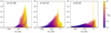 |
Fig. 1. Pixel distribution functions of all the simulations in the Loreli II database, illustrating the variety of possible shapes. The color of each individual curve depends on the fX value for the corresponding simulation. |
Another possibility is to use the statistical moments of the PDF computed from the cubes as:  , where Npix is the number of pixels and xi their positions. We note that these moments are centered because we subtracted the mean of the signal from the cubes. One possible difficulty with using these summary statistics is that, if we want five of them, from m2 to m6, we must raise the noised δTb value to powers up to 6, making our statistics sensitive to outliers. An alternative to the mk are the linear moments (Hosking 1990), defined as follows. Considering n independent samples from the distribution, we denote Xr : n the rth smallest value in the samples. Then the linear moment, lk, is defined as:
 (2)
(2)
We can check, for example, that l2 is proportional to the expectation of the largest minus expectation of the smallest in samples of two draws; thus, it is a measure of the width of the distribution. In the same manner, upper linear moments estimate properties of the distribution similar to those estimated by traditional statistical moments, but without resorting to raising the sample to powers larger than 1. They are thus expected to be less sensitive to outliers and to yield lower variance estimators. Generally speaking, when used as targets for the inference, lower variance statistics are expected to produce more constraining posteriors on the model parameters. As computing the lk is significantly more expensive than the mk, we used the Fortran routines provided by Hosking (1996), which we have found to be hundreds of times faster than the available Python version. We used moments l2 to l6, evaluating their performances for inference compared to moments m2 to m6, then compared and combined them with the power spectrum.
We note that the statistical moments and the power spectrum are not fully independent summary statistics: for example, m2 is the variance of the signal and thus very much correlated with the sum of the power spectrum. Indeed, our goal is not to maximise information with a minimal number of summary statistics, but to demonstrate the possibility to combine them with SBI and reach tighter constraints on the model parameters.
3. Simulation-based inference with neural density estimators
3.1. Principle
The principle of SBI is presented for example in Alsing et al. (2019). The fundamental idea is that a complete model, including stochastic processes such as cosmic variance or instrumental noise, is able to simulate some observed data d (a noised 21 cm cube in our case) from the set of parameters θ (those described in Section 2.2 in our case). Then, each pass forward of the model produces a pair (θ, d), which is a sampling of the underlying joint distribution of θ and d, or given θ, a sampling of the likelihood P(d|θ). In many cases, we did not have an analytic expression of the true likelihood, as we did, for example, for the PDF moments. However, given a large number of such samples, we can attempt to fit a parametric function to the true likelihood. As the parameters of the fitting function will depend (in the general case) on θ, the fitting procedure will require many samples for θ. Moreover, even a simple multivariate Gaussian parametric likelihood will involve (n + 2)(n + 1)/2 fitting parameters in the case of a vector of data with n components. In our case with vectors of 15 or 30 components, this means fitting 120 or 496 parameters. Consequently the task of finding the best fit is entrusted to a neural density estimator (NDE), which often takes the form of a simple multi-layer perceptron. It takes as input the (θ, d) pairs and produces the θ-dependent values of the parameters of the parameterised likelihood function. The information provided by d will only be used during training to converge to the correct fitting parameters values. We denote LTrue(d|θ) the true, unknown likelihood, while LNDE(d|θ, αi) is the parametric likelihood that can be estimated from the output of the NDE. The αi values are the outputs of the NDE and functions of θ and of the NDE weight. Thus, training the NDE means minimising the difference between LTrue and LNDE. This difference can be quantified with the Kullback–Liebler divergence:
 (3)
(3)
The evaluation of the integral can be replaced by a summation on the available samples: the probability that each sample was generated is accounted for by the LTrue(d|θ) factor before the logarithm in the integral. Since we are working to minimise the KL with respect to the αi, the numerator term in the logarithm that does not depend on the αi can be ignored. Then, our goal is to find:
 (4)
(4)
This quantity can be readily computed for a set of (θi, di) and used as a loss for the NDE, which will adjust its weights to produce the αi that minimise this loss.
3.2. Inference framework
3.2.1. General set-up
The first and possibly most important design element when building the NDE framework is the choice of the parametric form for the likelihood function. The most basic choice is a multivariate Gaussian. Indeed, our observables are summary statistics that are typically combinations of many physical quantities affected by stochastic processes. From the central limit theorem, we would generally expect them to exhibit near-Gaussian distributions. However, we are not necessarily able to compute analytically the parameters of these distributions (e.g. for the PDF moments) and even less so their full covariance matrix when the summary statistics are correlated. This is why SBI is meaningful even with a simple multivariate Gaussian parameterisation. However, to better account for departures from the Gaussian behaviour, we can use Gaussian mixture models (GMMs) or masked autoregressive flows (MAFs, Alsing et al. 2019; Prelogović & Mesinger 2023). However, Prelogović & Mesinger (2023) did not find a clear improvement from using MAFs to perform inference on the power spectrum. Moreover, Meriot et al. (2024) found that with the Loreli II database and thermal noise resulting from 100 hours of SKA observations, a simple multivariate Gaussian likelihood for the power spectrum performs best. In this work, we use the PDF, which is able to encode non-Gaussian behaviours, as a target for the inference, consequently the results presented here were all obtained with a two-component GMM. The observed lack of improvement beyond two components did not motivate us to explore MAFs.
We decided to carry out the inference process for the transformed parameters: log10(fx), log10(τ), rH/S, log10(Mmin), and fesc. This is consistent with a regular sampling in the Loreli II database. We report our findings in terms of these quantities normalised to the [0, 1] interval. The sampled 5D volume serves as our prior (see in Meriot et al. 2024 how it differs from a hypercube in the (τ, Mmin) plane). The prior is flat inside the sampled volume and zero outside. As is typical in the case of neural networks, we benefit a great deal from the normalisation of all the data, so we also need to normalise the observable quantities. For the (noised) power spectrum, we first applied the P(k, z)→log10(1 + P(k, z)) transformation, then, individually for each of the 15 different (ki, zj) pairs used for the inference, we normalise the data to the [0, 1] interval using the minimum and maximum values found across the whole range of noised signal in the database. We do the same for the lk moments of the PDF, without the log(1 + x) transformation. The same normalisation does not work for mk moments that are much more sensitive to outliers. In this case, we first need to compute the mean and variance of the distribution of mk across the database and proceed with a linear transformation to bring the values from the [μ − 2σ, μ + 2σ] interval to the [0, 1] interval.
3.2.2. Designing and training the NDE
With our choice for the form of the parametric likelihood, the NDE is trained to minimise the following loss:
![Mathematical equation: $$ \begin{aligned} \mathrm{Loss}=-\log \left[\sum _{k = 1}^{N_{\rm c}} {{ w}_k \over \sqrt{(2 \pi )^{N_{\rm obs}} \mathrm{det} (\Sigma })} e^{-{{1 \over 2}(\mathbf d -\boldsymbol{\mu })^T\Sigma ^{-1}(\mathbf d -\boldsymbol{\mu })}}\right] , \end{aligned} $$](/articles/aa/full_html/2025/06/aa53115-24/aa53115-24-eq9.gif) (5)
(5)
where Nc is the number of components in the mixture model, Nobs the dimension of the vector of summary statistics, wk the weights of the components as predicted by the NDE, μ the vector of the means of the summary statistics predicted by the NDE, and Σ the covariance matrix of the summary statistics. The NDE does not predict directly the covariance matrix, but the coefficients of the triangular matrix C, which is related to the inverse of the covariance matrix by the Cholesky decomposition: Σ−1 = CCT. Predicting C automatically ensures that Σ is definite-positive. In the general case, wk, μ, and Σ are functions of the input parameters.
The architecture of the NDE is described in Fig. 2 and implemented with the Keras-tensorflow framework. In our configuration, using a deeper network or increasing the number of neurons in the layers did not result in a decreased validation loss. The training sample is made of 90% of the simulations in Loreli II selected at random. For each simulation, 1000 different realisations of the instrumental noise were added to the 21 cm cubes and the summary statistics were computed from the noised cubes, resulting in ∼8 × 10⁶ samples. The remaining ten per cent of simulations were used for validation. The Nadam optimiser was used with an initial learning rate of 0.0002. A small batch size of 4 samples gives a lower loss, while further reducing the batch size is prohibitive in terms of efficiency. We first trained the networks by providing the ∼8 × 10⁶ samples once, then we decrease the learning rate by a factor of 10 and performed a retraining on half of the samples to improve convergence. The loss function did not decrease any more beyond that point.
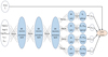 |
Fig. 2. Architecture of the neural network used for the NDEs. The inputs are the model parameters and the summary statistics of a corresponding noised signal and the outputs allow us to evaluate the parametric likelihood function of the summary statistics (see main text). For each layer (blue regions), we give the number of neurons and the activation function. Then, Nc is the number of components of the GMM describing the likelihood, Nobs is the length of the vector of summary statistics, and |
Using the final value of the validation loss is a usual measure of the quality of the training of the network, however, in our case, this must be handled with care. Indeed, given the form of our loss function, its value depends on the choice of normalisation of the summary statistics, which changes the covariance matrix, Σ. Changing the dimension of the summary statistics vector also changes the final loss value. Moreover we do not have a known lower bound of the loss as if, for example, we were using a mean-squared error loss. Thus, while in some cases we can tell that one network performs better than another, we cannot tell from the loss value how well it performs on an absolute scale. We have to turn to a much more costly evaluation of the performances: simulation-based calibration (SBC).
3.2.3. MCMC sampler
Once the NDEs are trained they can be used in a classical MCMC framework to compute the likelihood of the target signal at each step of the chain. Even if the cost of each likelihood computation is just a few milliseconds, computing 105 − 106 steps sequentially represents a non-negligible cost for a single inference. To speed up the process, we used the EMCEE sampler (Goodman & Weare 2010), which involves creating a team of 160 walkers that can be advanced simultaneously in the parameter space. Moreover, we used a custom implementation of EMCEE rather than a standard Python package. Indeed, when the likelihood function involves a forward pass in a neural network, it is important to use rather large batches of inputs for good compute performance. Passing a likelihood function that involves a neural network to the usual Python implementation of EMCEE results in batches of size 1 and can be up to 30 times slower than our custom implementation where the batch size is half the number of walkers.
3.3. Validating the framework with Simulation Based Calibration
The difficulty in using machine learning to perform Bayesian inference is to evaluate the validity of the resulting posteriors. The methods can be tested on toy models where the posterior is known analytically but there is no guarantee that satisfactory convergence will extend to cases where the model is more complex. SBC is a partial answer to the validation issue. It is presented in Talts et al. (2018) and applied to the 21-cm signal inference in Prelogović & Mesinger (2023) and Meriot et al. (2024): it validates the shapes of the marginalised 1D posteriors (noting, however, that two different posteriors in higher dimension can still produce identical 1D marginalisations).
The principle of SBC is to check a fundamental property of posterior distributions. A given observed signal, affected by a stochastic realisation of the noise, can be reproduced with different values of the model parameters. Some values are less likely than others as they require an extreme and unlikely realisation of the noise to match the observed signal, while others have a higher probability. In practice the true parameter value that produced the observed signal will fall outside the 1-sigma interval of the posterior in 32% of the cases, simply because the observed signal was affected by a rather unlikely noise realisation. More generally, the true parameters will fall with equal probability in each equal-sized quantile interval of the true posterior. SBC is aimed at testing this property for the posteriors obtained with SBI.
To perform this test, we could use many noised realisations of the signal arising from a single parameter value, compute the posterior for each of them, find the quantile interval of the posterior the true parameter values falls into, and compute a histogram of the quantile interval populations. A flat histogram means a successful test. This would however validate the inference framework at a single location in parameter space. Instead, we use noised signals produced with the different true parameter values in the Loreli II database: the resulting histogram should still be flat and the test probes the full volume of the explored parameter space.
As this test is statistical in nature, it requires a large number of inferences on different signals (summary statistics in our case). To find in which quantile interval of the corresponding 1D marginalised posterior each parameter θi falls, we examined the MCMC chain computed during the inference (after removing the burn-in phase). We computed the rank statistics of θi among all the values in the chain (the rank statistics simply count how many values in the chain are smaller than θi). It is then trivial to deduce the quantile interval from the rank statistics. Following this type of analysis for a large number of inferences, we have the capacity to build an histogram of the resulting population of the quantile intervals.
We estimated the validity of the inferences performed with four different NDEs that have been trained for inference, respectively, on the power spectrum, the mk PDF moments, the lk PDF moments, and the combination of power spectrum and lk moments. As learning near the sharp edges of Loreli II prior in parameter space is a more difficult task for the NDE, we selected 908 simulations not located near the boundary of the prior, performed the inference with all four NDEs, and computed the quantile intervals histograms. The results are presented in Fig. 3. The first obvious conclusion is that the inference on fesc is strongly under-confident: too many true fesc values fall near the median of the posterior (0.5 value of the x axis). This unsatisfactory result is understandable since only three different values of fesc are sampled in Loreli II. Since we excluded the boundary values, all the simulations used for the SBC have the same fesc. We are obviously in a regime where our sampling of the parameter space is not dense enough to run an SBC test comfortably. The second conclusion is that the NDE trained to infer on the mk moments does not perform as well as the others. In particular, the marginalised posteriors for log10(Fx) and log10(Mmin) are more biased. This is revealed by the tilted histograms: the true value of the parameter falls more often on one side of the median of the computed posterior. One possible explanation is that the higher sensitivity of the mk moments to outliers makes it more difficult for the NDE to learn the likelihood.
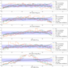 |
Fig. 3. Histograms over the 908 inferences describing where the true parameter values fall in the cumulative distribution function of the 1D marginalised posteriors. One histogram is plotted for each different NDE. If the posteriors match the true unknown posteriors the histogram should be flat. A toy model is plotted for comparison where the approximate posterior is a biased or under-confident normal distribution and the true posterior is the normal distribution. |
The other cases (power spectrum, lk moments, and combination of the two) show similar, rather satisfactory behaviours for parameters other than fesc. In comparison, the same diagnostic is computed in the cases where the estimated posterior is a Normal distribution with mean of 0 and standard deviation of 1 and the true posterior is either a Normal distribution with a mean of 0.2 and standard deviation of 1 (biased estimated posterior), or a Normal distribution with a mean of 0 and standard deviation of 0.85 (under-confident estimated posterior). We can see on the figure that a bias equal to ∼20% of the variance or a variance overestimated by ∼15% are reasonable estimations of the level of inaccuracy in the estimated marginalised posteriors. The higher dimensional data used by the NDE dealing with the combination of power spectrum and PDF moments do not seem to degrade the performance. Considering the uncertainties and approximations in the modelling of the 21-cm signal even with full radiative hydrodynamics simulations (see e.g. Semelin et al. 2023), along with the level of uncorrected systematics that currently plague the observations and that are not likely to completely disappear with the SKA, we consider the obtained level of accuracy satisfactory. Of course, if a thermal noise level consistent with 1000 hours of observation was used, the same inference framework may not yield sufficiently accurate posteriors.
4. Comparing and combining summary statistics
Since we found that the inference on fesc is not quite reliable, from now, we only report results on the other four parameters. We note that fesc is still varied in the MCMC chains. Also, since the NDE training with the mk moments performs the worst in terms of SBC, we mostly focus on the lk moments.
4.1. Individual posteriors
For the computation of the SBC diagnostics we performed 908 inferences on noised signals corresponding to different points in the parameter space. The resulting posteriors show a variety of behaviours and we cannot show them all here. However, before we present a statistical analysis of the results, we can see in Fig. 4 some examples of the result of the inference for four different signals.
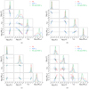 |
Fig. 4. Corner plot of the inferences done with the 3 NDEs on the different summary statistics for four different signals (one in each panel). The corresponding truth value of the parameters are indicated by the black dashed lines. Only the 1-sigma contours are plotted for clarity. |
Let us first insist on the fact that these inferences were performed on summary statistics affected by noise. Consequently, the true parameter values are not expected to match the maximum of the posteriors. Moreover, we also do not expect the true values to fall in the same quantile of the posteriors for all summary statistics, simply because these summary statistics are different and respond differently to a given noise realisation. We describe the four cases below.
Case (a) depicts a situation where inferring on the combination of power spectrum and PDF linear moments brings a significant tightening of the constraints on all parameters, compared to the inference on the power spectrum or the PDF linear moments separately. Case (b) is similar but with a less significant tightening of the constraints compared to the power spectrum. These behaviours are quite common in the 908 inferences as shown below in the statistical analysis. Case (c) shows an unusual case where constraints using the power spectrum alone are actually tighter than constraints, using the combination of power spectrum and PDF moments. This counter-intuitive situation could take place, for example, when adding the PDF moments shifts the median of the posterior towards a region of the parameter space where the signal intrinsically provides weaker constraints on the parameters. Alternatively, this may be a sign that the training of the NDEs are locally less accurate. Finally, case (d) shows a situation where the power spectrum posterior is bimodal and adding the information contained in the PDF moments lifts the ambiguity.
4.2. Statistical analysis
The question we want to answer relates to using the combination of power spectrum and linear moments of the PDF and whether this gives statistically tighter constraints on the parameters than using either of them alone. In the four-dimensional parameter space (excluding fesc from the analysis), the tightness of the constraints can be quantified by the square root of the so-called generalised variance:  , where Σ is the covariance matrix of the posterior that we can easily estimate from the MCMC chains. If the posterior is a multivariate Gaussian, V is proportional to the volume enclosed in the 1σ hyper-surface. In more general cases, it still characterises the volume encompassed by the posterior. The other obvious quantities that we can use are the standard deviations of the marginalised 1D posteriors. In Table 1, we report the median of all these quantities computed from the posteriors at the 908 different location in parameter space and using the different possible summary statistics as signals. The first and main conclusion is that in terms of the median values of the standard deviations, using the combination of the power spectrum and the linear moments of the PDF brings a tightening of constraints for all parameters of 20–30% and a factor more than 2.5 for the volume V of the 4D posterior. The second result is that the power spectrum produces tighter constraints than the PDF. Finally, the mk moments of the PDF perform slightly worse than the lk moments (noting, however, once again that the posteriors for the mk are also less reliable).
Posterior widths for different summary statistics.
We can see from Fig. 4 that in some cases, the inference on the power spectrum gives tighter constraints than on the combined statistics. To estimate if this is a common occurrence, Fig. 5 displays a scatter plot of  against
  for the 908 inferences. A dot below both the x = 1 and y = 1 lines indicates that the combined statistics outperforms both of the individual statistics. We can see that a small but non-negligible fraction (computed to be 8.5%) of the points in parameter space actually gives tighter constraints from an individual statistics (almost always the power spectrum). The figure also shows that the PDF alone does outperform the power spectrum alone (points above the y = x line) in 15% of the cases. Figure 6 shows the same plots but for the standard deviation of the 1D marginalised posteriors for each of the parameters. The fractions of cases were a single statistics outperform the combination is 19%, 25%, 33% and 21% for log10(fx), log10(τ), rH/S, and log10(Mmin) respectively. While these numbers are higher than for V (accounting for cases where only one or two parameters out of four are better constrained by the power spectrum or PDF alone), the overall result demonstrates that combining summary statistics produces a significant improvement on the constraints on the parameters by exploiting more information. This result can only be achieved with SBI.
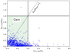 |
Fig. 5. Scatter plot of the ratios of the characteristic volume occupied by the 4D posteriors (see main text for definition). Each blue cross is an inference on a different noised signal. In the green region the combined statistics give a smaller volume than either of the individual statistics. |
 |
Fig. 6. Same as Fig. 5 but for the ratios of the volumes (i.e. standard deviation here) occupied by the 1D marginalised posteriors. |
5. Conclusion
SBI is a new development in Bayesian inference in general and it is a novel approach for the 21-cm signal in particular. As long as the inference is performed on data that actually obey a Gaussian likelihood, with known mean and variance (in response to stochastic processes such as instrumental noise), SBI will (in the best case, i.e. perfect neural network training) reproduce the result of traditional inference techniques such as MCMC. However, even for the 21-cm power spectrum, Prelogović & Mesinger (2023) showed that using the unknown full covariance matrix (discovered with an SBI approach) instead of only the known diagonal terms changes the results of the inference. Still, this does not have a major impact on the result as soon as a non-negligible level of thermal noise is included, thereby boosting the diagonal terms. However, since the signal is non-Gaussian, the power spectrum does not contain all the information. Unfortunately, we do not know the analytical form of the likelihood for other summary statistics, such as the PDF or scattering transform, and have no reason to assume that a Gaussian approximation would be satisfactory. If this additional information is to be used in an inference framework, it can be done only with SBI. This is also the case for combining correlated summary statistics, where the form of the correlations are not known analytically. This work and Prelogović & Mesinger (2024) show that such combinations tighten the constraints on astrophysical parameters. Finally, the training of the SBI inference networks requires about two orders of magnitude fewer simulation signals than traditional MCMC approaches. This allows us to preform the inference with complex and costly models, such as the one used to build the Loreli II database, where an MCMC approach would face a prohibitive cost.
In this work, we have used the Loreli II database of radiative hydrodynamics simulations of the 21 cm signal to perform simulation-based inference using Neural Density Estimators to model the likelihood with a two-component GMM. We considered the following summary statistics as targets: the power spectrum, the statistical moments of the PDF, linear moments of the PDF, and the combination of power spectrum and linear moments of the PDF. Using simulation-based calibration, we showed that in most cases the 1D marginalised posteriors are biased by no more than 20% of the variance and under-confident by no more than 15%. However, the marginalised posteriors on fesc were markedly under-confident because of the inadequate sampling of this parameter in Loreli II. In addition, posteriors using the statistical moments of the PDF were less accurate than the others. Then, we were able to show that combining summary statistics by performing a simultaneous inference on the power spectrum and linear moments of the PDF brings a tightening of the 1σ volume of the 4D posterior in 90% of the cases. For 1D marginalised posteriors, this tightening occurs in 70–80% of the cases and has a median amplitude of 20 to 30%.
The limitations of Loreli II for use in SBI are discussed in Meriot et al. (2024). Learning from Loreli I, the sampling steps were designed to match, on average, the standard deviation of the posteriors for 100 hours of SKA observation. A lower level of thermal noise may require a denser sampling and the more peaked likelihood function may not be as well fitted with a simple GMM, requiring the use of more expressive neural network architectures such as MAFs. Another limitation worth mentioning is that only the cosmic variance and the instrumental thermal noise were considered to be sources of stochasticity. A more realistic model would also include stochasticity in the source formation process at scales that have not been resolved in the simulations, originating in the chaotic nature of the dynamics of galaxy formation and evolution on long timescales. These limitations come down to a simple fact that we must always keep in mind: the result of an inference may be valid given the underlying model, but its usefulness is still limited by the validity of the model itself.
Acknowledgments
The Loreli II database used in this work was build using computer and storage resources provided by GENCI at TGCC thanks to the grants 2022-A0130413759 and 2023-A0150413759 on the supercomputer Joliot Curie’s ROME partition.
References
- Abdurashidova, Z., Aguirre, J. E., Alexander, P., et al. 2022, ApJ, 924, 51 [NASA ADS] [CrossRef] [Google Scholar]
- Acharya, A., Mertens, F., Ciardi, B., et al. 2024, MNRAS, 534, L30 [Google Scholar]
- Alsing, J., & Wandelt, B. 2018, MNRAS, 476, L60 [NASA ADS] [CrossRef] [Google Scholar]
- Alsing, J., Charnock, T., Feeney, S., & Wandelt, B. 2019, MNRAS, 488, 4440 [Google Scholar]
- Baek, S., Di Matteo, P., Semelin, B., Combes, F., & Revaz, Y. 2009, A&A, 495, 389 [NASA ADS] [CrossRef] [EDP Sciences] [Google Scholar]
- Baek, S., Semelin, B., Di Matteo, P., Revaz, Y., & Combes, F. 2010, A&A, 523, A4 [NASA ADS] [CrossRef] [EDP Sciences] [Google Scholar]
- Barnes, J., & Hut, P. 1986, Nature, 324 [Google Scholar]
- Bowman, J. D., Rogers, A. E. E., Monsalve, R. A., Mozdzen, T. J., & Mahesh, N. 2018, Nature, 555, 67 [Google Scholar]
- Charnock, T., Lavaux, G., & Wandelt, B. D. 2018, Phys. Rev. D, 97, 083004 [NASA ADS] [CrossRef] [Google Scholar]
- Chuzhoy, L., & Zheng, Z. 2007, ApJ, 670, 912 [NASA ADS] [CrossRef] [Google Scholar]
- Ciardi, B., Ferrara, A., & White, S. D. M. 2003, MNRAS, 344, 7 [Google Scholar]
- Goodman, J., & Weare, J. 2010, Commun. Appl. Math. Comput. Sci., 5, 65 [Google Scholar]
- Gorce, A., & Pritchard, J. R. 2019, MNRAS, 489, 1321 [NASA ADS] [CrossRef] [Google Scholar]
- Greig, B., & Mesinger, A. 2015, MNRAS, 449, 4246 [NASA ADS] [CrossRef] [Google Scholar]
- Greig, B., Ting, Y.-S., & Kaurov, A. A. 2022, MNRAS, 513, 1719 [NASA ADS] [CrossRef] [Google Scholar]
- Harker, G., Zaroubi, S., Bernardi, G., et al. 2009, MNRAS, 397, 1138 [NASA ADS] [CrossRef] [Google Scholar]
- Hosking, J. R. M. 1996, RC20525, B, 52, 105 [Google Scholar]
- Hosking, J. R. M. 1990, J. Royal Statist. Soc., B52, 105 [Google Scholar]
- Hothi, I., Allys, E., Semelin, B., & Boulanger, F. 2024, A&A, 686, A212 [NASA ADS] [CrossRef] [EDP Sciences] [Google Scholar]
- Hutter, A., Watkinson, C. A., Seiler, J., et al. 2020, MNRAS, 492, 653 [CrossRef] [Google Scholar]
- Ichikawa, K., Barkana, R., Iliev, I. T., Mellema, G., & Shapiro, P. R. 2010, MNRAS, 406, 2521 [NASA ADS] [CrossRef] [Google Scholar]
- Lacey, C., & Cole, S. 1993, MNRAS, 262, 627 [NASA ADS] [CrossRef] [Google Scholar]
- Majumdar, S., Pritchard, J. R., Mondal, R., et al. 2018, MNRAS, 476, 4007 [NASA ADS] [CrossRef] [Google Scholar]
- McQuinn, M., Zahn, O., Zaldarriaga, M., Hernquist, L., & Furlanetto, S. R. 2006, ApJ, 653, 815 [NASA ADS] [CrossRef] [Google Scholar]
- Mellema, G., Iliev, I. T., Alvarez, M., & Shapiro, P. R. 2006, New Astron., 11, 374 [NASA ADS] [CrossRef] [Google Scholar]
- Meriot, R., & Semelin, B. 2024, A&A, 683, A24 [NASA ADS] [CrossRef] [EDP Sciences] [Google Scholar]
- Meriot, R., Semelin, B., & Cornu, D. 2024, A&A, in press, https://doi.org/10.1051/0004-6361/202452901 [Google Scholar]
- Mertens, F. G., Bobin, J., & Carucci, I. P. 2024, MNRAS, 527, 3517 [Google Scholar]
- Mittal, S., Kulkarni, G., & Garel, T. 2024, MNRAS, 535, 1979 [Google Scholar]
- Monaghan, J. J. 1992, ARA&A, 30, 543 [NASA ADS] [CrossRef] [Google Scholar]
- Munshi, S., Mertens, F. G., Koopmans, L. V. E., et al. 2024, A&A, 681, A62 [NASA ADS] [CrossRef] [EDP Sciences] [Google Scholar]
- Papamakarios, G., & Murray, I. 2016, ArXiv e-prints [arXiv:1605.06376] [Google Scholar]
- Prelogović, D., & Mesinger, A. 2023, MNRAS, 524, 4239 [CrossRef] [Google Scholar]
- Prelogović, D., & Mesinger, A. 2024, A&A, 688, A199 [NASA ADS] [CrossRef] [EDP Sciences] [Google Scholar]
- Reis, I., Fialkov, A., & Barkana, R. 2021, MNRAS, 506, 5479 [NASA ADS] [CrossRef] [Google Scholar]
- Rubiño-Martín, J. A., Betancort-Rijo, J., & Patiri, S. G. 2008, MNRAS, 386, 2181 [CrossRef] [Google Scholar]
- Saxena, A., Meerburg, P. D., Weniger, C., Acedo, E. D. L., & Handley, W. 2024, RAS Tech. Instrum., 3, 724 [Google Scholar]
- Semelin, B. 2016, MNRAS, 455, 962 [NASA ADS] [CrossRef] [Google Scholar]
- Semelin, B., & Combes, F. 2002, A&A, 495, 389 [Google Scholar]
- Semelin, B., Combes, F., & Baek, S. 2007, A&A, 495, 389 [NASA ADS] [Google Scholar]
- Semelin, B., Eames, E., Bolgar, F., & Caillat, M. 2017, MNRAS, 472, 4508 [NASA ADS] [CrossRef] [Google Scholar]
- Semelin, B., Mériot, R., Mertens, F., et al. 2023, A&A, 672, A162 [NASA ADS] [CrossRef] [EDP Sciences] [Google Scholar]
- Shimabukuro, H., Yoshiura, S., Takahashi, K., Yokoyama, S., & Ichiki, K. 2016, MNRAS, 458, 3003 [NASA ADS] [CrossRef] [Google Scholar]
- Singh, S., Jishnu, N. T., Subrahmanyan, R., et al. 2022, Nat. Astron., 6, 607 [NASA ADS] [CrossRef] [Google Scholar]
- Talts, S., Betancourt, M., Simpson, D., Vehtari, A., & Gelman, A. 2018, ArXiv e-prints [arXiv:1804.06788] [Google Scholar]
- Watkinson, C. A., Majumdar, S., Pritchard, J. R., & Mondal, R. 2017, MNRAS, 472, 2436 [NASA ADS] [CrossRef] [Google Scholar]
- Yoshiura, S., Pindor, B., Line, J. L. B., et al. 2021, MNRAS, 505, 4775 [CrossRef] [Google Scholar]
- Zhao, X., Mao, Y., Cheng, C., & Wandelt, B. D. 2022, ApJ, 926, 151 [NASA ADS] [CrossRef] [Google Scholar]
- Zhao, X., Mao, Y., Zuo, S., & Wandelt, B. D. 2024, ApJ, 973, 41 [Google Scholar]
All Tables
All Figures
|
Fig. 1. Pixel distribution functions of all the simulations in the Loreli II database, illustrating the variety of possible shapes. The color of each individual curve depends on the fX value for the corresponding simulation. |
| In the text | |
|
Fig. 2. Architecture of the neural network used for the NDEs. The inputs are the model parameters and the summary statistics of a corresponding noised signal and the outputs allow us to evaluate the parametric likelihood function of the summary statistics (see main text). For each layer (blue regions), we give the number of neurons and the activation function. Then, Nc is the number of components of the GMM describing the likelihood, Nobs is the length of the vector of summary statistics, and |
| In the text | |
|
Fig. 3. Histograms over the 908 inferences describing where the true parameter values fall in the cumulative distribution function of the 1D marginalised posteriors. One histogram is plotted for each different NDE. If the posteriors match the true unknown posteriors the histogram should be flat. A toy model is plotted for comparison where the approximate posterior is a biased or under-confident normal distribution and the true posterior is the normal distribution. |
| In the text | |
|
Fig. 4. Corner plot of the inferences done with the 3 NDEs on the different summary statistics for four different signals (one in each panel). The corresponding truth value of the parameters are indicated by the black dashed lines. Only the 1-sigma contours are plotted for clarity. |
| In the text | |
|
Fig. 5. Scatter plot of the ratios of the characteristic volume occupied by the 4D posteriors (see main text for definition). Each blue cross is an inference on a different noised signal. In the green region the combined statistics give a smaller volume than either of the individual statistics. |
| In the text | |
|
Fig. 6. Same as Fig. 5 but for the ratios of the volumes (i.e. standard deviation here) occupied by the 1D marginalised posteriors. |
| In the text | |
Current usage metrics show cumulative count of Article Views (full-text article views including HTML views, PDF and ePub downloads, according to the available data) and Abstracts Views on Vision4Press platform.
Data correspond to usage on the plateform after 2015. The current usage metrics is available 48-96 hours after online publication and is updated daily on week days.
Initial download of the metrics may take a while.