| Issue |
A&A
Volume 686, June 2024
|
|
|---|---|---|
| Article Number | A133 | |
| Number of page(s) | 13 | |
| Section | Numerical methods and codes | |
| DOI | https://doi.org/10.1051/0004-6361/202449214 | |
| Published online | 06 June 2024 | |
Simulation-based inference with neural posterior estimation applied to X-ray spectral fitting
Demonstration of working principles down to the Poisson regime
Institut de Recherche en Astrophysique et Planétologie,
9 avenue du Colonel Roche,
Toulouse
31028, France
e-mail: This email address is being protected from spambots. You need JavaScript enabled to view it.
Received:
11
January
2023
Accepted:
19
February
2024
Abstract
Context. Neural networks are being extensively used for modeling data, especially in the case where no likelihood can be formulated.
Aims. Although in the case of X-ray spectral fitting the likelihood is known, we aim to investigate the ability of neural networks to recover the model parameters and their associated uncertainties and to compare their performances with standard X-ray spectral fitting, whether following a frequentist or Bayesian approach.
Methods. We applied a simulation-based inference with neural posterior estimation (SBI-NPE) to X-ray spectra. We trained a network with simulated spectra generated from a multiparameter source emission model folded through an instrument response, so that it learns the mapping between the simulated spectra and their parameters and returns the posterior distribution. The model parameters are sampled from a predefined prior distribution. To maximize the efficiency of the training of the neural network, while limiting the size of the training sample to speed up the inference, we introduce a way to reduce the range of the priors, either through a classifier or a coarse and quick inference of one or multiple observations. For the sake of demonstrating working principles, we applied the technique to data generated from and recorded by the NICER X-ray instrument, which is a medium-resolution X-ray spectrometer covering the 0.2–12 keV band. We consider here simple X-ray emission models with up to five parameters.
Results. SBI-NPE is demonstrated to work equally well as standard X-ray spectral fitting, both in the Gaussian and Poisson regimes, on simulated and real data, yielding fully consistent results in terms of best-fit parameters and posterior distributions. The inference time is comparable to or smaller than the one needed for Bayesian inference when involving the computation of large Markov chain Monte Carlo chains to derive the posterior distributions. On the other hand, once properly trained, an amortized SBI-NPE network generates the posterior distributions in no time (less than 1 second per spectrum on a 6-core laptop). We show that SBI-NPE is less sensitive to local minima trapping than standard fit statistic minimization techniques. With a simple model, we find that the neural network can be trained equally well on dimension-reduced spectra via a principal component decomposition, leading to a faster inference time with no significant degradation of the posteriors.
Conclusions. We show that simulation-based inference with neural posterior estimation is a complementary tool for X-ray spectral analysis. The technique is robust and produces well-calibrated posterior distributions. It holds great potential for its integration in pipelines developed for processing large data sets. The code developed to demonstrate the first working principles of the technique introduced here is released through a Python package called SIXSA (Simulation-based Inference for X-ray Spectral Analysis), which is available from GitHub.
Key words: methods: data analysis / methods: numerical / methods: statistical / techniques: spectroscopic
© The Authors 2024
 Open Access article, published by EDP Sciences, under the terms of the Creative Commons Attribution License (https://creativecommons.org/licenses/by/4.0), which permits unrestricted use, distribution, and reproduction in any medium, provided the original work is properly cited.
This article is published in open access under the Subscribe to Open model. This email address is being protected from spambots. You need JavaScript enabled to view it. to support open access publication.
1 Introduction
X-ray spectral fitting generally relies on frequentist and Bayesian approaches (see Buchner & Boorman 2024 for a recent and comprehensive review on the statistical aspects of X-ray spectral analysis). Fitting X-ray spectra with neural networks was introduced by Ichinohe et al. (2018) for the analysis of high spectral resolution galaxy cluster spectra, and recently by Parker et al. (2022) for the analysis of lower resolution Athena Wide Field Imager spectra of active galactic nuclei. Parker et al. (2022) showed that neural networks delivered comparable accuracy to spectral fitting while limiting the risk of outliers caused by the fit becoming stuck in a local false minimum (which anyone involved in X-ray spectral fitting dreads); yet, they offer an improvement of around three orders of magnitude in speed, once the network is properly trained. On the other hand, no error estimates on the spectral parameter were provided in the methods explored by Parker et al. (2022).
In a Bayesian framework, accessing the posterior distribution is possible through the simulation-based inference with neural posterior estimation methodology (hereafter SBI-NPE; Papamakarios & Murray 2016; Lueckmann et al. 2017; Greenberg et al. 2019; Deistler et al. 2022a; see also Cranmer et al. 2020 for a review of simulation-based inference). In this approach, we sample parameters from a prior distribution and generate synthetic spectra from these parameters. Those spectra are then fed to a neural network that learns the association between simulated spectra and the model parameters. The trained network is then applied to data, to derive the parameter space consistent with the data and the prior, being the posterior distribution. In contrast to conventional Bayesian inference, SBI is also applicable when one can run model simulations, but no formula or algorithm exists for evaluating the likelihood of data given the parameters.
Simulation based inference with neural posterior estimation has demonstrated its power across many fields, including astrophysics, in reconstructing galaxy spectra and inferring their physical parameters (Khullar et al. 2022), in inferring variability parameters from dead-time-affected light curves (Huppenkothen & Bachetti 2022), in exoplanet atmospheric retrieval (Vasist et al. 2023), in deciphering the ring down phase signal of the black hole merger GW150914 (Crisostomi et al. 2023), and, very recently, in isolated pulsar population synthesis (Graber et al. 2023).
In this paper, we demonstrate the power of SBI-NPE for X-ray spectral fitting for the first time, showing that it delivers performances fully consistent with the XSPEC (Arnaud 1996) and the Bayesian X-ray Analysis (BXA) spectral fitting packages (Buchner et al. 2014), which are two of the most commonly used tools for X-ray fitting. The paper is organized as follows. In Sect. 2, we give some more insights into the SBI-NPE method. In Sect. 3, we present the methodology to produce the simulated data, introducing a method to reduce the prior range. In Sect. 4, we show examples of single-round inference in the Gaussian and Poisson regimes for simulated mock data. In Sect. 5, we present a case based on multiple-round inference. In Sect. 6, we demonstrate the robustness of the technique against local minima trapping. In Sect. 7, using a simple model, we apply the principal component analysis to reduce the data fed to the network. In Sect. 8, we show the performance of SBI-NPE on real data, as recorded by the NICER X-ray instrument (Gendreau et al. 2012). In Sect. 9, we discuss the main results of the paper, listing some avenues for further investigations. This precedes a short conclusion.
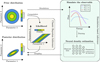 |
Fig. 1 Simulation-based inference approach emulates traditional Bayesian inference approach. When assessing the parameters of a model, one first defines prior distributions and then defines the likelihood of a given observation, often using a forward-modeling approach. This likelihood is further sampled to obtain the posterior distribution of the parameters. The simulation-based approach does not require explicit computation of the likelihood, and instead it will learn an approximation of the desired distribution (i.e., the likelihood or directly the posterior distribution) by training a neural network with a sample of simulated observations. |
2 SBI with amortized neural posteriors
2.1 Formalism
The SBI approach, illustrated in Fig. 1, is aimed at computing the probability distribution of interest, in this case the posterior distribution p(θ|x), by learning an approximation of the probability density function from a joint sample of parameters {θi} and the associated simulated observable {xi}, using neural density estimators such as normalizing flow. A normalizing flow T is a diffeomorphism between two random variables, say X and U, which links their following density functions as follows:
 (1)
(1)
where JT is the Jacobian matrix of the normalizing flow. The main idea when using normalizing flows is to define a transformation between a simple distribution (i.e., normal distribution) and the probability distribution that should be modeled, which eases the manipulation of such functions. To achieve this, an option is to compose several transformations Ti to form the overall normalizing flow T, each parameterized using masked auto-encoders for density estimation (MADE; Germain et al. 2015), which are based on deep neural networks. MADEs satisfy the auto-regressive properties necessary to define a normalizing flow and can be trained to adjust to the desired probability density. Stacking several MADEs will form what is defined as a masked auto-regressive flow (MAF; Papamakarios et al. 2017). We refer interested readers to the following reviews by Papamakarios et al. (2021) and Kobyzev et al. (2021). Greenberg et al. (2019) developed a methodology that enabled the use of MAFs to directly learn the posterior distribution of a Bayesian inference problem, using a finite set of parameters and associated observable {θi, xi}. Using this approach, one can compute an approximation for the posterior distribution q(θ, x) ≃ p(θ|x), which can be used to obtain samples of spectral model parameters from the posterior distribution conditioned on an observed X-ray spectrum.
The python scripts from which the results presented here use the sbi1 package (Tejero-Cantero et al. 2020). sbi is a Py Torch-based package that implements SBI algorithms based on neural networks. It eases inference on black-box simulators by providing a unified interface to state-of-the-art algorithms together with very detailed documentation and tutorials. It is straightforward to use, involving the use of just a few Python functions.
Amortized inference enables the evaluation of the posterior for different observations without having to re-run inference. On the other hand, multiple-round inference focuses on a particular observation. At each round, samples from the obtained posterior distribution computed at the observation are used to generate a new training set for the network, yielding in a better approximation of the true posterior at the observation. Although fewer simulations are needed, the major drawback is that the inference is no longer amortized, it being specific to an observation. We discuss both approaches in the sections below.
2.2 Bench-marking against the known likelihood
Simulation based inference implements machine learning techniques in situations where the likelihood is undefined, hampering the use of conventional statistical approaches. In our case, the likelihood is known. Here, we recall the basic equations. Taking the notation of XSPEC (Arnaud 1996), the likelihood of Poisson data (assuming no background) is known as
 (2)
(2)
where Si are the observed counts in the bin i as recorded by the instrument, t is the exposure time over which the data were accumulated, and mi are the predicted count rates based on the current model and the response of the instrument folding in, its instrument efficiency, its spectral resolution, its spectral coverage, and so on (see Buchner & Boorman 2024 for details on the folding process). The associated negative log-likelihood, given in Cash (1979) and often referred to as the Cash-statistic, is
 (3)
(3)
The final term that depends exclusively on the data (and hence does not influence the best-fit parameters) is replaced by Stirling’s approximation to give
 (4)
(4)
This is what is used for the statistic C-STAT option in XSPEC. The best-fit model is the one that leads to the lowest C-STAT2. The default XSPEC minimization method uses the modified Levenberg-Marquardt algorithm based on the CURFIT routine from Bevington & Robinson (2003). In the following sections, we use XSPEC with and without Bayesian inference and compute Markov chain Monte Carlo (MCMC) chains to obtain the parameter probability distribution and compute errors on the best-fit parameters to enable a direct comparison with the posterior distributions derived from SBI-NPE. By default, we use the Goodman-Weare algorithm (Goodman & Weare 2010) with eight walkers, a burn-in phase of 5000, and a length of 50 000. The analysis was performed with the pyxspec wrapper of XSPEC v.12.13.1 (Arnaud 1996).
In addition to XSPEC, we used the Bayesian X-ray analysis (BXA) software package (Buchner et al. 2014) to validate our results. Among many useful features, BXA connects XSPEC to the nested sampling algorithm as implemented in UltraNest (Buchner 2021) for Bayesian Parameter Estimation. BXA finds the best fit and computes the associated error bars and marginal probability distributions (see Buchner & Boorman 2024 for a comprehensive tutorial on BXA). We run the BXA solver with default parameters; however, we note that there are different options to speed up BXA, including the possibility to parallelize BXA over multiple cores, as discussed in Buchner & Boorman (2024).
We now introduce a method to restrict the prior range, with the objective of providing the network a training sample that is not too far from the targeted observation(s). This derives in part from the challenge, that for this work the generation of spectra, the inference, the generation of the posteriors should be performed on a MacBook Pro 2.9 GHz 6-Core Intel Core i9, within a reasonable amount of time.
3 Generating an efficient training sample
The density of the training sample depends on the range of the priors and the number of simulations. As the training time increases with the size of the training sample, ideally one would train the network with a limited number of simulated spectra that are not too far from the targeted observation(s), yet fully cover the observation(s). Here, we consider two methods to restrict the priors: one in which we train a network to retain the “good” samples of θi matching a certain criterion (Sect. 3.2), and one in which we perform a coarse inference of the targeted observation(s) (Sect. 3.3).
3.1 Simulation set-up
We first describe our simulation set-up. We assume a simple emission model consisting of an absorbed power law with three parameters: the column density (NH), the photon index (gamma, Γ), and the normalization of the power law at 1 keV (NormPL). We used the tbabs model to take into account interstellar absorption, including the photoelectric cross-sections and the element abundances to the values provided by Verner et al. (1996) and Wilms et al. (2000), respectively. In XSPEC terminology, the model is tbabs*Powerlaw. For the simulations, we used NICER response files (the observation identified in the NICER HEASARC archive as OBSID1050300108 is referenced later in the paper). The simulated spectra are grouped in five consecutive channels so that each spectrum has ~200 bins covering the 0.3 and 10 keV range. The initial range of priors is given in Table 1 for the model 1 set-up. We assume uniform priors in linear coordinates for NH and for Γ and in logarithmic coordinates for the power-law normalization. The generation of synthetic spectra is done within jaxspec3, which offers paral-lelization of a fakeit-like command in XSPEC (Dupourqué et al., in prep.). The generation of 10 000 simulations takes about ten seconds (including a few seconds of just-in-time compilation). In this first work, we did not consider instrumental background. However, we note that if a proper analytical model exists for the background, the network could be trained to learn about the source and the background spectra simultaneously (with more free model parameters than in the source-alone case). This would come at the expense of increasing the size of the training sample, hence inference time. The background spectrum could also be incorporated simply as a nuisance parameter, by adding to each bin of each simulated spectrum a number of counts with an empirical distribution estimated from the background spectrum. This would increase the dispersion in the spectrum, which would translate into an additional source of variance on the constraints of the model parameters. More details on this approach will be provided in a forthcoming paper by Dupourqué et al. (in prep.).
Prior assumption for emission models considered.
3.2 A restricted prior
For the first method, we train a ResNet classifier (He et al. 2015) to restrict the prior distributions (Lueckmann et al. 2017; Deistler et al. 2022b). sbi can be used to learn regions of the parameter space producing valid simulations and to distinguish them from regions that lead to invalid simulations. The process can be iterative; we expect that, as more simulations are fed to the classifier, the rejection rate will increase and the restricted prior will shrink. It can be stopped when the fraction of valid simulations exceeds a given threshold, depending on the criterion. In all cases, we recommend performing sanity checks of the coverage of the restricted prior for the observation(s) to fit. The user has to define a decision criterion for the classifier. To demonstrate the working principle of SBI-NPE under various statistical regimes (total number of counts in the X-ray spectra; see below), the first criterion we chose is to restrict the total number of counts in the spectra within a given range. Secondly, we also considered a criterion such that the valid simulations are the ones providing the lowest C-STAT computed from the observation to fit (Cash 1979). Once the simulations are produced, the classifier is also very fast (minute timescales), depending on the condition to match and the number of model parameters and size of the training sample (as an indication, for the three parameter model considered below, a few thousands simulations are required). We note that such a classifier is straightforward to implement and could be coupled with classical X-ray spectral fitting, to initialize the fit closer to the best-fit solution, and thus reduce the likelihood of becoming stuck in a local false minimum.
The first statistical regime to be probed is the so-called high-count Gaussian regime. We define the integration time of the simulated spectra that is identical to all spectra and defined such that a reference model (NH = 0.2 × 1022 cm−2, Gamma = 1.7, and NormPL =1) corresponds to a spectrum with about 20 000 counts (over 200 bins). This provides the reference spectrum (referred to as Spectrum20000counts). We define the criterion for the restrictor, such that the valid simulations are the ones which have between 10 000 and 100 000 counts, ensuring that the reference spectrum (Spectrum20000counts) is well covered. In Fig. 2, we show the initial and final round of the restricted prior, derived with the above criterion. Given the integration time for the spectra, only a restricted set of model parameters (mostly the normalization of the power-law component) can deliver the right number of counts per spectrum.
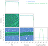 |
Fig. 2 Initial and restricted priors tuned to produce spectra that have between 10 000 and 100 000 counts for a tbabs*powerlaw model (at its tenth iteration). As expected, only a restricted range of the power-law normalization can deliver the right number of counts. |
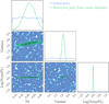 |
Fig. 3 Initial and restricted priors computed from a coarse and quick inference of a reference spectrum of 20 000 counts. Such a coarse inference can be seen as the first step of a multiple-round inference. |
3.3 Coarse inference
The second method uses a coarse inference and can be considered as the first step in a multiple-round inference. A coarse inference is when the network is trained with a limited number of samples (see Sect. 4.1 for the parameters used to run the inference). The posterior conditioned at the reference observation is then used as the restricted prior. In Fig. 3, we present the result of a coarse inference of the above reference spectrum (Spectrum20000counts). Five thousand spectra are generated from the initial prior as defined in Table 1 for the above model, fed to the neural network, and the posterior distributions are computed at the reference spectrum. The training for such a limited sample of simulations, for three parameters, takes about one minute. As can be seen, the prior range is further constrained to narrower intervals. Generating a sample of 10 000 spectra with parameters from this restricted prior shows that the reference spectrum is actually close to the median of the sample of the simulated spectra (see Fig. 4). The robustness of SBI-NPE against local false minima trapping (see Sect. 6) guarantees good coverage of the observation from the restricted prior.
4 Single-round inference
Starting from the restricted prior, one can then draw samples of θi and generate spectra applying the Poisson count statistics in each spectral bin. The spectra are then binned the same way as the reference observation (grouped by 5 adjacent channels between 0.3 and 10 keV), and injected as such in the network (no zero mean scaling, no component reduction applied; see, however, Sect. 7). For each run, we generate both a training and an independent test sample.
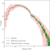 |
Fig. 4 Prior predictive check showing that coarse inference provides good coverage of reference spectrum (Spectrum20000counts). The coverage of the restricted prior is indicated in red. The median of the spectra sampled from the restrictor (blue line) is to be compared with the reference spectrum (green line). |
4.1 In the Gaussian regime
In the first case, we run the classifier with the criterion that each of the simulated spectra assuming an absorbed power-law model having from 10 000–100 000 counts, spread over ~200 bins, are valid simulations. This covers the Gaussian regime. For three parameters, we generate a set of 10000 spectra. The network is trained in ~3 min. The inference is performed with the default parameters of SNPE_C as implemented in sbi, which uses five consecutive MADEs with 50 hidden states each for the density estimation. It then takes about the same time to draw 20 000 posterior samples for 500 test spectra, i.e. to fit 500 different spectra with the same network. The inferred model parameters versus the input parameters are shown in Fig. 5. As can be seen, there is an excellent match between the input and output parameters: the linear regression coefficient is very close to one. For NH, a minimal bias is observed toward the edge of the sampled parameter space.
We generate the posterior distributions for the reference absorbed power-law spectrum and compare it with the posterior distribution obtained from XSPEC by switching Bayesian inference4. The comparison is shown in Fig. 6. There is an excellent match between the best-fit parameters, but also the posterior distribution, including their spread. In both cases, the C-STAT of the best fit is within 1σ of the expected C-STAT following Kaastra (2017). We note that running XSPEC to derive the posterior distribution takes about the same time as training the network.
In the above case, we computed the goodness of the fit by comparing the measured fit statistic with its expected value following Kaastra (2017). XSPEC offers the possibility to perform a Monte Carlo calculation of the goodness of fit (goodness command), applicable in the case when the only source of variance in the data is counting statistics. This command simulates a number of spectra based on the model and returns the percentage of these simulations with the test statistic less than that for the data. If the observed spectrum is produced by the model then this number should be around 50%. XSPEC can generate simulated spectra either from the best-fit parameters or from a Gaussian distribution centered on the best fit, with sigma computed from the diagonal elements of the covariance matrix. XSPEC can either fit each simulated spectrum or return the fit statistic calculated immediately after creating the simulated spectrum. Fitting the data is the option by default, but at the expense of increasing the run time. Such a feature would be straightforward to implement with SBI-NPE and amortized inference. The set of parameters of the simulated spectra can be drawn from the posterior distribution conditioned at the observation, and the posterior distributions for each simulated spectrum can be computed from the already trained amortized network (the fit statistic associated with each simulated spectrum is as usual derived from the median of the so-computed posterior distributions). With the simulation set-up considered here, generating the simulated spectra and the posterior distributions is very fast (a few minutes for 1000 spectra).
We now show the count spectrum corresponding to the reference spectrum of this run, together with the folded model and the associated residuals (Fig. 7, for both SBI-NPE and XSPEC). As expected from Fig. 6, there is an excellent agreement between the fits with the two methods.
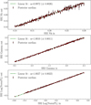 |
Fig. 5 Inferred model parameters versus input model parameters for the case in which spectra have between 10 000–100 000 counts, spread over 200 bins. A single round inference is performed on an initial sample of 10 000 simulated spectra. The median of the posterior distributions is computed from 20 000 samples and the error on the median is computed from the 68% quantile of the distribution. The linear regression coefficient is computed for each parameter over the 500 test samples. |
4.2 In the Poisson regime
The above results can be considered as encouraging, but to test the robustness of the technique, we must probe the low count Poisson regime. We repeat the run above, but this time generating spectra from a restricted prior generating 200 bin spectra with a number of counts ranging from 1000 to 10 000 for the absorbed power-law model. The integration time of the spectra is scaled down from the Gaussian case, so that the reference model (NH = 0.2 × 1022 cm−2, Gamma = 1.7 and NormPL = 1) now corresponds to a spectrum of ~2000 counts (referred as Spectrum2000counts). To account for the lower statistics, we train the network with a sample of 20 000 spectra, instead of 10 000 as in the case above. The training time is still about three minutes. We generate the posterior for a test set of 500 spectra, and this again takes about three minutes. Similar to Fig. 5, we show the input and inferred model parameters for the test sample in Fig. 8. As in the previous case, although with larger error bars, accounting for the lower statistics of the spectra, there is an excellent match between the two quantities, the linear regression coefficient remains close to 1, with some evidence of the small bias on NH at both ends of the parameter range being increased.
We generate the Posterior distribution for the reference spectrum (Spectrum2000counts), which we also fit with BXA (assuming the same priors as listed in Table 1 for the model 1 setup). The posterior distributions are compared in Fig. 9, showing again an excellent agreement. Not only are the best-fit parameters consistent with one another, but the widths of the posterior distribution are also comparable, which is equally important. This demonstrates that SBI-NPE generates healthy posteriors. We note that the time to run BXA (with the default solver parameters and without parallelization) on such a spectrum is comparable with the training time of the network.
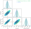 |
Fig. 6 Posterior distribution estimated for reference absorbed power-law spectrum (Spectrum20000counts) as inferred from a single-round inference with a network trained on 10 000 samples (green). The posterior distribution inferred from a Bayesian fit with XSPEC is also shown in blue. |
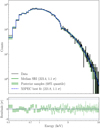 |
Fig. 7 Illustration of single-round inference for X-ray spectral fitting. Top: Count spectrum corresponding to reference absorbed power-law spectrum (Spectrum20000counts), together with the folded best-fit model from both SBI-NPE (green solid line) and XSPEC (blue dashed line). Bottom: Residuals of the best fit from SBI-NPE. |
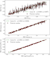 |
Fig. 8 Inferred model parameters versus input model parameters for case in which spectra have from 1000–10 000 counts spread over 200 bins. The neural network is trained with 20 000 simulations and the posteriors for 500 test spectra are then computed. The medians of the posteriors are computed from 20 000 samples, and the error on the median is computed from the 68% quantile of the distribution. The linear regression coefficient is computed for each parameter over the 500 test samples. |
5 Multiple-round inference
In the previous cases, the posterior is inferred using single-round inference. We are now considering multiple-round inference, tuned for a specific observation; the reference spectrum of 2000 counts, spread over 200 bins (Spectrum2000counts). For the first iteration, from the restricted prior, we generate 1000 simulations and train the network to estimate the posterior distribution. In each new round of inference, samples from the obtained posterior distribution conditioned at the observation (instead of from the prior) are used to simulate a new training set used for training the network again. This process can be repeated an arbitrary number of times. Here, we stop after three iterations. The whole procedure takes about 1.5 min. In Fig. 10, we show that multiple-round inference returns best fit parameters and posterior distributions consistent with single-round inference (from a larger training sample) and XSPEC. We thus confirm that multiple-round inference can be more efficient than single-round inference in the number of simulations and is faster in terms of inference time. Its drawback is, however, that the inference is no longer amortized (i.e., it will only apply for a specific observation).
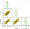 |
Fig. 9 Posterior distributions for reference spectrum of 2000 counts as derived from SBI-NPE with a single-round inference of a network trained with 20 000 samples (green) and by BXA in orange. |
6 Sensitivity to local minima
Fit statistic minimization algorithms may become stuck in local false minima. There are different workarounds, such as computing the errors on the model parameters to explore a wider parameter space, shaking the fits with different sets of initial parameters, using Bayesian inference, all at the expense of increasing the processing times. This is probably the reason why fit statistic minimization remains widely used, despite its known limitations. This makes worth the comparison of the sensitivity to local minima of SBI-NPE with XSPEC. For this purpose, we now consider a five-parameter model combining two overlapping components: a power law and a black body. In the XSPEC terminology, the model would be tbabs*(powerlaw+blackbody) (see Table 1 for the model 2 simulation set-up for the priors). We build a restricted prior so that such a model produces at least 10 000 counts per spectrum, as decent statistics is required to constrain a five-model parameter. We train a network with 100 000 simulated spectra. We then generate the posterior of 500 spectra that we fit with XSPEC with three sets of initial parameters: the model parameters, a set of model parameters generated from the restricted prior, and a set of model parameters from the initial prior (that do not meet necessarily our requirement on counts). We switch off Bayesian inference in the XSPEC fits, and we return the best-fit C-STER statistics for each of the fits. In Fig. 11, we compare the C-STAR of SBI-NPE as derived from a single-round inference with the XSPEC fitting. This figure shows that SBI-NPE does not produce outliers, while the minimization does, at the level of a few percent. The latter is a known fact. The use of a restricted prior helps in reducing the trapping in local false minima (compared to considering the wider original prior) because the XSPEC fits start closer to the best-fit parameters. The most favorable, yet unrealistic, situation for XSPEC is when the fit starts from the model parameters. In some cases, SBI-NPE produces minimum C-STATs that are slightly larger than those derived from XSPEC, indicating that the best-fit solution was not reached. This may simply call for enlarging the training sample of the network for such a five-parameter model, or considering multiple-round inference.
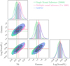 |
Fig. 10 Posterior distributions for reference spectrum of 2000 counts as derived from SBI-NPE with a single-round inference of a network trained with 20 000 samples (green); a multiple-round inference with three iterations in which the network is trained with a sample of 1000 simulations (pink); and by XSPEC (blue). |
7 Dimension reduction with the principal component analysis
Parker et al. (2022) introduced the use of principal component analysis (PCA) to reduce the dimension of the data to feed the neural network and showed that it increased the accuracy of the parameter estimation without any penalty on computational time; yet it enabled simpler network architecture to be used. The PCA performs a linear dimension reduction using singular value decomposition of the data to project it to a lower dimensional space. Unlike Parker et al. (2022), we have access to the posteriors, and it is worth investigating whether such a PCA decomposition affects the uncertainty on the parameter estimates. Considering the run presented in Sect. 4 for the case of single-round inference in the Poisson regime, we decompose the 20 000 spectra with the PCA, so as to keep 90% of their variance (before that, we scale the spectra to have a mean of 0 and standard deviation of 1). This allows us to reduce the dimension of the data from 20 000 × 200 to 20 000 × 60, i.e., a factor of three reduction, leading to a gain in inference time by a factor of two. In Fig. 12, we show the input and output parameters from a single-round inference trained on dimension-reduced data. As can be seen, there is still an excellent agreement between the two, with the linear regression coefficient close to one, although the bias on NH at the edge of the prior interval seems to be more pronounced (the slopes for all parameters are less than 1, indicating that a small bias may have been introduced through the PCA decomposition). We show the posteriors of the fit of the reference spectrum of 2000 counts in comparison with XSPEC in Fig. 13; this demonstrates that the posteriors are not broadened by the dimension reduction.
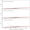 |
Fig. 11 Comparison between XSPEC spectral fitting (fit statistic minimization) and SBI-NPE. The initial parameters of the XSPEC fits are the input model parameter (top panel), a set of parameters generated from the restricted prior (middle panel), and a set of parameters generated from the initial prior (bottom panel). The y-scale is the same for the three panels. Outliers away from the red line are due to XSPEC becoming trapped in a local false minimum. |
8 Application to real data
Having shown the power of the technique on mock simulated data, it now remains to demonstrate its applicability to real data, recorded by an instrument observing a celestial source of X-rays (and not data generated by the same simulator used to train the network). This is a crucial step in machine learning applications.
We considered NICER response files for the above simulations because we are now going to apply the technique to real NICER data recorded from 4U 1820-303 (Gendreau et al. 2012; Keek et al. 2018). For the scope of the paper, we considered two cases: a spectrum for the persistent X-ray emission (number of counts ~200 000) and spectra recorded over a type I X-ray burst, when the X-ray emission shows extreme time and spectral variability.
8.1 NICER data analysis
We retrieved the archival data of 4U 1820-303 from HEASARC for the observation identifier (1050300108) and processed them with standard filtering criteria with the ni cer12 script provided as part of the HEAS0FTV6.31.1 software suite, as recommended from the NICER data analysis web page (NICER software version : NICER_2022-12-16_V010a). Similarly, the latest calibration files of the instrument are used throughout this paper (reference from the CALDB database is xti20221001). A light curve was produced between the 0.3 and 7 keV bands, with a time resolution of 120 ms, so the type I X-ray burst could be located precisely.
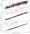 |
Fig. 12 Inferred model parameters versus input model parameters for case in which spectra have from 1000–10 000 counts spread over 200 bins. The best-fit parameters are derived from a single-round inference of a network trained by 20 000 samples, reduced by the PCA, so that only 90% of the variance in the samples is kept. |
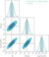 |
Fig. 13 Posterior distributions for reference spectrum of 2000 counts as derived from SBI-NPE with a single-round inference of a network trained with 20 000 samples (green) decomposed by the PCA (green: dimension reduced by a factor of 3) and XSPEC (blue). |
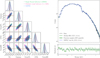 |
Fig. 14 A comparison of the best-fit results derived from single-round, multiple-round inference and XSPEC. Left: posterior distribution comparison between XSPEC spectral fitting and SBI-NPE, as applied to the persistent emission spectrum of 4U1820-303 (pre-burst). The spectrum is modeled as tbabs*(blackbody+powerlaw). There is a perfect match between the three methods, not only on the best fit parameters, but also on the width of the posterior distributions. Right: count spectrum of the persistent emission, together with the folded model derived from both SBI-NPE and XSPEC. The C-STAR of the best fit is indicated together with its deviation against the expected value. |
8.2 Spectrum of the persistent emission
Once the burst time was located, we first extracted a spectrum of the persistent emission for 200 s, ending ten seconds before the burst. The spectrum is then modeled by a five-component model, as the sum of an absorbed black-body plus power law. In XSPEC terminology, the model is tbabs*(blackbody+powerlaw). The initial range of prior is given in Table 1 for the model 2 setup. For both SBI-NPE and XSPEC spectral fitting, conversely, we consider uniform priors in linear coordinates for all the parameters. Similarly, for this observation, we build a restricted prior with the criterion that the classifier keeps 25% of the model parameters associated with the lowest C-STAR (considering a set of 5000 simulations for 5 parameters). From this restricted prior, we generate a rather conservative set of 100 000 spectra for a single-round inference and a set of 5000 spectra for a multiple-round inference considering only three iterations. It takes about 40 minutes to train the network with 100 000 spectra with five parameters, and 12 min for the three-iteration multiple-round inference. The posterior distribution from single and multiple-round inference and the XSPEC fitting are shown in Fig. 14, together with the folded spectrum and best fit residuals. As can be seen, there is a perfect match between XSPEC and SBI-NPE, demonstrating that the method is also applicable to real data. We verified that changing the assumptions for the priors (e.g., uniform in logarithmic scale for the normalizations of both the black body and the power law) yielded fully consistent results in terms of best-fit parameters, C-STAR, and posterior distributions.
The same applies when using BXA instead of XSPEC. This is the first demonstration to date that SBI-NPE performs equally well as state-of-the-art X-ray fitting techniques on real data.
8.3 The burst emission
The first burst observed with NICER was reported by Keek et al. (2018), Strohmayer et al. (2019), and Wenhui et al. (2024). The burst emission is fit with a black-body model and a component accounting for some underlying emission, which in our case is assumed to be a simple power law. The black-body temperature and its normalization vary strongly along the burst itself, in particular in this burst, which showed the so-called photospheric expansion, meaning that the temperature of the black body drops while its normalization increases, to raise again toward the end of the burst. To follow spectral evolution along the burst, we extract fixed-duration spectra (0.25 s), still grouped in five adjacent channels, so that all the spectra have the same number of bins (200). The number of counts per spectrum ranges from 400 to 5000, hence offering the capability of exploring the technique with real data in the Poisson regime. In this range of statistics, we do not attempt to constrain a five-parameter model. Hence, we fix the column density and the power-law index to NH = 0.2 × 1022 cm−2 and Γ = 1.7, respectively. The initial range of prior is given in Table 1 for the model 3 set-up.
As we want to use the power of amortized inference, we use two methods to define our training sample. First, we apply the classifier with the condition of keeping the model parameters associated with spectra with a number of counts ranging from 100–10 000 and hence fully covering the range of counts of the observed spectra (400–5000). From the restricted prior, we arbitrarily consider 5000 simulated spectra per observed spectrum so that the network is trained with 23 × 5000 = 115 000 samples. Second, we perform a coarse inference over the full prior range, and, for each of the 23 spectra, we set the restricted prior as the posterior conditioned at the corresponding spectrum. The training sample is limited to 10 000 spectra for the quick and coarse inference of the 23 spectra. For each of the 23 restricted prior, we then generate 2500 simulated spectra so that as a whole they can be used tso train the network (i.e., with 23 × 2500 = 57 500 samples). The predictive check of this prior is shown in Fig. 15, which indicates that such a build-up prior covers all the observed spectra. The training then takes ~15 min. The generation of the posterior samples takes ~20 s. We then fit the data with Bayesian inference with XSPEC. Next, we derive the errors on the fit parameters using a MCMC method. As can be seen from Fig. 15, SBI-NPE with amortized inference for the two different restricted priors can follow the spectral evolution along the burst, with a level of accuracy comparable to XSPEC, even when the number of counts in the spectra goes down to a few hundred, deep into the Poisson regime. The results of our fits are fully consistent with those reported by Keek et al. (2018), Strohmayer et al. (2019) and Wenhui et al. (2024). This further demonstrates that SBI-NPE is applicable to real data and that the power of amortization can still be used for multiple spectra showing wide variability.
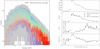 |
Fig. 15 Application of SBI-NPE to real NICER data. Left: 23 burst spectra covered by the restricted prior, indicated by the region in gray. Right: recovered spectral parameters with SBI-NPE and XSPEC. The agreement between the different methods is remarkable. The figure shows the number of counts per spectrum (top), the normalization of the power law, the temperature of the back body in keV, and at the bottom the black-body normalization translated to a radius (in km) assuming a distance to the source of 8 kpc. Single-round inference is performed with a training sample of 23 × 5000 spectra, derived from a restrictor, constraining the number of counts in the spectra to be between 100 and 10 000 counts (red filled circles). Single-round inference is also performed with a training sample of 23 × 2500 spectra, generated from a restrictor build from a quick inference (green filled circles). XSPEC best-fit results are shown with blue filled circles. |
9 Discussion
We demonstrated the first working principles of SBI-NPE for X-ray spectral fitting for both simulated and real data. We showed that it can not only recover the same best-fit parameters as traditional X-ray fitting techniques, but also delivers healthy posteriors comparable to those derived from Bayesian inference with XSPEC and BXA. The method works equally well in the Gaussian and Poisson regimes, with uncertainties reflecting the statistical quality of the data. The existence of a known likelihood helps to demonstrate that the method is well calibrated. We still performed recommended checks such as simulation-based calibrations (SBCs; Talts et al. 2018), which is a procedure for validating inferences from Bayesian algorithms capable of generating posterior samples. SBC provides a (qualitative) view and a quantitative measure to check whether the uncertainties of the posterior are well-balanced (i.e., neither over-confident nor under-confident). SBI-NPE as implemented here passed the SBC checks, as expected from the comparison of the posterior distributions with XSPEC and BXA.
We showed SBI-NPE to be less sensitive to local false minima than classical minimization techniques as implemented in XSPEC, consistently with the findings of Parker et al. (2022). We showed that, although raw spectra can train the network, SBI-NPE can be coupled with principal component analysis to reduce the dimensions of the data to train the network, offering potential speed improvements for the inference (Parker et al. 2022). For the simple models considered here, no broadening of the posterior distribution is observed. This kind of approach can be extended to various dimension reduction methods since SBI-NPE is not bound to any likelihood computation. The latter also means that SBI-NPE could apply when formulating a likelihood is not optimal, e.g. in the case of the analysis of multidimensional Poisson data of extended X-ray sources (Peterson et al. 2004).
Multiple-round inference combined with a restricted prior is perfectly suited when dealing with just a few observations. The power of amortization can also be used, even when the observations show large spectral variability, as demonstrated above. The consideration of a restricted prior, either on the interval of counts covered by the observation data sets or from a coarse fitting of the ensemble of observations with a neural network trained on a small sample of spectra used upfront, makes it possible to define an efficient training sample, to cover the targeted observations. We note, however, that the use of a restricted prior can always be compensated by a larger sample size on an extended prior, with the penalty being on the training time. The use of a classifier to restrict the range of priors, which is easy to implement and fast running, can be coupled with standard X-ray fitting tools to increase their speed and decrease the risk of being trapped in local false minima.
Within the demonstration of the working principles of the technique, we found that the training time of the neural network is shorter and/or comparable to state-of-the-art fitting tools. Speeding up the training may be possible using more powerful computers, e.g. moving from a laptop to a cluster. On the other hand, once the network has been trained, generating the posterior distribution is instantaneous, and orders of magnitude faster than traditional fitting. This means that SBI-NPE holds great potential for integration in pipelines of data processing for massive data sets. The range of applications of the method has yet to be explored, but the ability to process a large sample of observations with the same network offers the opportunity to use it to track instrument dis-functioning, calibration errors, and so on. This will be investigated for the X-IFU instrument on Athena (Barret et al. 2023).
We are aware that we demonstrated the working principles of SBI-NPE (considering simple models) spectra with a relatively small number of bins. The applicability of the technique to more sophistical models and higher resolution spectra (such as those that will be provided by X-IFU) will have to be demonstrated, although the alternative tools, such as XSPEC and BXA, may have issues of their own in terms of processing time. Through this demonstration, we have already identified some aspects of the technique to keep investigating. For instance, an amortized network is applicable to an ensemble of spectra that must have the same grouping, the same exposure time, and so on. The latter could be relaxed if one is not interested in the normalization of the model components (flux), but just the variations of the other parameters (e.g., the index of a power law). Alternatively, the posterior distributions of the normalizations of each of the additive components of the models could be scaled afterwards to account for the different integration times, with respect to the integration time of the simulated spectra used for the training. On the other hand, there is no easy way to work around the case of spectra with different numbers of bins. This will require some further investigation. Obviously, there are many cases where meaningful information can still be derived considering similar grouping and integration time for the spectra, as we show above in the case of a type I X-ray burst. Once the network has been trained, the generation of posteriors being instantaneous, SBI-NPE makes it possible to track model parameter variations on timescales much shorter than those possible today with existing tools.
The quality of the training depends on the size of the training sample. Caution is therefore recommended when lowering the sample size to increase the inference speed. It should be stated again that when using amortized inference, the time to train the network will always be compensated afterwards by the order-of-magnitude-faster generation of the posteriors for a large number of spectra. There is no rule to define the minimum sample size yet. Similarly, for multiple-round inference, the number of iterations is a free parameter, which may need some fine-tuning to ensure that convergence to the best-fit solution has been reached. The existence of alternative robust tools such as XSPEC and BXA will help to define guidelines. For complex multi-component spectra, the size of the training sample will have to be increased. The use of a restricted prior will always help; however, considering dimension reduction (e.g. decomposition in principal components) or the use of an embedding network to extract the relevant summary features of the data may become mandatory. Any loss of information will have an impact on the inference itself. Another limitation may come from the time to generate the simulations to train the network. In our work, we used simple models and a fully parallel version of the XSPEC fakeit developed within jaxspec (Dupourqué et al., in prep.). This was not a limiting factor for this work, as generating thousands of simulations takes only a few seconds.
The python scripts from which the results were derived are based on the sbi package (Tejero-Cantero et al. 2020). With this paper, we release the simulation-based inference for X-ray spectral analysis (SIXSA)5 python package, from which the working principles of single and multiple-round inference with neural posterior estimation have been demonstrated. The python scripts that come with reference spectra are straightforward to use and can be customized for different applications. We also release a first version of jaxspec to further support the development and use of SBI-NPE for X-ray spectral fitting. We note that jaxspec is currently limited in the number of models available (only basic analytical models, as the ones used here, are available). It obviously remains possible to generate and use simulated spectra produced with software packages such as XSPEC. This is encouraged, in particular for testing SBI-NPE with a large number of model parameters.
10 Conclusions and future advances
We demonstrated the working principles of fitting X-ray spectra with simulation-based inference with neural posterior estimation, down to the Poisson regime, for the first time. We applied the technique to real data and demonstrated that SBI-NPE converges to the same best-fit parameters and provides fitting errors comparable to Bayesian inference. We may therefore be at the eve of a new era for X-ray spectral fitting, but more work is needed to demonstrate the wider applicability of the technique to more sophisticated models and higher resolution spectra, and in particular to those provided by the new generation of instruments, such as the X-IFU spectrometer to fly on-board Athena. Yet, along this work, we do not identify any difficulties for this not to be achievable. Certainly, the pace at which machine learning applications develop across so many fields will also help in solving any issues that we may have to face, further strengthening the case for developing the potential of simulation-based inference with neural posterior estimation for X-ray spectral fitting. The release of the SIXSA python package should help the community to contribute to this exciting prospect.
Acknowledgements
D.B. would like to thank all the colleagues who shared their unfortunate experience of getting stuck, without knowing, into local false minima, when doing X-ray spectral fitting. The fear of ignoring that the true global minimum is just nearby is what motivated this work in the first place with the hope of preventing sleepless nights in the future. D.B. is also grateful to all his X-IFU colleagues, in particular from CNES, for developing such a beautiful instrument that will require new tools, such as the one introduced here, for analyzing the high quality data that it will generate. D.B./S.D. thank Alexei Molin and Erwan Quintin for their support and encouragements along this work. The authors are grateful to Fabio Acero, Maggie Lieu, the anonymous referee and the editor for useful comments on the paper. Finally D.B. thanks Michael Deistler for support in using and optimizing the restricted prior. In addition to the sbi package (Tejero-Cantero et al. 2020), this work made use of many awesome Python packages: ChainConsumer (Hinton 2016), matplotlib (Hunter 2007), numpy (Harris et al. 2020), pandas (McKinney 2010), pytorch (Paszke et al. 2017), scikit-learn (Pedregosa et al. 2011), scypi (Virtanen et al. 2020), tensorflow (Abadi et al. 2016). Link to the software The simulation-based inference for X-ray spectral analysis (SIXSA) python package is available at: https://github.com/dbxifu/SIXSA.
References
- Abadi, M., Agarwal, A., Barham, P., et al. 2016, arXiv e-prints [arXiv:1603.04467] [Google Scholar]
- Arnaud, K. A. 1996, ASP Conf. Ser., 101, 17 [Google Scholar]
- Barret, D., Albouys, V., Herder, J.-W. D., et al. 2023, Exp. Astron., 55, 373 [NASA ADS] [CrossRef] [Google Scholar]
- Bevington, P., & Robinson, D. 2003, Data Reduction and Error Analysis for the Physical Sciences (New York: McGraw-Hill Education) [Google Scholar]
- Bradbury, J., Frostig, R., Hawkins, P., et al. 2018, http://github.com/google/jax [Google Scholar]
- Buchner, J. 2021, J. Open Source Softw., 6, 3001 [CrossRef] [Google Scholar]
- Buchner, J., & Boorman, P. 2024, Statistical Aspects of X-ray Spectral Analysis, eds. C. Bambi, & A. Santangelo (Singapore: Springer Nature Singapore), 5403 [Google Scholar]
- Buchner, J., Georgakakis, A., Nandra, K., et al. 2014, A&A, 564, A125 [NASA ADS] [CrossRef] [EDP Sciences] [Google Scholar]
- Cash, W. 1979, ApJ, 228, 939 [Google Scholar]
- Cranmer, K., Brehmer, J., & Louppe, G. 2020, Proc. Natl. Acad. Sci., 117, 30055 [Google Scholar]
- Crisostomi, M., Dey, K., Barausse, E., & Trotta, R. 2023, Phys. Rev. D, 108, 044029 [CrossRef] [Google Scholar]
- Deistler, M., Goncalves, P. J., & Macke, J. H. 2022a, arXiv e-prints [arXiv:2210.04815] [Google Scholar]
- Deistler, M., Macke, J. H., & Gonçalves, P. J. 2022b, Proc. Natl. Acad. Sci., 119, e2207632119 [NASA ADS] [CrossRef] [Google Scholar]
- Gendreau, K. C., Arzoumanian, Z., & Okajima, T. 2012, SPIE Conf. Ser., 8443, 844313 [Google Scholar]
- Germain, M., Gregor, K., Murray, I., & Larochelle, H. 2015, Proc. Int. Conf. Mach. Learn., 881, 1938 [Google Scholar]
- Goodman, J., & Weare, J. 2010, Commun. Appl. Math. Comput. Sci., 5, 65 [Google Scholar]
- Graber, V., Ronchi, M., Pardo-Araujo, C., & Rea, N. 2023, ApJ, submitted [arXiv:2312.14848] [Google Scholar]
- Greenberg, D. S., Nonnenmacher, M., & Macke, J. H. 2019, arXiv e-prints [arXiv:1905.07488] [Google Scholar]
- Harris, C. R., Millman, K. J., van der Walt, S. J., et al. 2020, Nature, 585, 357 [NASA ADS] [CrossRef] [Google Scholar]
- He, K., Zhang, X., Ren, S., & Sun, J. 2015, arXiv e-prints [arXiv:1512.03385] [Google Scholar]
- Hinton, S. R. 2016, J. Open Source Softw., 1, 00045 [NASA ADS] [CrossRef] [Google Scholar]
- Hoffman, M. D., & Gelman, A. 2014, J. Mach. Learn. Res., 15, 1593 [Google Scholar]
- Hunter, J. D. 2007, Comput. Sci. Eng., 9, 90 [NASA ADS] [CrossRef] [Google Scholar]
- Huppenkothen, D., & Bachetti, M. 2022, MNRAS, 511, 5689 [NASA ADS] [CrossRef] [Google Scholar]
- Ichinohe, Y., Yamada, S., Miyazaki, N., & Saito, S. 2018, MNRAS, 475, 4739 [NASA ADS] [CrossRef] [Google Scholar]
- Kaastra, J. S. 2017, A&A, 605, A51 [NASA ADS] [CrossRef] [EDP Sciences] [Google Scholar]
- Keek, L., Arzoumanian, Z., Chakrabarty, D., et al. 2018, ApJ, 856, L37 [NASA ADS] [CrossRef] [Google Scholar]
- Khullar, G., Nord, B., Ćiprijanović, A., Poh, J., & Xu, F. 2022, Mach. Learn. Sci. Technol., 3, 04LT04 [CrossRef] [Google Scholar]
- Kobyzev, I., Prince, S. J. D., & Brubaker, M. A. 2021, IEEE Trans. Pattern Anal. Mach. Intell., 43, 3964 [NASA ADS] [CrossRef] [Google Scholar]
- Lueckmann, J.-M., Goncalves, P. J., Bassetto, G., et al. 2017, arXiv e-prints [arXiv:1711.01861] [Google Scholar]
- McKinney, W. 2010, in Proceedings of the 9th Python in Science Conference, eds. S. van der Walt, & J. Millman, 51 [Google Scholar]
- Papamakarios, G., & Murray, I. 2016, arXiv e-prints [arXiv:1605.06376] [Google Scholar]
- Papamakarios, G., Pavlakou, T., & Murray, I. 2017, in Advances in Neural Information Processing Systems (New York: Curran Associates, Inc.), 30 [Google Scholar]
- Papamakarios, G., Nalisnick, E., Rezende, D. J., Mohamed, S., & Lakshminarayanan, B. 2021, J. Mach. Learn. Res., 22, 1 [Google Scholar]
- Parker, M. L., Lieu, M., & Matzeu, G. A. 2022, MNRAS, 514, 4061 [NASA ADS] [CrossRef] [Google Scholar]
- Paszke, A., Gross, S., Chintala, S., et al. 2017, in 31st Conference on Neural Information Processing Systems (NIPS 2017), Long Beach, CA, USA [Google Scholar]
- Pedregosa, F., Varoquaux, G., Gramfort, A., et al. 2011, J. Mach. Learn. Res., 12, 2825 [Google Scholar]
- Peterson, J. R., Jernigan, J. G., & Kahn, S. M. 2004, ApJ, 615, 545 [NASA ADS] [CrossRef] [Google Scholar]
- Strohmayer, T. E., Altamirano, D., Arzoumanian, Z., et al. 2019, ApJ, 878, L27 [NASA ADS] [CrossRef] [Google Scholar]
- Talts, S., Betancourt, M., Simpson, D., Vehtari, A., & Gelman, A. 2018, arXiv e-prints [arXiv:1804.06788] [Google Scholar]
- Tejero-Cantero, A., Boelts, J., Deistler, M., et al. 2020, J. Open Source Softw., 5, 2505 [NASA ADS] [CrossRef] [Google Scholar]
- Vasist, M., Rozet, F., Absil, O., et al. 2023, A&A, 672, A147 [NASA ADS] [CrossRef] [EDP Sciences] [Google Scholar]
- Verner, D. A., Ferland, G. J., Korista, K. T., & Yakovlev, D. G. 1996, ApJ, 465, 487 [Google Scholar]
- Virtanen, P., Gommers, R., Oliphant, T. E., et al. 2020, Nat. Meth., 17, 261 [Google Scholar]
- Wenhui, Y., Zhaosheng, L., Yongqi, L., et al. 2024, A&A, 683, A93 [NASA ADS] [CrossRef] [EDP Sciences] [Google Scholar]
- Wilms, J., Allen, A., & McCray, R. 2000, ApJ, 542, 914 [Google Scholar]
In the Gaussian high-count regime, the χ2 statistic is often used in the fitting, but here we used C-STAT as it applies in both the Gaussian and Poisson regimes without any bias at low counts (e.g., Buchner & Boorman 2024).
jaxspec is a pure Python library for statistical inference on X-ray spectra. It allows us to easily build spectral models by combining components and fit it to one or multiple observed spectra. It builds on JAX (Bradbury et al. 2018) to enable computation on the GPU and just-intime compilation. The differentiable framework enables advanced sampling algorithms such as NUTS (Hoffman & Gelman 2014). The v0.0.2 of jaxspec, which was used in this work, is available at https://github.com/renecotyfanboy/jaxspec, along with the SIXSA package at https://github.com/dbxifu/SIXSA. More details will be available in Dupourqué et al. (in prep.).
XSPEC by default uses uniform priors for all parameters. For this run, we considered Jeffrey’s prior for the normalization of the power law instead of a log uniform distribution. XSPEC adds a contribution from the prior as –2 In Pprior to the fit statistic (Arnaud 1996, which in our case is a positive contribution equal to the 2 ln(NormPL)). Such a contribution is removed when comparing the results of XSPEC run with Bayesian inference, with the results of SBI-NPE. We note that in BXA, Jeffrey’s priors have been deprecated for log uniform priors.
All Tables
All Figures
|
Fig. 1 Simulation-based inference approach emulates traditional Bayesian inference approach. When assessing the parameters of a model, one first defines prior distributions and then defines the likelihood of a given observation, often using a forward-modeling approach. This likelihood is further sampled to obtain the posterior distribution of the parameters. The simulation-based approach does not require explicit computation of the likelihood, and instead it will learn an approximation of the desired distribution (i.e., the likelihood or directly the posterior distribution) by training a neural network with a sample of simulated observations. |
| In the text | |
|
Fig. 2 Initial and restricted priors tuned to produce spectra that have between 10 000 and 100 000 counts for a tbabs*powerlaw model (at its tenth iteration). As expected, only a restricted range of the power-law normalization can deliver the right number of counts. |
| In the text | |
|
Fig. 3 Initial and restricted priors computed from a coarse and quick inference of a reference spectrum of 20 000 counts. Such a coarse inference can be seen as the first step of a multiple-round inference. |
| In the text | |
|
Fig. 4 Prior predictive check showing that coarse inference provides good coverage of reference spectrum (Spectrum20000counts). The coverage of the restricted prior is indicated in red. The median of the spectra sampled from the restrictor (blue line) is to be compared with the reference spectrum (green line). |
| In the text | |
|
Fig. 5 Inferred model parameters versus input model parameters for the case in which spectra have between 10 000–100 000 counts, spread over 200 bins. A single round inference is performed on an initial sample of 10 000 simulated spectra. The median of the posterior distributions is computed from 20 000 samples and the error on the median is computed from the 68% quantile of the distribution. The linear regression coefficient is computed for each parameter over the 500 test samples. |
| In the text | |
|
Fig. 6 Posterior distribution estimated for reference absorbed power-law spectrum (Spectrum20000counts) as inferred from a single-round inference with a network trained on 10 000 samples (green). The posterior distribution inferred from a Bayesian fit with XSPEC is also shown in blue. |
| In the text | |
|
Fig. 7 Illustration of single-round inference for X-ray spectral fitting. Top: Count spectrum corresponding to reference absorbed power-law spectrum (Spectrum20000counts), together with the folded best-fit model from both SBI-NPE (green solid line) and XSPEC (blue dashed line). Bottom: Residuals of the best fit from SBI-NPE. |
| In the text | |
|
Fig. 8 Inferred model parameters versus input model parameters for case in which spectra have from 1000–10 000 counts spread over 200 bins. The neural network is trained with 20 000 simulations and the posteriors for 500 test spectra are then computed. The medians of the posteriors are computed from 20 000 samples, and the error on the median is computed from the 68% quantile of the distribution. The linear regression coefficient is computed for each parameter over the 500 test samples. |
| In the text | |
|
Fig. 9 Posterior distributions for reference spectrum of 2000 counts as derived from SBI-NPE with a single-round inference of a network trained with 20 000 samples (green) and by BXA in orange. |
| In the text | |
|
Fig. 10 Posterior distributions for reference spectrum of 2000 counts as derived from SBI-NPE with a single-round inference of a network trained with 20 000 samples (green); a multiple-round inference with three iterations in which the network is trained with a sample of 1000 simulations (pink); and by XSPEC (blue). |
| In the text | |
|
Fig. 11 Comparison between XSPEC spectral fitting (fit statistic minimization) and SBI-NPE. The initial parameters of the XSPEC fits are the input model parameter (top panel), a set of parameters generated from the restricted prior (middle panel), and a set of parameters generated from the initial prior (bottom panel). The y-scale is the same for the three panels. Outliers away from the red line are due to XSPEC becoming trapped in a local false minimum. |
| In the text | |
|
Fig. 12 Inferred model parameters versus input model parameters for case in which spectra have from 1000–10 000 counts spread over 200 bins. The best-fit parameters are derived from a single-round inference of a network trained by 20 000 samples, reduced by the PCA, so that only 90% of the variance in the samples is kept. |
| In the text | |
|
Fig. 13 Posterior distributions for reference spectrum of 2000 counts as derived from SBI-NPE with a single-round inference of a network trained with 20 000 samples (green) decomposed by the PCA (green: dimension reduced by a factor of 3) and XSPEC (blue). |
| In the text | |
|
Fig. 14 A comparison of the best-fit results derived from single-round, multiple-round inference and XSPEC. Left: posterior distribution comparison between XSPEC spectral fitting and SBI-NPE, as applied to the persistent emission spectrum of 4U1820-303 (pre-burst). The spectrum is modeled as tbabs*(blackbody+powerlaw). There is a perfect match between the three methods, not only on the best fit parameters, but also on the width of the posterior distributions. Right: count spectrum of the persistent emission, together with the folded model derived from both SBI-NPE and XSPEC. The C-STAR of the best fit is indicated together with its deviation against the expected value. |
| In the text | |
|
Fig. 15 Application of SBI-NPE to real NICER data. Left: 23 burst spectra covered by the restricted prior, indicated by the region in gray. Right: recovered spectral parameters with SBI-NPE and XSPEC. The agreement between the different methods is remarkable. The figure shows the number of counts per spectrum (top), the normalization of the power law, the temperature of the back body in keV, and at the bottom the black-body normalization translated to a radius (in km) assuming a distance to the source of 8 kpc. Single-round inference is performed with a training sample of 23 × 5000 spectra, derived from a restrictor, constraining the number of counts in the spectra to be between 100 and 10 000 counts (red filled circles). Single-round inference is also performed with a training sample of 23 × 2500 spectra, generated from a restrictor build from a quick inference (green filled circles). XSPEC best-fit results are shown with blue filled circles. |
| In the text | |
Current usage metrics show cumulative count of Article Views (full-text article views including HTML views, PDF and ePub downloads, according to the available data) and Abstracts Views on Vision4Press platform.
Data correspond to usage on the plateform after 2015. The current usage metrics is available 48-96 hours after online publication and is updated daily on week days.
Initial download of the metrics may take a while.