| Issue |
A&A
Volume 699, July 2025
|
|
|---|---|---|
| Article Number | A179 | |
| Number of page(s) | 16 | |
| Section | Numerical methods and codes | |
| DOI | https://doi.org/10.1051/0004-6361/202555215 | |
| Published online | 08 July 2025 | |
Simulation-based inference with neural posterior estimation applied to X-ray spectral fitting
II. High-resolution spectroscopy with Athena X-IFU
Institut de Recherche en Astrophysique et Planétologie,
9 avenue du Colonel Roche,
Toulouse
31028,
France
★ Corresponding author: This email address is being protected from spambots. You need JavaScript enabled to view it.
Received:
18
April
2025
Accepted:
5
June
2025
Abstract
Context. X-ray spectral fitting in high-energy astrophysics can be reliably accelerated using machine learning. Simulation-based inference (SBI) produces accurate posterior distributions in the Gaussian and Poisson regimes for low-resolution spectra much more efficiently than other exact approaches, such as Monte Carlo Markov chains or nested sampling (NS).
Aims. We aim to highlight the capabilities of SBI for high-resolution spectra, anticipating the data provided by the newAthena X-ray Integral Field Unit (X-IFU) instrument. The large number of channels encourages us to use compressed representations of the spectra and take advantage of the likelihood-free inference aspect of SBI.
Methods. We explored two compression schemes, using either simple summary statistics, such as the counts in arbitrary bins or ratios between these bins, or automatically learning compressed representation using dense neural networks. We benchmarked the efficiency of these approaches using simulated X-IFU spectra with various spectral models, including smooth Comptonised spectra, relativistic reflexion models, and plasma emission models.
Results. We find that using simple and meaningful summary statistics is much more efficient than working directly with the full spectrum or automatically-learned summary statistics. This approach can allow us to derive posterior distributions comparable to the results of exact computations with NS. In particular, multi-round inference converges quickly to the appropriate solution. Amortised single-round inference requires more simulations and, thus, a longer training time, but it can be used to infer model parameters from many observations afterwards. We show an application where it can be used to explore the sensitivity of an observation to a model, for which the parameters spreads around the targeted model. Information from the emission lines must be accounted for using dedicated summary statistics.
Conclusions. The SBI approach for X-ray spectral fitting is a robust technique that delivers well-calibrated posteriors. Although it is still in its early days of development, the method shows great promise for high-resolution spectra and the potential to assist in the scientific exploitation of X-IFU. We plan to apply the method to the current era of high-resolution telescopes and further challenge this approach on the basis of real data.
Key words: methods: statistical
© The Authors 2025
 Open Access article, published by EDP Sciences, under the terms of the Creative Commons Attribution License (https://creativecommons.org/licenses/by/4.0), which permits unrestricted use, distribution, and reproduction in any medium, provided the original work is properly cited.
This article is published in open access under the Subscribe to Open model. This email address is being protected from spambots. You need JavaScript enabled to view it. to support open access publication.
1 Introduction
X-ray spectral fitting is a cornerstone of high-energy astrophysics. Traditional approaches to maximum likelihood estimation rely on defining a fit statistic that describes the distribution of the observed spectrum as a function of the model parameters. In general, X-ray spectra can be modelled as a counting process and inferences maximise the Poisson likelihood (strictly equivalent to minimising a Cash statistic or Cstat; see Cash 1979). However, direct optimisation is an inefficient process when exploring a multidimensional likelihood landscape, as it relies heavily on proper initialisation and can be quite unstable given its initial parameter estimates. This can lead to suboptimal results where the inferred parameters are given by a local extremum of the statistic, thereby misleading the physical interpretation (e.g. Bonson & Gallo 2016; Choudhury et al. 2017; Barret & Cappi 2019). The Bayesian approach provides tools that are more robust to perform this inference task in high-dimensional parameter spaces, such as Markov chain Monte Carlo (MCMC; Hastings 1970) or nested Sampling (NS, Skilling 2006) algorithms. Both of these methods are more robust to local extrema, but require significant computation power. Existing software for X-ray spectral fitting often uses direct minimisation or MCMC (Arnaud 1996; Houck & Denicola 2000; de Plaa et al. 2019; Siemiginowska et al. 2024), whereas NS implementation are available in tools such as BXA (Buchner et al. 2014).
Accelerating the inference of X-ray spectra while maintaining reliable results will be challenging for the next decade of high-energy astrophysics, as observatories with an unprecedented spectral resolution such as XRISM/Resolve (XRISM Science Team 2020) and newAthena/X-IFU (Barret et al. 2023; Peille et al. 2025) will produce high-quality spectra to be exploited. A first approach would be to use what we have learned from several decades of advances in machine learning (ML). In particular, using hardware acceleration to perform the computation on GPUs and writing a differentiable likelihood function can leverage the use of powerful methods such as variational inference or Hamiltonian Monte Carlo (Betancourt & Girolami 2013). Such an approach is already under development in the jaxspec package (Dupourqué et al. 2024). A second approach would be to use ML directly and, in particular, neural networks (NN), to perform the inference using approximate representations. This has been explored by Ichinohe et al. (2018) and Parker et al. (2022) respectively for the study of the intra-cluster medium (ICM) and active galactic nuclei (AGNs) for high and low-resolution spectra, respectively. These approaches have shown that neural networks (NNs) can constrain the parameter values with a lower risk of local minima compared to direct minimisation. Nowadays, NNs are used not only to estimate parameter values but also to directly characterise the associated uncertainties. Tutone et al. (2025) successfully explored the use of Monte Carlo dropout to include randomness in the reconstruction and provide a distribution instead of single values. In Barret & Dupourqué (2024, hereafter Paper I) we used simulationbased inference (SBI) with neural posterior estimation (NPE) to estimate the posterior distribution of the parameters. This approach relies on normalising flows, which are parametrised transformations between probability distributions that can learn a mapping between the distribution of the observable and the distribution of the parameters. We demonstrated that the technique works as well as a standard X-ray spectral fitting, both in the Gaussian and Poisson regimes on simulated and real data, yielding fully consistent results in terms of best-fit parameters and posterior distributions, with classical software fitting package such as XSPEC (Arnaud 1996). The inference time is comparable to or smaller than the one needed for Bayesian inference when involving the computation of large Markov chain Monte Carlo (MCMC) chains to derive the posterior distributions. On the other hand, once properly trained, an amortised SBI-NPE network generates the posterior distributions in less than a second.
In this paper, we aim to push forward the application of SBI-NPE. First, we recall briefly the methodology to produce the simulated data in Sect. 2. To demonstrate the power of likelihood-free inference, beyond the principal component decomposition discussed in Paper I, we consider alternative ways of reducing the data dimensions, either through summary statistics or through an embedding network. We explore iterative approaches with multiple rounds of inference, and demonstrate how SBI-NPE is well suited for conducting feasibility studies with X-IFU thanks to single round inference that produces amortised networks. We then demonstrate the applicability of the technique to state-of-the-art models with emission lines. All the spectra displayed in this paper are simulated high-resolution spectra, as will be provided by the X-IFU spectrometer on board newAthena (Cruise et al. 2025).
2 Methodology
Simulation-based inference aims to train a neural network to learn an optimal approximation of the posterior distribution. Throughout this paper, we refer to the parameters as θ and to the observation as x. So, once trained, what we have is an effective approximation q of the posterior distribution, i.e. q(θ) ≃ p(θ|x). Unlike MCMC or NS, this approach does not require computing the likelihood function explicitly; rather, it is based on learning an approximation of it through a set of simulations. As in traditional inference approaches, it requires being able to compute the observed spectrum, folded by the instrument response, for a given set of parameters of the spectral model we want to fit. In Paper I, we performed these simulations using the jaxspec (Dupourqué et al. 2024) software, which is a JAX-based X-ray spectroscopy software, optimised for the generation of many spectra at once on the GPU. However, jaxspec requires the model to be written in pure JAX to be used in the pipeline, which is not yet the case for many widely used spectral models such as the relxill or APEC family models. In this paper, we chose to use XSPEC (Arnaud 1996) instead, to take advantage of the largest set of available spectral models. Simulations were performed in parallel using the PyXspec wrapper and post-processed in Python to account for the Poisson noise. Traditional approaches would seek to minimise or explore the likelihood landscape as defined by the Cstat (and should hold to this even for relatively high count spectra, see Buchner & Boorman 2024), assuming that the measured counts in each bin come from a single Poisson realisation of the expected number of counts. Therefore, SBI approaches require us to include this variance and this can be achieved by simply performing a Poisson realisation of the predicted counts in each bin. This is crucial as it allows the network to learn the likelihood distribution, making the SBI approach asymptotically equivalent to MCMC/NS with Cstat1. In this article, we are interested in demonstrating the applicability of SBI for high-resolution X-ray spectroscopy and, in particular, for the X-IFU instrument (Barret et al. 2023; Peille et al. 2025), with the updated response2 considering the 13 row mirror, a spectral resolution of 4 eV and the open filter position.
In the same fashion as in Paper I, we rely on the sbi3 (Tejero-Cantero et al. 2020) Python package. sbi is a PyTorch-based package that provides a unified interface to state-of-the-art SBI algorithms together with very detailed documentation and tutorials. All the inferences presented in this paper use neural posterior estimation, as defined by Greenberg et al. (2019), which can cope with proposal distributions that differ from the actual prior distribution of the inference problem. This is extremely useful when performing iterative SBI, where the parameter posterior distribution is refined after multiple rounds of simulations which get closer to the actual observation. Such approaches require probability density estimators, and the usual for this are neural networks. In particular, we used masked autoregressive flow (MAF, Papamakarios et al. 2017) as a density estimator with ten transforms and 100 hidden units each. The size of the network was increased from Paper I to reflect the increase in spectral resolution and data complexity. These hyperparameters are a good default set for all the inference problems treated in this paper. Increasing the number of transformations and the number of hidden parameters increases the overall expressiveness of the neural network and enables it to learn more complex transformations. In addition, a low learning rate ensures high-quality training and avoids retaining sub-optimal network configurations. The training dataset is split in a 90 and 10% validation and test set, respectively. We considered the Adam optimiser (Kingma & Ba 2017), with a 5 × 10⁻⁴ learning rate and patience of 20 epochs. We minimised the atomic loss defined by Greenberg et al. (2019). Overall, SBI comes in two flavours. We can perform a singleround inference (SRI) and train a single NN with numerous simulations to get an amortised NN that can be used with various spectra. Otherwise, multi-round inference (MRI) will train a neural network with several rounds of inference and a reduced number of simulations. After each round, the simulations are drawn from the current surrogate posterior distribution, which shrinks down towards the optimal values. When performing the MRI, we used the truncated proposal distribution following Deistler et al. (2022). Indeed, sampling from the iterative θ distributions can become slow and inefficient when increasing the number of round. A truncated proposal trains an on-the-fly NN classifier that can instantly reject samples with a probability below a given threshold, dramatically improving sampling speed and efficiency. In each round, we trained a truncated proposal to exclude samples outside the 10−4 quantile, which allows not only faster iterations, but also more inference rounds. All these methods are implemented in the simulation-based inference for the X-ray Spectral Analysis (SIXSA4) software described in Paper I, including the use of summary statistics. The code used for this paper has been ported from the original codebase in a fork of BXA5, with an equivalent interface, and it is available online6.
3 Dimension reduction
Simulation-based inference essentially finds a mapping between the parameter space and the observation space. In this respect, it suffers from the same problems as a lot of machine learning tasks, which have to find mappings between a low-dimensional representation (e.g. a few classes for classification) and the highdimensional observation space. To overcome this challenge, it is common to work with compressed and normalised representations of observables, which makes learning easier and increases the performance of neural networks (see e.g. Ayesha et al. 2020). Since SBI is a likelihood-free approach, it can work with any meaningful transformation of the observable instead of the direct observable. In Paper I, we showed that reducing the dimensions of the spectra using principal component analysis is efficient. However, when working with high-resolution spectral data, the number of components required to explain the variance of the data scales into the thousands. This parameter space is too large to map and leads to low performance when running SBI. This is also the case when using reduction schemes such as wavelet transform without proper coefficient selection or finetuning to the specifics of X-ray spectroscopy. In the following section, we explore various compression schemes and assess the effectiveness of this approach in different work cases.
3.1 Summary statistics
The first way of compressing data that we chose to investigate is probably as simple as it is powerful. The count information of an X-ray spectrum, spread across its bins, can be reduced to a set of statistical quantities such as the total number of counts, mean number of counts, standard deviation, number of counts in adjacent energy intervals, hardness ratios in adjacent energy bands, and so on. We refer to this set of quantities as the summary statistics for this inference problem. By reducing the spectrum using summary statistics that encode normalisation and overall shape, model training becomes much faster and more efficient. For an X-IFU spectra, we commonly go from 20k channels to only a few tens of features. This is mainly due to the summary statistics being less numerous and covariant than the original spectrum, and subsequently, it reduces the overall marginality of the spectrum we want to fit within the simulation set, allowing the network to interpolate better. To get a compressed and meaningful representation of the spectra, we used simple and tractable summary statistics. The simplest statistics we use are the mean, sum and standard deviation of the counts estimated on the whole spectrum, which carry information about the normalisation and noise of the spectrum. To this, we added quantities evaluated on a coarse energy grid. The spectrum is split in 50 logarithmic spaced bins, and we compute the sum of the counts in each of these bins. We also computed the hardness ratios HR and what we call the differential ratios DR between these bins defined by

where Ci is the number of counts in a given bin i and ε = 1 prevents division by 0. This provides insights about the overall shape of the spectrum. In addition, we observe that the distributions regularise over rounds and tend to resemble Gaussians. The summary statistics of the observed spectra to be fitted should also be compared with those of the simulated data to verify that their distribution does not lie at the border of the distribution of the simulated spectra. It is possible to prune the summaries for which the observation is not centred, but then the dimension of the compressed representation of the spectra may change from one round to the next; hence, retraining from scratch may be required in the case of multiple round inference, as detailed in Appendix B.
We demonstrate the effectiveness of these summary statistics in a composite model with two overlapping components: a power law emission and an additional thermal comptonisation (Titarchuk 1994), both folded with interstellar absorption, which can be summarised as a tbabs*(comptt+powerlaw) in the XSPEC standard. The comptt model has four free parameters: the seed photon temperature (in keV), which produces a rollover at low energies, the electron temperature (in keV) which produces a high-energy roll-over, the optical depth, τ, and a normalisation parameter. The input values for these parameters can be found in Table 1. The range for the seed photon and electron temperatures are defined in such a way that they can be constrained within the somewhat limited band pass of the X-IFU instrument (0.3-12 keV, used for the range of the fit). In this step of the process, the spectra were optimally grouped following Kaastra & Bleeker (2016). We fit the spectrum using five rounds of inference, with 5k simulations each. These parameters were chosen empirically as they represent a good compromise between speed and accuracy of inference for most spectral models with no emission lines or other high-resolution features. However, increasing both the number of simulations and the number of rounds is a simple and direct way to increase the accuracy of the posterior distribution. We compare the resulting posterior distribution with the same model fitting obtained using BXA with 1k live points in Fig. 1. The corner plot in the left panel shows that the results using SIXSA are compatible with those obtained using BXA, while requiring exactly 25k convolutions with the instrument response compared to the ~6M required by nested sampling. We emphasise that unlike other approaches, SIXSA requires extra computing time to train the neural networks and dimensionality reduction schemes when required, but overall, we get a speed-up of 10 to 100 times. The posterior predictive plot of the spectrum is detailed in the right panel of Fig. 1, where we observe a good quality of the overall fit and effective constraints for the two components. We also note that the kT parameter appears constrained with MRI while it is flatter using nested. This is not a question of superior performance for the MRI approach, but rather a known effect of normalising flows, which face some difficulty in expressing discontinuous distributions via the transformation of Gaussian distributions (see e.g. Jimenez Rezende & Mohamed 2016). In Fig. D.1, we display the evolution of four summary statistics used in the MRI inference of Sect. 3.1. The initial broad distributions shrinks as the model converges towards the best posterior distribution.
Parameters true value and prior distribution used in the three models described in this paper.
3.2 Embedding networks
An alternative approach is to learn summary statistics from simulated spectra using an embedding neural network. Instead of manually defining a dimensionality reduction scheme, we can employ an encoder architecture that automatically learns a reduction tailored to the observations we wish to constrain. Common architectures for dimensionality reduction include multi-layer perceptrons (MLPs) and convolutional neural networks (CNNs). In the following, we focus on MLPs because they train quickly, whereas using CNNs for embedding significantly slows down the SBI approach - sometimes to the point where a nested sampling method becomes competitive in speed. To quantify the improvement in parameter constraints achieved by these new architectures, we used the energy score (ES; Gneiting & Raftery 2007). The ES compares the centering and spread of a multidimensional distribution against a reference parameter value. It is defined as

where θ and θ′ are independent random samples from the postenor distribution, p(θ|x), and θ̂ represents the true parameter values. A low ES traces both a good centering of the posterior distribution with respect to the true parameter value, and also accounts for its intrinsic scatter, with lower values for more informative distributions. We used the ES as implemented by the scoringrules package (Zanetta & Allen 2024). By computing the ES for various architectures while keeping θ̂ and x constant, we can directly compare the efficiency of each approach. Using the same observational and inference set-up as in Sect. 3.1, MLPs with a number of layers ε {2,4,6} and a number of parameters ε {32,64,128} are now trained to reduce the spectra to an output of 32 dimensions in the same time as the density estimator. For each of these configurations, the ES is computed with 1k samples drawn from the surrogate posterior distributions. We display the ES for these configurations in Fig. 2, in addition to the ES obtained from BXA. We observe that the ES obtained using embedding networks is on average worse than the ES obtained using BXA or MRI with summary statistics. This poor performance is attributed to the architecture being ill-suited to the compression task in hand. The input spectra are dense with information (~10k channels), and scaling the MLP to fit this size would lead to a numerous number of free parameters, which would require significantly more simulations to keep up, making it more difficult to achieve relevant compression. The use of more relevant networks such as CNNs, recurrent networks, and transformers is outside the scope of this paper, which is aimed at rapid and efficient inference, even if it means obtaining an approximate result. We note, however, that the exploration of more suitable methods for compressing these spectra is entirely relevant, since despite their poorer performance than simple summary statistics, inference schemes with embedding networks seem to provide results centred on the true values of our observations. Pre-trained feature extraction models suitable for X-ray spectral data could perform well in such situations, such as dedicated autoencoders or wavelet scattering transforms, which will be investigated in another paper.
On the other hand, we note that the ES is lower using MRI with summary statistics than MRI with raw spectra. This can be understood as an over-fitting problem, where the neural network should learn a high dimensional space (~10k) from a relatively small number of simulations (~20k). Reducing the observation space to tens or hundreds of dimensions eases the learning process and removes a lot of the redundant information that is hidden in these highly correlated observables. Finally, we note that BXA provides a posterior with a higher ES compared to MRI with summary statistics. This can be related to the previous discussion in Sect. 3.1, where we mentioned the smoothing of unconstrained distributions, which artificially reduces the spread of the kT parameter.
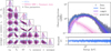 |
Fig. 1 Left: comparison of the posterior distributions obtained from a BXA run with 1k live-points and a MRI run with five rounds and 5k simulations each using summary statistics for a tbabs*(comptt + powerlaw) model. Right: posterior predictive spectra associated with the posterior distribution obtained using summary statistics. The bands detail the (16–84) and (2.5–97.5) percentiles of the posterior predictive spectra. |
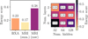 |
Fig. 2 Fig. 2. ES for posterior distributions as produced by BXA, MRI using summary statistics, MRI using raw spectra, and a grid of MRI using a fully connected embedding net with a varying number of layers and hidden parameters. |
4 Feasibility study
The science cases of Athena (Nandra et al. 2013) have evolved through the reformulation of the mission to newAthena (Cruise et al. 2025), in line with the overall performance of the X-IFU, particularly in terms of instrument effective area (mostly related to a change in the mirror collection area). Tailoring observation strategies to constrain relevant physical parameters will require simulating the source in varying parameter regimes to find the best exposure possible. In this section, we demonstrate the feasibility of these studies through SBI with X-IFU for these science cases. The unprecedented spectral resolution of X-IFU motivates the use of sophisticated physical models that allow the emission mechanisms to be described in detail. In this section we investigate the use of SBI to perform this spectral fitting task using a relativistic reflection model, and study how well its parameters can be constrained via the sensitivity of X-IFU, within a given statistical regime (i.e. a given exposure time for a given source flux).
As discussed in Paper I, the amortisation of a NN trained on a single round of simulated spectra is extremely efficient at estimating the posterior distribution for a large set of spectra. This aspect can be used to estimate the ability to measure parameters in a varying range for a given observational set-up, which is extremely useful when designing an observation proposal. This is best done considering SRI, with a test sample for which we can compare the input model parameters with their reconstructed posterior distribution. Ultimately, this will tell us which model parameters X-IFU is able to constrain. Following Barret & Cappi (2019), we are interested in checking what constraints can be derived from X-ray spectroscopy around compact objects, in particular regarding spins; however, we shift our focus here to consider reflection models that are applicable to neutron stars. For this purpose, we took a tbabs*relxillNS model with relxill v2.3.7 (García et al. 2022) and then renormalised the flag set to 1, which relaxes the degeneracy between some parameters. We freed five parameters of the relxillNS model: the dimensionless spin parameter a, the ionisation parameter log ξ, determining the ionisation state of the accretion disk, the reflection fraction, f, which describes the relative strength of reflected emission compared to the direct continuum, and the blackbody temperature kTbb in keV and a normalisation parameter. We generated a target observation of ~3.2M counts (roughly corresponding to a 1 mCrab source observed for 100 ks) and then trained a SRI inference set-up with 200k simulations using the prior specified in Table 1. We trained two inference setups: a SRI set-up fed using the raw spectra and another using summary statistics (defined in Sect. 3.1). Once these set-ups were trained, we were able to infer the posterior distribution from our target observation is seconds. We note that the training process is much slower when compared to MRI set-ups due to the large number of simulations to iterate over. In Fig. 3, we compare the posterior distributions from both set-ups to the reference posterior obtained using BXA with 2k live points. For this high count spectrum, we had to double the number of live points, since using only 1k live points would lead to over-estimated uncertainties. We observe that using summary statistics yield better results overall than working directly with the full spectra, which is consistent with our conclusion in Sect. 3.2.
Once the inference set-up is properly trained, we can use it to generate posterior distributions for new observed spectra, generated with varying parameters around our target observation. Thus, we drew 1000 new parameter values for the spin a, the reflection fraction, f , and the ionisation, log ξ, such that a ~  (0.1,0.3), f ~
  (2.5,4.5), and log ξ ~
  (2,3). Once the posterior distribution was generated for each of these spectra, we were able to compute the accuracy to reconstruct the input parameters using the same ES as that described in Sect. 3.2. In Fig. 4, we plot the value of ES depending on the parameters. We observe no clear trend for a and f, where low and high ES values are distributed uniformly, meaning that the reconstruction is very noisy in the parameter range we chose. On the other hand, log ξ shows a clear trend of low ES for values ~3.2 and high ES for values ~4.4. This can be interpreted as a constraining observation for this parameter in particular, especially for log ξ ε [2.8,3.5]. We clarified this trend by marginalising the reconstructed parameters in the left panel of Fig. 4, where we clearly observe the ability to recover log ξ in a given range, without the capacity to constrain a. We also note that the ES tends to increase slightly bit for very low values of log ξ, which can be attributed to the network poor performances on the boundaries of its training set. The SRI inference set-up are extremely powerful at constraining a lot of spectra at once and can unlock this kind of feasibility studies by quickly constraining portions of the parameter space. Exploring in advance our ability to constrain certain parameters of a model for a given observational set-up will enable us to make the most of the new science that an instrument like X-IFU will be able to produce. We note the generally poorer constraints on the spin parameter, a, when compared to Barret & Cappi (2019). The consideration of a different flavour of the reflection model (relxilllp instead of relxillNS), together with a change in the instrument response, may explain why they obtained tighter constraints on the black hole spin parameter in their study, compared to the poor constraints we get on the neutron star spin parameter. It is clear that within this statistical regime, probing shorter timescales, tighter constraints can still be derived for other parameters (e.g. the ionisation parameter). It is worth adding that multi-layer coatings is currently envisaged for the newAthena optics (to boost the effective area of the mirror around the Iron K line) and this should help to get better constraints on the neutron star spin parameter from reflection spectroscopy.
As an additional discussion, we note that the performance of simulation-based inference in cases of high signal-to-noise ratio is reduced. The normalising flows take advantage of the observation noise to create a mapping between the parameters and the summary statistics that works on average. As with exact approaches, as the signal-to-noise ratio increases, the volume of a posteriori parameter distributions decreases, making it more difficult to produce an exhaustive mapping of this region. Nevertheless, it is possible to couple this feasibility approach with a priori distribution restrictions, as in Paper I. In this situation, for example, the network could be trained more finely to reconstruct spectra between 2 and 4 million counts, thus facilitating constraints on the parameters.
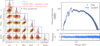 |
Fig. 3 Left: comparison of the posterior distributions obtained from a BXA run with 2 k live-points and SRI run using the whole spectrum or summary stats, trained both with 200k simulations for a tbabs*relxillNS model. Right: posterior predictive spectra associated with the posterior distribution obtained using summary statistics. The bands detail the (16-84) and (2.5-97.5) percentiles of the posterior predictive spectra. |
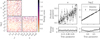 |
Fig. 4 Left: ES obtained from the reconstruction of the spin a, reflection fraction, f , and ionisation, log ξ, for varying values of these parameters in a fixed observational set-up. Right: marginalised constraints for the spin, a, and the ionisation, log ξ, compared to the average ES obtained in each region of the reconstructed parameter space. |
5 Two-temperature plasmas with X-IFU
The ICM can present multiple phases due to dynamical interactions linked, for instance, to the presence of a cool-core or strong feedback from the AGN in the brightest galaxy of the cluster. Probing such spectra can be tricky because of the high degeneracy between the two similar components. In particular, suing SBI with the previous summary statistics, we expect difficulties in assessing the redshift and velocities, which are features encoded in the spectral line position and width. To explore this, we consider a tbabs*(bapec+bapec) model in XSPEC terminology with parameters highlighted in Table 1. The Astrophysical Plasma Emission Code (APEC, Smith et al. 2001) simulates the X-ray emission of an ionised gas, including the continuum mainly dominated by the bremsstrahlung, and emission lines. The parameter kT controls the gas temperature in keV and the abundance Z is linked to the metal content of the gas. A mock observation with a target number of counts of ≃300 k is generated, which corresponds to counts generated by the full field of view of a ~750 s integration in the Perseus core.
As defined in Sect. 3.1, the summary statistics remove the information associated with the spectral lines by diluting them in large energy bins. To overcome this, we added a specific focus on some line complexes, associated with energy bands detailed in Table 2, for which we subdivided the counts in 20 smaller bins. We computed the average energy, Ēi, in each bin, i, weighted by the number of counts:

Here, the summation of j represents the summation of the instrumental channels within the bin, i, and Ej is the mean energy of the channel. This extra statistic can grasp line-related information, such as their shift and broadening, which are directly related to the redshift, z, and velocity, v, parametrised by the bapec model. This is further discussed in Sect. 6.3. Due to a much larger number of summaries, we expect a slower convergence of the neural network. Hence, we fit this spectrum using MRI with 20 rounds of 10k simulations. In Fig. D.2, we display the full posterior distribution compared to a BXA run with 1k live points, along with the posterior predictive spectrum in the [0.5-8] keV band. We observe a good agreement between both posterior distributions, with a more significant spread in the SIXSA reconstructed parameters. As expected, when working with compressed representation for a model with high-frequency features such as emission lines, we lose information on the redshift and velocity, leading to broader distributions for these two parameters. As shown in Fig. 5, we get a satisfactory result for the four line complexes we focussed on during the inference, where the emission lines are well constrained - even if the posterior parameter distribution are not optimal.
We emphasise the necessity of adding emission lines tailored summary statistics in Fig. D.3, where we observe a significant offset and uncertainty on the redshift and velocity parameters when using only summary statistics without focus on the line complex structures. We believe that it is possible to further improve the characterisation of these spectra by investigating summary statistics that better represent this information from the emission lines. Fourier space approaches, wavelet transforms or other methods based on multiscale decomposition such as wavelet scattering transforms (e.g. Andreux et al. 2020) could improve the quality of the results. However, such investigations are beyond the scope of this paper.
Line complexes injected as extra summary statistics for the inference of the tbabs*(bapec+bapec) model.
6 Discussion
6.1 Assessing convergence
At first sight, convergence can be hard to assess for SBI approaches. The question of how many rounds and simulations are needed to get a proper and stable result remains to be addressed. One way to tackle with this challenge is to inspect the training curves of the neural network. In Fig. 6, we display the evolution of the loss evaluated on the training set and validation set. In the first rounds, we observe a rising validation loss compared to a decreasing training loss, which is a signature of early over-fitting. In the first rounds, the training set is too small to let the network learn the full dynamic of the mapping between the parameters, θ, and the observables x. As the number of rounds increases, the total number of simulations and the simulations are closer to the best-fit value, which stabilises the training. Increasing the number of simulations can prevent overfitting, as single round inference is feasible. However, it requires a much larger number of simulations. In general, there is no given rule for stating that a training is over, while the number of epochs and rounds can be considered as another hyperparameter of the network. However, some metrics can offer us some idea about the quality of the training. To check whether the inference set-up converged or not, we can check that the training and validation loss are not improved significantly when running extra inference rounds. We can also check for the stability of the surrogate posterior distributions, which are expected to concentrate towards its most informative state when the number of rounds increases.
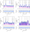 |
Fig. 5 Posterior predictive spectra of the 4 line complexes added as extra summary statistics for a MRI run with a tbabs*(bapec+bapec) model for 20 rounds of 10k simulations: O VIII (a), Fe XXIV + Ne X (b), Fe XXIV + Mg XII (c), and Fe XXV (d). The brightest emission lines are highlighted in each plot. |
6.2 Aiming for the best fit
From the surrogate posterior distributions produced with SBI inference pipelines, we can generate a distribution of posterior log-probability associated with each point, as evaluated in the same standard as BXA. This quantity is directly linked to the well known Cstat such that log P(θ|x) = –Cstat/2. The posterior probability distributions for the 3 problems we treated in this paper are displayed in Fig. 7. For each of these inference problems, we observe that the probability distribution is wider and lower on average compared to BXA, meaning that the surrogate posterior distributions include parameter values that are worse than the one obtained using exact techniques. This translates to either the small offsets or the larger spread that can be observed in the posterior comparisons, such as those given in Figs. 1, 3, and D.2. Using SBI approaches with multi-round inference, we can obtain a fairly good approximation of the best fit, within 10 per cent of the best fit as compared to the results from exact methods. With these approximated distributions, it is hard to directly obtain the best fit per se, but, we can use them to initialise exact methods to increase their efficiency, we can either start a traditional minimisation from the best-fit value obtained using the SBI approach or use the surrogate distributions as proposal distribution for increasing the convergence speed of MCMC methods. Such synergies could improve both the speed and reliability of exact methods, thanks to the fast convergence and robustness of SBI.
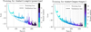 |
Fig. 6 Evolution of the loss for the training and validation set depending on the training epochs and inference round for two spectral models used in this paper. Each round adds a set of 5 k simulations to the global set for the left panel and a set of 10k simulations for the right panel. |
6.3 Understanding the summary statistics
As stated before, the choice of summary statistics for a given problem is not unique and different choices can lead to different posterior distributions. In general, the choice of summary statistics falls under the hyperparameter optimisation and it is not likely to be optimised if a working inference setting is found for a given problem. Instead of defining this set a priori of our problem, we motivated the choice of summaries we performed in this paper a posteriori; in particular, we consider how the addition of the weighted energy in the two components plasma model of Sect. 5 allows us to properly constrain the redshift with spectral line data. To investigate the sensitivity of our summary statistics to a given parameter, we relied on identifying active subspaces, as proposed by Constantine et al. (2014). The active sub-space is aimed at identifying covariant directions in a multivariate function to define a preferred and smaller parameter space. However, we are not interested in finding such a space, but, rather, in identifying the parameters that are sensitive to summary statistics, so we get an interpretable view of what kind of information and constraints they bring. To do so, we first define an arbitrary transformation between the parameter space θ and a given statistic xi . By fitting a lightweight neural network (a two layer ResNet with 100 hidden features, see He et al. 2015) on simulated samples, we obtain a transformation, f , which predicts the expected value of xi given a set of parameters θ. As it can be parametrised using NNs, it is easy to derive and, in particular, we can compute the sensitivity matrix, M, defined as
![Mathematical equation: M = \mathbb{E}_{p(\mathbf{\theta}|x_i)}\left[ (\nabla_{\boldsymbol{\theta}}f). (\nabla_{\boldsymbol{\theta}}f) ^T\right],](/articles/aa/full_html/2025/07/aa55215-25/aa55215-25-eq30.png)
which is the expected value of the outer product of the gradient of f estimated on the posterior distribution support. Here, M is conceptually related to the uncentred covariance of the gradient function and the Fisher information if f is a log-likelihood. The eigenvalues and eigenvector of this sensitivity matrix trace directions of high correlation between the parameters and the investigated summary statistic. Computing the sum of the eigenvectors weighted by the eigenvalues in the parameter space gives the overall preferred direction of the parameters for this given summary statistics, which we refer to as the sensitivity.
We applied this method to the double plasma model from Sect. 5, investigating the link between the statistics and the model parameters. We used standard normalised parameters to facilitate the training of f for each statistic. We reduced the sums, hardness ratios, differential ratios, and weighted energies by taking the maximum sensitivity for each band considered. The resulting sensitivity is further normalised to get comparable quantities for each summary statistics. The corresponding sensitivities are displayed in Fig. 8. From this figure, we can understand how each summary helps us in constraining a specific parameter. For instance, global quantities such as the mean, sum and standard deviation are mostly sensitive to the normalisation of both components, while statistics computed in bins such as the sum, hardness ratios and differential ratios trace the shape of the spectrum with their high correlation to the temperature. Finally, the weighted energy computed in complexes informs about the redshift and velocity. As shown in Fig. 5, the first component dominates the first three complexes, showing good correlation of the redshift z1 for the second and third. On the other hand, the last complex is dominated by the second component, which shows good correlation for both z2 and v2. The increasing sensitivity to the velocity with the complex number can point to its increased effect with energy, as the induced broadening scales as σ ∝ vE. Such an analysis further highlights the need for additional statistics to constrain the line-related information in this model and brings interpretability to the SBI approach with physically motivated compression, unlike a principal component analysis. It also illustrates how incorporating specific domain knowledge is key in improving the performance of ML approaches.
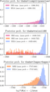 |
Fig. 7 Comparison of the distribution of posterior probability for the samples produced using BXA and the various SBI inference pipelines used in this paper. |
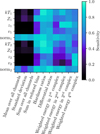 |
Fig. 8 Sensitivity of each summary statistics to the parameters of a tbabs*(bapec+bapec). The sensitivity arrays are normalised to allow qualitative comparison between the summary statistics. |
7 Conclusions
In this paper, we demonstrate the feasibility of simulation-based inference for high-resolution X-ray spectroscopy. Simulationbased inference relies on neural networks learning probability density transformations between the parameter space and the simulated observables, without requiring an explicit formulation of the likelihood for the problem. Thus, it can be used to obtain well-defined posterior distributions for the parameters. In contrast to our previous work, we focus here on high-energy resolution spectra, such as those produced by newAthena/X-IFU. The key to using SBI approaches for high-resolution spectroscopy is spectral compression using summary statistics, which reduces the 24k channel spectra to a hundred or so values that encapsulate their spectral features. We show that this approach allows us to recover the parameters of multi-component models, as well as exact computations using nested sampling, while drastically reducing inference time and the number of likelihood evaluations required. We also explore the use of embedding networks to automatically learn compression schemes, however, they demonstrate a poor performance compared to hand-crafted summary statistics. Single-round inference requires many simulations to train an amortised network, but once trained, it can infer parameter values almost instantaneously. It can be used to fit many spectra and, for example, to explore the constrainable parameter values for a given observation proposal. Multiple-round inference can only fit a single spectrum, but it provides well-calibrated posterior distributions with significantly less computational effort and time compared to exact methods. The use of summary statistics on top of these two approaches increases the interpretability of this machine learning approach, as specific features such as emission lines require specific summary statistics that are physically motivated. We believe that SBI has great potential for the next decades of high-energy astrophysics, as it drastically reduces the computational requirements while still being close to achieving an exact inference. Finding efficient compression schemes is the key to improving this approach and fully exploiting the vast store of data offered by the upcoming generation of high-resolution X-ray spectrometers.
Acknowledgements
S.D. & D.B. would like to thank all their colleagues, in particular Fabio Acero, Alexei Molin, Etienne Pointecouteau for their support and encouragement in developing further the power of SBI-NPE. Special thanks to Jonas Gérard and Yannis Guillelmet for contributing to the testing of the sbi toolkit. We also thank Thomas Dauser for support in implementing and testing extensively the relxill package, whose models are part of the most challenging ones tested here. In addition to the sbi package (Tejero-Cantero et al. 2020), this work made use of many awesome Python packages: ChainConsumer (Hinton 2016), matplotlib (Hunter 2007), numpy (Harris et al. 2020), pandas (McKinney 2010), pytorch (Paszke et al. 2017), scikit-learn (Pedregosa et al. 2011), scypi (Virtanen et al. 2020), tensorflow (Abadi et al. 2015).
Appendix A Including background
Including a background spectrum in the inference using SBI is straightforward. If an independent spectrum containing a background realisation is available, and if a motivated model exists for it, it is only necessary to add another spectral component to the spectral model, which is fitted to the background spectrum and the source+background spectrum, in addition to the source spectral model. However, in this section we chose to focus on the capability of SBI to perform an automatic marginalisation over the nuisance parameters. If we have an independent realisation of the background, we can add a Poisson realisation of it to the modelled source spectrum during the simulation process. Accounting for such an effect in a traditional likelihood framework would require to perform marginalisation over the background parameters, thus involving numerical integration over each bin of the spectrum. Using SBI, this is straightforward to implement and requires almost no computational overhead.
We demonstrate this using a similar observational set-up as in Sect. 3.1, considering the case where a background spectrum is provided independently. We generate two background spectra, one to be added to the source spectrum and another independent realisation that we consider as our observed background. Inference is performed on the source+background spectrum. The background is simulated using a tbabs*powerlaw model parameterised to contribute ~10% of the total counts of the source+background spectrum. The results are compared to a BXA run with 1k livepoints with cstat minimisation, and the posterior parameters are displayed in Fig. A.1, where we observe a good agreement between the two approaches, while remaining orders of magnitude faster to compute.
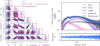 |
Fig. A.1 Left: Comparison of the posterior distributions obtained from a BXA run with 1k live-points and a MRI run with five rounds and 5k simulations each using summary statistics for a tbabs*(comptt + powerlaw) model, with the inclusion of a background spectrum. Right: Posterior predictive spectra associated with the posterior distribution obtained using summary statistics. The bands detail the (16-84) and (2.5-97.5) percentiles of the posterior predictive spectra. |
Appendix B Question of whether or not to prune
We show in this paper that the regularisation of the observables using compression schemes such as summary statistics is a key feature in improving the efficiency of the SBI approach. In particular, the centrality of the observable in the training set induced by the summary statistics increases the training efficiency. In this sense, it is easy to prune summary statistics that do not cover the spectrum statistics. This is expected to increase both the speed and quality of training, as we work with fewer and more representative statistics. However, when pruning in a multi-round scheme, as the simulations get closer to the observable after each round, some statistics become relevant again, while others should be discarded. In this situation, we have to retrain the network from scratch in each round, as the nature of the observable changes. In addition, we cannot train on the previously generated simulations, as they are no longer relevant. So when pruning, we have to consider this trade-off between speed and efficiency. Figure B.1 shows how the training and validation losses evolve when the network is retrained from scratch. This demonstrates the network ability to converge in a small number of epochs, thanks to the proposal distribution generating a training sample that is closer to the true posterior distribution with each iteration.
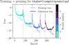 |
Fig. B.1 Evolution of the loss for the training and validation set depending on the training epochs and inference round for the tbabs*(comptt+powerlaw), with an extra-pruning of the marginal summary statistics at each round and retraining from scratch. |
Appendix C Application to true spectra
To assess the applicability of summary statistics to real observational data, we apply our methodology to the same ULX spectrum used as a reference in Dupourqué et al. (2024). This dataset corresponds to an XMM-Newton observation of NGC 7793 ULX-4, previously reduced and analysed by Quintin et al. (2021), and features a high-quality EPIC-PN spectrum with no background subtraction. The source emission is well described by an absorbed dual-component model (tbabs*(powerlaw+blackbodyrad)), typical for ULXs exhibiting both thermal and non-thermal components. Using the same inference set-up as in the previous work, we apply both BXA and a MRI approach with five rounds of 5,000 simulations each. The posterior predictive and comparison of posterior distributions are shown in Fig. C.1, further validating the robustness of summary statistics on real astrophysical data.
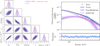 |
Fig. C.1 Left: Comparison of the posterior distributions obtained from a BXA run with 1k live-points and MRI run using summary stats for the spectrum of NGC 7793 ULX-4. Right: Posterior predictive spectra associated with the posterior distribution obtained using summary statistics. The bands detail the (16-84) and (2.5-97.5) percentiles of the posterior predictive spectra. |
Appendix D Extra figures
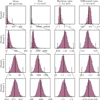 |
Fig. D.1 Evolution of the mean value of the spectrum, the sum, hardness ratio and differential ratios around 0.5 keV in the tbabs*(comptt+powerlaw) model. The true value is displayed in a black vertical line. |
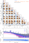 |
Fig. D.2 Top: Comparison of the posterior distributions obtained from a BXA run with 1k live-points and MRI run using summary stats tbabs*(bapec+bapec) model for 20 rounds of 10k simulations. Bottom: Posterior predictive spectra associated with the posterior distribution obtained using summary statistics and focus on 4 line complexes. The bands detail the (16-84) and (2.5-97.5) percentiles of the posterior predictive spectra. |
 |
Fig. D.3 Comparison of the posterior marginal distributions obtained from a BXA run with 1k live-points, MRI run using summary stats and extra weighted energies from complexes tbabs*(bapec+bapec) model for 20 rounds of 10k simulations and MRI in the same set-up with only summary stats. |
References
- Abadi, M., Agarwal, A., Barham, P., et al. 2015, TensorFlow: Large-Scale Machine Learning on Heterogeneous Systems, software available from tensorflow.org [Google Scholar]
- Andreux, M., Angles, T., Exarchakis, G., et al. 2020, J. Mach. Learn. Res., 21, 1 [Google Scholar]
- Arnaud, K. A. 1996, ASP Conf. Ser., 101, 17 [Google Scholar]
- Ayesha, S., Hanif, M. K., & Talib, R. 2020, Information Fusion, 59, 44 [Google Scholar]
- Barret, D., & Cappi, M. 2019, A&A, 628, A5 [NASA ADS] [CrossRef] [EDP Sciences] [Google Scholar]
- Barret, D., & Dupourqué, S. 2024, A&A, 686, A133 [NASA ADS] [CrossRef] [EDP Sciences] [Google Scholar]
- Barret, D., Albouys, V., Herder, J.-W. d., et al. 2023, Exp. Astron., 55, 373 [NASA ADS] [CrossRef] [Google Scholar]
- Betancourt, M. J., & Girolami, M. 2013, Hamiltonian Monte Carlo for Hierarchical Models (Chapman and Hall: CRC Press) [Google Scholar]
- Bonson, K., & Gallo, L. C. 2016, MNRAS, 458, 1927 [NASA ADS] [CrossRef] [Google Scholar]
- Buchner, J., & Boorman, P. 2024, Statistical Aspects of X-ray Spectral Analysis, eds. C. Bambi, & A. Santangelo (Singapore: Springer Nature Singapore), 5403 [Google Scholar]
- Buchner, J., Georgakakis, A., Nandra, K., et al. 2014, A&A, 564, A125 [NASA ADS] [CrossRef] [EDP Sciences] [Google Scholar]
- Cash, W. 1979, ApJ, 228, 939 [Google Scholar]
- Choudhury, K., Garcia, J. A., Steiner, J. F., & Bambi, C. 2017, ApJ, 851, 57 [NASA ADS] [CrossRef] [Google Scholar]
- Constantine, P. G., Dow, E., & Wang, Q. 2014, SIAM J. Sci. Comput., 36, A1500 [Google Scholar]
- Cruise, M., Guainazzi, M., Aird, J., et al. 2025, Nat. Astron., 9, 36 [Google Scholar]
- de Plaa, J., Kaastra, J. S., Gu, L., Mao, J., & Raassen, T. 2019, SPEX: HighResolution Spectral Modeling and Fitting for X-ray Astronomy (Boston: ASP) [Google Scholar]
- Deistler, M., Macke, J. H., & Gonçalves, P. J. 2022, Proc. Natl. Acad. Sci., 119, e2207632119 [NASA ADS] [CrossRef] [Google Scholar]
- Dupourqué, S., Barret, D., Diez, C. M., Guillot, S., & Quintin, E. 2024, A&A, 690, A317 [NASA ADS] [CrossRef] [EDP Sciences] [Google Scholar]
- García, J. A., Dauser, T., Ludlam, R., et al. 2022, ApJ, 926, 13 [CrossRef] [Google Scholar]
- Gneiting, T., & Raftery, A. E. 2007, J. Am. Stat. Assoc., 102, 359 [CrossRef] [Google Scholar]
- Greenberg, D. S., Nonnenmacher, M., & Macke, J. H. 2019, arXiv e-prints [arXiv:1905.07488] [Google Scholar]
- Harris, C. R., Millman, K. J., van der Walt, S. J., et al. 2020, Nature, 585, 357 [NASA ADS] [CrossRef] [Google Scholar]
- Hastings, W. K. 1970, Biometrika, 57, 97 [Google Scholar]
- He, K., Zhang, X., Ren, S., & Sun, J. 2015, Deep Residual Learning for Image Recognition (California: IEEE) [Google Scholar]
- Hinton, S. R. 2016, J. Open Source Softw., 1, 00045 [NASA ADS] [CrossRef] [Google Scholar]
- Houck, J. C., & Denicola, L. A. 2000, ASP Conf. Ser., 216, 591 [Google Scholar]
- Hunter, J. D. 2007, Comput. Sci. Eng., 9, 90 [NASA ADS] [CrossRef] [Google Scholar]
- Ichinohe, Y., Yamada, S., Miyazaki, N., & Saito, S. 2018, MNRAS, 475, 4739 [NASA ADS] [CrossRef] [Google Scholar]
- Jimenez Rezende, D., & Mohamed, S. 2016, arXiv e-prints [arXiv:1505.05770] [Google Scholar]
- Kaastra, & Bleeker. 2016, Antike und Abendland, 587, A151 [Google Scholar]
- Kingma, D. P., & Ba, J. 2017, arXiv e-prints [arXiv:1412.6980] [Google Scholar]
- McKinney, W. 2010, in Proceedings of the 9th Python in Science Conference, eds. S. van der Walt, & J. Millman, 51 [Google Scholar]
- Nandra, K., Barret, D., Barcons, X., et al. 2013, arXiv e-prints [arXiv:1306.2307] [Google Scholar]
- Papamakarios, G., Pavlakou, T., & Murray, I. 2017, in Advances in Neural Information Processing Systems (UK: Curran Associates, Inc.), 30 [Google Scholar]
- Parker, M. L., Lieu, M., & Matzeu, G. A. 2022, MNRAS, 514, 4061 [NASA ADS] [CrossRef] [Google Scholar]
- Paszke, A., Gross, S., Chintala, S., et al. 2017, in NIPS Autodiff Workshop [Google Scholar]
- Pedregosa, F., Varoquaux, G., Gramfort, A., et al. 2011, J. Mach. Learn. Res., 12, 2825 [Google Scholar]
- Peille, P., Barret, D., Cucchetti, E., et al. 2025, Exp. Astron., 59, 18 [Google Scholar]
- Quintin, E., Webb, N. A., Gérpide, A., Bachetti, M., & Fürst, F. 2021, MNRAS, 503, 5485 [NASA ADS] [CrossRef] [Google Scholar]
- Siemiginowska, A., Burke, D., Günther, H. M., et al. 2024, ApJS, 274, 43 [Google Scholar]
- Skilling, J. 2006, Bayesian Analysis, 1, 833 [CrossRef] [Google Scholar]
- Smith, R. K., Brickhouse, N. S., Liedahl, D. A., & Raymond, J. C. 2001, ApJ, 556, L91 [Google Scholar]
- Tejero-Cantero, A., Boelts, J., Deistler, M., et al. 2020, J Open Source Softw., 5, 2505 [Google Scholar]
- Titarchuk, L. 1994, ApJ, 434, 570 [NASA ADS] [CrossRef] [Google Scholar]
- Tutone, A., Anitra, A., Ambrosi, E., et al. 2025, A&A, 696, A77 [NASA ADS] [CrossRef] [EDP Sciences] [Google Scholar]
- Virtanen, P., Gommers, R., Oliphant, T. E., et al. 2020, Nat. Methods, 17, 261 [Google Scholar]
- XRISM Science Team 2020, Science with the X-ray Imaging and Spectroscopy Mission (XRISM) (USA: NASA) [Google Scholar]
- Zanetta, F., & Allen, S. 2024, Scoringrules: a python library for probabilistic forecast evaluation, https://github.com/frazane/scoringrules [Google Scholar]
Note: in this paper we have not covered the case where the spectra follow an effective Gaussian statistic, as provided by some reduction software. This could be achieved by simply switching from a Poisson realisation to a Gaussian realisation with the associated (co-)variance.
All Tables
Parameters true value and prior distribution used in the three models described in this paper.
Line complexes injected as extra summary statistics for the inference of the tbabs*(bapec+bapec) model.
All Figures
|
Fig. 1 Left: comparison of the posterior distributions obtained from a BXA run with 1k live-points and a MRI run with five rounds and 5k simulations each using summary statistics for a tbabs*(comptt + powerlaw) model. Right: posterior predictive spectra associated with the posterior distribution obtained using summary statistics. The bands detail the (16–84) and (2.5–97.5) percentiles of the posterior predictive spectra. |
| In the text | |
|
Fig. 2 Fig. 2. ES for posterior distributions as produced by BXA, MRI using summary statistics, MRI using raw spectra, and a grid of MRI using a fully connected embedding net with a varying number of layers and hidden parameters. |
| In the text | |
|
Fig. 3 Left: comparison of the posterior distributions obtained from a BXA run with 2 k live-points and SRI run using the whole spectrum or summary stats, trained both with 200k simulations for a tbabs*relxillNS model. Right: posterior predictive spectra associated with the posterior distribution obtained using summary statistics. The bands detail the (16-84) and (2.5-97.5) percentiles of the posterior predictive spectra. |
| In the text | |
|
Fig. 4 Left: ES obtained from the reconstruction of the spin a, reflection fraction, f , and ionisation, log ξ, for varying values of these parameters in a fixed observational set-up. Right: marginalised constraints for the spin, a, and the ionisation, log ξ, compared to the average ES obtained in each region of the reconstructed parameter space. |
| In the text | |
|
Fig. 5 Posterior predictive spectra of the 4 line complexes added as extra summary statistics for a MRI run with a tbabs*(bapec+bapec) model for 20 rounds of 10k simulations: O VIII (a), Fe XXIV + Ne X (b), Fe XXIV + Mg XII (c), and Fe XXV (d). The brightest emission lines are highlighted in each plot. |
| In the text | |
|
Fig. 6 Evolution of the loss for the training and validation set depending on the training epochs and inference round for two spectral models used in this paper. Each round adds a set of 5 k simulations to the global set for the left panel and a set of 10k simulations for the right panel. |
| In the text | |
|
Fig. 7 Comparison of the distribution of posterior probability for the samples produced using BXA and the various SBI inference pipelines used in this paper. |
| In the text | |
|
Fig. 8 Sensitivity of each summary statistics to the parameters of a tbabs*(bapec+bapec). The sensitivity arrays are normalised to allow qualitative comparison between the summary statistics. |
| In the text | |
|
Fig. A.1 Left: Comparison of the posterior distributions obtained from a BXA run with 1k live-points and a MRI run with five rounds and 5k simulations each using summary statistics for a tbabs*(comptt + powerlaw) model, with the inclusion of a background spectrum. Right: Posterior predictive spectra associated with the posterior distribution obtained using summary statistics. The bands detail the (16-84) and (2.5-97.5) percentiles of the posterior predictive spectra. |
| In the text | |
|
Fig. B.1 Evolution of the loss for the training and validation set depending on the training epochs and inference round for the tbabs*(comptt+powerlaw), with an extra-pruning of the marginal summary statistics at each round and retraining from scratch. |
| In the text | |
|
Fig. C.1 Left: Comparison of the posterior distributions obtained from a BXA run with 1k live-points and MRI run using summary stats for the spectrum of NGC 7793 ULX-4. Right: Posterior predictive spectra associated with the posterior distribution obtained using summary statistics. The bands detail the (16-84) and (2.5-97.5) percentiles of the posterior predictive spectra. |
| In the text | |
|
Fig. D.1 Evolution of the mean value of the spectrum, the sum, hardness ratio and differential ratios around 0.5 keV in the tbabs*(comptt+powerlaw) model. The true value is displayed in a black vertical line. |
| In the text | |
|
Fig. D.2 Top: Comparison of the posterior distributions obtained from a BXA run with 1k live-points and MRI run using summary stats tbabs*(bapec+bapec) model for 20 rounds of 10k simulations. Bottom: Posterior predictive spectra associated with the posterior distribution obtained using summary statistics and focus on 4 line complexes. The bands detail the (16-84) and (2.5-97.5) percentiles of the posterior predictive spectra. |
| In the text | |
|
Fig. D.3 Comparison of the posterior marginal distributions obtained from a BXA run with 1k live-points, MRI run using summary stats and extra weighted energies from complexes tbabs*(bapec+bapec) model for 20 rounds of 10k simulations and MRI in the same set-up with only summary stats. |
| In the text | |
Current usage metrics show cumulative count of Article Views (full-text article views including HTML views, PDF and ePub downloads, according to the available data) and Abstracts Views on Vision4Press platform.
Data correspond to usage on the plateform after 2015. The current usage metrics is available 48-96 hours after online publication and is updated daily on week days.
Initial download of the metrics may take a while.