| Issue |
A&A
Volume 696, April 2025
|
|
|---|---|---|
| Article Number | A77 | |
| Number of page(s) | 11 | |
| Section | Numerical methods and codes | |
| DOI | https://doi.org/10.1051/0004-6361/202553690 | |
| Published online | 04 April 2025 | |
X-ray spectral fitting with Monte Carlo dropout neural networks
1
Istituto Nazionale di Astrofisica INAF IASF Palermo,
Via Ugo La Malfa 153,
Palermo
90146, Italy
2
ICSC – Centro Nazionale di Ricerca in HPC, Big Data e Quantum Computing,
Italy
3
Dipartimento di Fisica, Università degli Studi di Cagliari,
SP Monserrato-Sestu, KM 0.7,
Monserrato,
09042
Italy
4
Dipartimento di Fisica e Chimica – Emilio Segrè, Università di Palermo,
via Archirafi 36,
90123
Palermo, Italy
5
INAF – Osservatorio Astronomico di Roma,
Via Frascati 33,
00076
Monte Porzio Catone (RM), Italy
6
Istituto Nazionale di Fisica Nucleare Sezione di Catania,
Via Santa Sofia 64,
95123
Catania, Italy
★ Corresponding author; This email address is being protected from spambots. You need JavaScript enabled to view it.
Received:
7
January
2025
Accepted:
10
March
2025
Abstract
Context. The analysis of X-ray spectra often encounters challenges due to the tendency of frequentist approaches to be trapped in local minima, affecting the accuracy of spectral parameter estimation. Bayesian methods offer a solution to this issue, though computational time significantly increases, limiting their scalability. In this context, neural networks have emerged as a powerful tool for efficiently addressing these challenges, providing a balance between accuracy and computational efficiency.
Aims. This work aims to explore the potential of neural networks to recover model parameters and quantify their uncertainties. We benchmark their accuracy and computational time performance against traditional X-ray spectral fitting methods based on frequentist and Bayesian approaches. This study serves as a proof of concept for data analysis of future astronomical missions, producing extensive datasets that could benefit from the proposed methodology.
Methods. We applied Monte Carlo dropout to a range of neural network architectures to analyze X-ray spectra. Our networks are trained on simulated spectra derived from a multiparameter source emission model convolved with an instrument response. This allows them to learn the relationship between the spectra and their corresponding parameters while generating posterior distributions. The model parameters are drawn from a predefined prior distribution. To illustrate the method, we used data simulated with the response matrix of the X-ray instrument NICER. We focus on simple X-ray emission models with up to five spectral parameters for this proof of concept.
Results. Our approach delivers well-defined posterior distributions, comparable to those produced by Bayesian inference analysis, while achieving an accuracy similar to traditional spectral fitting. It is significantly less prone to falling into local minima, thus reducing the risk of selecting parameter outliers. Moreover, this method substantially improves computational speed compared to other Bayesian approaches, with computational time reduced by roughly an order of magnitude.
Conclusions. Our method offers a robust alternative to the traditional spectral fitting procedures. Despite some remaining challenges, this approach can potentially be a valuable tool in X-ray spectral analysis, providing fast, reliable, and interpretable results with reduced risk of convergence to local minima, effectively scaling with data volume.
Key words: methods: data analysis / methods: statistical / X-rays: binaries
© The Authors 2025
 Open Access article, published by EDP Sciences, under the terms of the Creative Commons Attribution License (https://creativecommons.org/licenses/by/4.0), which permits unrestricted use, distribution, and reproduction in any medium, provided the original work is properly cited.
This article is published in open access under the Subscribe to Open model. This email address is being protected from spambots. You need JavaScript enabled to view it. to support open access publication.
1 Introduction
The analysis of X-ray spectra has been essential to revealing the physical characteristics of astrophysical objects like active galactic nuclei, accreting neutron stars, and black hole binaries. Traditionally, spectral fitting, in which physically motivated model parameters are adjusted to match observed data, has been the primary method used in this domain. In recent years, approaches based on both frequentist and Bayesian statistics have proven to be effective, allowing researchers to infer best-fitting model parameters through the use of software such as XSPEC (Arnaud 1996), SPEX (Kaastra et al. 1996), and BXA (Buchner et al. 2014). However, these tools can be computationally demanding, especially as astronomical datasets expand with current missions like XRISM (X-Ray Imaging and Spectroscopy Mission) and eROSITA (extended ROentgen Survey with an Imaging Telescope Array) (Tashiro et al. 2018; Predehl et al. 2021) and future missions such as NewAthena (Barret et al. 2023), where both the volume of data and the increase in features from higher spectral resolution will significantly impact data analysis.
Recent advances in machine learning, artificial intelligence that enables computers to learn from data and improve their performance on tasks without being explicitly programmed, have introduced new approaches to X-ray spectral analysis. For example, Tzavellas et al. (2024) and Bégué et al. (2024) trained neural networks (NNs) to generate spectra from physical parameters, enabling rapid model simulations. Another approach uses NNs to estimate model parameters directly from the observed spectra, bypassing the need for traditional iterative fitting (Ichinohe et al. 2018; Parker et al. 2022; Barret & Dupourqué 2024). Both methods significantly improve speed and efficiency depending on whether the goal is to generate spectra or extract parameters. However, a major challenge remains in obtaining robust uncertainty quantification, which is crucial for reliable astrophysical inferences. Additionally, many existing methods depend on restrictive preprocessing steps, such as narrowing parameter priors or applying dimensionality reduction techniques. While these steps can improve performance, they often limit the flexibility and generalizability of the models, reducing their applicability to diverse datasets.
Our study builds upon these recent advances by applying Monte Carlo dropout (MCD; Gal & Ghahramani 2015), a technique for approximating Bayesian inference through NNs, to X-ray spectral fitting. This approach provides a robust framework for parameter estimation, including uncertainty quantification, comparable to traditional Bayesian methods but with improved computational efficiency. We trained NNs using simulated spectra generated from multiparameter emission models convolved with the instrument response of the NICER (Neutron Star Interior Composition ExploreR) X-ray observatory (Gendreau et al. 2012), which operates in the 0.2–12 keV energy range. The models used to simulate the training dataset are relatively simple, involving up to five parameters, an approach commonly employed in recent studies (Parker et al. 2022; Barret & Dupourqué 2024).
The goal of this work is to demonstrate that NNs, combined with MCD, can reliably recover model parameters and their uncertainties from X-ray spectra. Our method is benchmarked against standard spectral fitting techniques and shows significant improvements in computational speed, allowing for real-time data analysis. By doing so, we lay the groundwork for applying these methods to future astronomical missions, such as NewAthena, which will produce vast and complex datasets that traditional methods may struggle to handle efficiently. Furthermore, this approach proves particularly useful for survey analysis, where the ability to process large volumes of data quickly and accurately is essential. The use of NNs in spectral analysis offers speed and a reduction in the risk of local minima trapping, a common issue for conventional fitting algorithms.
In Sect. 2, we present the methods used to generate the training datasets (Sect. 2.1), construct the neural network (Sect. 2.2), and evaluate the model performance on simulated data (Sect. 2.3). In Sect. 3, we apply our approach to real observational data, demonstrating its effectiveness in practical scenarios. Finally, in Sect. 4 we discuss the implications of our findings, highlight the advantages and limitations of our method, and propose potential avenues for future work.
2 Methods
The fundamental steps of our methodology are as follows:
We began by generating an extensive dataset of simulated X-ray spectra.
We then trained the NN using the generated datasets.
Finally, we evaluated the model’s performance.
Detailed explanations of each step are provided in the next sections.
2.1 Dataset generation
We used PYXSPEC (Gordon & Arnaud 2021), the PYTHON wrapper for XSPEC, to simulate the dataset of spectra for the NN training. We computed the dataset following Barret & Dupourqué (2024), whose recent and detailed work we adopted as a benchmark to facilitate comparison among different NN-based methods. By aligning with their approach, we ensure consistency in dataset structure and simulation strategies, enabling a more direct evaluation of the performance of various NN models.
Initially, we adopted a simple model (Model A) consisting of a powerlaw continuum emission multiplied by the Tübingen-Boulder model for the absorption by the interstellar medium (ISM), tbabs in XSPEC. We set the most updated ISM abundances and cross sections (Wilms et al. 2000; Verner et al. 1996). For the simulations, we used the NICER response file ni1050300108mpu7, corresponding to observation 1050300108 in the NICER archive (see Sect. 3). The simulated spectra were re-binned with five consecutive channels per bin, resulting in ~140 bins per spectrum, covering the energy range from 0.3 to 10 keV. The range of the simulated parameters, for the Model A configuration, is specified in Table 1. The parameters were randomly sampled within the specified ranges, avoiding using a grid search approach. We assumed uniform distributions in linear space for the interstellar equivalent absorption column, NH , the Photon Index of the power law component, and a logarithmic distribution for its normalization. We used the fakeit command in XSPEC to generate the synthetic spectra.
Following the approach of Barret & Dupourqué (2024), we began by selecting a set of parameter values from Model A to define a reference model: NH = 0.2 × 1022 cm−2, Photon Index = 1.7, and NormPL = 1 photons/(keV cm2 s) at 1 keV. Using these parameters, we simulated two reference spectra with different exposure times: 1 second and 10 seconds, corresponding to approximately 2 × 10³ and 2 × 10⁴ total counts, respectively.
Using these reference spectra as a baseline, we generated two distinct datasets. We simulated 104 spectra for each exposure time by varying the model parameters within the ranges specified in Table 1 while keeping the exposure time fixed to 1 second or 10 seconds. These datasets are referred to as “Dataset-short” (for 1-second exposure) and “Dataset-long” (for 10-second exposure). This approach captures realistic spectral variability typical of different classes of X-ray emitting sources while also reflecting the distinct signal-to-noise regimes associated with different exposure times.
In Fig. 1, we present the distribution of the total counts for the spectra in our two datasets, Dataset-short and Dataset- long, respectively. Unlike in Barret & Dupourqué (2024), our datasets show some overlap in total counts. This difference arises because Barret & Dupourqué (2024) initially narrows the parameter range around the reference spectrum. Specifically, they use a ResNet classifier (He et al. 2016) to quickly approximate the values of the parameters, effectively reducing the parameter search space before the main analysis. Alternatively, they performed a coarse inference, in which the network is trained with limited samples. The posterior conditioned on the reference observation is then used as a restricted prior for subsequent analysis. While these methods are powerful and effective, as demonstrated in their work, our focus is on evaluating the predictive power of our NN and its ability to estimate uncertainties. By avoiding parameter range narrowing techniques, we aim to maintain the generality of our model after training, making it more versatile for a broader range of scenarios. As in Barret & Dupourqué (2024), we opted not to include any instrumental background in our simulations. Nonetheless, if an analytical model for the background were available, the network could be trained to account for both the source and background spectra by expanding the number of model parameters. This approach, however, would necessitate a larger training dataset, which could, in turn, lead to longer inference times.
As is common practice in NN applications (Bishop 1995; Goodfellow et al. 2016), both the input spectra and the output parameters are preprocessed before being fed into the network to improve the effectiveness of the training process. Our tests showed that input normalization plays a fundamental role in stabilizing the optimization process, while the parameter normalization mainly helps in balancing the predictive accuracy across different parameters. We used the scikit-learn package (Pedregosa et al. 2011) for this task. Specifically, we standardized the input spectra by applying the StandardScaler to each energy bin independently, adjusting the values so that each bin across all spectra has a mean of zero and a variance of one. This step was necessary to prevent high-count regions from dominating the optimization and to ensure that all spectral features contribute effectively to the learning process. Additionally, by bringing all spectra onto a similar scale, this normalization helps prevent numerical instabilities that could cause the training process to diverge rather than to converge.
We applied normalization for the output parameters, which rescales the values to fit within the [0, 1] range using the MinMaxScaler. Our tests indicated that this step helped ensure that all parameters were treated with comparable importance by the network. Without this rescale, parameters with large numerical values tended to have a stronger influence on the optimization, potentially leading to imbalances in predictive accuracy. Such an approach improved the consistency of the model’s predictions by bringing all parameters onto the same scale.
Each dataset is then divided into three subsets: 60% of the data is used for training the network, 20% is reserved for validation, which is used to tune the model and prevent overfitting, and the remaining 20% is set aside for testing, allowing us to evaluate the final performance of the trained model on unseen data.
Parameter ranges for Model A, defined according to the XSPEC convention.
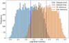 |
Fig. 1 Distribution of total counts for the spectra in the two datasets. The blue histogram represents the dataset based on the reference spectrum with approximately 2 × 10³ total counts (Dataset-short). In comparison, the orange histogram corresponds to the dataset based on the reference spectrum with approximately 2 × 10⁴ total counts (Dataset- long). Both distributions illustrate the variability in total counts due to the range of parameters used in the simulations. Vertical dashed lines show the position of the two reference spectra. |
2.2 Training of the networks
Predicting continuous-valued physical parameters is a classical statistical regression problem. To address it, we explored three different NN architectures: an artificial neural network (ANN), a convolutional neural network (CNN) combined with an ANN (CNN+ANN), and a gated recurrent unit (GRU)-based architecture. Below, we briefly describe these architectures and their relevance for this task:
ANNs are the fundamental type of NN, consisting of multiple layers of neurons interconnected through learnable weights. Each neuron performs a weighted sum of its inputs, followed by a nonlinear activation function. ANNs are highly versatile and can approximate complex nonlinear relationships, making them suitable for basic regression tasks (Bishop 1995).
CNNs are designed to automatically and adaptively learn spatial hierarchies of features from input data through a series of convolutional layers (Lecun et al. 1998). The CNN+ANN combination starts with convolutional layers that capture local patterns in the spectral data, which are then flattened and passed to a dense ANN structure to map these features to the final output. This architecture leverages local feature extraction and global pattern recognition, enhancing performance when input data have spatial or temporal dependences.
A GRU is a type of recurrent neural network (RNN) designed to handle sequential data by maintaining hidden states over time steps (Cho et al. 2014). This property allows GRUs to capture temporal dependences and contextual information in the spectral data, which can be crucial for identifying correlations between spectral bins. GRUs are a simplified version of long short-term memory networks; they provide similar performance but with a lower computational cost, making them a particularly suitable tool in cases of limited computational resources.
To effectively capture uncertainties in our predictions, we used MCD (Gal & Ghahramani 2015), a technique that extends traditional dropout to approximate Bayesian inference in NNs. Dropout is typically employed as a regularization method during training, where a fraction of neurons in each layer is randomly deactivated to prevent overfitting (Srivastava et al. 2014). In our approach, however, dropout remains active during inference, enabling the model to generate a range of predictions for each input. This method effectively turns the network into a probabilistic model by simulating posterior sampling. Specifically, when performing inference with dropout enabled, the network generates slightly different predictions for the same input each time, as different subsets of neurons are activated on each forward pass. These varying predictions can then approximate a posterior distribution on the model’s output, enabling the NN to behave like a probabilistic model.
We refer to this approach as MonteXrist (Monte Carlo X-Ray Inference with Spectral Training), leveraging MCD to produce posterior distributions for model parameters. MonteXrist thus provides a robust framework for parameter estimation and uncertainty quantification, with the network generating a distribution of possible outputs that reflects the posterior distribution of model parameters. This probabilistic output enables more reliable predictions by representing the inherent uncertainty in the dataset.
For the training, we used the TensorFlow and Keras frameworks (Abadi et al. 2015; Chollet et al. 2015). In NNs, certain settings, known as hyperparameters, need to be chosen in advance to define the network’s structure and how it learns. These include aspects such as the number of hidden layers, which are layers of neurons that process data and learn patterns within it, and the number of neurons in each layer, which affects the level of detail the network can capture. More layers and more neurons allow the network to model more complex relationships, but they also increase the computational requirements and the risk of overfitting, namely when the model becomes too specialized in the training data and performance worsens with new data. Another key hyperparameter is the learning rate, which controls how quickly the model updates its parameters as it learns from data. A higher learning rate makes the model adjust faster but can lead to instability, while a lower rate makes learning slower but often more precise. We also set the batch size, which is the number of samples the network processes at a time before updating its parameters; this choice influences both the speed and stability of learning. The architecture of the network, including the arrangement of GRU (or ANN) layers, dropout layers, and the layer used for output regression, is illustrated in Fig. 2.
Due to resource constraints, we did not perform an exhaustive search for the optimal combination of hyperparameters. Instead, we chose a standard set of values for each type of network, as detailed in Table 2. We tested if varying the number of neurons in each layer (rather than using the same number in all layers) could improve performance, but we found no substantial benefit from this approach.
The model was trained over a maximum of 5000 cycles, called epochs. An epoch refers to one complete pass through the entire training dataset, during which the network adjusts its parameters based on the data. We used a technique called early stopping to prevent overfitting. Early stopping monitors the model’s performance on a separate validation dataset, and if there is no improvement over a certain number of epochs (known as patience), training stops early to save computational resources.
In our case, we set a patience of 100 epochs and began monitoring after the 50th epoch, which gives the network time to start learning meaningful patterns (Goodfellow et al. 2016).
The loss function used for training was the mean squared error (MSE), which is a common choice for regression problems. In general, a loss function is a mathematical measure of how well the model’s predictions match the true values in the training data. The loss function guides the model’s learning process by providing feedback on the quality of predictions. The MSE, specifically, is defined as
 (1)
(1)
where yi represents the true value,  the predicted value, and N is the number of samples. The MSE was minimized using the Adam optimizer (Kingma & Ba 2014), a variant of stochastic gradient descent that adapts the learning rate for each parameter based on estimates of the first and second moments of the gradients. Adam is well suited for problems with noisy gradients and sparse data, making it a robust choice for our setup.
 |
Fig. 2 Model architecture used for training in the case of ANN and GRU models. The yellow blocks represent either GRU layers or ANN layers, depending on the chosen architecture. The red blocks correspond to dropout layers modified to remain active during inference, enabling posterior distribution sampling for uncertainty quantification. The final blue block is a dense layer that maps the learned features to the output parameters, such as spectral model components. |
Hyperparameters used in the NNs for Model A.
2.3 Evaluation of performances
To evaluate the performance of our NNs, in addition to the loss function, we considered the following metrics: mean squared logarithmic error (MSLE), mean absolute error (MAE), and the coefficient of determination (R2). These metrics, taken together, allow us to assess different aspects of the model’s performance:
MSLE measures the squared logarithmic differences between the true and predicted values. It focuses on capturing relative errors and reducing the impact of outliers.
MAE computes the mean of the absolute differences between the predicted and true values, offering an intuitive measure of the average error magnitude.
-
2, defined as
 (2)
(2)where yi are the true values,
 the predicted values, and
  the mean of yi, quantifies the proportion of variance explained by the model, ranging from 0 to 1. Higher values indicate better fits.
To determine which model architecture performs best, we prioritized the following:
A higher R2 value, which indicates the model captures most of the variance in the data.
Lower MSE and MAE values, signaling smaller overall and absolute errors in predictions.
Consistently low MSLE, demonstrating robustness to parameter scaling and avoiding excessive errors in parameters with smaller ranges.
For both datasets (Dataset-short and Dataset-long), the GRU architecture demonstrated the best performance on all metrics compared to the ANN and CNN+ANN models (see Table 3). In particular, its R2 values (0.995) and low MSE (4 × 10⁻⁴) highlight its ability to achieve both precision and generalization. The differences in MSLE and MAE further confirm the GRU’s ability to minimize prediction errors across all parameter scales.
The superior performance of the GRU model can be attributed to its ability to capture sequential dependences within the spectral data, which exhibit inherent correlations between energy channels. While the ANN and CNN+ANN architectures effectively learn global features from the spectra, they do not explicitly model the sequential relationships between neighboring bins. The GRU, on the other hand, is a type of RNN designed to maintain and update hidden states through time steps, allowing it to capture these dependences effectively.
In particular, GRUs excel at retaining important information over longer sequences while mitigating the vanishing gradient problem that can occur in traditional RNNs. This ability to propagate information through sequential steps allows the GRU to better model the continuous nature of the X-ray spectra, where each energy bin can be influenced by its neighbors. As a result, the GRU can more accurately predict the source emission’s physical parameters, which are encoded across the entire spectrum.
Moreover, GRUs are computationally more efficient than other recurrent architectures like long short-term memory, as they have fewer gates and require fewer resources to train while maintaining a strong capability to capture long-term dependences. This makes them particularly well-suited to tasks like X-ray spectral fitting, where clear patterns and correlations across the spectrum need to be understood holistically.
The training history of the GRU model for Model A on Dataset-short is depicted in Fig. 3, showcasing the evolution of four metrics over ~900 epochs: the loss function (MSE), MAE, MSLE, and R2 . The loss curves demonstrate a clear downward trend for both training and validation datasets, indicating effective minimization of MSE and good generalization without significant overfitting. Similar trends are observed for MAE and MSLE, with errors reducing as epochs progress. R2 scores steadily increase, approaching values close to 1, indicating the model’s competence in capturing target parameter variance. The minimal gap between training and validation metrics confirms robust convergence and high accuracy, indicating successful model training.
To visually inspect the results from the network, we generated scatter plots using 500 randomly selected simulated spectra from the test dataset, where the x-axis shows the true parameter values and the y-axis the values predicted by the GRU network (see Fig. 4). A linear regression fit of the points reveals a good agreement between input and output parameters, with the linear regression coefficient being very close to 1 for both Dataset-short (upper row) and Dataset-long (lower row).
We derived the posterior distributions for the reference spectra for the cases of 2 × 10³ and 2 × 10⁴ counts, comparing these with the posterior distributions obtained from XSPEC with Bayesian inference enabled and from BXA, a tool that combines XSPEC with nested sampling techniques for Bayesian analysis. For both methods, we adopted the same priors listed in Table 1 for Model A, and BXA was run using its default parameter settings. These comparisons are illustrated in Figs. 5 and 6. We find a good overall agreement in both the best-fit parameters and the posterior distributions. Our method yields a notably narrower posterior distribution in the scenario with fewer counts (2 × 10³) than the other two techniques. However, some degeneracy is seen in the normalization parameter (Norm). In the higher-count scenario (2 × 10⁴ counts), the distributions are similar. This degeneracy in the power law normalization might result from adjustments in the photon index, producing a less precise posterior for this parameter. This indicates that our method performs well even with limited statistics, consistent with the results in Table 3. Although we did not conduct a systematic study as it is beyond the scope of the paper, we observed that the dropout rate influences both the posterior distributions and network performance. As expected, higher dropout values (>10%), compared with the values given in the Table 2, lead to broader posterior distributions, increasing uncertainty estimation but also adding noise to parameter recovery. Conversely, lower dropout rates (<5%) produce narrower posteriors, but at the cost of overfitting, reducing generalization to unseen spectra. Moreover, the effect of dropout is strongly influenced by other hyperparameters, such as the number of neurons per layer and the learning rate, which can impact how the network compensates for the regularization induced by dropout. These outcomes confirm the importance of choosing an appropriate dropout rate to balance uncertainty estimation and model stability. A more systematic exploration could further refine this choice.
In Figs. 5 and 6, we compare the best-fit model obtained from XSPEC using the frequentist approach (blue line) and the median prediction from the GRU-based MonteXrist approach (green line) with the reference spectral data (black points). The fit residuals for both methods are shown in the lower panels, along with their respective χ2/d.o.f. values.
For the 2 × 10³ counts reference spectrum, Fig. 5, both methods provide a reasonable fit to the data, with the XSPEC best-fit achieving a χ2/d.o.f. (degrees of freedom) value of 1.01, while the MonteXrist approach shows a slightly higher χ2/d.o.f. value of 1.24. Despite the marginally worse statistical fit, the GRU-based MonteXrist approach performs well in capturing the overall spectral shape, and the residuals between the two methods are comparable. Similar conclusions can be drawn for the 2 × 10⁴ counts reference spectrum (Fig. 6). Here, the two methods are again found to be comparable, ensuring the method’s robustness.
Evaluation of performances for Model A for the two different datasets.
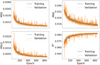 |
Fig. 3 Training history of the NN using the GRU architecture in the case of Model A on Dataset-short. Each plot compares the metric on the training set (solid blue line) with its counterpart on the validation set (solid orange line). The training curve represents the model’s performance on the data it learns from, while the validation curve indicates its performance on a separate dataset (the validation dataset) during the training phase. |
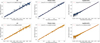 |
Fig. 4 Inferred model parameters compared with input model parameters for two cases: Dataset-short (top row) and Dataset-long (bottom row). Posteriors were calculated for 500 test spectra from the test dataset. The medians of the posteriors were derived from 1000 samples for each of the 500 test spectra, and the error on the median was determined from the 68% quantile of the distribution. A linear regression coefficient was calculated for each parameter across the 500 test samples. |
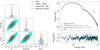 |
Fig. 5 Left: posterior distribution estimated for the reference spectrum with 2000 counts (red). The posterior distributions inferred from Bayesian fits with BXA and XSPEC are also shown in blue and green, respectively. Right: emission spectrum and residuals corresponding to the reference Model A with 2000 counts, together with the folded best-fit model from the GRU (solid green line) and XSPEC (dashed blue line) with a frequentist approach. |
3 Real data scenario
After demonstrating the effectiveness of our technique on simulated data, we verified its applicability to real data. This step is crucial in machine learning applications, as it determines the model’s ability to generalize and operate effectively on data not seen during training. We chose the same NICER observation of 4U 1820-30 analyzed by Barret & Dupourqué (2024) to facilitate model comparison. The analysis procedure for this source closely follows that of Barret & Dupourqué (2024) and is detailed in the following subsection. In the context of this study, we focus exclusively on analyzing the spectrum of the persistent X-ray emission.
3.1 Data reduction
Among low-mass X-ray binaries (LMXBs), 4U 1820-30 stands out due to its unique characteristics. It has the shortest known orbital period of any LMXB at just 11.4 minutes (Stella et al. 1987), classifying it as an ultra-compact X-ray binary (for a review, see Armas Padilla et al. 2023). Additionally, it belongs to a subclass known as X-ray bursters, characterized by periodic, rapid increases in luminosity, called Type I X-ray bursts, caused by thermonuclear burning of hydrogen and heavier elements at the neutron star surface.
4U 1820-30 has been observed multiple times by NICER. To compare our results with those obtained by Barret & Dupourqué (2024), we analyzed the same observation referenced by the authors, specifically the one from October 28, 2017 (ObsID 1050300108), with a total exposure time of 29 ks. We processed the NICER data using the nicer12 pipeline tool in NICERDAS v12, available with HEASoft v6.34, following the recommended calibration procedures and standard screening (the calibration database version used was xti20240206). We generated the light curve in the 0.3–10 keV range using nicerl3-lc to check for Type-I X-ray bursts, identifying one. To focus on analyzing the persistent spectrum, we excluded the burst by selecting a time interval outside of it. Specifically, we extracted the spectrum from a time window of 190 seconds, starting 200 seconds before and ending 10 seconds prior to the burst, using nicerl3-spect and excluding detectors 14 and 34 due to their elevated noise levels. We used the scorpeon background file with the bkgformat=file option for background subtraction. Following the NICER team recommendations, we applied a systematic error of 1.5% and grouped the data with optimal rebinning (grouptype=optmin) with the additional requirement of a minimum number of 25 counts per energy bin (Kaastra & Bleeker 2016).
3.2 Training and predictions
The NICER spectrum can be described by a combination of a power law component and a black-body emission, bbodyrad in XSPEC (Arnaud 1996), both corrected for interstellar medium absorption using the model tbabs. The bbodyrad normalization is directly related to the radius of the emission region Rbb through the formula: Kbb = (Rbb/D10kpc)2, where D10kpc is the source distance in units of 10 kpc. The chosen model, referred to as Model B, is therefore: tbabs × (powerlaw + bbodyrad).
The first step is, therefore, to train a NN with this specific model to ensure that it learns the relevant parameter relationships. We generated a dataset of 3 × 10⁵ simulated spectra to accomplish this, following the same procedure outlined in the previous section. The ranges of the model parameters explored in these simulations are reported in Table 4. For reference, we show in Fig. 7 the source emission spectrum with 100 randomly selected simulated spectra. As in our earlier tests, both the input spectra and the corresponding output parameters were preprocessed. Specifically, we standardized the simulated spectra and normalized the model parameters using the methods described in Sect. 2.1. This preprocessing step was essential to ensure stable training and improve the convergence of the NN models.
We again tested three different NN architectures: ANN, CNN+ANN, and GRU, using the hyperparameters listed in Table 5. Also in this case (see Table 6), the GRU architecture consistently outperforms the others, making it the best choice for this task. We proceeded with the GRU model.
In Fig. 8, we highlight how the XSPEC fitting procedure, when using χ2 minimization, can become trapped in local minima, leading to significantly incorrect parameter estimates, as previously noted by Parker et al. (2022). This is particularly clear from the outliers that deviate from the expected correlation line, shedding light on cases where the optimization fails to find the global minimum. This effect is further explored in Fig. 9, where we compare the parameter estimated with our NN and those derived from XSPEC. The presence of outliers in the XSPEC results confirms that local minima can lead to inaccurate parameter estimates. In contrast, our GRU-based NN significantly reduces this risk. While our method does not always achieve the same level of precision as XSPEC when XSPEC converges correctly, it consistently avoids false minima, ensuring stable and reliable parameter estimates across different cases.
In Fig. 10, we present the results of our model’s predictions on real data using the MonteXrist method. The first panel (left) shows the posterior distributions of the model parameters, as inferred by our GRU-based MonteXrist approach, alongside results from BXA and XSPEC MCMC. The MonteXrist results (in red) are well-aligned with the other methods, demonstrating comparable parameter distributions and effectively capturing the correlations between parameters. The figure also highlights the model’s ability to approximate the posterior distributions typically obtained via traditional Bayesian inference approaches. Beyond achieving comparable results, a key strength of our method is its efficiency: MonteXrist, after the training phase, reaches these results in approximately one-tenth of the time required by BXA, using the same computational resources. This clear advantage highlights the potential of MonteXrist for faster, yet accurate, parameter estimation in X-ray astronomy.
In the second panel (right) in Fig. 10, we display the best-fit emission spectrum obtained from XSPEC’s frequentist approach (dashed blue line) and compare it with the median prediction from MonteXrist method (solid green line), superimposed on the observed data (black points). The lower plot shows the residuals of both fits, with XSPEC residuals (blue points) and MonteXrist residuals (green points) relative to the observed data.
Although both methods fit the spectral shape well, there is a slight difference in the residuals, especially at lower energies. This discrepancy arises from a higher normalization value for the blackbody component (bbodyrad) obtained with the Mon- teXrist results compared to ones obtained with the XSPEC fit. A higher normalization in bbodyrad implies a stronger contribution from the thermal component, which could account for the slightly elevated residuals observed in the MonteXrist fit at lower energies. Overall, the χ2/d.o.f. values are 0.9 for XSPEC and 1.03 for MonteXrist, indicating that the MonteXrist approach provides results comparable to traditional methods. This illustrates that MonteXrist serves as a viable alternative for parameter estimation, providing robust uncertainty quantification through posterior distributions. The method has proven to be effective not only on simulated data but also on real observational data, highlighting its potential for practical applications in X-ray astronomy.
A possible way to enhance performance is by restricting the prior distributions of model parameters, as done in Barret & Dupourqué (2024). While this approach can improve results by focusing the training on the most relevant regions of parameter space, our aim is to develop a tool with the as broad as possible applicability. By preserving full flexibility in the prior distributions, MonteXrist can be applied to a wider range of cases without requiring case-specific adjustments, making it particularly suitable for large-scale and high-resolution spectral studies.
Parameter ranges for Model B.
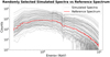 |
Fig. 7 Emission spectrum from 4U 1820-30 (red line) and 100 randomly selected simulated (Model B) spectra from the prior distribution (gray lines). |
Hyperparameters used in the NNs for Model B.
Evaluation of results for Model B.
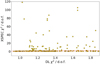 |
Fig. 8 Comparison of XSPEC spectral fitting (χ2 minimization) and predictions from the trained GRU NN for the Model B. The dashed red line represents the expected 1:1 correlation. Points that deviate significantly from this line indicate cases where XSPEC became trapped in a local minimum, highlighting the robustness of the NN approach in avoiding false minima. |
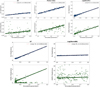 |
Fig. 9 Similar to Fig. 4. The top panels (blue points) employ the trained GRU NN, while the bottom panels (green points) use XSPEC with Bayesian inference disabled, for the Model B. |
4 Discussion and conclusions
We have developed and tested a NN-based approach for X-ray spectral fitting, applying MCD (referred to as Mon- teXrist) to infer spectral model parameters and their uncertainties. We trained and validated this method on simulated data, demonstrating its ability to recover parameter distributions that are comparable to those obtained via traditional Bayesian methods, such as MCMC and BXA. To benchmark our method, we performed tests using the same datasets as Barret & Dupourqué (2024), facilitating a direct comparison of the two approaches. A possible way to refine parameter estimation is by narrowing the prior parameter space, as done in Barret & Dupourqué (2024) using techniques such as ResNet-based classifiers or coarse-to- fine inference. While it can improve performance by focusing the inference on the most relevant regions of parameter space, our approach is designed to operate directly on the full prior distributions. This ensures that MonteXrist remains broadly applicable, capable of handling a wide variety of datasets without requiring tailored preprocessing steps, making it particularly suitable for large-scale and high-resolution spectral studies. This study serves as a proof of concept, illustrating the potential of NNs for X-ray spectral analysis and setting the groundwork for future exploration. However, further testing on a broader range of models and datasets is necessary to fully assess the robustness and general applicability of this approach.
It is important to recognize the known limitations of the MCD approach. Since it approximates Bayesian inference, which can be less accurate and less detailed than a full Bayesian inference, it may not capture all the nuances of the true posterior distributions. Moreover, the uncertainty estimates produced by the method are influenced by factors such as the dropout rate and the specific value the network is attempting to estimate, which can introduce additional variability in the results (Verdoja & Kyrki 2020). Nonetheless, our strategy offers significant advantages for high-throughput applications, such as those expected in upcoming astronomical missions, which will produce large datasets that might require rapid and automated analysis. The MonteXrist approach mitigates the risk of local minima trapping, a common challenge in traditional spectral fitting, while achieving comparable precision to established frequentist methods without requiring the application of methods for restricting the range of the prior distribution of parameters. Moreover, one of the key strengths of our method is its efficiency in inference time post-training. In our tests on real data, BXA required approximately 10 minutes to produce a posterior chain of sufficient length, while MonteXrist completed the same task in about 1 minute, a considerable improvement in speed. Additionally, the dataset generation process takes approximately 10 minutes when executed on a single processor, and training the GRU model requires about one day using an NVIDIA GeForce RTX 4080. It is important to note that the code used for managing input and output operations has not been optimized for performance, leaving room for further improvements. This efficiency makes our approach particularly appealing for real-time or near-real-time applications, where rapid parameter estimation and uncertainty quantification are essential.
An interesting future extension of this work would involve the use of principal component analysis (PCA; Pearson 1901; Del Santo et al. 2008; Jolliffe & Cadima 2016) to reduce the dimensionality of the spectral data. PCA is a statistical technique that transforms the original data into a new set of uncorrelated variables, known as principal components, that capture the directions of maximum variance in the data. By retaining only the most significant components, PCA efficiently reduces the number of features while preserving most of the original data’s information. In the context of spectral fitting, PCA could help decrease the input dimensionality, accelerating the training process, especially for complex architectures such as GRUs, without compromising the accuracy. This approach would be particularly beneficial for high-resolution spectra with a large number of features, where dimensionality reduction could alleviate the computational burden and improve efficiency. Previous studies, including Barret & Dupourqué (2024) and Parker et al. (2022), have shown that PCA maintains comparable precision while significantly speeding up the training, making it a valuable tool for enhancing computational performance in scenarios with high-dimensional data.
Additionally, optimizing the network architecture and hyperparameters could further enhance model performance. While we used a standard set of hyperparameters in this study, a more systematic hyperparameter tuning, especially for the dropout rate, could yield improvements in both accuracy and uncertainty quantification. Determining the optimal dropout value is crucial for balancing regularization and capturing realistic uncertainty distributions.
A compelling future direction for this research may encompass the use of Bayesian neural networks (BNNs; MacKay 1992; Magris & Iosifidis 2023) as an alternative to MCD for quantifying parameter uncertainties in spectral fitting tasks. Unlike the MCD approach, which approximates Bayesian inference by randomly deactivating neurons during inference, BNNs provide a true Bayesian formulation. This feature could prove particularly valuable in scenarios where accurate uncertainty estimation is critical, such as in low-count spectra or observations with high noise levels. However, the use of BNNs also presents notable challenges. The primary drawback of BNNs is their computational expense, as methods like variational inference and Markov chain Monte Carlo sampling, which are commonly used to estimate the posterior distribution, can significantly increase training times. This could restrict the application of BNNs in large-scale spectral analysis or real-time data processing scenarios. Furthermore, training BNNs requires advanced Bayesian optimization techniques and often involves careful hyperparameter tuning to achieve optimal results, adding to the complexity and development time.
Despite these challenges, BNNs remain a promising alternative for uncertainty quantification in X-ray spectral fitting, especially as astronomical missions continue to produce increasingly large datasets that demand efficient, automated analysis. Future work could explore ways to integrate BNNs with high- performance computing resources and advanced optimization techniques to balance accuracy with computational feasibility. As such, BNNs offer a compelling direction for future research, with the potential to provide robust and reliable uncertainty estimates that complement the strengths of MCD in scalable, real-time applications.
In summary, our MonteXrist method is a promising alternative to traditional spectral fitting approaches, particularly for large datasets anticipated from future missions. While some challenges remain, this framework has the potential to become a valuable tool in X-ray spectral analysis, enabling fast, reliable, and interpretable inference that scales effectively with the data volume.
Acknowledgements
We acknowledge the useful comments and suggestions of the referee, which improved the manuscript. We thank Alessandra Robba for the valuable discussions. A.T., A.P., A.Z. acknowledge supercomputing resources and support from ICSC – Centro Nazionale di Ricerca in High Performance Computing, Big Data and Quantum Computing – and hosting entity, funded by European Union – NextGenerationEU. A.T., A.A. acknowledge support from INAF Mini Grants DREAM-XS (Deep Recurrent Analysis and Modeling for X-ray Spectroscopy). C.P., F.P. acknowledge support from PRIN MUR SEAWIND funded by European Union – NextGenerationEU, INAF Grants BLOSSOM and OBIWAN (Observing high B-fIeld Whispers from Accreting Neutron stars, 1.05.23.05.12). R.L.P. acknowledges support from INAF’s research grant Uncovering the optical beat of the fastest magnetised neutron stars (FANS) and from the Italian Ministry of University and Research (MUR), PRIN 2020 (prot. 2020BRP57Z) Gravitational and Electromagnetic-wave Sources in the Universe with current and next-generation detectors (GEMS). E.A. acknowledges funding from the Italian Space Agency, contract ASI/INAF no. I/004/11/4.
References
- Abadi, M., Agarwal, A., Barham, P., et al. 2015, TensorFlow: Large-Scale Machine Learning on Heterogeneous Systems, software available from tensorflow.org [Google Scholar]
- Armas Padilla, M., Corral-Santana, J. M., Borghese, A., et al. 2023, A&A, 677, A186 [NASA ADS] [CrossRef] [EDP Sciences] [Google Scholar]
- Arnaud, K. A. 1996, in Astronomical Data Analysis Software and Systems V, eds. G. H. Jacoby, & J. Barnes, Astronomical Society of the Pacific Conference Series, 101, 17 [NASA ADS] [Google Scholar]
- Barret, D., & Dupourqué, S. 2024, A&A, 686, A133 [NASA ADS] [CrossRef] [EDP Sciences] [Google Scholar]
- Barret, D., Albouys, V., Herder, J.-W. D., et al. 2023, Exp. Astron., 55, 373 [NASA ADS] [CrossRef] [Google Scholar]
- Bégué, D., Sahakyan, N., Dereli-Bégué, H., et al. 2024, ApJ, 963, 71 [CrossRef] [Google Scholar]
- Bishop, C. M. 1995, Neural Networks for Pattern Recognition (Oxford University Press) [Google Scholar]
- Buchner, J., Georgakakis, A., Nandra, K., et al. 2014, A&A, 564, A125 [NASA ADS] [CrossRef] [EDP Sciences] [Google Scholar]
- Cho, K., van Merrienboer, B., Gulcehre, C., et al. 2014, arXiv e-prints [arXiv:1406.1078] [Google Scholar]
- Chollet, F. et al. 2015, Keras, https://keras.io [Google Scholar]
- Del Santo, M., Malzac, J., Jourdain, E., Belloni, T., & Ubertini, P. 2008, MNRAS, 390, 227 [NASA ADS] [CrossRef] [Google Scholar]
- Gal, Y., & Ghahramani, Z. 2015, arXiv e-prints [arXiv:1506.02142] [Google Scholar]
- Gendreau, K. C., Arzoumanian, Z., & Okajima, T. 2012, SPIE Conf. Ser., 8443, 844313 [Google Scholar]
- Goodfellow, I., Bengio, Y., & Courville, A. 2016, Deep Learning (MIT Press), http://www.deeplearningbook.org [Google Scholar]
- Gordon, C., & Arnaud, K. 2021, PyXspec: Python interface to XSPEC spectral-fitting program, Astrophysics Source Code Library [record ascl:2101.014] [Google Scholar]
- He, K., Zhang, X., Ren, S., & Sun, J. 2016, in 2016 IEEE Conference on Computer Vision and Pattern Recognition (CVPR), 1 [Google Scholar]
- Ichinohe, Y., Yamada, S., Miyazaki, N., & Saito, S. 2018, MNRAS, 475, 4739 [NASA ADS] [CrossRef] [Google Scholar]
- Jolliffe, I., & Cadima, J. 2016, Philos. Trans. Roy. Soc. A: Math. Phys. Eng. Sci., 374, 20150202 [NASA ADS] [CrossRef] [Google Scholar]
- Kaastra, J. S., & Bleeker, J. A. M. 2016, A&A, 587, A151 [NASA ADS] [CrossRef] [EDP Sciences] [Google Scholar]
- Kaastra, J. S., Mewe, R., & Nieuwenhuijzen, H. 1996, in UV and X-ray Spectroscopy of Astrophysical and Laboratory Plasmas, eds. K. Yamashita & T. Watanabe, 411 [Google Scholar]
- Kingma, D. P., & Ba, J. 2014, CoRR, abs/1412.6980 [Google Scholar]
- Lecun, Y., Bottou, L., Bengio, Y., & Haffner, P. 1998, Proc. IEEE, 86, 2278 [Google Scholar]
- MacKay, D. J. C. 1992, Neural Computat., 4, 448 [Google Scholar]
- Magris, M., & Iosifidis, A. 2023, Bayesian Learning for Neural Networks: An Algorithmic Survey [Google Scholar]
- Parker, M. L., Lieu, M., & Matzeu, G. A. 2022, MNRAS, 514, 4061 [NASA ADS] [CrossRef] [Google Scholar]
- Pearson, K. 1901, London Edinb. Dublin Philos. Mag. J. Sci., 2, 559 [CrossRef] [Google Scholar]
- Pedregosa, F., Varoquaux, G., Gramfort, A., et al. 2011, J. Mach. Learn. Res., 12, 2825 [Google Scholar]
- Predehl, P., Andritschke, R., Arefiev, V., et al. 2021, A&A, 647, A1 [EDP Sciences] [Google Scholar]
- Srivastava, N., Hinton, G., Krizhevsky, A., Sutskever, I., & Salakhutdinov, R. 2014, J. Mach. Learn. Res., 15, 1929 [Google Scholar]
- Stella, L., White, N. E., & Priedhorsky, W. 1987, ApJ, 315, L49 [Google Scholar]
- Tashiro, M., Maejima, H., Toda, K., et al. 2018, in Space Telescopes and Instrumentation 2018: Ultraviolet to Gamma Ray, 10699, eds. J.-W. A. den Herder, S. Nikzad, & K. Nakazawa, International Society for Optics and Photonics (SPIE), 1069922 [Google Scholar]
- Tzavellas, A., Vasilopoulos, G., Petropoulou, M., Mastichiadis, A., & Stathopoulos, S. I. 2024, A&A, 683, A185 [NASA ADS] [CrossRef] [EDP Sciences] [Google Scholar]
- Verdoja, F., & Kyrki, V. 2020, arXiv e-prints [arXiv:2008.02627] [Google Scholar]
- Verner, D. A., Ferland, G. J., Korista, K. T., & Yakovlev, D. G. 1996, ApJ, 465, 487 [Google Scholar]
- Wilms, J., Allen, A., & McCray, R. 2000, ApJ, 542, 914 [Google Scholar]
All Tables
All Figures
|
Fig. 1 Distribution of total counts for the spectra in the two datasets. The blue histogram represents the dataset based on the reference spectrum with approximately 2 × 10³ total counts (Dataset-short). In comparison, the orange histogram corresponds to the dataset based on the reference spectrum with approximately 2 × 10⁴ total counts (Dataset- long). Both distributions illustrate the variability in total counts due to the range of parameters used in the simulations. Vertical dashed lines show the position of the two reference spectra. |
| In the text | |
|
Fig. 2 Model architecture used for training in the case of ANN and GRU models. The yellow blocks represent either GRU layers or ANN layers, depending on the chosen architecture. The red blocks correspond to dropout layers modified to remain active during inference, enabling posterior distribution sampling for uncertainty quantification. The final blue block is a dense layer that maps the learned features to the output parameters, such as spectral model components. |
| In the text | |
|
Fig. 3 Training history of the NN using the GRU architecture in the case of Model A on Dataset-short. Each plot compares the metric on the training set (solid blue line) with its counterpart on the validation set (solid orange line). The training curve represents the model’s performance on the data it learns from, while the validation curve indicates its performance on a separate dataset (the validation dataset) during the training phase. |
| In the text | |
|
Fig. 4 Inferred model parameters compared with input model parameters for two cases: Dataset-short (top row) and Dataset-long (bottom row). Posteriors were calculated for 500 test spectra from the test dataset. The medians of the posteriors were derived from 1000 samples for each of the 500 test spectra, and the error on the median was determined from the 68% quantile of the distribution. A linear regression coefficient was calculated for each parameter across the 500 test samples. |
| In the text | |
|
Fig. 5 Left: posterior distribution estimated for the reference spectrum with 2000 counts (red). The posterior distributions inferred from Bayesian fits with BXA and XSPEC are also shown in blue and green, respectively. Right: emission spectrum and residuals corresponding to the reference Model A with 2000 counts, together with the folded best-fit model from the GRU (solid green line) and XSPEC (dashed blue line) with a frequentist approach. |
| In the text | |
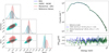 |
Fig. 6 Same as Fig. 5 but for the reference spectrum with 2 × 10⁴ counts. |
| In the text | |
|
Fig. 7 Emission spectrum from 4U 1820-30 (red line) and 100 randomly selected simulated (Model B) spectra from the prior distribution (gray lines). |
| In the text | |
|
Fig. 8 Comparison of XSPEC spectral fitting (χ2 minimization) and predictions from the trained GRU NN for the Model B. The dashed red line represents the expected 1:1 correlation. Points that deviate significantly from this line indicate cases where XSPEC became trapped in a local minimum, highlighting the robustness of the NN approach in avoiding false minima. |
| In the text | |
|
Fig. 9 Similar to Fig. 4. The top panels (blue points) employ the trained GRU NN, while the bottom panels (green points) use XSPEC with Bayesian inference disabled, for the Model B. |
| In the text | |
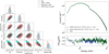 |
Fig. 10 Same as Figs. 5 and 6 but for the spectrum of source 4U 1820-30. |
| In the text | |
Current usage metrics show cumulative count of Article Views (full-text article views including HTML views, PDF and ePub downloads, according to the available data) and Abstracts Views on Vision4Press platform.
Data correspond to usage on the plateform after 2015. The current usage metrics is available 48-96 hours after online publication and is updated daily on week days.
Initial download of the metrics may take a while.