| Issue |
A&A
Volume 699, July 2025
|
|
|---|---|---|
| Article Number | A174 | |
| Number of page(s) | 11 | |
| Section | Cosmology (including clusters of galaxies) | |
| DOI | https://doi.org/10.1051/0004-6361/202555237 | |
| Published online | 07 July 2025 | |
Cosmological constraints with void lensing
I. Simulation-based inference framework
1
Shanghai Astronomical Observatory (SHAO), Nandan Road 80, Shanghai 200030, China
2
University of Chinese Academy of Sciences, Beijing 100049, China
3
Department of Astronomy, Tsinghua University, Beijing 100084, China
⋆ Corresponding authors: This email address is being protected from spambots. You need JavaScript enabled to view it.
; This email address is being protected from spambots. You need JavaScript enabled to view it.
; This email address is being protected from spambots. You need JavaScript enabled to view it.
Received:
21
April
2025
Accepted:
23
May
2025
Abstract
We present a simulation-based inference (SBI) framework for cosmological parameter estimation via a void-lensing analysis. Despite the absence of an analytical model of void lensing, SBI can effectively learn posterior distributions through forward modeling of mock data. We developed a forward modeling pipeline that accounts for both the cosmology and the galaxy-halo connection. By training a neural density estimator (NDE) on simulated data, we were able to infer the posteriors of two cosmological parameters, Ωm and S8. Validation tests were conducted on posteriors derived from different cosmological parameters and a fiducial sample. The results demonstrate that SBI provides unbiased estimates of mean values and accurate uncertainties. These findings also highlight the potential for applying void-lensing analyses to observational data – even without an analytical void-lensing model.
Key words: cosmological parameters / dark matter / large-scale structure of Universe
© The Authors 2025
 Open Access article, published by EDP Sciences, under the terms of the Creative Commons Attribution License (https://creativecommons.org/licenses/by/4.0), which permits unrestricted use, distribution, and reproduction in any medium, provided the original work is properly cited.
This article is published in open access under the Subscribe to Open model. This email address is being protected from spambots. You need JavaScript enabled to view it. to support open access publication.
1. Introduction
The large-scale structure of dark matter contains useful information about our Universe. Since dark matter does not interact with photons, its large-scale distribution should be traceable by visible proxies such as galaxies. By measuring the statistics of galaxies, such as the clustering of galaxies and the distortions of galaxy shapes caused by gravitational lensing, we can analyze the underlying distributions of dark matter and set constraints on the ΛCDM model, which provides the best description of our Universe today. Recent observational data from spectroscopic surveys such as Sloan Digital Sky Survey (SDSS, Eisenstein et al. 2011; Dawson et al. 2012) and Dark Energy Survey Instrument (DESI, DESI Collaboration 2016a, b), as well as photometric surveys such as Kilo-Degree Survey (KiDS, Heymans et al. 2021), Dark Energy Survey (DES, Bechtol et al. 2025), and Hyper Suprime-Cam (HSC, Aihara et al. 2017) have raised the constraints on cosmological parameters to an unprecedented level of precision. Recently, two new analyses from the latest released data have provided fresh insights into our understanding of the Universe. One comes from DESI DR2 BAO measurements (with CMB and supernovae measurements) (DESI Collaboration 2025), which shows a ∼3σ deviation from ΛCDM model, preferring an evolving dark energy rather than a cosmological constant. The other comes from the cosmic shear analysis with the latest KiDS-Legacy data (Wright et al. 2025), showing that the cosmological parameter,  , is in agreement with results from Planck CMB. The upcoming next-generation photometric surveys such as Euclid (Laureijs et al. 2011), Legacy Survey of Space and Time (LSST, LSST Science Collaboration 2009), and China Space Station Telescope (CSST, Gong et al. 2019; Zhan 2021), as well as spectroscopic surveys such as MUST (Zhao et al. 2024), are expected to further improve the constraints and enhance our knowledge of the Universe with the help of the deeper and wider survey areas, coupled with higher data quality.
Basic cosmological data analyses rely on analyzing “summary statistics” compressed from raw observational data, such as the power spectrum P(k). By applying a data compression, we can greatly reduce the dimension of the data vector, making it easier to deduce the theoretical models for the compressed summary statistics. At present, two point (2pt) statistics are the most used summary statistics in cosmological analysis, which contain complete information of a Gaussian random field. Since large-scale cosmological fields, such as the dark matter density field, are widely approximated as Gaussian fields, most of the cosmological information has been included in the two-point statistics. In recent decades, this analytical framework has been confirmed to be greatly successful by large amounts of literature (Gil-Marín et al. 2015; Heymans et al. 2021; Singh et al. 2019; Yao et al. 2023; Asgari et al. 2021; Wenzl et al. 2024).
In recent years, with the great development of observational data, it has become increasingly appealing to extract non-Gaussian information from cosmological fields. A variety of analysis techniques beyond two-point statistics have been developed in recent decades and have been proven to provide better constraints on the cosmological model (Halder et al. 2023; Lai et al. 2024; Ivanov et al. 2023; Burger et al. 2023; Harnois-Déraps et al. 2021; Heydenreich et al. 2021; Cheng et al. 2024). Void statistics, such as void abundance (the number density as a function of void size, Rv), void clustering, and void lensing are one class of statistics that is beyond traditional two-point statistics. Voids are large-scale underdense regions in the cosmic web filling most of the space of the Universe. Due to its underdense nature, dark matter structures in voids are less affected by nonlinear growth. Meanwhile, two-point statistics of voids can contain information encoded in galaxy high order statistics, since when we correlate two voids, we are actually correlating 2N galaxies if we use N galaxies to define a void. These recent advantages have encouraged researchers to use voids to study the distributions and evolutions of dark matter (Pisani et al. 2019; Kreisch et al. 2022; Boschetti et al. 2024; Chantavat et al. 2016, 2017), the mass of neutrino (Massara et al. 2015; Thiele et al. 2024; Bayer et al. 2021; Kreisch et al. 2022), and the nature of gravity (Cai et al. 2015; Wilson & Bean 2021; Su et al. 2023).
However, to shed light on the large scale structure of dark matter by use of voids, we are faced with a number of challenges. First, it is challenging to build an accurate model for some void statistics. In particular, there are very few models that can accurately describe the void-lensing statistics, the cross-correlation between void position and shapes of background galaxies1. The diversity of definitions of void also brings many difficulties in void statistics modeling. Another problem of void statistics is that void is identified based on the galaxy catalog; therefore, in addition to cosmology, the galaxy formation process would also be expected to influence the void statistics. The cosmological structure formation and the galaxy-halo connections should be simultaneously considered in the inference process to obtain an unbiased estimation of cosmological parameters. Both of those challenges call for new techniques.
Recently, machine learning (ML) techniques have become popular in astrophysics and cosmology. With the help of ML, simulation-based inference (SBI)2 has been developed to deal with cosmological inferences. Regardless of whether we have an explicit likelihood or not, in a Bayesian data analysis, we are just aiming to obtain a posterior of the model parameters. The principle of SBI instead calls for the construction of an implicit posterior (or the likelihood or the ratio of the likelihood and the prior), which can be learned directly from the simulation data by training a neural network. Therefore, SBI can be applied to any statistics that can be simulated, regardless of whether it has a theoretical model available. Plenty of successful applications of SBI in different fields of cosmology have been presented. For example, in the context of weak-lensing studies, von Wietersheim-Kramsta et al. (2025) constructed a systematical analysis pipeline for the analysis of cosmic shear for KiDS-1000 survey. Later Jeffrey et al. (2024) presented an SBI analysis to infer wCDM model parameters using DES-Y3 data. Novaes et al. (2024) used SBI to analyze HSC-Y1 weak-lensing data to explore the performance of high-order statistics. Another example is the SIMulation-Based Inference of Galaxies (SIMBIG) project (Lemos et al. 2023a; Hahn et al. 2023a, b,c, 2024; Massara et al. 2024; Hou et al. 2024; Régaldo-Saint Blancard et al. 2024), which presents series works to construct the SBI analysis pipeline to set cosmological constraints on cosmology using galaxy clustering. In particular, these authors simultaneously considered the cosmological and galaxy-halo connection (halo occupation distribution, HOD) models, which provide a significant reference in studying galaxy-based cosmological probes. SBI has also been applied in other fields of cosmology, including research on strong lensing, the epoch of reionization, and neutrino mass (Poh et al. 2022; Zhao et al. 2022; Thiele et al. 2024).
In this work, we apply SBI on the void-lensing statistics and explore the constraining power on cosmological parameters. Motivated by the series work of SIMBIG, we built a similar workflow of the inference, but changing most of the details. First, due to the large scale sensitivity of void-lensing signals, we used a fast particle-mesh simulation, rather than high-fidelity N-body simulation to construct the training set and validation set. This allows us to generate a larger amount of training sets with a relatively small cost. Besides, the galaxy-halo connection is taken into account through the halo abundance matching (HAM) technique (Rodríguez-Torres et al. 2016; Yu et al. 2022, 2023). Compared with HOD, the advantage of HAM is that there are fewer model parameters, thereby simplifying the training process. Finally, our statistics are different from the galaxy clustering. The result will be complementary to the constraining results presented here.
The rest of the paper is organized as follows. In Sect. 2, we introduce the SBI, including the motivation and workflow. In Sect. 3, we describe our forward modeling pipeline in detail, where we also introduce void-lensing statistics, the main statistics considered in this work. After presenting the training and validation procedures in Sect. 4, we give our results in Sect. 5. Our conclusions and future plans are shown in Sect. 6.
2. Method: SBI
2.1. Motivation
In Bayesian inference, we are concerned with the posterior probability distribution p(θ|d) of model parameters, θ, given some observed data, d. From the Bayes Theorem, the posterior can be written as:
 (1)
(1)
where p(d|θ) is called likelihood function, p(θ) is the prior distribution of parameter θ, and p(d) is the Bayesian evidence which is useful in model selection tasks. Through Eq. (1), the estimation of posterior p(θ|d) can be transformed to the estimation of likelihood p(d|θ). In practice, the likelihood is usually chosen as a Gaussian distribution, with the mean of the data vector and the covariance of the data covariance, C. Assuming the model is a mapping f:θ→d, the likelihood can be expressed as:
![Mathematical equation: $$ p(\boldsymbol {d}|\boldsymbol {\theta }) \propto \exp {\left [\frac {1}{2}(\boldsymbol {d}-f(\boldsymbol {\theta }))^T \boldsymbol {C}^{-1} (\boldsymbol {d}-f(\boldsymbol {\theta }))\right ]}. $$](/articles/aa/full_html/2025/07/aa55237-25/aa55237-25-eq3.gif) (2)
(2)
The best-fit values of parameters can be obtained by the mean/median of the posterior, which can be estimated by Monte Carlo sampling such as a Markov chain Monte Carlo (MCMC).
The procedure above may fail when the calculation of the model f(θ) in Eq. (2) is not efficient or even inaccessible. Moreover, Eq. (2) can only describe a Gaussian likelihood function and might not work when likelihood is not Gaussian. In other words, our aim is to perform parameter inference in the context of an implicit likelihood. This motivates the SBI technique. Instead of an explicit formula of the likelihood, SBI only requires a set of samples whose distribution obeys the required likelihood function. In cosmology, these samples can usually be obtained by running cosmological simulations. Mathematically, this process actually samples parameter-data pairs {θ,d} from joint probability distribution, p(θ,d)∝p(d|θ)p(θ)∝p(θ|d). SBI can then learn the posterior, p(θ|d), or likelihood p(d|θ) from these samples with neural networks. In practice, SBI constructs the so-called density estimators3, qϕ(θ|d), and they will be optimized to approximate true underlying posterior or likelihood (which we refer to as target distribution) based on simulations. The ϕ appearing in the estimator represents free parameters to be optimized4. Then, it is possible to draw samples from this estimator, as can be done in traditional Bayesian inference, and analyze the mean and covariance of the model parameters as well.
2.2. Workflow
The basic workflow of SBI can be shown in Fig. 1: the first step is forward modeling, which transforms parameters to data vectors; then by use of parameter θ and the data, d, we can construct the neural density estimator qϕ(θ|d). After training the neural estimator, we can obtain an estimated likelihood and posterior. Accurate modeling is essential to obtain an accurate posterior estimator, and appropriate network structures and training strategies are helpful for optimizing the estimator.
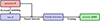 |
Fig. 1. Workflow of a typical SBI with neural posterior estimation (NPE), i.e., directly estimating the posterior. The forward modeling process transforms parameters to be inferred to data vector, and therefore includes the process of measuring summary statistics from simulation results in our case. The density estimator takes parameter-data pair {θ,d} as input, and after the training procedure returns an estimation of posterior. Note: for the neural likelihood estimation (NLE) and neural ratio estimation (NRE), the target to be trained (shown in green block) is the likelihood and the ratio of likelihood and prior, respectively. Combined with the prior, this allows us to easily build the posterior using Bayes law. |
The key point of SBI is the construction of density estimators as they will be proxies of the underlying true posteriors. Based on the type of target distributions, density estimators can generally be divided into the neural posterior estimator (NPE, which directly estimates the posterior p(θ|d)), the neural likelihood estimator (NLE, estimating the likelihood p(d|θ)), and the neural ratio estimator (NRE, estimating the ratio of posterior and prior p(θ|d)/p(θ)). In this work, we use the NPE to achieve our inference. Since the posterior is accessible, it is not necessary to run MCMC sampling to obtain the final constrain contour of parameters, which is computationally efficient. In the following part of the article, unless otherwise specified when we refer to “SBI”, we mean the NPE strategy of SBI.
There are several existing networks to construct density estimators, two of which are the mixture density network (MDN) and masked autoregressive flows (MAFs). The MDN can be intuitively understood as a fitting procedure that fits the target posterior by many Gaussian components with different means and covariance matrices. We can train a neural network to learn a set of appropriate means and covariance matrices. The principle of MAFs is based on the chain rule of probability demonstrating that any joint probability distribution, p(x), can be decomposed into productions of a series of 1D conditional probability distributions as  . If the beginning of the chain is a standard normal distribution and each of the conditional probabilities is invertible, then this can be regarded as a normalization flow from p(x) to a standard normal distribution, which makes p(x) easy to sample. As a density estimator, MAFs actually learn these conditional probabilities by some parameterized functions qϕ(x). In practice, we can either use one kind of network architecture or use an ensemble of different architectures to construct the density estimators, so as to achieve better performance.
After determining the density estimator, the next step is to prepare training and validation sets. This is another key process in SBI since all of the information is learned from the training sets. In the following, we introduce our forward modeling pipeline, where we start with the dark matter field and, finally, we describe our summary statistics.
3. Forward modeling
In this section, we describe our forward-modeling pipeline in detail. Figure 2 shows the flowchart of our pipeline. At the start, we input the cosmological parameters, generated the initial dark matter distributions, and ran simulations to obtain the dark matter field at the present time. We then applied the halo finder algorithm on the dark matter field to identify dark matter halos. Galaxies are then populated to halos through halo abundance matching (HAM) method. The voids were identified in the galaxy catalog and, finally, we could measure the void-lensing signals.
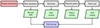 |
Fig. 2. Schematic diagram of forward modeling. The gray blocks represent modeling processes, the green blocks represent outputs in each step of modeling. The red block represents input parameters in the model. The gray blocks represent steps in forward modeling and the green blocks show the corresponding output in each step. The final output i.e., the void-lensing signal is shown in blue. |
3.1. FastPM simulation
FASTPM5 (Feng et al. 2016) is a particle-mesh (PM) simulation that trade-off the accuracy for speed as compared to N-body simulations. It maps the particles used in mesh grids to estimate the gravitational force; therefore, the loss accuracy on scales smaller than grid size. Besides, it modifies the traditional kick and drift factor to ensure the correctness of linear displacement evolution on large scales, regardless of the number of time steps.
In this work, we ran FASTPM with 10243 dark matter particles in a 1 h−1 Gpc box. The force resolution, B, which is the ratio between mesh size and number of particles, was chosen as B = 2. Then 40 linear steps were used to evolve the density field from a = 0.01 to a = 1. We note that it is typical to run FastPM at a = 0.1 to avoid transient noise; however, we tested the power spectra of different initial redshifts and found that the differences are negligible compared with the differences between FastPM and high-fidelity N-body simulations. Therefore, it will not greatly influence our results.
Because of the limitation of computing resources, in this work, we only considered two cosmological parameters that are expected to be sensitive to lensing statistics: the matter density parameter, ΩM, and the standard deviation of matter density fluctuation in 8 h−1 Mpc, σ8. Due to the well-known degeneracy between these two parameters (e.g., the “banana-shaped” contour on ΩM−σ8 plane for cosmic shear statistics), we chose  to replace the original σ8 parameter. Thus, the cosmological parameter space is constructed by ΩM and S8. We sampled independent 1000 parameter pairs from the priors,
  and
and  , where
  represents uniform distribution. The upper left of Fig. 3 provides a visualization of distributions of cosmological parameter samples. These 1000 parameters are then as the input of FASTPM to generate dark matter fields. In order to consider the variety in p(θ,d) along dimensions of data, d, we used different random seeds for each cosmological simulation.
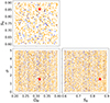 |
Fig. 3. Parameter space of parameters considered in this work, including cosmological parameters ΩM, S8, and HAM parameter, σ. These samples are randomly divided into two parts with 9:1, corresponding to the training set (orange dots) and validation set (blue dots), respectively. To test the performance of our method on a special cosmology, we chose a fiducial cosmology marked as red star. Note: this sample is neither in the training set, nor the validation set. |
3.2. Galaxy and void catalogs
We first constructed the dark matter halo catalog. We chose the ROCKSTAR (Behroozi et al. 2012) software to find halos. This algorithm considers 6D phase space information to identify halos, which has been tested in some previous works (e.g., Thiele et al. 2024) and performs well in FASTPM.
Voids can be identified in either halo catalogs or galaxy catalogs. Since halos cannot be observed directly in real observation, it is better to choose galaxies as tracers of voids. This means galaxy-halo connection should be considered in the modeling. Halo abundance matching (HAM) is a simple and intuitive empirical method to describe the galaxy-halo connection. It is based on the assumption that there is a monotonic relation (not necessarily linear) between the galaxy luminosity (or stellar mass) and the halo mass (or the circular velocity). In addition, to model the stochasticity in the galaxy–halo mass relation (Willick et al. 1997; Steinmetz & Navarro 1999), we considered a Gaussian scatter with a dispersion, σ (which, in the following, we call the “HAM parameter”) to the halo mass (Tasitsiomi et al. 2004). In practice, we first multiplied Sg to the halo mass, Mh, to obtain Mscat=Mh×Sg for each halo in the simulation, where  when
when  and
and  otherwise. We sorted these halos in descending order of Mscat, then populated a galaxy in the center of each halo in the catalog from the most massive ones to the least ones – until we get the expected number of HAM galaxies, Ngal=nrefVbox.
In principle, for each halo catalog one can fit some statistics (e.g., projected two-point correlation function, wp) to the real data in order to obtain an optimized σ corresponding to a realistic galaxy mock. However, simultaneously optimizing cosmological and HAM parameters is available for SBI, which is a more self-consistent method. Meanwhile, purely using SBI to analyze cosmology and galaxy-halo connection can naturally consider the correlations between cosmological and HAM parameters. Therefore, we set the HAM parameter, σ, to be a free parameter and try to train SBI to extract the influence from galaxy formation processes on void-lensing signals. Following Hahn et al. (2023b), we randomly sampled HAM parameters ten times from prior  for each cosmology, and finally we have 10 000 mock galaxy catalogs in total. We note that the matter-to-halo bias is considered by the shuffling process; therefore, marginalizing the HAM parameters is actually marginalizing both galaxy and halo biases. The reference number density of galaxies is chosen as nref = 3.5×10⁻⁴ (h/Mpc)3 to match the BOSS LOWZ LRG samples (Dawson et al. 2012).
At this point, we are ready to identify voids on the galaxy catalog. We used DIVE6 (Zhao et al. 2016) to construct our void catalog. This method applies Delaunay triangulation on the galaxy catalog and defines voids as the empty circumspheres constrained by tetrahedra of galaxies. The void center and radius are regarded as those of sphere. These voids were prepared for measurements of void-lensing signals in the next step.
3.3. Void-lensing measurement
The gravitational field of the foreground matter will bend the light rays emitted from the distant galaxies, which will change their luminosity and shape. The distortion of the galaxy shape can be quantified by tangential shear, γt. It is related to the so-called lensing convergence, κ:
 (3)
(3)
where κ is a weighted integral over comoving distance of matter density δm, which can be written as:
 (4)
(4)
and  is the mean convergence inner the sphere with radius, R. If we define the critical surface density, Σcrit,
 (5)
(5)
and we further assume that the foreground matter density is associated with an isolated object (which in this work is an isolated void), Eq. (4) can be expressed as:
 (6)
(6)
From Eqs. (3) and (6), we can see that by analyzing the distortion of the background galaxies, it is possible to catch up information of foreground matter density distribution, δm. Similar to the case of galaxy-galaxy lensing (where the foreground objects are galaxies), void lensing describes the light distortion effects when the foregrounds are voids. Due to the underdensity characteristic of voids, void lensing will provide a “minus” signal compared with galaxy-galaxy lensing.
In observation one often choose the excess surface mass density ΔΣ as the observable. This is related to previous quantities by:
 (7)
(7)
In the following, the phrasing “void-lensing signal” is another way to refer to the excess surface mass density of voids. From Eqs. (6) and (7), it can be found that the void-lensing signal is just an integral transform of void profiles. Therefore, in simulations, it can be obtained in an inverse method; namely, measuring the void profiles and transform to lensing signals. This can reduce a great amount of calculations compared with running a full ray-tracing simulation. In this work, we chose this approximate technique and left a more realistic modeling process to a future work.
Measuring void profiles in simulation is equivalent to measuring the void-dark matter cross correlation. We used PYFCFC7, a Python-wrapper of FCFC8 (Zhao 2023) to measure the correlation function. We calculated ΔΣ using Eqs. (6) and (7) as void-lensing signal. We first cut the voids into the void radius interval 15<Rv<25 Mpc/h and divide those voids into ten linearly size bins, each with a width of ΔRv = 1 Mpc/h. Next, for each void size bin we measure correlation functions in 15 logarithm separation bins with a range of r∈[0.1,3]Rv, where Rv is the void radius. Then, these correlation functions are stacked to construct a higher signal-to-noise ratio (S/N) signal. This leads to a data vector with a dimension of 15.
4. Training and validation
After the forward-modeling process, we ended up with 10 000 samples for SBI (1000 cosmologies × 10 HAMs per cosmology). These samples should first be separated into training and validation sets. Overall, 90% of the total samples were regarded as training samples, while the remaining were prepared for validation. We note that only 1000 samples are considered to be independent in terms of cosmological parameters. Therefore, the ratio of the number of independent cosmology samples between the training set and validation set was also expected to be 9:1. Therefore, we required that different HAM samples with the same cosmological parameters would not be divided into training and validation sets, but to be put into either training or validation set as a whole. In Fig. 3, we illustrate the distributions of training and validation sets with orange and blue dots, respectively.
In this work, we used the public code LTU-ILI9 (Ho et al. 2024) to train our density estimator, qϕ(θ|d). The masked autoregressive flows (MAFs) and mixture density network (MDN) were both used to construct the density estimator. For MAFs, we use five MADE blocks, each of which has 50 hidden features. For MDN we used six components and each of them has 50 hidden features. The learning rate is set to be 1×10⁻³ and the batch size is 32. In order to alleviate the stochasticity due to the random initialization of the networks, we independently trained ten rounds for each of the estimators with the same hyper-parameters, chose the best six results (three MAFs, three MDNs), and ensemble them to construct our final estimator.
It is a necessary and critical challenging task in SBI to validate the training results. If the analytical form of the data vector is accessible, we can use it to construct an accurate Gaussian likelihood and one can compare the results of SBI. However, the Gaussianity of the likelihood also needs to be confirmed. The case will be even worse when there is no analytical form, revealing that theoretical likelihood is inaccessible. In recent years several validation methods have been published, which is helpful for testing the accuracy of the estimators. In this work, we choose tests of accuracy with random points (TARP) as a metric to assess if our posterior estimator can neither underestimate nor overestimate the uncertainties of parameters. In brief, TARP compares the expected coverage probabilities (ECPs) of random posterior samples with a given credibility level of the estimated posterior and these two should be consistent for an accurate probability density function. The credibility level 1−α is defined as the integration area of estimated posterior under specific parameter intervals:  , the coverage probabilities (CPs) is the integration area of true posterior under the same intervals: ∫Vdθp(θ|d) = CP, and the expected coverage probabilities (ECPs) is the expectation of CPs among different data
 ![Mathematical equation: $ ECP= {\mathbb {E}}_{p(d)}[CP] $](/articles/aa/full_html/2025/07/aa55237-25/aa55237-25-eq20.gif) . Theoretical and technical details can be found in Lemos et al. (2023b).
. Theoretical and technical details can be found in Lemos et al. (2023b).
5. Results
In this part, we present our main results. First, we show our data vectors (i.e., the void-lensing signals) and we discuss their dependence on cosmological parameters and HAM parameters. Then we evaluate the performances of our estimated posterior on different cosmology samples, focusing on the validation of predictions of mean values and uncertainties. Their performance based on fiducial cosmology samples is evaluated in the final part of this section.
5.1. Void lensing signal
Figure 4 shows the void-lensing signals measured in our simulations. The x-axis represents projection radius, Rp, rescaled by void radius, Rv, and y-axis is the excess surface density, ΔΣ, in units of h2 M⊙/pc2/Mpc. Both parameters, ΩM and S8, can have an effect the amplitude of void-lensing signals and higher ΩM(S8) values will both induce a deeper signal. This certainly reveals that void lensing can be used to constrain cosmology, but it infers a degeneracy of these two parameters with respect to void lensing. On the other hand, the HAM parameter, σM, does not greatly change the amplitude of the lensing signal, but rather influences the shape of the signal in the range of r>Rv. This will be seen in the following constraining contour, in which the degeneracy direction of the HAM parameter and the other two cosmological parameters are almost orthogonal. The broken degeneracy of these two classes of parameters is exactly good news: considering the galaxy populations in halos may not greatly influence the constraining power of cosmology.
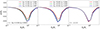 |
Fig. 4. Void-lensing signals in different cosmologies and different galaxy population processes. The x-axis represents the projection radius rescaled by the void radius. The y-axis is the excess surface density (ESD) around voids. These are the data vectors used by SBI. |
5.2. Predictions of different cosmology
We first validate if the predicted mean values of parameters are unbiased in different cosmologies and if the estimated uncertainties are neither overconfident nor underconfident. For the former, we directly compared the SBI predictions of the model parameters and the truth; for the latter, the TARP metric was applied to evaluate the accuracy of our posterior, especially the estimation of the uncertainty. As is discussed in Sect. 4, 1000 samples were prepared for the validation, with 100 of them having independent cosmological parameters.
Figure 5 shows the predicted mean values as a function of the truths for all the cosmological parameters and HAM parameters. The x-axis represents the true value and the y-axis is the predicted value. For cosmological parameters, our estimator can give unbiased predictions for all of the validation samples. However, for the HAM parameter, especially for the larger values (σ>2.5), the predictions are not entirely accurate. This may be due to the fact that void-lensing signals show less response for the larger σ, but may also imply that σ is not well trained resulting from the low sampling density for σ parameter (10 samples in [0,5] for one cosmology). Since, in real observation, low-redshift galaxy samples prefer a small value of σ (σ<1), it is not a severe problem in real-world applications. In addition, in this work we are only interested in the cosmological parameters and we treat the galaxy-halo connection parameter as a nuisance parameter to be marginalized over. Due to the weak degeneracy between HAM and cosmological parameters (see Fig. 8), we do not expect the constraints on the cosmology to be greatly influenced.
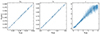 |
Fig. 5. Predicted mean values versus the truths of cosmological parameters ΩM and S8, and HAM parameter, σ, over 1000 validation sets for each parameter. The blue sticks represent 1σ regions of predictions. |
The accuracy of the predictions of cosmological parameters is shown in Fig. 6. We calculate the differences between predicted values and truths relative to their 1σ uncertainties, ΔX/σX, where X=ΩM,S8, and we give the distributions of these values. As shown in Fig. 6, we found the 1D distributions (blue histograms) for both cosmological parameters to be consistent with the standard normal distribution (orange line). These two tests confirm that for cosmological parameters drawn from the prior distribution of the training set, SBI provides unbiased predictions.
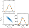 |
Fig. 6. Differences between predicted values and truths (blue dots), shown in ΩM−S8 plane. The red star represents the truth. We also present the corresponding 1D distribution of the two cosmological parameters, as well as a reference standard normal distribution (orange line). It can be seen that they are greatly consistent. |
Besides, the accuracy of the uncertainties estimated by SBI is also tested by the TARP metric, and the result is established in Fig. 7. The blue line represents the expected coverage probability (ECP) given the credibility level of 1−α. If the density estimator is accurate, namely, the estimation of the uncertainties is neither underconfident nor overconfident, ECP should be equal to 1−α; the blue line should be along with the diagonal (black dashed line). If uncertainties are overestimated (i.e., underconfident), the TARP regions from randomly selected points are more likely to cover approximately half of the posterior estimator, α∼0.5 (Lemos et al. 2023b), resulting in a “S” type curve. The light and dark shaded region of the TARP lines shows the 1σ and 2σ confidential region, which is generated by 100 bootstrap samples of the validation sets. It shows that we have obtained a highly accurate estimation of the uncertainties. A potential bias of the uncertainty estimation is barely evident, compared to the statistical fluctuations of the TARP metric.
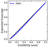 |
Fig. 7. ECP versus credibility level in TARP. The dark blue region indicates 1−σ credible region from the bootstrapping technique from 100 realizations, while the light region indicates 2−σ. If the uncertainties estimated from the posterior are accurate, the blue line should be along with the diagonal. |
Through these two validations, we can conclude that we obtain an unbiased amortized posterior estimator (i.e., SBI works on any cosmology with parameters drawn from the prior) and accurate uncertainties. These results support the accessibility of applying SBI on cosmological inference by void lensing.
5.3. Validations on multiple realizations of fiducial cosmology
In this step, we are interested in the validation of SBI on a specific cosmology sample. We ran a fiducial simulation with ΩM = 0.3156 and σ8 = 0.831, and set the HAM parameter as σ = 1.5. After obtaining the void-lensing signals following the same forward modeling process described in Sect. 3, we applied SBI to it and obtained the predictions for these parameters.
Figure 8 displays the constraining results as the 2D joint distributions of each pair of parameter set {ΩM,S8,σ} as well as the 1D marginalized distributions. The gray-dashed line represents the true value. The 68% (1σ) and 95% (2σ) credible regions are also presented in the figure with dark and light shadows. It shows that for all of the parameters, SBI can give unbiased predictions. The largest discrepancies for the two cosmological parameters are within 1σ in this single realization.
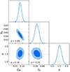 |
Fig. 8. Posterior prediction from SBI on data vector of fiducial cosmology. The thin gray lines mark the true value and 1−σ and 2−σ regions are presented as dark and light shadows. We also mark the correlation coefficients between each pair of parameters. |
To figure out if whether this discrepancy results from statistical fluctuations, we further ran 200 simulations with the same cosmological parameter, but different initial conditions and apply SBI on these lensing signals. We then averaged these signals and obtain a signal with less cosmic variance. It is expected that if SBI is unbiased, it can give a more accurate prediction on this cosmic variance-reduced sample. In Fig. 9, we illustrate the SBI prediction on the mean signal in solid filled contour, as well as predictions on four randomly chosen samples in dash empty contours. The predicted mean values for each individual sample vary around the true values, while the predictions of the mean signal are in good agreement with the true values, illustrating the fact that SBI can provide an unbiased prediction on fiducial cosmology.
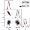 |
Fig. 9. Same as Fig. 8, but for different realizations. The red, blue, green, and magenta thin contours are the predictions of four realizations randomly chosen in the validation set. The black thick contour represents the prediction of the data vector averaged over all 200 validation samples. |
Furthermore, we checked the distribution of SBI predictions on these 200 realizations. In Fig. 10, we show the histogram of the differences between the predictions and the truths, ΔX=Xpred−Xtrue, normalized by the predicted standard deviation σX (where X=ΩM,S8 or σ) for three parameters. For comparison, we also plot the standard normal distribution in the orange line and a normal distribution shifted by the mean of the predictions from SBI in the blue line. In this figure, we do not see systematic biases for any of the parameters. Both of these two tests indicate that SBI predictions on fiducial cosmology are unbiased and the discrepancy seen in Fig. 8 results from the statistical fluctuations.
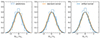 |
Fig. 10. Distributions of SBI predictions on fiducial cosmology. For each panel, the blue histogram shows the distribution of the differences between predictions and truths, rescaled by the predicted standard deviation. The orange line represents the standard normal distribution and the blue curve represents the normal distribution whose mean equals to the average of predictions. |
Regarding the degeneracy of parameters, as depicted in Fig. 8, we calculated the correlation coefficients for each pair of three parameters. This indicates that ΩM is strongly anticorrelated to S8 (ρ=−0.85), suggesting that choosing S8 to replace σ8 in our analysis does not alleviate the degeneracy between the matter density and the standard deviation of fluctuations of dark matter field. This may be expected due to the nature of lensing statistics. It can also be noticed that the degeneracy between HAM parameter σ and the other two cosmological parameters is weaker (|ρ|<0.25). It is known that the galaxy-halo connection should always be considered in cosmological analysis based on galaxy statistics and, in our case, we find that considering the galaxy-halo connection does not reduce much constraining power of void lensing on cosmology.
5.4. Influence of the shape noise
Previous results and discussions do not consider any observational uncertainties in our data vector. Therefore, the uncertainties of our predictions are purely from cosmic variance and neural network uncertainties. When including observational systematics, the constraining power and degeneracy between model parameters may be changed. In this section, we describe how we made a preliminary consideration of the effects of shape noise on our results, which is a typical source of uncertainties in weak lensing surveys.
A direct and accurate estimation of shape noise requires a ray-tracing simulation. Due to the limitation of time and computational resources, we only ran one ray-tracing simulation at fiducial cosmology to estimate the covariance and assume the covariance is independent on cosmology. We first ran FastPM with the same configuration as used in generating training sets, but saved the full sky lightcone particles from z = 1 to z = 0. Then we construct the discrete matter fields by mapping lightcone particles to healpix maps with Nside = 1024. In total 40 mass maps are constructed from z = 0 to z = 1 with interval δz = 0.025. Then we use the public ray-tracing code DORIAN10 (Ferlito et al. 2024) to obtain the background convergence and shear fields. Then, we cut a continuous sky region with area A∼1000 deg2. Shape noise is controlled by two factors: galaxy number density, ngeff, and ellipticity dispersion, σe. For the former, we chose two values: ngeff = 6 arcmin−2 and ngeff = 20 arcmin−2, which match the stage-III and stage-IV weak-lensing survey, respectively. For the latter, we chose σe = 0.288. The shape noise can be introduced by adding a noise shear, n=n1+in2, to the shear, γ=γ1+iγ2, to obtain the measured ellipticity, e=e1+ie2: e=(γ+n)/(1+γn*), where n1 and n2 are sampled from Gaussian distribution  . Finally, we can measure the void-shear cross correlation using the following estimator:
 (8)
(8)
We can use the jackknife technique to estimate the covariance matrix. Here, njk = 32 subsamples were used in the covariance estimation. In addition, for the stage-IV survey, we also consider the influence of the sky coverage by rescaling the covariance matrix with respect to the survey area.
With the covariance in hand, we can generate a set of data vectors, whose means are equal to the noise-free values and whose covariance equals what we obtained before. We trained our SBI networks using these data vectors as training sets to estimate the posteriors. The network architecture is almost the same as in analyzing noise-free data, but we adjusted the learning rate to be 0.0001 and batch size to 128 to obtain a better performance. We used a full-connection network to first compress the data vectors to eight dimensions to suppress the noise. Our results are shown in Fig. 11.
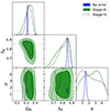 |
Fig. 11. Constraining results after considering two kinds of shape noise: one matches the stage-III survey (shown in green filled contour) and the other matches stage-IV (shown in black dashed contour). The noise-free case is shown in blue contour. |
It is obvious that even if we update our neural network, considering the shape noise still greatly degrades the constraining power of void lensing. The posteriors of all three parameters are almost similar to the priors, especially for the HAM parameter. Reducing the shape noise level from stage-III to stage-IV case can increase the constraining power on cosmological parameters, but not for HAM parameters. These results, on the one hand, illustrate that our noise-free void-lensing model is accurate enough (the model uncertainties shown in the blue contour are negligible compared to stage-IV level shape noise shown in the black dashed contour). On the other hand, they illustrate that the data processing and neural network architecture need to be optimized to extract more information from void-lensing. In future works, some points could be investigated: the optimized void size bins; tomography (i.e., considering combinations between multiple redshift bins); data compression – for instance, by using a principle component analysis, PCA, or including embedding nets in the SBI inference process to reduce the dimensionality of the data and to suppress the influence of the statistical noise.
6. Summary and conclusion
Void statistics are expected to offer more cosmological information than we are able to obtain from two-point statistics. In this work, we applied the simulation-based inference (SBI) method on void lensing to set constraints on cosmological parameters. Instead of building an explicit likelihood function, we constructed a neural network to learn the posterior directly from a set of simulated data. With this method, we avoided the challenging task of explicitly modeling the likelihood of void-lensing statistics.
The aim of this work is to explore the potential of constraining cosmological parameters using void lensing with SBI. We show that SBI can recover a posterior distribution with unbiased mean values and slightly overestimated uncertainty. In particular, both cosmological and galaxy formation effects are incorporated into the inference pipeline. Furthermore, the final posterior can at least provide unbiased predictions of cosmological parameters, ΩM and S8, across different cosmologies. This is an encouraging result and in the future, both the forward modeling process and the inference process will be developed to analyze the real observational data. In this work we have achieved the following goals:
-
(1)
We used the novel method, SBI, to study the accessibility and performance of void lensing on setting cosmological constraints. We show that by use of SBI, we achieve the Bayesian inference without an explicit likelihood and successfully recover the input model parameters. Therefore, with the help of SBI, we can overcome the problem of the absence of void-lensing models and make it possible to use void lensing to constrain cosmology. Besides, SBI also has the following two advantages. First, it does not assume a Gaussian likelihood as traditional Bayesian analysis, which may capture more information from high-order statistics or statistics containing non-Gaussian information (also, the predicted likelihood should be carefully validated). Second, in this work, we used the NPE framework, which does not need MCMC sampling, thus making this approach quite computationally efficient. We also point out that the SBI pipeline used in this work can also be easily applied to other complicated statistics that are difficult to model.
-
(2)
We constructed a complete forward modeling pipeline to simulate void-lensing signal beginning from cosmological parameters. We discover that for void-lensing statistics, two cosmological parameters, ΩM and S8, are degenerate, while the HAM parameter σ does not degenerate with the other two. However, we point out that in any case both the cosmology and the galaxy formation process should be taken into account in the forward modeling process. In addition to cosmology, the galaxy formation process can also affect galaxy-based statistics and incomplete modeling of galaxy-halo connections may potentially lead to a biased inference. We believe that considering the galaxy-halo connection is a crucial step in applying our method to real data.
-
(3)
We present thorough validation tests to confirm results obtained from SBI. The validation of predictions is one of the most important parts of every ML application literature. Multiples of validation methods have been presented in recent years and been applied in relevant papers. In this work, apart from some popular mathematical validation tests (e.g., TARP), we also carefully validated the SBI results on realizations of a single simulation. Thus, we were able to alleviate the influence of cosmic variance. In other words, even SBI can predict biased results on one single realization, but it gives an unbiased prediction when averaging a large number of realizations. This validation test is more intuitive and can strongly imply the accuracy of SBI predictions.
-
(4)
We preliminarily investigated the effects from shape noise on our SBI results and we find that shape noise contaminates the void-lensing signals and prevents us from setting constraints as strong as in the noise-free case. To extract more cosmological information from noisy lensing signals, it is necessary to develop both the data preprocessing method and the neural network to learn a more accurate posterior. To apply our method to real data, in future works, we plan to consider the following points more carefully.
-
(1)
Necessity of light-cone simulations: with the light-cone, we can use the ray-tracing method to obtain a synthesis shear catalog and one measure the lensing signals in the same way as in real data. Furthermore, it is also convenient to consider the statistical error and systematics in shear measurements and redshift measurements. All of these reasons motivated us to run light-cone simulation in the next step.
-
(2)
Systematics: in modern cosmological analysis, a careful consideration of the systematics is of great importance because an insufficient modeling of systematics will lead to biased inference of the cosmological parameters. In SBI, this is also a key point since all of the information of the posterior comes from the simulated data and if the simulated data do not contain systematics, SBI could end up learning inaccurate relations between data and parameters, potentially leading to biased inferences when applied to real data. Therefore, in future works, if we want to apply SBI to real data, we must include as much known systematics in our forward modeling as possible.
-
(3)
Accuracy of simulations: all the results in this work are derived in a self-consistent way; namely, the training set and the validation set come from the same forward modeling procedure and the conclusion is that it is possible to apply SBI on void lensing to extract cosmological information. In the future, we plan to further test the accuracy of our fast simulation as well as the halo-galaxy connection; namely, to consider whether the results training on fast simulation is suitable for observables from high-fidelity simulation and how the training results changes if the galaxy-halo connection is changed (e.g., from HAM to HOD). In addition, we notice that Jia (2024) presents a hybrid training strategy that uses large fast simulations as a training set and small high-accuracy simulations to calibrate the training results, which can significantly reduce the computational cost and maintain high prediction accuracy. This is a valuable reference and in future work, we plan to introduce this strategy in our method and investigate the performance.
Recent developments in the observational data highlight the need to improve the data analysis. To maximize the extraction of information from these data, it is essential to identify statistics that preserve as much cosmological information as possible. Void statistics is one such method, as it is expected to capture information from galaxy N-point statistics. The endpoint of this approach might be field-level inference, since at a fixed resolution, the field includes the full cosmological information. Modeling statistics that contain more information is typically more challenging and the likelihood might not follow a Gaussian distribution. Therefore, ML techniques, such as SBI used in this work, could be helpful. Combining ML with high-order statistics could tighten constraints on the cosmological model and bring us toward a deeper understanding of our Universe.
Acknowledgments
We acknowledge the support by the Ministry of Science and Technology of China (grant Nos. 2020SKA0110100) and National Key R&D Program of China No. 2022YFF0503403. CS would like to thank Mingshan Xie, Linfeng Xiao for valuable discussions and suggestions on this work. CS would also like to thank “Tree New Bee” club for supporting friendly discussion environment. HYS acknowledges the support from NSFC of China under grant 11973070, Key Research Program of Frontier Sciences, CAS, Grant No. ZDBS-LY-7013 and Program of Shanghai Academic/Technology Research Leader. CZ acknowledges the support from National Key R&D Program of China (grant No. 2023YFA1605600). We acknowledge the support from the science research grants from the China Manned Space Project with NO. CMS-CSST-2021-A01, CMS-CSST-2021-A04.
In Bonici et al. (2023), a model with a linear void bias was built to describe the void-matter cross power spectrum, but it is known that void bias is scale-dependent and has an oscillation feature on the high k end due to void exclusion effects (Zhao et al. 2016; Chan et al. 2014).
Which is also called the implicit likelihood inference (ILI) and likelihood-free inference (LFI).
“Density” means it estimates a probability density function rather than some deterministic values.
According to the maximum-likelihood estimation principle, these parameters should be chosen when the value of qϕ(θ|d) is maximum in each of the observation, di, which is the theoretical support of the training strategy.
References
- Aihara, H., Armstrong, R., Bickerton, S., et al. 2017, PASJ, 70, S8 [Google Scholar]
- Asgari, M., Lin, C. A., Joachimi, B., et al. 2021, A&A, 645, A104 [NASA ADS] [CrossRef] [EDP Sciences] [Google Scholar]
- Bayer, A. E., Villaescusa-Navarro, F., Massara, E., et al. 2021, ApJ, 919, 24 [NASA ADS] [CrossRef] [Google Scholar]
- Bechtol, K., Sevilla-Noarbe, I., Drlica-Wagner, A., et al. 2025, arXiv e-prints [arXiv:2501.05739] [Google Scholar]
- Behroozi, P. S., Wechsler, R. H., & Wu, H. -Y. 2012, ApJ, 762, 109 [Google Scholar]
- Bonici, M., Carbone, C., Davini, S., et al. 2023, A&A, 670, A47 [NASA ADS] [CrossRef] [EDP Sciences] [Google Scholar]
- Boschetti, R., Vielzeuf, P., Cousinou, M. -C., Escoffier, S., & Jullo, E. 2024, JCAP, 2024, 067 [CrossRef] [Google Scholar]
- Burger, P. A., Friedrich, O., Harnois-Déraps, J., et al. 2023, A&A, 669, A69 [NASA ADS] [CrossRef] [EDP Sciences] [Google Scholar]
- Cai, Y. -C., Padilla, N., & Li, B. 2015, MNRAS, 451, 1036 [NASA ADS] [CrossRef] [Google Scholar]
- Chan, K. C., Hamaus, N., & Desjacques, V. 2014, Phys. Rev. D, 90, 103521 [NASA ADS] [CrossRef] [Google Scholar]
- Chantavat, T., Sawangwit, U., Sutter, P. M., & Wandelt, B. D. 2016, Phys. Rev. D, 93, 043523 [NASA ADS] [CrossRef] [Google Scholar]
- Chantavat, T., Sawangwit, U., & Wandelt, B. D. 2017, ApJ, 836, 156 [NASA ADS] [CrossRef] [Google Scholar]
- Cheng, S., Marques, G. A., Grandón, D., et al. 2024, arXiv e-prints [arXiv:2404.16085] [Google Scholar]
- Dawson, K. S., Schlegel, D. J., Ahn, C. P., et al. 2012, AJ, 145, 10 [Google Scholar]
- DESI Collaboration (Aghamousa, A., et al.) 2016a, arXiv e-prints [arXiv:1611.00036] [Google Scholar]
- DESI Collaboration (Aghamousa, A., et al.) 2016b, arXiv e-prints [arXiv:1611.00037] [Google Scholar]
- DESI Collaboration (Karim, M. A., et al.) 2025, arXiv e-prints [arXiv:2503.14738] [Google Scholar]
- Eisenstein, D. J., Weinberg, D. H., Agol, E., et al. 2011, AJ, 142, 72 [Google Scholar]
- Feng, Y., Chu, M. -Y., Seljak, U., & McDonald, P. 2016, MNRAS, 463, 2273 [NASA ADS] [CrossRef] [Google Scholar]
- Ferlito, F., Davies, C. T., Springel, V., et al. 2024, MNRAS, 533, 3209 [Google Scholar]
- Gil-Marín, H., Verde, L., Noreña, J., et al. 2015, MNRAS, 452, 1914 [Google Scholar]
- Gong, Y., Liu, X., Cao, Y., et al. 2019, ApJ, 883, 203 [NASA ADS] [CrossRef] [Google Scholar]
- Hahn, C., Eickenberg, M., Ho, S., et al. 2023a, Proc. Natl. Acad. Sci., 120, e2218810120 [Google Scholar]
- Hahn, C., Eickenberg, M., Ho, S., et al. 2023b, JCAP, 2023, 010 [CrossRef] [Google Scholar]
- Hahn, C., Eickenberg, M., Ho, S., et al. 2023c, PRD, submitted [arXiv:2310.15243] [Google Scholar]
- Hahn, C., Lemos, P., Parker, L., et al. 2024, Nat. Astron., 8, 1457 [Google Scholar]
- Halder, A., Gong, Z., Barreira, A., et al. 2023, JCAP, 2023, 028 [CrossRef] [Google Scholar]
- Harnois-Déraps, J., Martinet, N., Castro, T., et al. 2021, MNRAS, 506, 1623 [CrossRef] [Google Scholar]
- Heydenreich, S., Brück, B., & Harnois-Déraps, J. 2021, A&A, 648, A74 [NASA ADS] [CrossRef] [EDP Sciences] [Google Scholar]
- Heymans, C., Tröster, T., Asgari, M., et al. 2021, A&A, 646, A140 [NASA ADS] [CrossRef] [EDP Sciences] [Google Scholar]
- Ho, M., Bartlett, D. J., Chartier, N., et al. 2024, Open J. Astrophys., 7, 54 [NASA ADS] [CrossRef] [Google Scholar]
- Hou, J., Dizgah, A. M., Hahn, C., et al. 2024, arXiv e-prints [arXiv:2401.15074] [Google Scholar]
- Ivanov, M. M., Philcox, O. H. E., Cabass, G., et al. 2023, Phys. Rev. D, 107, 083515 [NASA ADS] [CrossRef] [Google Scholar]
- Jeffrey, N., Whiteway, L., Gatti, M., et al. 2024, MNRAS, 536, 1303 [NASA ADS] [CrossRef] [Google Scholar]
- Jia, H. 2024, arXiv e-prints [arXiv:2411.14748] [Google Scholar]
- Kreisch, C. D., Pisani, A., Villaescusa-Navarro, F., et al. 2022, ApJ, 935, 100 [NASA ADS] [CrossRef] [Google Scholar]
- Lai, L., Ding, J., Luo, X., et al. 2024, Sci. China Phys., Mech. Astron., 67, 289512 [Google Scholar]
- Laureijs, R., Amiaux, J., Arduini, S., et al. 2011, arXiv e-prints [arXiv:1110.3193] [Google Scholar]
- Lemos, P., Parker, L., Hahn, C., et al. 2023a, arXiv e-prints [arXiv:2310.15256] [Google Scholar]
- Lemos, P., Coogan, A., Hezaveh, Y., & Perreault-Levasseur, L. 2023b, in Proceedings of the 40th International Conference on Machine Learning, eds. A. Krause, E. Brunskill, K. Cho, et al., Proceedings of Machine Learning Research, 202 [Google Scholar]
- LSST Science Collaboration (Abell, P. A., et al.) 2009, arXiv e-prints [arXiv:0912.0201] [Google Scholar]
- Massara, E., Villaescusa-Navarro, F., Viel, M., & Sutter, P. 2015, JCAP, 2015, 018 [Google Scholar]
- Massara, E., Hahn, C., Eickenberg, M., et al. 2024, arXiv e-prints [arXiv:2404.04228] [Google Scholar]
- Novaes, C. P., Thiele, L., Armijo, J., et al. 2024, arXiv e-prints [arXiv:2310.15256] [Google Scholar]
- Pisani, A., Massara, E., Spergel, D. N., et al. 2019, arXiv e-prints [arXiv:1903.05161] [Google Scholar]
- Poh, J., Samudre, A., Ćiprijanović, A., et al. 2022, arXiv e-prints [arXiv:2211.05836] [Google Scholar]
- Régaldo-Saint Blancard, B., Hahn, C., Ho, S., et al. 2024, Phys. Rev. D, 109, 083535 [CrossRef] [Google Scholar]
- Rodríguez-Torres, S. A., Chuang, C. -H., Prada, F., et al. 2016, MNRAS, 460, 1173 [CrossRef] [Google Scholar]
- Singh, S., Mandelbaum, R., Seljak, U., Rodríguez-Torres, S., & Slosar, A. 2019, MNRAS, 491, 51 [Google Scholar]
- Steinmetz, M., & Navarro, J. F. 1999, ApJ, 513, 555 [CrossRef] [Google Scholar]
- Su, C., Shan, H., Zhang, J., et al. 2023, ApJ, 951, 64 [Google Scholar]
- Tasitsiomi, A., Kravtsov, A. V., Wechsler, R. H., & Primack, J. R. 2004, ApJ, 614, 533 [NASA ADS] [CrossRef] [Google Scholar]
- Thiele, L., Massara, E., Pisani, A., et al. 2024, ApJ, 969, 89 [NASA ADS] [CrossRef] [Google Scholar]
- von Wietersheim-Kramsta, M., Lin, K., Tessore, N., et al. 2025, A&A, 694, A223 [NASA ADS] [CrossRef] [EDP Sciences] [Google Scholar]
- Wenzl, L., An, R., Battaglia, N., et al. 2024, PRD, accepted [arXiv:2405.12795] [Google Scholar]
- Willick, J. A., Courteau, S., Faber, S. M., et al. 1997, ApJS, 109, 333 [NASA ADS] [CrossRef] [Google Scholar]
- Wilson, C., & Bean, R. 2021, Phys. Rev. D, 104, 023512 [NASA ADS] [CrossRef] [Google Scholar]
- Wright, A. H., Stölzner, B., Asgari, M., et al. 2025, A&A, submitted [arXiv:2503.19441] [Google Scholar]
- Yao, J., Shan, H., Zhang, P., et al. 2023, A&A, 673, A111 [NASA ADS] [CrossRef] [EDP Sciences] [Google Scholar]
- Yu, J., Zhao, C., Chuang, C. -H., et al. 2022, MNRAS, 516, 57 [Google Scholar]
- Yu, J., Zhao, C., Gonzalez-Perez, V., et al. 2023, MNRAS, 527, 6950 [CrossRef] [Google Scholar]
- Zhan, H. 2021, Chin. Sci. Bull., 66, 1290 [CrossRef] [Google Scholar]
- Zhao, C. 2023, A&A, 672, A83 [NASA ADS] [CrossRef] [EDP Sciences] [Google Scholar]
- Zhao, C., Tao, C., Liang, Y., Kitaura, F. -S., & Chuang, C. -H. 2016, MNRAS, 459, 2670 [NASA ADS] [CrossRef] [Google Scholar]
- Zhao, X., Mao, Y., & Wandelt, B. D. 2022, ApJ, 933, 236 [NASA ADS] [CrossRef] [Google Scholar]
- Zhao, C., Huang, S., He, M., et al. 2024, SCPMA, submitted [arXiv:2411.07970] [Google Scholar]
All Figures
|
Fig. 1. Workflow of a typical SBI with neural posterior estimation (NPE), i.e., directly estimating the posterior. The forward modeling process transforms parameters to be inferred to data vector, and therefore includes the process of measuring summary statistics from simulation results in our case. The density estimator takes parameter-data pair {θ,d} as input, and after the training procedure returns an estimation of posterior. Note: for the neural likelihood estimation (NLE) and neural ratio estimation (NRE), the target to be trained (shown in green block) is the likelihood and the ratio of likelihood and prior, respectively. Combined with the prior, this allows us to easily build the posterior using Bayes law. |
| In the text | |
|
Fig. 2. Schematic diagram of forward modeling. The gray blocks represent modeling processes, the green blocks represent outputs in each step of modeling. The red block represents input parameters in the model. The gray blocks represent steps in forward modeling and the green blocks show the corresponding output in each step. The final output i.e., the void-lensing signal is shown in blue. |
| In the text | |
|
Fig. 3. Parameter space of parameters considered in this work, including cosmological parameters ΩM, S8, and HAM parameter, σ. These samples are randomly divided into two parts with 9:1, corresponding to the training set (orange dots) and validation set (blue dots), respectively. To test the performance of our method on a special cosmology, we chose a fiducial cosmology marked as red star. Note: this sample is neither in the training set, nor the validation set. |
| In the text | |
|
Fig. 4. Void-lensing signals in different cosmologies and different galaxy population processes. The x-axis represents the projection radius rescaled by the void radius. The y-axis is the excess surface density (ESD) around voids. These are the data vectors used by SBI. |
| In the text | |
|
Fig. 5. Predicted mean values versus the truths of cosmological parameters ΩM and S8, and HAM parameter, σ, over 1000 validation sets for each parameter. The blue sticks represent 1σ regions of predictions. |
| In the text | |
|
Fig. 6. Differences between predicted values and truths (blue dots), shown in ΩM−S8 plane. The red star represents the truth. We also present the corresponding 1D distribution of the two cosmological parameters, as well as a reference standard normal distribution (orange line). It can be seen that they are greatly consistent. |
| In the text | |
|
Fig. 7. ECP versus credibility level in TARP. The dark blue region indicates 1−σ credible region from the bootstrapping technique from 100 realizations, while the light region indicates 2−σ. If the uncertainties estimated from the posterior are accurate, the blue line should be along with the diagonal. |
| In the text | |
|
Fig. 8. Posterior prediction from SBI on data vector of fiducial cosmology. The thin gray lines mark the true value and 1−σ and 2−σ regions are presented as dark and light shadows. We also mark the correlation coefficients between each pair of parameters. |
| In the text | |
|
Fig. 9. Same as Fig. 8, but for different realizations. The red, blue, green, and magenta thin contours are the predictions of four realizations randomly chosen in the validation set. The black thick contour represents the prediction of the data vector averaged over all 200 validation samples. |
| In the text | |
|
Fig. 10. Distributions of SBI predictions on fiducial cosmology. For each panel, the blue histogram shows the distribution of the differences between predictions and truths, rescaled by the predicted standard deviation. The orange line represents the standard normal distribution and the blue curve represents the normal distribution whose mean equals to the average of predictions. |
| In the text | |
|
Fig. 11. Constraining results after considering two kinds of shape noise: one matches the stage-III survey (shown in green filled contour) and the other matches stage-IV (shown in black dashed contour). The noise-free case is shown in blue contour. |
| In the text | |
Current usage metrics show cumulative count of Article Views (full-text article views including HTML views, PDF and ePub downloads, according to the available data) and Abstracts Views on Vision4Press platform.
Data correspond to usage on the plateform after 2015. The current usage metrics is available 48-96 hours after online publication and is updated daily on week days.
Initial download of the metrics may take a while.