| Issue |
A&A
Volume 696, April 2025
|
|
|---|---|---|
| Article Number | A183 | |
| Number of page(s) | 9 | |
| Section | Cosmology (including clusters of galaxies) | |
| DOI | https://doi.org/10.1051/0004-6361/202452174 | |
| Published online | 17 April 2025 | |
An emulation-based model for the projected correlation function
Institute of Theoretical Astrophysics, University of Oslo, 0315 Oslo, Norway
⋆ Corresponding author; This email address is being protected from spambots. You need JavaScript enabled to view it.
Received:
8
September
2024
Accepted:
17
March
2025
Abstract
Data from the ongoing Euclid survey will map out billions of galaxies in the Universe, covering more than a third of the sky. This data will provide a wealth of information about the large-scale structure of the Universe and will have a significant impact on cosmology in the coming years. In this paper we introduce an emulator-based halo model approach to forward-modeling the relationship between cosmological parameters and the projected galaxy-galaxy two-point correlation function (2PCF). Utilizing the large ABACUSSUMMIT simulation suite, we emulated the 2PCF by generating mock-galaxy catalogs within the halo occupation distribution (HOD) framework. Our emulator is designed to predict the 2PCF over scales 0.1 ≤ r/(h−1 Mpc)≤105, from which we derived the projected correlation function, independent of redshift space distortions. We demonstrate that the emulator accurately predicts the projected correlation function over scales 0.5 ≤ r⊥/(h−1 Mpc)≤40 given a set of cosmological and HOD parameters. We then employed this model in a parameter inference analysis, showcasing its ability to constrain cosmological parameters. Our findings indicate that the projected correlation function places only weak constraints on several cosmological parameters due to its intrinsic lack of information; additional clustering statistics are necessary to better probe the underlying cosmology. Despite the simplified covariance matrix used in the likelihood model, the posterior distributions of several cosmological parameters remain broad, underscoring the need for a more comprehensive approach.
Key words: large-scale structure of Universe
© The Authors 2025
 Open Access article, published by EDP Sciences, under the terms of the Creative Commons Attribution License (https://creativecommons.org/licenses/by/4.0), which permits unrestricted use, distribution, and reproduction in any medium, provided the original work is properly cited.
This article is published in open access under the Subscribe to Open model. This email address is being protected from spambots. You need JavaScript enabled to view it. to support open access publication.
1. Introduction
Modern galaxy redshift surveys, such as the Sloan Digital Sky Survey (SDSS; York et al. 2000), Two Degree Field Galaxy Redshift Survey (2dFGRS; Colless et al. 2001; Cole et al. 2005), WiggleZ Dark Energy Survey (Drinkwater et al. 2010), Baryon Oscillation Spectroscopic Survey (BOSS; Dawson et al. 2013, 2016; Alam et al. 2021), Dark Energy Spectroscopic Instrument (DESI; DESI Collaboration 2016), and Euclid (Laureijs et al. 2011), have enabled us to study the large-scale structure of the Universe, which is mainly traced by galaxies. To fully exploit the next generation of observational data, we need accurate models of galaxy clustering.
In typical galaxy surveys, measurements of clustering statistics, such as the two-point correlation function (2PCF), are more precise at megaparsec scales, which is below the valid scales of state-of-the-art perturbation theory approaches. The fully nonlinear treatment, N-body simulations, is essential for accurately resolving the nonlinear dynamics in structure formation. However, simulations are computationally demanding, posing a significant bottleneck in the exploration of cosmological parameter space.
In contemporary galaxy formation and evolution theories, galaxies form and evolve in dark matter halos. After the distribution of halos is obtained from simulations, we adopt the framework of halo occupation distribution (HOD; Peacock & Smith 2000; Seljak 2000; Berlind & Weinberg 2002; Zheng et al. 2005; Guo et al. 2014) as the galaxy-halo connection model. HOD models have been widely applied to interpret galaxy clustering data (e.g., Zheng et al. 2009; Guo et al. 2015; Zentner et al. 2019). In its basic form, the HOD quantifies the likelihood, P(N|M), that a dark matter halo of mass M contains N galaxies. Together with models of the spatial and velocity distributions of galaxies inside halos, the HOD framework can interpret the clustering of galaxies down to nonlinear scales.
Given the computational requirements of N-body simulations and advancements in machine learning techniques in recent years, emulators have emerged as an increasingly popular tool for modeling galaxy clustering statistics within the HOD framework (e.g., Kwan et al. 2015; Kobayashi et al. 2022; Nishimichi et al. 2019; Zhai et al. 2019, 2023; Kwan et al. 2023; Cuesta-Lazaro et al. 2023, 2024; Burger et al. 2024; Storey-Fisher et al. 2024). The core idea of emulators is to evenly sample the parameter space and apply novel interpolation schemes to create high-accuracy estimates of clustering statistics at any point within that space. We have built a model based on the ABACUSSUMMIT simulations (Maksimova et al. 2021).
The radial positions of galaxies are usually derived from the observed galaxy redshifts assuming a cosmological model. However, these derived distances differ from the true positions due to peculiar velocities, an effect known as redshift-space distortions (RSDs). A traditional way to probe the real-space galaxy clustering and mitigate the RSD effect is through the projected 2PCF, wp(r⊥), obtained by integrating the three-dimensional 2PCF, ξS(r⊥, r∥), along the line-of-sight (LOS; r∥) direction. In this work, we limit our attention to the real-space galaxy 2PCF, ξR(r), building emulators for it and demonstrating that the emulators can recover unbiased cosmological constraints in a likelihood analysis. The modeling of redshift-space clustering will be presented in subsequent studies, where the emulators for ξR(r) will serve as one of the model ingredients.
The structure of this paper is as follows: In Sect. 2 we introduce the theoretical background for the galaxy clustering. In Sect. 3 we give a brief overview of the suite of cosmological N-body simulations used in this work and outline how we constructed galaxy catalogs from them. In Sect. 4 we present our neural network emulator. Then, we present our method for recovering cosmological parameters in Sect. 5, before presenting the results in Sect. 6. Finally, we discuss our results in Sect. 7 before concluding in Sect. 8.
2. Theoretical background
The spatial distribution of galaxies can be quantified in terms of the 2PCF, ξgg(r), which measures the excess probability of finding a pair of galaxies at a given separation, compared to that of a random distribution. In cosmological surveys, the comoving distance to a galaxy, r(z), is inferred from its redshift via
 (1)
(1)
where H(z) is the Hubble factor. We used natural units where the speed of light is c = 1.
In addition to the Doppler shift resulting from the Universe’s expansion, light emitted from galaxies experiences an additional shift due to peculiar velocities. These peculiar velocities induce anisotropies in the measured spatial distribution of galaxies, known as RSDs. If a galaxy pair is separated by a vector r in real space, it will be separated by a vector s in redshift space. We adopted the distant-observer approximation, where galaxies are assumed to be sufficiently distant such that the angle they subtend with respect to the LOS direction, denoted by  , is negligible. Under this assumption, galaxies’ peculiar velocity only induces a redshift in the
  direction. To the linear order in velocity, |v|≪1, the redshift-space separation of galaxies due to peculiar velocities is given as
 (2)
(2)
where  is the peculiar velocity of the galaxy along the LOS, a(z) is the scale factor and H(z) the Hubble factor.
We decomposed the separation vectors r and s into a component parallel and perpendicular to the LOS, s||, r|| and s⊥, r⊥, respectively. Under the distant-observer approximation, RSD effects are isolated into s||, meaning we have r⊥ = s⊥. Consequently, projecting galaxies onto a plane orthogonal to r|| results in the same distribution of galaxies in real and redshift space, known as the projected correlation function,
 (3)
(3)
where the equality holds if πmax is sufficiently large for correlations to be negligible beyond it. We use superscript S and R to denote redshift space and real space, respectively, and  . Importantly, the projected correlation function is independent of RSD effects under the distant-observer approximation, meaning we can model ξR without having to account for peculiar velocity, which can be directly confronted with measurements from observations.
3. Constructing mock galaxy catalogs
In this section we briefly describe the N-body simulations and the catalogs of HOD galaxies used in the analyses.
3.1. The ABACUSSUMMIT simulation suite
ABACUSSUMMIT (Maksimova et al. 2021) is a suite of large, high-accuracy cosmological N-body simulations. In this work, we mainly focused on the base simulations of the suite with a volume of 2 (h−1 Gpc)3 containing 69123 with a mass resolution of 2 ⋅ 109 h−1 M⊙. The simulation suite contains 150 simulation boxes spanning 97 cosmological models. They assume a flat space-time, and the Hubble constant H0 is calibrated to match the cosmic microwave background acoustic scale θ*. The 8 varying parameters are
 (4)
(4)
where ωcdm = Ωcdmh2 and ωb = Ωbh2 are the physical cold dark matter and baryon densities, σ8 is the amplitude of the matter power spectrum, w0 is the dark energy equation of state today, wa governing the time evolution of the dark energy equation of state according to the CPL (Chevallier & Polarski 2001; Linder 2003) parameterization,
 (5)
(5)
where w0 = −1 and wa correspond to a cosmological constant, ns is the spectral tilt, dns/dlnk is the running of the spectral tilt and Neff is the effective number of neutrino species.
The base simulations considered in this paper are organized into the following subsets:
-
c000: Fiducial cosmology matching Planck 2018 (Planck Collaboration VI 2020) particularly the mean estimates of the TT,TE,EE+lowE+lensing likelihood chains. This cosmology contains 25 independent realizations, referred to as the fiducial cosmology in this paper.
-
c001-c004: Secondary cosmologies, including a low ωcdm, thawing dark energy, high Neff and low σ8.
-
c100-c126: Linear derivative grid with simulation pairs with small positive and negative steps in eight-dimensional parameter space.
-
c130-c181: Broad emulator grid, covering a wider range of the full cosmological parameter space. All simulations in this grid have the same phase seed.
Table 1 shows the fiducial value and the prior ranges of the cosmological parameters covered by the simulations.
Cosmological parameters with their fiducial values and their prior ranges.
The c001-c004 simulations contain six independent realizations each, but we limited ourselves to a single realization to reduce data storage requirements. In addition to the base simulations, we used the ABACUSSMALL simulations to estimate the covariance matrix used for parameter inference analysis in Sect. 5. These contain 1687 independent realizations of the fiducial cosmology with 17283 particles in a (0.5 h−1 Gpc)3 volume box.
The group finding in each simulation is done on the fly, using a hybrid friends-of-friends spherical overdensity (SO) algorithm named COMPASO (Hadzhiyska et al. 2021). This paper only considers halo catalogs from snapshots at a single redshift of z = 0.25. As described in Hadzhiyska et al. (2021), there are three types of halos in the simulation suite, and we limited our analysis to the main halo catalogs, named L1. The resulting catalogs are then populated by galaxies, following the procedure described in the following subsection.
3.2. Modeling the galaxy-halo connection
To construct galaxy catalogs from the ABACUS halos, we adopted the HOD model introduced by Zheng et al. (2005), where the number of galaxies in a halo is determined by the halo mass alone, meaning that we ignored galaxy assembly bias. We parametrized central galaxies according to a Bernoulli distribution and satellites according to a Poisson distribution, using functional forms that were developed to match the clustering of luminous red galaxies.
The mean occupation number of central galaxies is parametrized as
 (6)
(6)
where erf(x) is the error function, Mmin represents the typical halo mass required to host a central galaxy, and σlog M determines the width of the distribution.
The mean occupation number of satellites is given as
 (7)
(7)
where we make the common assumption that satellite galaxies only reside in halos that already contain a central galaxy. Here, κMmin is the minimum halo mass required to host a satellite galaxy, M1 can be interpreted as the typical halo mass required to host a satellite galaxy, and α is a power-law index governing the satellite occupation’s mass dependence.
Our HOD model comprises the five HOD parameters. However, we can fix one parameter via the mean galaxy number density,
![Mathematical equation: $$ \begin{aligned} \bar{n}_g = \int \mathrm{d}M \frac{\mathrm{d}n}{\mathrm{d}M} \left[\langle {N_c}\rangle (M\,|\,{\mathcal{G} }) + \langle {N_s}\rangle (M\,|\,{\mathcal{G} })\right], \end{aligned} $$](/articles/aa/full_html/2025/04/aa52174-24/aa52174-24-eq12.gif) (8)
(8)
where  is the halo mass function. Given a set of 𝒢, we can replace one HOD parameter with
  by inverting Eq. (8). Instead of Mmin, we used
  as a free parameter in our model since we have strong prior information about it from observation data. Hence, the free model parameters considered in this work is
 (9)
(9)
We emphasize that this HOD model is highly simplistic, and several extensions have been developed over the years to accurately incorporate more complex properties of galaxy-halo connection supported by modern observations (e.g., Yuan et al. 2022). Nonetheless, the base model of Zheng et al. (2005) in HOD-related analyses remains widely used and is well tested, thus serving as a natural starting point to construct an emulator-based model for predicting galaxy clustering. Importantly, two-point statistics have intrinsic information loss, and we removed RSD effects by considering the projected correlation function. The base HOD model provides a benchmark for subsequent studies with more complex HOD parameterizations when additional summary statistics are included.
We followed Cuesta-Lazaro et al. (2023) in constructing mock galaxy catalogs, adopting R200m as our halo radius definition, which is the radius of a sphere where the average enclosed density is 200 times the mean matter density of the Universe ρm0. The halo mass is given by the number of particles within the halo and is used to compute the halo radius. We note that our halo definitions deviate from those of COMPASO. In future analyses, we intend to fully integrate the COMPASO halo definitions to construct galaxy catalogs. Comparing results obtained from the two halo definitions will serve as a valuable test to determine the model independence of the results presented in this work, thereby ascertaining whether the underlying cosmology is indeed being probed.
Central galaxies are located at the host halos’ center, and satellite galaxies are distributed according to an Navarro-Frenk-White profile, uNFW(r|c(M)) (Navarro et al. 1997). For the halo concentration, c(M), we used the median concentration-mass relation from Diemer & Joyce (2019). We assumed the angular distribution of the satellite galaxies to be isotropic.
To model RSD effects, we added velocity dispersions to the populated galaxies. By assumption, central galaxies follow their host halo and are assigned their velocity. Satellite galaxies are assigned the same velocity as the host halo, with an additional offset randomly drawn from a Gaussian distribution with mean zero and a standard deviation determined by the halo’s velocity dispersion. From the velocity dispersion of galaxies we get their redshift space position according to Eq. (2).
4. Emulating the galaxy two-point correlation function
To predict the projected correlation function given a set of cosmological parameters, 𝒞 and HOD parameters, 𝒢, we constructed a neural network emulator to predict ξR(r, 𝒞, 𝒢), from which wp is obtained via Eq. (3). Emulators are computational models that efficiently approximate the behavior of a system, essentially acting as high-dimensional interpolators. In this section we describe the general setup of the neural network and its main prerequisites before introducing how mock galaxy catalogs are constructed from which the observable is computed.
To emulate the 2PCF, we employed fully connected neural networks, which approximate a function f such that
 (10)
(10)
where x represents the features of the dataset, y the target values and θ the trainable parameters of the network.
The activation function of the network is the Gaussian error linear unit (GELU; Hendrycks & Gimpel 2016), defined as
 (11)
(11)
where x is the output of the network’s previous layer, and Φ(x) is the cumulative distribution function of the standard normal distribution. The GELU activation function is a smooth approximation of the Rectified Linear Unit (ReLU) activation function (Agarap 2019). GELU exhibits more curvature and nonlinearity, which may allow it to better approximate complex functions. Another advantage is that it avoids the vanishing gradient problem.
The optimal f is defined by the set of parameters θ, which minimizes a loss function. In this work, we adapted the L1 norm
 (12)
(12)
where yitrue is the true value of the observable and yipred(θ) is the network prediction. We updated the network parameters using the Adam optimizer (Kingma & Ba 2017).
For the learning rate, we used a value of 0.01 initially and used a learning rate scheduler to reduce the learning rate by a factor of 10 if the validation loss did not improve after 20 epochs until a minimum value of 10−6 was reached. This simple scheme allows for increased training efficiency in the beginning when gradients are steep, followed by increasingly finer tuning of the parameters as the loss landscape flattens.
4.1. Training the neural network
We trained the neural network to perform the mapping:
 (13)
(13)
where 𝒞 and 𝒢 are the input parameters given in Eqs. (4) and (9), respectively, and r is the average separation distance between galaxy pairs in a given bin. Additionally, we applied standard normal scaling of the targets and features according to the transformation
 (14)
(14)
To facilitate the generalization of the network, we employed weight decay and dropout. The former reduces the weights after each iteration, preventing significant emphasis from being placed on the noise of outliers, essentially working by subtracting an L2 penalization term λ||θ||2 from Eq. (12). Dropout counteracts co-adaption, in which each network neuron depends on specific activations of other neurons, by randomly setting neurons to 0 with a probability p. Given that we have a restricted number of samples with varying cosmological parameters, dropout is an effective method for enhancing generalization (Srivastava et al. 2014). To further prevent overfitting, the training was stopped if the validation loss did not improve after 50 epochs or when a maximum of 500 epochs was reached.
4.2. Generating mock-galaxy catalogs
Our choice of fiducial HOD parameters is principally based on the analysis of Cuesta-Lazaro et al. (2023) who applied the same HOD model on the DARKQUEST simulations (Nishimichi et al. 2019) where the minimum halo mass is 1012 h−1 M⊙. In the context of these HOD parameters, ABACUS halos of mass M < 1012 h−1 M⊙ are improbable to host galaxies according to the occupation distributions in Eqs. (6) and (7). This consideration, combined with the benefits of reduced computational cost and data storage requirements of the generated mock-galaxy catalogs, prompts us to restrict our analysis to halos of mass M ≥ 1012 h−1 M⊙. There are substantial low-mass halos in the simulation suite, which means they likely contribute with additional galaxies despite have a low probabilities of hosting any. Our approach is overly simplistic, and an alternative approach to reducing the number of halo samples is to randomly down-sample halos according to a probability distribution that depends on the halo mass, as considered by Yuan et al. (2022, Eq. 13).
Instead of Mmin, we used  as a free parameter in our model since we have strong prior information about it. For the remaining HOD parameters, we adopted the fiducial values used by Cuesta-Lazaro et al. (2023, Table 3) and chose variations of ±10% as our prior ranges. Our HOD parameter’s fiducial values and prior ranges are shown in Table 2.
HOD parameters with their fiducial values and their prior ranges.
We randomly assigned 80% of the c100-c126 and c130-c180 cosmologies to the training sets and the remaining 20% to the validation sets. The c000-c004 were assigned to the test sets. Degeneracies between cosmological and HOD parameters are expected, and to break these degeneracies, we constructed numerous catalogs for each simulation. Breaking these degeneracies requires using numerous HOD parameter combinations for each cosmology. We therefore generated 500 sets of HOD parameters for the training set and 100 parameter sets each for the test and validation sets. To evenly generate samples of HOD parameters within the prior ranges in Table 2, we generated five-dimensional Latin hypercubes using the Python module SMT (Saves et al. 2024). The cosmological parameters space covered by the ABACUSBASE simulations are shown in Fig. 1.
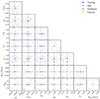 |
Fig. 1. Cosmological parameters used in the training, testing, and validation datasets. Note that the fiducial parameter values are included in the test dataset. The large number of fiducial values for some parameters is due to the linear derivative varying two parameters at a time and the fixed parameter subsets of the broad emulator grid. |
As mentioned in Sect. 3.2 we estimated the appropriate value of Mmin by inverting Eq. (8) to generate galaxy catalogs with galaxy number densities matching the desired value. From the generated galaxy catalogs, we stored the coordinates of all galaxies in real space, (x, y, z), and the redshift space coordinates sz as we isolated RSD effects to the z-axis.
4.3. Computing the 2PCF and its projection
We measured the real space 2PCF with the Python module PYCORR1, utilizing the CORRFUNC engine (Sinha & Garrison 2020; Majumdar & Arora 2019). Measurements were made using 40 logarithmically spaced separation bin edges of r ∈ [0.01, 5) h−1 Mpc and 75 linearly spaced bin edges of r ∈ [5, 150] h−1 Mpc. These bin edges are chosen to cover a range of scales, ensuring a relatively high resolution on nonlinear scales where we expected significant clustering and lower resolution on larger scales where galaxy pair counts are expected to be sparse. We retrieved the average separation distance between galaxy pairs in each bin from the measurements, which we used as input for the emulator.
Initial emulation tests revealed substantial errors in the predicted clustering on the largest and smallest scales, despite excluding samples with ξ ≤ 10−7, as shot noise was prominent. To mitigate this, we opted to restrict the analysis to samples within the range r ∈ (0.1, 105) h−1 Mpc, containing only samples with ξR(r) > 10−7.
To compute wp(r⊥) from ξR(r), we used 40 logarithmically spaced bin edges of r⊥ ∈ [0.5, 40] h−1 Mpc. Unless otherwise stated, we use this binning for all computations of wp throughout this paper. We then created a spline of ξR(r), which we integrated along r|| ∈ [0, 105] h−1 Mpc according to Eq. (3), setting ξR = 0 for values where r(r⊥, r||) extended beyond the training range considered.
5. Recovering cosmological parameters
In this section we demonstrate our emulator model’s ability to predict cosmological parameters from a mock signal of the projected correlation function. In the future, we aim to apply our model to observational data from the ongoing Euclid survey (Laureijs et al. 2011). In this work, we assessed the model’s ability to recover cosmological parameters using mock data, which provides a controlled environment for evaluating its limitations and constraining power, setting a benchmark against unknown data. Importantly, the mock data help us identify other summary statistics to incorporate into our model before applying it to real data.
We performed Markov chain Monte Carlo (MCMC) parameter inference to sample the posterior distributions in our 13-dimensional parameter space. We began by defining the posterior distribution. Up to a constant, it is given as
 (15)
(15)
where θ = {𝒞,𝒢} are the parameters we want to estimate, 𝒟 is the mock data, p(θ | 𝒟) is the posterior of the parameters given the data and p(θ) is the prior distribution of the parameters.
The likelihood function ℒ(𝒟 | 𝒞, 𝒢) describes how well our model, specified by our parameters, explains the observed data. We assumed that the likelihood follows a multivariate Gaussian distribution, as is common when retrieving cosmological parameters from galaxy clustering observables (Cuesta-Lazaro et al. 2024; Miyatake et al. 2022), and compute the log-likelihood as
![Mathematical equation: $$ \begin{aligned} \ln {\mathcal{L} }({\mathcal{D} }\,\vert \,\theta ) =&-\frac{1}{2} \sum _{r_\perp ^i,r_\perp ^j} \left[{ w}_p^\mathrm{data}(r_\perp ^i) - { w}_p(r_\perp ^i\,\vert \,\theta )\right]\nonumber \\&\times \boldsymbol{C}^{-1}\left({ w}_p^\mathrm{data}(r_\perp ^i), { w}_p^\mathrm{data}(r_\perp ^j)\right)\nonumber \\&\times \left[{ w}_p^\mathrm{data}(r_\perp ^j) - { w}_p(r_\perp ^j\,\vert \,\theta )\right]\nonumber \\&+ \mathrm{const.}, \end{aligned} $$](/articles/aa/full_html/2025/04/aa52174-24/aa52174-24-eq25.gif) (16)
(16)
where wpdata(r⊥) is the mock data vector, wp(r⊥ | θ) is the emulator’s prediction given the model parameters and C−1 is the inverse of the covariance matrix.
We used the 25 fiducial c000 simulation boxes to construct the mock data vector, using the fiducial HOD parameters listed in Table 2. We used CORRFUNC (Sinha & Garrison 2020) to estimate the projected correlation function in redshift space. The mock data signal was taken as the average wp(r⊥) from the 25 samples, shown in Fig. 2.
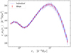 |
Fig. 2. Mock data vector wpdata(r⊥) (red) computed from averaging over the individual wp from the 25 fiducial cosmologies (blue). The error bars show the standard deviation of the individual wp samples. |
From the 25 data vector catalogs we also computed ξR over the emulator’s full separation training range, r ∈ (0.1, 105) h−1 Mpc. The average separation vector from the 25 samples as our fixed separation vector to predict ξR(r | θ) during parameter inference, from which wp(r⊥ | θ) is obtained.
We estimated the covariance matrix using the 1687 ABACUSSMALL simulation boxes, generating one mock-galaxy catalog for each box using the fiducial HOD parameters in Table 2. A cutoff mass is not considered for these simulations, as each box contains significantly fewer halos than the ABACUSBASE boxes. The projected correlation function for each catalog is computed according to the same prescription used to compute the mock data vector. The covariance matrix is scaled by a factor of 1/64 to match the volume of the base simulations. Figure 3 shows the normalized covariance matrix. The covariance is strictly positive, and off-diagonal terms are dominated by signals with a high signal-to-noise ratio, resulting from the large number of samples considered. The small-scale bins are primarily independent, as they are dominated by shot noise of the galaxy catalogs, whereas the large-scale bins are correlated due to cosmic variance.
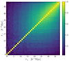 |
Fig. 3. Normalized covariance matrix for wp(r⊥), computed from the 1687 fiducial cosmology simulations in the ABACUSSMALL dataset. |
Sampling is performed using the EMCEE python package (Foreman-Mackey et al. 2013), employing the differential evolution algorithm (Braak 2006). The MCMC chain is assigned initial parameter values of 𝒞fid and 𝒢fid, where a small Gaussian perturbation of 𝒩(0, 10−3) is added to each parameter. Samples are drawn from a flat prior distribution of 𝒞 and 𝒢, with prior ranges given in Tables 1 and 2, respectively.
In addition to the inference analysis, we sampled the posterior distribution of the cosmological parameters with HOD parameters fixed to their fiducial value and vice versa, which helped us identify and address degeneracies between the two parameter sets. This analysis is vital to identify potential supplementary statistics to add to our model to better constrain HOD parameters. Such tailored analysis is unsuitable for real data due to underestimation and bias in error measurements, underscoring the mock dataset’s importance during model development.
6. Results
6.1. Emulator performance
The emulator’s prediction of ξR is shown in Fig. 4, with one random sample from every cosmology in the test dataset shown in the upper panel. In the bottom panel, we show relative errors of the individual samples from the upper panel and include the mean and median errors computed from the test dataset. The emulator accuracy increases as the extreme separation distances are approached, where Poisson noise becomes increasingly dominant. On intermediate scales, the emulator achieves sub-percent accuracy with relative errors below 1% for 1 ≲ r/(h−1 Mpc)≲30.
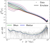 |
Fig. 4. Upper panel: Example set of ξR sampled from 29 cosmologies in the test and validation datasets, comparing data measurements with emulator predictions. We scale ξR with r to emphasize the accuracy on large scales. Lower panel: Relative error of the prediction samples from the upper panel (gray lines) and the mean and median relative error from all samples in the test data. |
Figure 5 shows the emulator prediction of wp in the upper panel, using the same test samples as in Fig. 4. The data points correspond to direct measurements of wp using the redshift space coordinates of galaxies. Relative errors from each sample are shown in the lower panel, including mean and median errors computed from all test simulations. Compared to the errors of ξR, the emulator predicts wp more accurately, with errors below 2% for r⊥ ≲ 20 h−1 Mpc. The projection results in an overall smoothing of the relative errors of wp compared to ξR, with reduced errors toward the extreme ends and increased errors on intermediate scales. This indicates that some information is lost during the projection of ξR.
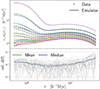 |
Fig. 5. Upper panel: Example set of wp sampled from 29 cosmologies in the test and validation datasets, with solid lines corresponding to the integrated samples of ξR in Fig. 4. Data points show direct measurements of wp in redshift space. Lower panel: Relative difference between wp from direct measurements and from integrating |

The largest emulator errors corresponded to specific HOD parameter combinations that produced noisy samples of ξR on large scales where ξR dropped by orders of magnitude from one measurement to the next. These outliers occurred after limiting the separation scales to r ≤ 105 h−1 Mpc. Combined with the prominent shot noise in ξR at r ≳ 60 h−1 Mpc, this suggests that the bin resolution was too narrow on large scales.
We note that the c002 simulation has the highest value of w0 of all cosmologies considered, and is thus outside the training range of the emulator. Nonetheless, relative error from this simulation was lower than the mean and median error from test simulations. Additionally, we did not ensure that the extreme values of the generated HOD parameters belonged to the training set, which caused some to be found in the testing and validation set.
6.2. Parameter inference
Figure 6 shows the posterior distributions of the cosmological parameters, marginalized over the HOD parameters. The posterior of baryonic density ωb is poorly constrained using the projected 2PCF data alone, and therefore not shown in the plot. This is also a consequence of using an overly simplistic HOD model and the absence of the information of baryonic acoustic oscillations. Several parameters have wide marginalized distributions, indicating that our model cannot put significant constraints on them from wp at z = 0.25 over the separation scale considered.
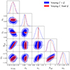 |
Fig. 6. Recovery test of the fiducial cosmology after marginalizing over the HOD parameters (in blue) and keeping the HOD parameters fixed (in red). |
The posterior distributions of ωcdm and σ8 suggest a tighter constraint on these parameters since the two parameters directly impact structure formation. There appears to be no considerable degeneracy between ωcdm and the HOD parameters. On the other hand, σ8 shows distinct levels of degeneracy with the HOD parameters since its effect on the 2PCF can easily be compensated by changes in HOD parameters. Similar results were obtained by Miyatake et al. (2022, Fig. 9), who were able to constrain Ωm and σ8 well using wp only using the DARKQUEST data.
We note that one of the equation of state parameters, wa, is poorly constrained by our model. This can be explained by the fact that our analysis is restricted to a single redshift, we cannot expect our model to appropriately account for dynamic dark energy. However, Cuesta-Lazaro et al. (2024, Fig. 6) obtains similar constraints for these parameters using ξS, but their constraints are significantly improved when including signals from density-split clustering, suggesting that the two parameters could be constrained with a single redshift only.
The HOD parameter posterior distributions are shown in Fig. 7. The HOD parameters that are well constrained are  and M1, which are the two parameters most strongly affecting the central and satellite galaxy distributions. Both parameters show some degeneracy with the cosmological parameters, most notably in the marginalized distributions of
  . This is expected, as cosmological parameters affect the resulting
  through the halo mass function. The parameters σlog M and α are relatively poorly constrained. Their posteriors, when varying HOD parameters only, suggest that wider prior ranges should be considered, as in Cuesta-Lazaro et al. (2024, Table 1). Our results are consistent with previous studies, such as Zentner et al. (2019, Fig. 1), in which HOD parameters are poorly constrained by wp alone.
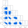 |
Fig. 7. Marginalized posterior of the HOD parameters. The true parameters in the recovery test are shown in black. |
To further validate our pipeline, we performed additional recovery tests using two different cosmologies. The results are presented in Fig. 8. We find that the true cosmological parameters are consistently recovered within 2σ for both cosmological models. This demonstrates the robustness of our method across different cosmologies and supports the reliability of our parameter constraining procedure.
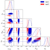 |
Fig. 8. Recovery tests for two different fiducial cosmologies selected from the test dataset. The true parameter values are indicated by the colored horizontal and vertical dashed lines. |
7. Discussion
Our analysis of parameter degeneracies is mainly limited to degeneracies between the cosmological and HOD parameters. To accurately discern the impact on a specific parameter, it is essential to consider the intrinsic constraining power that the parameter in question exerts on the observable. Our analysis of these degeneracies is hindered by the model’s limited ability to tightly constrain several parameters. As a result, further extensions to the model are necessary to adequately discriminate the effects of the two parameter sets. Moreover, degeneracies within each parameter set are not addressed in our current study.
A significant limitation of our recovery test is the primitive estimation of the covariance matrix. Most notably, emulator errors are not accounted for. As illustrated in Fig. 5, the predictions of our emulator are less accurate at extreme scales, which is a factor that is not incorporated into the likelihood model in Eq. (16). Furthermore, the errors among individual measurements of wp used to construct the mock data vector, as shown in Fig. 2, are neglected. Developing a more realistic covariance matrix is the essential first step toward applying this emulator-based approach to real data. Consequently, we are unable to draw definitive conclusions about the true constraining power of our model. After refining the current likelihood estimation of our model, a second clustering statistic should be added before further explorations of the information content of our inference analysis is considered, such as the scale dependence of parameter’s constraints.
Bias parameters are among the critical ingredients missing in the base model of Zheng et al. (2005). Both halo assembly bias, referring to halos of equal mass exhibiting different clustering properties, and galaxy assembly bias, referring to variations in the number of galaxies hosted by halos of identical mass, have been omitted in our analysis. Cuesta-Lazaro et al. (2023, Fig. 10), for instance, shows how including environmental-based assembly bias can induce a shift in the constraint of σ8 more than 1σ from their fiducial value. Other effects, such as velocity biases, are often introduced to allow a galaxy’s peculiar velocity to be slightly offset from that of its host halo, which is supported by observational evidence (Yuan et al. 2022). In future analyses, we plan to construct refined galaxy catalogs using the highly efficient PYTHON package ABACUSHOD (Yuan et al. 2022), which includes a large variety of modern HOD variations and is specifically designed to work with the ABACUSSUMMIT simulation suite.
Several works in the literature also emulate galaxy clustering statistics using different simulation suites, such as the AEMULUS project (Zhai et al. 2019, 2023; Storey-Fisher et al. 2024) and the Mira-Titan project (Kwan et al. 2023). These simulations cover a similar range of cosmological parameter space as the ABACUS simulations, but feature different extensions to the baseline Λ cold dark matter model, such as massive neutrinos and dynamical dark energy. In contrast to previous works, which typically use Gaussian process regression, we adopted fully connected neural networks for our emulator construction. Neural networks are particularly well suited for handling large datasets, unlike Gaussian process regression, which scales as 𝒪(N3), with N being the size of the training dataset.
8. Conclusions
Emulators provide an efficient method for bypassing the prohibitively expensive computational demands of running full N-body simulations to model galaxy clustering statistics on nonlinear scales. We have introduced a model designed to predict the real-space correlation function of galaxies over the range r ∈ [0.1, 105] h−1 Mpc. The key strength of this approach lies in its computational efficiency, which enables a near-instantaneous estimation of the correlation function given a set of cosmological parameters. This was achieved by constructing galaxy catalogs using a straightforward HOD model applied to halos from the ABACUSSUMMIT simulation suite.
Our emulator predicts the projected correlation function over a wide range of scales, with sub-percent accuracies on scales 1 ≲ r⊥/(h−1 Mpc)≲10. Using this model, we conducted inference analyses to constrain key cosmological parameters, particularly ωcdm and σ8. While these analyses demonstrate the model’s capability, the limited information provided by the projected correlation function alone prevents us from placing stronger constraints on other cosmological parameters. This issue can be addressed by incorporating the information from redshift-space clustering, which we plan to explore in future work. Furthermore, our analysis reveals that the simplified covariance matrix employed does not account for emulator errors, highlighting the need for further refinement of our methodology before drawing definitive conclusions. Despite these limitations, our results are consistent with previous studies regarding the constraining power of the projected correlation function.
Future work in developing an emulator-based model for large-scale structure analysis will focus on incorporating additional summary statistics to enhance the model’s ability to probe underlying cosmological information, such as higher-order clustering statistics, density-split clustering (Cuesta-Lazaro et al. 2024; Paillas et al. 2024), and the marked correlation function (Storey-Fisher et al. 2024). Additionally, by employing a more sophisticated HOD model, we aim to generate galaxy catalogs that more accurately reflect the complexities of galaxy clustering. At present, our model cannot robustly marginalize over the HOD parameters, a limitation we intend to address. Once this is achieved, we plan to apply our model to observational data from the ongoing Euclid survey to further refine cosmological parameter estimates.
Acknowledgments
We thank the Research Council of Norway for their support and the resources provided by UNINETT Sigma2 – the National Infrastructure for High-Performance Computing and Data Storage in Norway. We are grateful to the editor and the anonymous reviewer for their valuable comments and suggestions.
References
- Agarap, A. F. 2019, ArXiv e-prints [arXiv:1803.08375] [Google Scholar]
- Alam, S., Aubert, M., Avila, S., et al. 2021, Phys. Rev. D, 103, 083533 [NASA ADS] [CrossRef] [Google Scholar]
- Berlind, A. A., & Weinberg, D. H. 2002, ApJ, 575, 587 [Google Scholar]
- Braak, C. J. F. T. 2006, Stat. Comput., 16, 239 [NASA ADS] [CrossRef] [Google Scholar]
- Burger, P. A., Paillas, E., & Hudson, M. J. 2024, Phys. Rev. D, 110, 083517 [Google Scholar]
- Chevallier, M., & Polarski, D. 2001, Int. J. Mod. Phys. D, 10, 213 [Google Scholar]
- Cole, S., Percival, W. J., Peacock, J. A., et al. 2005, MNRAS, 362, 505 [Google Scholar]
- Colless, M., Dalton, G., Maddox, S., et al. 2001, MNRAS, 328, 1039 [Google Scholar]
- Cuesta-Lazaro, C., Nishimichi, T., Kobayashi, Y., et al. 2023, MNRAS, 523, 3219 [CrossRef] [Google Scholar]
- Cuesta-Lazaro, C., Paillas, E., Yuan, S., et al. 2024, MNRAS, 531, 3336 [Google Scholar]
- Dawson, K. S., Schlegel, D. J., Ahn, C. P., et al. 2013, AJ, 145, 10 [Google Scholar]
- Dawson, K. S., Kneib, J.-P., Percival, W. J., et al. 2016, AJ, 151, 44 [Google Scholar]
- DESI Collaboration (Aghamousa, A., et al.) 2016, ArXiv e-prints [arXiv:1611.00036] [Google Scholar]
- Diemer, B., & Joyce, M. 2019, ApJ, 871, 168 [NASA ADS] [CrossRef] [Google Scholar]
- Drinkwater, M. J., Jurek, R. J., Blake, C., et al. 2010, MNRAS, 401, 1429 [CrossRef] [Google Scholar]
- Foreman-Mackey, D., Hogg, D. W., Lang, D., & Goodman, J. 2013, PASP, 125, 306 [Google Scholar]
- Guo, H., Zheng, Z., Zehavi, I., et al. 2014, MNRAS, 441, 2398 [NASA ADS] [CrossRef] [Google Scholar]
- Guo, H., Zheng, Z., Zehavi, I., et al. 2015, MNRAS, 453, 4368 [Google Scholar]
- Hadzhiyska, B., Eisenstein, D., Bose, S., Garrison, L. H., & Maksimova, N. 2021, MNRAS, 509, 501 [NASA ADS] [CrossRef] [Google Scholar]
- Hendrycks, D., & Gimpel, K. 2016, ArXiv e-prints [arXiv:1606.08415] [Google Scholar]
- Kingma, D. P., & Ba, J. 2017, ArXiv e-prints [arXiv:1412.6980] [Google Scholar]
- Kobayashi, Y., Nishimichi, T., Takada, M., & Miyatake, H. 2022, Phys. Rev. D, 105, 083517 [CrossRef] [Google Scholar]
- Kwan, J., Heitmann, K., Habib, S., et al. 2015, ApJ, 810, 35 [CrossRef] [Google Scholar]
- Kwan, J., Saito, S., Leauthaud, A., et al. 2023, ApJ, 952, 80 [NASA ADS] [CrossRef] [Google Scholar]
- Laureijs, R., Amiaux, J., Arduini, S., et al. 2011, ArXiv e-prints [arXiv:1110.3193] [Google Scholar]
- Linder, E. V. 2003, Phys. Rev. Lett., 90, 091301 [Google Scholar]
- Majumdar, A., & Arora, R. 2019, CORRFUNC: Blazing Fast Correlation Functions with AVX512F SIMD Intrinsics (Singapore: Springer Singapore) [Google Scholar]
- Maksimova, N. A., Garrison, L. H., Eisenstein, D. J., et al. 2021, MNRAS, 508, 4017 [NASA ADS] [CrossRef] [Google Scholar]
- Miyatake, H., Kobayashi, Y., Takada, M., et al. 2022, Phys. Rev. D, 106, 083519 [NASA ADS] [CrossRef] [Google Scholar]
- Navarro, J. F., Frenk, C. S., & White, S. D. M. 1997, ApJ, 490, 493 [Google Scholar]
- Nishimichi, T., Takada, M., Takahashi, R., et al. 2019, ApJ, 884, 29 [NASA ADS] [CrossRef] [Google Scholar]
- Paillas, E., Cuesta-Lazaro, C., Percival, W. J., et al. 2024, MNRAS, 531, 898 [Google Scholar]
- Peacock, J. A., & Smith, R. E. 2000, MNRAS, 318, 1144 [Google Scholar]
- Planck Collaboration VI. 2020, A&A, 641, A6 [NASA ADS] [CrossRef] [EDP Sciences] [Google Scholar]
- Saves, P., Lafage, R., Bartoli, N., et al. 2024, Adv. Eng. Softw., 188, 103571 [Google Scholar]
- Seljak, U. 2000, MNRAS, 318, 203 [Google Scholar]
- Sinha, M., & Garrison, L. H. 2020, MNRAS, 491, 3022 [Google Scholar]
- Srivastava, N., Hinton, G., Krizhevsky, A., Sutskever, I., & Salakhutdinov, R. 2014, J. Mach. Learn. Res., 15, 1929 [Google Scholar]
- Storey-Fisher, K., Tinker, J. L., Zhai, Z., et al. 2024, ApJ, 961, 208 [NASA ADS] [CrossRef] [Google Scholar]
- York, D. G., Adelman, J., Anderson, J. E., et al. 2000, AJ, 120, 1579 [Google Scholar]
- Yuan, S., Garrison, L. H., Hadzhiyska, B., Bose, S., & Eisenstein, D. J. 2022, MNRAS, 510, 3301 [NASA ADS] [CrossRef] [Google Scholar]
- Zentner, A. R., Hearin, A., van den Bosch, F. C., Lange, J. U., & Villarreal, A. S. 2019, MNRAS, 485, 1196 [NASA ADS] [CrossRef] [Google Scholar]
- Zhai, Z., Tinker, J. L., Becker, M. R., et al. 2019, ApJ, 874, 95 [CrossRef] [Google Scholar]
- Zhai, Z., Tinker, J. L., Banerjee, A., et al. 2023, ApJ, 948, 99 [NASA ADS] [CrossRef] [Google Scholar]
- Zheng, Z., Berlind, A. A., Weinberg, D. H., et al. 2005, ApJ, 633, 791 [NASA ADS] [CrossRef] [Google Scholar]
- Zheng, Z., Zehavi, I., Eisenstein, D. J., Weinberg, D. H., & Jing, Y. P. 2009, ApJ, 707, 554 [Google Scholar]
All Tables
All Figures
|
Fig. 1. Cosmological parameters used in the training, testing, and validation datasets. Note that the fiducial parameter values are included in the test dataset. The large number of fiducial values for some parameters is due to the linear derivative varying two parameters at a time and the fixed parameter subsets of the broad emulator grid. |
| In the text | |
|
Fig. 2. Mock data vector wpdata(r⊥) (red) computed from averaging over the individual wp from the 25 fiducial cosmologies (blue). The error bars show the standard deviation of the individual wp samples. |
| In the text | |
|
Fig. 3. Normalized covariance matrix for wp(r⊥), computed from the 1687 fiducial cosmology simulations in the ABACUSSMALL dataset. |
| In the text | |
|
Fig. 4. Upper panel: Example set of ξR sampled from 29 cosmologies in the test and validation datasets, comparing data measurements with emulator predictions. We scale ξR with r to emphasize the accuracy on large scales. Lower panel: Relative error of the prediction samples from the upper panel (gray lines) and the mean and median relative error from all samples in the test data. |
| In the text | |
|
Fig. 5. Upper panel: Example set of wp sampled from 29 cosmologies in the test and validation datasets, with solid lines corresponding to the integrated samples of ξR in Fig. 4. Data points show direct measurements of wp in redshift space. Lower panel: Relative difference between wp from direct measurements and from integrating |
| In the text | |
|
Fig. 6. Recovery test of the fiducial cosmology after marginalizing over the HOD parameters (in blue) and keeping the HOD parameters fixed (in red). |
| In the text | |
|
Fig. 7. Marginalized posterior of the HOD parameters. The true parameters in the recovery test are shown in black. |
| In the text | |
|
Fig. 8. Recovery tests for two different fiducial cosmologies selected from the test dataset. The true parameter values are indicated by the colored horizontal and vertical dashed lines. |
| In the text | |
Current usage metrics show cumulative count of Article Views (full-text article views including HTML views, PDF and ePub downloads, according to the available data) and Abstracts Views on Vision4Press platform.
Data correspond to usage on the plateform after 2015. The current usage metrics is available 48-96 hours after online publication and is updated daily on week days.
Initial download of the metrics may take a while.