| Issue |
A&A
Volume 675, July 2023
|
|
|---|---|---|
| Article Number | A189 | |
| Number of page(s) | 25 | |
| Section | Cosmology (including clusters of galaxies) | |
| DOI | https://doi.org/10.1051/0004-6361/202245158 | |
| Published online | 20 July 2023 | |
KiDS-1000: Combined halo-model cosmology constraints from galaxy abundance, galaxy clustering, and galaxy-galaxy lensing
1
Ruhr University Bochum, Faculty of Physics and Astronomy, Astronomical Institute (AIRUB), German Centre for Cosmological Lensing, 44780 Bochum, Germany
e-mail: This email address is being protected from spambots. You need JavaScript enabled to view it.
2
Institute for Astronomy, University of Edinburgh, Royal Observatory, Blackford Hill, Edinburgh EH9 3HJ, UK
3
E. A. Milne Centre, University of Hull, Cottingham Road, Hull HU6 7RX, UK
4
Department of Physics and Astronomy, University College London, Gower Street, London WC1E 6BT, UK
5
Center for Theoretical Physics, Polish Academy of Sciences, al. Lotników 32/46, 02-668 Warsaw, Poland
6
Institute for Theoretical Physics, Utrecht University, 3584 CC Utrecht, The Netherlands
7
Leiden Observatory, Leiden University, PO Box 9513 2300 RA Leiden, The Netherlands
8
Department of Computer Science, University of British Columbia, 6224 Agricultural Road, Vancouver, BC V6T 1Z1, Canada
9
Kobayashi-Maskawa Institute for the Origin of Particles and the Universe (KMI), Nagoya University, Nagoya 464-8602, Japan
10
Institute for Advanced Research, Nagoya University, Nagoya 464-8601, Japan
11
Kavli Institute for the Physics and Mathematics of the Universe (WPI), The University of Tokyo Institutes for Advanced Study, The University of Tokyo, Chiba 277-8583, Japan
12
Center for Gravitational Physics and Quantum Information, Yukawa Institute for Theoretical Physics, Kyoto University, Kyoto 606-8502, Japan
13
Argelander-Institut für Astronomie, Universität Bonn, Auf dem Hügel 71, 53121 Bonn, Germany
Received:
6
October
2022
Accepted:
8
June
2023
Abstract
We present constraints on the flat Λ cold dark matter cosmological model through a joint analysis of galaxy abundance, galaxy clustering, and galaxy-galaxy lensing observables with the Kilo-Degree Survey. Our theoretical model combines a flexible conditional stellar mass function, which describes the galaxy-halo connection, with a cosmological N-body simulation-calibrated halo model, which describes the non-linear matter field. Our magnitude-limited bright galaxy sample combines nine-band optical-to-near-infrared photometry with an extensive and complete spectroscopic training sample to provide accurate redshift and stellar mass estimates. Our faint galaxy sample provides a background of accurately calibrated lensing measurements. We constrain the structure growth parameter to S8 = σ8√Ωm/0.3 =√0.773−0.030+0.028 and the matter density parameter to Ωm = 0.290−0.017+0.021. The galaxy-halo connection model adopted in the work is shown to be in agreement with previous studies. Our constraints on cosmological parameters are comparable to, and consistent with, joint ‘3 × 2pt’ clustering-lensing analyses that additionally include a cosmic shear observable. This analysis therefore brings attention to the significant constraining power in the often excluded non-linear scales for galaxy clustering and galaxy-galaxy lensing observables. By adopting a theoretical model that accounts for non-linear halo bias, halo exclusion, scale-dependent galaxy bias, and the impact of baryon feedback, this work demonstrates the potential for, and a way towards, including non-linear scales in cosmological analyses. Varying the width of the satellite galaxy distribution with an additional parameter yields a strong preference for sub-Poissonian variance, improving the goodness of fit by 0.18 in terms of the reduced χ2 value (and increasing the p-value by 0.25) compared to a fixed Poisson distribution.
Key words: gravitational lensing: weak / methods: statistical / cosmological parameters / galaxies: halos / dark matter / large-scale structure of Universe
© The Authors 2023
 Open Access article, published by EDP Sciences, under the terms of the Creative Commons Attribution License (https://creativecommons.org/licenses/by/4.0), which permits unrestricted use, distribution, and reproduction in any medium, provided the original work is properly cited.
This article is published in open access under the Subscribe to Open model. This email address is being protected from spambots. You need JavaScript enabled to view it. to support open access publication.
1. Introduction
In the last quarter of a century, we have seen the rise and establishment of the concordance cosmological model, which describes the formation and subsequent evolution of the cosmic structure. In this concordance model the Universe at the present time is modelled as a flat, cold dark matter (CDM) and cosmological constant (Λ) dominated Universe, with a negligible contribution from neutrinos, and gravity described by the law of General Relativity. Furthermore, the initial power spectrum of density fluctuations is assumed to be a single power law. Such ΛCDM models are described using only six free parameters, which govern the energy densities of baryons, Ωb, and the CDM, Ωdm; the spectral index, ns, and normalisation, σ8, of the density perturbations’ power spectrum; the Hubble parameter, H0; and the optical depth of re-ionisation. The flat geometry, implying that ΩΛ = 1 − Ωb − Ωdm, is strongly supported by high precision early-Universe measurements of the cosmic microwave background (CMB) temperature fluctuations combined with supernova and/or baryon acoustic oscillation distance measurements (Planck Collaboration VI 2020; Scolnic et al. 2018; Alam et al. 2021). Formally, the models also include the total neutrino mass, but the value of the parameter is too small for the current precision of observations (Gerbino & Lattanzi 2018).
A powerful probe of late-time cosmology is the large-scale distribution of galaxies. Even though stars contribute negligibly to the overall energy density of the Universe, the light from stars in galaxies can be used to trace the evolution of the underlying distribution of dark matter in two complementary ways. Firstly, the light path from distant galaxies is impacted by the distribution of foreground mass. This ‘gravitational lensing’ effect leads to a correlation between the observed shapes of galaxies, commonly referred to as cosmic shear. This observable can be used to probe the statistical properties of the total matter distribution in the Universe, typically quantified through the shape and amplitude of the matter power spectrum (Heymans et al. 2013; Hikage et al. 2019; Hamana et al. 2019; Asgari et al. 2021b; Secco et al. 2022; Amon et al. 2022a; van den Busch et al. 2022). Secondly, galaxies are expected to reside within dark matter haloes that form from the highest density peaks in the initial Gaussian random density field (e.g. Mo et al. 2010, and the references therein). Galaxies are therefore tracers of the underlying dark matter distribution, and with an accurate understanding of how biased these tracers are, the measurement of galaxy clustering as a function of redshift and scale places strong constraints on the properties of the ΛCDM model (see for example Alam et al. 2021). It is becoming increasingly common to combine these two different ‘two-point’ (2pt) statistics, along with a third measurement of the gravitational lensing of background galaxies by foreground galaxies, otherwise known as galaxy-galaxy lensing. These joint ‘3 × 2pt’ large-scale structure cosmological studies already have the precision to directly constrain some cosmological parameters independently of CMB measurements (Heymans et al. 2021; DES Collaboration 2022).
In this analysis we focus on exploiting the significant precision recovered with small-scale measurements of galaxy clustering and galaxy-galaxy lensing. These non-linear scales are typically excluded from cosmological analyses owing to insufficient or uncertain modelling of the complex relationship between galaxies and the underlying matter distribution on these scales (Davis et al. 1985; Dekel & Rees 1987). Galaxy bias is scale dependent, stochastic, and changes as a function of galaxy luminosity, colour, and morphological type (Dekel & Lahav 1999; Zehavi et al. 2011; Cacciato et al. 2012; Dvornik et al. 2018). Based on these facts, it is not surprising that galaxy bias is generally considered a nuisance to be marginalised over in the recovery of cosmological constraints. Many studies limit their analyses to scales where the galaxy bias is considered to be linear and scale independent (see for example van Uitert et al. 2018; Yoon et al. 2019; DES Collaboration 2022). An alternative approach uses perturbation theory (Desjacques et al. 2018) to expand galaxy bias modelling into the mildly non-linear regime (e.g. Mandelbaum et al. 2013; Sánchez et al. 2017; Heymans et al. 2021; Pandey et al. 2022). However, as a measurement of small-scale galaxy bias also contains a wealth of information regarding galaxy formation, we argue that it is preferential to utilise all the data, along with an appropriate galaxy bias model, to facilitate joint constraints on both cosmology and galaxy bias.
Given our previous attempts to shine a light on the galaxy bias and its properties (Dvornik et al. 2018), in this analysis we adopt a realistic and physically motivated halo model for galaxy bias. Under the assumption that all galaxies reside in dark matter haloes, we adopt a halo occupation distribution (HOD) model, a statistical description for how galaxies are distributed between and within the dark matter haloes (Peacock & Smith 2000; Scoccimarro et al. 2001; Mo et al. 2010; Yang et al. 2009; Cacciato et al. 2013, 2014; van den Bosch et al. 2013). When combined with the halo model, which describes the non-linear matter distribution as a sum of spherical dark matter haloes (Seljak 2000; Cooray & Sheth 2002), these models provide a fairly complete, broadly accurate1, and easy to understand description of galaxy bias, halo masses, and galaxy clustering (Cacciato et al. 2013).
Our approach builds on the cosmological analysis presented in Cacciato et al. (2013) and More et al. (2015), in which the halo model is used to coherently analyse the clustering of galaxies, the galaxy-galaxy lensing signal (Guzik & Seljak 2002; Yoo et al. 2006; Cacciato et al. 2009), and galaxy abundances as a function of luminosity or stellar mass (van den Bosch et al. 2013; Cacciato et al. 2013). Furthermore, the same approach was used to study the galaxy-halo connection exclusively, with a fixed cosmology, by Leauthaud et al. (2011) and Coupon et al. (2015). This combination of probes is hereafter referred to as ‘2 × 2 pt+SMF’, representing the combination of the two two-point statistics galaxy-galaxy lensing and galaxy clustering with the one-point stellar mass function (SMF). Analysis showing how much more information is in the 2 × 2 pt+SMF compared to the 2 × 2pt is nicely presented in More et al. (2013). The degeneracy breaking of model parameters arising from the inclusion of a SMF is shown in Mahony et al. (2022).
Since early applications, there has been significant interest in using the halo model to interpret large-scale structure probes (Seljak et al. 2005; Cacciato et al. 2009; Li et al. 2009). The analysis of 2 × 2pt statistics, down to non-linear scales, has been shown to lead to tight constraints for both Ωm and σ8 (Cacciato et al. 2013; Mandelbaum et al. 2013; More et al. 2015; Wibking et al. 2019). The halo model can also constrain extensions to the standard ΛCDM cosmologies, such as the equation of state of dark energy and neutrino mass (More et al. 2013; Krause & Eifler 2017). The choice of observables is motivated by the focus on a feasibility study on smaller scales that achieves similar precision, thus allowing for a direct and/or independent comparison to cosmic shear studies. In the era of high-precision cosmology, however, Miyatake et al. (2022a) show that the use of only a ‘broadly accurate’ standard halo model leads to significant offsets in the recovered cosmological parameters from a 2 × 2 pt analysis of HOD-populated numerical simulations. Consistency studies between the observed small-scale clustering and galaxy-galaxy lensing signals cast similar doubts on the accuracy of any standard halo model analysis (Leauthaud et al. 2017; Lange et al. 2021; Amon et al. 2022b).
Arguably the two most flawed approximations in the standard halo model formalism are (i) that haloes, and therefore galaxies, can overlap, and (ii) that haloes trace the matter distribution with a linear and scale-independent halo bias. Previous attempts to improve these approximations used halo exclusion formulations (Giocoli et al. 2010) to solve the first problem, combined with radial bias functions that add a scale dependence to the halo bias model (Tinker et al. 2005; van den Bosch et al. 2013; Cacciato et al. 2013).
In this analysis we instead follow the method proposed by Mead & Verde (2021), accounting for both scale-dependent non-linear halo bias and halo exclusion by incorporating the halo bias measured directly from the DARKEMULATOR suite of cosmological simulations (Nishimichi et al. 2019). As shown by Mahony et al. (2022), this necessary upgrade to the standard halo model leads to sufficient accuracy in the recovered cosmological parameters from a 2 × 2 pt+SMF analysis for the statistical power of current imaging surveys.
Other approximations in a halo model analysis include that the halo mass is the sole variable that determines the properties of the haloes and their occupying galaxies. Galaxy properties and the clustering of haloes are, however, expected to have a secondary dependence, on their local environment and assembly history (see Wechsler & Tinker 2018, and references therein). Furthermore, the adopted halo density profile is modelled from dark-matter-only numerical simulations, even though hydrodynamical simulations show that these profiles are modified by the presence of active galactic nuclei (Schaller et al. 2015; Wang et al. 2020). Debackere et al. (2021) show that, to account for baryon physics, it is sufficient to leave the concentration of dark matter haloes as a free parameter. Amon et al. (2022b) review the literature studies on the impact of these two approximations on 2 × 2 pt halo model studies with luminous red galaxies. Motivated by their conclusions, we chose to adopt nuisance parameters in our halo model to encapsulate the uncertainty of the impact of assembly bias and baryon feedback within our error budget.
In this paper we analyse the most recent data release from the Kilo-Degree Survey (KiDS), KiDS-1000 (Kuijken et al. 2019; Giblin et al. 2021; Hildebrandt et al. 2021), which spans over 1000 square degrees of imaging in nine bands from the optical through to the near-infrared. Our main ‘KiDS-Bright’ galaxy sample (Bilicki et al. 2021) benefits from the 180 square degree overlap between KiDS and the spectroscopic Galaxy And Mass Assembly (GAMA) survey (Driver et al. 2011). As an essentially complete spectroscopic survey to r < 19.8, GAMA serves as an extensive training set for machine learning and the calibration of different sample selections. The resulting GAMA-trained photometric redshifts and stellar mass estimates for the KiDS-Bright sample have an enhanced accuracy and precision that benefits this galaxy-galaxy lensing and galaxy clustering study. In order to simultaneously constrain cosmology and galaxy bias, we used the 2 × 2 pt+SMF combination of galaxy clustering and galaxy-galaxy lensing, as well as constraints on galaxy abundances in the form of the SMF.
We improve upon previous related 2 × 2 pt+SMF studies by (i) using a more accurate analytical model with the addition of non-linear halo bias (Mead & Verde 2021), taking the halo exclusion and scale dependence into account, (ii) taking the latest lensing and clustering data from a single survey, and (iii) using the full analytical covariance matrix, including the cross-variance between all observables. Our analysis is highly complementary to the emulator based 2 × 2 pt halo model analysis of the Hyper Suprime Camera (HSC) survey (Miyatake et al. 2022b).
Throughout this paper, all radii and densities are given in comoving units, ‘log’ is used to refer to the 10-based logarithm, and ‘ln’ for the natural logarithm. All the quantities that depend on the Hubble parameter adopt units of h, where h = H0/100 km s−1Mpc−1. We also use  as the present-day mean matter density of the Universe,
  , where
  and the halo masses are defined as
  enclosed by the radius rΔ, within which the mean density of the halo is Δ times
  , with Δ = 200.
This paper is organised as follows. In Sect. 2 we review our analytical model for computing the galaxy SMF, the galaxy-galaxy correlation function, and the galaxy-galaxy lensing signal using the halo model combined with a model that describes halo occupation statistics as a function of galaxy stellar mass. In Sect. 3 we introduce the 2 × 2 pt+SMF KiDS measurements, specifics of the covariance calculation, and our Bayesian analysis methodology. Our main results are presented in Sect. 4, and we conclude in Sect. 5.
2. The halo model
The halo model is an analytic framework that can be used to describe the clustering of matter and its evolution in the Universe (Seljak 2000; Peacock & Smith 2000; Cooray & Sheth 2002; van den Bosch et al. 2013; Mead et al. 2015). It is built upon the statistical description of the properties of dark matter haloes (namely the average density profile, large-scale bias, and abundance) as well as on the statistical description of the galaxies residing in them, using HOD. The model is sufficiently flexible to consistently describe the statistical weak lensing signal around a selection of galaxies, their clustering, abundances and cosmic shear signal.
2.1. Halo model ingredients
We assume that dark matter haloes are spherically symmetric on average, and have density profiles, ρ(r|M) = M uh(r|M), that depend only on their mass M, and uh(r|M) is the normalised density profile of a dark matter halo. Similarly, we assume that satellite galaxies in haloes of mass M follow a spherical number density distribution ns(r|M) = Ns us(r|M), where us(r|M) is the normalised density profile of satellite galaxies. All central galaxies are positioned at the centre of their halo: r = 0. We assume that the density profile of dark matter haloes follows a Navarro-Frenk-White (NFW) profile (Navarro et al. 1997). Since centrals and satellites are distributed differently, we write the galaxy-galaxy power spectrum, Pgg(k), as a combination of the central ‘c’, satellite ‘s’, and cross power spectrum, with
 (1)
(1)
and the galaxy-matter power spectrum, Pgm(k),
 (2)
(2)
Here  and
and  are the central and satellite fractions, respectively, and the average number densities
  ,
,  and
and  follow from
 (3)
(3)
where ‘x’ stands for ‘g’ (for galaxies), ‘c’ (for centrals), or ‘s’ (for satellites), ⟨Nx|M⟩ is the average number of galaxies given halo mass M, and n(M) is the halo mass function in the following form:
 (4)
(4)
with ν = δc/σ(M) being the peak height. Here δc is the critical overdensity required for spherical collapse at redshift z, and σ(M) is the mass variance. For f(ν) we used the fitting function to the numerical simulations presented in Tinker et al. (2010). In addition, it is common practice to split two-point statistics into a one-halo term (both points are located in the same halo) and a two-halo term (the two points are located in different haloes). The one-halo terms are
 (5)
(5)
 (6)
(6)
and all other terms are given by
 (7)
(7)
Here ‘x’ and ‘y’ are ‘c’ (central), ‘s’ (satellite), or ‘m’ (matter), 𝒫 is a Poisson parameter that captures the scatter in the number of satellite galaxies at fixed halo mass (in this case a free parameter – we define the 𝒫 in detail using Eqs. (24) and (25)), and we have defined the mass, central and satellite profiles as
 (8)
(8)
 (9)
(9)
and
 (10)
(10)
with  and
and  the Fourier transforms of the halo density profile and the satellite number density profile, respectively, both normalised to unity [
 ]. The various two-halo terms are given by
 (11)
(11)
where Plin(k) is the linear power spectrum, obtained using the Eisenstein & Hu (1998) matter transfer function, and bh(M, z) is the halo bias function. We adopted the Tinker et al. (2010) halo bias function, which, together with their halo mass function, provides a consistent normalisation of the halo model integrals. The second term in Eq. (11) encompasses the beyond-linear halo bias correction βNL proposed by Mead & Verde (2021), where
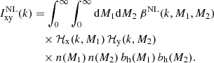 (12)
(12)
Here, βNL is measured using the DARKQUEST emulator (Nishimichi et al. 2019; Miyatake et al. 2022a; Mahony et al. 2022), by measuring the non-linear halo-halo power spectrum and then dividing it by the linear matter power spectrum multiplied with the product of linear bias factors (Mead & Verde 2021, Eq. (23)). Due to the definition of βNL, this measurement also holds true for galaxy-galaxy and galaxy-matter correlations. As shown in Mahony et al. (2022), this function is cosmology dependent, but does not account for assembly bias effects. In this paper, owing to the volume-limited mix of all types of galaxies used in our analysis, we consider any assembly bias to be a subdominant effect as the secondary properties are unlikely to manifest for a non-specific galaxy type selection (Wechsler & Tinker 2018). Numerically, the integrals in the halo model are not integrated from zero to infinity, but rather between a wide range of halo masses. Special care has to be taken to account for the masses outside of the integration limits, for which an appropriate correction is applied (as derived in Cacciato et al. 2009, Eqs. (24) and (25), and in Mead et al. 2020; Mead & Verde 2021, Appendices A in both papers). The two-point correlation functions corresponding to these power spectra are obtained via Fourier transformation:
 (13)
(13)
For the halo bias function, bh, we used the fitting function from Tinker et al. (2010), as it was obtained using the same numerical simulation from which the halo mass function was obtained. We have adopted the parametrisation of the concentration-mass relation given by Duffy et al. (2008):
![Mathematical equation: $$ \begin{aligned} c(M, z) = 10.14\; \ \left[\frac{M}{(2\times 10^{12} M_{\odot }/h)}\right]^{- 0.081}\ (1+z)^{-1.01}. \end{aligned} $$](/articles/aa/full_html/2023/07/aa45158-22/aa45158-22-eq29.gif) (14)
(14)
We allow for an additional normalisation, fh, s, such that
 (15)
(15)
where fh is the normalisation of the concentration-mass relation for dark matter haloes  , and fs is the normalisation of the concentration-mass relation for the distribution of satellite galaxies
  . The profiles
  and
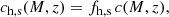
and  are both assumed to be non-truncated NFW profiles, with the same virial mass. Our adoption here of separate concentration-mass relations for dark matter haloes and satellite galaxies provides enough flexibility in the model to capture the uncertain impact of baryon feedback (for the scales adopted, Debackere et al. 2020, 2021; Amon et al. 2022b), and it has been used in the literature (Cacciato et al. 2013; Viola et al. 2015; van Uitert et al. 2016; Dvornik et al. 2018) to account for such effects. This additional flexibility is motivated by the fact that in the simulations, the active galactic nucleus (AGN) feedback pushes the baryons and dark matter from halo centres towards outskirts, and by that effectively changing the concentration of the matter distribution (Debackere et al. 2020; Mead et al. 2020). This is also supported by observations (Viola et al. 2015), which showed that the preferred value for the concentration normalisation is lower than 1. Using the halo model with these extra parameters is a benefit over the emulators that are based on dark-matter-only simulations (as for instance the DARKQUEST emulator Nishimichi et al. 2019; Miyatake et al. 2022a; Mahony et al. 2022), since they do not offer a simple way to accommodate for such flexibility, nor require simulations (Schneider & Teyssier 2015).
In the halo model we do not consider the mis-centred central term, as for a selection of galaxies the signature is accounted for through the terms for satellite galaxies, which do not reside in the centres of haloes by definition. What is more, the satellite galaxies populate haloes regardless of the existence of a central galaxy, which further removes the need for a mis-centred term (no central condition is enforced).
2.2. Conditional stellar mass function
We modelled the galaxy SMF and halo occupation statistics using the conditional stellar mass function (CSMF; motivated by Yang et al. 2008; Cacciato et al. 2009, 2013; Wang et al. 2013; van Uitert et al. 2016). The CSMF, Φ(M⋆|M), specifies the average number of galaxies of stellar mass, M⋆, that reside in a halo of mass, M. In this formalism, the halo occupation statistics of central galaxies are defined via the function
 (16)
(16)
In particular, the CSMF of central galaxies is modelled as a log-normal,
![Mathematical equation: $$ \begin{aligned} \Phi _{\mathrm{c} }(M_{\star } \vert M) = {1 \over {\sqrt{2\pi } \, {\ln }(10)\, \sigma _{\mathrm{c} } M_{\star } } }{\exp }\left[- { {\log (M_{\star } / M^{*}_{\mathrm{c} } )^2 } \over 2\,\sigma _{\mathrm{c} }^{2}} \right], \end{aligned} $$](/articles/aa/full_html/2023/07/aa45158-22/aa45158-22-eq36.gif) (17)
(17)
and the satellite term as a modified Schechter function,
![Mathematical equation: $$ \begin{aligned} \Phi _{\mathrm{s} }(M_{\star } \vert M) = { \phi ^{*}_{\mathrm{s} } \over M^{*}_{\mathrm{s} }}\, \left({M_{\star } \over M^{*}_{\mathrm{s} }}\right)^{\alpha _{\mathrm{s} }} \, {\exp } \left[- \left({M_{\star } \over M^{*}_{\mathrm{s} }}\right)^2 \right], \end{aligned} $$](/articles/aa/full_html/2023/07/aa45158-22/aa45158-22-eq37.gif) (18)
(18)
where σc is the scatter between stellar mass and halo mass and αs governs the power law behaviour of satellite galaxies. We note that  , σc,
, σc,  , αs, and
  are, in principle, all functions of the halo mass, M, but here we assume that σc and αs are independent of the halo mass, M. Inspired by Yang et al. (2008), who studied the halo occupation properties of galaxies in the Sloan Digital Sky Survey (SDSS), we parametrise
  ,
,  , and
, and  as
as
![Mathematical equation: $$ \begin{aligned} M^{*}_{\mathrm{c} }(M) = M_{0} \frac{(M/M_{1})^{\gamma _{1}}}{[1 + (M/M_{1})]^{\gamma _{1} - \gamma _{2}}}\,, \end{aligned} $$](/articles/aa/full_html/2023/07/aa45158-22/aa45158-22-eq44.gif) (19)
(19)
 (20)
(20)
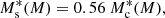
and
![Mathematical equation: $$ \begin{aligned} \log [\phi _{\mathrm{s} }^{*}(M)] = b_{0} + b_{1}(\log m_{13}), \end{aligned} $$](/articles/aa/full_html/2023/07/aa45158-22/aa45158-22-eq46.gif) (21)
(21)
where m13 = M/(1013 M⊙ h−1). In their analysis of the stellar-to-halo mass relation of GAMA galaxies, van Uitert et al. (2016) find that varying the pre-factor of 0.56 in Eq. (20) does not significantly affect the results; therefore, we retained this normalisation in our analysis. We can see that the stellar to halo mass relation for M ≪ M1 behaves as  and for M ≫ M1,
  , where M1 is a characteristic mass scale and M0 is a normalisation. Here γ1, γ2, b0 and b1 are all free parameters that govern the two slopes of the stellar-to-halo mass relation and the normalisation of the Schechter function. The choice of functional form of the CSMF is motivated by the good performance as seen in previous lensing and combined lensing and clustering studies. In Eq. (19), we adopt an effective stellar-to-halo mass relation for our mixed-population of red and blue galaxies. Bilicki et al. (2021) demonstrate a strong colour-dependence to this relationship, and future studies will investigate including a red/blue galaxy split in our analysis, which can also help improve the modelling of intrinsic galaxy alignments (e.g. Li et al. 2021).
From the CSMF it is straightforward to compute the galaxy SMF and the halo occupation numbers. The galaxy SMF is in this case given by
 (22)
(22)
and the average number of galaxies with stellar masses in the range M⋆, 1 ≤ M⋆ ≤ M⋆, 2 is given by
 (23)
(23)
where ‘x’ is ‘c’ (central), ‘s’ (satellite), or the total contribution from all galaxies. In order to predict the satellite-satellite term for the galaxy clustering power spectra (Eq. (6)), we used
 (24)
(24)
where 𝒫(M) is the mass-dependent Poisson parameter defined as
 (25)
(25)
which is unity if ⟨Ns|M⟩ is given by a Poisson distribution, larger than unity if the distribution is wider than a Poisson distribution (also called super-Poissonian distribution) or smaller than unity if the distribution is narrower than a Poisson distribution (also called sub-Poissonian distribution). In our fiducial analysis we limit ourselves to cases in which 𝒫(M) is independent of halo mass (𝒫(M) = 𝒫), and we treat 𝒫 as a free parameter. In Sect. 4.4 we present an extension to our fiducial analysis, allowing for mass dependence in the Poisson parameter, based on the observed distribution of satellite galaxies in the GAMA group catalogue (Robotham et al. 2011). Our findings are sensitive to the selection criteria chosen for the GAMA group catalogue. We are nevertheless able to conclude that assuming the Poisson parameter is independent of halo mass impacts our primary cosmological parameter constraints (mostly S8) at an acceptable ∼1σ level.
Overall, all the free parameters used to describe the HODs and the connection with the dark matter are
![Mathematical equation: $$ \begin{aligned} \lambda ^{\mathrm{HOD} } = [f_{\mathrm{h} }, M_0, M_1, \gamma _1, \gamma _2, \sigma _{\mathrm{c} }, f_{\mathrm{s} }, \alpha _{\mathrm{s} }, b_0, b_1, \mathcal{P} ]. \end{aligned} $$](/articles/aa/full_html/2023/07/aa45158-22/aa45158-22-eq53.gif) (26)
(26)
Priors on these parameters are broad, assuming wide uniform distributions, similar to the priors used in two studies of the galaxy-halo connection that both used GAMA and KiDS data (van Uitert et al. 2016; Dvornik et al. 2018). The HOD parameters could in principle also depend on redshift and halo mass, but furthering the complexity of the model, by increasing the number of parameters, would not be justified by the data. Our parameters describe an effective model over the redshift range in the analysis.
2.3. Projected lensing and clustering functions
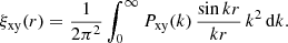
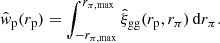
Once Pgg(k) and Pgm(k) have been determined, it is fairly straightforward to compute the projected galaxy-galaxy correlation function, wp(rp), and the excess surface density (ESD) profile, ΔΣ(rp). The projected galaxy-galaxy correlation function, wp(rp), is related to the real-space galaxy-galaxy correlation function, ξgg(r), according to
 (27)
(27)
Here ξgg(rp, rπ, z) is the redshift-space galaxy-galaxy correlation function, rπ is the redshift-space separation perpendicular to the line-of-sight and rπ, max is the maximum integration range used for the data (here we use rπ, max = 233h−1Mpc),  is the separation between the galaxies, ℒl(x) is the lth Legendre polynomial, and ξ0, ξ2, and ξ4 are given by
 (28)
(28)
![Mathematical equation: $$ \begin{aligned} \xi _2(r,z) = \left( {4 \over 3}\beta _{\mathrm{k} } + {4 \over 7}\beta _{\mathrm{k} }^2\right) \, \left[\xi _{\mathrm{gg} }(r,z) - 3 J_3(r,z)\right], \end{aligned} $$](/articles/aa/full_html/2023/07/aa45158-22/aa45158-22-eq57.gif) (29)
(29)
![Mathematical equation: $$ \begin{aligned} \xi _4(r,z) = {8 \over 35}\beta _{\mathrm{k} }^2 \, \left[\xi _{\mathrm{gg} }(r,z) + {15\over 2} J_3(r,z) - {35\over 2}J_5(r,z) \right], \end{aligned} $$](/articles/aa/full_html/2023/07/aa45158-22/aa45158-22-eq58.gif) (30)
(30)
where
 (31)
(31)
and
 (32)
(32)
with a = 1/(1 + z) the scale factor, D(z) the linear growth factor, and
 (33)
(33)
the mean bias of the galaxies in consideration. Equation (27) accounts for the large-scale redshift-space distortions due to infall (the ‘Kaiser’ effect), which is necessary because the measurements for wp(rp) are obtained for a finite rmax. We note that whilst this Kaiser (1987) formalism is only strictly valid in the linear regime, we adopt the non-linear galaxy-galaxy correlation function, ξgg(r), in Eqs. (28)–(30), with the non-linearities captured through the halo model power spectra in Eq. (13). van den Bosch et al. (2013) show that this modification provides a more accurate correction for the residual redshift space distortions, and that ignoring the presence of residual redshift space distortions leads to systematic errors that can easily exceed 20 percent on scales with rp > 10h−1 Mpc (Cacciato et al. 2013).
The ESD profile, ΔΣ(rp), is defined as
 (34)
(34)
Here Σ(rp) is the projected surface mass density, which is related to the galaxy-dark matter cross correlation, ξgm(r), according to
 (35)
(35)
The final model predictions and the covariance matrix are bin-averaged to the bin widths of the data vectors.
2.4. Cosmological parameters
The cosmological parameters in our model are described by the vector:
![Mathematical equation: $$ \begin{aligned} \lambda ^{\mathrm{cosmo} } = [\Omega _{\mathrm{m} }, \sigma _8, h, n_{\rm s}, \Omega _{\mathrm{b} }]. \end{aligned} $$](/articles/aa/full_html/2023/07/aa45158-22/aa45158-22-eq64.gif) (36)
(36)
As mentioned in Sect. 1, the goal of this paper is to use the ESD, wp and SMF data to constrain σ8 and Ωm. Because of that, we set the priors for those two parameters to be uninformative and set their ranges following the latest KiDS cosmic shear analysis (Asgari et al. 2021b). The last three cosmological parameters are shown to be poorly constrained using the ESD, wp, and SMF data (Cacciato et al. 2013; Mandelbaum et al. 2013); thus, they form a set of secondary cosmological parameters with informative priors. Priors and their ranges can be found in Table 22. In Appendix B we verify that our choice of priors do not inform the main cosmological parameters.
3. Data and sample selection
In this analysis we combine three observables from the KiDS: galaxy abundances in the form of the galaxy SMF, galaxy clustering in the form of the projected galaxy correlation function, and galaxy-galaxy lensing in the form of ESD profiles. Our KiDS observations were taken with OmegaCAM (Kuijken 2011), a 268-million pixel CCD mosaic camera mounted on the VLT Survey Telescope (VST). These instruments were designed to perform weak lensing measurements, with the camera and telescope combination providing a fairly uniform point spread function across the field-of-view (de Jong et al. 2013).
We analysed the latest data release of the KiDS survey (KiDS-1000, Kuijken et al. 2019), containing observations from 1006 square-degree survey tiles. Specifics of the survey, the calibration of the source shapes and photometric redshifts are described in Kuijken et al. (2019), Giblin et al. (2021), and Hildebrandt et al. (2021), respectively. The companion VISTA-VIKING (Edge et al. 2013) survey has provided complementary imaging in near-infrared bands (ZYJHKs), resulting in a unique deep, wide, nine-band imaging dataset (Wright et al. 2019). The default photo-z estimates provided as part of the KiDS survey were derived with the Bayesian photometric redshift (BPZ) approach (Benitez 2000).
We used shape measurements based on the r-band images, which have an average seeing of 0.66 arcsec. The galaxy shapes were measured using lensfit (Miller et al. 2013), which has been calibrated using image simulations described in Kannawadi et al. (2019). This provides galaxy ellipticities (ϵ1, ϵ2) with respect to an equatorial coordinate system, and an optimal weight.
The galaxies used for our lens and clustering sample were taken from the ‘KiDS-Bright’ sample (Bilicki et al. 2021). This sample mimics the selection of GAMA galaxies (Driver et al. 2011), by applying the condition mr < 20.0. For these galaxies a different method of determining the photometric redshifts was employed using the ANNz2 (artificial neural network) machine learning method (Sadeh et al. 2016), with the spectroscopic GAMA survey, which is 98.5% complete to r < 19.8, as a training set (Bilicki et al. 2018, 2021). Comparing the obtained redshifts with the spectroscopic redshifts from the matched galaxies between KiDS-Bright and GAMA, Bilicki et al. (2021) concluded that the ANNz2 photo-z are highly accurate with a mean offset of δz = 5 × 10⁻⁴, and a scaled mean absolute deviation scatter of σz = 0.018(1 + z).
Stellar mass estimates for the KiDS-Bright sample are obtained using the LEPHARE template fitting code (Arnouts et al. 1999; Ilbert et al. 2006). In these fits, ANNz2 photo-z estimates are used as input redshifts for each source, treating them as if they were exact, neglecting the percent error associated with the ANNz2 redshift. In practice, this error has little impact on the fidelity of the stellar mass estimates (Taylor et al. 2011). The estimates assume a Chabrier (2003) initial mass function, the Calzetti et al. (1994) dust-extinction law, Bruzual & Charlot (2003) stellar population synthesis models, and exponentially declining star formation histories. The input photometry to LEPHARE is extinction corrected using the Schlegel et al. (1998) maps with the Schlafly & Finkbeiner (2011) coefficients, as described in Kuijken et al. (2019).
Bilicki et al. (2021) found that the KiDS-Bright stellar mass estimates are in excellent agreement with independent stellar mass estimates from Wright et al. (2016) that combine GAMA spectroscopic redshifts with multi-wavelength imaging from 21 broadband filters from the far-UV to the far-IR. The median offset is  dex. Brouwer et al. (2021) estimated the overall systematic uncertainty on the stellar mass estimates of the KiDS-Bright sample, combining the uncertainty arising from the LEPHARE model fit, the photometric redshift scatter, and the difference found when exchanging elliptical aperture magnitudes for Sérsic model magnitudes. They estimated an overall uncertainty of σM* = 0.12 dex for the KiDS-Bright sample. This systematic uncertainty also includes the estimated Eddington systematic bias of ∼0.027 dex (Brouwer et al. 2021), which is estimated from the population of red and blue galaxies and it is considered a worst-case scenario. We chose to account for both statistical and systematic uncertainty in the stellar mass estimates through the nuisance parameter σc, in Eq. (17), which provides the freedom to model both the intrinsic and measurement noise scatter in the stellar-to-halo mass relation (Leauthaud et al. 2012; Bilicki et al. 2021). Furthermore, as the systematic and statistical uncertainties are comparable in power, the entries in the SMF and cross-covariances are inflated by a factor of 2 to account for the uncertainty arising from Eddington bias and the systematic shift in stellar masses, and not only through the σc parameter. Due to the weak cosmology dependence of the SMF, this primarily increases only the uncertainty of our HOD parameters, as the SMF is in the first place used to break degeneracies in our HOD part of the halo model.
3.1. Stellar mass function measurements and sample selection: SMF
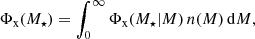
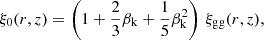
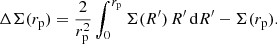
Our SMF measurements are performed using the maximum-volume weighting method (Schmidt 1968; Saunders et al. 1990; Cole 2011; Baldry et al. 2012; Wright et al. 2017). We weight each galaxy i by the inverse of the comoving volume over which the galaxy would be visible, given the magnitude limit of the whole sample, 1/Vmax, i. To estimate the number density Φ(M⋆), we have to derive M⋆, lim(z), the completeness in stellar mass as a function of redshift for our flux-limited sample. For the 1/Vmax technique, we need to know zmax, i, the maximum redshift beyond which galaxy i with stellar mass M⋆, i would no longer be part of the subsample (Weigel et al. 2016). This is done by determining the point at which the sample begins to become incomplete. Usually this process contains a potentially biased visual inspection. To avoid any bias, we instead adopt the automated method presented by Wright et al. (2017), using the MASSFUNCFITR package. The algorithm estimates the turnover point of the number density distribution in bins of comoving distance and stellar mass independently. In each fine bin of comoving distance, we take the mass at the peak density as the mass turnover point. In each fine bin of stellar mass, we take the largest comoving distance at median stellar mass density as the distance turnover point. The obtained turnover points are then fit with a high-degree polynomial resulting in a smooth form for the stellar mass limit as a function of redshift. This limit can be compared to the M* − zANNz2 distribution of the full KiDS-Bright galaxies in Fig. 1.
 |
Fig. 1. Galaxy stellar mass as a function of ANNz2 photometric redshift for the KiDS-Bright sample. The full sample is shown with a logarithmic hexagonal density plot. The blue line shows the stellar mass limit determined using the automated method presented by Wright et al. (2017). Red boxes show the six stellar mass bins used in the analysis, with individual galaxies plotted as black dots. The bin ranges were chosen in such a way as to achieve a good signal-to-noise ratio in all bins for our galaxy-galaxy lensing and galaxy clustering measurements. |
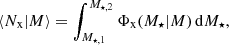
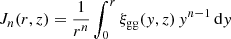
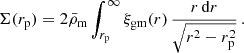
In Fig. 2 we present the SMF of the volume-limited KiDS-Bright sample from the galaxies in the 6 stellar mass bins, Φ(M⋆), which has a median redshift of z = 0.25. This is determined from the galaxy counts within the stellar mass limit, with errors derived analytically in Appendix A. We find good agreement between the KiDS measurement and the SMF from Wright et al. (2018), evaluated at the median redshift of our sample. Wright et al. (2018) is based on from an analysis using spectroscopic data from GAMA, Cosmic Evolution Survey (COSMOS), and the Hubble Space Telescope (HST). This comparison therefore demonstrates the agreement in the SMF between spectroscopic data and our photometric KiDS-Bright sample of galaxies, demonstrating that our stellar mass estimates are robust to the uncertainty in the photometric redshifts (Taylor et al. 2011; Bilicki et al. 2021; Brouwer et al. 2021).
 |
Fig. 2. KiDS-Bright galaxy SMF and the fractional errors. Upper panel: KiDS-Bright galaxy SMF (crosses) compared to the model from Wright et al. (2018), evaluated at the median redshift of our sample (black dashed line). The blue line and shaded region indicates the best-fit model and 68% confidence levels of our best-fit halo model (Eq. (22)). We caution that the quality of the fit cannot be judged by eye, because of the covariance in the data, between the data points and between the other observables. The reduced χ2 value for this observable is 1.05 (d.o.f. = 14.58, p-value = 0.39), estimated using the method presented in Appendix C. Lower panel: Fractional errors on the data and the model, ΔΦ/δΦ. |
As galaxy bias is inherently dependent on the stellar mass of the galaxy (Dvornik et al. 2018), we analyse the weak lensing and galaxy clustering of the KiDS-Bright galaxies grouped into 6 stellar mass bins. We chose to limit our analysis to galaxies within the stellar mass range of 9.1 < log(M⋆/h−2 M⊙)≤11.3, with the number of bins, and bin limits chosen in such a way as to achieve a similar and significant signal-to-noise ratio in all bins. Using the redshift-dependent stellar mass limit, we define upper redshift bounds to ensure each stellar mass bin is volume-limited, as indicated with red boxes in Fig. 1. The lower redshift bound is set to contain 95 percent of the volume-limited sample. The number of galaxies, median stellar mass and redshift of each bin is reported in Table 1.
KiDS-Bright stellar mass samples: overview of the number of lens galaxies, median stellar masses, M⋆, med, and median redshifts, zmed.
3.2. Galaxy-galaxy lensing measurement: ESD
As shown in Bilicki et al. (2021), the excellent ANNz2 photometric redshift estimates for the galaxies in the KiDS-Bright sample allow for robust estimates of their physical characteristics, in particular the stellar mass. In this section we combine this information with accurate shape measurements for more distant KiDS sources from Giblin et al. (2021) to measure the galaxy-galaxy lensing signal. To quantify the weak gravitational lensing signal, we used source galaxies from KiDS DR4 with a BPZ photo-z in the range 0.1 < zB < 1.2.
The lensing signal of an individual lens is too small to be detected, and hence we computed a weighted average of the tangential ellipticity ϵt as a function of projected distance rp using a large number of lens-source pairs. In the weak lensing regime this provides an unbiased estimate of the tangential shear, γt, which in turn can be related to the ESD, ΔΣ(rp), defined as the difference between the mean projected surface mass density inside a projected radius rp and the mean surface density at rp (as in Eq. (34); for more details, see Appendix C in Dvornik et al. 2018).
We computed a weighted average to account for the variation in the precision of the shear estimate, captured by the lensfit weight, ws (see Fenech Conti et al. 2017; Kannawadi et al. 2019, for details), and the fact that the amplitude of the lensing signal depends on the source redshift. The weight assigned to each lens-source pair is
 (37)
(37)
the product of the lensfit weight, ws, and the square of  – the effective inverse critical surface mass density, which is a geometric term that down-weights lens-source pairs that are close in redshift (e.g. Bartelmann & Schneider 2001).
We computed the effective inverse critical surface mass density for each lens using the photo-z of the lens zl and the full normalised redshift probability density of the sources, n(zs). The latter is calculated employing the self-organising map calibration method (Wright et al. 2020) as applied to KiDS DR4 in Hildebrandt et al. (2021). The resulting effective inverse critical surface density can be written as
 (38)
(38)
where D(zl), D(zs), and D(zl, zs) are the angular diameter distances to the lens, to the source, and between the lens and the source, respectively. For the lens redshifts, zl, we used the ANNz2 photo-z of the KiDS-Bright foreground galaxy sample. We implement the contribution of zl by integrating over the redshift probability distributions p(zl) of each lens. The lensing kernel is wide and therefore the resulting ESD signals are not sensitive to the small wings of the lens redshift probability distributions. We can thus safely approximate p(zl) as a normal distribution centred at the lenses photo-z, with a standard deviation σz/(1 + zl) = 0.018 (Bilicki et al. 2021). From previous KiDS galaxy-galaxy lensing studies we know that the error on the mean and width of source n(zs) are not biasing the galaxy-galaxy lensing signal (as shown in Dvornik et al. 2017).
For the source redshifts zs we follow the method used in Dvornik et al. (2018), by integrating over the part of the redshift probability distribution n(zs) where zs > zl. The galaxy source sample is specific to each lens redshift zl, with a minimum photometric redshift zs = zl + δz, with δz = 0.2 that is used to remove sources that are physically associated with the lenses. Thus, the ESD can be directly computed in bins of projected distance rp to the lenses as
![Mathematical equation: $$ \begin{aligned} \Delta \Sigma _{\mathrm{gm}} (r_{\mathrm{p} }) = \left[ \frac{\sum _{\mathrm{ls} }\widetilde{w}_{\mathrm{ls} }\epsilon _{\mathrm{t, s} }\Sigma _{\mathrm{cr, ls} }^{\prime }}{\sum _{\mathrm{ls} }\widetilde{w}_{\mathrm{ls} }} \right] \frac{1}{1+\overline{m}} \, , \end{aligned} $$](/articles/aa/full_html/2023/07/aa45158-22/aa45158-22-eq69.gif) (39)
(39)
where  , the sum is over all source-lens pairs in the distance bin, and
 (40)
(40)
is an average correction to the ESD profile that has to be applied to account for the multiplicative bias m in the lensfit shear estimates. The sum goes over thin redshift slices for which mi is obtained using image simulations (Kannawadi et al. 2019), weighted by w′ = ws D(zl,zs)/D(zs) for a given lens-source sample. The value of  is −0.003 for the six stellar mass bins, independent of the scale at which it is computed. The uncertainty in m is not marginalised over, as the contribution of the central m value is at most a percent of the total error budget of the galaxy-galaxy lensing signal.
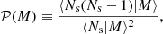
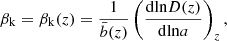
We note that the measurements presented here are not corrected for the contamination of the source sample by galaxies that are physically associated with the lenses (the so-called boost correction). The impact on ΔΣ is minimal, because of the weighting with the inverse square of the critical surface density in Eq. (38), (see for instance the bottom panel of Fig. A.4 in Dvornik et al. 2017) and the removal of the sources physically associated with the lens from our signal measurements. The effect of using photometric lenses in the ESD measurements is directly accounted for in our estimator and the covariance matrix. We subtract the signal around random points, which suppresses any large-scale systematics and sample variance (Singh et al. 2017). This empirical ‘random’ correction for large-scale sample variance has been shown to improve robustness on the measurement scales that are particularly relevant for constraining linear bias (Dvornik et al. 2018). We find the random correction for the KiDS-Bright sample becomes significant at scales R ≳ 3h−1 Mpc, rising to more than 100% of the ESD signal in the three lowest stellar mass bins, and it thus dictates the range of measurement scales we use in the analysis. On these large scales the random correction is more than four times larger than the statistical uncertainty (see Appendix D for details). The resulting random-corrected galaxy-galaxy lensing ESD measurements for the six stellar mass bins are shown in Fig. 3.
 |
Fig. 3. Galaxy-galaxy lensing: the stacked ESD profiles of the six stellar mass bins in the KiDS-Bright galaxy sample defined in Table 1. The solid lines represent the best fitting fiducial ESD halo model (Sect. 2.3, Eq. (34)) as obtained using an MCMC fit, with the 68 percent confidence interval indicated with a shaded region. We caution that the quality of the fit cannot be judged by eye, because of the covariance in the data between the observed bins and also between the observables. The reduced χ2 value for this observable is 1.28 (d.o.f. = 73.18, p-value = 0.05), estimated using the method presented in Appendix C. |
3.3. Projected galaxy clustering measurements: wp
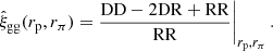
We measured the clustering of the KiDS-Bright galaxy sample using the Landy-Szalay (Landy & Szalay 1993) estimator for the galaxy correlation function:
 (41)
(41)
Here we count the number of galaxy-galaxy (DD), random-random (RR), and galaxy-random (DR) pairs, as a function of the pair’s transverse rp and radial rπ comoving separation. The accuracy of galaxy clustering measurements with this estimator depends critically on the quality of the random, R, catalogues. We used the Johnston et al. (2021a) organised random methodology that has been shown to recover unbiased clustering measurements in a series of mock galaxy catalogue analyses for the KiDS-Bright sample. Using machine learning, we infer the high-dimensional mapping between the observed on-sky galaxy number density and three systematic-tracer variables; atmospheric seeing, point spread function ellipticity and limiting magnitude. Systematically induced density variations across the survey footprint can then be defined. We randomly distribute clones of the real galaxies across the survey footprint, preserving the on-sky systematic density patterns, and matching the on-sky systematic-tracer properties to that of the clone’s parent galaxy. By retaining the photometric properties of the parent for each clone, selection effects are accurately mirrored in the organised randoms for any galaxy sub-sample, for example the 6 different stellar mass bins in our analysis. We used 20 times more randoms than data points, as presented by Johnston et al. (2021a).
The projected clustering correlation function is estimated through an integral over the line-of-sight separation, limited by a maximum defined distance, rπ, max,
 (42)
(42)
When analysing spectroscopic data, this continuous integral is estimated using a discrete sum, typically adopting uniform bins in rπ, with rπ, max ranging from 40 h−1 Mpc to 100 h−1 Mpc (as in for instance Mandelbaum et al. 2010; Farrow et al. 2015). Here the rπ, max limits are chosen to maximise the number of correlated galaxy pairs along the line-of-sight in the presence of redshift space distortions, whilst minimising the noise arising from the inclusion of uncorrelated objects. With our KiDS-Bright photometric sample we have an additional uncertainty in the true redshift, σz = 0.018(1 + z), which translates into an uncertainty on the radial distance of the order ∼100 h−1 Mpc, This renders the approach taken for spectroscopic samples sub-optimal in terms of signal-to-noise. We therefore chose to follow the approach of Johnston et al. (2021b) who optimised the projected galaxy clustering analysis of the photometric Physics of the Accelerating Universe Survey (PAUS), using dynamic binning in rπ out to a maximum rπ = 233 h−1 Mpc. This is motivated by the fact that PAUS photometric redshifts show a similar uncertainty as the KiDS-Bright sample. Using a mock galaxy catalogue, Johnston et al. (2021b) demonstrated that by allowing for an increase in the bin size from small to large values of rπ, their approach maximises the count of physically associated objects, whilst minimising noise at large-rπ with the broader bin size. Given the similar photometric redshift properties of KiDS-Bright and PAUS, we adopted their 12-rπ-bin adapted Fibonacci sequence in our estimator.
Johnston et al. (2021b) analysed mock GAMA galaxy catalogues with PAUS-like photometric redshifts to compare the projected clustering correlation function estimator  with the measurements using spectroscopic redshifts. Adopting dynamic binning and random galaxy catalogues that mimic both the position and photometric redshift uncertainty of the real galaxy sample, they found a roughly scale-independent bias with
  . As such, the dynamic binning and organised randoms only partially correct the correlation functions for the dilution introduced by photometric redshift uncertainty. Future work will focus on accounting for this dilution effect accurately in the theoretical prediction. For the purposes of this analysis, however, we chose to include a free dilution parameter 𝒟, which is used to correct the galaxy clustering measurements in the following way:
![Mathematical equation: $$ \begin{aligned} \hat{w}_{\mathrm{p, corr} }(r_{\mathrm{p} }) = [1+\mathcal{D} ]\, \hat{w}_{\mathrm{p} }(r_{\mathrm{p} }). \end{aligned} $$](/articles/aa/full_html/2023/07/aa45158-22/aa45158-22-eq77.gif) (43)
(43)
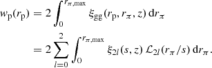
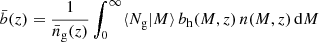
We adopted a uniform prior for 𝒟 with the range between 0 and 0.3 and used a single parameter to scale all six stellar mass bins. This prior was motivated by a series of mock KiDS-Bright galaxy clustering analysis using MICE2 (Fosalba et al. 2015a,b; Crocce et al. 2015; Carretero et al. 2015; Hoffmann et al. 2015), where we confirmed the findings of Johnston et al. (2021b) and found no strong dependence of the dilution effect on stellar mass. We note that a similar correction was applied to the Dark Energy Survey (DES) photometric clustering measurements (Pandey et al. 2022; DES Collaboration 2022, referred therein as Xlens). The prior and motivation behind the introduction of their systematic nuisance parameter differs, however. The resulting projected clustering measurements for the six stellar mass bins are shown in Fig. 4.
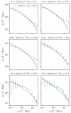 |
Fig. 4. Galaxy clustering: the projected galaxy clustering signal of the six stellar mass bins in the KiDS-Bright galaxy sample defined in Table 1. The solid lines represent the best fitting fiducial halo model (Sect. 2.3, Eq. (27)) as obtained using an MCMC fit, with the 68 percent confidence interval indicated with a shaded region. We caution that the quality of the fit cannot be judged by eye, because of the covariance in the data, between the observed bins and between the observables. The reduced χ2 value for this observable is 1.42 (d.o.f. = 71.62, p-value = 0.01), estimated using the method presented in Appendix C. |
3.4. Accounting for the cosmology dependence of distance measures
To obtain estimates of the SMF (Sect. 3.1, Fig. 2), the galaxy-galaxy lensing (ESD; Sect. 3.2, Fig. 3), and the projected galaxy clustering (wp, Sect. 3.3, Fig. 4), we adopted a fiducial flat ΛCDM cosmology with Ωm = 0.3 to compute distances. As such, our 2 × 2 pt+SMF data vector is cosmology dependent, with changes in the fiducial cosmology changing the distance-redshift relation, which in turn shifts galaxies between the stellar mass bins and lens-source pairs between the radial separation bins.
At the mean redshift of the KiDS-Bright sample, the effect of changing Ωm within our prior limits introduces changes in distance estimates at the level of a few percent. The approximation that the measurements are effectively independent of cosmological parameters within their observational uncertainties (Mandelbaum et al. 2013; Cacciato et al. 2013) no longer holds for surveys with a statistical power that is similar or better than KiDS.
In this analysis we account for the cosmology dependence of our data vector following the correction procedure presented in More (2013) and More et al. (2015), which modifies the model prediction for each cosmology targeted by the likelihood sampler. First we defined a cosmology-dependent comoving separation  for our target model, relative to the comoving separation, rp, that was used to calculate our data vectors at a fixed fiducial cosmological model,
![Mathematical equation: $$ \begin{aligned} r_{\mathrm{p} }^{\mathrm{model} } = r_{\mathrm{p} }^{\mathrm{fid} } \left[ \frac{\chi (z_{\mathrm{med} }, \mathcal{C} ^{\mathrm{model} })}{\chi (z_{\mathrm{med} }, \mathcal{C} ^{\mathrm{fid} })} \right]. \end{aligned} $$](/articles/aa/full_html/2023/07/aa45158-22/aa45158-22-eq79.gif) (44)
(44)
Here χ is the comoving distance to the median lens redshift zmed in our target cosmological model 𝒞model, or in our fiducial cosmological model 𝒞fid. The galaxy clustering prediction for our target model is then given by
![Mathematical equation: $$ \begin{aligned} \widetilde{w}_{\mathrm{p} }(r_{\mathrm{p} }) = { w}_{\mathrm{p} }(r_{\mathrm{p} }^{\mathrm{model} }) \left[ \frac{E^{\mathrm{model} }(z_{\mathrm{med} })}{E^{\mathrm{fid} }(z_{\mathrm{med} })} \right], \end{aligned} $$](/articles/aa/full_html/2023/07/aa45158-22/aa45158-22-eq80.gif) (45)
(45)
where E(z) is the Hubble parameter. The galaxy-galaxy lensing prediction for our target model is given by
![Mathematical equation: $$ \begin{aligned} \widetilde{\Delta \Sigma }(r_{\mathrm{p} }) = \Delta \Sigma (r_{\mathrm{p} }^{\mathrm{model} }) \left[ \frac{\Sigma _{\mathrm{cr} }^{\mathrm{model} }(z_{\mathrm{med} }, z_{\mathrm{s} })}{\Sigma _{\mathrm{cr} }^{\mathrm{fid} }(z_{\mathrm{med} }, z_{\mathrm{s} })} \right], \end{aligned} $$](/articles/aa/full_html/2023/07/aa45158-22/aa45158-22-eq81.gif) (46)
(46)
where Σcr is the critical surface density calculated for the median redshift of the lenses zmed and a fixed source redshift zs = 0.6. We note that calculating the more precise estimate for Σcr using Eq. (38) is not necessary in this instance, as Σcr only has a weak cosmology dependence. Finally, the predictions of abundances of galaxies in the target cosmology is given by
![Mathematical equation: $$ \begin{aligned} \widetilde{n}_{\mathrm{g} } = \overline{n}_{\mathrm{g} }^{\mathrm{model} } \left[ \frac{\chi ^{3}(z_{\mathrm{u} }, \mathcal{C} ^{\mathrm{model} }) - \chi ^{3}(z_{\mathrm{l} }, \mathcal{C} ^{\mathrm{model} })}{\chi ^{3}(z_{\mathrm{u} }, \mathcal{C} ^{\mathrm{fid} }) - \chi ^{3}(z_{\mathrm{l} }, \mathcal{C} ^{\mathrm{fid} })} \right], \end{aligned} $$](/articles/aa/full_html/2023/07/aa45158-22/aa45158-22-eq82.gif) (47)
(47)
which is implicitly correcting the surveyed volume in the SMF calculation. Here the zl and zu are the lower and upper redshift limits in our samples.
3.5. Covariance matrix
The covariance matrix used in this analysis is based on the analytical approach detailed in Dvornik et al. (2018) and Joachimi et al. (2021), with the addition of the analytical covariance matrix for the SMF and the cross terms between the SMF and two-point correlation functions. The new terms for the SMF covariance and the cross covariance between the SMF and two-point functions are presented in Appendix A. Our implementation of the analytical covariance derivation was validated against theory (Pielorz et al. 2010; Takada & Hu 2013; Li et al. 2014; Marian et al. 2015; Krause & Eifler 2017), independent software by Joachimi et al. (2021) and simulations (MICE2 Fosalba et al. 2015a,b; Carretero et al. 2015; Crocce et al. 2015; Hoffmann et al. 2015), following the validation approach of Blake et al. (2020) and Joachimi et al. (2021). Survey area effects on the variance were calculated using the accurate, survey-dependent and data-based HEALPIX method presented in Joachimi et al. (2021, Eq. (E.10)).
3.6. Likelihood and iterative updates
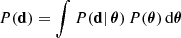
We used Bayesian inference to determine the posterior probability distribution P(θ | d) of the model parameters θ, given the data d. According to Bayes’ theorem, P(θ | d) is
 (48)
(48)
where P(d | θ) is the likelihood of the data given the model parameters, P(θ) is the prior probability of these parameters, and
 (49)
(49)
is the evidence for the model. Since we do not perform model selection in this analysis, the evidence just acts as a normalisation constant that we do not need to calculate. Given this, the likelihood distribution P(d | θ) is assumed to be Gaussian:
![Mathematical equation: $$ \begin{aligned} P(\mathbf d \, \vert \, \boldsymbol{\theta }) = \frac{1}{\sqrt{(2\pi )^{n}\vert \mathbf C \vert }} \exp \left[- \frac{1}{2}\left[\left(\mathbf m (\boldsymbol{\theta }) - \mathbf d \right)^{T}\mathbf{C }^{-1} \left(\mathbf m (\boldsymbol{\theta }) - \mathbf d \right) \right] \right], \end{aligned} $$](/articles/aa/full_html/2023/07/aa45158-22/aa45158-22-eq85.gif) (50)
(50)
where C is the full covariance matrix for all the observables, containing their auto- and cross-correlations, |C| its determinant, m(θ) the model given the parameters θ, and n the number of observable bins. Priors can be found in Table 2. For the Bayesian inference, we used the Markov chain Monte Carlo (MCMC) sampler EMCEE (Foreman-Mackey et al. 2013).
Marginal constraints on all model parameters, listed together with their priors.
The posterior distribution in such highly multi-dimensional parameter spaces has numerous degeneracies and can be very difficult to sample from. Thus, the choice of proposal distributions is very important in order to achieve fast convergence and reasonable acceptance fractions for the proposed walker positions. To do so, we combine the default stretch move in the emcee with the proposal function based on the kernel density estimator of the complementary ensemble of walkers (Foreman-Mackey et al. 2013)3 in such a way that at every step of the sampler run, there is a 50% chance of using one of the proposal methods. This setup has one downside, and that is that it uses many walkers, and thus computing power. On the other hand, the convergence is faster and the resulting auto-correlation times are shorter, giving us shorter MCMC chains overall.
During the MCMC runs we iteratively update the βNL measurement (as it is cosmology dependent), as running the emulator at each step of the chain is computationally not feasible. Thus, the βNL measurement is evaluated using the median of the current position of the walkers in the parameter space. This returns an effective value for the non-linear halo bias correction that is, over the run of the MCMC, representative of the median of corrections that would be applied to every single model iteration in the chain. In our pipeline, the number of steps between iterations can be set by the user and we find that updating the βNL values every 20 steps allows for a reasonable run time while providing enough updates to the βNL correction. On the other hand, the covariance matrix is only re-evaluated with the new parameters at the end of the MCMC run and checked. We find that the updated covariance matrix and halo model parameters do not affect the results of our fit as our initial cosmological and HOD parameters were set to the ones from Heymans et al. (2021) and van Uitert et al. (2016), and our final results are close to theirs. The covariance matrix is dominated by the shot and/or shape noise on the majority of scales.
To report our result, we used two methods to estimate our constraints and parameter values. One method uses the maximum statistics of the marginal posterior distributions for each parameter (MMAX). Here the asymmetric errors are estimated around the maximum point in iso-distribution levels to cover 68% of the marginal distribution. For the second method, we used the full posterior distribution to find the best fitting parameters – the maximum a posteriori (MAP) point – and used the methodology presented in Joachimi et al. (2021) to associate an error with this measurement with the projected highest posterior density (PJ-HPD) approach. While the former method produces more stable parameter errors, especially when the likelihood surface is sparsely sampled, its point estimates, in general, do not correspond to the best fitting parameter values. In contrast, the latter method will in general produce noisier error estimates with unbiased parameter values.
4. Results
Now we turn the focus to our results, presenting cosmological parameter constraints in Sect. 4.1, large-scale analysis in Sect. 4.2, constraints on the galaxy-halo connection in Sect. 4.3, and effect of modelling of satellite galaxies in Sect. 4.4. Further details are presented in Appendix E. To recap, our theoretical 2 × 2 pt+SMF model consists of 17 free parameters, two of which are our main cosmology parameters, with 3 more secondary cosmology parameters that are harder to constrain given the combination of observables, and 11 parameters describing the galaxy-halo connection in the form of the CSMF. With six stellar mass bins, and three observables, our combined data vector consists of 156 data points. In Appendix C we use mock data realisations to estimate the effective number of degrees of freedom for our analysis finding νeff = 147.55. Following the likelihood analysis described in Sect. 3.6 we are able to constrain 12 parameters, listed in Table 2 along with their prior ranges. We find the MAP provides a good fit4 to the data, with a reduced χ2 value of 1.07 and p(χ2|νeff) = 0.27.
We compare the prediction from our fiducial model, and its 68% confidence regions, to the measured galaxy abundance SMF in Fig. 2, the galaxy-galaxy lensing ESD in Fig. 3, and the galaxy clustering wp in Fig. 4, for all of the six stellar mass bins. We find that the model reproduces the overall trends in the data, such as the presence of the bump at ∼1 h−1 Mpc in ESD due to satellite galaxies, and the fact that the stronger signal is present where galaxies have higher stellar mass, showing that massive galaxies reside in more massive haloes. We note that some caution is needed when interpreting the results, as the quality of the fit cannot be judged by eye due to highly correlated data points. We find acceptable fits to each component of our 2 × 2 pt+SMF data vector (for details, see Appendix C). We note that the poorest fit is found for the wp section of our joint data vector with ![Mathematical equation: $ p[\chi^2(\mathit{w}_{\mathrm{p}}) | \nu_{\mathrm{eff}}^{\mathit{w}_{\mathrm{p}}}] = 0.01 $](/articles/aa/full_html/2023/07/aa45158-22/aa45158-22-eq110.gif) . Whilst a formally acceptable fit, this may indicate that our model is lacking the ability to correctly describe the photometric redshift dilution effect discussed in Sect. 3.3.
. Whilst a formally acceptable fit, this may indicate that our model is lacking the ability to correctly describe the photometric redshift dilution effect discussed in Sect. 3.3.
4.1. Cosmology constraints
We find the following cosmological parameter constraints from our simultaneous 2 × 2 pt+SMF analysis of the ESD, wp and SMF signals of galaxies in the KiDS-Bright sample,
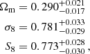
where 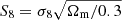 , and we quote the maximum statistics of the marginal posterior distributions (MMAX). The remaining cosmological parameters are unconstrained by our analysis, and informed by our choice of prior (see Fig. E.2). In Fig. 5 we present the 68% and 95% confidence levels of the joint two-dimensional, marginalised posterior distribution in the S8 − Ωm plane. The 2 × 2 pt+SMF constraints are shown to be in good agreement with constraints from KiDS cosmic shear and KiDS with BOSS 3 × 2pt constraints (Asgari et al. 2021b; Heymans et al. 2021). They are formally consistent, but in some mild tension with the Planck Collaboration VI (2020) TT,TE,EE+lowE CMB results. Using the Hellinger distance as a tension measure (see Heymans et al. 2021), the mild tension between our fiducial results and Planck is 1.9σ in S8.
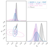 |
Fig. 5. Marginalised constraints for the joint distributions of S8 and Ωm. The 68% and 95% credible regions for the 2 × 2 pt+SMF fiducial analysis (blue) can be compared with constraints from KiDS cosmic shear (Asgari et al. 2021b, pink), KiDS with BOSS 3 × 2 pt (Heymans et al. 2021, purple), and the CMB Planck Collaboration VI (2020, black). |
In Fig. 6 we compare our constraints to a broader range of joint-probe large-scale structure analyses, finding consistency with all. Cacciato et al. (2013) and More et al. (2015) adopt a similar methodology, using a halo model formalism to jointly analyse galaxy-galaxy lensing, galaxy clustering, and galaxy abundance observables. Cacciato et al. (2013) analysed the seventh data release (DR7) of the SDSS. More et al. (2015) combined data from the Baryon Oscillation Spectroscopic Survey (BOSS) and the Canada France Hawaii Telescope Lensing Survey (CFHTLenS). The improved constraining power in this KiDS analysis reflects the significant increase in depth for the lensing sample relative to SDSS-DR7, and the ten-fold increase in area relative to CFHTLenS. We can also compare to 2 × 2 pt analyses that combine galaxy-galaxy lensing and galaxy clustering that introduce conservative scale cuts to reflect known limitations their adopted galaxy bias models. These include the fiducial analyses from DES, which adopt a linear galaxy bias model5 (Porredon et al. 2022; Pandey et al. 2022), and from the HSC survey (Miyatake et al. 2022b). The HSC analysis is highly complementary to our study as both analyses used a form of halo model with a HOD. Miyatake et al. (2022b) use the Zheng et al. (2005) HOD built into the dark-matter N-body DARKQUEST emulator to predict the 2 × 2 pt observables (Nishimichi et al. 2019; Miyatake et al. 2022a). We used the same emulator to calibrate the non-linear halo bias in our model (see Sect. 2.1). Compared to this analysis, the HSC survey adopts more conservative scale cuts arising from concern over un-modelled baryon feedback on small scales, which our methodology can account for through the free normalisation of the mass-concentration relation (see Sect. 4.3). Miyatake et al. (2022b) also chose scale cuts to mitigate small-scale assembly bias for the relatively rare luminous red galaxies in their sample, which cannot be modelled using an HOD. Owing to the volume-limited mix of all galaxies used in our KiDS-Bright analysis, we consider any assembly bias to be a subdominant effect in our theoretical model.
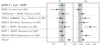 |
Fig. 6. Joint-probe comparison of S8 and Ωm constraints. Our fiducial results (KiDS 2 × 2 pt +SMF) can be compared to: a similar 2 × 2 pt +SMF analysis from the SDSS (Cacciato et al. 2013); a series of 2 × 2 pt studies that includes the latest results from DES (Porredon et al. 2022; Pandey et al. 2022) and the HSC survey (Miyatake et al. 2022b); and 3 × 2 pt analyses from KiDS with BOSS (Heymans et al. 2021) and DES (DES Collaboration 2022). The last entry shows the Planck Collaboration VI (2020, TT,TE,EE+lowE) constraints. Our results are consistent with all studies, including Planck Collaboration VI (2020), although we find a mild tension between our S8 constraints and those from Planck, at the level of 1.9σ. |
The constraining power of the KiDS 2 × 2 pt+SMF analysis in the S8 − Ωm plane is the same as that of the 3 × 2pt studies from DES Collaboration (2022), with ![Mathematical equation: $ \sigma^{S_8}\sigma^{\Omega_{\mathrm{m}}}_{[\mathrm{DES\, 3 \times 2pt}]} / \sigma^{S_8}\sigma^{\Omega_{\mathrm{m}}}_{[\mathrm{KiDS\, 2\times 2\,pt+SMF}]} = 0.97 $](/articles/aa/full_html/2023/07/aa45158-22/aa45158-22-eq113.gif) . This may be surprising given the five-fold increase in area for DES relative to KiDS, and the addition of the cosmic shear probe in the 3 × 2pt analysis. This comparison therefore highlights the significant constraining power from the inclusion of non-linear scales in the 2 × 2 pt+SMF analysis that are excluded from the DES 3 × 2pt analysis. Comparing KiDS 2 × 2 pt+SMF constraints to the KiDS with the BOSS 3 × 2pt analysis (Heymans et al. 2021), we first review the BOSS spectroscopic clustering constraints where
. This may be surprising given the five-fold increase in area for DES relative to KiDS, and the addition of the cosmic shear probe in the 3 × 2pt analysis. This comparison therefore highlights the significant constraining power from the inclusion of non-linear scales in the 2 × 2 pt+SMF analysis that are excluded from the DES 3 × 2pt analysis. Comparing KiDS 2 × 2 pt+SMF constraints to the KiDS with the BOSS 3 × 2pt analysis (Heymans et al. 2021), we first review the BOSS spectroscopic clustering constraints where ![Mathematical equation: $ \sigma^{S_8}\sigma^{\Omega_{\mathrm{m}}}_{[\mathrm{BOSS\, 1\times 2pt}]} / \sigma^{S_8}\sigma^{\Omega_{\mathrm{m}}}_{[\mathrm{KiDS\, 2\times 2\,pt+SMF}]} = 1.03 $](/articles/aa/full_html/2023/07/aa45158-22/aa45158-22-eq114.gif) . Finding the same constraining power between these analyses may again be surprising, given the nine-fold increase in area for BOSS relative to KiDS. As such, it demonstrates the significant constraining power from non-linear scales when the galaxy bias can be constrained using galaxy-galaxy lensing and galaxy abundance. Comparing to the full 3 × 2 pt analysis we find
. Finding the same constraining power between these analyses may again be surprising, given the nine-fold increase in area for BOSS relative to KiDS. As such, it demonstrates the significant constraining power from non-linear scales when the galaxy bias can be constrained using galaxy-galaxy lensing and galaxy abundance. Comparing to the full 3 × 2 pt analysis we find ![Mathematical equation: $ \sigma^{S_8}\sigma^{\Omega_{\mathrm{m}}}_{[\mathrm{KiDS+BOSS\, 3\times 2\,pt}]} / \sigma^{S_8}\sigma^{\Omega_{\mathrm{m}}}_{[\mathrm{KiDS\, 2\times 2\,pt+SMF}]} = 0.39 $](/articles/aa/full_html/2023/07/aa45158-22/aa45158-22-eq115.gif) , where the extra constraining power in the 3 × 2 pt analysis is driven by the cosmic shear. Future studies with KiDS will combine 2 × 2 pt+SMF with cosmic shear data, including further development and validation of our adopted halo model methodology.
, where the extra constraining power in the 3 × 2 pt analysis is driven by the cosmic shear. Future studies with KiDS will combine 2 × 2 pt+SMF with cosmic shear data, including further development and validation of our adopted halo model methodology.
In Appendix E we explore a number of extensions to our fiducial analysis. In Appendix E.1 we quantify the expected contamination to our observables from intrinsic galaxy alignments and magnification. The contamination levels are found to be negligible relative to our statistical errors, justifying our choice to not account for these astrophysical effects in our model. In Appendix E.2 we demonstrate that our S8 and Ωm constraints are insensitive to our choice of prior on ns. In Appendix E.3 we quantify the bias in Ωm without the inclusion of our nuisance parameter 𝒟 to model photometric redshift dilution in our galaxy clustering measurement. In Appendix 4.4 we quantify the impact of assumptions governing the behaviour of satellite galaxies.
4.2. Large-scale analysis
Amon et al. (2022b) present a detailed analysis of the uncertainty on the amplitude of the small-scale galaxy-galaxy lensing and galaxy clustering signal for BOSS galaxies that arises from our imperfect knowledge of baryon feedback and assembly bias. They conclude that the introduction of scale cuts with rp > 5h−1 Mpc fully isolates these effects. Following the methodology in Appendix C we determine  for a large-scale only 2 × 2 pt+SMF data vector analysis, calculating the large-scale goodness of fit of our fiducial best-fit model (see Table 2) to be
 ![Mathematical equation: $ p[\chi^2 (r_{\mathrm{p}} > 5) | \nu_{\mathrm{eff}}^{r_{\mathrm{p}}>5}] = 0.19 $](/articles/aa/full_html/2023/07/aa45158-22/aa45158-22-eq117.gif) . As such, we find no sign of tension between our fiducial all-scale analysis and a restricted large-scale analysis.
. As such, we find no sign of tension between our fiducial all-scale analysis and a restricted large-scale analysis.
The majority of the information in our (rp > 5) data vector comes from the SMF as there are only 4 highly correlated data points remaining in the ESD and wp measurements, per stellar mass bin. We found that a full likelihood analysis of the (rp > 5) data vector was unable to converge in our highly flexible 17-parameter model space. Where larger scales are used exclusively, either more precise data or the use of a less flexible model is necessary (such as in More 2013; Miyatake et al. 2022b; Amon et al. 2022b, amongst others). The extra flexibility afforded in our model is, however, essential when analysing small scales in order to capture baryonic effects (Debackere et al. 2020, 2021).
4.3. Galaxy-halo connection
The powerful aspect of the method used in this work is that it is able to simultaneously constrain both cosmological parameters as well as the halo occupation statistics. The full results are listed in Table 2 and the marginalised posterior distributions of all the parameters are shown in Fig. E.2. The HOD parameters are tightly constrained, with some strong degeneracies between the parameters M0, M1 and γ1 that govern the characteristic mass of the stellar-to-halo mass relation knee and the high mass slope of centrals, and between the b0 and b1 parameters, which govern the normalisation of the satellite CSMF. The first degeneracy is somewhat expected given the data, as the SMF at the high mass end is highly uncertain and dominated by the Eddington bias. The second degeneracy also arises from the fact that both parameters compete for the overall normalisation of the satellite CSMF.
We find the parameters of our HOD model to be in good agreement with the previous studies using GAMA-like galaxies (van Uitert et al. 2016; Dvornik et al. 2018; Bilicki et al. 2021). In order to show the agreement in a more intuitive way, we take the parameters of the stellar-to-halo mass relation and combine them using the same functional form (Eq. (19)), which results in the relation shown in Fig. 7. In the same figure we show good agreement with the results from van Uitert et al. (2016), where the HOD parameters were constrained using galaxy-galaxy lensing combined with a SMF for KiDS and GAMA data, adopting a fixed Planck cosmology. We also find qualitative agreement with constraints from abundance matching to numerical simulations (Moster et al. 2013) and constraints from a 2 × 2 pt+SMF analysis of COSMOS with a fixed WMAP5 cosmology (Leauthaud et al. 2012, note here we compare to constraints from the most similar 0.22 < z < 0.48 COSMOS sample) as well as the CFHTLenS/VIPERS analysis by Coupon et al. (2015). We find our constraints on the scatter of the central CSMF, σc, and the low mass end slope of the satellites, αs, to be in agreement with Yang et al. (2009), Cacciato et al. (2013), van Uitert et al. (2016), Dvornik et al. (2018), and Bilicki et al. (2021). The Eddington bias at the high mass end is captured by the σc parameter, leaving the other parameters mostly unaffected.
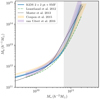 |
Fig. 7. Stellar-to-halo mass relation, as defined by Eq. (19), using the best-fit HOD parameters from our 2 × 2 pt+SMF analysis (blue). The result can be compared to results from Leauthaud et al. (2012, green), Moster et al. (2013, black), Coupon et al. (2015, orange), and van Uitert et al. (2016, purple). The grey area shows the range in stellar masses where the obtained stellar-to-halo mass relation is extrapolated beyond the range of median stellar masses used in this analysis. |
We account for the impact of baryon feedback in our model by allowing for freedom in the normalisation of the mass-concentration relation for both the haloes, fh, and the satellite galaxy distribution, fs (Eq. (15)). With these independent free parameters we can capture the expected small-scale baryon feedback power suppression shown in hydrodynamical simulations (Debackere et al. 2021; Amon et al. 2022b). We find fh and fs to be consistent with 1, with a preference for lower values, with 1σ lower limits fh > 0.65 and fs > 0.38. Our results are consistent with Viola et al. (2015), indicating that the concentrations of real haloes and satellite distributions are smaller than the haloes in dark-matter-only simulations (see also Debackere et al. 2020, 2021). Future work will compare direct measurements from hydrodynamical simulations (e.g. McCarthy et al. 2017) with our halo model approach to account for the mass dependence of baryonic effects on the radial profiles of dark matter haloes.
4.4. Modelling satellite galaxies
In our fiducial model we used the findings of Dvornik et al. (2018) that showed that the occupation distribution of satellite galaxies does not follow a Poisson distribution, and that generally the parameter 𝒫 (Eq. (25)) is not unity, with our fiducial run preferring a sub-Poissonian behaviour. Following Cacciato et al. (2013), we quantify the impact of removing this flexibility in the model, by fixing the parameter 𝒫 to unity,
 (51)
(51)
thus assuming that the satellite galaxies obey the Poisson distribution. We run another set of MCMC chains using the same setup as in the fiducial case, but with one fewer parameter to constrain. The resulting constraints are shown in Fig. E.2, with marginalised constraints quoted in Table E.1. We find significant shifts for the two main cosmological parameters with Ωm = 0.330±0.019 and  and a formally acceptable fit with p(χ2|νeff) = 0.02 for the whole data vector. In this case we find that the fixed Poisson parameter non-trivially affects the other parameters governing the satellites in the halo model. Specifically the normalisation of the satellite conditional stellar mass function, b0 and b1, shifts, and these parameters are in turn non-trivially correlated with the main cosmological parameters. Cacciato et al. (2013) argues that flexibility in the form of the satellite galaxy model is critically important in order to both constrain the galaxy bias (Cacciato et al. 2012; Dvornik et al. 2018; Asgari et al. 2021a), and to obtain unbiased cosmological parameters.
There are several reasons to reject the results of our Poissonian satellite distribution model analysis. First, whilst we find an acceptable fit of the 𝒫 = 1 model to our full 2 × 2 pt+SMF data vector, there is an unacceptable fit to the wp part of the data vector, with ![Mathematical equation: $ p[\chi^2(\mathit{w}_{\mathrm{p}}) | \nu_{\mathrm{eff}}^{\mathit{w}_{\mathrm{p}}}] \sim 10^{-4} $](/articles/aa/full_html/2023/07/aa45158-22/aa45158-22-eq120.gif) . Secondly, there is observational evidence from the GAMA group catalogue (Robotham et al. 2011) that for haloes with masses below 1013 h−1 M⊙, the number of satellites exhibit sub-Poisson behaviour, where in Fig. 8 we measure 𝒫(M) as a function of the dynamical mass Mdyn (Driver et al. 2022). We relate the parameter 𝒫 with the observed mean and variance of the number of GAMA group members in narrow bins of dynamical mass, Mdyn, as
. Secondly, there is observational evidence from the GAMA group catalogue (Robotham et al. 2011) that for haloes with masses below 1013 h−1 M⊙, the number of satellites exhibit sub-Poisson behaviour, where in Fig. 8 we measure 𝒫(M) as a function of the dynamical mass Mdyn (Driver et al. 2022). We relate the parameter 𝒫 with the observed mean and variance of the number of GAMA group members in narrow bins of dynamical mass, Mdyn, as
![Mathematical equation: $$ \begin{aligned} \mathcal{P} (M_{\mathrm{dyn} }) = \left( \frac{\mathrm{Var} [N_{\mathrm{s} }\vert M_{\mathrm{dyn} }]}{\langle N_{\mathrm{s} }\vert M_{\mathrm{dyn} } \rangle } - 1 \right) \frac{1}{\langle N_{\mathrm{s} }\vert M_{\mathrm{dyn} } \rangle } + 1. \end{aligned} $$](/articles/aa/full_html/2023/07/aa45158-22/aa45158-22-eq121.gif) (52)
(52)
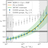 |
Fig. 8. Poissonian parameter, 𝒫 (Eq. (52)), as a function of dynamical group mass, Mdyn, for GAMA galaxy groups with three or more members (blue), and groups with five or more members (white). The orange and green lines show the best-fit power law (Eq. (53)) to the GAMA/2 × 2 pt+SMF data, with the green-shaded region showing the uncertainty on the 2 × 2 pt+SMF fit. The fiducial, single value model for 𝒫 is shown with the grey horizontal band. With the wiggly grey-shaded areas, we show the approximate range of dynamical group masses that are outside the halo mass range of our analysis. |
Here the mean ⟨Ns|Mdyn⟩ and variance Var[Ns|Mdyn] are directly obtained from the GAMA groups catalogue, where we select groups with the number of members that is equal to or larger than 3 (Robotham et al. 2011). We find the satellite distribution to be sub-Poissonian for Mdyn < 1013 h−1 M⊙, ranging from 𝒫(Mdyn) = 0.15 at Mdyn = 1011 h−1 M⊙, to 𝒫(Mdyn) = 0.76 at Mdyn = 1013 h−1 M⊙, (shown blue in Fig. 8). Assuming the GAMA dynamical mass is a reasonable estimate of the halo mass Mh, using Fig. 7 to define our stellar mass range, we expect the satellite distribution to be sub-Poissonian across the full stellar mass range of our 2 × 2 pt+SMF analysis. This sub-Poissonian behaviour is recovered in our fiducial analysis where 𝒫 = 0.403±0.029. In Dvornik et al. (2018) analysis the behaviour of satellite galaxies is recovered to be super-Poissonian, which is consistent with the trend seen in Fig. 8, as the halo masses of GAMA galaxies in that sample were above 1013 h−1 M⊙.
Finally, hydrodynamical simulations show that for haloes with masses above ∼5 × 10¹² h−1 M⊙, the number of satellites exhibit super-Poisson behaviour (Hadzhiyska et al. 2022) and for haloes with masses below ∼5 × 10¹² h−1 M⊙, the number of satellites exhibit sub-Poisson behaviour (Kravtsov et al. 2004; Jiang & van den Bosch 2017; Bhowmick et al. 2018; Beltz-Mohrmann et al. 2020). The studies from Beltz-Mohrmann et al. (2020) and Hadzhiyska et al. (2022) show a large uncertainty on the Poisson number and can be to an extent also well described by a model that assumes a Poisson distribution, while the results from Kravtsov et al. (2004), Jiang & van den Bosch (2017) and Bhowmick et al. (2018) show a clear sub-Poisson behaviour for low mass haloes, with the analysis of Jiang & van den Bosch (2017) also showing super-Poisson behaviour for high mass haloes with a transition period where satellite galaxies behave completely Poissonian. What is more, a recent analysis (Linke et al. 2022) of a semi-analytic simulation (Henriques et al. 2015) using galaxy-matter bispectrum shows that parameter 𝒫 indeed varies from sub-Poisson behaviour to super-Poisson behaviour as halo mass increases, and it seems to be furthermore dependant on the stellar mass as well (Appendix B therein).
Given the significant impact of the form of the satellite galaxy model on our cosmology constraints, we explore the satellite distribution further, noting that Fig. 8 reveals a strong mass dependence that is missing from our fiducial model. We determined the impact of neglecting this mass dependence in our analysis by including an explicit halo mass dependence on the Poisson parameter, 𝒫. We fitted a power law function to the GAMA data as
 (53)
(53)
finding A = 0.43, B = 0.39 and Mpiv = 12.54 when M = Mdyn (shown in orange in Fig. 8). In our extended 2 × 2 pt+SMF analysis, we modelled 𝒫(M) using Eq. (53), fixing the normalisation A and slope B of the power law to the GAMA best-fit values. We treat Mpiv as a free parameter, however, to account for the uncertainty in the relationship between the GAMA dynamical mass, Mdyn, and the true lensing halo mass used in the halo model. The best-fit Mpiv from the 2 × 2 pt+SMF is nevertheless found to be in good agreement with the GAMA fit (shown in green in Fig. 8).
Using the 𝒫(M) model, we obtained the parameter constraints listed in Table 2 and shown in Fig. E.2. We find a good fit of the model to the data with p(χ2|νeff) = 0.19. All the parameters are consistent with the constraints from our fiducial analysis that assumes no mass dependence. We find a preference for lower values for the two primary cosmological parameters, with  and
and  corresponding to a 1.3σ and 0.7σ difference from the fiducial result (see also Fig. E.1).
This extension analysis shows that our results are sensitive to how we modelled the mass dependence of the satellite group distribution, at an acceptable level of ∼1σ in our primary cosmological parameters. We chose not to use this extended 𝒫(M) model in our fiducial analysis, as in Fig. 8, we show how sensitive the GAMA-measured 𝒫(Mdyn) relationship is to the group selection criteria. We find that the behaviour changes when groups are defined with a number of members that is equal or larger than five (white data points, compared to the blue data points for our original selection criteria). In future higher signal-to-noise studies we will explore keeping the parameters A and B free in the 𝒫(M) model, and implement a more complex model that uses the non-Poisson behaviour directly in the definition of the HOD (for instance a negative binomial distribution as shown in Boylan-Kolchin et al. 2010). Further considerations need to be taken into account for possible stellar mass dependence of the Poisson parameter 𝒫 (Linke et al. 2022).
5. Discussion and conclusions
In this paper we have combined measurements of galaxy clustering, galaxy-galaxy lensing, and galaxy abundances in the form of the SMF in order to simultaneously set constraints on cosmological parameters and galaxy bias. Using a flexible halo model, we analysed the fourth data release of the KiDS (KiDS-1000; Kuijken et al. 2019), where the source sample, used to measure the galaxy-galaxy lensing signal, has undergone a rigorous study to assess its robustness and accuracy (Asgari et al. 2021b; Giblin et al. 2021; Hildebrandt et al. 2021). For our lens sample we used the KiDS-Bright sample (Bilicki et al. 2021), whose selection was calibrated against a complete and representative spectroscopic sample from the GAMA survey (Driver et al. 2011), with the photometric redshifts calibrated using a neural network (ANNz2; Sadeh et al. 2016). The resulting accuracy of the estimated redshifts for the KiDS-Bright sample is sufficient for galaxy-galaxy lensing and galaxy clustering studies.
We used the halo model to analyse our data, building upon the cosmological analyses presented in Cacciato et al. (2013) and More et al. (2015). We used a single halo occupation model to compute the clustering of galaxies, the galaxy-galaxy lensing signal (Guzik & Seljak 2002; Yoo et al. 2006; Cacciato et al. 2009), and the galaxy abundances (van den Bosch et al. 2013; Cacciato et al. 2013). This model is shown to be able to simultaneously constrain cosmology and halo occupation statistics, as well as constrain extensions to the standard ΛCDM cosmologies, such as the equation of state of dark energy and neutrino mass (More et al. 2013; Krause & Eifler 2017).
We have improved upon previous studies by (i) using a more accurate N-body simulation calibrated analytical model, taking halo exclusion, scale dependence, and the non-linear nature of halo bias into account (Mead & Verde 2021; Mahony et al. 2022), (ii) using the latest lensing and clustering data from a single survey (KiDS-1000), and (iii) using a full analytical covariance matrix that accounts for cross-covariance between all observables and in particular the cross-covariance between the SMF and two-point statistics.
We adopted a Bayesian approach to constrain our model parameters, using the MCMC to probe the posterior distributions. For a flat ΛCDM cosmology, we find 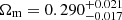 and
and 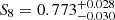 , which is consistent with and comparable to constraints from 3 × 2 pt studies that also include a cosmic shear observable (Heymans et al. 2021; DES Collaboration 2022). Our results follow the trend seen in other lensing studies of a tension in S8 when compared to Planck Collaboration VI (2020). Using the Hellinger distance as a tension metric, this difference is at the 1.9σ level for our 2 × 2 pt+SMF analysis. We find that our constraints are sensitive, at the ∼1σ level (in S8), to how we choose to model the mass dependence of the satellite distribution within the halo model. This aspect of our analysis will require further development in future higher signal-to-noise studies.
Combining galaxy clustering and galaxy-galaxy lensing with cosmic shear measurements has been a standard approach for large-scale structure analyses in recent years (van Uitert et al. 2018; Joudaki et al. 2017; Abbott et al. 2018; DES Collaboration 2022; Heymans et al. 2021). We anticipate that combining our halo model approach with cosmic shear data will allow for additional constraints on astrophysical systematics arising from the intrinsic alignment (IA) of galaxies and baryon feedback. So far, IAs in cosmic shear analysis have been included using either a non-linear modification of the linear alignment model (NLA; Bridle & King 2007) or a perturbation theory approach (TATT; Blazek et al. 2019). For a consistent halo model approach, this effect could also be modelled within the framework adopted in this analysis (e.g. Fortuna et al. 2021). In this analysis we have varied the halo concentration parameter to account for baryon feedback. With additional data, a more complex halo model that would allow for the inclusion of gas observables could be adopted to constrain baryon feedback through the Sunyaev-Zeldovich effect (Mead et al. 2020; Tröster et al. 2022). The flexibility of the halo model also allows for extensions to the underlying cosmological model without having to employ a myriad of costly simulations to cover a large range of parameters (Cataneo et al. 2019). We therefore see a significant role for our adopted methodology in future cosmological analyses of upcoming large-scale structure surveys.
The standard halo model of dark matter haloes estimates the true power spectrum to within 20% accuracy on non-linear scales (Mead et al. 2015).
Our prior range is larger than the range of available nodes in the DARKQUEST emulator. Due to the iterative updates to the βNL estimation and the quick convergence we find towards parameters within the emulator’s range, this does not pose an issue.
The moves are further defined in the documentation of the emcee package at https://emcee.readthedocs.io.
We define an acceptable fit when p(χ2|νeff)≥0.003, corresponding to less than a 3σ event, (see the discussion in Heymans et al. 2021). We note that DES Collaboration (2022) define a more stringent requirement where p(χ2|νeff)≥0.01. We find the goodness of fit for our 2 × 2 pt+SMF analysis, and each individual component of the data vector, to be acceptable given both these definitions.
Porredon et al. (2022), Pandey et al. (2022) also explore small-scale 2 × 2pt analyses using non-linear galaxy bias models, finding a 20–30% gain in cosmological constraining power.
We note that our simulation approach finds a slightly larger νeff compared to the estimation using the Raveri & Hu (2019) approach, for which we find νeff = 138.5,
Acknowledgments
We thank Andrew Hearin for useful discussion on modelling the non-Poissonian behaviour of satellite galaxies, and the anonymous referee for the helpful comments and constructive remarks on this manuscript. We acknowledge support from the European Research Council under grants 770935 (AD, CM, HHi, RR, AHW) and 647112 (CH, MA), and the UK Science and Technology Facilities Council (STFC) under grants ST/V000594/1 (CH, MA) and ST/V000780/1 (BJ). HHi is further supported by a Heisenberg grant of the Deutsche Forschungsgemeinschaft (Hi 1495/5-1). CH and AM acknowledge support from the Max Planck Society and the Alexander von Humboldt Foundation in the framework of the Max Planck-Humboldt Research Award endowed by the Federal Ministry of Education and Research. MB is supported by the Polish National Science Center through grants no. 2020/38/E/ST9/00395, 2018/30/E/ST9/00698, 2018/31/G/ST9/03388 and 2020/39/B/ST9/03494, and by the Polish Ministry of Science and Higher Education through grant DIR/WK/2018/12. EC and HJ acknowledges support from the Delta ITP consortium, a program of the Netherlands Organisation for Scientific Research (NWO) that is funded by the Dutch Ministry of Education, Culture and Science (OCW), project number 24.001.027. HHo acknowledges support from Vici grant 639.043.512, financed by the Netherlands Organisation for Scientific Research (NWO). KK acknowledges support from the Royal Society and Imperial College. HM was supported in part by World Premier International Research Center Initiative (WPI Initiative), MEXT, Japan, by JSPS KAKENHI Grant Numbers 20H01932, by JSPS Core-to-Core Program Grant Number JPJSCCA20200002, and by Japan Science and Technology Agency (JST) CREST JPMHCR1414 and JST AIP Acceleration Research Grant Number JP20317829, Japan. TN is supported in part by MEXT/JSPS KAKENHI Grant Numbers P19H00677, P20H05861, JP21H01081, JP22K0363, and Japan Science and Technology Agency (JST) AIP Acceleration Research Grant Number JP20317829. Based on observations made with ESO Telescopes at the La Silla Paranal Observatory under programme IDs 177.A-3016, 177.A-3017, 177.A-3018 and 179.A-2004, and on data products produced by the KiDS consortium. The KiDS production team acknowledges support from: Deutsche Forschungsgemeinschaft, ERC, NOVA and NWO-M grants; Target; the University of Padova, and the University Federico II (Naples). This work has made use of Python (http://www.python.org), including the packages numpy (http://www.numpy.org), scipy (http://www.scipy.org), astropy (http://www.astropy.org Astropy Collaboration 2013, 2018), and hmf (Murray et al. 2013). Plots have been produced with matplotlib (Hunter 2007) and chainconsumer (Hinton 2016). This work has made use of CosmoHub for validation of our covariance matrices. CosmoHub has been developed by the Port d’Informació Científica (PIC), maintained through a collaboration of the Institut de Física d’Altes Energies (IFAE) and the Centro de Investigaciones Energéticas, Medioambientales y Tecnológicas (CIEMAT) and the Institute of Space Sciences (CSIC & IEEC), and was partially funded by the “Plan Estatal de Investigación Científica y Técnica y de Innovación” program of the Spanish government. Author contributions: All authors contributed to writing and development of this paper. The authorship list reflects the lead authors (AD,CH,MA,CM,BJ) followed by an alphabetical group that includes those who are key contributors to the scientific analysis.
References
- Abbott, T. M. C., Abdalla, F. B., Alarcon, A., et al. 2018, Phys. Rev. D, 98, 043526 [NASA ADS] [CrossRef] [Google Scholar]
- Alam, S., Aubert, M., Avila, S., et al. 2021, Phys. Rev. D, 103, 083533 [NASA ADS] [CrossRef] [Google Scholar]
- Amon, A., Gruen, D., Troxel, M. A., et al. 2022a, Phys. Rev. D, 105, 023514 [NASA ADS] [CrossRef] [Google Scholar]
- Amon, A., Robertson, N. C., Miyatake, H., et al. 2022b, MNRAS, 518, 477 [CrossRef] [Google Scholar]
- Arnouts, S., Cristiani, S., Moscardini, L., et al. 1999, MNRAS, 310, 540 [Google Scholar]
- Asgari, M., Friswell, I., Yoon, M., et al. 2021a, MNRAS, 501, 3003 [NASA ADS] [CrossRef] [Google Scholar]
- Asgari, M., Lin, C.-A., Joachimi, B., et al. 2021b, A&A, 645, A104 [NASA ADS] [CrossRef] [EDP Sciences] [Google Scholar]
- Astropy Collaboration (Robitaille, T. P., et al.) 2013, A&A, 558, A33 [NASA ADS] [CrossRef] [EDP Sciences] [Google Scholar]
- Astropy Collaboration (Price-Whelan, A. M., et al.) 2018, AJ, 156, 123 [Google Scholar]
- Baldry, I. K., Driver, S. P., Loveday, J., et al. 2012, MNRAS, 421, 621 [NASA ADS] [Google Scholar]
- Bartelmann, M., & Schneider, P. 2001, Phys. Rep., 340, 291 [Google Scholar]
- Beltz-Mohrmann, G. D., Berlind, A. A., & Szewciw, A. O. 2020, MNRAS, 491, 5771 [NASA ADS] [CrossRef] [Google Scholar]
- Benitez, N. 2000, ApJ, 536, 571 [CrossRef] [Google Scholar]
- Bhowmick, A. K., Campbell, D., Di Matteo, T., & Feng, Y. 2018, MNRAS, 480, 3177 [CrossRef] [Google Scholar]
- Bilicki, M., Hoekstra, H., Brown, M. J. I., et al. 2018, A&A, 616, A69 [NASA ADS] [CrossRef] [EDP Sciences] [Google Scholar]
- Bilicki, M., Dvornik, A., Hoekstra, H., et al. 2021, A&A, 653, A82 [NASA ADS] [CrossRef] [EDP Sciences] [Google Scholar]
- Blake, C., Amon, A., Asgari, M., et al. 2020, A&A, 642, A158 [NASA ADS] [CrossRef] [EDP Sciences] [Google Scholar]
- Blazek, J. A., MacCrann, N., Troxel, M. A., & Fang, X. 2019, Phys. Rev. D, 100, 103506 [NASA ADS] [CrossRef] [Google Scholar]
- Boylan-Kolchin, M., Springel, V., White, S. D. M., & Jenkins, A. 2010, MNRAS, 406, 896 [Google Scholar]
- Bridle, S., & King, L. 2007, New J. Phys., 9, 444 [Google Scholar]
- Brouwer, M. M., Oman, K. A., Valentijn, E. A., et al. 2021, A&A, 650, A113 [NASA ADS] [CrossRef] [EDP Sciences] [Google Scholar]
- Brown, M. L., Taylor, A. N., Hambly, N. C., & Dye, S. 2002, MNRAS, 333, 501 [NASA ADS] [CrossRef] [Google Scholar]
- Bruzual, G., & Charlot, S. 2003, MNRAS, 344, 1000 [NASA ADS] [CrossRef] [Google Scholar]
- Cacciato, M., van den Bosch, F. C., More, S., et al. 2009, MNRAS, 394, 929 [NASA ADS] [CrossRef] [Google Scholar]
- Cacciato, M., Lahav, O., van den Bosch, F. C., Hoekstra, H., & Dekel, A. 2012, MNRAS, 426, 566 [Google Scholar]
- Cacciato, M., van den Bosch, F. C., More, S., Mo, H., & Yang, X. 2013, MNRAS, 430, 767 [Google Scholar]
- Cacciato, M., van Uitert, E., & Hoekstra, H. 2014, MNRAS, 437, 377 [CrossRef] [Google Scholar]
- Calzetti, D., Kinney, A. L., & Storchi-Bergmann, T. 1994, ApJ, 429, 582 [Google Scholar]
- Carretero, J., Castander, F. J., Gaztañaga, E., Crocce, M., & Fosalba, P. 2015, MNRAS, 447, 646 [NASA ADS] [CrossRef] [Google Scholar]
- Cataneo, M., Lombriser, L., Heymans, C., et al. 2019, MNRAS, 488, 2121 [Google Scholar]
- Chabrier, G. 2003, ApJ, 586, L133 [NASA ADS] [CrossRef] [Google Scholar]
- Chisari, N. E., Mandelbaum, R., Strauss, M. A., Huff, E. M., & Bahcall, N. A. 2014, MNRAS, 445, 726 [NASA ADS] [CrossRef] [Google Scholar]
- Cole, S. 2011, MNRAS, 416, 739 [Google Scholar]
- Cooray, A., & Sheth, R. 2002, Phys. Rep., 372, 1 [Google Scholar]
- Coupon, J., Arnouts, S., van Waerbeke, L., et al. 2015, MNRAS, 449, 1352 [NASA ADS] [CrossRef] [Google Scholar]
- Crocce, M., Castander, F. J., Gaztañaga, E., Fosalba, P., & Carretero, J. 2015, MNRAS, 453, 1513 [NASA ADS] [CrossRef] [Google Scholar]
- Davis, M., Efstathiou, G., Frenk, C. S., & White, S. D. M. 1985, ApJ, 292, 371 [Google Scholar]
- de Jong, J., Kuijken, K., Applegate, D., et al. 2013, The Messenger, 154, 44 [NASA ADS] [Google Scholar]
- Debackere, S. N. B., Schaye, J., & Hoekstra, H. 2020, MNRAS, 492, 2285 [Google Scholar]
- Debackere, S. N. B., Schaye, J., & Hoekstra, H. 2021, MNRAS, 505, 593 [NASA ADS] [CrossRef] [Google Scholar]
- Dekel, A., & Lahav, O. 1999, ApJ, 520, 24 [Google Scholar]
- Dekel, A., & Rees, M. J. 1987, Nature, 326, 455 [NASA ADS] [CrossRef] [Google Scholar]
- DES Collaboration (Abbott, T. M. C., et al.) 2022, Phys. Rev. D, 105, 023520 [CrossRef] [Google Scholar]
- Desjacques, V., Jeong, D., & Schmidt, F. 2018, Phys. Rep., 733, 1 [Google Scholar]
- Driver, S. P., Hill, D. T., Kelvin, L. S., et al. 2011, MNRAS, 413, 971 [Google Scholar]
- Driver, S. P., Robotham, A. S. G., Obreschkow, D., et al. 2022, MNRAS, 515, 2138 [NASA ADS] [CrossRef] [Google Scholar]
- Duffy, A. R., Schaye, J., Kay, S. T., & Dalla Vecchia, C. 2008, MNRAS, 390, L64 [Google Scholar]
- Dvornik, A., Cacciato, M., Kuijken, K., et al. 2017, MNRAS, 468, 3251 [Google Scholar]
- Dvornik, A., Hoekstra, H., Kuijken, K., et al. 2018, MNRAS, 479, 1240 [Google Scholar]
- Edge, A., Sutherland, W., Kuijken, K., et al. 2013, The Messenger, 154, 32 [NASA ADS] [Google Scholar]
- Eisenstein, D. J., & Hu, W. 1998, ApJ, 496, 605 [Google Scholar]
- Farrow, D. J., Cole, S., Norberg, P., et al. 2015, MNRAS, 454, 2120 [Google Scholar]
- Fenech Conti, I., Herbonnet, R., Hoekstra, H., et al. 2017, MNRAS, 467, 1627 [NASA ADS] [Google Scholar]
- Foreman-Mackey, D., Hogg, D. W., Lang, D., & Goodman, J. 2013, PASP, 125, 306 [Google Scholar]
- Fortuna, M. C., Hoekstra, H., Joachimi, B., et al. 2021, MNRAS, 501, 2983 [NASA ADS] [CrossRef] [Google Scholar]
- Fosalba, P., Crocce, M., Gaztañaga, E., & Castander, F. J. 2015a, MNRAS, 448, 2987 [NASA ADS] [CrossRef] [Google Scholar]
- Fosalba, P., Gaztañaga, E., Castander, F. J., & Crocce, M. 2015b, MNRAS, 447, 1319 [NASA ADS] [CrossRef] [Google Scholar]
- Georgiou, C., Chisari, N. E., Fortuna, M. C., et al. 2019, A&A, 628, A31 [EDP Sciences] [Google Scholar]
- Gerbino, M., & Lattanzi, M. 2018, Front. Phys., 5 [CrossRef] [Google Scholar]
- Giblin, B., Heymans, C., Asgari, M., et al. 2021, A&A, 645, A105 [NASA ADS] [CrossRef] [EDP Sciences] [Google Scholar]
- Giocoli, C., Bartelmann, M., Sheth, R. K., & Cacciato, M. 2010, MNRAS, 408, 300 [NASA ADS] [CrossRef] [Google Scholar]
- Guzik, J., & Seljak, U. 2002, MNRAS, 335, 311 [CrossRef] [Google Scholar]
- Hadzhiyska, B., Hernquist, L., Eisenstein, D., et al. 2022, MNRAS, 14, 1 [Google Scholar]
- Hamana, T., Shirasaki, M., Miyazaki, S., et al. 2019, J. Biochem., 166, 1 [CrossRef] [Google Scholar]
- Henriques, B. M. B., White, S. D. M., Thomas, P. A., et al. 2015, MNRAS, 451, 2663 [Google Scholar]
- Heymans, C., Grocutt, E., Heavens, A., et al. 2013, MNRAS, 432, 2433 [Google Scholar]
- Heymans, C., Tröster, T., Asgari, M., et al. 2021, A&A, 646, A140 [NASA ADS] [CrossRef] [EDP Sciences] [Google Scholar]
- Hikage, C., Oguri, M., Hamana, T., et al. 2019, PASJ, 71, 1 [NASA ADS] [CrossRef] [Google Scholar]
- Hildebrandt, H., van den Busch, J. L., Wright, A. H., et al. 2021, A&A, 647, A124 [EDP Sciences] [Google Scholar]
- Hinton, S. 2016, J. Open Source Softw., 1, 45 [NASA ADS] [CrossRef] [Google Scholar]
- Hoffmann, K., Bel, J., Gaztañaga, E., et al. 2015, MNRAS, 447, 1724 [NASA ADS] [CrossRef] [Google Scholar]
- Hunter, J. D. 2007, Comput. Sci. Eng., 9, 90 [NASA ADS] [CrossRef] [Google Scholar]
- Ilbert, O., Arnouts, S., McCracken, H. J., et al. 2006, A&A, 457, 841 [NASA ADS] [CrossRef] [EDP Sciences] [Google Scholar]
- Jiang, F., & van den Bosch, F. C. 2017, MNRAS, 472, 657 [NASA ADS] [CrossRef] [Google Scholar]
- Joachimi, B., & Bridle, S. L. 2010, A&A, 523, A1 [NASA ADS] [CrossRef] [EDP Sciences] [Google Scholar]
- Joachimi, B., Mandelbaum, R., Abdalla, F. B., & Bridle, S. L. 2011, A&A, 527, A26 [NASA ADS] [CrossRef] [EDP Sciences] [Google Scholar]
- Joachimi, B., Lin, C.-A., Asgari, M., et al. 2021, A&A, 646, A129 [NASA ADS] [CrossRef] [EDP Sciences] [Google Scholar]
- Johnston, H., Wright, A. H., Joachimi, B., et al. 2021a, A&A, 648, A98 [NASA ADS] [CrossRef] [EDP Sciences] [Google Scholar]
- Johnston, H., Joachimi, B., Norberg, P., et al. 2021b, A&A, 646, A147 [NASA ADS] [CrossRef] [EDP Sciences] [Google Scholar]
- Joudaki, S., Mead, A., Blake, C., et al. 2017, MNRAS, 471, 1259 [NASA ADS] [CrossRef] [Google Scholar]
- Kaiser, N. 1987, MNRAS, 227, 1 [Google Scholar]
- Kannawadi, A., Hoekstra, H., Miller, L., et al. 2019, A&A, 624, A92 [NASA ADS] [CrossRef] [EDP Sciences] [Google Scholar]
- Krause, E., & Eifler, T. 2017, MNRAS, 470, 2100 [NASA ADS] [CrossRef] [Google Scholar]
- Kravtsov, A. V., Berlind, A. A., Wechsler, R. H., et al. 2004, ApJ, 609, 35 [Google Scholar]
- Kuijken, K. 2011, The Messenger, 146, 8 [NASA ADS] [Google Scholar]
- Kuijken, K., Heymans, C., Dvornik, A., et al. 2019, A&A, 625, A2 [NASA ADS] [CrossRef] [EDP Sciences] [Google Scholar]
- Landy, S. D., & Szalay, A. S. 1993, ApJ, 412, 64 [Google Scholar]
- Lange, J. U., Leauthaud, A., Singh, S., et al. 2021, MNRAS, 502, 2074 [CrossRef] [Google Scholar]
- Leauthaud, A., Tinker, J., Behroozi, P. S., Busha, M. T., & Wechsler, R. H. 2011, ApJ, 738, 45 [NASA ADS] [CrossRef] [Google Scholar]
- Leauthaud, A., Tinker, J., Bundy, K., et al. 2012, ApJ, 744, 159 [Google Scholar]
- Leauthaud, A., Saito, S., Hilbert, S., et al. 2017, MNRAS, 467, 3024 [Google Scholar]
- Li, R., Mo, H. J., Fan, Z., et al. 2009, MNRAS, 394, 1016 [NASA ADS] [CrossRef] [Google Scholar]
- Li, S.-S., Kuijken, K., Hoekstra, H., et al. 2021, A&A, 646, A175 [NASA ADS] [CrossRef] [EDP Sciences] [Google Scholar]
- Li, Y., Hu, W., & Takada, M. 2014, Phys. Rev. D - Part. Fields, Gravit. Cosmol., 89, 1 [Google Scholar]
- Linke, L., Simon, P., Schneider, P., et al. 2022, A&A, 665, A38 [NASA ADS] [CrossRef] [EDP Sciences] [Google Scholar]
- Mahony, C., Dvornik, A., Mead, A., et al. 2022, MNRAS, 515, 2612 [NASA ADS] [CrossRef] [Google Scholar]
- Mandelbaum, R., Seljak, U., Baldauf, T., & Smith, R. E. 2010, MNRAS, 405, 2078 [NASA ADS] [Google Scholar]
- Mandelbaum, R., Slosar, A., Baldauf, T., et al. 2013, MNRAS, 432, 1544 [NASA ADS] [CrossRef] [Google Scholar]
- Marian, L., Smith, R. E., & Angulo, R. E. 2015, MNRAS, 451, 1418 [NASA ADS] [CrossRef] [Google Scholar]
- McCarthy, I. G., Schaye, J., Bird, S., & Le Brun, A. M. C. 2017, MNRAS, 465, 2936 [Google Scholar]
- Mead, A. J., & Verde, L. 2021, MNRAS, 503, 3095 [NASA ADS] [CrossRef] [Google Scholar]
- Mead, A. J., Peacock, J. A., Heymans, C., Joudaki, S., & Heavens, A. F. 2015, MNRAS, 454, 1958 [NASA ADS] [CrossRef] [Google Scholar]
- Mead, A. J., Tröster, T., Heymans, C., Van Waerbeke, L., & McCarthy, I. G. 2020, A&A, 641, A130 [EDP Sciences] [Google Scholar]
- Miller, L., Heymans, C., Kitching, T. D., et al. 2013, MNRAS, 429, 2858 [Google Scholar]
- Miyatake, H., Kobayashi, Y., Takada, M., et al. 2022a, Phys. Rev. D, 106, 083519 [NASA ADS] [CrossRef] [Google Scholar]
- Miyatake, H., Sugiyama, S., Takada, M., et al. 2022b, Phys. Rev. D, 106, 083520 [NASA ADS] [CrossRef] [Google Scholar]
- Mo, H., van den Bosch, F., & White, S. 2010, Galaxy Formation and Evolution (Cambridge: Cambridge University Press), 810 [Google Scholar]
- More, S. 2013, ApJ, 777, L26 [NASA ADS] [CrossRef] [Google Scholar]
- More, S., van den Bosch, F. C., Cacciato, M., et al. 2013, MNRAS, 430, 747 [NASA ADS] [CrossRef] [Google Scholar]
- More, S., Miyatake, H., Mandelbaum, R., et al. 2015, ApJ, 806, 2 [CrossRef] [Google Scholar]
- Moster, B. P., Naab, T., & White, S. D. M. 2013, MNRAS, 428, 3121 [Google Scholar]
- Murray, S., Power, C., & Robotham, A. 2013, Astron. Comput., 3–4, 23 [CrossRef] [Google Scholar]
- Navarro, J. F., Frenk, C. S., & White, S. D. M. 1997, ApJ, 490, 493 [Google Scholar]
- Nishimichi, T., Takada, M., Takahashi, R., et al. 2019, ApJ, 884, 29 [NASA ADS] [CrossRef] [Google Scholar]
- Pandey, S., Krause, E., DeRose, J., et al. 2022, Phys. Rev. D, 106, 043520 [NASA ADS] [CrossRef] [Google Scholar]
- Peacock, J. A., & Smith, R. E. 2000, MNRAS, 318, 1144 [Google Scholar]
- Pielorz, J., Rödiger, J., Tereno, I., & Schneider, P. 2010, A&A, 514, A79 [NASA ADS] [CrossRef] [EDP Sciences] [Google Scholar]
- Planck Collaboration VI. 2020, A&A, 641, A6 [NASA ADS] [CrossRef] [EDP Sciences] [Google Scholar]
- Porredon, A., Crocce, M., Elvin-Poole, J., et al. 2022, Phys. Rev. D, 106, 103530 [NASA ADS] [CrossRef] [Google Scholar]
- Raveri, M., & Hu, W. 2019, Phys. Rev. D, 99, 043506 [NASA ADS] [CrossRef] [Google Scholar]
- Robotham, A. S. G., Norberg, P., Driver, S. P., et al. 2011, MNRAS, 416, 2640 [NASA ADS] [CrossRef] [Google Scholar]
- Sadeh, I., Abdalla, F. B., & Lahav, O. 2016, PASP, 128, 104502 [NASA ADS] [CrossRef] [Google Scholar]
- Sánchez, A. G., Scoccimarro, R., Crocce, M., et al. 2017, MNRAS, 464, 1640 [Google Scholar]
- Saunders, W., Rowan-Robinson, M., Lawrence, A., et al. 1990, MNRAS, 242, 318 [Google Scholar]
- Schaan, E., Takada, M., & Spergel, D. N. 2014, Phys. Rev. D, 90, 123523 [NASA ADS] [CrossRef] [Google Scholar]
- Schaller, M., Frenk, C. S., Bower, R. G., et al. 2015, MNRAS, 451, 1247 [Google Scholar]
- Schlafly, E. F., & Finkbeiner, D. P. 2011, ApJ, 737, 103 [Google Scholar]
- Schlegel, D. J., Finkbeiner, D. P., & Davis, M. 1998, ApJ, 500, 525 [Google Scholar]
- Schmidt, M. 1968, ApJ, 151, 393 [Google Scholar]
- Schneider, A., & Teyssier, R. 2015, J. Cosmol. Astropart. Phys., 2015, 049 [CrossRef] [Google Scholar]
- Scoccimarro, R., Sheth, R. K., Hui, L., & Jain, B. 2001, ApJ, 546, 20 [NASA ADS] [CrossRef] [Google Scholar]
- Scolnic, D. M., Jones, D. O., Rest, A., et al. 2018, ApJ, 859, 101 [NASA ADS] [CrossRef] [Google Scholar]
- Secco, L. F., Samuroff, S., Krause, E., et al. 2022, Phys. Rev. D, 105, 023515 [NASA ADS] [CrossRef] [Google Scholar]
- Seljak, U. 2000, MNRAS, 318, 203 [Google Scholar]
- Seljak, U., Makarov, A., Mandelbaum, R., et al. 2005, Phys. Rev. D, 71, 043511 [Google Scholar]
- Simon, P., & Hilbert, S. 2018, A&A, 613, A15 [NASA ADS] [CrossRef] [EDP Sciences] [Google Scholar]
- Singh, S., Mandelbaum, R., Seljak, U., Slosar, A., & Vazquez Gonzalez, J. 2017, MNRAS, 471, 3827 [Google Scholar]
- Smith, R. E. 2012, MNRAS, 426, 531 [Google Scholar]
- Takada, M., & Bridle, S. 2007, New J. Phys., 9, 446 [NASA ADS] [CrossRef] [Google Scholar]
- Takada, M., & Hu, W. 2013, Phys. Rev. D - Part. Fields, Gravit. Cosmol., 87, 1 [Google Scholar]
- Taylor, E. N., Hopkins, A. M., Baldry, I. K., et al. 2011, MNRAS, 418, 1587 [Google Scholar]
- Tinker, J. L., Weinberg, D. H., Zheng, Z., & Zehavi, I. 2005, ApJ, 631, 41 [Google Scholar]
- Tinker, J. L., Robertson, B. E., Kravtsov, A. V., et al. 2010, ApJ, 724, 878 [NASA ADS] [CrossRef] [Google Scholar]
- Tröster, T., Asgari, M., Blake, C., et al. 2021, A&A, 649, A88 [NASA ADS] [CrossRef] [EDP Sciences] [Google Scholar]
- Tröster, T., Mead, A. J., Heymans, C., et al. 2022, A&A, 660, A27 [CrossRef] [EDP Sciences] [Google Scholar]
- Unruh, S., Schneider, P., Hilbert, S., et al. 2020, A&A, 638, A96 [NASA ADS] [CrossRef] [EDP Sciences] [Google Scholar]
- van den Bosch, F. C., More, S., Cacciato, M., Mo, H., & Yang, X. 2013, MNRAS, 430, 725 [NASA ADS] [CrossRef] [Google Scholar]
- van den Busch, J. L., Wright, A. H., Hildebrandt, H., et al. 2022, A&A, 664, A170 [NASA ADS] [CrossRef] [EDP Sciences] [Google Scholar]
- van Uitert, E., Cacciato, M., Hoekstra, H., et al. 2016, MNRAS, 459, 3251 [Google Scholar]
- van Uitert, E., Joachimi, B., Joudaki, S., et al. 2018, MNRAS, 476, 4662 [NASA ADS] [CrossRef] [Google Scholar]
- Viola, M., Cacciato, M., Brouwer, M., et al. 2015, MNRAS, 452, 3529 [NASA ADS] [CrossRef] [Google Scholar]
- Wang, L., Farrah, D., Oliver, S. J., et al. 2013, MNRAS, 431, 648 [Google Scholar]
- Wang, Y., Vogelsberger, M., Xu, D., et al. 2020, MNRAS, 491, 5188 [Google Scholar]
- Wechsler, R. H., & Tinker, J. L. 2018, ARA&A, 56, 435 [NASA ADS] [CrossRef] [Google Scholar]
- Weigel, A. K., Schawinski, K., & Bruderer, C. 2016, MNRAS, 459, 2150 [NASA ADS] [CrossRef] [Google Scholar]
- Wibking, B. D., Salcedo, A. N., Weinberg, D. H., et al. 2019, MNRAS, 484, 989 [NASA ADS] [CrossRef] [Google Scholar]
- Wright, A. H., Robotham, A. S. G., Bourne, N., et al. 2016, MNRAS, 460, 765 [Google Scholar]
- Wright, A. H., Robotham, A. S. G., Driver, S. P., et al. 2017, MNRAS, 470, 283 [NASA ADS] [CrossRef] [Google Scholar]
- Wright, A. H., Driver, S. P., & Robotham, A. S. G. 2018, MNRAS, 480, 3491 [Google Scholar]
- Wright, A. H., Hildebrandt, H., Kuijken, K., et al. 2019, A&A, 632, A34 [NASA ADS] [CrossRef] [EDP Sciences] [Google Scholar]
- Wright, A. H., Hildebrandt, H., van den Busch, J. L., et al. 2020, A&A, 640, L14 [NASA ADS] [CrossRef] [EDP Sciences] [Google Scholar]
- Yang, X., Mo, H. J., & van den Bosch, F. C. 2008, ApJ, 676, 248 [Google Scholar]
- Yang, X., Mo, H. J., & van den Bosch, F. C. 2009, ApJ, 695, 900 [Google Scholar]
- Yoo, J., Tinker, J. L., Weinberg, D. H., et al. 2006, ApJ, 652, 26 [NASA ADS] [CrossRef] [Google Scholar]
- Yoon, M., James Jee, M., Anthony Tyson, J., et al. 2019, ApJ, 870, 111 [Google Scholar]
- Zehavi, I., Zheng, Z., Weinberg, D. H., et al. 2011, ApJ, 736, 59 [NASA ADS] [CrossRef] [Google Scholar]
- Zheng, Z., Berlind, A. A., Weinberg, D. H., et al. 2005, ApJ, 633, 791 [NASA ADS] [CrossRef] [Google Scholar]
Appendix A: Stellar mass function covariance matrix
We derive the covariance of the SMF in direct analogy to the flux-limited case considered in Smith (2012), but neglect the halo occupation variance contribution because it was demonstrated to be always subdominant (Smith 2012). To simplify the expression we neglect the mapping from true stellar mass to observed stellar mass, where the corresponding integrations would appear explicitly as this relation is expected to be fairly tight. The SMF covariance is composed of a shot noise and super-sample covariance (SSC) contribution,
![Mathematical equation: $$ \begin{aligned} \mathrm{Cov} \left[\Phi _{\mu }^{i}, \Phi _{\nu }^{j}\right] = \mathrm{Cov} ^{\mathrm{SN} }\left[\Phi _{\mu }^{i}, \Phi _{\nu }^{j}\right] + \mathrm{Cov} ^{\mathrm{SSC} }\left[\Phi _{\mu }^{i}, \Phi _{\nu }^{j}\right]\,, \end{aligned} $$](/articles/aa/full_html/2023/07/aa45158-22/aa45158-22-eq127.gif) (A.1)
(A.1)
with
![Mathematical equation: $$ \begin{aligned} \mathrm{Cov} ^{\mathrm{SN} }\left[\Phi _{\mu }^{i}, \Phi _{\nu }^{j}\right] = \delta _{i,j}\,\delta _{\mu ,\nu } \frac{\Phi _{\mu }^{i}}{\Delta M_{\star } V_{\mathrm{max} ,\mu }^{i}}\,, \end{aligned} $$](/articles/aa/full_html/2023/07/aa45158-22/aa45158-22-eq128.gif) (A.2)
(A.2)
where  and
and  are the shorthands for the SMF and Vmax of stellar mass bin μ and generally a tomographic bin i. We define
![Mathematical equation: $$ \begin{aligned} \widetilde{\Phi }_{\mu } = \int _{0}^{\infty } \Phi (M_{\star , \mu } \vert M, [z]) \, n(M, z)\,b_{\mathrm{h} }(M,z) \, \mathrm{d} M\,. \end{aligned} $$](/articles/aa/full_html/2023/07/aa45158-22/aa45158-22-eq131.gif) (A.3)
(A.3)
Using this, the SSC terms are given by
![Mathematical equation: $$ \begin{aligned} \mathrm{Cov} ^{\mathrm{SSC} }\left[\Phi _{\mu }^{i}, \Phi _{\nu }^{j}\right] = \frac{A_{\mathrm{survey} }^{2}\, f^{i} f^{j}}{V_{\mathrm{max} ,\mu }^{i}\, V_{\mathrm{max} ,\nu }^{j}} \int \mathrm{d} \chi \frac{p^{i}(\chi )}{p_{\mathrm{tot} }(\chi )} \frac{p^{j}(\chi )}{p_{\mathrm{tot} }(\chi )}\, f^{2}_{K}(\chi )\, \sigma ^{2}_{\mathrm{s} }(\chi )\,\widetilde{\Phi }_{\mu }[z(\chi )]\,\widetilde{\Phi }_{\mu }[z(\chi )] \,, \end{aligned} $$](/articles/aa/full_html/2023/07/aa45158-22/aa45158-22-eq132.gif) (A.4)
(A.4)
where  is the variance of density fluctuations within the angular survey window (see Appendix E of Joachimi et al. (2021) for definition), pi are the tomographic bin-wise redshift distributions, ptot the overall redshift distribution for all galaxies in the sample and/or survey, fK the comoving angular diameter distance, χ the comoving radial distance and fi the fraction of galaxies in bin i relative to all galaxies. Asurvey is the survey area.
The cross-variance is derived in close analogy to Takada & Bridle (2007), with the consistency checks by Schaan et al. (2014). The cross-variance receives contributions from two terms,
![Mathematical equation: $$ \begin{aligned} \mathrm{Cov} \left[\Phi _{\mu }^{i}, \mathcal{O} ^{jl}(r_{\mathrm{p} })\right] = \mathrm{Cov} ^{\mathrm{CV} }\left[\Phi _{\mu }^{i}, \mathcal{O} ^{jl}(r_{\mathrm{p} })\right] + \mathrm{Cov} ^{\mathrm{SSC} }\left[\Phi _{\mu }^{i}, \mathcal{O} ^{jl}(r_{\mathrm{p} })\right]\,, \end{aligned} $$](/articles/aa/full_html/2023/07/aa45158-22/aa45158-22-eq134.gif) (A.5)
(A.5)
a cosmic variance (CV) and a SSC term, respectively. Here we determine the cross-variance with a projected two-point function, 𝒪jl(rp), of either WP (wp(r)) or ESD (ΔΣ(r)) in bins j and l, respectively. The CV contribution is a three-point correlation given by
![Mathematical equation: $$ \begin{aligned} \mathrm{Cov} ^{\mathrm{CV} }\left[\Phi _{\mu }^{i}, \mathcal{O} ^{jl}(r_{\mathrm{p} })\right] = \overline{\rho }_{\mathrm{x} } f^{i} \int \mathrm{d} \chi \frac{p^{i}(\chi )}{p_{\mathrm{tot} }(\chi )} \int {\mathrm{d}k\,k \over 2 \pi } J_{\mathrm{x} }(kr_{\mathrm{p}})\, \left(nB_{\mathrm{cmm} }\right)_{\mu }^{jl} \left[k, z(\chi )\right] \,, \end{aligned} $$](/articles/aa/full_html/2023/07/aa45158-22/aa45158-22-eq135.gif) (A.6)
(A.6)
where  and Jx = J0 in the case when observable is wp, and
  and Jx = J2 in the case when observable is ΔΣ. Jn are Bessel functions of the nth kind. Here we have defined the count-matter cross-bispectrum (evaluated for a collapsed triangle) in close analogy to Takada & Bridle (2007). It can be expressed in the halo model formalism as
![Mathematical equation: $$ \begin{aligned} \left(nB_{\mathrm{cmm} }\right)_{\mu } \left(k, z\right)&= \int \mathrm{d} M \, n(M,z) \, \Phi (M_{\star , \mu } \vert M, [z]) \, \left({M \over \overline{\rho }_{\mathrm{m} }}\right)^{2} \, \tilde{u}^{2}_{\mathrm{h} }(k \vert M) \\ \nonumber&+ 2P_{\mathrm{lin} }(k,z) \int \mathrm{d} M \, n(M,z) \, \Phi (M_{\star , \mu } \vert M, [z]) \, b_{\mathrm{h} }(M,z) {M \over \overline{\rho }_{\mathrm{m} }} \, \tilde{u}_{\mathrm{h} }(k \vert M) \int \mathrm{d} M^{\prime } \, n(M^{\prime },z) \, b_{\mathrm{h} }(M^{\prime },z) {M^{\prime } \over \overline{\rho }_{\mathrm{m} }} \, \tilde{u}_{\mathrm{h} }(k \vert M^{\prime })\,. \end{aligned} $$](/articles/aa/full_html/2023/07/aa45158-22/aa45158-22-eq138.gif) (A.7)
(A.7)
Finally, the SSC term reads
![Mathematical equation: $$ \begin{aligned} \mathrm{Cov} ^{\mathrm{SSC} }\left[\Phi _{\mu }^{i}, \mathcal{O} ^{jl}(r_{\mathrm{p} })\right] = \overline{\rho }_{\mathrm{x} } A_{\mathrm{survey} } f^{i} \int \mathrm{d} \chi \frac{p^{i}(\chi )}{p_{\mathrm{tot} }(\chi )} \int {\mathrm{d}k\,k \over 2 \pi } J_{\mathrm{x} }(kr_{\mathrm{p}})\, \frac{\partial P_{\mathrm{xy} }^{jl}(k, z(\chi ))}{\partial \delta _{\mathrm{b} }}\, \sigma ^{2}_{\mathrm{s} }(\chi )\, \widetilde{\Phi }_{\mu }[z(\chi )]\,, \end{aligned} $$](/articles/aa/full_html/2023/07/aa45158-22/aa45158-22-eq139.gif) (A.8)
(A.8)
where Pxy(k, z) is either Pgg(k, z) for wp or Pgm(k, z) for ΔΣ, and the derivative is with respect to a super-survey density fluctuation δb (Takada & Hu 2013; Dvornik et al. 2018). As the systematic and statistical uncertainties on stellar masses are comparable in power (Brouwer et al. 2021), the entries in the SMF and cross-covariances are inflated by a factor of 2 to account for uncertainty arising from Eddington bias and the systematic shift in stellar masses.
Appendix B: Prior space
We adopted informative priors for three cosmological parameters; ns, Ωb, and h. Our priors are also informative on the parameters that scale the mass-concentration relation for haloes and satellite galaxies; fh and fs. In Fig. B.1 we verify that our choice of priors does not inform the Ωm and S8 parameters, noting that our prior combination does not result in trivial square prior coverage.
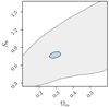 |
Fig. B.1. Prior range for the Ωm and S8 parameters compared to the 2σ contour from our fiducial cosmological analysis. |
Appendix C: Estimating the goodness of fit
To assess the goodness-of-fit of our model to the data it is necessary to determine the effective number of degrees of freedom, νeff, (see the discussion in Sect. 6.3 of Joachimi et al. 2021, on why νeff ≠ Ndata − Nθ, for a typical cosmology analysis with Ndata data points and Nθ cosmological parameters). We follow a simulation approach to determine νeff following Joachimi et al. (2021), Miyatake et al. (2022b).
We generate 200 noisy mock data vectors, drawing samples from the multivariate distribution defined by the mean, which is our best-fit signal, and the full covariance matrix. We find the maximum posterior point using a Nelder-Mead minimisation and its corresponding χ2 value for the fit. From the resulting distribution of χ2 values, shown in Fig. C.1, we fitted a χ2 distribution to find the effective degrees of freedom6, νeff = 147.55, finding that our model provides a good fit to the data with p(χ2|νeff) = 0.27.
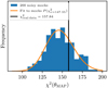 |
Fig. C.1. Estimation of the goodness of fit of the fiducial best-fit model at the MAP values. The histogram shows the distribution of the χ2 values from 200 noisy mock data vectors (see the main text for the detailed procedure). The orange line shows the fit of the χ2 distribution to the histogram, from which we obtain the effective number of degrees of freedom in the data. The vertical black line shows the χ2 value as obtained from the best-fit model to the real data. |
We can use our simulation approach to also determine the goodness of fit for each of the three sections of the data vector: ESD (galaxy-galaxy lensing), wp (galaxy clustering), and SMF. To estimate the degrees of freedom for each observable we find the χ2 value for that section of the data vector corresponding to the maximum posterior point that is found using the full data vector. In other words the partial χ2 values are not separately minimised. Fig. C.2 presents the resulting χ2 distributions and fit. We note that some alternative methods for defining νeff, such as that presented in Raveri & Hu (2019), would be ill defined for these sub-data vectors owing to the number of free parameters in the model, resulting in negative effective degree of freedom or negative effective number of parameters. We find  with
with ![Mathematical equation: $ p[\chi^2 ({\mathrm{ESD}}) | \nu^{\mathrm{ESD}}_{\mathrm{eff}}]=0.05 $](/articles/aa/full_html/2023/07/aa45158-22/aa45158-22-eq141.gif) ,
,  with
with ![Mathematical equation: $ p[\chi^2 ({w_{\mathrm{p}}}) | \nu^{w_{\mathrm{p}}}_{\mathrm{eff}}]=0.01 $](/articles/aa/full_html/2023/07/aa45158-22/aa45158-22-eq143.gif) , and
, and  with
with ![Mathematical equation: $ p[\chi^2 ({\mathrm{SMF}}) | \nu^{\mathrm{SMF}}_{\mathrm{eff}}]=0.39 $](/articles/aa/full_html/2023/07/aa45158-22/aa45158-22-eq145.gif) . We conclude that the goodness of fit of the full data vector and each of the individual sections is acceptable. This procedure is repeated for the remaining modelling cases considered in this paper.
. We conclude that the goodness of fit of the full data vector and each of the individual sections is acceptable. This procedure is repeated for the remaining modelling cases considered in this paper.
 |
Fig. C.2. Same as Fig. C.1, but for the three different observables in our analysis. The fits to the distributions are used to determine the number of degrees of freedom for each observable, which are in turn are used to determine the reduced χ2 values for each of them. Note that the χ2 distributions are not a result of maximising the posterior for that section of the mocks. The vertical lines show the χ2 values from the real data, matching in colours with the histograms. |
Appendix D: Galaxy-galaxy lensing random signal
The ratio between the lensing signal measured around random galaxies from the organised randoms catalogue and the fiducial model prediction in our six stellar mass bins is presented in Fig. D.1. A non-zero random signal indicates systematic effects in the ESD signal measured from the KiDS survey. The strong dependence of the random signal on the stellar mass of the lens bin indicates that this systematic is unlikely to be caused by residual uncorrected distortions in the source lensing catalogue, for example those associated with the point spread function of the camera. Such a data-related systematic would impact the ESD signal of each lens bin similarly given the similar source samples (see also Giblin et al. 2021, which presents a series of diagnostic tests). Instead we conclude that this signal arises from large-scale structure sample variance that differs as the volume of the sample grows with the increasing stellar mass (Singh et al. 2017). We calculate the error on the mean random signal, measured using 1000 samples of the random catalogue, finding it to be indistinguishable from the thickness of the blue curve, and sufficiently small that we do not include it in our overall error budget. We find that the random correction applied to the data exceeds 100% in the first three stellar mass bins on large scales, and can be up to 4 times larger than the statistical uncertainty.
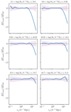 |
Fig. D.1. Ratio between the lensing signal measured around random galaxies from the organised randoms catalogue and the fiducial model prediction in our six stellar mass bins. For comparison, we show the uncertainty of the data as a purple band. |
Appendix E: Extensions to the fiducial cosmological analysis
In this appendix we review the impact of modelling choices on our fiducial cosmological parameter constraints (Sect. 4) to a series of extensions to our fiducial theoretical model. The results, in terms of S8 and Ωm are summarised in Fig. E.1 with the full parameter space quantified in Table E.1 and Fig. E.2.
 |
Fig. E.1. Comparison between S8 and Ωm values for our fiducial results and the tests for different modelling choices. All results are shown for maximum statistics of the marginal posterior distributions (MMAX) and corresponding credible interval. |
 |
Fig. E.2. Full posterior distributions of the model parameters (the priors are listed in Table 2). The contours indicate 1σ and 2σ confidence regions. |
Marginal constraints on all model parameters listed together with their priors, for the fiducial and extension setups considered.
E.1. Modelling intrinsic galaxy alignments and magnification
We quantified the contribution of lens galaxy magnification and intrinsic galaxy alignments to our data, which we do not account for in our fiducial model. We estimated the contribution of IAs using the NLA model (Bridle & King 2007) as
 (E.1)
(E.1)
where AIA is the amplitude of the IA signal, C1 is a normalisation constant, D(z) the linear growth factor. We set C1ρcrit = 0.0134, motivated by Brown et al. (2002). In order to estimate the contribution of IAs to the galaxy-galaxy lensing signal, we set AIA = 1, which is a good ‘worst-case’ scenario for our complete magnitude-limited KiDS-Bright sample. We project the PgI power spectrum to the galaxy-galaxy lensing signal. We subtract the additional contribution from the intrinsic alignments from the measured lensing signal and compare the relative difference between the corrected and uncorrected data to quantify the impact of neglecting intrinsic galaxy alignments in our theoretical model. Such a model only describes the IA well on large scales and becomes increasingly ad hoc on small scales, but it nevertheless provides a sensible amplitude estimation. Future studies will use the halo model based approach as presented in Fortuna et al. (2021) and Georgiou et al. (2019), which links the IA signal to the properties of the galaxies an their parent dark matter haloes.
The magnification contribution to the total lensing and clustering signal is modelled as
 (E.2)
(E.2)
and
 (E.3)
(E.3)
where ΔΣmm(rp) and wmm(rp) are the lensing signal and projected clustering contributions from the convergence power spectrum, respectively (Joachimi & Bridle 2010; Simon & Hilbert 2018; Unruh et al. 2020). The wgm(rp) is the same quantity as the Σ(rp), but without the mean density  (see Eq. 35). We estimate the contribution from lens magnification using the values for a KiDS and GAMA like survey, given by Unruh et al. (2020). We adopted αd = 0.85, which corresponds to a lens redshift of 0.21, and αd = 2.11 corresponding to a lens redshift of 0.36. These values are representative of the magnification effect we would expect for the two highest stellar mass bins in our analysis, with other bins predicted to have a somewhat smaller contribution, due to their redshifts (Unruh et al. 2020). We subtract the magnification contribution from our data to quantify the impact of neglecting magnification in our theoretical model.
The relative contributions of IAs and magnification to the ESD and wp observables are presented in Fig. E.3. We present the contribution for the largest stellar mass bin only, as the contribution to magnification and IAs is of the same order for all of them. In the same figure we also show the changes to the galaxy-galaxy lensing and galaxy clustering signals if we change the two main cosmological parameters. The contributions of both IAs and magnification are well below 1%, as also found in Unruh et al. (2020) and are well within the error budget of the data. Moreover, they are also subdominant to the changes due to the cosmological parameters of interest. Such contributions have negligible effects on the overall signal, and are unlikely to be a significant source of bias. To some extent the effects cancel each other out, as for the redshifts of our lens galaxies the magnification effect dilutes the signal, while the IAs add a similar contribution.
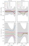 |
Fig. E.3. Relative difference between the lensing signal with and without the contribution of IAs and lens magnification. The IA contribution is modelled with AIA = 1, which is a reasonable ‘worst-case’ scenario for the KiDS-Bright sample, and the magnification is modelled with αd = 0.85 and αd = 2.11, typical for GAMA-like lenses at a redshift of 0.21 and 0.36. Grey areas show the error on the data. We also show the changes to the galaxy-galaxy lensing and galaxy clustering signals if we change the two main cosmological parameters. The behaviour is only shown for the largest stellar mass bin, as the contribution to magnification and IAs is of the same order for all of them. |
E.2. Changing the ns prior
Inspecting Fig. E.2, we note that the marginalised posteriors of our prior-informed cosmological parameter set, ns, Ωb and h, have a tendency to push up against one side of the prior. As the KiDS 2 × 2 pt+SMF data vector is expected to be insensitive to changes in this parameter set, we conclude that this effect arises from projection effects or the MCMC not fully sampling this part of parameter space. Given that there are no strong degeneracies between this set and the rest of the parameters, and that the set is already well constrained from other studies (see the discussion in Appendix B of Heymans et al. 2021) we find no motivation to investigate the impact of widening the priors. Instead we investigated reducing the prior range by adopting a Gaussian prior with the mean and uncertainty fixed to the Planck Collaboration VI (2020) constraint for ns. This parameter is the most interesting to investigate of the three, as any tension between small and large scales may be expected to manifest in a biased spectral index constraint (Tröster et al. 2021).
The results are presented in Table E.1 and Fig. E.2. We find that the marginal contours for the parameters do not change significantly with the addition of a restrictive prior on ns. For example, the MMAX estimate of S8, shifts by 0.13σ, which is consistent with the expected MCMC run-to-run variance (Joachimi et al. 2021). In future studies, we will explore the impact of using more restrictive priors on all the externally constrained parameters that we are insensitive to, noting that this may also help reduce projection bias for posteriors with many parameters.
E.3. The effect of un-modelled photometric redshift errors on the projected galaxy clustering measurements
In Sect. 3.3 we introduce a free nuisance parameter, 𝒟 (Eq. 43), to account for our uncertainty on the amplitude of the true projected galaxy clustering signal. The expected dilution is a result of unaccounted photometric redshift errors in our theoretical model for wp(rp). In Fig. E.4 we compare our fiducial constraints in S8 and Ωm with the constraints from an analysis where the photometric redshift dilution effect is neglected and 𝒟 = 1. We find that while the omittance of the photometric redshift dilution effect does not impact the S8 constraints, Ωm becomes biased and more constrained. This is expected as the galaxy clustering is more sensitive to Ωm compared to σ8 (cf. Fig. E.3). This motivates future work to improve the estimator for, or theoretical modelling of, the projected galaxy clustering signal in the presence of photometric redshift errors, following Joachimi et al. (2011), Chisari et al. (2014).
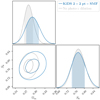 |
Fig. E.4. Marginalised constraints for the joint distributions of S8 and Ωm, showing the 68% and 95% credible regions. We compare our fiducial analysis (blue) with an analysis that neglects the impact of photometric redshift uncertainties, which dilute the estimated projected galaxy clustering signal (grey). |
All Tables
KiDS-Bright stellar mass samples: overview of the number of lens galaxies, median stellar masses, M⋆, med, and median redshifts, zmed.
Marginal constraints on all model parameters, listed together with their priors.
Marginal constraints on all model parameters listed together with their priors, for the fiducial and extension setups considered.
All Figures
|
Fig. 1. Galaxy stellar mass as a function of ANNz2 photometric redshift for the KiDS-Bright sample. The full sample is shown with a logarithmic hexagonal density plot. The blue line shows the stellar mass limit determined using the automated method presented by Wright et al. (2017). Red boxes show the six stellar mass bins used in the analysis, with individual galaxies plotted as black dots. The bin ranges were chosen in such a way as to achieve a good signal-to-noise ratio in all bins for our galaxy-galaxy lensing and galaxy clustering measurements. |
| In the text | |
|
Fig. 2. KiDS-Bright galaxy SMF and the fractional errors. Upper panel: KiDS-Bright galaxy SMF (crosses) compared to the model from Wright et al. (2018), evaluated at the median redshift of our sample (black dashed line). The blue line and shaded region indicates the best-fit model and 68% confidence levels of our best-fit halo model (Eq. (22)). We caution that the quality of the fit cannot be judged by eye, because of the covariance in the data, between the data points and between the other observables. The reduced χ2 value for this observable is 1.05 (d.o.f. = 14.58, p-value = 0.39), estimated using the method presented in Appendix C. Lower panel: Fractional errors on the data and the model, ΔΦ/δΦ. |
| In the text | |
|
Fig. 3. Galaxy-galaxy lensing: the stacked ESD profiles of the six stellar mass bins in the KiDS-Bright galaxy sample defined in Table 1. The solid lines represent the best fitting fiducial ESD halo model (Sect. 2.3, Eq. (34)) as obtained using an MCMC fit, with the 68 percent confidence interval indicated with a shaded region. We caution that the quality of the fit cannot be judged by eye, because of the covariance in the data between the observed bins and also between the observables. The reduced χ2 value for this observable is 1.28 (d.o.f. = 73.18, p-value = 0.05), estimated using the method presented in Appendix C. |
| In the text | |
|
Fig. 4. Galaxy clustering: the projected galaxy clustering signal of the six stellar mass bins in the KiDS-Bright galaxy sample defined in Table 1. The solid lines represent the best fitting fiducial halo model (Sect. 2.3, Eq. (27)) as obtained using an MCMC fit, with the 68 percent confidence interval indicated with a shaded region. We caution that the quality of the fit cannot be judged by eye, because of the covariance in the data, between the observed bins and between the observables. The reduced χ2 value for this observable is 1.42 (d.o.f. = 71.62, p-value = 0.01), estimated using the method presented in Appendix C. |
| In the text | |
|
Fig. 5. Marginalised constraints for the joint distributions of S8 and Ωm. The 68% and 95% credible regions for the 2 × 2 pt+SMF fiducial analysis (blue) can be compared with constraints from KiDS cosmic shear (Asgari et al. 2021b, pink), KiDS with BOSS 3 × 2 pt (Heymans et al. 2021, purple), and the CMB Planck Collaboration VI (2020, black). |
| In the text | |
|
Fig. 6. Joint-probe comparison of S8 and Ωm constraints. Our fiducial results (KiDS 2 × 2 pt +SMF) can be compared to: a similar 2 × 2 pt +SMF analysis from the SDSS (Cacciato et al. 2013); a series of 2 × 2 pt studies that includes the latest results from DES (Porredon et al. 2022; Pandey et al. 2022) and the HSC survey (Miyatake et al. 2022b); and 3 × 2 pt analyses from KiDS with BOSS (Heymans et al. 2021) and DES (DES Collaboration 2022). The last entry shows the Planck Collaboration VI (2020, TT,TE,EE+lowE) constraints. Our results are consistent with all studies, including Planck Collaboration VI (2020), although we find a mild tension between our S8 constraints and those from Planck, at the level of 1.9σ. |
| In the text | |
|
Fig. 7. Stellar-to-halo mass relation, as defined by Eq. (19), using the best-fit HOD parameters from our 2 × 2 pt+SMF analysis (blue). The result can be compared to results from Leauthaud et al. (2012, green), Moster et al. (2013, black), Coupon et al. (2015, orange), and van Uitert et al. (2016, purple). The grey area shows the range in stellar masses where the obtained stellar-to-halo mass relation is extrapolated beyond the range of median stellar masses used in this analysis. |
| In the text | |
|
Fig. 8. Poissonian parameter, 𝒫 (Eq. (52)), as a function of dynamical group mass, Mdyn, for GAMA galaxy groups with three or more members (blue), and groups with five or more members (white). The orange and green lines show the best-fit power law (Eq. (53)) to the GAMA/2 × 2 pt+SMF data, with the green-shaded region showing the uncertainty on the 2 × 2 pt+SMF fit. The fiducial, single value model for 𝒫 is shown with the grey horizontal band. With the wiggly grey-shaded areas, we show the approximate range of dynamical group masses that are outside the halo mass range of our analysis. |
| In the text | |
|
Fig. B.1. Prior range for the Ωm and S8 parameters compared to the 2σ contour from our fiducial cosmological analysis. |
| In the text | |
|
Fig. C.1. Estimation of the goodness of fit of the fiducial best-fit model at the MAP values. The histogram shows the distribution of the χ2 values from 200 noisy mock data vectors (see the main text for the detailed procedure). The orange line shows the fit of the χ2 distribution to the histogram, from which we obtain the effective number of degrees of freedom in the data. The vertical black line shows the χ2 value as obtained from the best-fit model to the real data. |
| In the text | |
|
Fig. C.2. Same as Fig. C.1, but for the three different observables in our analysis. The fits to the distributions are used to determine the number of degrees of freedom for each observable, which are in turn are used to determine the reduced χ2 values for each of them. Note that the χ2 distributions are not a result of maximising the posterior for that section of the mocks. The vertical lines show the χ2 values from the real data, matching in colours with the histograms. |
| In the text | |
|
Fig. D.1. Ratio between the lensing signal measured around random galaxies from the organised randoms catalogue and the fiducial model prediction in our six stellar mass bins. For comparison, we show the uncertainty of the data as a purple band. |
| In the text | |
|
Fig. E.1. Comparison between S8 and Ωm values for our fiducial results and the tests for different modelling choices. All results are shown for maximum statistics of the marginal posterior distributions (MMAX) and corresponding credible interval. |
| In the text | |
|
Fig. E.2. Full posterior distributions of the model parameters (the priors are listed in Table 2). The contours indicate 1σ and 2σ confidence regions. |
| In the text | |
|
Fig. E.3. Relative difference between the lensing signal with and without the contribution of IAs and lens magnification. The IA contribution is modelled with AIA = 1, which is a reasonable ‘worst-case’ scenario for the KiDS-Bright sample, and the magnification is modelled with αd = 0.85 and αd = 2.11, typical for GAMA-like lenses at a redshift of 0.21 and 0.36. Grey areas show the error on the data. We also show the changes to the galaxy-galaxy lensing and galaxy clustering signals if we change the two main cosmological parameters. The behaviour is only shown for the largest stellar mass bin, as the contribution to magnification and IAs is of the same order for all of them. |
| In the text | |
|
Fig. E.4. Marginalised constraints for the joint distributions of S8 and Ωm, showing the 68% and 95% credible regions. We compare our fiducial analysis (blue) with an analysis that neglects the impact of photometric redshift uncertainties, which dilute the estimated projected galaxy clustering signal (grey). |
| In the text | |
Current usage metrics show cumulative count of Article Views (full-text article views including HTML views, PDF and ePub downloads, according to the available data) and Abstracts Views on Vision4Press platform.
Data correspond to usage on the plateform after 2015. The current usage metrics is available 48-96 hours after online publication and is updated daily on week days.
Initial download of the metrics may take a while.