| Issue |
A&A
Volume 699, July 2025
|
|
|---|---|---|
| Article Number | A124 | |
| Number of page(s) | 38 | |
| Section | Cosmology (including clusters of galaxies) | |
| DOI | https://doi.org/10.1051/0004-6361/202452592 | |
| Published online | 07 July 2025 | |
KiDS-Legacy: Covariance validation and the unified OneCovariance framework for projected large-scale structure observables
1
Argelander-Institut für Astronomie, Universität Bonn, Auf dem Hügel 71, D-53121 Bonn, Germany
2
Ruhr University Bochum, Faculty of Physics and Astronomy, Astronomical Institute (AIRUB), German Centre for Cosmological Lensing, 44780 Bochum, Germany
3
School of Mathematics, Statistics and Physics, Newcastle University, Herschel Building, NE1 7RU, Newcastle-upon-Tyne, UK
4
Department of Physics and Astronomy, University College London, Gower Street, London WC1E 6BT, UK
5
Department of Physics, Institute for Computational Cosmology, Durham University, South Road, Durham DH1 3LE, UK
6
Department of Physics, Centre for Extragalactic Astronomy, Durham University, South Road, Durham DH1 3LE, UK
7
E. A. Milne Centre, University of Hull, Cottingham Road, Hull, HU6 7RX, UK
8
Centre of Excellence for Data Science, AI, and Modelling (DAIM), University of Hull, Cottingham Road, Hull, HU6 7RX, UK
9
Center for Theoretical Physics, Polish Academy of Sciences, al. Lotników 32/46, 02-668 Warsaw, Poland
10
Department of Physics and Astronomy, University of Waterloo, 200 University Ave W, Waterloo, ON N2L 3G1, Canada
11
Institute for Theoretical Physics, Utrecht University, Princetonplein 5, 3584CC Utrecht, The Netherlands
12
Institute for Astronomy, University of Edinburgh, Blackford Hill, Edinburgh, EH9 3HJ, UK
13
Centro de Investigaciones Energéticas, Medioambientales y Tecnológicas (CIEMAT), Av. Complutense 40, E-28040 Madrid, Spain
14
Institute of Cosmology & Gravitation, Dennis Sciama Building, University of Portsmouth, Portsmouth, PO1 3FX, United Kingdom
15
Leiden Observatory, Leiden University, PO Box 9513, 2300 RA Leiden, The Netherlands
16
Aix-Marseille Université, CNRS, CNES, LAM, Marseille, France
17
Universität Innsbruck, Institut für Astro- und Teilchenphysik, Technikerstr. 25/8, 6020 Innsbruck, Austria
18
Donostia International Physics Center, Manuel Lardizabal Ibilbidea, 4, 20018 Donostia, Gipuzkoa, Spain
19
INAF – Osservatorio Astronomico di Roma, Via Frascati 33, 00040 Monteporzio Catone (Roma), Italy
20
INFN – Sezione di Roma, Piazzale Aldo Moro, 2 – c/o Dipartimento di Fisica, Edificio G. Marconi, I-00185 Roma, Italy
21
Institute for Particle Physics and Astrophysics, ETH Zürich Wolfgang-Pauli-Strasse 27, 8093 Zürich, Switzerland
⋆ Corresponding author: This email address is being protected from spambots. You need JavaScript enabled to view it.
, This email address is being protected from spambots. You need JavaScript enabled to view it.
Received:
12
October
2024
Accepted:
16
March
2025
Abstract
We introduce OneCovariance, an open-source software designed to accurately compute covariance matrices for an arbitrary set of two-point summary statistics across a variety of large-scale structure tracers. Utilising the halo model, we estimated the statistical properties of matter and biased tracer fields, incorporating all Gaussian, non-Gaussian, and super-sample covariance terms. The flexible configuration permits user-specific parameters, such as the complexity of survey geometry, the halo occupation distribution employed to define each galaxy sample, or the form of the real-space and/or Fourier space statistics to be analysed. We illustrate the capabilities of OneCovariance within the context of a cosmic shear analysis of the final data release of the Kilo-Degree Survey (KiDS-Legacy). Upon comparing our estimated covariance with measurements from mock data and calculations from independent software, we ascertain that OneCovariance achieves accuracy at the per cent level. When assessing the impact of ignoring complex survey geometry in the cosmic shear covariance computation, we discover misestimations at approximately the 10% level for cosmic variance terms. Nonetheless, these discrepancies do not significantly affect the KiDS-Legacy recovery of cosmological parameters. We derive the cross-covariance between real-space correlation functions, bandpowers, and COSEBIs, facilitating future consistency tests among these three cosmic shear statistics. Additionally, we calculate the covariance matrix of photometric-spectroscopic galaxy clustering measurements, validating the jackknife covariance estimates for calibrating KiDS-Legacy redshift distributions. The OneCovariance can be found on GitHub (https://github.com/rreischke/OneCovariance) together with comprehensive documentation and examples.
Key words: cosmological parameters / cosmology: observations / cosmology: theory / large-scale structure of Universe
© The Authors 2025
 Open Access article, published by EDP Sciences, under the terms of the Creative Commons Attribution License (https://creativecommons.org/licenses/by/4.0), which permits unrestricted use, distribution, and reproduction in any medium, provided the original work is properly cited.
This article is published in open access under the Subscribe to Open model. This email address is being protected from spambots. You need JavaScript enabled to view it. to support open access publication.
1. Introduction
The current best practice for testing the cosmological model of the Universe using the large-scale structure (LSS) are two-point functions. These measurements typically involve the coherent weak lensing distortion of galaxy images and the correlation of galaxy positions. All of them have been successfully measured and used for cosmological inference by the Kilo-Degree Survey (KiDS, see e.g. Hildebrandt et al. 2017; Asgari et al. 2021b; Heymans et al. 2021)1, the Dark Energy Survey (DES, see e.g. Abbott et al. 2018, 2022; Amon et al. 2022)2, and the Subaru Hyper Suprime-Cam (HSC, see e.g. Sugiyama et al. 2022; Hamana et al. 2020; Dalal et al. 2023)3. These experiments have laid the groundwork for upcoming stage 4 surveys such as Euclid4, The Legacy Survey of Space and Time (LSST)5, and Roman6. Leveraging galaxy positions and shapes enables the measurement of three unique two-point functions, shape-shape (cosmic shear, CS), shape-position (galaxy-galaxy-lensing, GGL), and position-position (galaxy clustering, GC). Aggregating these into a data vector establishes the standard 3×2-point analysis. The main ingredient in this kind of analysis is the likelihood, which is commonly assumed to be Gaussian, so that it can be completely characterised by the data vector, model prediction, and covariance.
There are various approaches to computing or estimating the covariance matrix. The most direct method involves utilising the data itself, generating pseudo-realisations through subsampling (Norberg et al. 2009; Friedrich et al. 2016; Mohammad & Percival 2022; Trusov et al. 2024). Alternatively, simulation suites can be used to estimate the covariance if enough realisations are available and feasible (Hartlap et al. 2007; Harnois-Déraps et al. 2012, 2018; Dodelson & Schneider 2013; Heymans et al. 2013; Taylor et al. 2013; Taylor & Joachimi 2014; Joachimi 2017; Sellentin & Heavens 2018). Lastly, theoretical modelling is usually the most efficient and arguably the most fundamental way to estimate the covariance matrix (Takada & Jain 2004; Eifler et al. 2009; Krause & Eifler 2017; Reischke et al. 2017; Joachimi et al. 2021; Friedrich et al. 2021). Each approach has its own advantages and disadvantages. Simulations tend to be relatively accurate, with systematic effects such as masking or variable survey depth easily accounted for. However, obtaining an unbiased covariance estimate necessitates numerous realisations, with at least as many simulations required as there are effective degrees of freedom in the data for the covariance matrix to be invertible. Current surveys typically involve around 102−103 data points, while upcoming stage 4 surveys will boast 104 data points for standard two-point statistics. Consequently, significant data compression (e.g. Heavens et al. 2000, 2017; Asgari & Schneider 2015) or running numerous computationally intensive simulations is necessary. Conversely, theoretical covariances are comparatively inexpensive to compute, although modelling the aforementioned systematic effects is difficult and a simulation-based covariance matrix estimation might be more accurate. While subsampling techniques offer a potential quick way to self-consistently estimate the covariance directly from the data, they tend to be biased on large scales where the subsamples are not independent due to cosmic variance.
Due to the symmetries of the Friedmann-Lemaître-Robertson-Walker metric, theoretical computations are typically conducted in harmonic (Fourier) space. Rotational symmetry results in the decoupling of different angular multipoles, ℓ, and allow considerable data compression. However, observations of a masked sky compromise the orthogonality of the spherical harmonic basis, leading to mode coupling that necessitates careful modelling, known as pseudo-Cℓ (see e.g. Hikage et al. 2011, 2019; Becker et al. 2016; Alonso et al. 2019; Nicola et al. 2021; Loureiro et al. 2022; von Wietersheim-Kramsta et al. 2025). Unlike in harmonic space, standard real space correlation functions do not face these limitations to the first order in signal modelling, they encompass w(θ), γt(θ), and ξ±(θ) for GC, GGL, and CS respectively7 However, photometric galaxy surveys introduce a broad radial window function, mixing different physical scales and complicating efforts to disentangle them and mitigate astrophysical effects on small scales. Moreover, correlation functions integrate over the angular power spectra with an oscillatory but broad integration kernel, resulting in limited control over the physical scales influencing the measurements. Leakage from very low multipoles can alter the Gaussianity of the likelihood at large angular scales (Sellentin et al. 2018; Louca & Sellentin 2020; Oehl & Tröster 2024), while significant contributions from highly non-linear and theoretically uncertain scales occur at small angular separations. Importantly, the cosmological lensing signal does not produce B-modes to first order, as it represents the gradient of the lensing potential. Consequently, the B-mode signal serves as a consistency check for systematic effects. However, real space correlation functions mix E- and B-modes, complicating the interpretation of these tests (see e.g. Schneider & Kilbinger 2007).
The aforementioned problems of real space correlation functions are partially alleviated by considering different derived summary statistics. In weak lensing surveys and in particular KiDS, two alternatives to real space correlation functions used are band powers (Schneider et al. 2002) and COSEBIs (Schneider et al. 2010). While the former approximately separates E and B modes, the latter yields a complete separation by definition. The demonstration of consistent parameter constraints over a set of summary statistics adds significant confirmation to the robustness of the pipelines used, the systematics involved and the overall fidelity of the cosmological inference. Although many of these methods have been integrated within the community for a 3×2-point analysis and are publicly available for model predictions, a unified framework for the covariance matrix in the cosmological community for all kinds of summary statistics has been absent.
While some of the previously mentioned tools for calculating the covariance matrix are publicly available (see e.g. Krause & Eifler 2017; Fang et al. 2020), they possess limited flexibility or lack comprehensive functionality when it comes to exchanging tracer fields, summary statistics, weight functions, bias, or halo occupation distribution prescriptions. Furthermore, it is not always straightforward to input files of pre-calculated quantities into these codes. Therefore, this paper presents the analytical covariance matrices alongside a Python code, the OneCovariance code, encompassing all functionalities used in the standard analysis of KiDS, ranging from CS (Asgari et al. 2021b) alone to a full 3×2-point analysis (Joachimi et al. 2021; Heymans et al. 2021), incorporating the stellar mass function (Dvornik et al. 2023), and employing all three types of summary statistics (i.e. real space correlation functions, bandpowers, and COSEBIs/Ψ-stats8) used in KiDS for CS, galaxy clustering, and galaxy–galaxy lensing as well as arbitrary cross-correlations between them. Moreover, it remains flexible enough to accommodate very general inputs and therefore can be used by any survey or collaboration to obtain quick and easy covariance matrices for photometric LSS observables.
The goal of this paper is threefold: (i) to furnish a comprehensive and instructive document encompassing all components required for theoretical computations of LSS covariances in photometric galaxy surveys, consolidating everything into a unified code, which we call OneCovariance, accessible to the cosmological community for generating covariance matrices effortlessly for any projected LSS parameter; (ii) to introduce the mocks used for the validation of the covariance matrix in the final CS analysis of the Kilo-Degree Survey (KiDS-Legacy) featuring, among other things, a realistic footprint and variable number density; and (iii) to employ the OneCovariance code in different scenarios. Our focus here, in addition to CS in KiDS-Legacy, includes the covariance matrix of clustering redshifts (van den Busch et al. 2020) and the cross-correlation between different summary statistics (Asgari et al. 2021b). It should be highlighted that the OneCovariance code, while showcased for KiDS, is completely general and can be used for all different types of analyses via simple file inputs to acquire fast covariance estimates.
Since the CS catalogue of KiDS-Legacy is not final at this stage, we only performed simulations and comparisons for KiDS-Legacy-like settings. However, we do not anticipate any major changes that would influence the covariance validation. We refer to data products that are final as of the writing of this paper as KiDS-Legacy, and to simulations or data products with nearly final settings as KiDS-Legacy-like. Furthermore, we generally refer to KiDS-Legacy as the entirety of the final analysis of the last data release of KiDS.
The manuscript is organised as follows. In Section 2 we discuss some general properties of covariance matrices in cosmology, its definition, the different contributions, and the flat sky approximation. In Section 3 we discuss the prescription for non-linear structure formation. Here we focus on a halo model-based description of structure formation, and we discuss all its ingredients. The projection along the line of sight and the corresponding covariance in harmonic space is discussed in Section 4. We then discuss the projection to observables in Section 5 and describe the motivation and features of the OneCovariance code in Section 6. The subsequent sections feature applications of the code to specific examples. We introduce a KiDS-Legacy-like CS sample in Section 7 and describe the general characteristics of the covariance matrix as well as the influence of its modelling choices on parameter inference. Then, in Section 8 we present the KiDS-Legacy-like mocks, incorporating variable depth, and we demonstrate the overall agreement between the analytical and numerical covariances. The results section concludes with Section 9, which showcases two additional applications of the covariance matrix utilised in KiDS-Legacy: covariances between different summary statistics for consistency tests and the covariance for clustering redshift calibration. To facilitate swift access, we highlight key plots at the outset of each results section. Finally, in Section 10 and Section 11 we examine the current status and capabilities of the code, along with future directions and our conclusions.
2. Covariance matrices in photometric galaxy surveys
In this section, we outline the general theoretical modelling involved in constructing the covariance matrix. We separate this discussion from the precise prescription of non-linear structure formation, which is described in more detail in Section 3. This separation allows us to distinguish observational definitions from the theoretical framework as clearly as possible.
2.1. General considerations
Cosmological analyses of the LSS hinge on estimating a two-point function between any pair of observables (tracers), denoted as ti[δ], which are functionals of the underlying matter field, δ(x,χ). Here, x represents a spatial co-moving vector (i.e. a 3-dimensional vector in a spatial hyper-surface), and χ denotes the co-moving distance. These two-point functions can be aggregated into a vector  with components
![Mathematical equation: $$ {\cal {{O}}}_\alpha {{\scriptstyle:\!\!}=} \left \langle t_i[\delta ] t_j[\delta ]\right \rangle \; \quad \alpha \in {\{ }{\textrm {all unique combinations of ${(t_i,t_j)}$}}{\} }\,. $$](/articles/aa/full_html/2025/07/aa52592-24/aa52592-24-eq2.gif) (1)
(1)
Here, the angular brackets, 〈·〉, denote an ensemble average, akin to a spatial average (for more details on this ergodicity argument see e.g. Desjacques et al. 2021). The number of unique combinations depends on the tracer used; if the underlying tracer is the same and i simply labels a subset such as tomographic bins, i≤j, otherwise, all combinations can exist. The components of the covariance matrix are then defined as
 (2)
(2)
Typically, we are provided with the statistical properties of the density field δ from theoretical calculations or numerical simulations, rather than those of its tracer. If the mapping from δ to ti is linear, all the statistical properties of δ extend accordingly to ti. However, this is not always the case, such as in a perturbative bias expansion or the reduced shear beyond linear order. For simplicity, we assume 〈ti[δ]〉=0, resulting in the following breakdown of Equation (2) using Equation (1) and Wick's theorem:
 (3)
(3)
Here, we have omitted the argument of the different tracers, [δ], for notational simplicity. The first two terms are known as Gaussian terms, deriving from products of the original observable, while the subscript ‘c’ in the last term denotes the connected part of the correlator, i.e. the term originating from a genuine four-point function and not the product of two-point function. This quantity vanishes for Gaussian fields. For surveys with incomplete sky coverage, the connected part of the covariance can be decomposed into a part arising from modes within the survey, termed the non-Gaussian (nG) component, and a term generated by modes larger than the survey, known as the super-sample covariance (SSC, Takada & Hu 2013):
 (4)
(4)
It should be noted that both these terms are entirely arising from the connected term. Particularly, the SSC term stems from the cosmic variance's reaction to unobservable modes, manifested as the squeezed limit of a connected four-point function (Linke et al. 2024).
Real observables invariably serve as discrete tracers of the underlying smooth field, hence they are subject to stochastic noise due to the finite number of tracers, such as galaxies. Hence, one can schematically express
 (5)
(5)
where ni denotes some stochastic noise component, this component emerges only when the same object correlates with itself and is thus also referred to as the shot or shape noise component for galaxy clustering or CS, respectively. With this understanding, assuming that the signal does not correlate with the noise, the Gaussian terms, i.e., the first two terms in Equation (3), each decompose into three components,
 (6)
(6)
that are distinguished by their scaling with the signal. We note that the sample variance term is often called cosmic variance in the literature.
2.2. Angular polyspectra and Limber approximation
Observables of (photometric) galaxy surveys are projected quantities of three-dimensional fields. Consider such a three-dimensional field A(x,fKχ(z))∈{ti} at position x and redshift z. Its projected version,  , is
, is
 (7)
(7)
where WA(χ) is some weighting function whose exact form is probe specific and will be discussed in Section 4.  is the unit vector on the sphere and fK(χ) is the co-moving angular diameter distance, such that
  and χ the co-moving radial distance. In Appendix B the definitions for a spherical harmonic decomposition of the projected field, a, are given. Leveraging those relations, the two-point function defines the angular power spectrum,
  , of the two-dimensional fields a1 and a2 as follows:
 (8)
(8)
Here the dependence on χ1 and χ2 of the three-dimensional power spectrum,  , was made explicit.
  is the Kronecker delta. The more general equation for higher-order correlators is provided in Appendix C. Throughout this paper the geometric mean is used to approximate the unequal time correlator such that for the power spectrum
![Mathematical equation: $$ P_{A_1A_2}(k, \chi _1,\chi _2) \approx \left [P_{A_1A_2}(k, \chi _1)P_{A_1A_2}(k, \chi _2)\right ]^{1/2}\,, $$](/articles/aa/full_html/2025/07/aa52592-24/aa52592-24-eq16.gif) (9)
(9)
which is an excellent approximation for almost all practical purposes (Castro et al. 2005; Kitching & Heavens 2017; Kilbinger et al. 2017; Chisari & Pontzen 2019; de la Bella et al. 2021).
In the flat sky limit (in which case the transform to spherical harmonics essentially becomes a two-dimensional Fourier transform, see Appendix D) angular polyspectra can be approximated using the Limber approximation (Limber 1953; Loverde & Afshordi 2008; Leonard et al. 2023):
 (10)
(10)
Here geometrical factors occurring in Equation (C.7) are disregarded due to the flat sky approximation. For n>3 this expression assumes that the angular average over possible configurations has already been carried out on the flat sky. The use of the Limber approximation introduces negligible biases in cosmological parameter inference when considering CS only (ss e.g. Joachimi et al. 2021; Leonard et al. 2023). Therefore, unless stated otherwise, we utilise Equation (10) for projected fields.
3. Non-linear evolution: Halo model
Due to the non-linearity of gravity and the complex interaction between cold dark matter and baryons, understanding structure formation in cosmology presents a formidable challenge. Various approaches have been developed to tackle this issue. These include standard perturbation theory (SPT, for an exhaustive review see Bernardeau et al. 2002), halo model approaches (HM, see e.g. Seljak 2000; Cooray & Sheth 2002; Asgari et al. 2023), effective field theory (EFT, Carrasco et al. 2012), or kinetic field theory (KFT, e.g. Bartelmann et al. 2021).
In addition to modelling the non-linear evolution of the smooth dark matter density field, there are additional complications: (i) The total matter power spectrum encapsulates the clustering of both cold dark matter and baryons. Processes such as star formation, supernovae, active galactic nuclei (AGN), and cooling can displace baryons relative to dark matter, leading to a spatial distribution of total matter that differs from that of cold dark matter alone. This phenomenon is collectively known as baryonic feedback (see e.g. Semboloni et al. 2013; Somerville & Davé 2015; Vogelsberger et al. 2020; Chisari et al. 2019b; Nicola et al. 2022). (ii) The tracers discussed in Section 2 are biased representations of the underlying matter distribution. This bias is most prominent in galaxy surveys (referred to as galaxy bias, see e.g. Desjacques et al. 2018, for a review), but also affects CS measurements through intrinsic alignment (IA) effects (see e.g. Schaefer 2009; Joachimi et al. 2015; Vlah et al. 2020; Fortuna et al. 2020, for reviews), which can be treated similarly to galaxy bias using an effective field theory (EFT) approach.
While perturbative approaches such as EFT are technically more rigorous than non-perturbative (but phenomenological) halo model calculations, they do not allow progressing into the highly non-linear regime, which is crucial for signals with low signal-to-noise ratios such as CS. In other words, the significance of the CS measurement is not large enough to fit all the EFT nuisance parameters and all cosmological information would be lost. Hence, incorporating prior knowledge regarding the statistical properties of the matter distribution via a halo model is key if one wants to access highly non-linear scales. Although KFT offers, in theory, an alternative route, it still has to be shown to provide good fits for models including baryonic feedback and higher-order statistics necessary for the covariance. Since the halo model has been shown to be flexible enough to describe different cosmological observations into the non-linear regime9 (see Mead et al. 2020, and references therein), we stick to a halo model approach in this paper, following the methodology of KiDS-1000 (Joachimi et al. 2021). However, it is worth noting that the code presented here is sufficiently flexible to accommodate any external power spectra, power spectrum response, and/or tri-spectra for subsequent calculations. The halo model assumes that the cosmic density field is entirely composed of dark matter halos, whose distribution is governed by a mass function. By assuming a density profile and a halo bias, we can calculate the statistical properties of the matter field. Populating each halo with galaxies using a halo occupation distribution (HOD) enables a versatile model that accurately predicts the statistical properties of CS, GC, GGL for the cross-correlation between the two galaxy samples.
3.1. Halo model ingredients: Galaxy bias and halo occupation distribution
Here, we briefly summarise the components involved in the halo model calculations of matter and galaxy polyspectra. Galaxy bias is addressed through an HOD prescription (van den Bosch et al. 2013; Dvornik et al. 2018, 2023; Lacasa et al. 2014; Lacasa 2018; Reischke et al. 2020). To achieve this, one employs a biasing function, b(M), depending on halo mass M, defined via the average number density of galaxies 〈N|M〉 in a halo of mass M
 (11)
(11)
where  is the average number density of galaxies and
  is the mean matter density in the Universe at redshift z. Average quantities in the occupation distribution are defined as
 (12)
(12)
where P(N|M) is the probability of a halo to be occupied with N galaxies. Moments of the bias at a redshift z, or any halo-related quantity, A(M,z), are calculated via the differential number density of halos of mass M: the halo mass function nh(M,z)
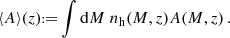 (13)
(13)
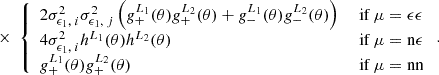
The halo model assumes that all matter in the Universe is bound in halos. We assume those halos to be spherically symmetric and to have an average density profile ρh(r|M)=Muh(r|M), such that uh is normalised and can be used in Equation (13) without introducing additional normalisation factors. The galaxy populations can be split into central, ‘c’, and satellite, ‘s’, galaxies with different halo profiles uc/s and halo occupations 〈Nc/s|M〉. If there is a central galaxy in a halo on average, 〈Nc|M〉=1 the distribution of additional galaxies, i.e. the satellites, is assumed to be Poisonnian. This allows us to calculate the expected number of n-tuples, 〈N(n)|M〉 in a halo, as required for the 1, …, 4-halo terms
 (14)
(14)
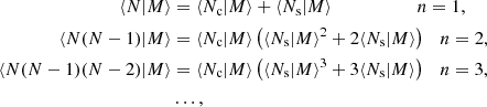
where the number of tuples for each individual type e.g. ‘s’ and ‘c’ can be read off. In the case of matter, ‘m’, the HOD is set to the halo mass M for each point and the normalisation is taken care of by  , i.e. 〈Nm|M〉=M. It should be noted that sub-Poissonian behaviour was found in Dvornik et al. (2023) for the satellite population. This could, in principle, be accounted for by including an additional free parameter on the two-point level. For the connected non-Gaussian term, this might lead to more complications. However, we do not expect that the latter is dominating and would change cosmological results significantly. It is instructive to introduce the following integrals (Cooray & Hu 2001; Takada & Hu 2013; Lacasa 2018) for the species X1,…,Xμ:
 (15)
(15)
Here  is the halo bias, for which we use the fitting function from Tinker & Wetzel (2010).
  is the Fourier transform of the normalised halo profile. In Appendix E we provide
  for an NFW profile. However, they are in general arbitrary. Lastly, the average number density nX(z) can be calculated using Equation (13):
 (16)
(16)
We note again that  with this definition.
3.2. Conditional stellar mass function
It remains to specify the occupation statistics of a galaxy with halo mass M. As the fiducial model, we chose the conditional stellar mass function (CSMF, Yang et al. 2009; Cacciato et al. 2009, 2013; van Uitert et al. 2016; Dvornik et al. 2018, 2023), specifying the average distribution of galaxies of stellar mass M★ given they occupy a halo with mass M. It is also split into centrals and satellites so that the total CSMF is
 (17)
(17)
The two contributions are modelled as a log-normal and a modified Schechter function
![Mathematical equation: $$ \begin{aligned}\Phi _\mathrm {c}(M_\star |M) &= \frac {1}{\sqrt {2\uppi }\ln (10)\sigma _\mathrm {c}M_\star }\exp \left [-\frac {\log (M_\star /M^*_\mathrm {c})^2}{2\sigma ^2_\mathrm {c}}\right ],\\ \Phi _\mathrm {s}(M_\star |M) &= \frac {\phi ^*_\mathrm {s}}{M^*_\mathrm {s}}\left (\frac {M_\star }{M^*_\mathrm {s}}\right )^{\alpha _\mathrm {s}}\exp \left [-\left (\frac {M_\star }{M^*_\mathrm {s}}\right )^2\right ], \end{aligned} $$](/articles/aa/full_html/2025/07/aa52592-24/aa52592-24-eq32.gif) (18)
(18)
for centrals and satellites respectively10. Here σc describes the scatter of stellar mass given a halo mass while αs describes the power law scaling of the satellite abundance. It should be noticed that if αs<0 the expression for Φs(M★|M) would formally diverge for low masses. However, the existence of satellites in the HOD are always conditioned on the existence of a central galaxy, thus ensuring convergence at low masses due to the exponential cut-off of Φc(M★|M). All free parameters in this model can, in principle, be arbitrary functions of the halo mass, M. For this fiducial case, we follow Yang et al. (2009), Dvornik et al. (2018, 2023) and use the following parametrisation:
![Mathematical equation: $$ \begin{aligned} M^*_\mathrm {c} &= \ M_0 \frac {(M/M_1)^{\gamma _1}}{(1+ [M/M_1])^{\gamma _1-\gamma _2}}\,,\\ M^*_\mathrm {s} &= \ 0.56M^*_\mathrm {c}(M)\,,\\ \log \phi ^*_\mathrm {s} &= \ b_0 +b_1\log \left (\frac {M}{10^{13}M_\odot h^{-1}}\right )\,. \end{aligned} $$](/articles/aa/full_html/2025/07/aa52592-24/aa52592-24-eq33.gif) (19)
(19)
Integrating the CSMF over the HMF yields the galaxy SMF:
 (20)
(20)
Likewise, the occupation number in a stellar mass bin [M★,1,M★,2] is given by
 (21)
(21)
completing the HOD prescription. It should be noted that the covariance code presented here is modular and can support other HOD prescriptions.
3.3. Halo model polyspectra
With the ingredients defined in the previous section, one can calculate the power spectrum between species A1 and A2, ignoring non-linear bias terms (Mead & Verde 2021), as
 (22)
(22)
with the 1- and 2-halo term as well as the linear matter power spectrum Plin. The one-halo term will tend to be a constant, as k→0 due to the infinite support of the halo profile. Due to this, it will overcome the two-halo term on large scales. To remove this unphysical behaviour, we introduce a large-scale damping for the 1h term in Equation (22)
 (23)
(23)
with a fiducial damping scale of kdamp=0.1 h/Mpc. Likewise, the halo model trispectrum is split into 1-4-halo terms
 (24)
(24)
where it is understood that the right-hand side depends as well on (k1,k2,k3,k4,z). The individual terms are given by
 (25)
(25)
 (26)
(26)
 (27)
(27)
 (28)
(28)
We neglect the explicit dependence on redshift here and refer to Lacasa (2018) for an in-depth discussion. The perturbation theory bispectrum and trispectrum is given by (Fry 1984)
 (29)
(29)
![Mathematical equation: $$ T_{\mathrm {tree}}(\boldsymbol {k}_1,\boldsymbol {k}_2,\boldsymbol {k}_3,\boldsymbol {k}_4) = \; 4\left [F^\mathrm {s}_2(\boldsymbol {k}_{12},-\boldsymbol {k}_1)F^\mathrm {s}_2(\boldsymbol {k}_{12},\boldsymbol {k}_3)P_\mathrm {lin}(k_1)P_\mathrm {lin}(k_{12})P_\mathrm {lin}(k_3) + 12\;\mathrm {perm.}\right ] $$](/articles/aa/full_html/2025/07/aa52592-24/aa52592-24-eq44.gif) (30)
(30)
![Mathematical equation: $$ +\; 6\left [P_\mathrm {lin}(k_1)P_\mathrm {lin}(k_2)P_\mathrm {lin}(k_3)F^\mathrm {s}_3(\boldsymbol {k}_{1},\boldsymbol {k}_2,\boldsymbol {k}_3)+ 4\;\mathrm {perm.}\right ]\,, $$](/articles/aa/full_html/2025/07/aa52592-24/aa52592-24-eq45.gif)
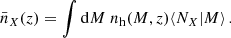
where we omitted the explicit dependence on redshift. For the symmetric perturbation theory kernels,  , we refer to Bernardeau et al. (2002). The trispectrum relates to the nG term in Equation (4) for k1=−k2 and k2=−k4. Lastly, we specify the SSC (Takada & Hu 2013; Krause & Eifler 2017; Barreira et al. 2018), i.e. the second term in Equation (4):
 (31)
(31)
We note that k1 corresponds to the correlated pair A1,A2 and k2 to A3,A4. The responses are given as
![Mathematical equation: $$ \begin{aligned} \frac {\partial P_{A_1A_2}}{\partial \delta _\mathrm {bg}}(k,z) = &\; \left [\frac {68}{21} - \frac {1}{3}\frac {\mathrm {d}\log k^3 P_{A_1A_2}(k,z)}{\mathrm {d}\log k} \right ] I^1_{1,A_1}(k,z)I^1_{1,A_2}(k,z)P_\mathrm {lin}(k,z) \\ & + I^1_{2,A_1A_2}(k,k,z) - \left ([b_{A_1} + b_{A_2}] P_{A_1A_2}(k,z)\right )_{\mathrm {if\;} {A_1, A_2\neq \mathrm {m}}}\,. \end{aligned} $$](/articles/aa/full_html/2025/07/aa52592-24/aa52592-24-eq48.gif) (32)
(32)
We note that in the last term the contribution of  vanishes if the mean of Ai is not constructed in the survey window, such as for CS. The responses are defined with respect to fluctuations in the background, ‘bg’, matter field, which can be calculated directly from the survey mask and its spherical harmonic decomposition:
 (33)
(33)
The bracket notation (A1A2) denotes the footprint of the survey over which the summary statistic between the tracers A1 and A2 has been evaluated. As expected  as
as  due to statistical homogeneity and isotropy. If the survey footprint is not available via a mask file, we assume a circular footprint and follow Li et al. (2014)
![Mathematical equation: $$ \sigma ^2_{\mathrm {bg},(A_1A_2)(A_3A_4)}(z) = \chi (z)^2\int \frac {k\mathrm {d}k}{(2\uppi )^2} P_\mathrm {lin}(k,z)\left [\frac {2{\mathrm {J}}_1(k\chi (z)\theta _\mathrm {s})}{k\chi (z)\theta _\mathrm {s}}\right ]^2\,, $$](/articles/aa/full_html/2025/07/aa52592-24/aa52592-24-eq53.gif) (34)
(34)
with a cylindrical Bessel function, J1, and the survey size  , such that the larger survey area is used.
4. Harmonic space covariance
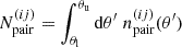
The components outlined in Section 3 can now be translated to harmonic space through the Limber projection, as given in Equation (10). To achieve this, the line-of-sight weights,  , still have to be specified. The OneCovariance code typically employs two types of tracers, ai, which can represent either the CS measured from a source galaxy sample, denoted mi or the positions of a lens galaxy sample gi, respectively. In the literature, different terminologies exist. With a ‘source’ we refer to a galaxy whose lensed ellipticity will be used. Conversely, a ‘lens’ is a galaxy whose position will be used. To summarise, GC would be the ‘lens’-‘lens’ auto-correlation, CS the ‘source’-‘source’ auto-correlation and GGL the ‘source’-‘lens’ cross-correlation. The index i labels the tomographic bin of the corresponding sample. With this, the weight functions assume the following form
 (35)
(35)
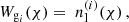
![Mathematical equation: $$ W_{\mathrm {m}_i}(\chi ) = \frac {3f_\mathrm {K}(\chi )\Omega _\mathrm {m}}{2\chi ^2_\mathrm {H}a}\int _\chi ^\mathrm {\chi _\mathrm {H}}\mathrm {d}\chi ^\prime \;\frac {f_\mathrm {K}(\chi ^\prime - \chi )}{f_\mathrm {K}(\chi ^\prime )}n^{(i)}_\mathrm {s}(\chi ) - A_\mathrm {IA}\left [\frac {1+z(\chi )}{1+z_\mathrm {pivot}}\right ]^{\eta _\mathrm {IA}}\frac {C_1\rho _\mathrm {cr}\Omega _\mathrm {m}}{D_+[a(\chi )]}n^{(i)}_\mathrm {s}(\chi ) \,. $$](/articles/aa/full_html/2025/07/aa52592-24/aa52592-24-eq57.gif) (36)
(36)
Here χH is the co-moving distance to the horizon,  and
and  are the normalised redshift distributions of the lens- and source sample respectively. D+(a) is the linear growth factor and C1ρcr≈0.0134. The second term in the
  weight function corresponds to the non-linear linear alignment model (NLA, Hirata & Seljak 2004; Bridle & King 2007) with alignment amplitude AIA and redshift dependence ηIA at a pivot redshift zpivot. There are two remarks in order here: (i) The NLA model is the fiducial choice of the OneCovariance code. However, the user can include any alignment model (at least in the dominating Gaussian part) by providing the corresponding Cℓ as input. Therefore, including, for example, the Tidal Alignment-Tidal Torquing (TATT, Blazek et al. 2019) is straightforwardly done (see Section 6). (ii) For the fiducial NLA model, any lensing tracer automatically assumes a linear response to the non-linearly evolved density field. Consequently, the alignment is also modelled in the SSC and NG terms of the covariance matrix and not just in the Gaussian part.
In addition to the cosmological signal ( ), observed modes (
 ) contain a noise realisation (
 ) since the continuous field is sampled by a finite number of tracers (galaxies),
 (37)
(37)
with  and noise statistic
  , as the noise in different maps is uncorrelated, and the noise is scale independent. Strictly speaking, this relation only holds for full sky coverage where all the modes are independent. Therefore, the noise component will be treated in real space directly to avoid this complication. We come back to this issue in Section 5. The factor
  determines the overall noise level depending on the observable under consideration:
 (38)
(38)
Here  is the average number density of the tracers and
  is the single component ellipticity dispersion of the sources. The standard idealised angular power spectrum estimator at each multipole is defined as
 (39)
(39)
such that
 (40)
(40)
In the flat sky approximation, the same estimator assumes the form
 (41)
(41)
where we defined an annulus in Fourier space with volume 2πℓΔℓ, so that the number of available modes over the survey area As is
 (42)
(42)
where Δℓ≪ℓ was assumed. The covariance matrix between two estimators is then, again by noting that ℓ1 corresponds to the pair a1,a2 and ℓ2 corresponds to the pair a3,a4:
![Mathematical equation: $$ \begin{aligned} \mathrm {Cov}[{\hat {C}}_{a_1a_2}(\ell _1){\hat {C}}_{a_3a_4}(\ell _2)] = & \;\frac {1}{A_{(12)}N_\mathrm {modes}(\ell _1)}\frac {1}{A_{(34)}N_\mathrm {modes}(\ell _2)}\sum _{{\tilde {\boldsymbol {\ell }}}_1\in \ell _{1,\mathrm {ring}}}\sum _{{\tilde {\boldsymbol {\ell }}}_2\in \ell _{2,\mathrm {ring}}}\left (\left \langle {\hat {a}}^1_{\boldsymbol {\ell }_1}{\hat {a}}^2_{-\boldsymbol {\ell }_1} {\hat {a}}^3_{\boldsymbol {\ell }_2}{\hat {a}}^4_{-\boldsymbol {\ell }_2}\right \rangle - \left \langle {\hat {a}}^1_{\boldsymbol {\ell }_1}{\hat {a}}^2_{-\boldsymbol {\ell }_1}\right \rangle \langle {\hat {a}}^3_{\boldsymbol {\ell }_2}{\hat {a}}^4_{-\boldsymbol {\ell }_2}\rangle \right )\\ = & \;\frac {1}{N_\mathrm {modes}(\ell _1)}\frac {1}{N_\mathrm {modes}(\ell _2)}\sum _{{\tilde {\boldsymbol {\ell }}}_1\in \ell _{1,\mathrm {ring}}}\left ({C}_{a_1a_3}(\ell _1){C}_{a_2a_4}(\ell _2) + {C}_{a_1a_4}(\ell _1){C}_{a_2a_3}(\ell _2)\right ) \delta ^\mathrm {K}_{\ell _1\ell _2} \\ & + \;\frac {1}{\mathrm {max}(A_{(12)}A_{(34)})N_\mathrm {modes}(\ell _1)N_\mathrm {modes}(\ell _2)}\sum _{{\tilde {\boldsymbol {\ell }}}_1\in \ell _{1,\mathrm {ring}}}\sum _{{\tilde {\boldsymbol {\ell }}}_2\in \ell _{2,\mathrm {ring}}}T^{(a_1a_2)(a_3a_4)}(\boldsymbol {\ell }_1, -\boldsymbol {\ell }_1,\boldsymbol {\ell }_2,-\boldsymbol {\ell }_2)\,. \end{aligned} $$](/articles/aa/full_html/2025/07/aa52592-24/aa52592-24-eq75.gif) (43)
(43)
Here Aij,s is the survey area over which the angular power spectrum of the two fields ai and aj is estimated. Furthermore, T(a1a2)(a3a4)(ℓ1,−ℓ1,ℓ2,−ℓ2) is the trispectrum, see Equation (49) below. We note that the area cancels out in the Gaussian term due to the application of two correlators (compare Equation (D.3)).
Assuming that the angular power spectra do not vary significantly over the bandwidth of the ring ℓring, the Gaussian term in the flat sky approximation is given by the commonly used expression
![Mathematical equation: $$ \mathrm {Cov}_\mathrm {G}[{\hat {C}}_{a_1a_2}(\ell _1){\hat {C}}_{a_3a_4}(\ell _2)] \approx \frac {4\uppi \delta ^{\mathrm {K}}_{\ell _1\ell _2}}{\mathrm {max}(A_{(12)}A_{(34)})2\ell _1\Delta \ell _1} \left [{C}_{a_1a_3}(\ell _1){C}_{a_2a_4}(\ell _2) + {C}_{a_1a_4}(\ell _1){C}_{a_2a_3}(\ell _2)\right ]\,. $$](/articles/aa/full_html/2025/07/aa52592-24/aa52592-24-eq76.gif) (44)
(44)
This can be compared to the full sky version of the Gaussian term which, at each multipole, is given by
![Mathematical equation: $$ \mathrm {Cov}_\mathrm {G}[{\hat {C}}_{a_1a_2}(\ell _1){\hat {C}}_{a_3a_4}(\ell _2)] = \frac {4\uppi \delta ^{\mathrm {K}}_{\ell _1\ell _2}}{\mathrm {max}(A_{(12)}A_{(34)})(2\ell _1+1)}\left [{C}_{a_1a_3}(\ell _1){C}_{a_2a_4}(\ell _2) + {C}_{a_1a_4}(\ell _1){C}_{a_2a_3}(\ell _2)\right ]\,, $$](/articles/aa/full_html/2025/07/aa52592-24/aa52592-24-eq77.gif) (45)
(45)
where we introduced the sky fraction max(A(12)A(34))/(4π) to mimic incomplete sky coverage (van Uitert et al. 2018). Averaging over multipole bands and assuming again that the spectra do not vary significantly across the bands yields
![Mathematical equation: $$ \mathrm {Cov}_\mathrm {G}[{\hat {C}}_{a_1a_2}(\ell _1){\hat {C}}_{a_3a_4}(\ell _2)] \approx \frac {4\uppi \delta ^{\mathrm {K}}_{\ell _1\ell _2}}{\mathrm {max}(A_{(12)}A_{(34)})(2\ell _1+1)\Delta \ell _1}\left [{C}_{a_1a_3}(\ell _1){C}_{a_2a_4}(\ell _2) + {C}_{a_1a_4}(\ell _1){C}_{a_2a_3}(\ell _2)\right ]\,, $$](/articles/aa/full_html/2025/07/aa52592-24/aa52592-24-eq78.gif) (46)
(46)
which is the same expression as Equation (44) for ℓ≫1, as expected. Equation (45) amounts to the splitting discussed in Equation (6). We now turn back to the connected term in Equation (43):
![Mathematical equation: $$ \mathrm {Cov}_\mathrm {nG}[{\hat {C}}_{a_1a_2}(\ell _1){\hat {C}}_{a_3a_4}(\ell _2)] = \frac {1}{\mathrm {max}(A_{(12)}A_{(34)})}\int _{{\tilde {\ell }}_1\in \ell _1}\frac {\mathrm {d}^2{\tilde {\ell }}_1}{A(\ell _1)}\int _{{\tilde {\ell }}_2\in \ell _2}\frac {\mathrm {d}^2{\tilde {\ell }}_2}{A(\ell _2)} T^{(a_1a_2)(a_3a_4)}({\tilde {\boldsymbol {\ell }}}_1, -{\tilde {\boldsymbol {\ell }}}_1,{\tilde {\boldsymbol {\ell }}}_2,-{\tilde {\boldsymbol {\ell }}}_2)\,, $$](/articles/aa/full_html/2025/07/aa52592-24/aa52592-24-eq79.gif) (47)
(47)
where we moved to the continuous version of the two-dimensional Fourier transformation. All trispectra are projected with the Limber projection and the angular average is carried out already in k-space:
 (48)
(48)
where
 (49)
(49)
where ϕℓ is the angle between the two wave vectors k1,2 in the plane perpendicular to the line of sight. Altogether, the covariance in harmonic space is given by
![Mathematical equation: $$ \mathrm {Cov}[{\hat {C}}_{a_1a_2}(\ell _1){\hat {C}}_{a_3a_4}(\ell _2)] = \mathrm {Cov}_\mathrm {G}\left [{\hat {C}}_{a_1a_2}(\ell _1){\hat {C}}_{a_3a_4}(\ell _2)\right ] + \frac {1}{\mathrm {max}(A_{(12)}A_{(34)})} T^{(a_1a_2)(a_3a_4),\; \mathrm {nG}}_{\ell _1\ell _2} + T^{(a_1a_2)(a_3a_4),\; \mathrm {SSC}}_{\ell _1\ell _2}\; $$](/articles/aa/full_html/2025/07/aa52592-24/aa52592-24-eq82.gif) (50)
(50)
at each multipole ℓ. For an ℓ-band averaged version, we use Equations (44) and (47). This is only important if a pure ℓ-space covariance is required, since the averaging over scales is taken care of when mapping the theoretical ℓ-space covariance to the observables in the next section.
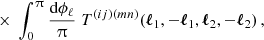
5. From harmonic space to observables
Whilst theoretical modelling is most straightforward in harmonic space, the theoretical power spectra, denoted as C(ℓ), are technically defined solely on the full sky. As real surveys typically cover only a portion of the sky, the advantage of harmonic space diminishes. This is because different ℓ modes become intermingled, and the partial sky Cℓ, often referred to as pseudo-Cℓ, are derived from the full-sky Cℓ via convolution with the mode mixing matrix (see e.g. Hivon et al. 2002; Kogut et al. 2003; Reinecke & Seljebotn 2013; Elsner et al. 2017; Alonso et al. 2019).
Deconvolution may not always be feasible for intricate sky masks, rendering the Cℓ indirectly observable and serving primarily as an intermediary product. Another challenge arises from the projection, as outlined in Equation (7), which combines various physical scales if the window function WA(χ) possesses broad support in the co-moving distance. Additionally, the shear field's spin-2 nature permits its separation into E and B modes.
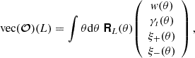
To mitigate these difficulties, a variety of summary statistics are available, including the probes of the classical 3×2-point analysis: GC, CS, and GGL. Accordingly, the OneCovariance code can accommodate diverse inputs for three-dimensional power spectra, angular power spectra, or weight functions for the projection, rendering the discussion applicable to all general tracers or summary statistics of two-point functions in the LSS. In a broader context, any two-point summary statistic represents a linear transformation of the underlying two-point statistic in harmonic space, as nonlinear transformations would involve contributions from higher-order cumulants. Therefore, we write the summary statistic  between two tracers a1 and a2 as
 (51)
(51)
Here L can be a discrete label or a continuous variable for some Fourier filter WL(ℓ). Importantly,  , concatenates all unique
  into a vector which is mapped to the new summary statistic
  via the aforementioned linear map. Throughout this section, we omit the formal integration limits from zero to infinity, but all integrals over ℓ are understood to run over this range if not specified differently. It should be noted that the internal structure of
  depends on the underlying fields a1 and a2. If the spin of a1 and a2 is non-zero, such as for CS, they both consist of two complex components so that C is a real 2×2 matrix given by
 (52)
(52)
on the full sky for a homogeneous and isotropic random field. The CS submatrix of WL(ℓ) is a symmetric and real 2×2 matrix with two independent contributions: the curl-free E-mode signal and the divergence-free B-mode signal, where we assume that there is no measurable contribution to the EB spectrum. We thus bundle the combined C(ℓ) of all probes (for a standard 3×2 analysis) in a vector by using the notation of Equation 35 and 36
 {{\scriptstyle:\!\!}=} (C_\mathrm {gg},C_\mathrm {gm},C_\mathrm {mm,EE},C_\mathrm {mm,BB})^\mathrm {T}(\ell )\,, $$](/articles/aa/full_html/2025/07/aa52592-24/aa52592-24-eq90.gif) (53)
(53)
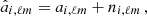
where tomographic bin indices have been omitted for clarity. The resulting summary statistics are bundled in the same fashion:
 {{\scriptstyle:\!\!}=} ({{\cal {{O}}}}_\mathrm {gg},{{\cal {{O}}}}_\mathrm {gm}, {{\cal {{O}}}}_\mathrm {mm,EE}, {{\cal {{O}}}}_\mathrm {mm,BB})^\mathrm {T}(L)\,. $$](/articles/aa/full_html/2025/07/aa52592-24/aa52592-24-eq91.gif) (54)
(54)
In this manner, we can express the transformation from Fourier space to the summary statistic using Equation (51). Real space correlation functions decouple the shot or shape noise contribution from different scales, L. Furthermore, the shot or shape noise contribution can be precisely estimated from the data itself, regardless of complex masks. To leverage those properties the shot or shape noise levels defined in Equation (38), which only apply to full-sky data, are improved by also providing a relation between real space correlation (see Section 5.2) and the observables. Therefore, we also require the following correlation for some real space filter function RL(θ)
 (55)
(55)
with the real space correlation functions defined via Hankel transformations of the angular power spectrum, Equation (8). For CS, this amounts to the two correlation functions (Bartelmann & Schneider 2001)
![Mathematical equation: $$ \xi _+^{(ij)}(\theta ) = \int \frac { \ell \mathrm {d}\ell }{2 \uppi } \; \left [{\cal {{P}}}_{\epsilon _i\epsilon _j,\mathrm {E}}(\ell ) + {\cal {{P}}}_{\epsilon _i\epsilon _j,\mathrm {B}}(\ell )\right ] \; {\mathrm {J}}_0(\ell \theta )\,, $$](/articles/aa/full_html/2025/07/aa52592-24/aa52592-24-eq93.gif) (56)
(56)
![Mathematical equation: $$ \xi _-^{(ij)}(\theta ) = \int \frac {\ell \mathrm {d}\ell }{2 \uppi } \; \left [{\cal {{P}}}_{\epsilon _i\epsilon _j,\mathrm {E}}(\ell ) - {\cal {{P}}}_{\epsilon _i\epsilon _j,\mathrm {B}}(\ell )\right ] \; \mathrm {J}_4(\ell \theta )\,, $$](/articles/aa/full_html/2025/07/aa52592-24/aa52592-24-eq94.gif) (57)
(57)
where Jμ is a cylindrical Bessel function of the first kind of order μ. The angular power spectrum  was decomposed into an E and B-mode component. Recall that we explicitly use the noise-free version of the angular power spectra here as defined in the estimator in Equation (40). For GGL one measures the tangential shear correlation function
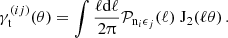 (58)
(58)
The galaxy correlation function can be calculated as
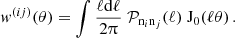 (59)
(59)
We note that these are all the continuous versions and large multipole approximations of the discrete transformations. We continue to review the definitions of the three most commonly used summary statistics (real space correlation functions, band powers and COSEBIs) and the corresponding covariances. A more detailed discussion of the general setting can be found in Appendix I.
5.1. Multiplicative shear bias
Shear measurements for source samples are calibrated on image simulations (see e.g. Kannawadi et al. 2019; Li et al. 2023). Residual biases are captured in a multiplicative and additive shear bias, which needs to be propagated into the cosmological inference. We assume that there are no residual spatial patterns in the additive contribution (e.g. from point-spread function leakage) and hence no correlation with the cosmological signal. Thus, the only source of error which has to be propagated in the covariance is the multiplicative m-correction. The residual error on the multiplicative shear bias after calibration is labelled  for source bin a1. Considering the multiplicative shear bias uncertainty as an additive contribution to the covariance matrix (Joachimi et al. 2021), so that
![Mathematical equation: $$ \mathrm {Cov}_\mathrm {mult}\left [{\cal {{O}}}_{a_1a_2} (L_1), {\cal {{O}}}_{a_3a_4} (L_2) \right ] = {\cal {{O}}}_{a_1a_2} (L_1){\cal {{O}}}_{a_3a_4} (L_2)\left [\sigma ^{a_1}_\mathrm {m}\sigma ^{a_3}_\mathrm {m} + \sigma ^{a_1}_\mathrm {m}\sigma ^{a_4}_\mathrm {m}+ \sigma ^{a_2}_\mathrm {m}\sigma ^{a_3}_\mathrm {m}+\sigma ^{a_2}_\mathrm {m}\sigma ^{a_4}_\mathrm {m}\right ]\,. $$](/articles/aa/full_html/2025/07/aa52592-24/aa52592-24-eq99.gif) (60)
(60)
This approximation holds for  , for 〈m〉=0〉 after correction and fully correlated m-bias corrections across tomographic bins. We note that only source samples have a
  . by definition. The assumption 〈m〉=0〉 is not crucial for the covariance, as this can be addressed by directly shifting the data vector while keeping the covariance unchanged (Li et al. 2023).
5.2. Real space correlation functions
When propagating the covariance matrix from the angular power spectra to the real space correlation functions in Equations (56), (57), (58), and (59) we take into account that the correlation functions are measured over finite angular separation bins centred at  with boundaries [θl,i,θu,i], the bin average needs to be carried out explicitly. To capture the different weight functions, we use the notation from Joachimi et al. (2021)
![Mathematical equation: $$ {\cal {{K}}}_\mu \left (\ell \bar {\theta }_i\right ):= \frac {2}{\theta _{{\mathrm {u}},i}^2 - \theta _{{\mathrm {l}},i}^2 }\, \int _{\theta _{{\mathrm {l}},i}}^{\theta _{{\mathrm {u}},i}} \mathrm {d} \theta '\, \theta ' {\mathrm {J}}_\mu (\ell \theta ') = \frac {2}{{\left ({ \theta _{{\mathrm {u}},i}^2 - \theta _{{\mathrm {l}},i}^2 } \right )} \ell ^2}\, \times \, \left\{ \begin {array}{ll} \left [{x {\mathrm {J}}_1(x)} \right ]_{\ell \theta _{{\mathrm {l}},i}}^{\ell \theta _{{\mathrm {u}},i}} & \mu =0\,, \\ \left [{ -x {\mathrm {J}}_1(x) - 2 {\mathrm {J}}_0(x) } \right ]_{\ell \theta _{{\mathrm {l}},i}}^{\ell \theta _{{\mathrm {u}},i}} & \mu =2\,, \\ \left [{ {\left ({x -\frac {8}{x}} \right )} {\mathrm {J}}_1(x) - 8 {\mathrm {J}}_2(x) } \right ]_{\ell \theta _{{\mathrm {l}},i}}^{\ell \theta _{{\mathrm {u}},i}} & \mu =4\,. \end {array} \right .\;, $$](/articles/aa/full_html/2025/07/aa52592-24/aa52592-24-eq103.gif) (61)
(61)
ignoring the weights of the pair counts (Asgari et al. 2019). The set of possible correlation functions is denoted accordingly in a compact form (see the notation used in Joachimi et al. 2021):

We note that w and ξ+ have the same weight function. As discussed, the Gaussian covariance is split into three contributions as in Equation (6). For the pure shot/shape noise (sn) term, this procedure is a numerical necessity, as an ℓ-independent integrand will lead to a δD-contribution to the covariance. Since we reconsider the idealised term in Appendix F for real space correlation functions, this splitting is also necessary here as the ‘mix’ term is the most important while also still being a somewhat uncertain term in the analytical covariance modelling. Numerically, it is, however, usually advantageous to combine the sample variance (‘sva’) and mixed terms to speed up the convergence of the integrals.
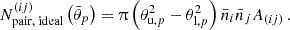
Using Equation (51), the definitions of the weights above and Equation (50), the ‘sva’ term is given by
![Mathematical equation: $$ {\mathrm {Cov}}_{\mathrm {G, sva}} {\left [{\Xi _\mu ^{(ij)}\left (\bar {\theta }_p\right );\, \Xi _\nu ^{(mn)}\left (\bar {\theta }_q\right )} \right ]} = \frac {1}{2 \uppi \; \mathrm {max}(A_{(ij)}A_{(mn)}) } \int \!\mathrm {d}\ell \, \ell \; {\cal {{K}}}_\mu \left (\ell \bar {\theta }_p\right ) {\cal {{K}}}_\nu \left (\ell \bar {\theta }_q\right ) {\left [{ {\cal {{P}}}_{im}(\ell ) {\cal {{P}}}_{jn}(\ell ) + {\cal {{P}}}_{in}(\ell ) {\cal {{P}}}_{jm}(\ell ) } \right ]} \,, $$](/articles/aa/full_html/2025/07/aa52592-24/aa52592-24-eq105.gif) (62)
(62)
where the tomographic indices i,j,m,n label either a source or a lens sample. We measure all areas from a binary healpix mask down to a certain angular scale so that masked stars and other features only reduce the effective number density and not the survey area. This assumption is valid as long as this dilution scale is smaller than the smallest scale over which the cosmological signal is measured. Typically, one assumes Nside=4096 for the healpix (Górski et al. 2005) evaluation, corresponding to a pixel size of just below one arcmin.
In an ideal survey, the pure noise contribution is just the product of the two individual noise contributions, Equation (38), to the measurement of the two-point statistic amounting to a term proportional to the number of (non-unique) pairs in bin  :
:
 (63)
(63)
This equation is accurate in the absence of survey boundaries. For finite areas, however, the number of pairs as a function of angular scale differs from the expected ∝θ2 scaling. To obtain a more accurate prescription of the pure shot noise contribution, the number of pairs is directly measured at the catalogue level, providing  . Altogether,
![Mathematical equation: $$ {\mathrm {Cov}}_{\mathrm {G, sn}} {\left [{\Xi _\mu ^{(ij)}\left (\bar {\theta }_p\right );\, \Xi _\nu ^{(mn)}\left (\bar {\theta }_q\right )} \right ]} =\delta ^\mathrm {K}_{\mu \nu } \delta ^\mathrm {K}_{\bar {\theta }_p \bar {\theta }_q} {\left ({\delta ^\mathrm {K}_{im} \delta ^\mathrm {K}_{jn} + \delta ^\mathrm {K}_{in} \delta ^\mathrm {K}_{jm} } \right )} \frac {{\cal {{T}}}_{(ij)(mn)}^{\mathrm {sn}} }{N_{\mathrm {pair}}^{(ij)}\left (\bar {\theta }_p\right ) } \,, $$](/articles/aa/full_html/2025/07/aa52592-24/aa52592-24-eq109.gif) (64)
(64)
where we defined the noise levels
 (65)
(65)
We recall that ‘source’ refers to the galaxy shape and ‘lens’ to the galaxy position being used. Furthermore, we note that the Latin indices carry a hidden label “lens” or “source” so that  only when both indices come from the same set. It should be noted that, while we use in the equations here the non-unique pairs, for any correlation measurement, however, only the unique pairs are relevant. This is accounted for in the covariance calculations. Since this often leads to confusion, let us use tomographic clustering with equi-populated bins as an example. The noise level will always be ∼1/N2, with N being the number of galaxies in each bin. For auto-correlations, however, the Kronecker symbols in the brackets in Equation (64) make sure that only unique pairs are counted, effectively increases the covariance by a factor of two. In contrast, for cross-correlations, the N2 is actually the number of unique pairs.
The mixed term is calculated in the same fashion as the sample variance contribution, Equation (62):
![Mathematical equation: $$ {\mathrm {Cov}}_{\mathrm {G, mix}} {\left [{\Xi _\mu ^{(ij)}\left (\bar {\theta }_p\right );\, \Xi _\nu ^{(mn)}\left (\bar {\theta }_q\right )} \right ]} = \delta _{jn}\, \frac {{\cal {{T}}}_j^{\mathrm {mix}}}{2 \uppi n_{\mathrm {eff}}^{(j)}\, \mathrm {max}(A_{(ij)}A_{(mn)}) } \int \mathrm {d} \ell \, \ell \; {\cal {{K}}}_\mu \left (\ell \bar {\theta }_p\right ) {\cal {{K}}}_\nu \left (\ell \bar {\theta }_q\right )\, {\cal {{P}}}_{im}(\ell ) + \mbox {3 perm.}\,, $$](/articles/aa/full_html/2025/07/aa52592-24/aa52592-24-eq112.gif) (66)
(66)
The noise level of the mixed term is defined as
 (67)
(67)
We note that this is an idealised setting for a rescaled full sky survey without a complicated mask. In Appendix F we revisit this term using the triplet counts of a catalogue to estimate the effect on the covariance and cosmological inference.
The non-Gaussian covariance and SSC are
![Mathematical equation: $$ {\mathrm {Cov}}_{\mathrm {NG/SSC}} {\left [{\Xi ^{(ij)}_\mu \left (\bar {\theta }_p\right );\, \Xi ^{(mn)}_\nu \left (\bar {\theta }_q\right )} \right ]} = \; \frac {1}{4 \uppi ^2 } \int \mathrm {d} \ell _1\, \ell _1\; {\cal {{K}}}_\mu \left (\ell _1 \bar {\theta }_p\right ) \int \mathrm {d} \ell _2\, \ell _2\; {\cal {{K}}}_\nu \left (\ell _2 \bar {\theta }_q\right ) $$](/articles/aa/full_html/2025/07/aa52592-24/aa52592-24-eq114.gif) (68)
(68)
5.3. Bandpowers
We define the bandpower signal their weights and further ingredients in Appendix G and focus on the covariance here. In contrast to the real space approach in Joachimi et al. (2021) we calculate the bandpower covariance from Fourier space directly using Equations (G.13), (G.14), (G.15), and (G.16). This is done to resemble the analytical calculations of the predicted signal and for numerical stability and speed. In complete analogy to the real space correlation functions, we write
![Mathematical equation: $$ {\mathrm {Cov}}_{\mathrm {G, sva}} {\left [{{\cal {{C}}}^{(ij)}_{\mu }(L_1), {\cal {{C}}}^{(mn)}_{\nu }(L_2)} \right ]} = \frac {2 \uppi }{{\cal {{N}}}_{L_1}{\cal {{N}}}_{L_2} \mathrm {max}(A_{(ij)}A_{(mn)}) } \int \mathrm {d}\ell \, \ell \; {\cal {{W}}}^{L_1}_{\mu }(\ell ) {\cal {{W}}}^{L_2}_{\nu }(\ell ) [{\cal {{P}}}_{im}(\ell ) {\cal {{P}}}_{jn}(\ell ) + {\cal {{P}}}_{in}(\ell ) {\cal {{P}}}_{jm}(\ell )] $$](/articles/aa/full_html/2025/07/aa52592-24/aa52592-24-eq116.gif) (69)
(69)
![Mathematical equation: $$ {\mathrm {Cov}}_{\mathrm {G, mix}} {\left [{{\cal {{C}}}^{(ij)}_{\mu }(L_1), {\cal {{C}}}^{(mn)}_{\nu }(L_2)} \right ]} = \delta _{jn}\, \frac {2 \uppi \;{\cal {{T}}}_j^{\mathrm {mix}}}{{\cal {{N}}}_{L_1}{\cal {{N}}}_{L_2}n_{\mathrm {eff}}^{(j)}\, \mathrm {max}(A_{(ij)}A_{(mn)}) } \int \mathrm {d} \ell \, \ell \; {\cal {{W}}}^{L_1}_{\mu }(\ell ) {\cal {{W}}}^{L_2}_{\nu }(\ell )\, {\cal {{P}}}_{im}(\ell ) + \mbox {3 perm.} \,, $$](/articles/aa/full_html/2025/07/aa52592-24/aa52592-24-eq117.gif)
assuming that the cosmological B-mode signal vanishes. The following shorthand notation for the weights was used:
 (70)
(70)
To properly incorporate the pair counts the pure shot-noise contributions are calculated from real space:
![Mathematical equation: $$ {\mathrm {Cov}}_{\mathrm {G, sn}} {\left [{{\cal {{C}}}^{(ij)}_{\mu }(L_1), {\cal {{C}}}^{(mn)}_{\nu }(L_2)} \right ]} = \; \frac {\uppi ^2\delta ^\mathrm {K}_{\mu \nu }}{{\cal {{N}}}_{L_1}{\cal {{N}}}_{L_2}} \left (\delta ^\mathrm {K}_{im}\delta ^\mathrm {K}_{jn} + \delta ^\mathrm {K}_{in}\delta ^\mathrm {K}_{jm}\right ) \int \frac {\theta ^2\mathrm {d}\theta }{n^{(ij)}_\mathrm {pair}(\theta )} $$](/articles/aa/full_html/2025/07/aa52592-24/aa52592-24-eq119.gif) (71)
(71)
The differential pair counts,  , are defined such that the number of pairs,
  , in an angular bin [θl,θu] is
 (72)
(72)
directly from the, possibly weighted, pair counts of the catalogue. Lastly, the nG and SSC terms can be calculated as follows:
![Mathematical equation: $$ {\mathrm {Cov}}_{\mathrm {NG}} {\left [{{\cal {{C}}}^{(ij)}_{\mu }(L_1), {\cal {{C}}}^{(mn)}_{\nu }(L_2)} \right ]} = \frac {1}{{\cal {{N}}}_{L_1}{\cal {{N}}}_{L_2} \mathrm {max}(A_{(ij)}A_{(mn)}) } \int \mathrm {d}\ell _1\, \ell _1{\cal {{W}}}^{L_1}_{\mu }(\ell _1)\int \mathrm {d}\ell _2\, \ell _2\; {\cal {{W}}}^{L_2}_{\nu }(\ell _2) $$](/articles/aa/full_html/2025/07/aa52592-24/aa52592-24-eq124.gif) (73)
(73)
![Mathematical equation: $$ {\mathrm {Cov}}_{\mathrm {SSC}} {\left [{{\cal {{C}}}^{(ij)}_{\mu }(L_1), {\cal {{C}}}^{(mn)}_{\nu }(L_2)} \right ]} = \frac {1}{{\cal {{N}}}_{L_1}{\cal {{N}}}_{L_2}} \int \mathrm {d}\ell _1\, \ell _1{\cal {{W}}}^{L_1}_{\mu }(\ell _1)\int \mathrm {d}\ell _2\, \ell _2\; {\cal {{W}}}^{L_2}_{\nu }(\ell _2) T^{(ij)(mn)}_\mathrm {SSC}({\ell _1,\ell _2})\,. $$](/articles/aa/full_html/2025/07/aa52592-24/aa52592-24-eq126.gif) (74)
(74)
5.4. COSEBIs and Ψ statistics
Due to the similar structure of the COSEBIs we repeat the same calculation as for the band power covariance, i.e. projecting all terms from harmonic space except for the pure shot noise term. With the definition of COSEBIs, see Appendix H, this yields the following:
![Mathematical equation: $$ {\mathrm {Cov}}_{\mathrm {G, sva}} {\left [{E^{(ij)}_{a}, E^{(mn)}_{b}} \right ]} =\; \frac {1}{2\uppi \;\mathrm {max}(A_{(ij)}A_{(mn)}) } \int \mathrm {d}\ell \, \ell \; { W}_{a}(\ell ) { W}_{b}(\ell ) {\left [{ {\cal {{P}}}_{im}(\ell ) {\cal {{P}}}_{jn}(\ell ) + {\cal {{P}}}_{in}(\ell ) {\cal {{P}}}_{jm}(\ell ) } \right ]} $$](/articles/aa/full_html/2025/07/aa52592-24/aa52592-24-eq127.gif) (75)
(75)
![Mathematical equation: $$ {\mathrm {Cov}}_{\mathrm {G, mix}} {\left [{E^{(ij)}_{a}, E^{(mn)}_{b}} \right ]} =\; \delta _{jn}\, \frac {\;{\cal {{T}}}_j^{\mathrm {mix}}}{2 \uppi \; n_{\mathrm {eff}}^{(j)}\, \mathrm {max}(A_{(ij)}A_{(mn)}) } \int \mathrm {d} \ell \, \ell \; { W}_{a}(\ell ) { W}_{b}(\ell )\, {\cal {{P}}}_{im}(\ell ) + {\textrm {3 perm.}} $$](/articles/aa/full_html/2025/07/aa52592-24/aa52592-24-eq128.gif) (76)
(76)
![Mathematical equation: $$ {\mathrm {Cov}}_{\mathrm {NG}} {\left [{E^{(ij)}_{a}, E^{(mn)}_{b}} \right ]} = \; \frac {1}{2\uppi \; \mathrm {max}(A_{(ij)}A_{(mn)}) } \int \mathrm {d}\ell _1\, \ell _1{ W}_{a}(\ell _1)\int \mathrm {d}\ell _2\, \ell _2\; { W}_{b}(\ell _2) \int _0^\uppi \frac {\mathrm {d} \phi _\ell }{\uppi } \; T^{(ij)(mn)}(\boldsymbol {\ell }_1,-\boldsymbol {\ell }_1,\boldsymbol {\ell }_2,-\boldsymbol {\ell }_2)\,, $$](/articles/aa/full_html/2025/07/aa52592-24/aa52592-24-eq129.gif) (77)
(77)
![Mathematical equation: $$ {\mathrm {Cov}}_{\mathrm {SSC}} {\left [{E^{(ij)}_{a}, E^{(mn)}_{b}} \right ]} = \; \frac {1}{2\uppi \;} \int \mathrm {d}\ell _1\, \ell _1{ W}_{a}(\ell _1)\int \mathrm {d}\ell _2\, \ell _2\; { W}_{b}(\ell _2) T^{(ij)(mn)}_\mathrm {SSC}({\ell _1,\ell _2}) $$](/articles/aa/full_html/2025/07/aa52592-24/aa52592-24-eq130.gif) (78)
(78)
![Mathematical equation: $$ {\mathrm {Cov}}_{\mathrm {G, sn}} {\left [{E^{(ij)}_{a}, E^{(mn)}_{b}} \right ]} =\; \frac {\sigma ^2_{\epsilon _1,\;i}\sigma ^2_{\epsilon _1,\;j} }{2} \left (\delta ^\mathrm {K}_{im}\delta ^\mathrm {K}_{jn} + \delta ^\mathrm {K}_{in}\delta ^\mathrm {K}_{jm}\right )\int \frac {\theta ^2\mathrm {d}\theta }{n^{(ij)}_\mathrm {pair}(\theta )}\left [{T}_{+a}(\theta ){ T}_{+b}(\theta ) + {T}_{-a}(\theta ){ T}_{-b}(\theta )\right ]\,. $$](/articles/aa/full_html/2025/07/aa52592-24/aa52592-24-eq131.gif) (79)
(79)
The expressions of the covariance of Ψ statistics is in full analogy to Equations (75), (76), (77), (78) (79).
5.5. Stellar mass function
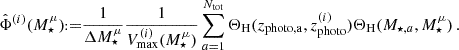
To complement the halo model, we also implement the SMF covariance, Equation (20), which was already used in Dvornik et al. (2023). For a flux-limited sample, we consider the standard Vmax(M★)-estimator, where Vmax is the maximum volume out to which a galaxy with a given mass can be observed given the limiting magnitude of the survey. The estimator for the SMF is then (see e.g. Smith 2012):
 (80)
(80)
Here we assumed that the mapping from observed to real stellar mass is very tight and well approximated by a δ distribution. If the relation is less well known, this would amount to an additional integration. The indices i,μ,a label a possible splitting in tomographic bins, the stellar mass bin and the individual galaxy in each bin respectively. ΘH is the Heaviside function. The auto-correlation consists of a noise term and an SSC contribution (Takada & Bridle 2007; Smith 2012),
![Mathematical equation: $$ \mathrm {Cov}\left [\hat \Phi ^{(i)}(M^\mu _\star ),\hat \Phi ^{(j)}(M^\nu _\star )\right ] = \mathrm {Cov}\left [\hat \Phi ^{(i)}(M^\mu _\star ),\hat \Phi ^{(j)}(M^\nu _\star )\right ]_\mathrm {sn} + \mathrm {Cov}\left [\hat \Phi ^{(i)}(M^\mu _\star ),\hat \Phi ^{(j)}(M^\nu _\star )\right ]_\mathrm {SSC}\,, $$](/articles/aa/full_html/2025/07/aa52592-24/aa52592-24-eq133.gif) (81)
(81)
with the halo occupation variance being neglected as it is subdominant (Smith 2012) and
![Mathematical equation: $$ \mathrm {Cov}\left [\hat \Phi ^{(i)}(M^\mu _\star ),\hat \Phi ^{(j)}(M^\nu _\star )\right ]_\mathrm {sn} = \; \delta ^\mathrm {K}_{ij} \delta ^\mathrm {K}_{\mu \nu }\frac {\Phi ^{(i)}(M^\mu _{\star })}{\Delta M^\mu _{\star } V^{(i)}_{\mathrm {max},\mu }} $$](/articles/aa/full_html/2025/07/aa52592-24/aa52592-24-eq134.gif) (82)
(82)
![Mathematical equation: $$ \mathrm {Cov}\left [\hat \Phi ^{(i)}(M^\mu _\star ),\hat \Phi ^{(j)}(M^\nu _\star )\right ]_\mathrm {SSC} = \; \frac {A^2 f^{(i)}f^{(j)}}{ V^{(i)}_{\mathrm {max},\mu } V^{(j)}_{\mathrm {max},\nu }}\int \mathrm {d}\chi \;\frac {p^{(i)}(\chi )p^{(j)}(\chi )}{p^2_\mathrm {tot}(\chi )} f^2_\mathrm {k}(\chi ) \sigma ^2_{\mathrm {bg,} A}(\chi ) \tilde \Phi _\mu (\chi ) \tilde \Phi _\nu (\chi )\,, $$](/articles/aa/full_html/2025/07/aa52592-24/aa52592-24-eq135.gif) (83)
(83)
where f(i) is the fraction of galaxies in tomographic bin i, A is the survey area, p(i) the redshift distribution of the i-th tomographic bin and σbg,A is given by Equation (33) with the same footprint. Lastly, the quantity  is defined as
 (84)
(84)
The SMF is also correlated with the LSS and their cross-variance includes a sample variance and SSC term:
![Mathematical equation: $$ \mathrm {Cov}\left [\hat \Phi ^{(i)}(M^\mu _\star ),{\cal {{O}}}_{a_1 a_2} (L)\right ] = \mathrm {Cov}\left [\hat \Phi ^{(i)}(M^\mu _\star ),{\cal {{O}}}_{a_1 a_2} (L)\right ]_\mathrm {sva} +\; \mathrm {Cov}\left [\hat \Phi ^{(i)}(M^\mu _\star ),{\cal {{O}}}_{a_1 a_2} (L)\right ]_\mathrm {SSC}. $$](/articles/aa/full_html/2025/07/aa52592-24/aa52592-24-eq138.gif) (85)
(85)
This is in analogy to Equation (51) with the two contributions reading
![Mathematical equation: $$ \mathrm {Cov}\left [\hat \Phi ^{(i)}(M^\mu _\star ),{\cal {{O}}}_{a_1 a_2} (L)\right ]_\mathrm {sva} = f^{(i)}\int \mathrm {d}\ell \; W_L(\ell ) \int \mathrm {d}\chi \; \frac {p^{(i)}(\chi )}{p_\mathrm {tot}(\chi )}\frac {W_{A_1}(\chi )W_{A_2}(\chi )}{\chi ^2} B_{\mathrm {cmm},\mu }\left (\frac {\ell +1/2}{\chi },z(\chi )\right )\,, $$](/articles/aa/full_html/2025/07/aa52592-24/aa52592-24-eq139.gif) (86)
(86)
with the bispectrum of counts and matter for a collapsed triangle configuration given by
 (87)
(87)

Finally, the SSC term is given by
![Mathematical equation: $$ \mathrm {Cov}\left [\hat \Phi ^{(i)}(M^\mu _\star ),{\cal {{O}}}_{a_1 a_2} (L)\right ]_\mathrm {SSC} = A f^{(i)}\int \mathrm {d}\ell \; W_L(\ell ) \int \mathrm {d}\chi \;\frac {p^{(i)}(\chi )}{p_\mathrm {tot}(\chi )}\frac {W_{A_1}(\chi )W_{A_2}(\chi )}{\chi ^2}\frac {\partial P_{\mathrm {mm}}}{\partial \delta _\mathrm {bg}}\left (\frac {\ell +1/2}{\chi },z(\chi )\right )\sigma ^2_{\mathrm {bg,} A}(\chi ) \tilde \Phi _\mu (\chi )\,, $$](/articles/aa/full_html/2025/07/aa52592-24/aa52592-24-eq142.gif) (88)
(88)
with the power spectrum responses from Equation (32).
6. The OneCovariance code
This section aims to provide a brief rationale for the initial development of the code. For an overview of the code's general structure, please see Appendix A. To enhance accessibility, a flowchart illustrating the typical workflow of the OneCovariance code11 is presented in Figure A.1.
Several outstanding public codes are available for computing covariance matrices in harmonic space, notably packages like ccl (Chisari et al. 2019a) and its derived harmonic space covariance code TJPCov12, CosmoLike (Krause & Eifler 2017), or pySSC (Lacasa & Grain 2019), offering comprehensive tools for constructing idealised harmonic space covariance matrices. For real space correlation functions, the excellent cosmocov (Fang et al. 2020) utilises fast logarithmic Fourier transforms to compute real space covariance without the flat sky approximation adopted in this paper, rendering it extremely efficient for this purpose.
However, these tools are either focused on harmonic space or tailored to a specific observable or setup. Consequently, adapting the code to use different summary statistics, observables, or external inputs can be cumbersome. Integrating theory power spectra, trispectra, or power spectrum responses from files, or employing different weighting schemes such as the Bernardeau-Nishimichi-Taruya transformation (Bernardeau et al. 2014) for lensing efficiency, is not straightforward. Similarly, projecting an existing harmonic space covariance to a summary statistic presents challenges.
It is this need for input flexibility and user-friendliness that drove the development of the OneCovariance code. With this objective in mind, the code was designed to offer three key features:
-
(i)
Easy to use: OneCovariance requires standard Python packages and includes its own conda environment to ensure stability. Running the code involves executing a single Python script, while code inputs are specified in a .ini (configuration) file read by the code using the configparser framework. The configuration file's design closely resembles that of class (Lesgourgues 2011; Blas et al. 2011) or CosmoSIS (Zuntz et al. 2015). Sample configuration files, including a comprehensive config.ini file with detailed parameter explanations, are provided.
-
(ii)
Adaptability: The OneCovariance code incorporates a default halo model and HOD-based prescription for biased tracer statistical properties. It communicates with camb (Lewis et al. 2000; Lewis & Bridle 2002; Howlett et al. 2012) for the matter power spectrum, providing both linear and nonlinear corrections. While these ingredients are modular and easily exchangeable, the code accepts almost all critical quantities as input files, enabling flexibility in various scenarios.
-
(a)
Given an alternative HOD or a mass-concentration relation, various options are available. One can implement them in the hod- and halomodel-class, or encode them and save them into a file to pass to the OneCovariance code. Alternatively, one can calculate the 3-dimensional power spectra, for instance via camb, class, hmcode and baccoemu (Aricò et al. 2021; Angulo et al. 2021) to name a few, to directly provide them to the code. It should be noted that the code itself communicates directly with camb and therefore provides all power spectra implemented there natively.
-
(b)
It is straightforward to provide harmonic space covariances, i.e., Cℓ, along with the SSC and NG contribution, for any tracer to the OneCovariance code and project them to an observable.
-
(c)
Complete freedom is granted in choosing the summary statistics for each tracer. While four hard-coded cases are included: bandpowers, COSEBIs, real space correlation functions, and harmonic space covariance, any summary statistic can be passed as a file to the code, as long as it represents a linear transformation of the Cℓ. For example, measuring clustering with a real space correlation function, GGL with bandpowers and CS with COSEBIs.
-
(d)
Consistency checks between different summary statistics are supported. Two summary statistics can be provided to any given tracer, enabling, for instance, the analysis of CS with both COSEBIs or bandpowers while accounting for their cross-covariance.
-
(e)
Galaxy bias can be determined either by the default HOD prescription or by supplying a file containing the galaxy bias as a function of redshift for each lens bin considered, facilitating the incorporation of numerous (linear) bias models. For non-linear bias, one can pass the resulting power spectrum directly, as discussed in (b).
This list only scratches the surface of the calculations achievable with the OneCovariance code. A comprehensive array of examples demonstrating the code's functionality can be found on the readthedocs webpage13.
-
(a)
-
(iii)
Legacy: In the KiDS collaboration, the steadfast aim has consistently been to utilise diverse sets of summary statistics and analytical methodologies to deduce cosmological parameters reliably, thereby attaining resilient constraints (e.g. Asgari et al. 2021b). Through the provision of a publicly accessible code, we empower the wider scientific community to conduct such analyses, not only with existing KiDS data but also with forthcoming datasets. Furthermore, our endeavour guarantees the applicability of the methodologies honed over years in the KiDS collaboration to future analyses.
7. The KiDS-Legacy covariance
In this section, we provide a concise overview of a KiDS-Legacy-like CS sample and outline the error modelling strategies adopted for the associated CS legacy analysis. We elucidate how these choices impact the inference of the structure growth parameter,  , as illustrated in Figure 1. Moreover, we underscore the significance of the various terms comprising the covariance matrix, as demonstrated in Figure 2. Finally, we conduct a comparative analysis between the OneCovariance code and selected existing codes, as depicted in Figure 3.
 |
Fig. 1. Effect of different choices for the covariance modelling for the inference of S8 using the KiDS-Legacy data. Shown is the marginal maximum posterior and the corresponding 68% intervals (one σ) interval normalised to the fiducial settings assuming realistic pair counts and including feedback parametrised by TAGN via hmcode2020 (Mead et al. 2020), the SSC and nG contributions, an idealised mixed term, a realistic survey mask, and the NLA model. Each blue data point replaces one of those assumptions at a time. Left: real space correlation functions. Right: bandpowers. |
 |
Fig. 2. KiDS-Legacy-like covariance matrix for COSEBIs. The diagonals are in the following order i≤j with the tomographic bin indices i and j and in each little sub-block the order of the COSEBIs runs over n=1,…,5. Furthermore, we omit the B-mode signal here, since it is pure shape noise in the case of COSEBIs. The six different panels show the relative contribution of each term to the total covariance. In particular, we show the super-sample covariance (SSC), the non-Gaussian (nG), and the Gaussian (G) contribution in the upper three panels (compare Equations (2), and (3)). The lower three panels show the three components of the Gaussian contribution, the sample variance (sva), the mixed term (mix), and the shape or shot noise term (sn), as described in Equation (6). |
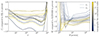 |
Fig. 3. Cosmic shear setup with the six KiDS-Legacy tomographic bins. The colour bar shows the tomographic bin index combination, I (i.e. for tomographic bins i, j the index is |

7.1. KiDS-Legacy
The final data release of KiDS (de Jong et al. 2013) and VIKING (VISTA Kilo-degree INfrared Galaxy, Edge et al. 2013) is described in detail in Wright et al. (2024) and is referred to as the fifth data release (dr5). Covering a survey area of 1347 deg2, it encompasses 9 photometric bands spanning from optical to near-infrared, with a 5σ limiting magnitude of 24.8 in the r-band. The footprint of the main survey includes a 4deg2 overlap with existing deep spectroscopic surveys. This data is complemented by an additional 23 deg2 KiDS- and VIKING-like imaging over additional deep spectroscopic fields, yielding a total of about 126 000 sources with both spectroscopy and photometry, crucial for robust redshift calibration (Wright et al. 2025a) across the dr5 footprint. Relative to the fourth data release (Kuijken et al. 2019), dr5 represents a roughly 30 per cent increase in area coverage and around 0.4 magnitude deepening in the i-band.
Significantly, the photometric redshift calibration has been refined, as outlined in Wright et al. (2025a). Notably, a new matching algorithm enables the generation of highly realistic mock catalogues for both photometric and spectroscopic sources. Redshift calibration employs two techniques: colour-based self-organising maps (SOM) and a clustering redshift-based approach, leveraging extensively the spectroscopic samples from dr5. The SOM method yields residual shifts in the mean redshift of each tomographic bin 〈δz〉≤0.01, serving as a conservative error floor on the priors for the mean redshifts of each bin. These enhancements, combined with the dr5 data, facilitate the calibration of an additional tomographic bin with redshift up to z≈2, resulting in a total of six bins compared to five in the previous CS analysis in KiDS-1000. The KiDS-Legacy is then a subsample of the whole galaxy catalogue with certain quality requirements, for example for the shape measurements, as well as selection criteria such as masking or blended sources. This leads to a final catalogue of around 4×10⁷ galaxies for CS over an effective area of roughly 1000 deg2.
7.2. KiDS-Legacy covariance
In this part, the covariance modelling choices in a KiDS-Legacy-like analysis as it will be carried out in Wright et al. (2025b) and Stölzner et al. (2025) are discussed. While the cosmology remains fixed to the fiducial values presented in Table 1 for all plots, it is important to note that for the actual cosmological analysis, an iterative approach is adopted for covariance calculation. Initially, a fiducial covariance matrix is utilised, followed by maximising of the posterior and iterative updates to the covariance. This iterative process, typically converges after one iteration, as shown in van Uitert et al. (2018), resulting in final contours that exhibit negligible changes, as demonstrated in the subsequent results.
Fiducial choice of cosmological parameters within ΛCDM used for the forward simulations to test the signal and noise modelling for KiDS-Legacy-like. The given cosmology is equivalent to S8≡σ8[(Ωb+Ωc)/0.3]1/2=0.82. The parameters are set in accordance with the constraints from KiDS-1000 (Asgari et al. 2021b), while σ8 is set to be the mid-value between KiDS-1000 and Planck (Planck Collaboration VI 2020).
In Figure 1 we show how the inference of S8 is affected by different modelling choices of the covariance for real space correlation functions and bandpowers (COSEBIs almost pick the same scales as bandpowers, so we do not show them here explicitly). The grey band corresponds to the 68 per cent interval together with the posterior maximum of the marginal distribution for the fiducial choice for the covariance modelling whose settings we are summarising in the following. We model the Gaussian term with an idealised mixed term (see Figure 5), but shape noise is estimated from the catalogue. The covariance always includes a multiplicative shear bias uncertainty, since it is not marginalised over in the inference process via sampling. We include the non-Gaussian covariance and the SSC term with a non-binary mask with the realistic survey footprint to calculate its variance. We use the standard NLA model in the covariance as discussed in Section 4, but stress again that the particular choice does not matter and that the code is flexible enough to deal with any alignment model on the Gaussian covariance level. Lastly, the matter power spectrum is modelled using hmcode2020 (Mead et al. 2020) with feedback controlled via log10TAGN. Each blue dot with error bars corresponds to an analysis where a specific attribute in the covariance modelling is varied.
Figure 1 shows the influence of individual modelling choices on the marginal constraints on S8 Nonetheless, it is important to acknowledge altering multiple fiducial assumptions about the covariance, e.g. ignoring the realistic pair counts, changing the IA model and removing the SSC contribution, could lead to a bias in the final value of S8. However, ignoring the non-Gaussian and SSC contribution on its own has very little effect on the constraints on S8. This is in particular reassuring for the non-Gaussian term, which is only accurate to 20 per cent (Joachimi et al. 2021). Especially the addition of the sixth tomographic bin in KiDS-Legacy compared to KiDS-1000 will make the nG contribution less pronounced as more linear scales with high signals are added to the analysis. Furthermore, due to the increase in effective area, the survey response is also smaller than in KiDS-1000.
Interestingly, we find that the use of the idealised pair counts (i.e. not using the pair counts from the catalogue but instead the analytic formula) has little effect on the S8 inference. This might be surprising at first, since using the analytic pair counts will change diagonal elements of the covariance matrix by up to 20 per cent (Troxel et al. 2018). However, we can explain this by the fact that the signal-to-noise ratio of the measurement in this case is almost unchanged. The reason for this is that changing the variance will also change the amount of correlation between the different data points. So if the analytic pair counts over (under) estimate the number of pairs, the variance in the fiducial setting will be larger (smaller), which makes the individual data point less significant for the inference. However, this effect also reduces (increases) correlations between the different data points, thus increasing the information content. Those two effects seem to balance each other such that the S8 constraints do not change. Interestingly, we also find that using a circular mask instead of the real footprint has the same effect as ignoring the SSC term altogether. IA seems to have a larger effect on real space correlation functions than on bandpowers which could be indicative of the fact that this is driven by contributions from large multipoles to ξ±. At the same time, however, we find that the case with no feedback changes both real space correlation functions and bandpowers in the same way. In general, we find the consistent trend that contributions decreasing the covariance will bias the constraint on S8 to larger values, as expected by signal-to-noise considerations. It should also be highlighted that, while the marginal posterior maximum can shift, the upper limit of the 68 per cent interval is very robust. Here we find the largest effect from the new mixed term (compare Figure 5 and Appendix F), since it strongly changes the off-diagonal elements of the covariance matrix while leaving the diagonals untouched. We note that we do not include the new mixed term in the COSEBIs or bandpower covariance matrix at this stage, since they are mapped directly from harmonic space and not from real space to avoid discretisation effects or the computation of a very finely sampled real space covariance matrix.
All those considerations are of course very specific to the KiDS-Legacy survey. They show, however, that our inference of S8 and in particular the upper limit of the corresponding error is very robust when changing the covariance modelling. While the impact of the mixed term seems very daunting in the light of next-generation surveys it should be highlighted that KiDS is a ground-based, single-visit survey, thus being much more inhomogeneous than Euclid or LSST, which are either in space or scan the same patch of the sky multiple times respectively. It is thus expected that the idealised mixed term is more accurate for these surveys.
In Figure 2, we scrutinise the different contributions of the covariance matrix for the KiDS-Legacy analysis, focusing on the COSEBIs covariance. Since we have shown ξ± and bandpowers so far, we discuss this using the COSEBIs covariance. Specifically, we plot the Pearson correlation coefficient. The structure of each of the six subplots is the following: the COSEBI mode, n, varies in each small square from n=1,…,5 while the tomographic bin combination i≤j, from one square to the next. We also do not show the covariance of the Bn modes, as they are only given by the shape noise contribution. Lastly, we only include cosmological contributions and do not consider the multiplicative shear bias uncertainty. The six large subsquares of Figure 2 show the six terms of the covariance matrix discussed in Section 2.1. The covariance is dominated completely by the Gaussian term, with the SSC and nG contribution only making up to around 35 and 15 per cent each on the off-diagonals. The Gaussian contribution itself is dominated by the sample variance terms on the off-diagonals, while the shape noise and the mixed term dominate the diagonals, with relative importance increasing towards tomographic bins at higher redshift.
7.3. Comparison with selected existing codes
The analytical covariance utilised in KiDS-1000 has undergone extensive testing against mock data, as detailed in Joachimi et al. (2021). While some of these tests are reiterated in the following sections using updated simulations, we present a selection of results to validate the OneCovariance code.
Given that the OneCovariance code interfaces with camb for linear and non-linear matter power spectra, and other codes like ccl employ a modified version of our halo model trispectrum implementation, we do not validate these quantities directly. The first step of our validation is therefore to compare the CS angular power spectra, or in other words, the line-of-sight projection. On the left side of Figure 3 we demonstrate the relative accuracy of the OneCovariance code compared to ccl. A KiDS-Legacy-like setup with six source bins was used and the non-linear matter power spectrum has been calculated using halofit (Takahashi et al. 2012). The tomographic bin combination index is colour-coded, that is labelling each bin combination, i≤j with a unique number starting at one. We find that the agreement is well below one per cent, except for the very first tomographic bin. This difference originates from slightly different extrapolations used for the non-linear matter power spectrum (as can be seen by the steep rise at large multiples) as well as the kind of interpolation used for the source redshift distributions. The small visible spikes are of order 10−3 and can be traced back to different accuracy settings when CAMB is called via ccl or the OneCovariance as well as slightly different interpolation schemes. However, we find excellent agreement with ccl.
Another critical validation step involves comparing our code with the covariance code used in the KiDS-1000 analysis. The right panel of Figure 3 displays the percentage difference between the OneCovariance code and the previously employed code for the diagonal elements of the ξ± covariance matrix, excluding shape noise. We conducted this comparison across nine logarithmically spaced angular bins ranging from 0.5 to 300 arcmin. Once again, we observe excellent agreement, with differences within a few per cent. Slightly larger disparities are noted at small angular scales, primarily attributed to differences in integration accuracy and cut-off limits for the integrals, particularly for the non-Gaussian (nG) and super-sample covariance (SSC) contributions. However, these discrepancies, while reaching up to 15 per cent, are not significant as small scales are shot-noise dominated, thereby minimally impacting previous analyses. Similar validation procedures were repeated for bandpowers and COSEBIs, yielding agreement below a per cent with previous studies (Joachimi et al. 2021; Asgari et al. 2021b). Notably, due to the more compact Fourier filters, the agreement for these cases is even better than for real space statistics. Additionally, we verified that we obtain identical results when passing Fourier filter functions externally to the code for different statistics (for how to pass external information, see Appendix A).
8. Validation against simulations
Testing the CS signal and noise modelling for the final release of the KiDS data, dr5, necessitates a substantial number of realisations of the data to accurately characterise the covariance. Achieving this requires forward simulations that closely resemble real data, incorporating factors such as the survey mask and variable depth. In this section, we detail the construction of the forward simulations employed to validate the error modelling in KiDS-Legacy. Section 8.1 provides an overview of the log-normal mocks and Section 8.2 briefly describes how the mocks are populated with galaxies and how the shape catalogues are created. Lastly, in Section 8.3 we compare the simulations against the analytical covariance.
Central to our assessment are key comparison figures that directly juxtapose our most realistic mock with the OneCovariance code. As all summary statistics can be derived from the real space correlation function, we only measure those on the mocks. Figures 4, 5, and 6 show the comparison for the signal, the correlation coefficient and diagonal covariance matrix elements respectively.
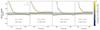 |
Fig. 4. Relative difference between the signal measured in the 4224 Egretta mocks (realistic mask and depth variations) with the signal prediction of OneCovariance code. The colour bar indicates the different unique tomographic bin combinations, the same as in Figure 3. The dashed lines show ξ− and solid lines ξ+. The grey band indicates a five per cent relative difference. The different plots show varying settings in the OneCovariance code. In particular, we distinguish whether the averaging over the θ bin (see Equation (61)) is carried out and if the pixel window due to the finite resolution of the healpix map is taken into account, i.e. damping power on small scales (Nside correction). |
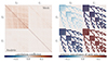 |
Fig. 5. KiDS-Legacy covariance matrix for real space correlation functions. Each square represents a unique combination of tomographic bins and contains the covariance for that combination in nine angular bins between 0.5 and 300 arcmin. The diagonals are in the order i≤j with the tomographic bin indices i and j. Left: correlation coefficient of the full covariance matrix without multiplicative shear bias uncertainty. In the lower triangle, the analytic covariance is shown, while the upper triangle shows the covariance as measured in the Egretta mocks (realistic mask and depth variations). Right: relative impact of the new mixed term (see Appendix F) on the Gaussian part covariance matrix compared to an idealised mixed term with a homogeneous pair and triplet counts. The latter were directly estimated from the KiDS-Legacy-like catalogue. |
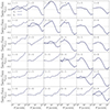 |
Fig. 6. Relative difference between the standard deviation of the Egretta mocks (realistic mask and depth variations) and that from the analytic covariance matrix from the OneCovariance code for the same setting as Figure 5. The dashed lines show ξ− and solid lines depict ξ+. The tomographic bin combination is shown in the top left corner of each subplot. |
8.1. GLASS simulations
The forward simulations for covariance validation in this study are founded on the KiDS-SBI14 suite of simulations detailed in von Wietersheim-Kramsta et al. (2025). At the core of the pipeline lie log-normal mocks of the 3-dimensional matter distribution in radial shells, which are subsequently projected along the line of sight to create shear maps. This process is facilitated within the GLASS15 (Generator for Large-Scale Structure) framework (Tessore et al. 2023). GLASS generates log-normal realisations to match the two-point statistics of the given input power spectrum. While higher-order statistics are not precisely recovered due to the inherently non-log-normal nature of the cosmic density field, this nonlinear transformation captures a significant portion of the trispectrum (Friedrich et al. 2021; Hall & Taylor 2022) relevant for the covariance matrix.
Within this framework, 4224 simulations are created for two distinct survey configurations, akin to the one selected in Joachimi et al. (2021), a discussion of which is provided in further detail in Section 8.2. The cosmological parameters remain fixed at the values specified in Table 1. The 3-dimensional power spectrum of the input matter is computed using camb (Lewis et al. 2000; Lewis & Bridle 2002; Howlett et al. 2012), with non-linear corrections computed from hmcode2020 (Mead et al. 2020). After computing the angular power spectra of the matter distribution in 22 shells of roughly equal thickness spanning the KiDS-Legacy redshift range, GLASS generates corresponding log-normal matter fields in each shell. The shell thickness ranges between 100 and 200 h−1Mpc, ensuring a reasonably accurate description of the matter field as log-normal (Hall & Taylor 2022; Piras et al. 2023), while also being sufficiently finely sampled to accurately capture the matter overdensity along the line of sight. The computationally intensive integration for the Cℓ in the matter shells is executed using Levin's method (Levin 1996; Zieser & Merkel 2016; Leonard et al. 2023). Subsequently, the concentric shells are integrated along the line of sight, weighted by the lensing efficiency function (refer to Tessore et al. 2023, for detailed information), resulting in a CS field realisation covering the entire sky. It is noteworthy that intrinsic alignments are not included in the covariance matrix validation. However, this omission does not compromise the validity of our tests, given that intrinsic alignment exerts minimal influence on the covariance matrix (see Figure 1) even if removing it completely and generally shares the same functional form as the lensing signal, thus being equally well accounted for.
8.2. KiDS-Legacy-like mocks
Given a realisation of the density and shear fields, galaxies are sampled within those, including systematic effects such as the survey footprint and the effect of variable depth on the redshift distribution and the shape noise with the help of SALMO (Speedy Acquisition for Lensing and Matter Observables, Joachimi et al. 2021).
To create a realistic number density of galaxies, we utilise organised randoms (ORs, introduced in Johnston et al. 2021). ORs employ self-organising-maps (SOMs, Kohonen 1982) to generate random samples that follow the spatial variability induced by a high-dimensional systematic space. SOMs are unsupervised neural network algorithms which are designed to map a high-dimensional data space onto a two-dimensional map while preserving topological features of the input data space. We define a systematic data vector including atmospheric seeing, sky background light, stellar number density, dust extinction and variations in the point-spread function. The SOM provides a map of Tiaogeng (TG, see Yan et al. 2025, for a detailed explanation) weights, wTG, as a function of pixel on the sky. The TG weights quantify the anisotropic selection function on the galaxy sample observed within KiDS as a function of the aforementioned observational systematics in a manner that is independent of the cosmological signal in the data. We found the TG weights to be a good indicator of the local seeing, atmospheric transparency and signal-to-noise, so it can be considered a good estimator of variable depth. In particular, the TG weights are uncorrelated with the r-band magnitude measurements of galaxies and their photometric redshift, while being highly correlated with the magnitude limit in the r-band which KiDS uses for shape measurements, the degree of background noise, and the PSF variations. Hence, wTG can robustly predict the local observational depth independently of the galaxy position and shape measurements. Next, we partition each of the six tomographic bins into ten equi-populated bins in wTG. For each  we independently recompute the effective number density, neff, and the total ellipticity dispersion σϵ, from the galaxy population. It is possible to linearly interpolate neff and σϵ as a function of wTG allowing the evaluations of both quantities at every pixel in the KiDS-Legacy-like footprint from the single spatial wTG map. We use a footprint of approximately 1000 deg2 with an Nside=1024.
The redshift calibration itself uses the following photometric bin boundaries: [0.1, 0.42, 0.58, 0.71, 0.9, 1.14, 2), adding a sixth tomographic bin in KiDS-Legacy compared to KiDS-1000 (see Section 7.1) By applying this binning scheme to the mock catalogues, we obtain the redshift distributions discussed above from the SOM, mapping the observed photometric redshifts to spectroscopic redshifts based on a reference spectroscopic sample (Wright et al. 2020; Hildebrandt et al. 2021).
Having set up the forward simulations, the two-point correlation functions ξ± are measured on each realisation using TreeCorr (Jarvis et al. 2004), following the same implementation described in Giblin et al. (2021), Joachimi et al. (2021). Initially, ξ± are measured in the north and south separately using 300 logarithmically spaced bins in θ∈[0.5, 300] arcmin. The estimated correlation functions,  are then combined as a weighted mean,
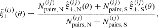 (89)
(89)
with the weighted galaxy pairs and measured correlation functions in tomographic bins i and j in the north (N) and south (S) fields respectively. Lastly, the finely binned correlation functions are then re-binned into the final nine logarithmically spaced θ bins covering the same range.
In Joachimi et al. (2021), three kinds of mocks, Buceros, Cygnus and Egretta, with increasing complexity were distinguished. Buceros is an idealised survey with a simple rectangular footprint and a homogeneous number density which serves as a baseline check of the covariance modelling, which was already found to agree within a few per cent with the analytical covariance (Joachimi et al. 2021). Given the agreement of the OneCovariance with the KiDS-1000 covariance matrix, see Figure 3, this mock as such is not considered. In case of Cygnus, we mask the simulations according to a realistic KiDS-Legacy-like mask. However, the survey is kept homogenous in neff and σϵ. In particular, the intrinsic ellipticities are sampled from a Gaussian distribution with fixed σϵ and zero mean for each tomographic bin. In the most complex mock, Egretta, the homogeneity and isotropy assumption in n(z), neff and σϵ are dropped, and they are sampled from realisations in the wTG maps. Therefore, Egretta is a realistic representation of the real KiDS-Legacy-like catalogue, including all systematics discussed before. It will therefore be used as the benchmark for the analytical covariance matrix. For more details on the simulations, we refer the reader to Joachimi et al. (2021).
8.3. Comparison with mocks
We limit the discussion to the most realistic mock, Egretta, since a general comparison between the different mock settings was already done in Joachimi et al. (2021) which the OneCovariance code was validated against. Having said that, we want to briefly summarise those results here again. For the Buceros mock with an idealised footprint and homogeneous survey properties, we find agreement and the percentage with slightly larger difference at large separations. Due to the more complex survey mask in Cygnus, those difference become more pronounced, leading to ten per cent differences at 300 arcmin separation. At smaller scales, however, the difference is still well below five per cent.
Before delving into the covariance comparison with Egretta we show the relative difference between the signal measured in the simulations for ξ± and calculated from theory via the OneCovariance code is shown in Figure 4. Dashed lines represent ξ− and solid lines ξ+ while the colour bar indicates the tomographic bin index combination. The four panels show different settings of the theory calculation. In particular, the resolution of the simulation is partially mimicked by taking the pixel window into account which dampens the power on scales, ℓ≤Nside and we explicitly average over angular bins in which the correlation function is measured. The grey band shows a 5 per cent difference between the simulation and the theory predictions. In general, we see good agreement between the theoretical predictions and the simulation, within 5 per cent. Incorporating the damping of small-scale power into the theoretical predictions slightly enhances the agreement on small angular scales. However, because of the broad filter function in Fourier space of ξ±, the small angular bins necessitate information from relatively small scales and are thus not accurately represented in the simulation. This effect is particularly noticeable for ξ− which requires integration up to ℓ>104 to reach convergence for θ<arcmin, although it is not evident for ξ+ at the scales displayed in this figure for clarity. For ξ+, this effect can be observed at scales below a few arcminutes. Nevertheless, for the covariance comparison, this limitation should not present a significant issue, as the covariance will be predominantly influenced by shape noise on small scales. Additionally, we observe that bin-averaging introduces differences of a few per cent across all angular bins, with no significant variation as a function of θ, consistent with expectations due to the logarithmic binning scheme.
On the left side of Figure 5, we present the covariance for the setup outlined in Section 8.2. The lower triangle displays the analytic prediction, while the upper triangle shows the covariance estimated from the mock data. Visually, there is excellent agreement between the simulation and theory for the correlation coefficient. The elements are ordered in such a way that each square corresponds to a unique combination of tomographic bins, arranged in increasing order such that i≤j. Overall, it is evident that the covariance is dominated by shape noise. However, for the tomographic bins at higher redshifts, as discussed in more detail in Section 7.2, other contributions become more pronounced.
The right panel of Figure 5 illustrates the impact of this modelling choice for the mixed term on the covariance matrix. Specifically, it shows the relative difference between these two cases for the Gaussian covariance matrix, i.e. considering an idealised mixed-term with homogeneous number density and no masking effects relative to using the triplet counts directly from the catalogue (compare Equation (6) and Appendix F respectively). Generally, we observe that the effect is most pronounced at large or small angular separations, while intermediate separations are less affected. This behaviour is expected because large scales are influenced by the extent of the survey, while very small scales can be affected by masking effects within the survey area. Additionally, the effect on the diagonal is less noticeable due to the contribution of shape noise.
For ξ+, the effect of the updated mixed term reaches a maximum of 10 per cent. However, for ξ− and its cross-correlation with ξ+, the effect can be significant for individual elements of the covariance matrix, exceeding 50 per cent. Nonetheless, since the signal strength for ξ− is relatively small, this effect is mitigated by the shape noise (its impact on inference is discussed in Section 7.2). It is worth noting that although there are individual points showing a substantial effect in the cross-covariance between ξ+ and ξ−, this is attributed to numerical noise and does not influence the results since the corresponding covariance matrix elements are very small.
We anticipate this effect to be less pronounced for larger and more homogeneous surveys than KiDS-Legacy. Surveys like Euclid and LSST are expected to have fewer spatial variations in the number density of sources. This statement, however, bears the caveat that the other components of the covariance matrix will become more significant for these surveys as they are deeper, resulting in a stronger CS signal compared to the shape noise. Therefore, a concluding analysis of the impact of the mixed term in a stage 4 survey will be the subject of future work.
Finally, Figure 6 illustrates the relative difference in the standard deviation, i.e. the square root of the diagonal elements of the covariance matrix, between Egretta and the OneCovariance code. There is excellent agreement at small angular scales due to the contribution of shape noise, as the pair counts are matched to those measured in the Egretta mocks. It is worth noting that we address the most significant effect of variable depth, which generally changes the shape-noise in KiDS-Legacy compared to a uniform galaxy distribution. This effect is driven by the distribution of wTG, which skews above the mean, resulting in most pixels in the field being under-dense compared to the mean galaxy density. Generally, the agreement between the mocks and the analytical covariance is of a slightly better level than in previous analysis (Joachimi et al. 2021). Due to the increased sensitivity of KiDS-Legacy compared to KiDS-1000 the question arises whether this agreement is good enough. As discussed above, the main effect is the survey geometry which we address in Appendix F reconsideration of the mix term and via the pair counts in Equation (64). In the ‘sva’ term, however, the survey geometry is only accounted for via the fsky approximation. To asses the accuracy we analysed mock data vectors with the fiducial KiDS-Legacy covariance (compare to the grey band in Figure 1), including the new mixed term, and directly with Egretta. We found that using the Egretta covariance gives a shift in χ2 similar to the inclusion of the survey geometry in the mix term. From this we conclude that the fsky approximation in the ‘sva’ term is still accurate enough for KiDS-Legacy. If the sensitivity with upcoming surveys is further increased, this approximation might need to be reconsidered. This point is discussed a bit more in the conclusions.
9. OneCovariance applications
To demonstrate the versatility of the OneCovariance code, we employ it to address two additional key aspects of the KiDS-Legacy analysis: consistency tests among different summary statistics in Section 9.1 and clustering redshifts in Section 9.2. These aspects are integral to the studies presented in Stölzner et al. (2025) and Wright et al. (2025b), respectively. In Figure 7, we present the correlation coefficient between the three main summary statistics utilised in KiDS-Legacy. For the clustering redshift covariance, our primary findings are depicted in Figures 8 and 10. These illustrations offer a comparison with mocks and validate the fundamental structure of the jackknife covariance employed for the redshift calibration.
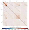 |
Fig. 7. Showcase of the consistency tests possible with the OneCovariance code. This is a cosmic shear setting as in KiDS-1000 (Asgari et al. 2021b) (i.e. five tomographic bins, eight band power bins, five modes for COSEBIs, and nine bins for ξ±. The code was used to create the full covariance matrix for any pair of those three statistics. Since these are all summary statistics for the same tracer and almost over the same physical scales, the matrix is close to being singular. The full matrix shown here has a single negative eigenvalue originating from numerical noise. However, the subcovariance matrices between each pair of summary statistics are still positive-definite. We do not show the B modes for COSEBIs and bandpowers since they mainly consist of shape noise (although they are still highly correlated with the shape noise of the other statistics). |
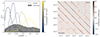 |
Fig. 8. Left: redshift distribution of the target sample for five tomographic bins of KiDS-1000 as solid lines. The grey bars indicate the reference sample. Right: Pearson correlation coefficient with the lower triangle showing the predictions of the analytical prescription, Equation (91), while the upper triangle shows the results obtained by jackknife resampling from Hildebrandt et al. (2021) (compare their Figure 3). |
9.1. Consistency tests
As an initial showcase of the OneCovariance code's capabilities for KiDS-Legacy CS, we present the covariance matrix between various summary statistics. This calculation, facilitated by the ARBsummary class of the code (see Appendix A), serves as a foundational component for the consistency checks (or cross-validation) that will be carried out in Stölzner et al. (2025), a process that hinges not only on calculating the covariance of each summary statistic but also on their cross-covariance. Given that the different summary statistics probe nearly identical physical scales, the resulting covariance matrix exhibits significant cross-correlation and can be close to singular.
As a specific example and to demonstrate the versatility of the OneCovariance code, we undertake the covariance matrix calculation for a KiDS-1000 setup. This pairwise computation encompasses our principal CS summary statistics. It is, however, available for arbitrary summary statistics of all tracers supported by the code.
The resulting correlation coefficient is depicted in Figure 7, showing large off-diagonal elements between different summary statistics originating both from sample variance terms as well as shape noise. Moreover, the pronounced correlations highlight that the diverse summary statistics employed in the KiDS-Legacy analysis are almost completely degenerate.
The OneCovariance code can straightforwardly accommodate any combination of summary statistics envisioned by the user since it propagates the relation between summary statistics and the harmonic covariance through simple integral transformations (compare Equation (51)). Consequently, users can seamlessly integrate different summary statistics for various tracers or explore the impact of different scale cuts for any summary statistic, as done for COSEBIs in Dark Energy Survey and Kilo-Degree Survey Collaboration (2023).
9.2. Clustering redshifts
As the final application of the OneCovariance code in this study, we investigate the covariance matrix of clustering redshift estimation (see e.g. Lima et al. 2008; Bonnett et al. 2016; van den Busch et al. 2020; Hildebrandt et al. 2021) which utilises a spectroscopic reference sample (s) and a target sample with noisy redshift estimates (p). In Hildebrandt et al. (2021) a covariance using jackknife resampling was used. So far, however, it was never compared to analytical expectation. In this section we are filling this gap. By measuring the correlation function, Equation (59), between these two samples at fixed physical scale r at different redshifts, the redshift distribution n(z) can be recovered up to an irrelevant multiplicative constant (as the redshift distribution will be normalised in the end) and bias evolution of the target sample,
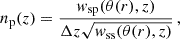 (90)
(90)
where Δz is the redshift width of each cross-correlation measurement. By labelling tomographic bin indices of the target sample with Greek letters and reference sample redshift bins with Latin letters, the covariance for this estimator at first order is
![Mathematical equation: $$ \begin{aligned} \mathrm {Cov}\left [n_\alpha ({z_i}),n_\beta ({z_j})\right ] &\equiv \mathrm {Cov}\left [\frac {{{\mathit {w}}}_{i\alpha }}{\Delta z_i\sqrt {{{\mathit {w}}}_{ii}}}\frac {{{\mathit {w}}}_{j\beta }}{\Delta z_j \sqrt {{{\mathit {w}}}_{jj}}}\right ] \\ &\approx \frac {1}{\Delta z_i \Delta z_j\sqrt {{{\mathit {w}}}_{ii}{{\mathit {w}}}_{jj}}}\left [C_{i\alpha j \beta } - \frac {{{\mathit {w}}}_{i\alpha }}{2{{\mathit {w}}}_{ii}}C_{iij\beta } - \frac {{{\mathit {w}}}_{j\beta }}{2{{\mathit {w}}}_{jj}}C_{i\alpha jj} + \frac {{{\mathit {w}}}_{i\alpha }{{\mathit {w}}}_{j\beta }}{4{{\mathit {w}}}_{ii}{{\mathit {w}}}_{jj}}C_{iijj}\right ]\,. \end{aligned} $$](/articles/aa/full_html/2025/07/aa52592-24/aa52592-24-eq149.gif) (91)
(91)
Here Cijkm denotes the covariance between clustering measurement wij and wkm at fixed scale r. The last three terms are only non-zero if i=j, with some small off-diagonal elements from the full non-Limber expression. Only the first term can have important off-diagonal elements, in particular where the redshift of the reference sample i approaches the support of the target sample β (and the same for j and α).
The performance evaluation of the analytic covariance for clustering redshifts is conducted using the synthetic data outlined in Hildebrandt et al. (2021) and van den Busch et al. (2020). This dataset comprises mock galaxy samples closely resembling the KiDS+VIKING-450 (KV450) CS sample. The basis of these mock samples is the MICE simulation (Fosalba et al. 2015). The cosmological model adopted in these simulations adheres to a ΛCDM model with parameters: Ωm=0.25, ΩΛ=1−Ωm, Ωb=0.044, σ8=0.8, and h=0.7. These simulations are accompanied by the corresponding galaxy catalogues (Crocce et al. 2015), serving as the foundation for the publicly accessible pipeline for generating KiDS mock samples16. Due to the nature of the estimator, the covariance retains a residual dependence on the bias evolution of the target sample. Davis et al. (2018) characterised this bias using the parametrisation ℬα(z)=(1+z)α, we use the values from van den Busch et al. (2020), Hildebrandt et al. (2021) for the residual bias evaluation in the covariance modelling.
Figure 8 illustrates the resulting redshift distributions for the five tomographic bins of KiDS1000, represented by solid colour-coded lines on the left side, denoting the target sample. The redshift distribution of the reference sample is depicted as a bar chart. On the right, the Pearson correlation coefficient of the corresponding covariance matrix is displayed for scales r∈[0.1,1] h−1 Mpc. In the upper triangle, we show the analytic prediction of Equation (91), while the lower triangle uses the mock catalogue and jackknife re-sampling over the individual subsamples of the simulation. The general structure is very similar, in particular, one can see that the previously mentioned non-vanishing off-diagonals at i≠j are in the correct position. Moreover, the diagonal of each block matrix exhibits comparable structures, providing valuable qualitative validation of the jackknife covariance outlined in Hildebrandt et al. (2021).
With the narrow redshift bins employed in cross-correlation measurements with spectroscopic surveys, the applicability range of the Limber approximation, as denoted by Equation (10), is significantly constrained. As discussed in Loverde & Afshordi (2008), the next-to-leading order term in the expansion becomes subdominant for ℓ>χ/Δχ, where Δχ is the width of a Gaussian redshift bin at co-moving distance χ. For the present situation, this requires the non-Limber calculation up to ℓ∼103. In the left plot of Figure 9, we depict the angular power spectrum of spectroscopic sample auto-correlations. Dashed lines represent the complete integral, as described in Equation (8), while solid lines utilise the Limber approximation. All lines are colour-coded with respect to the spectroscopic redshift bins (as illustrated in the bar plot of Figure 8). It is evident from the figure that the non-Limber projection significantly impacts the integrand of  . On the right side of Figure 9, we illustrate the impact of the non-Limber approximation on the Gaussian error of the covariance, revealing approximately 50 per cent effects for all tomographic bins.
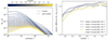 |
Fig. 9. Left: auto-correlation angular power spectra of the reference sample as a function of spectroscopic redshift (colour bar). The solid lines use the Limber approximation, Equation (10), while the dashed lines make use of the full expression, Equation (8). Right: fractional difference as a percentage of the Gaussian covariance term when using Limber vs non-Limber. |
Figure 10 presents, on the left side, the contributions to the covariance as a function of redshift, colour-coded according to the tomographic bin index. It is evident that low redshifts are significantly influenced by the non-Gaussian covariance (as indicated by dashed lines), while the shot noise contribution remains negligible for all redshifts. On the right side of Figure 10, we juxtapose the analytical covariance with simulations (indicated by symbols with thin lines). We observe a good agreement for the lower tomographic bins, with the increase attributed to the non-Gaussian contribution clearly visible. However, this increase is less pronounced in the fourth and fifth tomographic bins for the analytical covariance, whereas it remains evident in the mock data. This difference is likely due to uncertainties in the non-linear modelling of the trispectrum, especially as we measure signals deep within the non-linear regime, k>1h/Mpc.
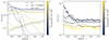 |
Fig. 10. Left: contribution to the standard deviation of the clustering redshift measurements. The solid lines correspond to the total variance, the dashed lines to the non-Gaussian contribution, and the dotted lines to the shot noise. For all tests, we ignored the SSC term since it is suppressed for galaxy clustering. Right: comparison of the analytical standard deviation (solid lines) with the simulations (symbols). |
It is worth noting that while the non-Limber effect is easily detectable for the Gaussian covariance, its influence on the non-Gaussian term presents a more challenging task and has thus far only been explored in Lee & Dvorkin (2020) for trispectra using specific kernels from perturbation theory and the galaxy bias expansion. Their analysis suggests significant effects on the trispectrum. However, a similar analysis for general trispectra, such as those from the halo model, remains unexplored and is beyond the scope of this section for several reasons. Firstly, while the OneCovariance can compute the non-Limber projection of power spectra, its primary utility lies in photometric surveys with broader window functions, where Limber's approximation is more readily applicable. Secondly, spectroscopic samples, necessitating non-Limber calculations, are typically conducted on quasi-linear scales, unlike the one presented here. On those scales, the non-Gaussian contribution is generally less significant. Lastly, this application serves as a comprehensive test and sanity check for clustering redshift covariance, where jackknife resampling is readily available. Furthermore, realistic samples are likely to be more influenced by noise, as galaxy density tends to be substantially lower, at least by a factor of ten.
10. Present and future of the OneCovariance code
In this section, we offer a summary of the capabilities of the code, delineate the modelling choices incorporated, underscore its flexibility, and contemplate potential avenues for future enhancements.
10.1. Current status of OneCovariance code
We have provided a comprehensive review of the covariance matrix modelling in KiDS so far in Sections 3 and 4. Employing a halo model approach, we have consolidated all relevant equations used in various analyses, encompassing CS (Hildebrandt et al. 2020; Asgari et al. 2021b), GGL, GC, and the CSMF (Heymans et al. 2021; Dvornik et al. 2018, 2023). This effort culminates in establishing the legacy of analytic covariance modelling within KiDS. While our primary focus lies on CS for the direct validation of the code in this study, we have implemented all pertinent quantities into the new OneCovariance code from scratch and cross-validated them against previous results. Moreover, we have reviewed and incorporated all summary statistics utilised within KiDS in Section 5, encompassing real space correlation functions, COSEBIs, and bandpowers, each applicable across all three tracers. Through the development of a unified code for covariance matrices, we have streamlined the calculation process, now directly linking harmonic space statistics to observables via integral transformations. This approach differs from that of KiDS-1000, where the bandpowers covariance was derived from the ξ± covariance. This modification brings the analytic covariance for bandpowers closer to the theoretical modules employed in KiDS, enhancing the consistency and efficiency of our analyses.
The OneCovariance offers users the capability to effortlessly download and compute simulation-validated covariance matrices for different traces across various statistical representations including harmonic space, real space, COSEBIs, and bandpowers, all under the flat sky approximation. While we focused on the comparison using CS in this paper, the code has been validated against all previous covariance codes employed in KiDS also for the other tracers. Minimal user input is required beyond specifying the redshift distributions, as the code operates out of the box. Moreover, the code's flexibility allows for extensive customisation. Users can readily adjust inputs, such as modifying the HOD prescription or directly altering galaxy power spectra or bias parameters. Additionally, it offers the flexibility to alter line-of-sight weight functions through input, facilitating the definition of entirely new tracers. For instance, by defining a new line-of-sight weight function and adjusting the HOD prescription, the code can compute the covariance matrix for the Cosmic Infrared Background or any other intensity mapping quantity. Alternatively, users can provide harmonic-space quantities directly, allowing the code to perform the necessary projections to observables. Furthermore, the code includes scripts to compute the weight functions used for various summary statistics in KiDS-Legacy.
The overarching philosophy of the OneCovariance code is centred on the replaceability of all essential quantities by file inputs. If a file input is provided, it supersedes the standard configuration of the code, utilising the file input instead. This approach permeates the entirety of the code, from fundamental quantities required for theory calculations, such as line-of-sight weights and bias prescriptions, to higher-level quantities including power spectra, their responses, and trispectra. The final elements of the covariance are effectively arrays for each tracer combination with the general shape

Here,  labels the spatial index of the tracer pair t1,t2 over which its two-point function is measured. This can be for example the θ bin, the band power mode, the order of the COSEBIs, or any other label of an arbitrary summary statistic passed to the code.
  is the corresponding stellar mass bin (this could be also modified to cluster number counts, for example). For CS, this always has a length of one. Lastly,
  and
and  is the tomographic bin combination for the pair (t1,t2). With this structured approach, the OneCovariance code possesses the versatility required to handle various scenarios in cosmology, allowing users to specify inputs via file paths in a configuration file. This means that users can specify the necessary inputs, thereby solving the often cumbersome task of ordering covariance matrix elements and performing the projection to observables. In essence, the OneCovariance code provides a comprehensive solution for covariance estimation whenever a HOD prescription-based halo model is employed for the signal, offering a valuable resource for the cosmological community.
10.2. Future developments of the code
The future development roadmap for the OneCovariance code includes both incremental improvements and significant expansions to its functionality. Here is an outline of the planned enhancements:
-
i)
Currently, the code employs the flat sky approximation for defining observables. In the next version, full sky transformations will be implemented, especially for the Gaussian terms, as they dominate the covariance on scales where curved sky effects become significant.
-
ii)
The code already supports calculating the non-Limber covariance for Gaussian contributions. The next step involves extending this capability to cover connected terms as well, enhancing the accuracy of covariance estimates.
-
iii)
Incorporating survey window effects into the harmonic space covariance and propagating them to observables, particularly for sample variance, will be a crucial addition to enhancing the accuracy of covariance estimates. This could be done by streamlining the code with NaMaster (Alonso et al. 2019).
-
iv)
A longer list of pre-implemented models will be added to reduce the number of required input quantities, including alternative HOD and bias prescriptions, streamlining the user experience and expanding the code's usability.
-
v)
Interfacing CCL (Chisari et al. 2019a) will be implemented, enabling the use of pre-defined quantities within CCL and leveraging its extensive functionalities for enhanced accuracy and efficiency in covariance calculations.
11. Conclusion
In this study, we have provided a comprehensive account of the covariance methodology utilised in and up to the latest data release of KiDS. This encompasses the validation of the CS covariance matrix utilised in Wright et al. (2025b) and Stölzner et al. (2025), as well as its application to clustering redshifts as employed in Wright et al. (2025a). Accompanying this paper is the OneCovariance code, a unified covariance tool tailored for photometric LSS surveys. We have conducted a thorough validation of the OneCovariance code for analysing KiDS-Legacy data, with a specific focus on CS. Our validation efforts have yielded several noteworthy conclusions. We have demonstrated that the theoretical predictions generated by the OneCovariance code align closely with those obtained from external libraries, such as ccl, at the per cent level. This underscores the robustness and accuracy of the code's theoretical predictions. Furthermore, comparisons with the independent implementation of the covariance matrix calculations from KiDS-1000, as detailed in Joachimi et al. (2021), being typically at the per cent level, reinforces the accuracy of the OneCovariance code. Any larger discrepancies identified were traced back to differences in accuracy settings or extrapolation schemes used for integrations when transitioning from harmonic space to observables. Importantly, we have verified that these discrepancies would not have significantly impacted any previous analyses conducted on the KiDS data. This ensures the consistency and reliability of previous findings derived from KiDS data analyses.
Our validation efforts provide strong evidence supporting the efficacy and accuracy of the OneCovariance code for CS analyses within the KiDS framework. This instils confidence in the code's utility for future cosmological investigations, ensuring robust and reliable covariance estimation in the analysis of LSS data. Next, we established a simulation pipeline to further validate the covariance matrix. We used log-normal realisations of the density field with both a realistic mask and homogeneous sources (Cygnus), as well as variations in source density (Egretta). On these mocks, we measured the real space correlation functions of the shear, ξ±, and found excellent agreement between the theoretical signal and the signal measured in the mocks. This agreement was observed across nine logarithmically spaced angular bins ranging from 0.5 to 300 arcmin. By leveraging the exact pair counts from the Egretta mocks, we also found similar agreement between the simulation and the analytic covariance as in KiDS-1000. Particularly, we observed agreement well within ten per cent on most scales, with only the largest angular scales exhibiting more significant deviations due to survey boundary effects. Importantly, these differences do not significantly impact the final constraints derived from the analysis.
A significant deviation from KiDS-1000 was the re-evaluation of the mixed term, namely the cross-correlation between shape noise and two-point statistics. This term is influenced by both the response of the signal to the survey geometry and the number of pairs used to estimate the signal itself, owing to the complex survey mask of KiDS. We found that assuming a homogeneous survey misestimates the Gaussian term by roughly 10 per cent in the case of ξ+ for off-diagonal elements, with this effect potentially being both positive and negative. For ξ− and its cross-correlation with ξ+, the deviation can be substantial on off-diagonal elements. This is attributed to the broad support of the Fourier filter for ξ− and its sensitivity to many scales, thus being affected by the inhomogeneity of the KiDS-Legacy sample and the intricate survey footprint. However, despite the potentially large effects on individual covariance matrix elements, the low signal of ξ− and high shape noise mitigate these discrepancies. For upcoming surveys, the situation is less clear. On the one hand, shape noise effects will become less important and the surveys will become more homogeneous as well as larger, reducing the importance of edge effects and variable depth. On the other hand, however, due to the increasing importance of sample variance and the increased overall sensitivity, the usage of an ideal mixed term might still lead to more significant effects on parameter inference. In future work, we plan an investigation of this issue along with the inclusion of the survey geometry in the ‘sva’ term. This can be done by using the pseudo-Cℓ covariance directly to incorporate the effect of the mask.
We examined the influence of various modelling choices for the covariance on the final inference of S8, demonstrating their robustness. These choices included the baryonic feedback prescription, the Super Sample Covariance (SSC) and non-Gaussian (nG) terms, the updated mixed term, and the intrinsic alignment model, among others. The upper bound of the 68 per cent interval of S8 remained largely unaffected by these modelling choices. Furthermore, we compared the impact of different terms on the covariance matrix and found that the Gaussian term overwhelmingly dominated on almost all scales and tomographic bins. The non-Gaussian and SSC contributions were of minor importance, with the SSC term slightly more significant across tomographic bins. One contributing factor to the diminished impact of these terms in KiDS-Legacy is the inclusion of the sixth tomographic bin, which enhances sensitivity to more linear scales, especially given the substantial CS signal in the sixth bin.
Furthermore, we demonstrated that the OneCovariance code can serve as a valuable tool for conducting consistency tests between different summary statistics or different surveys. That is, we calculate the covariance matrix for the same tracer (CS in this case), but two different summary statistics. We confirmed that the covariance matrices required for the KiDS-Legacy consistency tests (Stölzner et al. 2025) are invertible and well-behaved for pairs of summary statistics. This functionality holds significant importance when performing consistency tests between large-scale and small-scale analyses of CS data, particularly in addressing tensions such as the S8 tension. By enabling such tests, the OneCovariance code enhances the capability to probe and validate cosmological models across different scales and datasets.
In our final application of the OneCovariance code, we turn our attention to the estimation of the covariance matrix for clustering redshifts, a critical component utilised in Wright et al. (2025b) to validate the jackknife covariance employed for n(z) calibration. Our approach involved applying the code to a KiDS-1000 redshift distribution, slated for calibration against an idealised reference sample derived from the MICE2 simulations, approximately ten times denser than the actual dataset. Our analysis revealed encouraging results; there was a generally good agreement observed for the correlation coefficient between the analytical and jackknife covariance derived directly from the mocks. However, the narrow redshift shells over which the signal is averaged at a given physical scale posed a challenge, rendering the Limber expression inapplicable over a broad range of scales. Consequently, the covariance experienced deviations of up to 50 per cent. To address this issue, we incorporated the full non-Limber expression in the Gaussian covariance, while assuming the Limber expression for the non-Gaussian component. However, we recognise that a comprehensive treatment necessitates a full non-Limber modelling of the non-Gaussian covariance, a task beyond the scope of this paper. Nevertheless, our analytical covariance matrix effectively captured the salient features of the jackknife covariance, thereby serving as a valuable cross-check for the clustering redshift calibration process.
In summary, our study confirms the robustness of the KiDS-Legacy covariance in delivering accurate results for the S8 parameter. By providing the cosmological community with a versatile tool capable of calculating covariance matrices for a wide array of photometric(-like) LSS observables in both current and future surveys, we hope to facilitate further advancements in cosmological research.
Acknowledgments
The authors would like to thank an anonymous referee for valuable comments. RR, AD, JLvdB, HH and CM are supported by a European Research Council Consolidator Grant (No. 770935). SU, BS and ZY acknowledges support from the Max Planck Society and the Alexander von Humboldt Foundation in the framework of the Max Planck-Humboldt Research Award endowed by the Federal Ministry of Education and Research. HH is supported by a DFG Heisenberg grant (Hi 1495/5-1), the DFG Collaborative Research Center SFB1491 and the DLR project 50QE2305. BJ acknowledges support from the ERC-selected UKRI Frontier Research Grant EP/Y03015X/1 and by STFC Consolidated Grant ST/V000780/1. MA is supported by the UK Science and Technology Facilities Council (STFC) under grant number ST/Y002652/1 and the Royal Society under grant numbers RGSR2222268 and ICAR1231094. MvWK acknowledges the support by the Science and Technology Facilities Council. AHW is supported by the Deutsches Zentrum für Luft- und Raumfahrt (DLR), made possible by the Bundesministerium für Wirtschaft und Klimaschutz, and acknowledges funding from the German Science Foundation DFG, via the Collaborative Research Center SFB1491 ‘Cosmic Interacting Matters – From Source to Signal’. MB and PJ are supported by the Polish National Science Center through grant no. 2020/38/E/ST9/00395. MB is supported by the Polish National Science Center through grants no. 2018/30/E/ST9/00698, 2018/31/G/ST9/03388 and 2020/39/B/ST9/03494. PB acknowledges financial support from the Canadian Space Agency (Grant No. 23EXPROSS1) and the Waterloo Centre for Astrophysics. JHD acknowledges support from an STFC Ernest Rutherford Fellowship (project reference ST/S004858/1). CG acknowledges support from the project ‘A rising tide: Galaxy intrinsic alignments as a new probe of cosmology and galaxy evolution’ (with project number 1393VI.Vidi.203.011) of the Talent programme Vidi which is (partly) financed by the Dutch Research Council (NWO). SJ acknowledges the Dennis Sciama Fellowship at the University of Portsmouth and the Ramón y Cajal Fellowship from the Spanish Ministry of Science. KK acknowledges support from the Royal Society and Imperial College. LL is supported by the Austrian Science Fund (FWF) [ESP 357-N]. CM acknowledges support under the grant number PID2021-128338NB-I00 from the Spanish Ministry of Science. TT acknowledges funding from the Swiss National Science Foundation under the Ambizione project PZ00P2_193352 MY acknowledges funding from the European Research Council (ERC) under the European Union's Horizon 2020 research and innovation program (Grant agreement No. 101053992). Software: The figures in this work were created with matplotlib (Hunter 2007), making use of the NumPy (Harris et al. 2020), SciPy (Virtanen et al. 2020), Cosmosis (Zuntz et al. 2015), Nautilus (Lange 2023) and CosmoPower (Spurio Mancini et al. 2022) software packages. Author contributions: All authors contributed to the development and writing of this paper. The authorship list is given in three groups: the lead authors (RR, SU) followed by two alphabetical groups. The first alphabetical group includes those who are key contributors to both the scientific analysis and the data products. The second group covers those who have either made a significant contribution to the data products, or to the scientific analysis.
Ψ-stats are the COSEBIs-equivalent for GGL and GC equivalent.
It should be noted that the vanilla halo model requires some more attention to accurately fit the transition region between the one-halo and two-halo term. Furthermore, for higher-order statistics these tweaks become more involved (see Takahashi et al. 2020 for the bispectrum). However, for the trispectrum contribution to the covariance, the accuracy of the halo model is, at least currently, sufficient.
We refer to the natural logarithm as ln(x) and to the logarithm to base ten as log(x).
Available on https://github.com/rreischke/OneCovariance
Accessible at https://github.com/KiDS-WL/MICE2_mocks
Ten because it includes B modes for lensing. Instead, for pure Cℓ, there are only six.
For ensuring a higher accuracy one could also divide the θi into sub-intervals which are then put into the corresponding  combination.
References
- Abbott, T. M. C., Abdalla, F. B., Alarcon, A., et al. 2018, Phys. Rev. D, 98, 043526 [NASA ADS] [CrossRef] [Google Scholar]
- Abbott, T. M. C., Aguena, M., Alarcon, A., et al. 2022, Phys. Rev. D, 105, 023520 [CrossRef] [Google Scholar]
- Alonso, D., Sanchez, J., Slosar, A., & LSST Dark Energy Science Collaboration 2019, MNRAS, 484, 4127 [NASA ADS] [CrossRef] [Google Scholar]
- Amon, A., Gruen, D., Troxel, M. A., et al. 2022, Phys. Rev. D, 105, 023514 [NASA ADS] [CrossRef] [Google Scholar]
- Angulo, R. E., Zennaro, M., Contreras, S., et al. 2021, MNRAS, 507, 5869 [NASA ADS] [CrossRef] [Google Scholar]
- Aricò, G., Angulo, R. E., Contreras, S., et al. 2021, MNRAS, 506, 4070 [CrossRef] [Google Scholar]
- Asgari, M., & Schneider, P. 2015, A&A, 578, A50 [NASA ADS] [CrossRef] [EDP Sciences] [Google Scholar]
- Asgari, M., Heymans, C., Hildebrandt, H., et al. 2019, A&A, 624, A134 [NASA ADS] [CrossRef] [EDP Sciences] [Google Scholar]
- Asgari, M., Friswell, I., Yoon, M., et al. 2021a, MNRAS, 501, 3003 [NASA ADS] [CrossRef] [Google Scholar]
- Asgari, M., Lin, C. -A., Joachimi, B., et al. 2021b, A&A, 645, A104 [NASA ADS] [CrossRef] [EDP Sciences] [Google Scholar]
- Asgari, M., Mead, A. J., & Heymans, C. 2023, Open J. Astrophys., 6, 39 [NASA ADS] [CrossRef] [Google Scholar]
- Astropy Collaboration (Price-Whelan, A. M., et al.) 2022, ApJ, 935, 167 [NASA ADS] [CrossRef] [Google Scholar]
- Barreira, A., Krause, E., & Schmidt, F. 2018, J. Cosmol. Astropart. Phys., 2018, 015 [Google Scholar]
- Bartelmann, M., & Schneider, P. 2001, Phys. Rep., 340, 291 [Google Scholar]
- Bartelmann, M., Dombrowski, J., Konrad, S., et al. 2021, SciPost Phys., 10, 153 [Google Scholar]
- Becker, M. R., Troxel, M. A., MacCrann, N., et al. 2016, Phys. Rev. D, 94, 022002 [NASA ADS] [CrossRef] [Google Scholar]
- Bernardeau, F., Colombi, S., Gaztañaga, E., & Scoccimarro, R. 2002, Phys. Rep., 367, 1 [Google Scholar]
- Bernardeau, F., Nishimichi, T., & Taruya, A. 2014, MNRAS, 445, 1526 [Google Scholar]
- Blas, D., Lesgourgues, J., & Tram, T. 2011, JCAP, 07, 034 [CrossRef] [Google Scholar]
- Blazek, J. A., MacCrann, N., Troxel, M. A., & Fang, X. 2019, Phys. Rev. D, 100, 103506 [NASA ADS] [CrossRef] [Google Scholar]
- Bonnett, C., Troxel, M. A., Hartley, W., et al. 2016, Phys. Rev. D, 94, 042005 [Google Scholar]
- Bridle, S., & King, L. 2007, New J. Phys., 9, 444 [Google Scholar]
- Buddendiek, A., Schneider, P., Hildebrandt, H., et al. 2016, MNRAS, 456, 3886 [Google Scholar]
- Cacciato, M., van den Bosch, F. C., More, S., et al. 2009, MNRAS, 394, 929 [NASA ADS] [CrossRef] [Google Scholar]
- Cacciato, M., van den Bosch, F. C., More, S., Mo, H., & Yang, X. 2013, MNRAS, 430, 767 [Google Scholar]
- Carrasco, J. J. M., Hertzberg, M. P., & Senatore, L. 2012, JHEP, 2012, 82 [Google Scholar]
- Castro, P. G., Heavens, A. F., & Kitching, T. D. 2005, Phys. Rev. D, 72, 023516 [NASA ADS] [CrossRef] [Google Scholar]
- Chisari, N. E., & Pontzen, A. 2019, Phys. Rev. D, 100, 023543 [Google Scholar]
- Chisari, N. E., Alonso, D., Krause, E., et al. 2019a, ApJS, 242, 2 [Google Scholar]
- Chisari, N. E., Mead, A. J., Joudaki, S., et al. 2019b, Open J. Astrophys., 2, 4 [NASA ADS] [CrossRef] [Google Scholar]
- Cooray, A., & Hu, W. 2001, ApJ, 554, 56 [Google Scholar]
- Cooray, A., & Sheth, R. 2002, Phys. Rep., 372, 1 [Google Scholar]
- Crocce, M., Castander, F. J., Gaztañaga, E., Fosalba, P., & Carretero, J. 2015, MNRAS, 453, 1513 [NASA ADS] [CrossRef] [Google Scholar]
- Dalal, R., Li, X., Nicola, A., et al. 2023, Phys. Rev. D, 108, 123519 [CrossRef] [Google Scholar]
- Dark Energy Survey and Kilo-Degree Survey Collaboration (Abbott, T. M. C., et al.) 2023, Open J. Astrophys., 6, 36 [NASA ADS] [Google Scholar]
- Davis, C., Rozo, E., Roodman, A., et al. 2018, MNRAS, 477, 2196 [Google Scholar]
- de Jong, J. T. A., Verdoes Kleijn, G. A., Kuijken, K. H., & Valentijn, E. A. 2013, Exp. Astron., 35, 25 [Google Scholar]
- de la Bella, L. F., Tessore, N., & Bridle, S. 2021, J. Cosmol. Astropart. Phys., 2021, 001 [Google Scholar]
- Desjacques, V., Jeong, D., & Schmidt, F. 2018, Phys. Rep., 733, 1 [Google Scholar]
- Desjacques, V., Ginat, Y. B., & Reischke, R. 2021, MNRAS, 504, 5612 [NASA ADS] [CrossRef] [Google Scholar]
- Dodelson, S., & Schneider, M. D. 2013, Phys. Rev. D, 88, 063537 [Google Scholar]
- Duffy, A. R., Schaye, J., Kay, S. T., & Dalla Vecchia, C. 2008, MNRAS, 390, L64 [Google Scholar]
- Dvornik, A., Hoekstra, H., Kuijken, K., et al. 2018, MNRAS, 479, 1240 [Google Scholar]
- Dvornik, A., Heymans, C., Asgari, M., et al. 2023, A&A, 675, A189 [NASA ADS] [CrossRef] [EDP Sciences] [Google Scholar]
- Edge, A., Sutherland, W., Kuijken, K., et al. 2013, The Messenger, 154, 32 [NASA ADS] [Google Scholar]
- Eifler, T., Schneider, P., & Hartlap, J. 2009, A&A, 502, 721 [NASA ADS] [CrossRef] [EDP Sciences] [Google Scholar]
- Elsner, F., Leistedt, B., & Peiris, H. V. 2017, MNRAS, 465, 1847 [Google Scholar]
- Fang, X., Eifler, T., & Krause, E. 2020, MNRAS, 497, 2699 [NASA ADS] [CrossRef] [Google Scholar]
- Fortuna, M. C., Hoekstra, H., Joachimi, B., et al. 2020, MNRAS, 501, 2983 [Google Scholar]
- Fosalba, P., Crocce, M., Gaztañaga, E., & Castander, F. J. 2015, MNRAS, 448, 2987 [NASA ADS] [CrossRef] [Google Scholar]
- Friedrich, O., Seitz, S., Eifler, T. F., & Gruen, D. 2016, MNRAS, 456, 2662 [NASA ADS] [CrossRef] [Google Scholar]
- Friedrich, O., Andrade-Oliveira, F., Camacho, H., et al. 2021, MNRAS, 508, 3125 [NASA ADS] [CrossRef] [Google Scholar]
- Fry, J. N. 1984, ApJ, 279, 499 [NASA ADS] [CrossRef] [Google Scholar]
- Giblin, B., Heymans, C., Asgari, M., et al. 2021, A&A, 645, A105 [NASA ADS] [CrossRef] [EDP Sciences] [Google Scholar]
- Górski, K. M., Hivon, E., Banday, A. J., et al. 2005, ApJ, 622, 759 [Google Scholar]
- Hall, A., & Taylor, A. 2022, Phys. Rev. D, 105, 123527 [NASA ADS] [CrossRef] [Google Scholar]
- Hamana, T., Shirasaki, M., Miyazaki, S., et al. 2020, PASJ, 72, 16 [Google Scholar]
- Harnois-Déraps, J., Vafaei, S., & Van Waerbeke, L. 2012, MNRAS, 426, 1262 [Google Scholar]
- Harnois-Déraps, J., Amon, A., Choi, A., et al. 2018, MNRAS, 481, 1337 [Google Scholar]
- Harris, C. R., Millman, K. J., van der Walt, S. J., et al. 2020, Nature, 585, 357 [NASA ADS] [CrossRef] [Google Scholar]
- Hartlap, J., Simon, P., & Schneider, P. 2007, A&A, 464, 399 [NASA ADS] [CrossRef] [EDP Sciences] [Google Scholar]
- Heavens, A. F., Jimenez, R., & Lahav, O. 2000, MNRAS, 317, 965 [NASA ADS] [CrossRef] [Google Scholar]
- Heavens, A. F., Sellentin, E., de Mijolla, D., & Vianello, A. 2017, MNRAS, 472, 4244 [NASA ADS] [CrossRef] [Google Scholar]
- Heymans, C., Grocutt, E., Heavens, A., et al. 2013, MNRAS, 432, 2433 [Google Scholar]
- Heymans, C., Tröster, T., Asgari, M., et al. 2021, A&A, 646, A140 [NASA ADS] [CrossRef] [EDP Sciences] [Google Scholar]
- Hikage, C., Takada, M., Hamana, T., & Spergel, D. 2011, MNRAS, 412, 65 [NASA ADS] [CrossRef] [Google Scholar]
- Hikage, C., Oguri, M., Hamana, T., et al. 2019, PASJ, 71, 43 [Google Scholar]
- Hildebrandt, H., Viola, M., Heymans, C., et al. 2017, MNRAS, 465, 1454 [Google Scholar]
- Hildebrandt, H., Köhlinger, F., Busch, J. L. V. D., et al. 2020, A&A, 633, A69 [NASA ADS] [CrossRef] [EDP Sciences] [Google Scholar]
- Hildebrandt, H., van den Busch, J. L., Wright, A. H., et al. 2021, A&A, 647, A124 [EDP Sciences] [Google Scholar]
- Hirata, C. M., & Seljak, U. 2004, Phys. Rev. D, 70, 063526 [Google Scholar]
- Hivon, E., Górski, K. M., Netterfield, C. B., et al. 2002, ApJ, 567, 2 [NASA ADS] [CrossRef] [Google Scholar]
- Howlett, C., Lewis, A., Hall, A., & Challinor, A. 2012, J. Cosmol. Astropart. Phys., 2012, 027 [CrossRef] [Google Scholar]
- Hunter, J. D. 2007, Comput. Sci. Eng., 9, 90 [NASA ADS] [CrossRef] [Google Scholar]
- Jarvis, M., Bernstein, G., & Jain, B. 2004, MNRAS, 352, 338 [Google Scholar]
- Joachimi, B. 2017, MNRAS, 466, L83 [NASA ADS] [CrossRef] [Google Scholar]
- Joachimi, B., Cacciato, M., Kitching, T. D., et al. 2015, Space Sci. Rev., 193, 1 [Google Scholar]
- Joachimi, B., Lin, C. A., Asgari, M., et al. 2021, A&A, 646, A129 [NASA ADS] [CrossRef] [EDP Sciences] [Google Scholar]
- Johnston, H., Wright, A. H., Joachimi, B., et al. 2021, A&A, 648, A98 [NASA ADS] [CrossRef] [EDP Sciences] [Google Scholar]
- Kannawadi, A., Hoekstra, H., Miller, L., et al. 2019, A&A, 624, A92 [NASA ADS] [CrossRef] [EDP Sciences] [Google Scholar]
- Kilbinger, M., Heymans, C., Asgari, M., et al. 2017, MNRAS, 472, 2126 [Google Scholar]
- Kitching, T. D., & Heavens, A. F. 2017, Phys. Rev. D, 95, 063522 [CrossRef] [Google Scholar]
- Kogut, A., Spergel, D. N., Barnes, C., et al. 2003, ApJS, 148, 161 [NASA ADS] [CrossRef] [Google Scholar]
- Kohonen, T. 1982, Biol. Cybern., 43, 59 [Google Scholar]
- Krause, E., & Eifler, T. 2017, MNRAS, 470, 2100 [NASA ADS] [CrossRef] [Google Scholar]
- Kuijken, K., Heymans, C., Dvornik, A., et al. 2019, A&A, 625, A2 [NASA ADS] [CrossRef] [EDP Sciences] [Google Scholar]
- Lacasa, F. 2018, A&A, 615, A1 [NASA ADS] [CrossRef] [EDP Sciences] [Google Scholar]
- Lacasa, F., & Grain, J. 2019, A&A, 624, A61 [NASA ADS] [CrossRef] [EDP Sciences] [Google Scholar]
- Lacasa, F., Pénin, A., & Aghanim, N. 2014, MNRAS, 439, 123 [Google Scholar]
- Lange, J. U. 2023, MNRAS, 525, 3181 [NASA ADS] [CrossRef] [Google Scholar]
- Lee, H., & Dvorkin, C. 2020, JCAP, 2020, 044 [Google Scholar]
- Leonard, C. D., Ferreira, T., Fang, X., et al. 2023, Open J. Astrophys., 6, 8 [CrossRef] [Google Scholar]
- Lesgourgues, J. 2011, ArXiv e-prints [arXiv:1104.2932] [Google Scholar]
- Levin, D. 1996, J. Comput. Appl. Math., 67, 95 [CrossRef] [Google Scholar]
- Lewis, A., & Bridle, S. 2002, Phys. Rev. D, 66, 103511 [Google Scholar]
- Lewis, A., Challinor, A., & Lasenby, A. 2000, ApJ, 538, 473 [Google Scholar]
- Li, Y., Hu, W., & Takada, M. 2014, Phys. Rev. D, 89, 083519 [NASA ADS] [CrossRef] [Google Scholar]
- Li, S. -S., Kuijken, K., Hoekstra, H., et al. 2023, A&A, 670, A100 [NASA ADS] [CrossRef] [EDP Sciences] [Google Scholar]
- Lima, M., Cunha, C. E., Oyaizu, H., et al. 2008, MNRAS, 390, 118 [Google Scholar]
- Limber, D. N. 1953, ApJ, 117, 134 [NASA ADS] [CrossRef] [Google Scholar]
- Linke, L., Burger, P. A., Heydenreich, S., Porth, L., & Schneider, P. 2024, A&A, 681, A33 [NASA ADS] [CrossRef] [EDP Sciences] [Google Scholar]
- Louca, A. J., & Sellentin, E. 2020, Open J. Astrophys., 3, 11 [Google Scholar]
- Loureiro, A., Whittaker, L., Spurio Mancini, A., et al. 2022, A&A, 665, A56 [NASA ADS] [CrossRef] [EDP Sciences] [Google Scholar]
- Loverde, M., & Afshordi, N. 2008, Phys. Rev. D, 78, 123506 [NASA ADS] [CrossRef] [Google Scholar]
- Mead, A. J., & Verde, L. 2021, MNRAS, 503, 3095 [NASA ADS] [CrossRef] [Google Scholar]
- Mead, A. J., Tröster, T., Heymans, C., Van Waerbeke, L., & McCarthy, I. G. 2020, A&A, 641, A130 [EDP Sciences] [Google Scholar]
- Mohammad, F. G., & Percival, W. J. 2022, MNRAS, 514, 1289 [NASA ADS] [CrossRef] [Google Scholar]
- Murray, S. G., Power, C., & Robotham, A. S. G. 2013, Astron. Comput., 3, 23 [CrossRef] [Google Scholar]
- Navarro, J. F., Frenk, C. S., & White, S. D. M. 1997, ApJ, 490, 493 [Google Scholar]
- Nicola, A., García-García, C., Alonso, D., et al. 2021, J. Cosmol. Astropart. Phys., 2021, 067 [CrossRef] [Google Scholar]
- Nicola, A., Villaescusa-Navarro, F., Spergel, D. N., et al. 2022, JCAP, 2022, 046 [Google Scholar]
- Norberg, P., Baugh, C. M., Gaztañaga, E., & Croton, D. J. 2009, MNRAS, 396, 19 [Google Scholar]
- Oehl, V., & Tröster, T. 2024, ArXiv e-prints [arXiv:2407.08718] [Google Scholar]
- Piras, D., Joachimi, B., & Villaescusa-Navarro, F. 2023, MNRAS, 520, 668 [Google Scholar]
- Planck Collaboration VI. 2020, A&A, 641, A6 [NASA ADS] [CrossRef] [EDP Sciences] [Google Scholar]
- Porth, L., Heydenreich, S., Burger, P., Linke, L., & Schneider, P. 2024, A&A, 689, A227 [NASA ADS] [CrossRef] [EDP Sciences] [Google Scholar]
- Reinecke, M., & Seljebotn, D. S. 2013, A&A, 554, A112 [NASA ADS] [CrossRef] [EDP Sciences] [Google Scholar]
- Reischke, R., Kiessling, A., & Schäfer, B. M. 2017, MNRAS, 465, 4016 [CrossRef] [Google Scholar]
- Reischke, R., Desjacques, V., & Zaroubi, S. 2020, MNRAS, 491, 1079 [NASA ADS] [Google Scholar]
- Schaefer, B. M. 2009, Int. J. Mod. Phys. D, 18, 173 [Google Scholar]
- Schneider, P., & Kilbinger, M. 2007, A&A, 462, 841 [NASA ADS] [CrossRef] [EDP Sciences] [Google Scholar]
- Schneider, P., van Waerbeke, L., Kilbinger, M., & Mellier, Y. 2002, A&A, 396, 1 [NASA ADS] [CrossRef] [EDP Sciences] [Google Scholar]
- Schneider, P., Eifler, T., & Krause, E. 2010, A&A, 520, A116 [NASA ADS] [CrossRef] [EDP Sciences] [Google Scholar]
- Seljak, U. 2000, MNRAS, 318, 203 [Google Scholar]
- Sellentin, E., & Heavens, A. F. 2018, MNRAS, 473, 2355 [NASA ADS] [CrossRef] [Google Scholar]
- Sellentin, E., Heymans, C., & Harnois-Déraps, J. 2018, MNRAS, 477, 4879 [NASA ADS] [CrossRef] [Google Scholar]
- Semboloni, E., Hoekstra, H., & Schaye, J. 2013, MNRAS, 434, 148 [CrossRef] [Google Scholar]
- Slepian, Z., & Eisenstein, D. J. 2015, MNRAS, 454, 4142 [NASA ADS] [CrossRef] [Google Scholar]
- Smith, R. E. 2012, MNRAS, 426, 531 [Google Scholar]
- Somerville, R. S., & Davé, R. 2015, ARA&A, 53, 51 [Google Scholar]
- Spurio Mancini, A., Taylor, P. L., Reischke, R., et al. 2018, Phys. Rev. D, 98, 103507 [NASA ADS] [CrossRef] [Google Scholar]
- Spurio Mancini, A., Piras, D., Alsing, J., Joachimi, B., & Hobson, M. P. 2022, MNRAS, 511, 1771 [NASA ADS] [CrossRef] [Google Scholar]
- Stölzner, B., Wright, A. H., Asgari, M., et al. 2025, A&A, submitted [arXiv:2503.19442] [Google Scholar]
- Sugiyama, S., Takada, M., Miyatake, H., et al. 2022, Phys. Rev. D, 105, 123537 [CrossRef] [Google Scholar]
- Takada, M., & Bridle, S. 2007, New J. Phys., 9, 446 [NASA ADS] [CrossRef] [Google Scholar]
- Takada, M., & Hu, W. 2013, Phys. Rev. D, 87, 123504 [NASA ADS] [CrossRef] [Google Scholar]
- Takada, M., & Jain, B. 2004, MNRAS, 348, 897 [Google Scholar]
- Takahashi, R., Sato, M., Nishimichi, T., Taruya, A., & Oguri, M. 2012, ApJ, 761, 152 [Google Scholar]
- Takahashi, R., Nishimichi, T., Namikawa, T., et al. 2020, ApJ, 895, 113 [NASA ADS] [CrossRef] [Google Scholar]
- Taylor, A., & Joachimi, B. 2014, MNRAS, 442, 2728 [Google Scholar]
- Taylor, A., Joachimi, B., & Kitching, T. 2013, MNRAS, 432, 1928 [Google Scholar]
- Tessore, N., Loureiro, A., Joachimi, B., von Wietersheim-Kramsta, M., & Jeffrey, N. 2023, Open J. Astrophys., 6, 11 [NASA ADS] [CrossRef] [Google Scholar]
- Tinker, J. L., & Wetzel, A. R. 2010, AJ, 719, 88 [Google Scholar]
- Troxel, M. A., MacCrann, N., Zuntz, J., et al. 2018, Phys. Rev. D, 98, 043528 [Google Scholar]
- Trusov, S., Zarrouk, P., Cole, S., et al. 2024, MNRAS, 527, 9048 [Google Scholar]
- van den Bosch, F. C., More, S., Cacciato, M., Mo, H., & Yang, X. 2013, MNRAS, 430, 725 [NASA ADS] [CrossRef] [Google Scholar]
- van den Busch, J. L., Hildebrandt, H., Wright, A. H., et al. 2020, A&A, 642, A200 [NASA ADS] [CrossRef] [EDP Sciences] [Google Scholar]
- van Uitert, E., Cacciato, M., Hoekstra, H., et al. 2016, MNRAS, 459, 3251 [Google Scholar]
- van Uitert, E., Joachimi, B., Joudaki, S., et al. 2018, MNRAS, 476, 4662 [NASA ADS] [CrossRef] [Google Scholar]
- Virtanen, P., Gommers, R., Oliphant, T. E., et al. 2020, Nat. Methods, 17, 261 [Google Scholar]
- Vlah, Z., Chisari, N. E., & Schmidt, F. 2020, J. Cosmol. Astropart. Phys., 2020, 025 [Google Scholar]
- Vogelsberger, M., Marinacci, F., Torrey, P., & Puchwein, E. 2020, Nat Rev Phys, 2, 42 [Google Scholar]
- von Wietersheim-Kramsta, M., Lin, K., Tessore, N., et al. 2025, A&A, 694, A223 [NASA ADS] [CrossRef] [EDP Sciences] [Google Scholar]
- Wright, A. H., Hildebrandt, H., Busch, J. L. V. D., & Heymans, C. 2020, A&A, 637, A100 [NASA ADS] [CrossRef] [EDP Sciences] [Google Scholar]
- Wright, A. H., Kuijken, K., Hildebrandt, H., et al. 2024, A&A, 686, A170 [NASA ADS] [CrossRef] [EDP Sciences] [Google Scholar]
- Wright, A. H., Hildebrandt, H., van den Busch, J. L., et al. 2025a, A&A, submitted [arXiv:2503.19440] [Google Scholar]
- Wright, A. H., Stölzner, B., Asgari, M., et al. 2025b, A&A, submitted [arXiv:2503.19441] [Google Scholar]
- Yan, Z., Wright, A. H., Elisa Chisari, N., et al. 2025, A&A, 694, A259 [NASA ADS] [CrossRef] [EDP Sciences] [Google Scholar]
- Yang, X., Mo, H. J., & van den Bosch, F. C. 2009, AJ, 695, 900 [Google Scholar]
- Zieser, B., & Merkel, P. M. 2016, MNRAS, 459, 1586 [NASA ADS] [CrossRef] [Google Scholar]
- Zuntz, J., Paterno, M., Jennings, E., et al. 2015, Astron. Comput., 12, 45 [NASA ADS] [CrossRef] [Google Scholar]
Appendix A: Code structure
The general code structure is depicted in the flowchart of Figure A.1. Dashed black arrows provide input, while solid black arrows indicate inheritance. Each blue square is a class object in the code, while green boxes indicate input files and their description. Here we give a brief explanation of each of the different modules and inputs to provide an idea of the philosophy of the code.
-
Input, FileInput, and configuration files
In the code, users specify all parameters through the configuration file, encompassing cosmological, HOD, bias, precision, and other parameters, as well as settings for considered summary statistics or survey specifications. Certain inputs, such as the redshift distribution of sources and lenses, are handled through input files, which are mandatory. While some settings are mandatory, others have default values. The Input and FileInput classes play a crucial role in managing user input. They communicate with the user to ensure that all mandatory information is provided and that settings are compatible. Upon reading all information from the configuration file via the Input class, variables are stored in dictionaries and passed to the FileInput class. Subsequently, the FileInput class reads in all specified files and stores them in a specified dictionary. These dictionaries containing all necessary information are then passed through the code. It is worth noting that any input-related messages or warnings include factors of h in the units, where applicable.
-
Setup
The Setup class sets the cosmology via the astropy library (Astropy Collaboration 2022) and contains a lot of auxiliary functions which are called later in the code, such as the mode calculation of the survey footprint or the binning of the number of pairs. Furthermore, it contains a lot of the functionality to perform consistency checks of the input parameters, for example whether the k range is large enough to support a required multipole range.
-
HOD and HaloModel
In the HOD class, all the components of the HOD and CSMF (Section 3.2) are defined. This class is then instantiated in the HaloModel class, where all the halo model quantities are implemented (see Section 3.1). For the halo mass function calculations, the hmf package (Murray et al. 2013) is used. All quantities are calculated on a grid in k at a single redshift.
-
PolySpectra
Uses the functionality of the HaloModel class together with the perturbation theory kernels to calculate all power spectra, their responses and trispectra in Fourier space (Section 3.3) for all observables considered at a single redshift. Up to this point, all calculations are completely independent of any survey specifications. Quantities in this class live on a k-grid (k1 and k2 in the case of trispectra) and are eventually divided into stellar mass bins if required.
-
CovELLSpace
Carries out the projections from three-dimensional Fourier space to harmonic space as described in Section 4. The code inherits the functionality from the PolySpectra class, updates all the quantities that depend on redshift, and creates splines for the line-of-sight integration. It is here where the survey specifications enter the stage via the redshift distribution, survey mask, for example. The CovELLSpace is also the first class that can produce a covariance matrix. All covariance matrix elements are stored in numpy arrays.
-
Integrators
The red box in the middle of Figure A.1 is an external C++ code which has been wrapped into python for the numerical integration of the highly oscillatory integrals. For the Bessel functions occurring in some of the Fourier weights, we use either cquad from the Gnu Scientific Library (GSL) or Levin's method (Levin 1996; Zieser & Merkel 2016; Spurio Mancini et al. 2018; Leonard et al. 2023). The latter is in particular used for large θ, i.e. when many oscillations of the Bessel function are crossed. In particular, we use cquad only when there are less than 100 extrema of the Bessel functions in the integral domain.
For most of the Fourier weights, however, Levin's method is not applicable as it requires an analytic relation between the oscillatory part of the integral and its derivative. This is only given via the recurrence relations of the Bessel functions, but not for the Fourier filter functions. Therefore, the integration domain is simply split into different intervals, each covering roughly a specified (in the configuration file) number of extrema of the Filter functions. These integrals are then again evaluated using cquad. The integrator is parallelised over all combinations of tomographic bins and can therefore benefit greatly from a large number of cores. Convergence of the integrals is reached if the final result does not change by a user-specified relative amount.
-
CovBandPowers, CovThetaSpace, and CovCOSEBI
The BandPowers, ThetaSpace, and COSEBI classes all work in the same way. They use the harmonic space expressions and map them into the desired L, θ or n-range respectively (Section 5.3, Section 5.2 and Section 5.4) as specified in the configuration file with all Fourier and real space filter functions computed internally. The main method in this class is always the calc_covbandpowers method (and similarly for the other classes). They provide lists of 10 arrays containing all unique combinations of probes for a standard 3×2 analysis17 with the different covariance matrix components.
-
ARBsummary
This class works in principle in the same way as the previous classes for the covariance calculation, however, it does not calculate any filters (see Equations 51 and 55) for the summary statistics internally but requires them to be passed as file inputs via the configuration file. It is therefore completely agnostic to the kind of summary statistic which is passed. In particular, you can combine different summary statistics and also check the consistency between summary statistics of different probes via this class by just passing two kinds of Fourier and real space filters for each summary statistic.
-
Output
The last class of the code just takes the list of covariance matrix entries computed by one of the previous four classes and does three things. It writes this long list of all components into a file, depending on the setting they can be split into ‘sva’, ‘mix’, ‘sn’, ‘SSC’, ‘nG’ and ‘cov’ (the sum of all) or just ‘gauss’, ‘SSC’, ‘nG’ and ‘cov’. The order of the elements can be specified so that either the spatial index is the fastest or the slowest varying index. Secondly, the long list is brought into a matrix format, which is also written into a file. Here the order of the indices is always the probe, the tomographic bin index, and the spatial index labelled from the slowest to the fastest. Lastly, this matrix is also used to create a plot of the correlation coefficient.
The code is executed by just running the main script python covariance.py your_config.ini. It will then go through the flowchart depending on the settings you have chosen and communicate via the terminal until it concludes with the output.
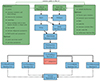 |
Fig. A.1. General flowchart of the OneCovariance code. The green boxes indicate files that are fed to the code (visit the readthedocs webpage, https://onecovariance.readthedocs.io/en/latest/index.html, for a more detailed discussion). The dashed lines with arrows indicate that files or functionalities are included, but not inherited. The solid arrows instead indicate inheritance. Each blue box indicates a python module in the form of a class with the corresponding name. The red box is a C++ class wrapped into python with pybind to carry out some of the heavy lifting in the code. Section numbers indicate where the corresponding equations and description of the content of each module can be found in the paper. |
Appendix B: Spherical harmonic decomposition
A two-dimensional field  can be expanded in a spherical harmonic basis:
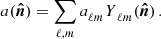 (B.1)
(B.1)
The spherical harmonics,  , satisfy the orthogonality relation
 (B.2)
(B.2)
with the solid angle element dΩn associated with  . Furthermore, we use the following Fourier space convention:
 (B.3)
(B.3)
With this definition, the Fourier components of statistically homogeneous fields have the following n-point statistics
 (B.4)
(B.4)
where k1…n≔k1+…+kn. Using the Rayleigh expansion, the exponential can be written as
 (B.5)
(B.5)
where x=|x| is the absolute value and  the angular part of the vector x, likewise for k.
Appendix C: Polyspectra on the sphere
Expanding the expression using Equation (B.1), Equation (B.4) and Equation (B.5) yields
 (C.1)
(C.1)
where we carried out the angular integrals  and used the orthonormality of the spherical harmonics. Angular integrations over spherical harmonics are trivially evaluated casting Equation (C.1) into a form respecting rotational symmetries. For Equation (8) this is for example realised by the diagonality in ℓ and m. To make further progress, we expand the delta distribution into plane waves as well:
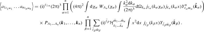 (C.2)
(C.2)
Here we defined the integral over spherical harmonics,
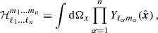 (C.3)
(C.3)
which can be decomposed into integrals over two and three spherical harmonics using
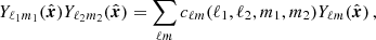 (C.4)
(C.4)
with the Klebsch-Gordon coefficients
 (C.5)
(C.5)
and the Gaunt integral  :
:
 (C.6)
(C.6)
The angular polyspectrum,  , is then defined via
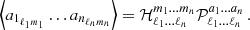 (C.7)
(C.7)
For n=2, 3 the functional form of the angular polyspectrum is completely fixed by rotational symmetry since the integral over Ωk can always be evaluated.
Appendix D: Flat sky approximation
For computational simplicity, one often relies not on a spherical harmonic decomposition but rather a flat two-dimensional discrete Fourier transform by replacing the directional vector  by a unit vector in the flat sky
  . In this flat sky, one can decompose the projected field a into Fourier modes
 (D.1)
(D.1)
where As is the area of the flat sky patch. The sum runs over all  , where
  . For As→∞ we can replace the discrete by a continuous Fourier transformation, such that
 (D.2)
(D.2)
The corresponding angular power spectra are defined via
 (D.3)
(D.3)
for the discrete and continuous cases respectively, where δD(x−y) is the Dirac δ-distribution. Higher-order correlators follow analogously.
Appendix E: Halo profiles
For an NFW profile (Navarro et al. 1997) the Fourier transform assumes the form
![Mathematical equation: $$ \tilde u(k|M,z) = \cos (kr_\mathrm {s})\left [\mathrm {Ci}(k(1+c)r_\mathrm {s}) - \mathrm {Ci}(kr_\mathrm {s})\right ] -\frac {\sin (ckr_\mathrm {s})}{kr_\mathrm {s}(1+c)} + \frac {\sin (kr_\mathrm {s})\left (\mathrm {Si}(kr_\mathrm {s}(1+c))-\mathrm {Si}(kr_\mathrm {s})\right )}{\frac {1}{1+c} +\ln (1+c) -1}\,, $$](/articles/aa/full_html/2025/07/aa52592-24/aa52592-24-eq184.gif) (E.1)
(E.1)
where Si(x) and Ci(x) are sine and cosine integrals. The scaling radius
 (E.2)
(E.2)
defines the empirical concentration relation c(M); here ΔV is the virial overdensity. It should be noted that Equation (15) can, in principle, include an integral over the concentration. However, assuming a mean relation between c and M, allows for analytic integration. For the baseline functional form, we assume the relation provided in Duffy et al. (2008):
![Mathematical equation: $$ c(M,z) = 10.14\left [\frac {M}{2\times 10^{12}h^{-1}M_\odot }\right ]^{-0.81} (1+z)^{-1.01}\,. $$](/articles/aa/full_html/2025/07/aa52592-24/aa52592-24-eq186.gif) (E.3)
(E.3)
Appendix F: Mixed term reconsidered
It should be noted that the equations in Sect 5.2 for the mixed term Equation (66) and the non-Gaussian term assume the tracers to be uniformly distributed. This will not be fulfilled when estimating the statistics in a realistic survey with a nontrivial angular mask and depth variations across the survey footprint. Schneider et al. (2002) have derived the corresponding equations for the shear correlation functions from which we reproduce the mixed term of  for a tomographic setup,
![Mathematical equation: $$ \mathrm {Cov}_{\mathrm {G,mix}} [{\hat {\xi }}_+^{(a_2a_2)}(\bar {\theta }_1);{\hat {\xi }}_+^{(a_3a_4)}(\bar {\theta }_2)] \equiv \; \frac {\sigma ^2_{\epsilon _1}}{N_\mathrm {pair}^{(a_1a_2)}(\bar {\theta }_1) \ \ N_\mathrm {pair}^{(a_3a_4)}(\bar {\theta }_2)} \ $$](/articles/aa/full_html/2025/07/aa52592-24/aa52592-24-eq188.gif) (F.1)
(F.1)
![Mathematical equation: $$ \times \; \Bigg [ \sum _{i,j,k}^{N_{a_1},N_{a_2},N_{a_3}} w^2_i w_j w_k \ \xi _+^{(a_2a_3)}(\theta _{jk}) \ \Delta _{\theta _1}(\theta _{ij})\Delta _{\theta _2}(\theta _{ik}) \ \delta ^{{\cal {{K}}}}_{a_1a_4} + \ 3 \ \mathrm {perm.}\Bigg ] \ , $$](/articles/aa/full_html/2025/07/aa52592-24/aa52592-24-eq189.gif) (F.2)
(F.2)
where the indices i,j,k stand for the individual galaxies having weights wi, the summation runs over all  galaxies residing in the aith tomographic redshift bin and
  denotes the angular bin selection function which is unity iff θij≡|θi−θj|∈θ.
For an efficient evaluation of the triplet sums we proceed along the lines of Slepian & Eisenstein (2015) and decompose the three-point correlator in its multipoles:
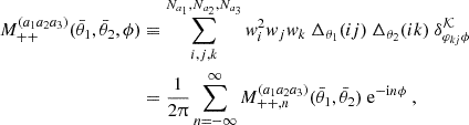 (F.3)
(F.3)
where φji denotes the polar angle of θij, ϕ≡φki−φji and the multipole components can be calculated as
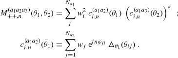 (F.4)
(F.4)
To further speed up the computation we make use of the combined estimator method introduced in Porth et al. (2024) that amends the equations presented here with grid-based methods for which the  can be computed via FFTs.
Once the multipoles are computed, we can perform the numerical integral to obtain
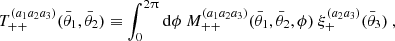 (F.5)
(F.5)
where we evaluate the shear correlation function at  . Plugging everything together we arrive at an approximation of Equation (F.1) in which ξ+ is not evaluated for every triplet, but instead the mean distance across the bin is taken18,
![Mathematical equation: $$ \mathrm {Cov}_{\mathrm {G,mix}} \left [{\hat {\xi }}_+^{(a_2a_2)}(\bar {\theta }_1);{\hat {\xi }}_+^{(a_3a_4)}(\bar {\theta }_2)\right ] \approx \frac {\sigma ^2_{\epsilon _1}}{N_\mathrm {pair}^{(a_1a_2)}(\bar {\theta }_1) \ \ N_\mathrm {pair}^{(a_3a_4)}(\bar {\theta }_2)} \ \ \left [T_{++}^{(a_1a_2a_3)}(\bar {\theta }_1, \bar {\theta }_2) \ \delta ^{{\cal {{K}}}}_{a_1a_4} + \ 3 \ \mathrm {perm.}\right ] \ . $$](/articles/aa/full_html/2025/07/aa52592-24/aa52592-24-eq197.gif) (F.6)
(F.6)
Performing similar computations we can also work out a multipole-based decomposition for the mixed covariance of  :
:
![Mathematical equation: $$ \mathrm {Cov}_{\mathrm {G,mix}} \left [{\hat {\xi }}_-^{(a_2a_2)}(\bar {\theta }_1);{\hat {\xi }}_-^{(a_3a_4)}(\bar {\theta }_2)\right ] \approx \frac {\sigma ^2_{\epsilon _1}}{N_\mathrm {pair}^{(a_1a_2)}(\bar {\theta }_1) \ \ N_\mathrm {pair}^{(a_3a_4)}(\bar {\theta }_2)} \ \ \left [T_{--}^{(a_1a_2a_3)}(\bar {\theta }_1, \bar {\theta }_2) \ \delta ^{{\cal {{K}}}}_{a_1a_4} + \ 3 \ \mathrm {perm.}\right ] \ , $$](/articles/aa/full_html/2025/07/aa52592-24/aa52592-24-eq199.gif) (F.7)
(F.7)
where the T−− are given as
![Mathematical equation: $$ \begin{aligned}T_{--}^{(a_1a_2a_3)}(\bar {\theta }_1, \bar {\theta }_2) &\equiv \int _0^{2\pi } \mathrm {d} \phi \ M_{--}^{(a_1a_2a_3)}(\bar {\theta }_1, \bar {\theta }_2,\phi ) \ \xi _+^{(a_2a_3)}(\bar {\theta }_3) \ ; \\ M_{--}^{(a_1a_2a_3)}(\bar {\theta }_1, \bar {\theta }_2,\phi ) &\equiv \frac {1}{2} \sum _{i=1}^{N_{a_1}}{{\mathit {w}}}_i^2\left\{ c_{i,4+n}^{(a_1,a_2)}(\bar {\theta }_1)\left [c_{i,4+n}^{(a_1,a_3)}(\bar {\theta }_2)\right ]^* + c_{i,n-4}^{(a_1,a_2)}(\bar {\theta }_1)\left [c_{i,n-4}^{(a_1,a_3)}(\bar {\theta }_2)\right ]^*\right\} \ . \end{aligned} $$](/articles/aa/full_html/2025/07/aa52592-24/aa52592-24-eq200.gif) (F.8)
(F.8)
Appendix G: Bandpowers
Band powers are angular averages over the angular power spectrum, Equation (8), and can as such make more use of the easier calculations in harmonic space, while including effects of survey mask and finite coverage of scales more accessible. Generally, they are defined as
 (G.1)
(G.1)
where SL is the band power response function and  is the normalisation
 (G.2)
(G.2)
such that the band powers trace the angular power  at the log-centered bins in L. Due to the orthogonality of the Bessel functions, Equation (56) and Equation (57) can be inverted to express the band powers in terms of the real space correlation functions w, γt and ξ±. Thus, by using Equation (G.1), one finds (Schneider et al. 2002)
 (G.3)
(G.3)
 (G.4)
(G.4)
![Mathematical equation: $$ {\cal {{C}}}_{\epsilon _i\epsilon _j{\mathrm {E/B}}}({L}) = \; \frac {\uppi }{{\cal {{N}}}_L}\; \int \theta \mathrm {d}\theta \; T(\theta ) \left [\xi _+^{(ij)}(\theta )\; g_+^L(\theta ) \pm \xi _-^{(ij)}(\theta )\; g_-^L(\theta ) \right ]\,, $$](/articles/aa/full_html/2025/07/aa52592-24/aa52592-24-eq207.gif) (G.5)
(G.5)
for GC, GGL, and CS respectively. Where the E-mode corresponds to the sum and the B-mode to the difference. With ‘+’ corresponding to J0, the kernels are given by
 (G.6)
(G.6)
 (G.7)
(G.7)
If the real-space correlation functions are only accessible over a finite range of angular separations, one apodises the kernels with a Hann window (see Joachimi et al. 2021):
![Mathematical equation: $$ T(\theta ) = \begin {cases}\;\cos ^2 \left (\frac {\uppi [x- (x_{\mathrm {lo}}+\Delta _x/2)]}{2\Delta _x} \right ) &\quad {\textrm {if}} \quad x_{\mathrm {lo}} -\frac {\Delta _x}{2} \leq x < x_{\mathrm {lo}} +\frac {\Delta _x}{2} \\ \;1 &\quad {\textrm {if}}\quad x_{\mathrm {lo}} +\frac {\Delta _x}{2} \leq x < x_{\mathrm {up}} -\frac {\Delta _x}{2} \\ \;\cos ^2 \left (\frac {\uppi [x-(x_{\mathrm {up}} - \Delta _x/2)]}{2\Delta _x} \right ) &\quad {\textrm {if}} \quad x_{\mathrm {up}} -\frac {\Delta _x}{2} \leq x < x_{\mathrm {up}} +\frac {\Delta _x}{2}\\ \; 0 &\quad \quad \quad \quad \quad \quad {\textrm {else}} \end {cases} \,, $$](/articles/aa/full_html/2025/07/aa52592-24/aa52592-24-eq210.gif) (G.8)
(G.8)
with x=logθ and Δx the logarithmic bandwidth. The apodisation is such that the lower and upper limit is centred on xlo=logθlo and xup=logθup, respectively.
Here we chose the band power response to be a top hat between ℓlo,l and ℓup,l leading to a normalisation  and a closed form for
  and hL:
![Mathematical equation: $$ g_+^L(\theta ) = \frac {1}{\theta ^2} \left [\theta \ell _{{\mathrm {up}},L}\; {\mathrm {J}}_1(\theta \ell _{{\mathrm {up}},L}) - \theta \ell _{{\mathrm {lo}},L}\; {\mathrm {J}}_1(\theta \ell _{{\mathrm {lo}},L})\right ] \,, $$](/articles/aa/full_html/2025/07/aa52592-24/aa52592-24-eq213.gif) (G.9)
(G.9)
![Mathematical equation: $$ g_-^L(\theta ) = \frac {1}{\theta ^2} \left [{\cal {{G}}}_-(\theta \ell _{{\mathrm {up}},L}) - {\cal {{G}}}_-(\theta \ell _{{\mathrm {lo}},L}) \right ]\,, $$](/articles/aa/full_html/2025/07/aa52592-24/aa52592-24-eq214.gif) (G.10)
(G.10)
![Mathematical equation: $$ h^L = -\frac {1}{\theta ^2}\left [\theta \ell _{{\mathrm {up}},L} \mathrm {J}_1(\theta \ell _{{\mathrm {up}},L}) - \theta \ell _{{\mathrm {lo}},L}\mathrm {J}_1(\theta \ell _{{\mathrm {lo}},L}) + 2\mathrm {J}_0(\theta \ell _{{\mathrm {up}},L}) - 2\mathrm {J}_0(\theta \ell _{{\mathrm {lo}},L})\right ]\,, $$](/articles/aa/full_html/2025/07/aa52592-24/aa52592-24-eq215.gif) (G.11)
(G.11)
where
 (G.12)
Linking the band powers directly to the angular power spectra yields the final expressions
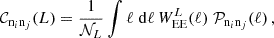 (G.13)
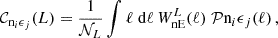 (G.14)
![Mathematical equation: $$ {\cal {{C}}}_{\epsilon _i\epsilon _j{\mathrm {E}}}(L) = \frac {1}{{2\cal N}_L} \int \ell \;\mathrm {d} \ell \, \left [W^L_{\mathrm {EE}}(\ell )\; {\cal {{P}}}_{\epsilon _i\epsilon _j,\mathrm {E}}(\ell ) + W^L_{\mathrm {EB}}(\ell )\; {\cal {{P}}}_{\epsilon _i\epsilon _j,\mathrm {B}}(\ell ) \right ] \,, $$](/articles/aa/full_html/2025/07/aa52592-24/aa52592-24-eq219.gif) (G.15)
(G.15)
![Mathematical equation: $$ {\cal {{C}}}_{\epsilon _i\epsilon _j{\mathrm {B}}} (L) = \frac {1}{2 {\cal {{N}}}_L} \int \ell \;\mathrm {d} \ell \, \left [W^L_{\mathrm {BE}}(\ell )\; {\cal {{P}}}_{\epsilon _i\epsilon _j,\mathrm {E}}(\ell ) + W^L_{\mathrm {BB}}(\ell )\; {\cal {{P}}}_{\epsilon _i\epsilon _j,\mathrm {B}}(\ell ) \right ]\,, $$](/articles/aa/full_html/2025/07/aa52592-24/aa52592-24-eq220.gif) (G.16)
(G.16)
with kernels given by
![Mathematical equation: $$ W^L_{\mathrm {EE}}(\ell ) = W^L_{\mathrm {BB}}(\ell ) = \!\! \int \!\! \theta \;\mathrm {d} \theta \, T(\theta ) \left [{\mathrm {J}}_0(\ell \theta )\; g_+^L(\theta ) + {\mathrm {J}}_4(\ell \theta )\; g_-^L(\theta ) \right ]\,, $$](/articles/aa/full_html/2025/07/aa52592-24/aa52592-24-eq221.gif) (G.17)
(G.17)
![Mathematical equation: $$ W^L_{\mathrm {EB}}(\ell ) = W^L_{\mathrm {BE}}(\ell ) = \!\! \int \!\! \theta \;\mathrm {d} \theta \, T(\theta ) \left [{\mathrm {J}}_0(\ell \theta )\; g_+^L(\theta ) - {\mathrm {J}}_4(\ell \theta )\; g_-^L(\theta ) \right ] \,, $$](/articles/aa/full_html/2025/07/aa52592-24/aa52592-24-eq222.gif) (G.18)
(G.18)
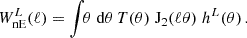 (G.19)
Appendix H: COSEBIs and Ψ statistics
The complete orthogonal sets of E/B-integrals (COSEBIs, Schneider et al. 2010) are summary statistics for CS, avoiding leakage between E- and B-modes on a finite range of angular scales. These are discrete values and can be directly linked to the two-point correlation functions:
![Mathematical equation: $$ E^{(ij)}_n = \frac {1}{2} \int _{\theta _{\mathrm {min}}}^{\theta _{\mathrm {max}}} \theta \;\mathrm {d}\theta \; [T_{+n}(\theta )\,\xi ^{(ij)}_+(\theta ) + T_{-n}(\theta )\,\xi ^{(ij)}_-(\theta )]\,, $$](/articles/aa/full_html/2025/07/aa52592-24/aa52592-24-eq224.gif) (H.1)
(H.1)
![Mathematical equation: $$ B^{(ij)}_n = \frac {1}{2} \int _{\theta _{\mathrm {min}}}^{\theta _{\mathrm {max}}}\theta \;\mathrm {d}\theta \; [T_{+n}(\theta )\,\xi ^{(ij)}_+(\theta ) - T_{-n}(\theta )\,\xi ^{(ij)}_-(\theta )]\,. $$](/articles/aa/full_html/2025/07/aa52592-24/aa52592-24-eq225.gif) (H.2)
(H.2)
The filter functions T±n(θ) are defined for a given angular range, θ∈[θmin, θmax]. Two families of COSEBIs have been used in the past, linear-COSEBIs and log-COSEBIs, defining whether the oscillations of T±(θ) are linearly or logarithmically spaced respectively. The COSEBIs are labelled by n natural numbers, with filters having n+1 roots in their range of support. Here, we employ log-COSEBIs, but the code can use any filter function. The theoretical model prediction for COSEBIs is given by
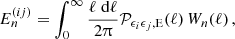 (H.3)
(H.3)
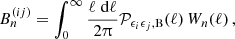 (H.4)
(H.4)
where the weight functions, Wn(ℓ), are Hankel transforms of T±(θ)
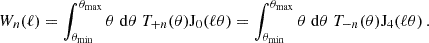 (H.5)
(H.5)
A very similar set of observables can be constructed for GGL and GC (Buddendiek et al. 2016; Asgari et al. 2021a) to avoid including physical scales outside [θmin,θmax]. Similarly to the COSEBIs, they are defined as
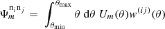 (H.6)
(H.6)
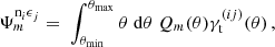 (H.7)
(H.7)
so that Um(θ) is compensated and orthogonal and Qm(θ) given by the expression
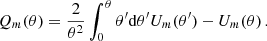 (H.8)
(H.8)
Their respective Fourier counterparts are calculated in the same manner as the COSEBIs E-mode, Equation (H.3), with a Fourier weight:
 (H.9)
(H.9)
Appendix I: Definition of Fourier and real space filters for summary statistics
As an example, we define the linear maps WL(ℓ) and RL(θ) for the three summary statistics considered in Section 5. For real space correlation functions, one finds the following:
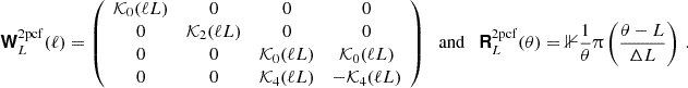 (I.1)
(I.1)
Here π is a top-hat filter centred around L with bandwidth ΔL. This includes the averaging over θ bins in the weights. For bandpowers one finds
 (I.2)
(I.2)
and for COSEBIs:
 (I.3)
(I.3)
We now label components of vec(C)(ℓ) with Latin indices and similar for WL(ℓ) and the summary statistic  . Using Equation (51) and Equation (45), Gaussian covariances which are not pure shot noise terms can be expressed as
![Mathematical equation: $$ \mathrm {Cov}_\mathrm {G, sva}\left [{\cal {{O}}}^{ij}_{p_1,L_1}{\cal {{O}}}^{mn}_{p_2,L_2}\right ] = \;\frac {1}{2 \uppi \; \mathrm {max}(A_{(ij)}A_{(mn)}) } \sum _{q_1,q_2} \int \ell \mathrm {d}\ell \left (\boldsymbol {{\mathbf {{\mathsf{W}}}}}_{L_1}(\ell )\right )_{p_1q_1}\left (\boldsymbol { {\mathbf {{\mathsf{W}}}}}_{L_2}(\ell ) \right )_{p_2q_2} $$](/articles/aa/full_html/2025/07/aa52592-24/aa52592-24-eq237.gif) (I.4)
(I.4)
![Mathematical equation: $$ \times \left [{\cal {{P}}}^{(im)}(\ell ) {\cal {{P}}}^{(jn)}(\ell ) + {\cal {{P}}}^{(in)}(\ell ) {\cal {{P}}}^{(jm)}(\ell ) \right ]_{q_1q_2} $$](/articles/aa/full_html/2025/07/aa52592-24/aa52592-24-eq238.gif) (I.5)
(I.5)
where it is understood that the summary statistic i is the one identified with the tracer combination a1,a2 and the same of j and a3,a4. The shot noise term can then be calculated as
![Mathematical equation: $$ \mathrm {Cov}_\mathrm {G, sn}\left [{\cal {{O}}}^{ij}_{p_1,L_1}{\cal {{O}}}^{mn}_{p_2,L_2}\right ] = \sum _q N^{ij}_q\int \frac {\theta ^2\mathrm {d}\theta }{n^{ij}_q(\theta )} \left (\boldsymbol {{\mathbf {{\mathsf{R}}}}}_{L_1}(\theta )\right )_{p_1q}\left (\boldsymbol {{\mathbf {{\mathsf{R}}}}}_{L_2}(\theta )\right )_{p_2q} \left [\delta ^\mathrm {K}_{im}\delta ^\mathrm {K}_{jn} + \delta ^\mathrm {K}_{in}\delta ^\mathrm {K}_{jm}\right ]\,, $$](/articles/aa/full_html/2025/07/aa52592-24/aa52592-24-eq239.gif) (I.6)
(I.6)
where  is the differential pair-count density and
  the noise level in the q-th summary statistic and the i,j tomographic bin combination. Lastly, connected terms such as NG and SSC are given by
![Mathematical equation: $$ \mathrm {Cov}_\mathrm {NG, sn}\left [{\cal {{O}}}^{ij}_{p_1,L_1}{\cal {{O}}}^{mn}_{p_2,L_2}\right ] = \; \frac {1}{4 \uppi ^2 \mathrm {max}(A_{(ij)}A_{(mn)}) } \sum _{q_1,q_2} \int \mathrm {d} \ell _1\, \ell _1\; \int \mathrm {d} \ell _2\, \ell _2\; \left (\boldsymbol {{\mathbf {{\mathsf{W}}}}}_{L_1}(\ell _1)\right )_{p_1 q_1 }\left (\boldsymbol {{\mathbf {{\mathsf{W}}}}}_{L_2}(\ell _2)\right )_{p_2 q_2} $$](/articles/aa/full_html/2025/07/aa52592-24/aa52592-24-eq242.gif) (I.7)
(I.7)
![Mathematical equation: $$ \begin{aligned}&\times \int _0^\uppi \frac {\mathrm {d} \phi _\ell }{\uppi } \; T^{(ij)(mn)}_{q_1 q_2}(\boldsymbol {\ell }_1,-\boldsymbol {\ell }_1,\boldsymbol {\ell }_2,-\boldsymbol {\ell }_2)\,, \\ \mathrm {Cov}_\mathrm {SSC, sn}\left [{\cal {{O}}}^{ij}_{p_1,L_1}{\cal {{O}}}^{mn}_{p_2,L_2}\right ] = &\;\frac {1}{4 \uppi ^2} \int \mathrm {d} \ell _1\, \ell _1\; \int \mathrm {d} \ell _2\, \ell _2\; \left (\boldsymbol {{\mathbf {{\mathsf{W}}}}}_{L_1}(\ell _1)\right )_{p_1 q_1 }\left (\boldsymbol {{\mathbf {{\mathsf{W}}}}}_{L_2}(\ell _2)\right )_{p_2 q_2} \left (T^{(ij)(mn)}_\mathrm {SSC}({\ell _1,\ell _2})\right )_{q_1 q_2}\,. \end{aligned} $$](/articles/aa/full_html/2025/07/aa52592-24/aa52592-24-eq243.gif) (I.8)
(I.8)
All Tables
Fiducial choice of cosmological parameters within ΛCDM used for the forward simulations to test the signal and noise modelling for KiDS-Legacy-like. The given cosmology is equivalent to S8≡σ8[(Ωb+Ωc)/0.3]1/2=0.82. The parameters are set in accordance with the constraints from KiDS-1000 (Asgari et al. 2021b), while σ8 is set to be the mid-value between KiDS-1000 and Planck (Planck Collaboration VI 2020).
All Figures
|
Fig. 1. Effect of different choices for the covariance modelling for the inference of S8 using the KiDS-Legacy data. Shown is the marginal maximum posterior and the corresponding 68% intervals (one σ) interval normalised to the fiducial settings assuming realistic pair counts and including feedback parametrised by TAGN via hmcode2020 (Mead et al. 2020), the SSC and nG contributions, an idealised mixed term, a realistic survey mask, and the NLA model. Each blue data point replaces one of those assumptions at a time. Left: real space correlation functions. Right: bandpowers. |
| In the text | |
|
Fig. 2. KiDS-Legacy-like covariance matrix for COSEBIs. The diagonals are in the following order i≤j with the tomographic bin indices i and j and in each little sub-block the order of the COSEBIs runs over n=1,…,5. Furthermore, we omit the B-mode signal here, since it is pure shape noise in the case of COSEBIs. The six different panels show the relative contribution of each term to the total covariance. In particular, we show the super-sample covariance (SSC), the non-Gaussian (nG), and the Gaussian (G) contribution in the upper three panels (compare Equations (2), and (3)). The lower three panels show the three components of the Gaussian contribution, the sample variance (sva), the mixed term (mix), and the shape or shot noise term (sn), as described in Equation (6). |
| In the text | |
|
Fig. 3. Cosmic shear setup with the six KiDS-Legacy tomographic bins. The colour bar shows the tomographic bin index combination, I (i.e. for tomographic bins i, j the index is |
| In the text | |
|
Fig. 4. Relative difference between the signal measured in the 4224 Egretta mocks (realistic mask and depth variations) with the signal prediction of OneCovariance code. The colour bar indicates the different unique tomographic bin combinations, the same as in Figure 3. The dashed lines show ξ− and solid lines ξ+. The grey band indicates a five per cent relative difference. The different plots show varying settings in the OneCovariance code. In particular, we distinguish whether the averaging over the θ bin (see Equation (61)) is carried out and if the pixel window due to the finite resolution of the healpix map is taken into account, i.e. damping power on small scales (Nside correction). |
| In the text | |
|
Fig. 5. KiDS-Legacy covariance matrix for real space correlation functions. Each square represents a unique combination of tomographic bins and contains the covariance for that combination in nine angular bins between 0.5 and 300 arcmin. The diagonals are in the order i≤j with the tomographic bin indices i and j. Left: correlation coefficient of the full covariance matrix without multiplicative shear bias uncertainty. In the lower triangle, the analytic covariance is shown, while the upper triangle shows the covariance as measured in the Egretta mocks (realistic mask and depth variations). Right: relative impact of the new mixed term (see Appendix F) on the Gaussian part covariance matrix compared to an idealised mixed term with a homogeneous pair and triplet counts. The latter were directly estimated from the KiDS-Legacy-like catalogue. |
| In the text | |
|
Fig. 6. Relative difference between the standard deviation of the Egretta mocks (realistic mask and depth variations) and that from the analytic covariance matrix from the OneCovariance code for the same setting as Figure 5. The dashed lines show ξ− and solid lines depict ξ+. The tomographic bin combination is shown in the top left corner of each subplot. |
| In the text | |
|
Fig. 7. Showcase of the consistency tests possible with the OneCovariance code. This is a cosmic shear setting as in KiDS-1000 (Asgari et al. 2021b) (i.e. five tomographic bins, eight band power bins, five modes for COSEBIs, and nine bins for ξ±. The code was used to create the full covariance matrix for any pair of those three statistics. Since these are all summary statistics for the same tracer and almost over the same physical scales, the matrix is close to being singular. The full matrix shown here has a single negative eigenvalue originating from numerical noise. However, the subcovariance matrices between each pair of summary statistics are still positive-definite. We do not show the B modes for COSEBIs and bandpowers since they mainly consist of shape noise (although they are still highly correlated with the shape noise of the other statistics). |
| In the text | |
|
Fig. 8. Left: redshift distribution of the target sample for five tomographic bins of KiDS-1000 as solid lines. The grey bars indicate the reference sample. Right: Pearson correlation coefficient with the lower triangle showing the predictions of the analytical prescription, Equation (91), while the upper triangle shows the results obtained by jackknife resampling from Hildebrandt et al. (2021) (compare their Figure 3). |
| In the text | |
|
Fig. 9. Left: auto-correlation angular power spectra of the reference sample as a function of spectroscopic redshift (colour bar). The solid lines use the Limber approximation, Equation (10), while the dashed lines make use of the full expression, Equation (8). Right: fractional difference as a percentage of the Gaussian covariance term when using Limber vs non-Limber. |
| In the text | |
|
Fig. 10. Left: contribution to the standard deviation of the clustering redshift measurements. The solid lines correspond to the total variance, the dashed lines to the non-Gaussian contribution, and the dotted lines to the shot noise. For all tests, we ignored the SSC term since it is suppressed for galaxy clustering. Right: comparison of the analytical standard deviation (solid lines) with the simulations (symbols). |
| In the text | |
|
Fig. A.1. General flowchart of the OneCovariance code. The green boxes indicate files that are fed to the code (visit the readthedocs webpage, https://onecovariance.readthedocs.io/en/latest/index.html, for a more detailed discussion). The dashed lines with arrows indicate that files or functionalities are included, but not inherited. The solid arrows instead indicate inheritance. Each blue box indicates a python module in the form of a class with the corresponding name. The red box is a C++ class wrapped into python with pybind to carry out some of the heavy lifting in the code. Section numbers indicate where the corresponding equations and description of the content of each module can be found in the paper. |
| In the text | |
Current usage metrics show cumulative count of Article Views (full-text article views including HTML views, PDF and ePub downloads, according to the available data) and Abstracts Views on Vision4Press platform.
Data correspond to usage on the plateform after 2015. The current usage metrics is available 48-96 hours after online publication and is updated daily on week days.
Initial download of the metrics may take a while.