| Issue |
A&A
Volume 698, June 2025
|
|
|---|---|---|
| Article Number | A217 | |
| Number of page(s) | 21 | |
| Section | Cosmology (including clusters of galaxies) | |
| DOI | https://doi.org/10.1051/0004-6361/202554017 | |
| Published online | 17 June 2025 | |
KiDS-1000: Detection of deviations from a purely cold dark matter power spectrum with tomographic weak gravitational lensing
1
Universität Bonn, Argelander-Institut für Astronomie, Auf dem Hügel 71, 53121 Bonn, Germany
2
Waterloo Centre for Astrophysics, University of Waterloo, Waterloo, ON N2L 3G1, Canada
3
Department of Physics and Astronomy, University of Waterloo, Waterloo ON N2L 3G1, Canada
4
Leiden Observatory, Leiden University, Einsteinweg 55, 2333 CC Leiden, The Netherlands
⋆ Corresponding author: This email address is being protected from spambots. You need JavaScript enabled to view it.
Received:
4
February
2025
Accepted:
14
April
2025
Abstract
Model uncertainties in the non-linear structure growth limit current probes of cosmological parameters. To shed more light on the physics of non-linear scales, we reconstructed the finely binned three-dimensional power-spectrum from lensing data of the Kilo-Degree Survey (KiDS), relying solely on the background cosmology, the source redshift distributions, and the intrinsic alignment (IA) amplitude of sources (and their uncertainties). The adopted Tikhonov regularisation stabilises the deprojection, enabling a Bayesian reconstruction in separate z-bins. Following a detailed description of the algorithm and performance tests with mock data, we present our results for the power spectrum as relative deviations from a ΛCDM reference spectrum that includes only structure growth by cold dark matter. Averaged over the full range z ≲ 1, a Planck-consistent reference then requires a significant suppression on non-linear scales, k = 0.05–10 h Mpc−1, of up to 20%–30% to match KiDS-1000 (68% credible interval, CI). Conversely, a reference with a lower S8 ≈ 0.73 avoids suppression and matches the KiDS-1000 spectrum within a 20% tolerance. When resolved into three z-bins, however, and regardless of the reference, we detect structure growth only in the range z ≈ 0.4–0.13, but not in the range z ≈ 0.7–0.4. This could indicate spurious systematic errors in KiDS-1000, inaccuracies in the intrinsic alignment (IA) model, or potentially a non-standard cosmological model with delayed structure growth. In the near future, analysing data from Stage IV surveys with our algorithm promises a substantially more precise reconstruction of the power spectrum.
Key words: gravitational lensing: weak / cosmology: observations / dark matter / large-scale structure of Universe
© The Authors 2025
 Open Access article, published by EDP Sciences, under the terms of the Creative Commons Attribution License (https://creativecommons.org/licenses/by/4.0), which permits unrestricted use, distribution, and reproduction in any medium, provided the original work is properly cited.
This article is published in open access under the Subscribe to Open model. This email address is being protected from spambots. You need JavaScript enabled to view it. to support open access publication.
1. Introduction
In contrast to the continuous background expansion of the Universe, the structure growth in the matter density field is less certain, with uncertainties in theoretical models that vary by 10% or more in the non-linear regime through their dependence on baryon-galaxy feedback; possible deviations from purely cold, stable, and interaction-free dark matter; or, perhaps, modifications in the standard model of gravity (e.g., Laguë et al. 2024; Bucko et al. 2024; Mauland et al. 2024; Ferreira et al. 2024; Salcido et al. 2023; Schneider et al. 2022; Harnois-Déraps et al. 2015; Smith & Markovic 2011; Jing et al. 2006, and references therein). Currently the theory uncertainties are limiting studies of cosmological parameters because they often rely on measures of the cosmic structure, such as the matter power spectrum, Pδ(k, z), at different redshifts, z = :1/a − 1, and spatial (comoving) wave number, k (e.g., Pranjal et al. 2025; García-García et al. 2024; Secco et al. 2022; Li et al. 2023; Asgari et al. 2021; Heymans et al. 2013). To shed more light on the physics imprinted on non-linear scales, direct measurements of a model-free Pδ(k, z) with a minimum of assumptions promise to be a valuable model test. That this is already feasible for z ≲ 1 and 10−2 ≲ k/(h Mpc−1)≲10 with Stage III galaxy surveys when exploiting the weak gravitational lensing effect, such as with KiDS-1000 (Kuijken et al. 2019, 2015), is shown in this work. This foreshadows exciting applications to future lensing data, such as those by Euclid (Euclid Collaboration: Mellier et al. 2025), the Vera C. Rubin Observatory Legacy Survey of Space and Time (The LSST Dark Energy Science Collaboration 2018), or the Nancy Grace Roman Space Telescope (Spergel et al. 2015).
The coherent distortion of distant galaxy images, just sources hereafter, by the weak shearing of light bundles passing through intervening foreground structure probes the matter power spectrum (for a review, see, e.g., Kilbinger 2015; Schneider 2006; Bartelmann & Schneider 2001). More specifically, and putting negligible higher-order corrections aside (Hilbert et al. 2009), the second-order correlations, ξ±(θ), at lag θ in the cosmic shear field are simply a linear projection of Pδ(k, z) throughout the look-back light cone up to the distance of the sources (Preston et al. 2024; Mezzetti et al. 2012; Simon 2012; Bacon et al. 2005; Pen et al. 2003; Tegmark & Zaldarriaga 2002; Seljak 1998). Therefore, by using ξ±(ij)(θ) between tomographic bins, i and j, for different characteristic distances of sources, the correlation data can be deprojected to recover, within limitations, the original Pδ(k, z). More conveniently, as in Simon (2012, S12), we focus on a transfer function, fδ(k, z) = Pδ(k, z)/Pδfid(k, z), with respect to a reference model, Pδfid(k, z), to highlight deviations from the presumed reference inside an average z-bin. For this reference, we chose a purely cold dark matter (CDM) model to probe for deviations, fδ(k, z)≠1, that may hint at missing physics in a basic, well-understood dark matter scenario or at unidentified systematic errors in the data. However, at the end of the day, the kind of reference is a deliberate choice.
Required for the deprojection, on the other hand, is the knowledge of the projection (lensing) kernel and the inclusion of the intrinsic alignment (IA) of sources in the correlation function, an essential part of modern cosmic-shear analyses (Hirata & Seljak 2004; Crittenden et al. 2001; Croft & Metzler 2000). The lensing kernel is fully described by the radial distribution of sources inside the tomographic bins; the average matter density in today’s Universe, Ωm, relative to the critical density, ρcrit = 3H02(8πGN)−1; and the expansion rate 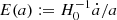 , where H0 = 100 h km s−1 Mpc−1 is the Hubble constant and GN is Newton’s gravitational constant. The kernel parameters Ωm and E(a) are confined to percentage precision by cosmological experiments already (E2(a)≈Ωm[a−3 − 1]+1 for a flat universe), especially owing to CMB experiments (Planck Collaboration VI 2020; Hinshaw et al. 2013), but also by combining probes from the closer Universe (e.g., Heymans et al. 2021; Abbott et al. 2018). Nevertheless, in the refinement of the method in S12 for KiDS-1000, we marginalised here over the small background cosmology uncertainties, and over those in the source distributions (Hildebrandt et al. 2021). Another refinement is the required inclusion of the IA, and its uncertainty, in the deprojection procedure by the widely employed non-linear alignment (NLA) model (Joachimi et al. 2011; Bridle & King 2007), informed by the IA constraints in Asgari et al. (2021).
Despite the simplicity of the well-defined projection, the noise level in ξ±(ij)(θ) makes the recovery of the matter power spectrum still challenging because the deprojection has to undo a convolution in radial and transverse direction, producing strongly correlated, oscillating noise in an unstable reconstruction. This complication could be mitigated by data volumes substantially larger than KiDS-1000, beating down oscillating noise, or by additional assumptions on the redshift dependence or shape of the power spectrum in fitting an analytical model with few parameters to the data (Perez Sarmiento et al. 2025; Ye et al. 2024; Truttero et al. 2025; Broxterman & Kuijken 2024; Preston et al. 2024, 2023; Pen et al. 2003; Seljak 1998). Avoiding analytical models, we instead propose constraining fδ(k, z) averages in different k- and z-bins, as in S12 but additionally filtered by a classic Tikhonov regularisation, for instance as applied in the mathematically related problem of deconvolving noisy images (e.g., Murata & Takeuchi 2022). In contrast to S12, the Tikhonov regularisation, installed on our Bayesian statistical model as prior, penalises strongly oscillating power spectra for noisy data, giving an advantage to solutions of fδ(k, z) that, on the one hand, are smoother in the k-direction, but, on the other hand, use no prior information on their z-dependence. We show with verification data that this regularisation indeed stabilises the reconstruction and extracts from KiDS-1000 data useful constraints on the transfer function fδ(k, z), either averaged over the full redshift range or averaged within three separate redshift bins to broadly probe a redshift evolution. Furthermore, for an efficient sampling of the posterior constraints of the matter power spectrum, we describe and test a Markov chain Monte Carlo (MCMC) code tailored to deal with the numerous 60 (or more) degrees-of-freedom of the binned, band power Pδ(k, z); its practical details are given in Appendix A.
The outline of the paper is as follows. Section 2 reviews our weak lensing formalism and shows that the projection of Pδ(k, z) into ξ±(ij)(θ), both binned, can be reduced to one projection matrix, to be reused as long as the same lensing kernel and IA parameters, including source redshift distributions, are employed. Section 3 defines the statistical model for our Bayesian analysis, including a prior for the Tikhonov regularisation. We summarise the KiDS-1000 data for our cosmic shear analysis in Sect. 4 and report our results in Sect. 5. Section 5 also reports, as verification of our reconstruction method, the results of a mock analysis based on KiDS-1000-like data produced by ray-tracing N-body data. Another verification test, this time based on the data vector of an analytical model subject to random noise, is presented in Appendix A. We discuss our results and conclusions on the reconstructed matter power spectrum in Sect. 6. Notably, our figures use comoving wave numbers, k, for spatial scales of the matter power spectrum, emphasised by the ‘c’ in the unit [k]=h cMpc−1.
2. Weak lensing formalism
This work is an application of the well-established theory of cosmic shear. For a review and its mathematical foundation, we refer to Kilbinger (2015) or Schneider (2006), and only briefly summarise our formalism here.
2.1. Cosmic shear
Weak gravitational lensing by fluctuations in the large-scale structure of the foreground matter density, 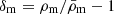 , distorts images of background galaxies. Their average shear distortion in direction θ of the sky shall be expressed by the complex γ(θ) = γ1(θ)+iγ2(θ) for an ensemble of galaxies with probability distribution function (PDF) pχ(χ) in comoving distance, χ. To lowest order, and sufficiently accurate in practical applications, the Fourier transform
  is related to the linear projection of fluctuations along θ,
![Mathematical equation: $$ \begin{aligned} \kappa (\boldsymbol{\theta }) = \frac{3H_0^2\,\Omega _{\rm m}}{2c^2}\, \int _0^{\chi _{\rm h}}\frac{\mathrm{d}\chi }{a(\chi )}\, \overline{W}(\chi )\,f_{\rm K}(\chi )\, \delta _{\rm m}\!\left[f_{\rm K}(\chi )\boldsymbol{\theta },\chi \right]\;, \end{aligned} $$](/articles/aa/full_html/2025/06/aa54017-25/aa54017-25-eq4.gif) (1)
(1)
through the convolution (ℓ ≠ 0)
 (2)
(2)
where c is the vacuum speed of light. In the above equations,  is the Fourier transform of the convergence κ(θ), the scalar fK(χ) is the (comoving) angular diameter distance for the curvature scalar K, the vector fK(χ)θ denotes a separation in a tangential plane on the sky at distance χ, the term 1 + z = a−1(χ) is our relation between redshift, z, and scale factor, a(χ), at the look back time of χ, and
 (3)
(3)
is the lensing efficiency, cut off at the size of the observable Universe, χh. As approximation, we assumed a flat sky with Cartesian coordinates for θ but expect negligible inaccuracies for angular separations below several degrees.
Practical estimators of γ(θ) in the direction θ of a galaxy image use a convenient definition of galaxy ellipticity, ϵ, that is calibrated to be an unbiased estimator, ⟨ϵ⟩=γ, for a selected source population (e.g., Giblin et al. 2021).
2.2. Second-order statistics
Our analysis exploits the coherent shear distortion of galaxy images over the sky to infer the three-dimensional power spectrum, Pδ(k, z), of matter density fluctuations inside the light cone,
 (4)
(4)
for a range of wave numbers and redshifts. The δD(x) denotes the Dirac delta function, and  is the Fourier coefficient of a fluctuation mode at redshift z inside the light cone. To obtain the power spectrum from γ(θ), we estimate the two-point correlation function of cosmic shear,
 (5)
(5)
at lag θ = |θ2 − θ1| from an ensemble of sources. Here, γt and γ× denote the tangential and cross-shear components relative to the orientation of θ2 − θ1 = :θ eiϕ on the sky, defined by γt + iγ× := −e−2iϕγ. In addition, using the hybrid extended Limber approximation in Fourier space (Kilbinger et al. 2017; Kaiser 1992), the correlation function of cosmic shear is a linear projection of Pδ(k, z),
 (6)
(6)
through the lensing kernel  – the minimal ingredient that has to be known to invert the projection. The expressions Jn(x) denote nth-order Bessel functions of the first kind, of which J0(x) has to be applied for ξ+ and J4(x) for ξ−.
2.3. Tomographic lensing and intrinsic alignment of sources
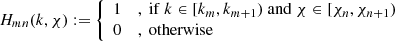
Owing to the information loss in the projection Eq. (6) for a single sample of sources, a power spectrum averaged over the entire light cone could be obtained at best, as in Pen et al. (2003) or Schneider et al. (2002). More advanced is splitting the source samples by redshift in a tomographic analysis for a better statistical precision, reflected by improved cosmology constraints in tomographic analyses, or to achieve a (limited) redshift resolution for the recovered Pδ(k, z). Therefore, we split our source sample into five redshift bins, using non-overlapping ranges of photometric redshifts, namely the zB-intervals (0.1, 0.3], (0.3, 0.5], (0.5, 0.7], (0.7, 0.9], and (0.9, 1.2], as done already in Hildebrandt et al. (2021). Figure 1 plots estimates of the resulting distributions pz(i)(z) for each bin i. The tomographic analysis then correlates the shear signal between bins i and j, denoted by the superscript “(ij)” in ξ±(ij)(θ). Compared to Eq. (6), this increases the data vector size by a factor of 5(5 + 1)/2 = 15 but also adds information on the Pδ(k, z) evolution because the shear tomography probes the same foreground with sources at different z.
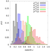 |
Fig. 1. Probability density distribution functions, pz(i)(z), of KiDS-1000 source galaxies within the five tomographic redshift bins (from i = 1 to i = 5): (0.1, 0.3], (0.3, 0.5], (0.5, 0.7], (0.7, 0.9], and (0.9, 1.2]. These estimates are from Hildebrandt et al. (2021). |
This tomographic analysis requires special attention with regard to additional contributions to the shear signal from the intrinsic alignment (IA) of sources (e.g., Lamman et al. 2024). In the ideal absence of IA, the orientations of intrinsic source ellipticities are statistically independent among each other and to the cosmic shear signal. So-called ‘II’ contributions, however, originate from correlated orientations of physically close galaxies. In addition, galaxy shapes are aligned to the surrounding matter density, giving rise to a ‘GI’ signal (Hirata & Seljak 2004). While II contributions could in principle be reduced by correlating only bin combinations with little radial overlap, and the GI signal could be suppressed by a nulling technique (Joachimi & Schneider 2008), we followed the common approach of modelling the II and GI signal in ξ±(ij)(θ) to avoid information loss,
 (7)
(7)
In this equation,
 (8)
(8)
is the ideal shear signal without IA. Covering both auto- (i = j) and cross-correlations (i ≠ j) of source samples, this expression is more general than Eq. (6). Herein, the lensing efficiency with superscript,  , refers to Eq. (3) but for the PDF pχ(i)(χ) of the ith bin. Notably, the pχ(i)(χ) are related to the pz(i)(z) in Fig. 1 by pχ(i)(χ) = pz(i)[z(χ)] |dz/dχ| for dz/dχ = H0 c−1 E[(1 + z)−1].
For the II and GI terms, we employed the NLA model by Joachimi et al. (2011), derived from the linear alignment model by Bridle & King (2007) but replacing the linear matter power-spectrum by the non-linear one. Clearly just tweaking the original linear IA model, the NLA is nevertheless sufficiently accurate to model contemporary lensing data (Harnois-Déraps et al. 2022), predicting
 (9)
(9)
for II correlations and for the GI term
 (10)
(10)
The amplitude of the IA signal scales in this model with
 (11)
(11)
and depends on distance χ (or redshift) only through the linear growth factor, D+(χ) (by definition D+ ≡ 1 at χ = 0). For our main result, we neglected further dependencies on redshift or the evolution of the average galaxy luminosity with redshift, similar to Asgari et al. (2021) who find in their cosmological analysis of KiDS-1000 little evidence for a more complex F(χ).
With respect to future applications, the work by Fortuna et al. (2021), and, more recently, by Preston et al. (2024) observe that the NLA model, even if overly simplistic, could be accurate enough to model IA in Stage IV survey data if a redshift dependence of the NLA parameters is accounted for. We briefly return to this topic in our discussion on conceivable systematic uncertainties in our analysis in Sect. 6.
2.4. Projection kernels of the matter power spectrum
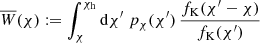
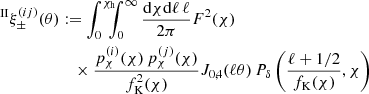
The shear correlation function with IA terms, Eq. (7), is still linear in the matter power spectrum, hence a deprojection of ξ±(ij)(θ) into Pδ(k, z) is, as in S12, principally possible through linear minimum-variance estimators that depend only on the background fiducial cosmology, source distributions, and IA parameters. On the practical side, however, the deprojection is hampered by broad, partly similar lensing kernels, the relatively low signal-to-noise ratio, and a confined θ-range, rendering the estimators ill-conditioned (or singular). They are also biased when ignoring the θ-confinement which amounts to setting ξ(ij)(θ)≡0 outside the θ range (Section 7 in Schneider et al. 2002). Similar to S12, we addressed these practicalities by boundary conditions Pδ(k, z)≥0 through priors in the framework of a Bayesian analysis, at most a couple of redshift bins for Pδ(k, z), and by varying Pδ(k, z) within a confined region in (k, z)-space only, assuming a reference power, Pδfid(k, z), otherwise. Additionally, it is sensible to constrain the relative deviations fδ(k, z):=Pδ(k, z)/Pδfid(k, z) instead of Pδ(k, z) directly: Most of the evolution is probably already accounted for in Pδfid(k, z), and a slowly changing fδ(k, z) within a broad z-bin is a reasonable quantity to be averaged. We describe the implementation details below.
In our set-up, the fδ(k, z) shall be constant within cells of a regular mesh of (Nk + 1)×(Nz + 1) mesh points (km, χn), where km < km + 1, zn < zn + 1, and χn := χ(zn); the intervals [z1, zNz + 1) and [k1, kNk + 1) define the z- and k-ranges where the power spectrum may differ from Pδfid(k, z), here for  and z ∈ [0, 2). The matter power spectrum for Eq. (7) thus equals
![Mathematical equation: $$ \begin{aligned} P_\delta (k,\chi )&= P^\mathrm{fid}_\delta (k,\chi )\left( 1+\sum _{n,m = 1}^{N_z,N_k} H_{mn}(k,\chi )\left[f_{\delta ,mn}-1\right]\right)\;, \end{aligned} $$](/articles/aa/full_html/2025/06/aa54017-25/aa54017-25-eq20.gif) (12)
(12)
where
 (13)
(13)
is a two-dimensional top-hat function. The average of fδ(k, z) within a cell (or band) is denoted by the coefficient fδ, mn. The mesh in k-direction is equi-spaced on a log-scale, Δk = k Nk−1 ln(kNk + 1/k1), while the z-direction uses for one variant zn ∈ {0, 0.3, 0.6, 2}, for Nz = 3, and zn ∈ {0, 2} in other variant with one wide bin, Nz = 1, when averaging fδ(k, z) over the entire redshift range. The number of k-bins is always Nk = 20.
Using this fδ, mn-representation of Pδ(k, z), Eq. (7) is now recast into
 (14)
(14)
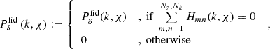
for the projection matrix
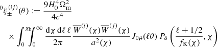
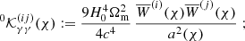
![Mathematical equation: $$ \begin{aligned} X^{(ij)}_\pm (\theta ;m,n)&:=\frac{1}{2\pi \,\theta ^2}\, \int _{\chi _n}^{\chi _{n+1}}\mathrm{d}\chi \; \left(^0\mathcal{K}^{(ij)}_{\gamma \gamma }(\chi )+ ^\mathrm{II}\mathcal{K}^{(ij)}_{\gamma \gamma }(\chi )+ ^\mathrm{GI}\mathcal{K}^{(ij)}_{\gamma \gamma }(\chi )\right)\nonumber \\&\quad \times \int \limits _{k_m f_{\rm K}(\chi )\theta }^{k_{m+1}f_{\rm K}(\chi )\theta }\mathrm{d} s\,s\, J_{0,4}(s)\,P^\mathrm{fid}_\delta \!\left(k[s,\chi ,\theta ],\chi \right)\;, \end{aligned} $$](/articles/aa/full_html/2025/06/aa54017-25/aa54017-25-eq23.gif) (15)
(15)
the integral kernels
 (16)
(16)
 (17)
(17)
 (18)
(18)
and a constant offset
![Mathematical equation: $$ \begin{aligned} \xi _{\pm ,\mathrm {fid}}^{(ij)}(\theta )&:=\frac{1}{2\pi \,\theta ^2}\,\int _{0}^{\chi _{\rm h}}\mathrm{d}\chi \left(^0\mathcal{K}^{(ij)}_{\gamma \gamma }(\chi )+ ^\mathrm{II}\mathcal{K}^{(ij)}_{\gamma \gamma }(\chi )+ ^\mathrm{GI}\mathcal{K}^{(ij)}_{\gamma \gamma }(\chi )\right)\nonumber \\&\quad \times \int \limits _{0}^{\infty }\mathrm{d} s\,s\, J_{0,4}(s)\, {P}^\mathrm{fid}_\delta \left(k[s,\chi ,\theta ],\chi \right) \end{aligned} $$](/articles/aa/full_html/2025/06/aa54017-25/aa54017-25-eq27.gif) (19)
(19)
from (k, z) regions that are unaffected by the choice of fδ, mn. The offset employs the definition
 (20)
(20)
and the foregoing equations abbreviate ![Mathematical equation: $ k[s,\chi,\theta]:=\frac{s+\theta/2}{f_{\mathrm{K}}(\chi)\theta} $](/articles/aa/full_html/2025/06/aa54017-25/aa54017-25-eq29.gif) .
.
Our code computed the projection matrix X±(ij)(θ; m, n) once for a series of θ-bins, enabling a quick prediction of ξ±(ij)(θ) when Monte Carlo sampling the posterior PDF of fδ, mn. An efficient way to numerically calculate X±(ij)(θ; m, n) and  is given in Appendix A of S12, albeit with the little modification (2fK[χ])−1 in what is now
 ![Mathematical equation: $ \bar{k}_j:=(2f_{\mathrm{K}}[\chi])^{-1}+(\hat{k}_j+\hat{k}_{j+1})/2 $](/articles/aa/full_html/2025/06/aa54017-25/aa54017-25-eq31.gif) due to the extended hybrid Limber approximation adopted here. As further practical footnote on code implementation, we performed the above integrals with integration variable a instead of χ, as well as pz(z) instead of pχ(χ), for which the following transformations are notable, given a general function g(χ) and H(a) = : H0 E(a),
due to the extended hybrid Limber approximation adopted here. As further practical footnote on code implementation, we performed the above integrals with integration variable a instead of χ, as well as pz(z) instead of pχ(χ), for which the following transformations are notable, given a general function g(χ) and H(a) = : H0 E(a),
![Mathematical equation: $$ \begin{aligned} \int _{\chi _1}^{\chi _2}\mathrm{d}\chi \;g(\chi ) = \frac{c}{H_0}\int _{a_2}^{a_1}\frac{\mathrm{d} a}{a^2\,E(a)}\;g[\chi (a)] \end{aligned} $$](/articles/aa/full_html/2025/06/aa54017-25/aa54017-25-eq32.gif) (21)
(21)
since |dχ/da|=c/(a2H[a]),
![Mathematical equation: $$ \begin{aligned} \int _{\chi _1}^{\chi _2}\mathrm{d}\chi \;p^{(i)}_\chi (\chi )\,g(\chi ) = \int _{a_2}^{a_1}\frac{\mathrm{d} a}{a^2}\;p_z^{(i)}[z(a)]\,g[\chi (a)] \end{aligned} $$](/articles/aa/full_html/2025/06/aa54017-25/aa54017-25-eq33.gif) (22)
(22)
since |dz/dχ|=H(z)/c, and hence
![Mathematical equation: $$ \begin{aligned}&\int _{\chi _1}^{\chi _2}\mathrm{d}\chi \;p^{(i)}_\chi (\chi )\,p^{(j)}_\chi (\chi )\,g(\chi )\nonumber \\&\quad =\frac{H_0}{c}\, \int _{a_2}^{a_1}\frac{\mathrm{d} a\;E(a)}{a^2}\,p_z^{(i)}[z(a)]\,p_z^{(j)}[z(a)]\,g[\chi (a)]\;. \end{aligned} $$](/articles/aa/full_html/2025/06/aa54017-25/aa54017-25-eq34.gif) (23)
(23)
When integrating over pz(i)(z), we adopted histograms with top-hat functions, without interpolation, exactly as indicated in Fig. 1. The very first bin, left-aligned towards z = 0, has pz(i)(z) = 0. Probably obvious through these integrals and the pre-factors in Eqs. (8)–(10), the projections of Pδ(k, z) into ξ(ij)(θ) are independent of H0 as long as [k]=h Mpc−1 (comoving), whereas the ξ±(ij)(θ) scale with Ωm2 since F(χ)∝Ωm.
3. Bayesian inference of the three-dimensional matter power-spectrum
With the linear relation between the three-dimensional (3D) power spectrum and the two-point shear correlation functions described, we now outline the statistical model and the numerical sampler for the posterior probability density of fδ, mn within a Bayesian framework (e.g., Gelman et al. 2003, for a review). In comparison to S12, our updated methodology introduces the Tikhonov regularisation as Bayesian prior, in effect inferring a k-smoothed power spectrum, and a Hamiltonian MCMC for improved computational speed for Nz × Nk ∼ 60 model variables.
3.1. Statistical model
The statistical model of fδ, mn employs a compact notation for the tomographic data, model variables and parameters, all presented here. The vector of model variables π = (fδ, mn|1≤n≤Nz,1≤m≤Nk) compiles the bin-averaged fδ(k, z) on a (Nk + 1)×(Nz + 1) mesh, and the data vector d contains the binned ξ±(ij)(θk) for a sequence of Nθ = 9 angular separations, θk. Equation (14) predicts the components of d for a given (flat) background cosmology, IA parameters, and source redshift distributions, altogether compressed into q = {Ωm, AIA, pz(1)(z),…,pz(5)(z)} hereafter. The prediction is denoted by the model vector  with elements arranged in the same order as those in d, using the projection matrix Xq which contains the coefficients X±(ij)(θ; m, n) for fixed q. The elements of
  are the offsets
  , also for fixed projection parameters q. The statistical information on π is expressed by the Bayesian posterior PDF of π conditional on d,
 (24)
(24)
adopting a Gaussian likelihood
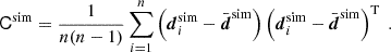
![Mathematical equation: $$ \begin{aligned} -2\,\ln {\mathcal{L}_{\boldsymbol{q}}(\boldsymbol{d}|\boldsymbol{\pi })}= \left[\boldsymbol{d}-\boldsymbol{m}(\boldsymbol{\pi },\boldsymbol{q})\right]^\mathrm{T}\mathsf C ^{-1} \left[\boldsymbol{d}-\boldsymbol{m}(\boldsymbol{\pi },\boldsymbol{q})\right] \end{aligned} $$](/articles/aa/full_html/2025/06/aa54017-25/aa54017-25-eq39.gif) (25)
(25)
with error covariance C of the measurement d, and two prior probability densities, Phat(π) and Pτ(π), to regularise the sampling in fδ-parameter space. The normalisation,  , is not of interest for the Monte Carlo sampler, and hence we set
  without impacting the results. We describe the two prior PDFs in the following.
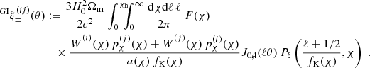
3.2. Tikhonov regularisation prior
The Tikhonov regularisation prior, Pτ(π), greatly improves the constraints, pruning implausible solutions for fδ, mn. This is necessary because the combination of heavy smoothing and added noise in ξ±(ij)(θ) has the unpleasant side-effect of producing strong oscillations, correlated errors, in fδ(k, z) when inverting the tomographic signal. Similar to 3D-lensing mass reconstructions (Hu & Keeton 2002), the oscillations are reduced by applying regularisation conditions. To this effect, the Tikhonov regularisation down-weights oscillating fδ(k, z), preferring solutions of fδ, mn smoothed in k-direction,
 (26)
(26)
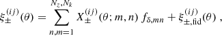
At the same time, no prior constraints are imposed on the overall amplitude of fδ, mn or the difference signal between z-bins because only signal differences from the same z-bin, n, appear inside the prior density. The weight of the prior relative to the data likelihood  is controlled by the Tikhonov parameter τ, demonstrated in Fig. 2 for a simulated analysis with three redshift bins, Nz = 3.
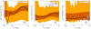 |
Fig. 2. Impact of the Tikhonov regularisation used to suppress oscillating solutions fδ(k, z). Shown are, for a noise-free mock data vector and the KiDS-1000 error covariance, the posterior constraints (68% credible regions) on fδ averaged over the redshift bin Z1 = [0, 0.3] (left), Z2 = [0.3, 0.6] (middle), and Z3 = [0.6, 2] (right) with and without regularisation (dark orange τ = 5.0 with median as dashed line or light orange τ = 0). To boost scale-dependence and evolution, fδ(k, z) is here defined relative to the power spectrum at fixed redshift, probing the relative structure growth since z = 1. The solid line is the median posterior fδ for 100× reduced measurement errors, providing a nearly noise-free reference (noise/100) that averages the growth over the redshift bin while still exhibiting artefacts near the edges. The dotted lines are the theoretical |


This intentionally extreme scenario in Fig. 2 highlights the impact of the regularisation with a truly z-evolving and scale-dependent fδ, mn by choosing a constant reference Pδfid(k, z) for all z-bins: a theory power spectrum at z = 1. Unlike the actual KiDS analysis in Sect. 5, the fδ, mn therefore now quantify the structure growth relative to z = 1. To assess the quality of the reconstruction and our ability to detect the z- and k-dependence of fδ, mn, we analysed a mock vector d = m(π, q) with parameters in Table 1 and KiDS-1000-like noise, C, yielding posterior 68% credible regions with regularisation (τ = 5, dark orange) and without (τ = 0, light orange). The figure compares these credible regions to virtually noise-free data, unaffected by the Tikhonov regularisation, depicted as solid lines (“noise/100”). The solid lines are, to account for the z-weighting of fδ(k, z) in a reconstruction, the posterior medians for a data vector with unrealistically high signal-to-noise ratio (S/N) of C′ = 10−4 × C as error covariance and no Tikhonov regularisation. But even for such high S/N data, artefacts appear towards large scales, close to k ∼ 0.02 h Mpc−1, and at the high-k end, near k ∼ 10 h Mpc−1, thus towards k where the tomographic data poorly constrain the power spectrum. To mitigate these artefacts, the additional dotted lines depict for each z-bin a theoretical  at one specific redshift,
  , that matches the solid lines most closely, and which shall be the ‘true’ average fδ, mn for this experiment. Undoubtedly, a Tikhonov prior, τ = 5, substantially reduces the statistical uncertainty in the reconstruction (sizes of credible regions for τ = 0 versus τ = 5). On the downside, however, the regularisation might be overly restrictive by straightening out oscillations actually present in the data, as already partly present for τ = 5 (dotted lines versus dashed lines, the posterior median). By running more tests with different τ, not shown here, we consider τ = 5 a good compromise that catches gradual trends with k while improving the precision in the reconstruction, as in the left panel. We reiterate that the degree of evolution and scale-dependence in this test, due to the static reference power spectrum, is extreme compared to what is expected in the KiDS-1000 analysis. If the reference is close to the true matter power at all z, fδ, mn will be close to unity.
Parameters of the reference power spectrum, Pδfid(k, z), and the projection parameters (lensing kernel, IA) used to infer fδ(k, z) = Pδ(k, z)/Pδfid(k, z).
A cruder alternative to Tikhonov filtering (τ = 0) for smoothing the reconstruction involves drastically reducing the number of k-bins, such as to Nk = 5. This approach, however, significantly blurs fδ(k, z) and their scale-dependent features, effectively smoothing it to the fixed size of the larger k-bins, resulting in a distinctly lower resolution compared to Tikhonov filtering. In contrast, Tikhonov filtering applies adaptive smoothing, using smaller smoothing kernels where the S/N is higher and broader kernels elsewhere. This method’s resolution is limited only by the size of the numerous, smaller k-bins, for which we chose Nk = 20.
3.3. Positivity priors
Already applied for Fig. 2, we restricted valid solutions to positive fδ, mn (since Pδ(k, z)≥0), by using uniform, top-hat prior PDFs for ![Mathematical equation: $ f_{\delta,mn}\in[0,f_{\delta,\rm max}] $](/articles/aa/full_html/2025/06/aa54017-25/aa54017-25-eq49.gif) ,
,
![Mathematical equation: $$ \begin{aligned}&-\sigma _{\rm f}^2\,\ln {P_{\rm hat}(\boldsymbol{\pi })}= \sum _{n,m = 1}^{N_z,N_k}\left( f_{\delta ,mn}^2\,\mathrm{H} \left[-f_{\delta ,mn}\right]\right.\nonumber \\&\quad \left. +\left[f_{\delta ,mn}-f_{\delta ,\mathrm {max}}\right]^2\,\mathrm{H} \left[f_{\delta ,mn}-f_{\delta ,\mathrm {max}}\right] \right)\;, \end{aligned} $$](/articles/aa/full_html/2025/06/aa54017-25/aa54017-25-eq50.gif) (27)
(27)
where H(x) is the Heaviside step function. Enforcing positive solutions for the matter power spectrum is beneficial in reducing both the statistical errors and oscillations in the reconstruction, as already reported in S12. The positivity priors adopt wide intervals,  , compared to expected values of fδ, mn ∼ 1. In addition, for numerical convenience, the top-hat priors have soft edges, σf = 10−2, to relax issues with low acceptance rates and undefined gradients in the Monte Carlo sampler of P(π|d) near the edges.
3.4. Monte Carlo sampler
For sampling the posterior PDF, Eq. (24), we applied a MCMC technique that represents P(π|d) by nmcmc = 104 points (πi, wi) with statistical weights, wi, for given projection parameters q. The MCMC sampler is a Hamiltonian Monte Carlo algorithm, known to be efficient even for high-dimensional models (Nz × Nk ∼ 60) by proposing new, quickly decorrelating sampling points with high acceptance rate (Gelman et al. 2003). The sampler, however, requires as input the gradient  and the gradient of the logarithmic prior densities – all easily available in our case, foremost because of the linear projection
  . We demonstrate the appropriate sampler performance in Appendix A and provide more implementation details there. Due to the efficient decorrelation of the MCMCs, we shortened the burn-in phase for the KiDS-1000 analysis, nburnin = 5 × 10³, in comparison to Appendix A, and used shorter chain lengths because of the subsequent merger of many chains when marginalising over q, outlined in the next section.
3.5. Marginal errors including uncertainties in IA and lensing kernel parameters
The parameters for the lensing kernel and IA are neither exactly known nor intended to be constrained by our shear data. Therefore, to account for their uncertainties in fδ, mn, the analysis combines many chains with nruns = 500 realisations of q drawn from a baseline error model. The error baseline adopted a flat cosmology, ΩΛ = 1 − Ωm, and a random sample of the posterior joint distribution of (Ωm, AIA) from the recent 3 × 2 pt cosmological analysis in Heymans et al. (2021); their marginal errors are  and
and  (68% CI). The 3 × 2 pt experiment combines the KiDS-1000 cosmic shear constraints with those from galaxy-galaxy lensing and, importantly, the galaxy clustering in the partly overlapping, spectroscopic surveys of both the 2-degree Field Lensing Survey and the Baryon Oscillation Spectroscopic Survey (Blake et al. 2016; Alam et al. 2015) to break the σ8 − Ωm degeneracy in the shear data. This substantially reduces the uncertainty of Ωm in the lensing kernel while, at the same time, using only z ≲ 1 data. Furthermore, for error realisations of the source distributions, we shift the histograms in Fig. 1 according to pz(i)(z)→pz(i)(z + δzi), for random draws of δzi confined by the error model in Hildebrandt et al. (2021), their Figure 6 and Table 3; the root-mean-square (RMS) error of δzi is σzi ≈ 1.3 × 10⁻² for all tomographic bins, except for i = 3 where σzi = 2 × 10⁻². Within this Monte Carlo process, we fixed the reference Pδfid(k, z) for all chains to that in Table 1 to avoid conflicting definitions of fδ, mn while varying Ωm.
After all MCMCs with randomised lensing kernels and IA parameters were available, we combined the nruns runs by selecting from each chain j a number of nmerge = 103 sampling points πij with probability wij/∑iwij. Selected points were put back into the sample j, to be possibly selected again. By doing so, the selected nmerge points sample the posterior of chain j when equally weighted. Mixing the MCMC points from all nrun chains for the final Monte Carlo sample then contains nmerge × nruns = 5 × 10⁵, equally weighted sampling points πij of the marginalised posterior distribution of fδ, mn.
4. Data
We used the public data from the fourth Data Release (DR4) of the Kilo-Degree Survey (Kuijken et al. 2019), commonly referred to as the KiDS-1000 data1. The images underlying the data were taken by the high-quality VST-OmegaCAM (Kuijken 2011), covering a total area of about 1006 deg2 in four optical filters (ugri). After masking, the effective area of the KiDS-1000 data is 777.4 deg2. Its overlap with the VIKING survey (Vista Kilo-degree Infrared Galaxy survey, Edge et al. 2013), which observes in five near-infrared bands, ZYJHKs, allows a better control over redshift uncertainties (Hildebrandt et al. 2021).
4.1. Source catalogue
The following summarises the production of the shear catalogue, carried out by the KiDS-1000 Consortium. The images were processed using the THELI (Erben et al. 2005) and ASTRO-WISE (Begeman et al. 2013) pipelines, source ellipticities were estimated by lensfit (Miller et al. 2013; Fenech Conti et al. 2017). Based on the nine-band catalogue, individual photometric redshift estimates, zB, were obtained using BPZ (Benítez 2000), dividing the sources into five tomographic bins (Fig. 1).
To calibrate the redshift distribution of each tomographic bin, Wright et al. (2020a) construct a self-organising map (SOM) linking the nine-band photometry of the sources to a representative spectroscopic sample. Galaxies without matching spectroscopic counterparts, or for which the zB are catastrophically different from the redshift of the matched spectroscopic sample, are expunged from the catalogue (Wright et al. 2020b). The mean and the scatter, δzi, on the bias of the means of the pz(i)(z), estimated by the SOM, are numerically estimated using a suite of KiDS-like mock observations (Hildebrandt et al. 2021)2. The resulting ‘gold sample’ contains ∼2.1 × 10⁷ sources with well-calibrated photometric redshift distributions; Giblin et al. (2021) gives more details. Table 2 in the Appendix summarises the main parameters relevant for our analysis. Cosmological parameter constraints from the KiDS-1000 tomographic data, with the methodology in Joachimi et al. (2021), are presented in Asgari et al. (2021), exclusively using cosmic shear, in Heymans et al. (2021), using 3 × 2pt data, and in Tröster et al. (2021), for a beyond ΛCDM analysis using 3 × 2pt data.
Overview of the KiDS-1000 ‘gold sample’
4.2. Data vector and covariance of measurement noise
Based on the tomographic shear data, the KiDS-1000 DR4 provides estimates of the binned shear correlation function, ξ±(ij)(θ), for every combination of tomographic bins, (ij), employing the popular computer software TreeCorr (Jarvis et al. 2004; Jarvis 2015). We used these data without modification. For the ξ± estimator details, we refer to Asgari et al. (2021), Section 2.1 and Appendix C, and only note that we analysed the ξ±(ij)(θ) binned into Nθ = 9 angular log-bins for the range  –300′. Another notable technical detail, the data vector for the DR4 was obtained by rebinning a previously finely binned vector, instead of rerunning TreeCorr. Further, Asgari et al. (2021) exclude scales smaller than 4′ for ξ− due to high systematic uncertainties in the theoretical matter power-spectrum on small scales, whereas our model-free measurement of Pδ(k, z) included scales down to
  .
.
The covariance matrix of noise, C in Eq. (25), for the estimator of ξ±(ij)(θ) used the analytical model by Joachimi et al. (2021), Appendix E. This model accounts for the intrinsic shape scatter of sources, for both Gaussian and non-Gaussian cosmic variance, mostly relevant towards larger angular scales, for the super-sample covariance due to fluctuation modes greater than the survey footprint, and for the calibration uncertainty in the multiplicative shear bias. As for ξ±(ij)(θ), the covariance matrix is part of the package of additional DR4 data products.
4.3. Systematic shear error
In addition to intrinsic alignments, a residual systematic error in the shear signal through the data reduction or the instrument may also be potentially present in ξ±(ij). Detecting B-modes in the shear field, specifically  as defined in Eq. (2), is considered a strong indicator of systematic errors, because B-modes generated by weak gravitational lensing are negligible. Clearly separating B-modes from E-modes in a ξ±(ij) with finite support is, however, unfeasible, but other related statistics are known to separate both modes (and ambiguous modes), most prominently COSEBIs (Schneider et al. 2010). For KiDS-1000, logarithmic COSEBIs capturing scales ℓ ≲ 103 do not indicate B-modes on a 95% confidence level (Asgari et al. 2021; Giblin et al. 2021), several other tests for systematic errors are negative, and the cosmological analysis with the E-mode COSEBIs yields results consistent with a ξ±(ij) analysis. Therefore, a significant bias of parameters in a cosmological analysis due to a systematic shear error is unlikely.
Notably, however, the COSEBIs cosmological analysis alone is insensitive to small angular scales of ℓ ∼ 104, included in our analysis through θ ≲ 4′ in ξ−(ij). In addition, even a small systematic shear error in ξ±(ij) might cause artificial deviations of Pδ(k, z) from the reference Pδfid(k, z), i.e., fδ, mn ≠ 1, if the error is of the order of the difference signal between the measured ξ±(ij) and the expected signal in Eq. (14) for fδ, mn ≡ 1. The 1σ–2σ window left open for B-modes by the logarithmic COSEBIs therefore leaves the possibility that deviations in KiDS-1000 might partly be related to a systematic shear error in the data. We return to this caveat in Sect. 6.
5. Results
This section reports our results for the relative power spectrum, fδ, mn, in two variants: an entirely average, non-evolving scenario (one broad redshift bin) and an evolving scenario with three independent redshift bins. In addition, we verified our pipeline with results from a mock analysis based on ray-traced N-body data in an entirely ΛCDM framework.
5.1. Reference ΛCDM matter power-spectrum
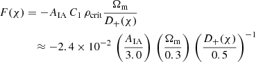
For the KiDS-1000 analysis presented here, the reference power spectrum, Pδfid(k, z), is a revised halofit model with the parameters in Table 1 (Takahashi et al. 2012; Smith et al. 2003). These parameters are maximum-posterior values taken from Table C.1 (3 × 2 pt, joint) in Heymans et al. (2021) with one modification: the value for σ8 was lowered from 0.76 to 0.72 to achieve the best fit to KiDS-1000 data that averages out to ⟨fδ, mn⟩mn ≈ 1 over all m and n (the next Sect. 5.2 provides more details). This σ8 reduction is presumably required because the Pδ(k, z) model in Heymans et al. (2021) includes neutrino suppression and baryonic feedback, missing here, and is, even without neutrinos and baryons, already systematically lower by roughly 5%–10% within k ≈ 0.1–10 h Mpc−1 compared to halofit. We refer to Section 4 in Mead et al. (2015) for a discussion on the latter aspect, and reiterate that our Pδfid(k, z) choice is arbitrary – in our analysis, a purely ΛCDM model that matches the KiDS-1000 data. The results for fδ(k, z) in the following sections consequently probe the deviations of the true Pδ(k, z) relative to the best-fitting ΛCDM reference.
5.2. Evidence for deviation from reference
A hypothesis test against null models with constant  , for all m and n, and fixed projection parameters q shows that the KiDS-1000 data support deviations from the reference power spectrum in either k or z, shown by the results in Fig. 3. For each
  on the x-axis in this figure, 105 noise realisations of dnull were used in the null model to predict the cumulative distribution C[tnull] of the test statistic
  . The y-axis shows the probability, p := C[td], that the null model exceeds the
  in the actual data (solid line) or, for verification, in random null-model data (dashed line). Starting with the reference power spectrum (
 ), as indicated by the yellow vertical line, the KiDS-1000 data have p = 0.012 and the verification data p = 0.78. Therefore, while the verification data are well within the expectation of the null hypothesis, the KiDS-1000 data are inconsistent with reference model on a 1 − p = 98.8% confidence level. Varying
  , however, would not improve the test result because the KiDS-1000 curve already peaks at
  : the reference power spectrum, Pδfid(k, z), is the best fit out of a family of models with constant fδ, mn. The only way to improve the fit would be to make fδ, mn varying with either scale, k (this means m), or redshift, z (this means n).
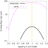 |
Fig. 3. Test of data against a null model with identical |


In fact, the peak at  was our deliberate choice for KiDS-1000, achieved by lowering σ8 for Pδfid(k, z) to 0.72 compared to the best-fitting value of 0.78 in Heymans et al. (2021) in order to move the peak from
  to its final location
  . This way, the fδ, mn in our data are normalised to the average ⟨fδ, mn⟩mn ≈ 1. The failed null test still stands, however, and is evidence for the existence of a better fit by introducing either a k- or z-dependence of fδ, mn, or both. This is explored in the following two more complex scenarios.
5.3. Average deviations over full redshift range
The first scenario introduces a k-dependence for fδ, mn without redshift evolution (Nz = 1), reported with 68% CI about the median in the left panel of Fig. 4. In other words, the redshift evolution of Pδ(k, z) is assumed to be that of the reference power spectrum. Towards non-linear scales k ≳ 0.1 h Mpc−1, there is no indication for a deviation from the reference exceeding the 68% CI, in particular the suppression of power does not fall below fδ ≈ 0.8, nor do the data support a boost of power beyond fδ ≈ 1.2. Towards linear scales, below k ≈ 0.1 h Mpc−1, is a slight, yet insignificant, rise towards fδ ≈ 1.5. This might be a sign that halofit with higher σ8 provides a slightly better fit on linear scales. Yet, on average, variations relative to Pδfid(k, z) stay within about 20% (68% CI) down to k ∼ 10 h Mpc−1.
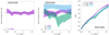 |
Fig. 4. Reconstructed matter power spectrum in KiDS-1000 for τ = 5.0 and Nk = 20 in three variants. The errors marginalise over uncertainties in the lensing kernel and IA. Shown are the posterior 68% CI about the median (lines). Left panel: Transfer function fδ(k, z) averaged over the entire redshift range Z1 = [0, 2] and relative to the reference, Pδfid(k, z), with parameters listed in Table 1. Middle panel: Same as the left panel, but for three independent transfer functions averaged separately within the ranges Z1 = [0, 0.3], Z2 = [0.3, 0.6], and Z3 = [0.6, 2]. Right panel: Dimensionless power spectrum, Δ2(k, z) = 4π k3Pδ(k, z) = 4π k3 fδ(k, z) Pδfid(k, z), interpolated to the centres of three redshift bins Z1, Z2, and Z3. |
5.4. Deviations for three separate redshift bins
For more insight in a possible z-evolving fδ in the second scenario, we probed the average fδ(k, z) inside three separate redshift bins, Z1 = [0, 0.3], Z2 = [0.3, 0.6], and Z3 = [0.6, 2]. Their marginalised posterior constraints (68% CI about the median) are plotted as three credible regions in the middle panel of Fig. 4, one region for each redshift bin. The lowest bin, Z1, is fully consistent with fδ = 1, on k-average fδ = 1.15 ± 0.28, while the middle bin, Z2, on average fδ = 0.57 ± 0.27, indicates a power suppression, reaching the depth fδ = 0.3 ± 0.2 at k ∼ 0.5 h Mpc−1, and the highest bin, Z3, overall prefers a boosted power of fδ = 2.22 ± 0.81. The signal suppression in the middle redshift bin and the boost in the highest bin cancel each other when averaging fδ over the whole redshift range, resulting in the fδ = 0.99 ± 0.20 in the left panel.
The close description of the ξ±(ij)(θ) data points by the flexible fδ model is illustrated by the posterior predictive of the model in Fig. B.1 (Appendix). Shown in the various panels are our KiDS-1000 data points (black with 1σ errors bars) for θ ξ−(ij)(θ) (lower left panels) and θ ξ+(ij)(θ) (upper right panels) in comparison to the posterior model constraints (68% and 95% CIs in dark and light blue). The CIs in this plot do not marginalise over q; however, this has an effect of less than 10%. The red line corresponds to the ΛCDM reference model, this means fδ, mn ≡ 1, obtained from a best fit of σ8 to the data points (Sect. 5.1). Allowing for deviations fδ, mn ≠ 1 in the three separate redshift bins Z1 to Z3 moves the CIs relative to the reference, thereby improving the fit, although the reference still stays within the 95% CI, as, for instance, for ξ±(55)(θ). Whilst an overall good match to the (correlated) data points, a conflict with the model is probably present for ξ+(22)(θ), and perhaps in ξ+(12)(θ) to ξ+(15)(θ), where the data prefer a higher amplitude than the model fitting all tomographic bins. Figure A.4 shows a similar plot with verification data, based on the reference model, as comparison. A higher value of  , as indicated by the green line for the N-body verification data (without IA, Sect. 5.5), would account for the higher ξ+(1j)-amplitude but, on the other hand, is rejected by the data due to mismatches at higher redshift (e.g., ξ+(35) or ξ+(45)). This might indicate spurious systematic errors in the low-z bins, discussed in Sect. 6.
Expressed in terms of the actual power spectrum,  , interpolated to the z-bin centres,
  , the diverse redshift evolution of fδ(k, z) in the KiDS-1000 data translates into a suppression of non-linear structure growth between 0.3 ≲ z ≲ 2. Namely, the
  matter power spectrum in the right panel of Fig. 4 (magenta) has clearly more power than the two higher redshift bins (green for
  and cyan for
  ) for k ≳ 0.1 h Mpc−1, while the two other power spectra are consistent with each other, maybe with the green rising over cyan near k = 10 h Mpc−1. Consequently, with cyan and green being moved closer to each other, there is for k ≳ 0.1 h Mpc−1 less structure growth detected between
  –1.3 than in the reference ΛCDM cosmology but, conversely, more between
  –0.45, pulling back the low-z bin to the reference power spectrum.
It is noteworthy that the statistical errors of fδ, mn and hence Δ2(k, z) are correlated, best visualised by the correlation matrix in Fig. 5. Each pixel in the correlation matrix encodes the Pearson correlation coefficient, r, between two k-bins, either from same or from different z-bins. The matrix is organised in Nk × Nk blocks, where k increases from left to right and top to bottom. The three blocks on the diagonal, bottom left to top right (lowest z to highest z), are correlations within the same redshift bin, and the six off-diagonal blocks are cross-correlations between distinct z-bins. The enhancement of correlations within the blocks, making them stick out as tiles in a 3 × 3 mosaic, is a side-effect of the Tikhonov regularisation smoothing the fδ, mn along the k-axis. Correlations are high for adjacent k-bins in the same z-bin, r ≈ 0.4–0.8, especially in the highest z-bin (top right), but quickly drop off with distance on the k-scale. Adjacent k-bins are also statistically dependent when from adjacent z-bins, albeit now anti-correlated with typically r ≈ −0.4 to −0.1. Not shown is the correlation matrix for a Nz = 1 reconstruction, left panel in Fig. 4, to save space; it is essentially a diagonal matrix where adjacent k-bins have |r|≲0.1, except at the lower and upper boundary of the k-range where r ≈ 0.5–0.6.
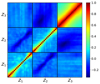 |
Fig. 5. Correlation matrix of fδ, mn errors for the KiDS-1000 analysis with three redshift bins, corresponding to the middle and right panels in Fig. 4. The three blocks on the diagonal from bottom left to top right are the correlation matrices for the z-bins Z1 = [0, 0.3], Z2 = [0.3, 0.6], Z3 = [0.6, 2], respectively; off-diagonal blocks show correlations between distinct z-bins; pixels within the 20 × 20 blocks are correlations between the k-bins, ascending from left to right inside a block. |
5.5. Verification test with ray-traced mock data
To add more realism to the code verification than in Appendix A, especially with respect to the fδ result for Nz = 3, we performed a more stringent test with N-body ray-traced data (Takahashi et al. 2017). As in Burger et al. (2024), we subdivided the 108 full-sky shear fields from the simulated data according to the KiDS-1000 sky area and, for each tomographic bin, combined 30 shear grids for ascending source redshifts according to the redshift distributions in Fig. 1. This yields an ensemble of n = 1944 mock KiDS-1000 surveys. From these, source positions were picked to match the angular positions, shear weights, and shape noise to the measured counterparts in the public KiDS-1000 ellipticity catalogue (Giblin et al. 2021). In contrast to Appendix A, however, intrinsic alignments of sources are not included here, thus AIA = 0. Similar to the actual KiDS-1000 data vector, we used TreeCorr to compute ξ±(ij)(θ) from the mock shear catalogues.
Driven first by the question whether our code can recover fδ(k, z) = 1 from a simulated (unrealistically) high S/N data vector when using exactly the same cosmological parameters as in the simulation, we averaged all n realisations of the data vector, denoted by  , and used the individual realisations, disim, to estimate the (standard) error covariance of
  ,
,
 (28)
(28)
This covariance matrix was turned into an unbiased estimator of the inverse covariance using Hartlap et al. (2007). The average  and Csim are basically a single measurement in a hypothetical survey with n times the angular area than KiDS-1000, albeit underestimating the cosmic variance error. For an initial inspection, the solid green lines SIM-THS17 in Fig. B.1 (Appendix) compares
  to the real KiDS-1000 data (black data points with error bars): The simulated tomography correlations are mostly within the 1σ noise scatter of the KiDS-1000 data points, yet exhibit systematically more signal compared to the reference model (red lines) by occasionally exceeding the 95% CIs, probably due to the higher fluctuation amplitude, S8 ≈ 0.791 in the simulation compared to S8 ≈ 0.765 in KiDS-1000, and, less relevantly, the missing IA terms in the simulation. Now, using
  and Csim as input, the data points in the top panel of Fig. 6 show the code results for fδ(k, z) in three redshift bins. To test the code’s ability to recover the power spectrum in the simulation, fδ(k, z) = 1, the reference Pδfid(k, z) was set here to the same cosmological parameters as in the N-body data, namely Ωm = 0.279, ΩΛ = 1 − Ωm, Ωb = 0.046, h = 0.7, ns = 0.97, and σ8 = 0.82. Since the lensing kernel is exactly known in this experiment, no marginalisation of q was done. We find the following.
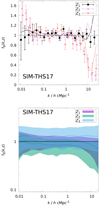 |
Fig. 6. Verification test of the analysis code for fδ(k, z) using: an N-body simulated data vector, averaged over n = 1944 realisations of the KiDS-1000 data without IA; the code and data set-up for the KiDS-1000 analysis has Nk = 20 k-bins and three redshift bins Z1 = [0, 0.3], Z2 = [0.3, 0.6], and Z3 = [0.6, 2]. The reference power, Pδfid(k, z), is here identical to the cosmology of the simulation (Takahashi et al. 2017). The errors (68% CI) do not marginalise over a projection kernel uncertainty. Top panel: Simulated covariance of the average data, comprising n times the area of KiDS-1000. Deviations from the expected fδ(k, z) = 1 towards higher z and k ≳ 1 h Mpc−1 are related to the finite grid pixel size in the simulation (pixelation bias). The lines are additional reconstructions using noise-free data, based on Eq. (8) and halofit without pixelation bias. Bottom panel: Same as top panel, but with statistical errors as in a single KiDS-1000 survey. |
The reconstructed power spectrum in Fig. 6, top panel, for the lowest redshift bin (filled squares) is overall consistent with fδ, mn = 1 for the range k = 0.01 − 20 h Mpc−1 within the 68% CI, indicated by the error bars. But two significant deviations emerge: first, in the higher redshift bins beyond k ≈ 5 h Mpc−1, and, second, smaller deviations around 0.01 h Mpc−1. The high-k suppression of the signal is a real feature in the simulation data due to the pixelated shear grids of the simulation (pixel size  ), significantly biasing low the values for ξ−(ij) for θ ≲ 5′. The lowest redshift bin is presumably also affected, but scales of a few arcmins correspond here to a characteristic k too high to be visible in the plot: the typical wave number, keff = 2π/(fK(χd) θ1′), of an angular scale θ1′ = 1′ on a lens plane at distance χd corresponds to
  for lens planes located at the centres of the bins Z1, Z2, and Z3, respectively. The additional lines in the plot support the idea of a pixelation bias: they are reconstructions of noise-free data, based on the simple Limber-Kaiser projection in Eq. (8) – crucially, not showing the systematic signal drop for Z2, or for Z3 around k = 1 h Mpc−1. Instead, however, the lines exhibit artefacts as zig-zag oscillations of amplitude Δfδ ≈ 0.1, strongly increasing towards the edges of the plotted k-range and probably related to the limitations of the deprojection method (Sect. 3.1). The artefacts are partly mirrored in the data point scatter and overlap with the pixelation bias for Z3 (yet not for Z2) at large k.
The second, weaker ∼1.5σ–2σ deviations appear around k = 0.01 h Mpc−1 for Z2 and Z3. They, too, are probably to some extend present in the N-body data: Figure 19 in Takahashi et al. (2017) report a 10% deviation from halofit near k = 0.01 h Mpc−1. Nevertheless, we doubt that this explains the full effect and point out that the plots compare an average data vector in a simulation of finite volume, still subject to noise, to the cosmic average. Especially on large scales, cosmic variance noise is relevant and under-estimated in Csim. In addition, the noise-free data (solid lines) suggest some excess signal on large scales due to edge artefacts. In summary, the bottom panel of Fig. 6 is an excellent reconstruction of the relative power with Δfδ ≈ 0.1 accuracy, or better, for k ≲ 10 h Mpc−1 and z ≲ 1.
Another inference of fδ(k, z) with the simulated data is shown in the bottom panel of Fig. 6 – this time for a KiDS-1000-like error covariance, n × Csim. By using the average  as input, the (essentially linear) reconstruction in the figure represents the ensemble mean of fδ(k, z) posteriors in three redshift bins. In this average reconstruction, the posterior errors are similar to the ones in the KiDS-1000 reconstruction, middle panel of Fig. 4, increasing in size for higher z, although now the fδ, mn are consistent with fδ = 1 throughout (68% CI). The suppression of power by pixelation bias is here fully contained within the statistical errors, only vaguely hinted at in the green Z2 posterior region of Fig. 6, bottom panel, which falls just below fδ = 1 around k = 10 h Mpc−1. Therefore, also for KiDS-1000-like noise levels, the code recovers the correct power spectrum in the N-body data. The highest precision of fδ = 1.00 ± 0.27 is achieved for Z1, the middle bin Z2 has fδ = 0.81 ± 0.31, and Z3fδ = 1.29 ± 0.63 (medians and 68% CIs, no q errors).
For comparison, Fig. A.5 (Appendix) shows an ensemble of reconstructions with individual, 16 randomly chosen disim, illustrating the possible variations in the inferred fδ(k, z). Each panel is a prediction of a KiDS-1000 reconstruction in a ΛCDM scenario. Here, we observe a small tendency of the posterior median in Z3 to be above fδ = 1 and the median in Z2 to be below fδ = 1, despite both having fδ ≈ 1 for k ≲ 5 h Mpc−1. This tendency is also visible in Fig. 6 of average reconstructions, bottom panel, with the posterior median always being above fδ = 1 for Z3, or below for Z2, and probably has two reasons. First, the Z3 bin is poorly constrained, giving a broad marginalised posterior PDF skewed towards higher fδ values, shifting up the centres (posterior medians) of our CIs; this is illustrated by Fig. A.3 in the Appendix. Second, errors in Z2 and Z3 are anti-correlated, preferring a lower value for Z2, if the fδ at similar k in Z3 is scattered upwards. But, on a broad note, one should not expect the maximum of the marginalised PDF to coincide with the maximum of the full posterior (for the non-marginalised parameters) because this requires that the full posterior PDF must obey certain symmetries about its maximum, as, for instance, present in a multivariate Gaussian posterior – excluded here because of our skewed, non-Gaussian marginalised posterior distributions. For increased S/N in the data, however, the long tails of skewed posteriors are suppressed, and the median shift is no longer discernible in the top panel of Fig. 6.
5.6. Impact of uncertainty in IA and lensing kernel
The individual impact by uncertainties in the projection parameters q on the reconstructed fδ, mn is of interest for improving future analyses or to gauge the relevance of errors in the projection kernel. We therefore compare the marginalised fδ, mn errors in the middle panel of Fig. 4 to the statistical errors obtained without marginalisation, or to the errors where all parameters q are fixed but for one that is marginalised over.
Figure 7 shows the results in these different scenarios as function of scale k for three z-bins, indicated in the lower right of each panel; a 100% error is as large as in a scenario where all q uncertainties are marginalised over. The solid black lines use a fixed q without any marginalisation, setting a lower limit for all scenarios (but is also subject to numerical noise owing to the limited number of realisations, nmerge = 500). A lower limit of 90% to the black line for all k means that uncertainties due to source shape noise, cosmic variance, and calibrated shear bias, all accounted for in the noise covariance C, are responsible for at least 90% of the total error in the reconstruction, while the addition of lensing kernel uncertainties and IA errors amounts to 10% or less of the total. This addition is explored in more detail by the dashed lines that marginalise over redshift errors only, the dotted-dashed lines for only Ωm uncertainties in the lensing kernel, and the dotted lines for AIA errors only. In summary, IA errors have a subdominant impact, about several per cent, reflected by the closeness of the dotted line to the solid line. The largest impact of the Ωm uncertainty is in the lowest z-bin, whereas the uncertainty in the source z-distributions is the dominating contributor in the middle and highest z-bin for k ≲ 1 h Mpc−1. Therefore, better calibrating photo-z errors in future analyses yields improvements of up to 10% in the total statistical error.
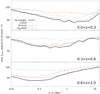 |
Fig. 7. Percentage fraction in total marginal posterior error of fδ, mn due to uncertainties in the lensing kernel and IA parameter. Shown is the statistical error relative to the full marginal error (RMS variance of posterior) as a function of k in three redshift bins without marginalisation (solid lines), with marginalisation over errors in the source redshift distributions only (dashed lines), Ωm in the lensing kernel only (dash-dotted lines), and for the AIA error only (dotted lines). |
6. Discussion
In this study we presented, verified, and applied to KiDS-1000 data a revised method for reconstructing the three-dimensional (band) matter power spectrum with tomographic shear data. Our approach relies on the specification of a projection kernel only, and is hence agnostic about an analytical model for Pδ(k, z), while being applicable for all cosmologies where the ξ±(ij)(θ) are projections of Pδ(k, z) along the line of sight. Numerically convenient, we express Pδ(k, z) = : fδ(k, z) Pδfid(k, z) in terms of a reference and probe deviations, fδ, mn ∈ [0, 100], relative to it, putting the free variables fδ, mn into the same dynamical range. Not required, however, is a reference close to the true power spectrum; for instance, in Fig. 2 we use a reference fixed in cosmic time to highlight the structure growth, or, on the extreme end, a constant Pδfid(k, z)≡P0 would yield a fδ, mn that directly represents the power spectrum. The rescaling of Pδfid(k, z) by a constant inside any z-bin, whilst redefining fδ, mn, does not affect the inferred Δ2(k, z)∝fδ(k, z) Pδfid(k, z); the reconstructed matter power spectrum is robust against the reference used. Choosing a reference towards a slowly evolving fδ(k, z) is nevertheless preferable because the z-bin-average that the fδ, mn represent depends on the specific noise properties and source z-distributions in the tomographic survey; a comparison to theoretical models will have to replicate the data-specific z-weighting more closely for a significantly varying fδ(k, z) inside a wide z-bin. This is obvious in Fig. 2 for a z-independent reference, where more weight is given closer to the lower boundary of each z-bin: the average fδ, mn is close to the true fδ(k, z) near zmax = 0.13, 0.4, 0.7 for Z1, Z2, and Z3; yet the bin centres are at zmid = 0.15, 0.45, 1.30. Although a best-fitting ΛCDM model without baryonic feedback or neutrinos as reference is a good fit to the data already, as shown by the red lines relative to the black data points in Fig. B.1, the fδ, mn values indicate where additional changes might be needed or how much deviation from the reference is acceptable until we conflict with the data. We proceed here with two variants of the analysis, one for an fδ, mn-average over the full redshift range and one to probe the z-evolution of fδ(k, z).
Our first variant in the left panel of Fig. 4 averages fδ(k, z), denoted  hereafter, over the entire z-range covered by KiDS-1000, with the most signal from essentially z ≲ 1. This analysis shows that in the non-linear regime, k ≈ 0.05–10 h Mpc−1, the KiDS-1000 matter power-spectrum is consistent with the ΛCDM reference in Table 1 within 20% (68% CI). Therefore, there is no evidence for a variation, suppression or boost, exceeding 20% relative to the reference scenario with cold dark matter (excluding neutrino suppression and baryon feedback). This is also within the range reported by other lensing studies, discussed below, although we caution that the results are not always one-to-one comparable to ours because they are partly based on the premise that the lensing Pδ(k, z) has the PlanckS8 (Planck Collaboration VI 2020), but is attenuated in the non-linear regime to fit the lensing measurements of significantly lower S8 to explain the so-called S8 tension. Such an attenuation, if present, would be addressed in our reference by a systematically lower S8 instead of fully showing up in
  , especially because our data lack constraining power in the unattenuated linear regime, k ≲ 0.01 h Mpc−1. To level the field with analyses using the PlanckS8 as the premise, we changed the reference to a power spectrum with Planck cosmology, ΔPlanck2(k, z), and recast Fig. 4, left panel, into Fig. 8 for the ratio
  at
at  , a redshift where the lensing method is roughly the most sensitive. Only from this Planck perspective do our results now clearly require a suppression, 1 − fδ, mn, of the ΛCDM reference at k ≈ 3 h Mpc−1 of up to 35%±15%±25% (68% and 95% CI). As indicated by the lines in the plot, it is conceivable to explain the tension with Planck by a variety of hypothetical mechanisms involving, among other things, extreme baryonic feedback, (sterile) neutrinos, or alternatives to non-interacting cold dark matter.
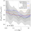 |
Fig. 8. Power spectrum ratio ΔKiDS2(k, z)/ΔPlanck2(k, z) at z = 0.5. Shown in grey are the 68% and 95% CI from our analysis. The KiDS-1000 spectrum ΔKiDS2(k, z) uses the fδ, mn in Fig. 4 averaged within one broad redshift bin (left panel). The Planck model for ΔPlanck2(k, z) is the TT, TE, EE+lowE best fit of a standard ΛCDM (Planck Collaboration VI 2020) extrapolated to z = 0.5 with HMCode2020 by Mead et al. (2021). The lines are model transfer functions to ΔPlanck2(k, z) invoking flavours of extreme baryonic feedback (HMCode2020: log10(TAGN/K) = 8.8, Abaryon = 3.13, ηbaryon = 0.603; BCM by Schneider & Teyssier 2015: log10(Mc/h−1 M⊙) = 15.0792, ηb = 0.5, ks = 55.0), neutrino suppression for cumulative neutrino masses ∑νmν (BCM), or a mixture of CDM and WDM (Kamada et al. 2016, mwdm: WDM particle mass, fwdm: WDM mass fraction). |
Therefore, whereas a CDM power spectrum without suppression and low S8 is on average a good description of the KiDS-1000 shear tomography, small modifications to CDM would be insufficient to reconcile KiDS-1000 with Planck: mechanisms with a substantial suppression (more than 20%) have to be invoked, in agreement with other recent studies analysing KiDS-1000 lensing data. For instance, the recent Schneider et al. (2022, S+22) combines KiDS-1000 data with observations of X-ray emission and the kinematic Sunyaev–Zeldovich (kSZ) effect in galaxy clusters to inform baryonic feedback parameters incorporated in their ΛCDM-flavoured Pδ(k, z). By initially using the KiDS-1000 data alone, the deviations from their model without baryonic feedback are inconclusive but remain, as in our measurement in the left panel of Fig. 4, within 10–20% for k = 1–10 h Mpc−1 (68% CI). Only when adding the X-ray and kSZ data do their constraints strongly favour a power suppression of up to 30% (68% CI) at k ≈ 5 h Mpc−1, somewhat more than our data support. Building only on lensing information, Preston et al. (2023, PEG23) analyse KiDS-1000 and data from the third-year Dark Energy Survey (DES Y3) to extend a ΛCDM model by one modification parameter, Amod, pushing the non-linear Pδ(k, z), equivalent to Amod = 1, towards the linear power spectrum, Amod = 0. Their KiDS-1000 fit with uninformative priors on cosmological parameters and Amod ∈ [ − 5, 5] is, as in Fig. 4, inconclusive, Amod ≈ 0.9 ± 0.2 (their Figure 2, left panel). However, when assuming a Planck cosmology and the suppression-inclined prior Amod ∈ [0.5, 1], PEG23 claim strong evidence for a suppression of ≈25%±6% at k ≈ 3 h Mpc−1 (68% CI), more significant yet fully consistent with our Fig. 8 (we reiterate our relaxed prior fδ, mn ∈ [0, 102]). Furthermore, Broxterman & Kuijken (2024, BK24) fit a double power law Pδ(k, z)∝kp (1 + z)−mBK to ξ±(ij)(θ) for KiDS-1000, DES Y3, and the third year Hyper Suprime-Cam Survey (HSC Y3), yielding a reasonable ΛCDM match without suppression in the range k = 0.01–5 h Mpc−1 (68% CI) and a 2σ agreement among the three Stage III surveys. Compared to our results for Nz = 1, similarly averaging over the full redshift range, their constraints are weaker in the non-linear regime ( ), despite the same data, probably because of our tighter Ωm prior for the projection kernel: the Pδ(k, z) amplitude in ξ±(ij)(θ) is degenerate with the pre-factor Ωm2 in the Eqs. (8)–(10). Finally, similar results are reported by authors that use only DES Y3 lensing data although the required suppression in the non-linear regime relative to Planck tends to be somewhat lower than for KiDS-1000 by a factor between one and two (Bigwood et al. 2024, PEG23, Ferreira et al. 2024, Aricò et al. 2023). Utilising lensing probes alone, Perez Sarmiento et al. (2025) demonstrates consistency with the Planck cosmology on linear scales, yet reveals a 20–25% suppression in the non-linear regime, by combining DES Y3 and CMB lensing data. In conclusion, other works support our finding of an average matter power-spectrum that at k ≳ 0.05 h Mpc−1 is either, within 20% tolerance, a purely ΛCDM spectrum of low S8 ≈ 0.73, or a spectrum with both higher PlanckS8 ≈ 0.83 and significant suppression of up to 20%–30% in the non-linear regime relative to CDM.
Surprisingly, our KiDS-1000 analysis becomes more complex and discrepant with our best-fitting ΛCDM reference of low S8 if the fδ, mn, unlike in previous studies, are free to vary with redshift, achieved in our second analysis by increasing the number of z-bins to Nz = 3 broad z-bins. This is only practical by employing Tikhonov regularisation, or something else to this effect, as clearly illustrated by the dramatically shrinking sizes of the credible regions from τ = 0 to τ = 5 in Fig. 2. Applied to KiDS-1000, the 68% CI constraints in the middle panel of Fig. 4 then depict a remarkably diverse picture: only the fδ, mn in the low-z bin, Z1 = [0, 0.3], are now consistent with the reference matter power spectrum, averaged for all k-bins to 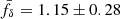 , whereas the power spectrum in Z2 = [0.3, 0.6] is overall suppressed,
 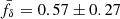 , and boosted for Z3 = [0.6, 2], where
  . The verification tests in Appendix A, for analytic data (noisy) vectors, and in Sect. 5.5, for mock N-body shear catalogues, assure us of an fδ, mn accuracy of 10% or better within k ≈ 0.01–10 h Mpc−1. The observed tendency of shifting the median posterior fδ, mn of our 68% CIs towards
  for Z3 and towards
  –0.9 for Z2, due to the broadened skewed posterior PDFs in these z-bins, actually goes in the direction of the KiDS-1000 result. It is nevertheless too small for the pronounced split between Z2 and Z3 credible regions in the real data, which also are, unlike the verification results, blurred by the IA and lensing kernel uncertainties (an extra ∼10% error, Fig. 7). For the baseline fδ(k, z)≡1 in Fig. A.5, the split in the mock data realisations is not nearly as pronounced as for KiDS-1000, making the KiDS-1000 result very roughly a 1/16 ≈ 6% event, or less, for the baseline scenario.
To explore the possibility of spurious systematic errors possibly mimicking the evolving fδ(k, z), we estimated in three scenarios the amplitude of bias needed to replicate our KiDS-1000 results if the ΛCDM reference were the true matter power spectrum. First, a spurious shear m-bias in the data is assumed to be the dominating source of systematic error. The required bias is then obtained through fitting  , predicted by the reference model, to the KiDS-1000 data vector by maximising the data likelihood, Eq. (25), with respect to the bias parameters mi in the tomographic bins i. The corresponding (posterior median) fδ, mn of the best-fitting model are plotted as data points with filled squares in Fig. 9 in comparison to KiDS-1000 (shaded regions). Evidently, the m-bias model closely traces the KiDS-1000 results, but, according to its best-fit parameters {mi}={+1.00, +0.48, −0.023, −0.028, +0.035}, it needs an unrealistic m-bias in the first two source bins that exceeds the reported values in Asgari et al. (2021) by more than 30σ. The second scenario assumes spurious photo-z errors in pz(i)(z) as dominating source of bias. Again, we fit a
  to the KiDS-1000 data vector, now for the pz(i)(z + δzi) shifted by the bias parameters δzi, while the reconstruction uses the original pz(i)(z). The best-fit values are {δzi}={−0.075, −0.079, +0.009, +0.018, −0.052}. As in the previous m-bias scenario, this model fits the KiDS-1000 results equally well (filled circles in Fig. 9), but requires a high bias (photo-zs are systematically low) in the first two and the last source z-bins. This bias level exceeds the estimated tolerances of photo-z errors in the KiDS-1000 gold sample by more than 5σ (Table 2). A third conceivable source of systematic error is an IA model bias. Too simplistic physically, the approximations in the NLA model are nevertheless flexible enough to fit measurements of IA as a means for calibrating the IA distortion of ξ±(ij)(θ) (Fortuna et al. 2021; Preston et al. 2024). It may be, however, that z-binning of Δ2(k, z) makes us sensitive to a z-dependent IA amplitude, missing in the NLA model and typically irrelevant in Stage III cosmological analyses. To test if a z-dependent IA amplitude AIA(z):=AIA′ (1 + z)η (1 + zpiv)−η, as in the eNLA model, potentially explains the fδ, mn data after all, we fit
  to KiDS-1000 by varying {AIA′,zpiv, η} only, yielding the parameters {0.3, 0.19, 1.5} for the open diamond data points in Fig. 9. Crucially, the reconstruction algorithm is ignorant about AIA(z) and assumes a constant AIA. Indeed, then some of the split between Z2 and Z3 (especially the drop in Z2) could be explained by the IA model bias. And, since zpiv = 0.3 and η = 1.5 are deemed consistent with KiDS-1000 uncertainties in Asgari et al. (2021), this hypothesis is a plausible explanation for at least part of the
  redshift variation. More plausible still is a combination of AIA(z) and a moderate photo-z bias, 2σ–4σ, indicated by the crosses in Fig. 9. Lastly, recalling the 1σ–2σ evidence for B-modes in Sect. 4.3, a systematic shear error might also be relevant here. However, we lack a KiDS-1000 model of these for ξ±(ij), and it is unclear if they plausibly contribute to the
  result. In summary, whereas (especially) m-biases and photo-z biases alone are unlikely sources of systematic errors that shape the result of evolving
  , the negligence of a z-dependent IA amplitude, AIA, as in our reconstruction set-up, in combination with moderate photo-z biases might explain our Nz = 3 result. At this point, we are unable to exclude either possibility, or that of small systematic errors related to B-modes, but note that the discussed scenarios mainly target the first two tomographic bins, zB ≤ 0.5, where the posterior predictive of the model also indicates some conflict with the data (Fig. B.1). Future reconstructions of the matter power spectrum inside separate redshift bins should also pay close attention to the IA modelling.
 |
Fig. 9. KiDS-1000 results for fδ, mn, as in the middle panel of Fig. 4, in relation to alternative hypotheses using the reference cosmology Pδfid(k, z) and best-fitting bias parameters to match the KiDS-1000 data vector, ξ±(ij)(θ). The filled squares assume shear m-bias factors {mi}={+1.00, +0.48, −0.023, −0.028, +0.035}, the filled circles assume photo-z biases {δzi}={−0.075, −0.079, +0.009, +0.018, −0.052}, and the open diamonds employ the eNLA model with {AIA′,zpiv, η}={0.3, 0.19, 1.5}. The crosses assume a hybrid model of eNLA and a smaller z-bias: {AIA′,zpiv, η}={0.45, 0.25, 2.3} and {δzi}={−0.017, −0.058, +0.027, +0.025, −0.043}. The data points indicate the posterior median (CIs are similar to those of the shaded regions); the filled data points use alternating k-bins to avoid overlap. |
A truly evolving fδ(k, z), on the other hand, would offer insights into the physics of non-linear structure growth at k ≳ 0.1 h Mpc−1 and z ≲ 1. In brief, the KiDS-1000 data indicate too little power for the epoch z ≈ 0.3–0.6 and too much power for z ≈ 0.6–2, compared to the purely-ΛCDM reference model that actually matches the fδ, mn averaged in a single z-bin (68% CI). Phrasing this a bit more carefully, this statement applies to weighted averages inside three wide z-bins where most weight is given to Δ2(k, z) around z ≈ 0.13, 0.4, 0.7 for Z1, Z2, and Z3, similar to Fig. 2. Even so, the average deviations in the Z2 and Z3 are, in fact, such that they make Δ2(k, z) inside the bins statistically consistent (right panel of Fig. 4), independent of the chosen reference – thus there is no significant detection of any growth from about z = 0.7 to 0.4. The only increase in power is detected towards lower z ≈ 0.13. This qualitatively matches the S8-tension: cosmological probes that give more weight to z ≳ 0.7, such as CMB experiments, would observe a Δ2(k, z) with amplitude higher than in our reference, hence a higher S8, whereas probes more sensitive to z ∼ 0.4 or lower, such as lensing experiments, would observe a Δ2(k, z) with S8 equal to our reference or even lower. We are not aware of a similar conclusion in the lensing literature, although the recent BK24 report a vanishing growth rate at 1σ, their growth index mBK, for KiDS-1000 and HSC Y3 (yet not for DES Y3). That finding for mBK might be related to our result, depending on how the Z1–Z3 are effectively weighted in the BK24 analysis. Possible physical causes of the peculiar structure growth in KiDS-1000 compared to the reference model are, however, presumably non-trivial and beyond the scope of this paper. For example, a baryonic feedback model would have to be strongly evolving with redshift below z ∼ 1 (and non-monotonic) to match the KiDS-1000 fδ, mn, typically not found in state-of-the art models (e.g., Schaller et al. 2025, and references therein).
Finally, the close connection of the S8-tension to the KiDS-1000 result for Δ2(k, z) in Nz = 3 z-bins makes this an interesting case, either as evidence in favour of modifications towards the structure growth in the ΛCDM reference, or in favour of spurious systematic errors in a shear tomography analysis mimicking the tension. This evidence appears to be unnoticed in previous Stage III analyses – a full analytic model of Δ2(k, z) fitted to the shear tomography can give an unsuspecting match similar to our Nz = 1 analysis – so that a confirmation of the KiDS-1000 result with other lensing data is important. Furthermore, looking forward not too far into the future, Stage IV data will be available soon with roughly 20 times the survey area of KiDS-1000 and also deeper observations, with surveys such as the space-based missions Euclid and Roman, or the ground-based survey by Rubin. Of these the Euclid Wide Survey will provide tomographic measurements within 13 source z-bins up to z ∼ 2.5, statistical errors reduced by about one order of magnitude compared to Stage III, and an excellent control of systematic errors for shear and photo-z. We see no restriction to applying our reconstruction technique to Stage IV data, merely assuming a lensing kernel and an IA model (possibly updated and carefully calibrated). This promises measurements of the matter power spectrum at different redshifts to unprecedented precision, perhaps up to z ∼ 2 with Nz = 4 or more bins, critically testing models of the non-linear structure growth.
The KiDS data products are public and available through http://kids.strw.leidenuniv.nl/DR4
Sample variance of the large-scale structure introduces a correlation between the scatter of δzi across different tomographic redshift bins, see Figure 2 in Hildebrandt et al. (2021) for the explicit values.
Acknowledgments
This paper went through the KiDS review process. We also want to thank Jeger Broxtermann for useful comments. LP acknowledges support from the DLR grant 50QE2002. PB acknowledges financial support from the Canadian Space Agency (Grant No. 23EXPROSS1) and the Waterloo Centre for Astrophysics. Some results in this paper are based on observations made with ESO Telescopes at the La Silla Paranal Observatory under programme IDs 177.A-3016, 177.A- 3017, 177.A-3018 and 179.A-2004, and on data products produced by the KiDS consortium. The KiDS production team acknowledges support from: Deutsche Forschungsgemeinschaft, ERC, NOVA and NWO-M grants; Target; the University of Padova, and the University Federico II (Naples).
References
- Abbott, T. M. C., Abdalla, F. B., Alarcon, A., et al. 2018, Phys. Rev. D, 98, 043526 [NASA ADS] [CrossRef] [Google Scholar]
- Alam, S., Albareti, F. D., Allende Prieto, C., et al. 2015, ApJS, 219, 12 [Google Scholar]
- Aricò, G., Angulo, R. E., Zennaro, M., et al. 2023, A&A, 678, A109 [NASA ADS] [CrossRef] [EDP Sciences] [Google Scholar]
- Asgari, M., Lin, C.-A., Joachimi, B., et al. 2021, A&A, 645, A104 [NASA ADS] [CrossRef] [EDP Sciences] [Google Scholar]
- Bacon, D. J., Taylor, A. N., Brown, M. L., et al. 2005, MNRAS, 363, 723 [Google Scholar]
- Bartelmann, M., & Schneider, P. 2001, Phys. Rep., 340, 291 [Google Scholar]
- Begeman, K., Belikov, A. N., Boxhoorn, D. R., & Valentijn, E. A. 2013, Exp. Astron., 35, 1 [NASA ADS] [Google Scholar]
- Benítez, N. 2000, ApJ, 536, 571 [Google Scholar]
- Bigwood, L., Amon, A., Schneider, A., et al. 2024, MNRAS, 534, 655 [NASA ADS] [CrossRef] [Google Scholar]
- Blake, C., Amon, A., Childress, M., et al. 2016, MNRAS, 462, 4240 [NASA ADS] [CrossRef] [Google Scholar]
- Bridle, S., & King, L. 2007, New J. Phys., 9, 444 [Google Scholar]
- Brooks, S., Gelman, A., Jones, G., & Meng, X. 2011, Handbook of Markov Chain Monte Carlo, Chapman& Hall/CRC Handbooks of Modern Statistical Methods (CRC Press) [CrossRef] [Google Scholar]
- Broxterman, J. C., & Kuijken, K. 2024, A&A, 692, A201 [NASA ADS] [CrossRef] [EDP Sciences] [Google Scholar]
- Bucko, J., Giri, S. K., Peters, F. H., & Schneider, A. 2024, A&A, 683, A152 [NASA ADS] [CrossRef] [EDP Sciences] [Google Scholar]
- Burger, P. A., Porth, L., Heydenreich, S., et al. 2024, A&A, 683, A103 [NASA ADS] [CrossRef] [EDP Sciences] [Google Scholar]
- Crittenden, R. G., Natarajan, P., Pen, U.-L., & Theuns, T. 2001, ApJ, 559, 552 [CrossRef] [Google Scholar]
- Croft, R. A. C., & Metzler, C. A. 2000, ApJ, 545, 561 [NASA ADS] [CrossRef] [Google Scholar]
- Edge, A., Sutherland, W., Kuijken, K., et al. 2013, The Messenger, 154, 32 [NASA ADS] [Google Scholar]
- Erben, T., Schirmer, M., Dietrich, J. P., et al. 2005, Astron. Nachr., 326, 432 [NASA ADS] [CrossRef] [Google Scholar]
- Euclid Collaboration (Mellier, Y., et al.) 2025, A&A, 697, A1 [Google Scholar]
- Fenech Conti, I., Herbonnet, R., Hoekstra, H., et al. 2017, MNRAS, 467, 1627 [NASA ADS] [Google Scholar]
- Ferreira, T., Alonso, D., Garcia-Garcia, C., & Chisari, N. E. 2024, Phys. Rev. Lett., 133, 051001 [Google Scholar]
- Fortuna, M. C., Hoekstra, H., Joachimi, B., et al. 2021, MNRAS, 501, 2983 [NASA ADS] [CrossRef] [Google Scholar]
- García-García, C., Zennaro, M., Aricò, G., Alonso, D., & Angulo, R. E. 2024, JCAP, 2024, 024 [CrossRef] [Google Scholar]
- Gelman, A., & Rubin, D. B. 1992, Stat. Sci., 7, 457 [Google Scholar]
- Gelman, A., Carlin, J., Stern, H., & Rubin, D. 2003, Bayesian Data Analysis, Chapman& Hall/CRC Texts in Statistical Science (Chapman& Hall/CRC) [Google Scholar]
- Giblin, B., Heymans, C., Asgari, M., et al. 2021, A&A, 645, A105 [NASA ADS] [CrossRef] [EDP Sciences] [Google Scholar]
- Harnois-Déraps, J., van Waerbeke, L., Viola, M., & Heymans, C. 2015, MNRAS, 450, 1212 [Google Scholar]
- Harnois-Déraps, J., Martinet, N., & Reischke, R. 2022, MNRAS, 509, 3868 [Google Scholar]
- Hartlap, J., Simon, P., & Schneider, P. 2007, A&A, 464, 399 [NASA ADS] [CrossRef] [EDP Sciences] [Google Scholar]
- Heymans, C., Grocutt, E., Heavens, A., et al. 2013, MNRAS, 432, 2433 [Google Scholar]
- Heymans, C., Tröster, T., Asgari, M., et al. 2021, A&A, 646, A140 [NASA ADS] [CrossRef] [EDP Sciences] [Google Scholar]
- Hilbert, S., Hartlap, J., White, S. D. M., & Schneider, P. 2009, A&A, 499, 31 [NASA ADS] [CrossRef] [EDP Sciences] [Google Scholar]
- Hildebrandt, H., van den Busch, J. L., Wright, A. H., et al. 2021, A&A, 647, A124 [EDP Sciences] [Google Scholar]
- Hinshaw, G., Larson, D., Komatsu, E., et al. 2013, ApJS, 208, 19 [Google Scholar]
- Hirata, C. M., & Seljak, U. 2004, Phys. Rev. D, 70, 063526 [Google Scholar]
- Hu, W., & Keeton, C. R. 2002, Phys. Rev. D, 66, 063506 [Google Scholar]
- Jarvis, M. 2015, Astrophysics Source Code Library [record ascl:1508.007] [Google Scholar]
- Jarvis, M., Bernstein, G., & Jain, B. 2004, MNRAS, 352, 338 [Google Scholar]
- Jing, Y. P., Zhang, P., Lin, W. P., Gao, L., & Springel, V. 2006, ApJ, 640, L119 [Google Scholar]
- Joachimi, B., & Schneider, P. 2008, A&A, 488, 829 [NASA ADS] [CrossRef] [EDP Sciences] [Google Scholar]
- Joachimi, B., Mandelbaum, R., Abdalla, F. B., & Bridle, S. L. 2011, A&A, 527, A26 [NASA ADS] [CrossRef] [EDP Sciences] [Google Scholar]
- Joachimi, B., Lin, C. A., Asgari, M., et al. 2021, A&A, 646, A129 [NASA ADS] [CrossRef] [EDP Sciences] [Google Scholar]
- Kaiser, N. 1992, ApJ, 388, 272 [Google Scholar]
- Kamada, A., Inoue, K. T., & Takahashi, T. 2016, Phys. Rev. D, 94, 023522 [Google Scholar]
- Kilbinger, M. 2015, Rep. Prog. Phys., 78, 086901 [Google Scholar]
- Kilbinger, M., Heymans, C., Asgari, M., et al. 2017, MNRAS, 472, 2126 [Google Scholar]
- Kuijken, K. 2011, The Messenger, 146, 8 [NASA ADS] [Google Scholar]
- Kuijken, K., Heymans, C., Hildebrandt, H., et al. 2015, MNRAS, 454, 3500 [Google Scholar]
- Kuijken, K., Heymans, C., Dvornik, A., et al. 2019, A&A, 625, A2 [NASA ADS] [CrossRef] [EDP Sciences] [Google Scholar]
- Laguë, A., Schwabe, B., Hložek, R., Marsh, D. J. E., & Rogers, K. K. 2024, Phys. Rev. D, 109, 043507 [Google Scholar]
- Lamman, C., Tsaprazi, E., Shi, J., et al. 2024, Open J. Astrophys., 7, 14 [NASA ADS] [CrossRef] [Google Scholar]
- Li, X., Zhang, T., Sugiyama, S., et al. 2023, Phys. Rev. D, 108, 123518 [CrossRef] [Google Scholar]
- Mauland, R., Winther, H. A., & Ruan, C.-Z. 2024, A&A, 685, A156 [NASA ADS] [CrossRef] [EDP Sciences] [Google Scholar]
- Mead, A. J., Peacock, J. A., Heymans, C., Joudaki, S., & Heavens, A. F. 2015, MNRAS, 454, 1958 [NASA ADS] [CrossRef] [Google Scholar]
- Mead, A. J., Brieden, S., Tröster, T., & Heymans, C. 2021, MNRAS, 502, 1401 [Google Scholar]
- Mezzetti, M., Bonometto, S. A., Casarini, L., & Murante, G. 2012, JCAP, 2012, 005 [Google Scholar]
- Miller, L., Heymans, C., Kitching, T. D., et al. 2013, MNRAS, 429, 2858 [Google Scholar]
- Murata, K., & Takeuchi, T. T. 2022, PASJ, 74, 1329 [Google Scholar]
- Pen, U.-L., Lu, T., van Waerbeke, L., & Mellier, Y. 2003, MNRAS, 346, 994 [Google Scholar]
- Perez Sarmiento, K., Laguë, A., Madhavacheril, M., Jain, B., & Sherwin, B. 2025, ArXiv e-prints [arXiv:2502.06687] [Google Scholar]
- Planck Collaboration VI. 2020, A&A, 641, A6 [NASA ADS] [CrossRef] [EDP Sciences] [Google Scholar]
- Pranjal, R., Krause, E., Dolag, K., et al. 2025, JCAP, 2025, 041 [Google Scholar]
- Preston, C., Amon, A., & Efstathiou, G. 2023, MNRAS, 525, 5554 [NASA ADS] [CrossRef] [Google Scholar]
- Preston, C., Amon, A., & Efstathiou, G. 2024, MNRAS, 533, 621 [NASA ADS] [CrossRef] [Google Scholar]
- Salcido, J., McCarthy, I. G., Kwan, J., Upadhye, A., & Font, A. S. 2023, MNRAS, 523, 2247 [NASA ADS] [CrossRef] [Google Scholar]
- Schaller, M., Schaye, J., Kugel, R., Broxterman, J. C., & van Daalen, M. P. 2025, MNRAS, submitted [arXiv:2410.17109] [Google Scholar]
- Schneider, P. 2006, in Saas-Fee Advanced Course 33: Gravitational Lensing: Strong, Weak and Micro, eds. G. Meylan, P. Jetzer, & P. North, 269 [Google Scholar]
- Schneider, A., & Teyssier, R. 2015, JCAP, 2015, 049 [Google Scholar]
- Schneider, P., van Waerbeke, L., Kilbinger, M., & Mellier, Y. 2002, A&A, 396, 1 [NASA ADS] [CrossRef] [EDP Sciences] [Google Scholar]
- Schneider, P., Eifler, T., & Krause, E. 2010, A&A, 520, A116 [NASA ADS] [CrossRef] [EDP Sciences] [Google Scholar]
- Schneider, A., Giri, S. K., Amodeo, S., & Refregier, A. 2022, MNRAS, 514, 3802 [NASA ADS] [CrossRef] [Google Scholar]
- Secco, L. F., Samuroff, S., Krause, E., et al. 2022, Phys. Rev. D, 105, 023515 [NASA ADS] [CrossRef] [Google Scholar]
- Seljak, U. 1998, ApJ, 506, 64 [Google Scholar]
- Simon, P. 2012, A&A, 543, A2 [NASA ADS] [CrossRef] [EDP Sciences] [Google Scholar]
- Simon, P., & Hilbert, S. 2018, A&A, 613, A15 [NASA ADS] [CrossRef] [EDP Sciences] [Google Scholar]
- Smith, R. E., & Markovic, K. 2011, Phys. Rev. D, 84, 063507 [Google Scholar]
- Smith, R. E., Peacock, J. A., Jenkins, A., et al. 2003, MNRAS, 341, 1311 [Google Scholar]
- Spergel, D., Gehrels, N., Baltay, C., et al. 2015, ArXiv e-prints [arXiv:1503.03757] [Google Scholar]
- Sugiyama, N. 1995, ApJS, 100, 281 [NASA ADS] [CrossRef] [Google Scholar]
- Takahashi, R., Sato, M., Nishimichi, T., Taruya, A., & Oguri, M. 2012, ApJ, 761, 152 [Google Scholar]
- Takahashi, R., Hamana, T., Shirasaki, M., et al. 2017, ApJ, 850, 24 [Google Scholar]
- Tegmark, M., & Zaldarriaga, M. 2002, Phys. Rev. D, 66, 103508 [NASA ADS] [CrossRef] [Google Scholar]
- The LSST Dark Energy Science Collaboration (Mandelbaum, R., et al.) 2018, ArXiv e-prints [arXiv:1809.01669] [Google Scholar]
- Tröster, T., Asgari, M., Blake, C., et al. 2021, A&A, 649, A88 [NASA ADS] [CrossRef] [EDP Sciences] [Google Scholar]
- Truttero, O., Zuntz, J., Pourtsidou, A., & Robertson, N. 2025, Open J. Astrophys., 8, 19 [Google Scholar]
- Wright, A. H., Hildebrandt, H., van den Busch, J. L., & Heymans, C. 2020a, A&A, 637, A100 [NASA ADS] [CrossRef] [EDP Sciences] [Google Scholar]
- Wright, A. H., Hildebrandt, H., van den Busch, J. L., et al. 2020b, A&A, 640, L14 [NASA ADS] [CrossRef] [EDP Sciences] [Google Scholar]
- Ye, G., Jiang, J. Q., & Silvestri, A. 2024, ArXiv e-prints [arXiv:2411.07082] [Google Scholar]
- Yoshida, H. 1990, Phys. Lett. A, 150, 262 [NASA ADS] [CrossRef] [Google Scholar]
Appendix A: Hamiltonian Monte Carlo algorithm and code verification
The Bayesian reconstruction of the 3D matter power spectrum, expressed by π = (…,fδ, mn, …), is numerically challenging due to the high number of variables, up to Nz × Nk = 60 or more in future Stage IV applications. As practical solution, the following describes our implementation details of a Hamiltonian Monte Carlo sampler of the posterior PDF P(π|d), as well as our verification and convergence tests. Compared to a Metropolis-Hastings algorithm, this MCMC approach has an improved convergence and quicker decorrelation – but requires first-order derivatives of the posterior PDF. The derivatives were here easily obtained analytically, contrary to previous KiDS-1000 cosmology analyses where other MCMC algorithms are used. We focus on the specifics of our implementation but refer to Brooks et al. (2011) for more background information.
A.1. Basic concept
In brief, the Hamiltonian MCMC algorithm is based on the insight from statistical mechanics that a canonical ensemble of particles j = 1…Nz × Nk with generalised coordinates πj, masses mj, canonical moments pj, the Hamiltonian
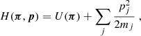 (A.1)
(A.1)
and temperature parameter β randomly occupies states in phase space according to the PDF
![Mathematical equation: $$ \begin{aligned}&f(\boldsymbol{\pi },\boldsymbol{p}) = \frac{1}{Z}\exp {\Big (-\beta \,H[\boldsymbol{\pi },\boldsymbol{p}]\Big )}\nonumber \\&\quad =\frac{1}{Z}\, \exp {\Big (-\beta \,U[\boldsymbol{\pi }]\Big )} \,\exp {\left(-\beta \,\sum _j\frac{p_j^2}{2m_j}\right)}\;, \end{aligned} $$](/articles/aa/full_html/2025/06/aa54017-25/aa54017-25-eq107.gif) (A.2)
(A.2)
where the partition function, Z, is a normalisation constant. Turning this insight around, our sampler simulates a canonical ensemble following individual particles along trajectories under the influence of the potential U(π) = − lnP(π|d) to trace the posterior PDF, P(π|d). The trajectory of each particle is determined by the symplectic Hamilton equations
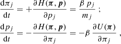 (A.3)
(A.3)
interrupted by random jumps between hyper-planes of constant energy,  , such that energy levels change from E to E′ with probability min{1, eβ(E − E′)}. These random events simulate the transfer of energy between particles and a heat bath of temperature T ∝ β−1. Ignoring the moments pj, the distribution of states πi of an ensemble of particles then samples the marginalised PDF
![Mathematical equation: $$ \begin{aligned} \int _{V_{\boldsymbol{p}}}\mathrm{d}\boldsymbol{p}\;f(\boldsymbol{\pi },\boldsymbol{p})\propto \exp {\Big (-\beta \,U[\boldsymbol{\pi }]\Big )}= \left[P(\boldsymbol{\pi }|\boldsymbol{d})\right]^\beta \;. \end{aligned} $$](/articles/aa/full_html/2025/06/aa54017-25/aa54017-25-eq110.gif) (A.4)
(A.4)
This does not mean, however, moments can be chosen arbitrarily. Instead, the pj obey the Gaussian distribution of a maximum-entropy ensemble in f(π, p) and, therefore, are randomly set to  , where σp2 = mj/β, in the algorithm below. For convenience, we set the heat bath temperature to β ≡ 1, thus the ensemble πi samples the posterior P(π|d), as needed.
A.2. Implementation details
The art of optimising the Hamiltonian MCMC is in the way we evolve states in the canonical ensemble, how we switch between energy levels, which sampling points are kept, and how particle masses, mj, are chosen. For our application, we found sufficient convergence already when using a simplistic model of equal mass weights, mj ≡ 1. Furthermore, to produce a sequence of sampling points πi, we followed the MCMC standard procedure.
-
We pick a random starting point, π, i = 0.
-
The elements of the momentum in p, conjugate to π, are randomised independently,
 .
. -
The algorithm then numerically integrates the Hamilton Eqs. (A.3) with a symplectic integrator to follow the trajectory, starting from (π, p), for n equal time steps Δt, proposing the end point as a new MCMC point, (πnΔt, pnΔt).
-
This proposal πnΔt is accepted with probability min{1, eβ(E − EnΔt)}, where E := H(π, p) and EnΔt := H(πnΔt, pnΔt) are the energies of the initial and the proposed new state. If rejected, we go back to the initial trajectory point, π, and start again from step 2.
-
If accepted, we keep the proposed state as MCMC data point, πi = πnΔt. Since rejections mean we have to go back and reuse a sampling point, the stored πi has weight wi = 1 + nr, i, where nr, i denotes the number of rejections needed for πi.
-
We stop after nmcmc accepted sampling points (πi, wi), or start over again from step 2 with π = πi and i → i + 1 otherwise.
In contrast to Metropolis-Hastings, the Hamiltonian method proposes a new MCMC point by (approximately) transporting the previous point along the iso-contours of the posterior density, keeping the rejection rate low even if the previous and proposed point are well separated, thereby decorrelating sampling points. Notably, this way of proposing new points is symmetric due to the time symmetry of the Hamilton equations and the isotropy of the randomised momenta, satisfying the conditions of a detailed balance. In addition, as long as the time symmetry is preserved, unavoidable inaccuracies when numerically integrating Eqs. (A.3) do not bias the sampling, although they usually increase rejection rates when moving too far away from the posterior density iso-contours. As discussed in Brooks et al. (2011), the leapfrog method is a suitable choice as numerical integrator of (A.3) for a MCMC sampler due to its symplectic symmetry. To increase the acceptance rate for larger time steps Δt, we use the more accurate fourth-order, also symplectic, integrator. The various integrator steps are not spelt out here in detail to save space but can be found in Yoshida (1990).
To control the rejection rate of the MCMC sampler, we adjusted the size of a time step, Δt. Decreasing the time step, Δt, typically lowers the rejection rate, but boosts correlations between the sampling points. Starting from Δt = 10−3, we followed the heuristic to keep the rejection rate somewhere around 30% by (i) decreasing  , if the rate exceeds 50%, or (ii) by increasing Δt → 1.2 Δt, if it falls below 16%, after 20 consecutive accepted sampling points. At the same time, the number of trajectory steps was fixed to n = 100. With these settings, the time steps stabilise typically around Δt = 10−2. As final data product, we kept nmcmc = 5 × 10⁴ sampling points after a burn-in phase of 2 × 10⁴ steps during which the step size was continuously adjusted. For all chains, we started the burn-in with the initial state drawn from a normal distribution centred around fδ, mn = 1,
  .
.
To compute the movement along a trajectory by the Hamilton equations, we employed an analytic expression for the gradient
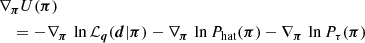 (A.5)
(A.5)
which, for Eq. (24), is split into three summands: one for the likelihood,
 (A.6)
(A.6)
one for the top-hat priors,
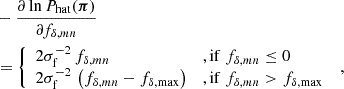 (A.7)
(A.7)
and one for the Tikhonov regularisation,
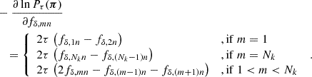 (A.8)
(A.8)
The computation time of the sampler was reduced by computing the matrix  just once and then reusing it for fixed projection parameters q.
A.3. Verification and convergence tests
To validate the convergence of the Monte Carlo sampler, we carried out three different tests using the KiDS-1000 data vector for the projection parameters q as in Table 1. The set-up is identical to that in our analysis in Sect. 5.4 for the most complex model with three redshift bins, Nz = 3. The first test is a sanity check to verify by eye the transition towards a stationary process during the burn-in phase. For this, we inspected as function of iteration i the variation of fδ, mn and the (negative log-) probability −2lnP(π|d) along the chain. The top panel of Fig. A.1 is one random example; other chains and variables fδ, mn in πi look qualitatively similar and are not shown here. Apart from the deep drop of −2lnP at the very beginning of the chain, where the sampler takes the points away from the initial random π, there are no more systematic drifts present for fδ, mn and −2lnP. This indicates a stationary sampling is quickly reached.
The second test, bottom panel of Fig. A.1, quantifies the decorrelation of sampling points, πi, along the chain. For a fair sampling of the posterior density, the sampling points have to become independent quickly. To quantify this, we looked at the correlation coefficients Rmn, kl in the covariance matrix  of two sampling points πi = (…,fδ, mn, …) and πi + δi = (…,fδ, kl, …) separated by a lag of δi iterations along the same chain. The expectation is that the amplitude of Rmn, kl between a pair of model coefficients fδ, mn and fδ, kl decreases towards zero with increasing lag δi. This is indeed the case, as shown in the figure bottom panel for several independent chain runs. The orange curves report for a series of ten MCMCs the trend of the maximum |Rmn, kl| for all coefficient combinations (m, n) and (k, l), the blue curves are the average of all |Rmn, kl|. All chains exhibit the same trend: the maximum |Rmn, kl| quickly falls below a few per cent already after δi ∼ 100, whereas the average |Rmn, kl| is even lower, reaching sub-per cent levels. After that, all curves tend to flat out, probably due to statistical noise in our |Rmn, kl| estimates from the finite number of pairs of sampling points in a given chain.
 |
Fig. A.1. Diagnostic plots of the Hamiltonian MCMC sampler with KiDS-1000 data and our final analysis set-up for fixed projection parameters as in Table 1. Top panel: Example of fδ, mn variations along one random chain at the beginning of the burn-in, starting from the random initial point i = 0 (blue line). The orange line depicts the (negative log-) posterior probability −2lnP(πi|d). Bottom panel: Decrease in the correlation of fδ, mn and fδ, kl with δi iterations lag as estimated in ten randomly chosen, independent chains. The orange lines follows, one line per chain, the maximum absolute-value Pearson correlation coefficient |Rmn, kl|, while the blue lines follows the average |Rmn, kl| over all variable combinations (mn, kl). The sampling points quickly decorrelate after a few hundred iterations; the flattening after lag δi ∼ 100 is due to the statistical error in the estimated |R| for chains of finite length nmcmc = 5 × 10⁴. |
For the third convergence check, we applied the Gelman–Rubin diagnostics to all coefficients fδ, mn individually (Gelman & Rubin 1992). This test probes if a single chain has sufficiently converged, by comparing our nchain = 10 independent MCMC runs. Similar to the marginalisation process, Sect. 3.5, we were not using the full chains but, instead, randomly draw nmerge = 103 points for a thinned each chain. The Gelman–Rubin statistic  is based on the average
  and variance of σδ, mnk2 of fδ, mn within a (thinned) chain k, where W := ∑kσδ, mnk2/nchain is the average of all within-chain variances,
  for
for  is the variance between chains, and
 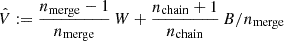 . The ratio B/W follows a F-distribution in the null hypothesis of independent, stationary chains, and normally distributed fδ, mn; and tgr ∼ 1 is to high confidence tgr < 1.1. We repeatedly find tgr < 1.001 for all our free model variables, fδ, mn, consistent with the null hypothesis.
For test reconstructions of the 3D matter power spectrum, Fig. A.2 shows two successful verification runs of the sampler, but now with simulated data, a model correlation vector, d, with added random noise according to the Gaussian likelihood model of the KiDS-1000 data. The verification data assumed a matter power spectrum identical to Pδfid(k, z), thus fδ, mn = 1 for all m and n. In order to not rely on our MCMC code and the X±(ij)(θ; m, n) expansion in particular, we calculated the verification data vector ξ±(ij)(θ), Eq. (7), with a separate computer code from a past study (Simon & Hilbert 2018). The left panel in Fig. A.2, plots the results for fδ, mn averaged over one redshift bin, Nz = 1. The middle panel, uses another noise realisation and splits, as before, fδ, mn into Nz = 3 broad redshift bins to probe the z-evolution. In both panels, we find results consistent with the true values fδ, mn = 1 on a 68% CI level.
 |
Fig. A.2. Reconstructed relative power spectrum, fδ(k, z), in redshift range 0 ≤ z < 2 using a verification data vector mimicking KiDS-1000 data (noise added, not marginalising IA or lensing kernel errors). The true relative power has fδ ≡ 1 for all scales and redshift. The data vector is computed from an independent code, not based on the projection matrix X(ij)(θ; m, n). Shown is the posterior median within a 68% CI. The reconstructions use a Tikhonov parameter of τ = 5.0 and Nk = 20 k-bins. Left panel: The relative power is averaged over the entire redshift range Z1 = [0, 2]. Middle panel: For a relative power that is averaged independently for three redshift bins Z1 = [0, 0.3], Z2 = [0.3, 0.6], and Z3 = [0.6, 2]. Right panel: Dimensionless average power spectrum, Δ2(k, z) = 4π k3Pδfid(k, z) fδ(k, z), interpolated to the centres of the redshift bins Z1 to Z3. |
Increasing the number of z-bins decreases the constraining power for each bin. This adds skewness to the posterior PDF of fδ, mn, especially for Z3, as illustrated by Fig. A.3. The figure shows the posterior PDF of fδ, mn in three z-bins at fixed comoving scale k = 1.8 h Mpc−1 for the NZ = 3 verification data (shaded 68% CI regions). Other scales look qualitatively similar. Notably, the skewness systematically shifts our credible regions towards the long tails in direction of higher fδ values because we report 68% intervals about the median posterior value. This shift for the cyan Z3 regions can also be seen in random realisations of KiDS-1000 mock data, obtained by ray-tracing N-body simulations, in Fig. A.5.
The excellent fit of the model to the verification input data vector, d, is best viewed in the posterior predictive plot, Fig. A.4. This plot compares the posterior model (blue regions for the two CIs 68% and 95% about the median) to the ξ±(ij)(θ) data points with 1σ error bars (black) as function of θ. The lower triangle of panels ‘z–ij’ shows θ ξ−(ij) for the tomographic bin pair (ij), and likewise for the upper triangle and θ ξ+(ij). The data points scatter symmetrically about the median model at the centre of the CIs. Sometimes the residuals exceed 1σ or more, expected statistically for hundreds of (correlated) points. On the whole, we cannot see clear model shortcomings to match the verification data at any angular scale or redshift. This is underscored by the red solid lines for the true (fiducial) ξ±(ij)(θ): the red lines are well within the 68% CI, in dark blue, of the posterior model constraints. Figure B.1 is the same plot but for the actual KiDS-1000 data (Sect. 5.4 provides more details).
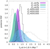 |
Fig. A.3. Posterior PDF of fδ, mn at |
In summary, the foregoing tests demonstrate the excellent convergence of the Hamiltonian Monte Carlo sampler used in the KiDS-1000 analysis and its ability to infer the 3D matter power spectrum with up to Nz × Nk = 60 variables. More tests with fδ, mn ≠ 1 verification data or mock data based on a CDM N-body simulation are presented in Sect. 3.2 and Sect. 5.5.
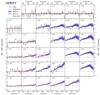 |
Fig. A.4. Same as in Fig. B.1 but here for a verification data vector (black points with errors bars), this means fδ, mn ≡ 1 by construction, with added random noise based on the error covariance matrix for KiDS-1000. |
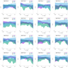 |
Fig. A.5. Illustration of possible variations in fδ(k, z) reconstructions (68% CIs about the median) using τ = 5.0 and Nk = 20 on noisy data vectors from the ray-traced KiDS-1000 mock-data which has fδ ≈ 1 (Sect. 5.5). There is a tendency for fδ > 1 in Z3 = [0.6, 2] (cyan), and a tendency for fδ < 1 in Z2 = [0.3, 0.6] (green) due to skewed PDFs and correlated errors. The magenta region shows the constraints for Z1 = [0, 0.3] which are the tightest compared to Z2 and Z3. An average over many reconstructions is shown in the bottom panel of Fig. 6. |
Appendix B: Posterior predictive for KiDS-1000 data
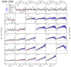 |
Fig. B.1. Posterior predictive of the Bayesian analysis using KiDS-1000 tomographic shear correlations and a relative power, fδ(k, z), averaged inside the three redshift bins Z1 = [0, 0.3], Z2 = [0.3, 0.6], and Z3 = [0.6, 2]. For each tomographic bin combination (ij), the panels with labels ‘z–ij’ show the posterior model constraints as light blue (95% CI) regions and dark blue (68% CI) regions about the median for either θ ξ−(ij)(θ) (lower left triangle) or θ ξ+(ij)(θ) (upper right triangle), both in units of |

All Tables
Parameters of the reference power spectrum, Pδfid(k, z), and the projection parameters (lensing kernel, IA) used to infer fδ(k, z) = Pδ(k, z)/Pδfid(k, z).
All Figures
|
Fig. 1. Probability density distribution functions, pz(i)(z), of KiDS-1000 source galaxies within the five tomographic redshift bins (from i = 1 to i = 5): (0.1, 0.3], (0.3, 0.5], (0.5, 0.7], (0.7, 0.9], and (0.9, 1.2]. These estimates are from Hildebrandt et al. (2021). |
| In the text | |
|
Fig. 2. Impact of the Tikhonov regularisation used to suppress oscillating solutions fδ(k, z). Shown are, for a noise-free mock data vector and the KiDS-1000 error covariance, the posterior constraints (68% credible regions) on fδ averaged over the redshift bin Z1 = [0, 0.3] (left), Z2 = [0.3, 0.6] (middle), and Z3 = [0.6, 2] (right) with and without regularisation (dark orange τ = 5.0 with median as dashed line or light orange τ = 0). To boost scale-dependence and evolution, fδ(k, z) is here defined relative to the power spectrum at fixed redshift, probing the relative structure growth since z = 1. The solid line is the median posterior fδ for 100× reduced measurement errors, providing a nearly noise-free reference (noise/100) that averages the growth over the redshift bin while still exhibiting artefacts near the edges. The dotted lines are the theoretical |
| In the text | |
|
Fig. 3. Test of data against a null model with identical |
| In the text | |
|
Fig. 4. Reconstructed matter power spectrum in KiDS-1000 for τ = 5.0 and Nk = 20 in three variants. The errors marginalise over uncertainties in the lensing kernel and IA. Shown are the posterior 68% CI about the median (lines). Left panel: Transfer function fδ(k, z) averaged over the entire redshift range Z1 = [0, 2] and relative to the reference, Pδfid(k, z), with parameters listed in Table 1. Middle panel: Same as the left panel, but for three independent transfer functions averaged separately within the ranges Z1 = [0, 0.3], Z2 = [0.3, 0.6], and Z3 = [0.6, 2]. Right panel: Dimensionless power spectrum, Δ2(k, z) = 4π k3Pδ(k, z) = 4π k3 fδ(k, z) Pδfid(k, z), interpolated to the centres of three redshift bins Z1, Z2, and Z3. |
| In the text | |
|
Fig. 5. Correlation matrix of fδ, mn errors for the KiDS-1000 analysis with three redshift bins, corresponding to the middle and right panels in Fig. 4. The three blocks on the diagonal from bottom left to top right are the correlation matrices for the z-bins Z1 = [0, 0.3], Z2 = [0.3, 0.6], Z3 = [0.6, 2], respectively; off-diagonal blocks show correlations between distinct z-bins; pixels within the 20 × 20 blocks are correlations between the k-bins, ascending from left to right inside a block. |
| In the text | |
|
Fig. 6. Verification test of the analysis code for fδ(k, z) using: an N-body simulated data vector, averaged over n = 1944 realisations of the KiDS-1000 data without IA; the code and data set-up for the KiDS-1000 analysis has Nk = 20 k-bins and three redshift bins Z1 = [0, 0.3], Z2 = [0.3, 0.6], and Z3 = [0.6, 2]. The reference power, Pδfid(k, z), is here identical to the cosmology of the simulation (Takahashi et al. 2017). The errors (68% CI) do not marginalise over a projection kernel uncertainty. Top panel: Simulated covariance of the average data, comprising n times the area of KiDS-1000. Deviations from the expected fδ(k, z) = 1 towards higher z and k ≳ 1 h Mpc−1 are related to the finite grid pixel size in the simulation (pixelation bias). The lines are additional reconstructions using noise-free data, based on Eq. (8) and halofit without pixelation bias. Bottom panel: Same as top panel, but with statistical errors as in a single KiDS-1000 survey. |
| In the text | |
|
Fig. 7. Percentage fraction in total marginal posterior error of fδ, mn due to uncertainties in the lensing kernel and IA parameter. Shown is the statistical error relative to the full marginal error (RMS variance of posterior) as a function of k in three redshift bins without marginalisation (solid lines), with marginalisation over errors in the source redshift distributions only (dashed lines), Ωm in the lensing kernel only (dash-dotted lines), and for the AIA error only (dotted lines). |
| In the text | |
|
Fig. 8. Power spectrum ratio ΔKiDS2(k, z)/ΔPlanck2(k, z) at z = 0.5. Shown in grey are the 68% and 95% CI from our analysis. The KiDS-1000 spectrum ΔKiDS2(k, z) uses the fδ, mn in Fig. 4 averaged within one broad redshift bin (left panel). The Planck model for ΔPlanck2(k, z) is the TT, TE, EE+lowE best fit of a standard ΛCDM (Planck Collaboration VI 2020) extrapolated to z = 0.5 with HMCode2020 by Mead et al. (2021). The lines are model transfer functions to ΔPlanck2(k, z) invoking flavours of extreme baryonic feedback (HMCode2020: log10(TAGN/K) = 8.8, Abaryon = 3.13, ηbaryon = 0.603; BCM by Schneider & Teyssier 2015: log10(Mc/h−1 M⊙) = 15.0792, ηb = 0.5, ks = 55.0), neutrino suppression for cumulative neutrino masses ∑νmν (BCM), or a mixture of CDM and WDM (Kamada et al. 2016, mwdm: WDM particle mass, fwdm: WDM mass fraction). |
| In the text | |
|
Fig. 9. KiDS-1000 results for fδ, mn, as in the middle panel of Fig. 4, in relation to alternative hypotheses using the reference cosmology Pδfid(k, z) and best-fitting bias parameters to match the KiDS-1000 data vector, ξ±(ij)(θ). The filled squares assume shear m-bias factors {mi}={+1.00, +0.48, −0.023, −0.028, +0.035}, the filled circles assume photo-z biases {δzi}={−0.075, −0.079, +0.009, +0.018, −0.052}, and the open diamonds employ the eNLA model with {AIA′,zpiv, η}={0.3, 0.19, 1.5}. The crosses assume a hybrid model of eNLA and a smaller z-bias: {AIA′,zpiv, η}={0.45, 0.25, 2.3} and {δzi}={−0.017, −0.058, +0.027, +0.025, −0.043}. The data points indicate the posterior median (CIs are similar to those of the shaded regions); the filled data points use alternating k-bins to avoid overlap. |
| In the text | |
|
Fig. A.1. Diagnostic plots of the Hamiltonian MCMC sampler with KiDS-1000 data and our final analysis set-up for fixed projection parameters as in Table 1. Top panel: Example of fδ, mn variations along one random chain at the beginning of the burn-in, starting from the random initial point i = 0 (blue line). The orange line depicts the (negative log-) posterior probability −2lnP(πi|d). Bottom panel: Decrease in the correlation of fδ, mn and fδ, kl with δi iterations lag as estimated in ten randomly chosen, independent chains. The orange lines follows, one line per chain, the maximum absolute-value Pearson correlation coefficient |Rmn, kl|, while the blue lines follows the average |Rmn, kl| over all variable combinations (mn, kl). The sampling points quickly decorrelate after a few hundred iterations; the flattening after lag δi ∼ 100 is due to the statistical error in the estimated |R| for chains of finite length nmcmc = 5 × 10⁴. |
| In the text | |
|
Fig. A.2. Reconstructed relative power spectrum, fδ(k, z), in redshift range 0 ≤ z < 2 using a verification data vector mimicking KiDS-1000 data (noise added, not marginalising IA or lensing kernel errors). The true relative power has fδ ≡ 1 for all scales and redshift. The data vector is computed from an independent code, not based on the projection matrix X(ij)(θ; m, n). Shown is the posterior median within a 68% CI. The reconstructions use a Tikhonov parameter of τ = 5.0 and Nk = 20 k-bins. Left panel: The relative power is averaged over the entire redshift range Z1 = [0, 2]. Middle panel: For a relative power that is averaged independently for three redshift bins Z1 = [0, 0.3], Z2 = [0.3, 0.6], and Z3 = [0.6, 2]. Right panel: Dimensionless average power spectrum, Δ2(k, z) = 4π k3Pδfid(k, z) fδ(k, z), interpolated to the centres of the redshift bins Z1 to Z3. |
| In the text | |
|
Fig. A.3. Posterior PDF of fδ, mn at |
| In the text | |
|
Fig. A.4. Same as in Fig. B.1 but here for a verification data vector (black points with errors bars), this means fδ, mn ≡ 1 by construction, with added random noise based on the error covariance matrix for KiDS-1000. |
| In the text | |
|
Fig. A.5. Illustration of possible variations in fδ(k, z) reconstructions (68% CIs about the median) using τ = 5.0 and Nk = 20 on noisy data vectors from the ray-traced KiDS-1000 mock-data which has fδ ≈ 1 (Sect. 5.5). There is a tendency for fδ > 1 in Z3 = [0.6, 2] (cyan), and a tendency for fδ < 1 in Z2 = [0.3, 0.6] (green) due to skewed PDFs and correlated errors. The magenta region shows the constraints for Z1 = [0, 0.3] which are the tightest compared to Z2 and Z3. An average over many reconstructions is shown in the bottom panel of Fig. 6. |
| In the text | |
|
Fig. B.1. Posterior predictive of the Bayesian analysis using KiDS-1000 tomographic shear correlations and a relative power, fδ(k, z), averaged inside the three redshift bins Z1 = [0, 0.3], Z2 = [0.3, 0.6], and Z3 = [0.6, 2]. For each tomographic bin combination (ij), the panels with labels ‘z–ij’ show the posterior model constraints as light blue (95% CI) regions and dark blue (68% CI) regions about the median for either θ ξ−(ij)(θ) (lower left triangle) or θ ξ+(ij)(θ) (upper right triangle), both in units of |
| In the text | |
Current usage metrics show cumulative count of Article Views (full-text article views including HTML views, PDF and ePub downloads, according to the available data) and Abstracts Views on Vision4Press platform.
Data correspond to usage on the plateform after 2015. The current usage metrics is available 48-96 hours after online publication and is updated daily on week days.
Initial download of the metrics may take a while.